Seediscussions,stats,andauthorprofilesforthispublicationat:http://www.researchgate.net/publication/4239340

Causalinversionofasingle-linkflexible-linkmanipulatorviaoutputplanning

CONFERENCEPAPER·JANUARY2005

DOI:10.1109/ICMA.2005.1626576·Source:IEEEXplore

CITATIONS

3

3AUTHORS,INCLUDING:

M.Vakil

UniversityofSaskatchewan

27PUBLICATIONS64CITATIONS

SEEPROFILE

R.Fotouhi

UniversityofSaskatchewan

31PUBLICATIONS101CITATIONS

SEEPROFILE

Availablefrom:M.Vakil

Retrievedon:25August2015

Proceedings of the IEEE International Conference on Mechatronics & Automation Niagara Falls, Canada • July 2005

0-7803-9044-X/05/$20.00 © 2005 IEEE

Causal Inversion of a Single-Link Flexible-Link Manipulator via Output Planning

M Vakil, R. Fotouhi, P. N. Nikiforuk

Department of Mechanical Engineering University of Saskatchewan

Saskatoon, Saskatchewan, Canada, S7N 5A9 {mov955@mail., reza.fotouhi@, peter.nikiforuk@}usask.ca

Abstract - Recently, a method was introduced by Bensoman and Le Vey [1] for the stable inversion of a single-input single-output (SISO) non-minimum phase system through the employment of output planning. The use of a causal input via output planning permits the initial conditions to be freely selected. In the application of this method to a single-link flexible-link manipulator (SFLM), for any initial conditions a polynomial is sought for the end-effector’s trajectory that cancels the effects of the internal instability of the inverse system. A drawback of this method, however, is that allows for the development of only one polynomial for any initial conditions imposed on the input and output. An extension of this method is proposed in this paper which does not suffer from this drawback. This extension employs exponential functions to define the end-effector’s trajectory, which leads not to just one solution, but to a family of solutions. The results of some simulation studies that verify the proposed extension are included.

Index Terms – Output planning, flexible link manipulator

I. INTRODUCTION

Because of their potential application in a wide range of operation, flexible-link manipulators have been widely studied over a number of years. Many of these studies have been on the end-effector’s trajectory planning [1, 3, 4, 5]. One possibility for the end-effector’s trajectory tracking is adopting the regulation method introduced in [2]. The feasibility of applying this method to flexible-link manipulators is studied in [3]. Another alternative for the end-effector’s trajectory tracking is to create a feedforward control command by using the inversion of the system dynamic. Inversion of a minimum phase system, such as end-effector’s motion of rigid-link manipulators, is done very easily. Contrary to rigid-link manipulators the end-effector’s trajectory tracking of flexible-link manipulators has non-minimum phase characteristics. Thus, the causal stable inversion of the dynamic equation of flexible-link manipulators having a desired trajectory for the end-effector is not achievable. To force the end-effector of a SFLM to follow a specific path, the required bounded torque is obtained by the non-causal inversion of the equation of motion in the frequency domain [4]. Using Laplace transformation, Kwon and Book [5] solved the same problem of end-effector’s trajectory inversion for a SFLM. The methods introduced in [4, 5] find the proper initial conditions for the inverse system so that the result of the inverse system becomes bounded. Moreover, these inversion procedures are

applicable if the equations which represent the forward dynamic are hyperbolic. For a linear system, the hyperbolic characteristic of these equations equal to the non-existing purely imaginary zeros for the transfer function of the forward system. Recently, a method was introduced by Bensoman and Le Vey [1] that starts from any initial conditions for the inverse equation of a SFLM and searches for the proper desired output that leads to the stable inversion of a SFLM. The desired output, however, is a polynomial of a specific order. This method is applicable for the stable inversion of both hyperbolic and non-hyperbolic systems. In this paper the method used in [1] is extended to the case where the desired output is a combination of several exponential functions, rather than a polynomial function, which makes the inverse system stable. The number of the exponential functions used to construct the desired output is equal to the order of the polynomial used in [1]. Further, while the method in [1] results in just one polynomial function for the output, our proposed method produces a family of answers. Our method, therefore, achieves the same goals that are presented in [1] but with additional features. In our proposed method, and also the method presented in [1], the desired output is planned; the only constraints that are imposed are on initial and final values and the derivatives of the end-effector’s trajectory. In general, however, it is more desirable to give the desired end-effector’s trajectory rather than planning it. Due to the variety of choices available for the desired trajectory, the designer has wider choices to choose the trajectory closer to the required one.

II. MATHEMATICAL ASPECTS

For a flexible-link manipulator u is the input torque and y is the end-effector’s position. In the inverse system, which we are dealing with, y is the input, referred to as “desired output”, and u is the “calculated output”. For a single-input single-output (SISO), linear-time- invariant (LTI) system, the dynamic equation can be written as:

ByAu = (1) where

=

=p

ii

i aDA0

(2)

376

=

=h

ii

i bDB0

(3)

i

ii

dtdD

)(= (4)

)..2,1,0( piai = and )..2,1,0( hibi = are real constants.

Let dy be the desired output to be tracked. The

feedforward control torque, u, the “calculated output”, is obtained by solving the following differential equation:

dByAu = (5)

The solution u consists of the complementary solution of the following homogenous ODE (Eq.6) and particular solution

of dp ByAu = .

0=cAu (6)

Since the coefficients of the differential operator A are constant, the complementary solution is:

trp

iic

iecu=

=1

(7)

where ir are the roots of the characteristic equation of (6),

A(r) = 0. If Eq.1 represents a non-minimum phase dynamic

system, some ir will have positive real values that result in

unstable response of the system. The purely imaginary roots

ir will result in non-vanishing oscillatory responses.

Therefore, they will also be considered as unstable roots.

Adding the particular solution, pu , of Eq.1 to the

complementary solution, cu , the general solution, u , is:

cp uuu += (8)

The coefficients ic in Eq.7 are found from the initial

conditions imposed on u.

III. STABLE EXPONENTIAL OUTPUT PLANNING

In this section the stable inversion of Eq.1 via output planning will be explained. It will be shown, while satisfying the required initial and final conditions imposed on y and also initial conditions imposed on u, it is possible to plan the desired output so that cu do not have unstable parts (The

values of ic that correspond to unstable roots ir become

zeros). It is assumed that the desired output is a combination of exponential functions:

tmi

g

id

ieky=

=1

(9)

in which im are negative real constants. The value of

contribution of each exponential function ( ik ) in constructing

the desired output will be chosen such that: 1- The unstable response of the u is not excited (i.e., positive and purely imaginary roots of 0=cAu )

2- The initial conditions on u are satisfied 3- The initial and final conditions on dy are satisfied

For a single exponential function, for a desired output mtkey = (10)

the particular solution of u is:

mtpy zeu = (11)

where

=

== p

i

ii

h

i

ii

ma

mbkz

0

0 (12)

Remark 1: m in Eq.10 can be any negative number except the negative roots of the characteristic equations A(m)=0, B(m)=0 of (2) and (3) (i.e. 0)(,0)( ≠≠ mBmA ), in which case the

value of z will be zero or infinity. Since m is a given known negative real number, k is

calculated to satisfy the triple conditions imposed on ik as

given above. The number of k’s to be calculated must be equal to the number of constrained equations.

Consider that the following initial and final conditions are imposed on y:

1

1

2

2

1

1

0

1

1

2

2

1

1

0

)(....,)(,)(,)(

)(.....,)(,)(,)(

−−

−−

====

====

fnfn

ffffff

iqiq

iiiiii

ytyytyytyyty

ytyytyytyyty

(13)

where it and ft are the initial and final times, i

ii

dtydy = , with

q-1 and n-1 being the highest order of derivatives of y that have to be satisfied at it and ft , respectively. It is worth

mentioning that in the forward system, to have a unique solution for y , the number of initial conditions imposed on yhave to be equal to the order of the forward differential equation (i.e. q-1 = h).

In addition to the above conditions on y consider the following initial conditions that have to be satisfied on u

1

1

2

2

1

1

0 )(.....,)(,)(,)( −− ==== iwi

wiiiiii utuutuutuutu (14)

where it is the initial time, i

ii

dtudu = , with w-1 being the

highest order of derivative of u that has to be satisfied at it . It

is worth mentioning that in the inverse system, to have a unique solution for u, the number of initial conditions on uhave to be equal to the order of the inverse system’s differential equation (i.e. w-1 = p).

Having the desired initial and final conditions imposed on y and u and also the number of unstable roots of the characteristic equation of (2), A(r) = 0, the required number of exponential functions is calculated. If g is the required number of exponential functions, then g is (details are given at the appendix):

g = q + n + w +e – p (15) where e is the number of unstable roots of the characteristic equation of (2), A(r) = 0, w is the number of initial conditions on u, q is the number of initial conditions on y, n is the number of final conditions on y, and p is the number of unknown coefficients of cu .

Remark 2: The unstable roots of the characteristic equation of (2), A(r) = 0, may be pure imaginary roots or complex roots with positive real parts. While the non-causal integration is not applicable for purely imaginary roots, the method presented

377

here is applicable.

Remark 3: It is clear that the im in Eq. 9 is decided at the

beginning of the procedure. They can be any negative numbers except the negative roots of the characteristic equations A(m)=0 and B(m)=0 of (2) and (3). Therefore, the inversion method presented here via output planning results in a family of solutions rather than just one polynomial solution as given by [1].

Having calculated the number of exponential functions from Eq. 15, the unknowns (k in Eq.10, z in Eq.11 and c in Eq.7) are found by solving a set of simultaneous linear algebraic equations.

IV. SFLM STABLE INVERSION THROUGH OUTPUTPLANNING

In this section the stable inversion of a SFLM by output planning will be examined. The dynamic model from [1] is used for simulation. Due to finite wave propagation in elastic media there is a time delay between actuation and sensing if the actuator and sensor are non-collocated. In a linear model, this delay is represented by a zero at the right hand side of the S-plane. Because of the existence of such positive zeros the linear system is non-minimum phase. Usually for a flexible-link manipulator, the input is the torque at the base and the desired output is the end-effector’s position. Thus, the relation between the input (torque) and the output (end-effector’s position) has a non-minimum phase characteristic. The dynamics of the flexible-link manipulator is of infinite-dimension. Usually a truncated dynamic model based on the assumed mode shape method (AMM) [5], or finite element method (FEM) [6], is used to control the motion of a flexible-link manipulator. Use of the AMM for trajectory tracking of a flexible-link manipulator at the joint space is studied in [7]. In this paper the dynamic modeling based on the AMM is also used.

The lateral displacement of a point at a distance x from the base as in Fig. 1, is obtained as the sum of rigid body rotation (θ ) and the small deflection (ζ ):

ζθδ += x (16)

It is assumed that ζ (lateral displacement of point x in

flexible-link manipulator measured from rotated rigid-link manipulator) is small and given by:

i

n

ii x λϕζ

=

=1

)( (17)

where iϕ is any kinematically admissible function (usually iϕis chosen as the mode shapes of the free vibration of the

clamped-free beam) and iλ are scalar weight functions.

The kinetic (Ke) and potential (Pe) energies of the link in the horizontal plane are:

dxdxdEIPe

L

2

2

2

2

1= ζ (18)

KtpKhdxdtdKe

L

++= )2

1(

2δρ (19)

where

EI : Link’s rigidity

ρ : Mass per unit length

Kh : Hob’s kinetic energy

Ktp : Tip-mass’s kinetic energy

Using the Lagrangian approach, the dynamic equation of the motion for the SFLM is obtained as:

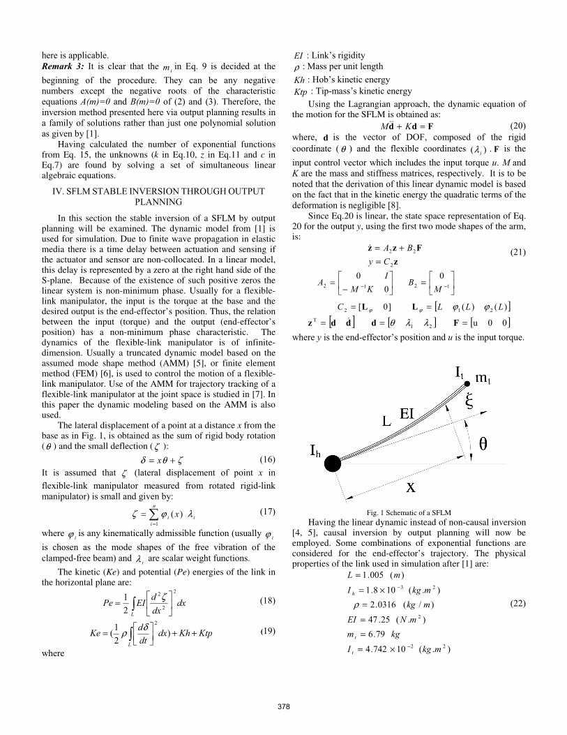
Fdd =+ KM (20)

where, d is the vector of DOF, composed of the rigid

coordinate ( θ ) and the flexible coordinates )( iλ . F is the

input control vector which includes the input torque u. M and K are the mass and stiffness matrices, respectively. It is to be noted that the derivation of this linear dynamic model is based on the fact that in the kinetic energy the quadratic terms of the deformation is negligible [8].

Since Eq.20 is linear, the state space representation of Eq. 20 for the output y, using the first two mode shapes of the arm, is:

zFzz

2

22

CyBA

=+= (21)

[ ])()(]0[

0

0

0

212

1212

LLLC

MB

KMI

A

ϕϕϕϕ ==

=−

= −−

LL

[ ] [ ] [ ]00u21

T === Fdddz λλθwhere y is the end-effector’s position and u is the input torque.

Fig. 1 Schematic of a SFLM Having the linear dynamic instead of non-causal inversion

[4, 5], causal inversion by output planning will now be employed. Some combinations of exponential functions are considered for the end-effector’s trajectory. The physical properties of the link used in simulation after [1] are:

)(005.1 mL = ).(108.1 23 mkgI h

−×=)/(0316.2 mkg=ρ (22)

).(25.47 2mNEI = kgm t 79.6= ).(10742.4 22 mkgI t

−×=

378

The first and second natural frequencies of such clamped-free beam are Hz03.61 =f and Hz07.162 =f as noted in

[1]. The transfer function which relates the desired end-effector’s position “y” and the input torque “u” is [1]:

).s.(ss

.s.s.uy

8082517935622431901542

63633319562736984295

++

++−= (23)

This transfer function is obtained assuming two mode shapes and using physical parameters given in (22). The transfer function’s zeros are:

±=±=

izz

5.56

4.59

4,3

2,1 (24)

Since there was no damping consideration in the single-link flexible-link manipulator presented in [1], there exist purely imaginary zeros. While the existence of pure imaginary zeros is a barrier in application of the non-causal integration method introduced in [4, 5], our method can handle the existence of pure imaginary zeros. To determine the number of exponential functions that must be used for output planning consider that the following initial conditions are imposed on yand u and their derivatives and also the following final conditions are imposed on y and its derivatives:

0)0()0()0()0()0()0( 54321 ====== yyyyyy (25)

0)0()0()0()0( 321 ==== uuuu (26)

and

0)10()10(

57.1)10(

21 ===

yyy

(27)

To find the output y in the time domain from the transfer function given in Eq.23 zero initial conditions on y and its first five derivatives (Eq.25) and zero initial conditions on u and its first three derivatives (Eq.26) are assumed. It is also assumed that the duration of motion is 10 seconds ( )10=ft . To find the

number of stable exponential functions the method described in Section III with the details in Appendix is used. The number of equations that must be satisfied because of the initial and final conditions imposed on y is q + n = 6 + 3 = 9. The number of equations that must be satisfied because of the initial conditions imposed on u is w = 4. The number of unknowns in the complementary answer of u is p = 4, and the number of unstable roots of the characteristic equation of A(r)=0 is e = 3 (2 imaginary, 1 positive roots).

Using Eq.15, the number of the exponential functions that must be used for output planning is:

g = 6 + 3 + 4 + 3 - 4 = 12 So:

=

=12

1i

tmi

ieky (28)

Three different sets of im were used for the simulation

studies. The im were not chosen totally arbitrary. They were

chosen using values corresponding to a single exponential function, ftmkey = ; assuming that we wish the function to be

reduced to one tenth of its initial value at the end of maneuver; i.e., ky

ft1.0

10=

=, this produces )1(.1. Lnm = or 23.−=m ;

this value was chosen as the starting point for choosing other

im values.

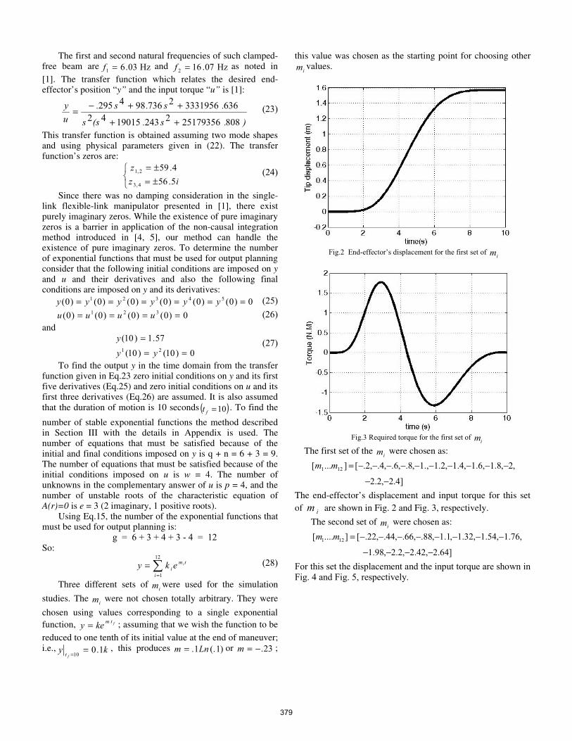
Fig.2 End-effector’s displacement for the first set of im

Fig.3 Required torque for the first set of imThe first set of the im were chosen as:

]4.2,2.2

,2,8.1,6.1,4.1,2.1.,1,8.,6.,4.,2.[]...[ 121

−−

−−−−−−−−−−=mm

The end-effector’s displacement and input torque for this set of im are shown in Fig. 2 and Fig. 3, respectively.

The second set of im were chosen as:

]64.2,42.2,2.2,98.1

,76.1,54.1,32.1,1.1,88.,66.,44.,22.[]....[ 121

−−−−

−−−−−−−−=mm

For this set the displacement and the input torque are shown in Fig. 4 and Fig. 5, respectively.

379

Fig. 4 End-effector’s displacement for the second set of

im

Fig. 5 Required torque for the second set of im

Fig. 6 End-effector’s displacement for the third set of im

Fig. 7 Required torque for the third set of im

Fig. 8 End-effector’s displacement for the fourth set of im

Fig.9 Required torque for the fourth set of imThe third set of im were chosen as:

]88.2,64.2,4.2,16.2

,92.1,68.1,44.1,2.1,96.,72.,48.,24.[]....[ 121

−−−−

−−−−−−−−=mm

380

For this set the displacement and input torque are shown in Fig. 6 and Fig. 7, respectively. A comparison of these three sets indicated the dependence of the required torque and the end-effector’s displacement on the values of the im . Since no

overshoot in the tip-displacement is desired, the first set of imis considered to be the best. Decreasing the values of the imcauses overshoots in end-effector’s response. Also some values of im resulted in a response that did not satisfy the

required initial condition. This clearly shows that not all possible combinations of im are satisfactory. For example for

a fourth set of im as:

]2.1,1.1,1,9.,8.,7.,6.,5.,4.,3.,2.,1.[]......[ 121 −−−−−−−−−−−−=mmThe end-effector’s displacement and required torque are shown in Fig. 8 and Fig. 9. It can be seen that this set violate initial conditions on u and y. To find the contribution of each exponential function a set of linear algebraic equations must be solved. If these equations are not linearly independent then determinant of the coefficient matrix becomes zero, which results in an unacceptable response (the fourth set is an example).

V. CONCLUSION

Recently in [1] the causal inversion of SISO LTI systems via output planning was studied. The planned desired output was a polynomial. In the method presented in this paper the planned desired output is a combination of exponential functions. Unlike the method presented in [1], which creates only one polynomial function for the given initial and final conditions, the method presented here leads to a family of exponential functions. Thus the planned desired output is chosen from a family of solutions.

The method presented here and also that of [1] create a desired output that only satisfies given initial and final conditions. Generally, it is desirable to give the desired output rather than planning it. Due to the variety, which is given by our method, in choosing the planned output, the designer is free to select the desired output.

Comparing the method presented here and that in [1], it can be shown that the planned output can be a combination of the polynomial function presented in [1] and the exponential functions presented here.

APPENDIX

CALCULATING THE NUMBER OF EXPONENTIALFUNCTIONS USED IN PLANNING DESIRED OUTPUT

Consider that the number of unstable roots (positive plus purely imaginary) of the characteristic equation of A(r)=0 is equal to e (e.g e = 3 in IV). Let the required number of exponential functions be g. The number of initial and final conditions imposed on y, (Eq.13) is q + n (e.g. q+n=6+3=9 in IV). The number of initial conditions imposed on u, (Eq.14) is w (e.g. w=4 in IV). According to Eq.12 there is a linear relation between the coefficients of pyu in Eq.11 and the

corresponding y in Eq.10. Therefore, if the required number of exponential function is g, there are g relations between all the

z and k. The number of unknowns for the complementary solution in Eq.6 is p (if the order of A in IV is 4, there is 4 icin Eq.7, thus p is equal to 4). The number of unknowns based on the number of exponential functions used for planning the desired output is 2g. The contribution of each exponential function, ik in Eq. 9 is unknown. Also z, in Eq.11 for each

pyu is unknown. Thus there are 2g unknowns. The total

number of unknowns is p + 2g - e (e.g. 4 + 2g - 3 in IV). The total number of available equations is q + n + w + g (e.g. 6 + 3 + 4 + g in IV). Remark 4: To eliminate the unstable part of cu (positive or

purely imaginary roots of A) the coefficient ic related to the

unstable parts has to be zero. If the number of these unstable poles is e, e out of p of the coefficients of ic must be zero.

Then the number of unknowns is p + 2g - e (e.g. 4 + 2g – 3 in IV). Thus g, the number of exponential functions that must be used in planning the desired output is obtained as:

pewnqg −+++= (A1)

(e.g, g = 6 + 3 + 4 + 3 - 4 = 12 in IV).

The desired output is then of the form =

=g

i

tmid

ieky1

REFERENCES

[1] M. Benosman and G. Le Vey, Stable inversion of SISO nonminimum phase system through output planning : An experimental application to the one-link flexible manipulator, IEEE Transactions on Control System Technology, Vol. 3, No. 4, July 2003, pp. 588-597

[2] A. Isidori and C. Byrnes, Output regulation of nonlinear system, IEEE Transactions on Automation and Control, Vol. 35, Feb 1990, pp. 131-140.

[3] A. De Luca , L. Lanari, and G. Ulivi, End-effector trajectory tracking in flexible arms. Comparison of approaches based on regulation theory, Lecture Notes in Control and Information Sciences, Vol. 162, 1991, pp. 190-206

[4] E. Bayo, A finite-element approach to control the end-point motion of a single link flexible robot, International Journal of Robotics Systems, Vol. 4, No. 1, 1989, pp. 63-75.

[5] D. S. Kwon and W. J. Book, Time-domain inverse dynamic tracking control of a single-link flexible manipulator, Journal of Dynamic Systems, Measurement and Control, Transactions of the ASME, Vol. 116, No. 2, June 1994, p.193-200.

[6] Y. A. Khulief, Vibration suppression in rotating beams using active modal control, Journal of Sound and Vibration, Vol. 242, No. 4, May 2001, pp. 681-699.

[7] M. Vakil, R. Fotouhi and P. N. Nikiforuk, Trajectory tracking of a single-link flexible link manipulator, the 20th Canadian Congress on Applied Mechanics (CANCAM), Montreal, Canada, May 30-June 2, 2005.

[8] A. De Luca and B. Siciliano, Closed-form dynamic model of planar multilink lightweight robots, IEEE Transactions on Systems, Man and Cybernetics, Vol. 21, No. 4, 1991, pp. 826-839.

[9] D. Wang and M. Vidyasagar, Control of class of manipulators with a single flexible link-Part I: feedback linearization, Journal of Dynamic Systems, Measurement and Control, Vol. 113, Dec 1991, pp. 655-661.

381