Improving Color Reproduction Accuracy on Cameras

Hakki Can Karaimer Michael S. Brown

York University, Toronto

{karaimer, mbrown}@eecs.yorku.ca

Abstract

One of the key operations performed on a digital cam-

era is to map the sensor-specific color space to a standard

perceptual color space. This procedure involves the appli-

cation of a white-balance correction followed by a color

space transform. The current approach for this colorimet-

ric mapping is based on an interpolation of pre-calibrated

color space transforms computed for two fixed illumina-

tions (i.e., two white-balance settings). Images captured

under different illuminations are subject to less color ac-

curacy due to the use of this interpolation process. In this

paper, we discuss the limitations of the current colorimet-

ric mapping approach and propose two methods that are

able to improve color accuracy. We evaluate our approach

on seven different cameras and show improvements of up to

30% (DSLR cameras) and 59% (mobile phone cameras) in

terms of color reproduction error.

1. Introduction

Digital cameras have a number of processing steps that

convert the camera’s raw RGB responses to standard RGB

outputs. One of the most critical steps in this processing

chain is the mapping from the sensor-specific color space to

a standard perceptual color space based on CIE XYZ. This

conversion involves two steps: (1) a white-balance correc-

tion that attempts to remove the effects of scene illumina-

tion and (2) a color space transform (CST) that maps the

white-balanced raw color values to a perceptual color space.

These combined steps allow the camera act as a color repro-

duction, or colorimetric, device.

The colorimetric mapping procedure currently used on

cameras involves pre-computing two CSTs that correspond

to two fixed illuminations. The calibration needed to com-

pute these CSTs is performed in the factory and the trans-

form parameters are part of the camera’s firmware. The

illuminations that correspond to these calibrated CSTs are

selected to be “far apart” in terms of correlated color tem-

perature so that they represent sufficiently different illumi-

nations. When an image is captured that is not one of the

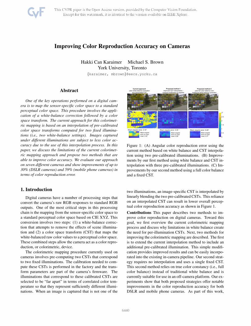
Mean angular error: 3.10° Mean angular error: 0.30 ° Mean angular error: 0.29°

Proposed method 2

uses full color-balance over

traditional white-balance correction

Current approach

uses white-balance correction

and interpolated CST

Mean angular

error on color

chart: 0.37°

Mean angular

error on color

chart: 0.58°

Mean angular

error on color

chart: 2.52°

Proposed method 1

improved CST interpolation -

minimal modification to pipeline

A B C°

Figure 1: (A) Angular color reproduction error using the

current method based on white balance and CST interpola-

tion using two pre-calibrated illuminations. (B) Improve-

ments by our first method using white balance and CST in-

terpolation with three pre-calibrated illuminations. (C) Im-

provements by our second method using a full color balance

and a fixed CST.

two illuminations, an image-specific CST is interpolated by

linearly blending the two pre-calibrated CSTs. This reliance

on an interpolated CST can result in lower overall percep-

tual color reproduction accuracy as shown in Figure 1.

Contributions This paper describes two methods to im-

prove color reproduction on digital cameras. Toward this

goal, we first overview the current colorimetric mapping

process and discuss why limitations in white balance create

the need for per-illumination CSTs. Next, two methods for

improving the colorimetric mapping are described. The first

is to extend the current interpolation method to include an

additional pre-calibrated illumination. This simple modifi-

cation provides improved results and can be easily incorpo-

rated into the existing in-camera pipeline. Our second strat-

egy requires no interpolation and uses a single fixed CST.

This second method relies on true color constancy (i.e., full

color balance) instead of traditional white balance and is

currently suitable for use in an off-camera platform. Our ex-

periments show that both proposed strategies offer notable

improvements in the color reproduction accuracy for both

DSLR and mobile phone cameras. As part of this work,

6440

White-balance

& color space

transformation

(CST)

White-balance

& color space

transformation

(CST)

Pre-processing

+ demosaicing

Sensor's raw

image

Photo-finishing

(tone mapping,

color

manipulation)

Final output

space color

conversion

(sRGB/YUV)

Stage 1: Colorimetric mapping Stage 2: Photo-finishing and output

Figure 2: A diagram of a typical in-camera imaging

pipeline. Work in this paper targets the colorimetric map-

ping in the first stage in this pipeline that converts the

camera-specific color space to a perceptual color space. The

procedure targeted by our work is highlighted in red and

represents an intermediate step in the overall pipeline.

we have also created a dataset of 700 carefully calibrated

colorimetric images for research in this area.

2. Motivation and related work

Motivation Before discussing related work, it is important

to understand the motivation of our work and its context

with respect to the in-camera pipeline. Figure 2 shows a

standard diagram of the processing pipeline [33, 28]. At a

high level, the overall pipeline can be categorized into two

stages: (1) a colorimetric conversion and (2) photo-finishing

manipulation. The first stage converts sensor RGB values

from their camera-specific color space to a perceptual color

space. The second stage involves a number of operations,

such as tone and color manipulation, that modify the im-

age’s appearance for aesthetic purposes.

Radiometric calibration methods (e.g., [8, 13, 14, 29, 40,

31]) target the reversal of the second stage to undo nonlinear

processing for tasks such as photometric stereo and high-

dynamic range imaging. Research on color reproduction

applied on the camera–that is, the first stage in the pipeline–

has seen significantly less attention. This is in part due to

the lack of access to the camera hardware, since this first

stage is applied onboard the camera. This restrictive access

was addressed recently by Karaimer and Brown [28], who

introduced a software-based camera emulator that works for

a wide range of cameras. This software platform allows the

pipeline to be stopped at intermediate steps and the interme-

diary pixel values to be accessed or modified. This platform

has enabled the work performed in this paper, allowing the

analysis of our proposed methods as well as the creation of

an image dataset to evaluate the results.

In the following, we discuss two areas related to camera

color reproduction: white balance and color calibration.

White balance and color constancy White balance (WB)

is motivated by a more complex procedure, color constancy,

that aims to make imaged colors invariant to a scene’s il-

lumination. Computational color constancy is performed

on cameras in order to mimic the human visual system’s

ability to perceive objects as the same color under differ-

ent illuminations [30]. Computational color constancy is a

two-step procedure: (1) estimate the scene illumination in

the camera’s sensor color space; (2) apply a transform to re-

move the illumination’s color cast. Most color constancy re-

search focuses only on the first step of illumination estima-

tion. There is a wide range of approaches for illumination

estimation, including statistical methods (e.g., [37, 21, 1]),

gamut-based methods (e.g., [23, 15, 24]), and machine-

learning methods (e.g., [2, 3, 11, 7]), including a num-

ber of recent approaches using convolutional neural net-

works (e.g., [27, 6, 35, 32]).

Once the illumination has been estimated, most prior

work uses a simple 3× 3 diagonal correction matrix that

can be computed directly from the estimated illumination

parameters. For most illuminations, this diagonal matrix

guarantees only that neutral, or achromatic, scene materi-

als (i.e., gray and white objects) are corrected [10]. As a

result, this type of correction is referred to as “white bal-

ance” instead of color balance. Because WB corrects only

neutral colors, the CST that is applied after WB needs to

change, depending on the WB applied, and thus the CST

is illumination-specific. This will be discussed in further

detail in Section 3.

There have been several works that address the short-

coming of the diagonal 3×3 WB correction. Work by Fin-

layson et al. [17, 18] proposed the use of a spectral sharp-

ening transform in the form of a 3×3 full matrix that was

applied to the camera-specific color space. The transformed

color space allowed the subsequent 3×3 diagonal WB cor-

rection to perform better. To establish the sharpening ma-

trix, it was necessary to image known spectral materials un-

der different illuminations. Chong et al. [12] later extended

this idea to directly solve for the sharpening matrix by using

the spectral sensitivities of the sensor. When the estimated

sharpening matrix is combined with the diagonal matrix,

these methods are effectively performing a full color bal-

ance. The drawback of these methods, however, is the need

to have knowledge of the spectral sensitivities of the under-

lying sensor or imaged materials.

Recent work by Cheng et al. [10] proposed a method to

compute a full color-balance correction matrix without the

need of any spectral information of the camera or scene.

Their work found that when scenes were imaged under spe-

cific types of broadband illumination (e.g., sunlight), the di-

agonal WB correction was sufficient to achieve full color

balance. They proposed a method that allowed images un-

der other illuminations to derive their full color correction

using colors observed under broadband spectrum. This ap-

proach serves as the starting point for our second proposed

method based on color balance instead of white balance.

Color calibration After white balance, a color space trans-

form is applied to map the white-balanced raw image to

a perceptual color space. Most previous work targeting

color calibration finds a mapping directly between a cam-

6441

Ground-truth

ColorChecker reflectanceInput illuminantCamera sensitivity

��CRCGCB� � � ⋱ �� r r r r

���� � �

����

���� ∙ ����� Mean reproduction

error: 2.31°�� ∙ ����

�� ∙ ���� �� ∙ ����

�� ∙ ���� Mean reproduction

error: 0.72°

Mean reproduction

error: 1.43°Mean reproduction

error: 0.53°

400 700 400 700 400 700

A B

°

wavelength wavelength wavelength

pow

er

pow

er

pow

er

0

1

0

1

0

1

Figure 3: This figure is modeled after Cheng et al. [11]. (A) Image formation in the camera color space for two different

illumination sources. (B) Result of a conventional diagonal WB (WD) and full color correction (WF ) applied to the input

images. Errors are computed as angular reproduction error (see Section 5.2). WB introduces notable errors for non-neutral

colors. In addition, errors affect different scene materials depending on the illumination. Full color balance introduces fewer

reproduction errors for all materials.

era’s raw-RGB values and a perceptual color space. Such

color calibration is generally achieved by imaging a color

rendition chart composed of color patches with known CIE

XYZ values. Notable methods include Funt and Bastani [4]

and Finlayson et al. [16, 19], who proposed a color calibra-

tion technique that eliminated the dependence on the scene

intensities to handle cases where the color pattern was not

uniformly illuminated. Hong et al. [26] introduced a color

space transform based on higher-order polynomial terms

that provided better results than 3×3 transforms. Finlayson

et al. [20] recently proposed an elegant improvement on the

polynomial color correction by using a fractional (or root)

polynomial that makes this high-order mapping invariant to

camera exposure. Bianco et al.’s [5] is one of the few works

that considered the white-balance process by weighting the

color space transform estimation based on the probability

distribution of the illumination estimation algorithm.

While the above methods are related to our overall goal

of color reproduction, these methods rely on a color ren-

dition chart imaged under the scene’s illumination to per-

form the colorimetric mapping. As a result, they compute

a direct mapping between the sensor’s RGB values and a

target perceptual color space without the need for illumina-

tion correction, or, in the case of [5], require knowledge of

the error distributions of the white-balance algorithm. Our

work restricts itself to the current pipeline’s two-step proce-

dure involving a camera color space illumination correction

followed by a color space transform.

3. Existing camera colorimetric mapping

In this section, we describe the current colorimetric map-

ping process applied on cameras. We begin by first pro-

viding preliminaries of the goal of the colorimetric map-

ping procedure and the limitations arising from white bal-

ance. This is followed by a description of the current

interpolation-based method used on cameras.

3.1. Preliminaries

Goal of the colorimetric mapping Following the nota-

tion of Cheng et al. [10], we model image formation using

matrix notation. Specifically, let Ccam represent a cam-

era’s spectral sensitivity as a 3×N matrix, where N is the

number of spectral samples in the visible range ( 400nm to

700nm). The rows of the matrix Ccam = [cR; cG; cB]T

correspond to the spectral sensitivities of the camera’s R,

G, and B channels.

Since our work is focused on color manipulation, we can

ignore the spatial location of the materials in the scene. As

a result, we represent the scene’s materials as a matrix R,

where each matrix column, ri, is a 1×N vector represent-

ing the spectral reflectance of a material. Using this nota-

tion, the camera’s sensor responses to the scene materials,

Φlcam

, for a specific illumination, l, can be modeled as:

Φlcam

= Ccam diag(l)R = Ccam LR, (1)

where l is a 1×N vector representing the spectral illumi-

nation and the diag(·) operator creates a N ×N diagonal

matrix from a vector (see Figure 3).

The goal of the colorimetric mapping of a camera is to

have all the colors in the scene transformed to a perceptual

color space. This target perceptual color space can be ex-

pressed as:

Φxyz = Cxyz R, (2)

where Cxyz is defined similar to Ccam but uses the percep-

tual CIE 1931 XYZ matching functions [25]. In addition,

the effects of the illumination matrix L are ignored by as-

suming the scene is captured under ideal white light–that is,

all entries of l are equal to 1.

The colorimetric mapping problem therefore is to map

the camera’s Φlcam

under a particular illumination l, to

the target perceptual color space with the illumination

corrected–that is, Φxyz .

Deficiencies in white balance As previously discussed, the

colorimetric mapping on cameras is performed in two steps.

6442

��

Pre-calibration Interpolation processCA

#

#

#

#

#

#

# # #

# # #

# # #

# # #

# # #

# # #

B Weighting functions

1

02500°K 6500°K

weig

ht

Correlated color temperature

g

(1-g)

����

����

6500°K

2500°K

���

���Illumination 2 (CCT 6500°K)

Illumination 1 (CCT 2500°K)

New input

#

#

#

����# # #

# # #

# # #

���(4300°K)

� = CCT��−1 − CCT��−1CCT��−1 − CCT��−1

4300∘K�� 2500∘K�16500∘K�2

��� = ���� + (1− �)���

������

CIE XYZ target

CIE XYZ target

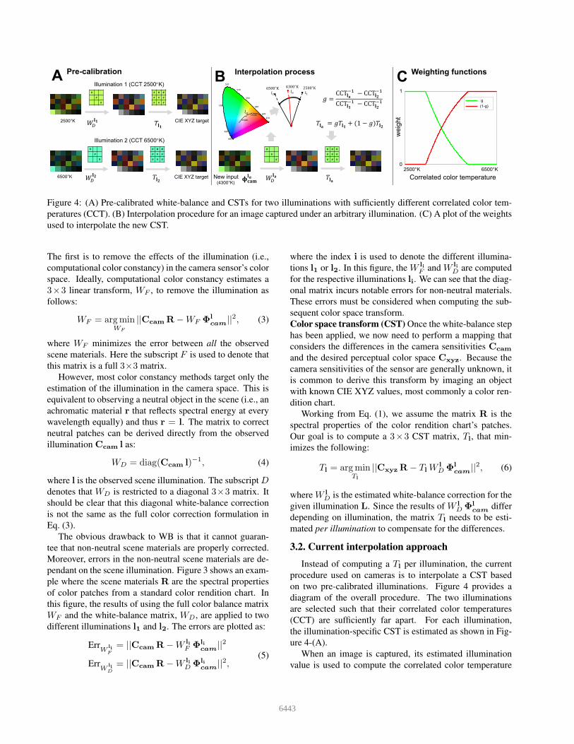
Figure 4: (A) Pre-calibrated white-balance and CSTs for two illuminations with sufficiently different correlated color tem-

peratures (CCT). (B) Interpolation procedure for an image captured under an arbitrary illumination. (C) A plot of the weights

used to interpolate the new CST.

The first is to remove the effects of the illumination (i.e.,

computational color constancy) in the camera sensor’s color

space. Ideally, computational color constancy estimates a

3×3 linear transform, WF , to remove the illumination as

follows:

WF = argminWF

||Ccam R−WF Φlcam

||2, (3)

where WF minimizes the error between all the observed

scene materials. Here the subscript F is used to denote that

this matrix is a full 3×3 matrix.

However, most color constancy methods target only the

estimation of the illumination in the camera space. This is

equivalent to observing a neutral object in the scene (i.e., an

achromatic material r that reflects spectral energy at every

wavelength equally) and thus r = l. The matrix to correct

neutral patches can be derived directly from the observed

illumination Ccam l as:

WD = diag(Ccam l)−1, (4)

where l is the observed scene illumination. The subscript D

denotes that WD is restricted to a diagonal 3×3 matrix. It

should be clear that this diagonal white-balance correction

is not the same as the full color correction formulation in

Eq. (3).

The obvious drawback to WB is that it cannot guaran-

tee that non-neutral scene materials are properly corrected.

Moreover, errors in the non-neutral scene materials are de-

pendant on the scene illumination. Figure 3 shows an exam-

ple where the scene materials R are the spectral properties

of color patches from a standard color rendition chart. In

this figure, the results of using the full color balance matrix

WF and the white-balance matrix, WD, are applied to two

different illuminations l1 and l2. The errors are plotted as:

ErrW

li

F

= ||Ccam R−WliF Φ

licam

||2

ErrW

li

D

= ||Ccam R−WliD Φ

licam

||2,(5)

where the index i is used to denote the different illumina-

tions l1 or l2. In this figure, the WliF and W

liD are computed

for the respective illuminations li. We can see that the diag-

onal matrix incurs notable errors for non-neutral materials.

These errors must be considered when computing the sub-

sequent color space transform.

Color space transform (CST) Once the white-balance step

has been applied, we now need to perform a mapping that

considers the differences in the camera sensitivities Ccam

and the desired perceptual color space Cxyz. Because the

camera sensitivities of the sensor are generally unknown, it

is common to derive this transform by imaging an object

with known CIE XYZ values, most commonly a color ren-

dition chart.

Working from Eq. (1), we assume the matrix R is the

spectral properties of the color rendition chart’s patches.

Our goal is to compute a 3×3 CST matrix, Tl, that min-

imizes the following:

Tl = argminTl

||Cxyz R− Tl WlD Φ

lcam

||2, (6)

where W lD is the estimated white-balance correction for the

given illumination L. Since the results of W lD Φ

lcam

differ

depending on illumination, the matrix Tl needs to be esti-

mated per illumination to compensate for the differences.

3.2. Current interpolation approach

Instead of computing a Tl per illumination, the current

procedure used on cameras is to interpolate a CST based

on two pre-calibrated illuminations. Figure 4 provides a

diagram of the overall procedure. The two illuminations

are selected such that their correlated color temperatures

(CCT) are sufficiently far apart. For each illumination,

the illumination-specific CST is estimated as shown in Fig-

ure 4-(A).

When an image is captured, its estimated illumination

value is used to compute the correlated color temperature

6443

#

#

#

#

#

#

# # #

# # #

# # #

# # #

# # #

# # #

��������

6500°K

5000°K

������

Illumination 3 (CCT 6500°K)

Illumination 2 (CCT 5000°K)

New input

#

#

#

����

��� = ���� + (1− �)���# # #

# # #

# # #

���(3000°K)

� = CCT��−1 − CCT��−1CCT��−1 − CCT��−1

5000∘K�3 2500∘K�16500∘K�2#

#

#

# # #

# # #

# # #����2500°K ���Illumination 1 (CCT 2500°K)

3000∘K����

������

1

02500°K 6500°K

weig

ht

Correlated color temperature

g

(1-g)

5000°K

CIE XYZ target

CIE XYZ target

CIE XYZ target

Calibration Interpolation processCA B Weighting functions

Figure 5: Our first method to improve the colorimetric mapping in the in-camera processing pipeline. (A) An additional

illumination is calibrated and added to the interpolation process. (B) Shows the overall procedure to compute the weights to

interpolate the CST. (C) Shows the weighting function for different estimated CCTs.

of the illumination [38, 34]. Based on the correlated color

temperature, the two pre-computed CSTs are interpolated

(see Figure 4-(B)) to obtain the final CST to be applied as

follows:

Tl = g Tl1 + (1− g) Tl2 , (7)

where

g =CCT−1

l − CCT−1

l2

CCT−1

l1− CCT−1

l2

. (8)

The factory pre-calibrated CCTs for l1 and l2 for most cam-

eras are selected to be 2500◦K and 6500◦K. The interpola-

tion weights of g and 1−g are shown in Figure 4-(C), where

the horizontal axis is the CCT of the image’s estimated illu-

mination.

As shown in Figure 1, this interpolation procedure based

on two fixed illuminations does not always provide good

results. In the following sections, we describe two methods

to improve the colorimetric mapping process.

4. Proposed improvements

We introduce two methods to improve the colorimetric

mapping procedure. The first approach is a simple exten-

sion of the interpolation method to include an additional

calibrated illumination in the interpolation process. The

second method relies on a full color correction matrix dis-

cussed in Section 3.1 and uses a fixed CST matrix for all

input images.

Method 1: Extending interpolation The most obvious

way to improve the current colorimetric mapping procedure

is to incorporate additional calibrated illuminations into the

interpolation process. Ideally we would like many illumi-

nations to be represented as control points in this process;

however, this is likely unrealistic in a factory pre-calibration

setting. As a result, we consider the case of adding only a

single additional interpolation control point with a CCT at

approximately 5000◦K. Figure 5-(A) shows a diagram of

our approach.

When a new image is obtained, we estimate the scene

illumination and then select which pair of pre-calibrated

Tl based on the estimated illumination’s CCT. The blend-

ing weights g and 1 − g are adjusted accordingly between

the pair of T selected using Eq. (8). The final CST, Tl,

is computed using Eq. (7). An example of this approach

is shown in Figure 5-(B). The weighting factors for g are

shown in Figure 5-(C). This simple inclusion of a single ad-

ditional pre-calibrated illumination in the interpolation pro-

cess gives surprisingly good results and can be readily in-

corporated into an existing in-camera pipeline.

Method 2: Using full color balance As discussed in Sec-

tion 2, our second method leverages the full color-balance

approach proposed by Cheng et al. [10]. A brief overview

of the approach is provided here.

Cheng et al. [10] found that under certain types of broad-

band illumination, a diagonal correction matrix was suffi-

cient to correct all colors in the camera’s color space. Based

on this finding, they proposed a method that first estimated a

set of ground truth color values in the camera’s sensor space

by imaging a colorful object under broadband illumination

(e.g., sunlight). This image is then corrected using a diago-

nal WB. Images of the same object under different illumina-

tions could then map their observed colors to these ground

truth camera-specific colors. The benefit of this approach is

that unlike traditional color calibration, this approach does

not require a color rendition chart with known CIE XYZ

values; instead, any color pattern will work. Consequently,

this approach falls short of colorimetric calibration, but does

allow full color balance to be achieved.

Cheng et al. [10] also proposed a machine-learning ap-

proach that trained a Bayesian classifier to estimate the full

color balance matrix, W lF , for a given camera image Φ

lcam

6444

# # #

# # #

# # #���

���

����

……

# # #

# # #

# # #

# # #

# # #

# # ## # #

# # #

# # # � ix���� ∙ � CIE XYZ~6500°K

~5000°K

~2500°K

(1) Using only a single observation

of a calibration chart

(2) Using multiple observations

of a calibration chart

� ix is computed:

Figure 6: Our second method relies on full color balance

matrices estimated using Cheng et al.’s [10] approach. A

fixed CST is estimated using either a single observation of

a calibration pattern or multiple observations.

under an arbitrary illumination l. Since the full color bal-

ance attempts to correct all colors, it is not necessary to

compute an illumination-specific CST. Instead, we can esti-

mate a single fixed CST, Tfixed as follows:

Tfixed = argminT

||∑

i

(Cxyz R− T WliF Φ

licam

)||2, (9)

where the index i selects an image in the dataset, li repre-

sents the illumination for that image’s scene, and R is again

assumed to be calibration chart patches’ spectral responses.

In our second approach, we assume that the full color

balance matrix can be obtained. We estimate the fixed CST,

Tfixed, in two ways. The first is to use only a single observa-

tion of the color chart. Therefore Eq. (9) can be simplified

such that i indexes to only a single observation of the color

chart with a single illumination (we use an image with CCT

of 6500◦K). The second approach is to consider all obser-

vations of the color chart for each different illumination.

Figure 6 provides an illustration of these two methods to

estimate Tfixed. In our experiments, we distinguish the re-

sults obtained with these two different approaches.

Method 2 (extension): Full color balance with interpola-

tion While the full color balance allows the computation of

a fixed CST that should be applicable to all illuminations,

from Eq. 9, it is clear the errors for the estimated CST map-

ping will be minimized for a particular illumination when

only a single i is used as described above. As a result,

we can use the same interpolation strategy as described in

Sec. 3.2 that used WB corrected images, but instead use full

color balance and CST estimated using Eq. 9. Results for

this extension approach are not included in the main paper,

but can be found in the accompanying supplemental mate-

rials.

Figure 7: Sample images from our dataset, including se-

lected images from the publicly available NUS dataset [9]

together with our mobile phone camera images.

5. Experimental results

In this section, our experimental setup used to test the

proposed colorimetric mapping methods is discussed along

with an evaluation of the proposed methods.

5.1. Setup and ground truth dataset

Our dataset consists of four DSLR cameras (Canon 1D,

Nikon D40, Sony α57, and Olympus E-PL6) and three mo-

bile phone cameras (Apple iPhone 7, Google Pixel, and LG-

G4). For each camera we generate 100 colorimetrically cal-

ibrated images. For the DSLR cameras, we selected im-

ages from the NUS dataset [9] for calibration. The NUS

dataset was created for research targeting color constancy

and provides only ground truth for the illumination. This

dataset has over 200 images per camera, where each cam-

era is imaging the same scene. We select a subset of this

dataset, considering images in which the color chart is suf-

ficiently close to the camera and fronto-parallel with the re-

spect to the image plane. For the mobile phone cameras,

we captured our own images, taking scenes outdoors and

in an indoor laboratory setting with multiple illumination

sources. All scenes contained a color rendition chart. Like

the NUS dataset, our dataset also carefully positioned the

cameras such that they were imaging the same scene. Fig-

ure 7 shows an example of some of the images from our

dataset.

Colorimetric calibration for each image in the dataset

is performed using the X-Rite’s camera calibration soft-

ware [39] that produces an image-specific color profile for

each image. The X-Rite software computes a scene-specific

white-balance correction and CST for the input scene. This

is equivalent to estimating Eq. (4) and Eq. (6) based on CIE

XYZ values of the X-Rite chart.

To obtain the colorimetrically calibrated image values,

we used the software platform [28] with the X-Rite cal-

ibrated color profiles to process the images. The camera

pipeline is stopped after the colorimetric calibration stage,

as discussed in Section 2. This allows us to obtain the image

at the colorimetric conversion stage without photo-finishing

applied as shown in Figure 2.

Note that while the discussion in Section 3.1 used CIE

6445

Method

Apple iPhone 7 Google Pixel LG-G4 Canon1D NikonD40 Sony α57 Olympus E-PL6

CC I CC I CC I CC I CC I CC I CC I

CB + Fixed CST (all) 0.80 0.91 0.88 1.05 0.81 0.86 0.84 0.63 0.93 0.77 1.00 0.77 0.85 0.69

CB + Fixed CST (single) 0.95 1.04 1.41 1.45 1.17 1.17 0.95 0.76 0.98 0.80 0.99 0.76 0.82 0.67

WB + 3 CSTs 1.36 1.08 1.27 1.04 1.55 1.24 1.04 0.70 1.07 0.65 1.04 0.74 0.86 0.61

WB + 2 CSTs (re-calibrated) 1.76 1.42 1.92 1.46 1.98 1.54 1.16 0.82 1.33 0.82 1.13 0.81 1.05 0.71

WB + 2 CSTs (factory) 3.07 2.46 2.28 1.75 2.74 2.04 1.58 1.18 2.02 1.26 1.14 0.79 1.12 0.75

Table 1: The table shows the comparisons of error between full color balance with fixed CST, diagonal matrix correction

with using three CST, native cameras (re-calibrated for the datasets we use), and native cameras (factory calibration). Errors

are computed on color chart colors only (denoted as CC), and on full images (denoted as I). The top performance is indicated

in bold and green. The second best method is in blue.

XYZ as the target perceptual color space, cameras instead

use the Reference Output Medium Metric (ROMM) [36]

color space, also known as ProPhoto RGB. ProPhoto RGB

is a wide-gamut color space that is related to CIE 1931

XYZ by a linear transform. For our ground truth images,

we stopped the camera pipeline after the values were trans-

formed to linear-ProPhoto RGB color space. Thus, our 700-

image dataset provides images in their unprocessed raw-

RGB color space and their corresponding colorimetric cali-

brated color space in ProPhoto RGB.

5.2. Evaluation

We compare three approaches: (1) the existing interpola-

tion method based on two calibrated illuminations currently

used on cameras; (2) our proposed method 1 using interpo-

lation based on three calibrated illuminations; (3) our pro-

posed method 2 using the full color balance and a fixed CST.

The approach currently used on cameras is performed in

two manners. First, we directly use the camera’s factory

calibration of the two fixed CSTs. This can be obtained di-

rectly from the metadata in the raw files saved by the cam-

era. To provide a fairer comparison, we use the X-Rite soft-

ware to build a custom camera color profile using images

taken from the dataset. Specifically, the X-Rite software

provides support to generate a camera profile that replaces

the factory default CST matrices. This color profile behaves

exactly like the method described in Section 3. To calibrate

the CSTs, we select two images under different illumina-

tions (approximately 2500◦K and 6500◦K) from the dataset

and use them to build the color space profile.

We then use the same 2500◦K and 6500◦K images to cal-

ibrate the CSTs used by our proposed method 1. We add an

additional image with a CCT of approximately 5000◦K as

the third illumination. For the interpolation-based methods,

we estimate the illumination in the scene using the color

rendition chart’s white patches. This avoids any errors that

may occur due to improper illuminant estimation. Simi-

larly, for our method 2 that relies on full color balance, we

compute the direct full color-balance matrix for a given in-

put method based on the approach proposed by Cheng et

al. [10]. This can be considered Cheng et al.’s method pro-

viding optimal performance.

Since each image in our dataset has a color rendition

chart, errors are reported on the entire image as well as

the color patches in the rendition chart. Moreover, since

the different approaches (i.e., ground truth calibration and

our evaluated methods) may introduce scale modifications

in their respective mappings that affect the overall magni-

tude of RGB values, we do not report absolute RGB pixel

errors, but instead report angular reproduction error [22].

This error can be expressed as:

ǫr = cos−1

( wr · wgt

||wr|| ||wgt||

)

, (10)

where wr is a linear-ProPhoto RGB value expressed as a

vector produced by one of the methods and wgt is its corre-

sponding ground truth linear-ProPhoto RGB value also ex-

pressed as a vector.

Individual camera accuracy Table 1 shows the overall re-

sults for each camera and approaches used. The approaches

are labeled as follows. CB+fixed CST refers to our method

2, using full color balance followed by a fixed CST. The

(all) and (single) refer to the estimation of whether the CST

uses either all images, or a single image as described in Sec-

tion 4. WB+3 CSTs refers to our method 1 using an ad-

ditional calibrated illumination. WB+2 CSTs refers to the

current camera approach, where (recalibrated) indicates this

approach is using the X-Rite color profile described above

and (factory) indicates the camera’s native CST.

The columns show the different errors computed: (CC) is

color chart patches errors only, and (I) for full images. The

overall mean angular color reproduction error is reported.

We can see that for all approaches our method 2 based on

full color balance generally performs the best. Our method

1 performs slightly better in a few cases. The best improve-

ments are gained from the mobile phone cameras; however,

DSLRs do show a notable improvement as well.

Figure 8 shows visual results on whole images for two

representative cameras, the LG-G4 and the Canon 1D.

These results are accompanied by heat maps to reveal which

parts of the images are being most affected by errors.

6446

MethodMobile Phones Mobile Phones Mobile Phones Mobile Phones DSLRs DSLRs DSLRs DSLRs

2900◦K 4500◦K 5500◦K 6000◦K 3000◦K 3500◦K 4300◦K 5200◦K

CB + Fixed CST (all) 4.6 2.1 1.1 1.0 1.6 1.8 1.2 1.1

CB + Fixed CST (single) 10.0 7.1 4.9 6.2 2.7 2.9 2.1 1.7

WB + 3 CSTs 37.9 6.9 6.6 8.1 4.4 2.8 2.3 2.1

WB + 2 CSTs (re-calibrated) 44.9 11.3 9.5 16.7 6.7 3.2 3.4 5.9

WB + 2 CSTs (factory) 34.2 38.2 32.6 36.2 13.3 7.1 7.1 7.7

Table 2: This table reproduces the mean variance for color reproduction (in ProPhoto RGB chromaticity space) for mobile

phone cameras and DSLR cameras of the 24 color patches on a color rendition chart. Results are shown for different scenes

captured under different color temperatures. A lower variance means the color reproduction is more consistent among the

cameras. (Variances values are ×1.0E-3.) The top performance is indicated in bold and green. The second best method is in

blue.

WB + 2 CSTs (factory) WB + 2 CSTs (re-calibrated) WB + 3 CSTs CB + Fixed CST (single) CB + Fixed CST (all)

Mean angular error: 2.64° Mean angular error: 0.66°Mean angular error: 1.19°Mean angular error: 2.13° Mean angular error: 1.20°

Mean angular error: 1.00° Mean angular error: 0.12°Mean angular error: 0.35°Mean angular error: 0.81° Mean angular error: 0.50°

LG–G

4C

an

on

1D

°

Figure 8: Visual comparison for the LG-G4 and Canon-1D. Methods used are the same as used for Table 2.

Multi-camera consistency One of the key benefits to im-

proved colorimetric conversion is that cameras of different

makes and models will capture scene colors in a more con-

sistent manner. We demonstrate the gains made by our pro-

posed approach by examining the reproduction of the color

rendition chart patches among multiple cameras. From the

dataset images, we select images under four different illu-

mination temperatures. We then map each image using the

respective methods and compute the mean variance of the

color chart patches between the various approaches. The

variance is computed in chromaticity space to factor out

changes in brightness among the different cameras. Ta-

ble 2 shows the result of this experiment. Our two proposed

methods offer the most consistent mapping of perceptual

colors.

6. Discussion and summary

We have presented two methods that offer improvements

for color reproduction accuracy for cameras. Our first

method expands the current interpolation procedure to use

three fixed illumination settings. This simple modifica-

tion offers improvements up to 19% (DSLR cameras) and

33% (mobile phone cameras); moreover it can be easily in-

corporated into existing pipelines with minimal modifica-

tions and overhead. Our second method leverages recent

work [10] that allows full color balance to be performed in

lieu of white balance. This second method provides the best

overall color reproduction, with improvements up to 30%

(DSLR cameras) and 59% (mobile phone cameras). This

work by [10] requires a machine-learning method to predict

the color balance matrix. Because most cameras still rely

on fast statistical-based white-balance methods, our sec-

ond proposed method is not yet suitable for use onboard a

camera, but can be beneficial to images processed off-line.

These results, however, suggest that future generations of

camera designs would benefit from exploiting advances of-

fered by machine-learning methods as part of the color re-

production pipeline.

Acknowledgments This study was funded in part by a

Google Faculty Research Award, the Canada First Research

Excellence Fund for the Vision: Science to Applications

(VISTA) programme, and an NSERC Discovery Grant. We

thank Michael Stewart for his effort in collecting our mobile

phone dataset.

6447

References

[1] K. Barnard, V. Cardei, and B. Funt. A compari-

son of computational color constancy algorithms. i:

methodology and experiments with synthesized data.

IEEE Transactions on Image Processing, 11(9):972–

984, 2002.

[2] J. T. Barron. Convolutional color constancy. In ICCV,

2015.

[3] J. T. Barron and Y.-T. Tsai. Fast Fourier color con-

stancy. In CVPR, 2017.

[4] P. Bastani and B. Funt. Simplifying irradiance inde-

pendent color calibration. In Color and Imaging Con-

ference, 2014.

[5] S. Bianco, A. Bruna, F. Naccari, and R. Schettini.

Color space transformations for digital photography

exploiting information about the illuminant estima-

tion process. Journal of Optical Society America A,

29(3):374–384, 2012.

[6] S. Bianco, C. Cusano, and R. Schettini. Single and

multiple illuminant estimation using convolutional

neural networks. IEEE Transactions on Image Pro-

cessing, 26(9):4347–4362, 2017.

[7] A. Chakrabarti. Color constancy by learning to predict

chromaticity from luminance. In NIPS. 2015.

[8] A. Chakrabarti, D. Scharstein, and T. Zickler. An

empirical camera model for internet color vision. In

BMVC, 2009.

[9] D. Cheng, D. K. Prasad, and M. S. Brown. Illuminant

estimation for color constancy: why spatial-domain

methods work and the role of the color distribution.

Journal of Optical Society America A, 31(5):1049–

1058, 2014.

[10] D. Cheng, B. Price, S. Cohen, and M. S. Brown. Be-

yond white: ground truth colors for color constancy

correction. In ICCV, 2015.

[11] D. Cheng, B. Price, S. Cohen, and M. S. Brown. Effec-

tive learning-based illuminant estimation using simple

features. In CVPR, 2015.

[12] H. Y. Chong, S. J. Gortler, and T. Zickler. The von

Kries hypothesis and a basis for color constancy. In

ICCV, 2007.

[13] P. E. Debevec and J. Malik. Recovering high dy-

namic range radiance maps from photographs. In SIG-

GRAPH, 1997.

[14] M. Diaz and P. Sturm. Radiometric calibration using

photo collections. In ICCP, 2011.

[15] G. D. Finlayson. Color in perspective. IEEE Trans-

actions on Pattern Analysis and Machine Intelligence,

18(10):1034–1038, 1996.

[16] G. D. Finlayson, M. M. Darrodi, and M. Mackiewicz.

The alternating least squares technique for nonuni-

form intensity color correction. Color Research & Ap-

plication, 40(3):232–242, 2015.

[17] G. D. Finlayson, M. S. Drew, and B. V. Funt. Color

constancy: enhancing von Kries adaption via sensor

transformations. In Human Vision, Visual Processing

and Digital Display IV, 1993.

[18] G. D. Finlayson, M. S. Drew, and B. V. Funt. Diagonal

transforms suffice for color constancy. In ICCV, 1993.

[19] G. D. Finlayson, H. Gong, and R. B. Fisher. Color

homography color correction. In Color and Imaging

Conference, 2016.

[20] G. D. Finlayson, M. Mackiewicz, and A. Hurlbert.

Color correction using root-polynomial regression.

IEEE Transactions on Image Processing, 24(5):1460–

1470, 2015.

[21] G. D. Finlayson and E. Trezzi. Shades of gray and

color constancy. In Color and Imaging Conference,

2004.

[22] G. D. Finlayson, R. Zakizadeh, and A. Gijsenij. The

reproduction angular error for evaluating the perfor-

mance of illuminant estimation algorithms. IEEE

Transactions on Pattern Analysis and Machine Intelli-

gence, 39(7):1482–1488, 2017.

[23] D. A. Forsyth. A novel algorithm for color constancy.

International Journal of Computer Vision, 5(1):5–35,

1990.

[24] A. Gijsenij, T. Gevers, and J. van de Weijer. General-

ized gamut mapping using image derivative structures

for color constancy. International Journal of Com-

puter Vision, 86(2):127–139, 2010.

[25] J. Guild. The colorimetric properties of the spec-

trum. Philosophical Transactions of the Royal Society

of London, 230:149–187, 1932.

[26] G. Hong, M. R. Luo, and P. A. Rhodes. A study of

digital camera colorimetric characterisation based on

polynomial modelling. Color Research & Applica-

tion, 26(1):7684, 2001.

[27] Y. Hu, B. Wang, and S. Lin. Fc 4: Fully convolutional

color constancy with confidence-weighted pooling. In

CVPR, 2017.

[28] H. C. Karaimer and M. S. Brown. A software plat-

form for manipulating the camera imaging pipeline.

In ECCV, 2016.

[29] S. J. Kim, H. T. Lin, Z. Lu, S. Susstrunk, S. Lin, and

M. S. Brown. A new in-camera imaging model for

color computer vision and its application. IEEE Trans-

actions on Pattern Analysis and Machine Intelligence,

34(12):2289–2302, 2012.

6448

[30] J. J. McCann, S. P. McKee, and T. H. Taylor. Quan-

titative studies in retinex theory a comparison be-

tween theoretical predictions and observer responses

to the “color mondrian” experiments. Vision Research,

16(5):445–458, 1976.

[31] R. M. Nguyen and M. S. Brown. Raw image recon-

struction using a self-contained srgb-jpeg image with

only 64 kb overhead. In CVPR, 2016.

[32] S. W. Oh and S. J. Kim. Approaching the compu-

tational color constancy as a classification problem

through deep learning. Pattern Recognition, 61:405–

416, 2017.

[33] R. Ramanath, W. E. Snyder, Y. Yoo, and M. S. Drew.

Color image processing pipeline. IEEE Signal Pro-

cessing Magazine, 22(1):34–43, 2005.

[34] A. R. Robertson. Computation of correlated color

temperature and distribution temperature. Journal of

Optical Society America, 58(11):1528–1535, 1968.

[35] W. Shi, C. C. Loy, and X. Tang. Deep specialized

network for illuminant estimation. In ECCV, 2016.

[36] K. E. Spaulding, E. Giorgianni, and G. Woolfe. Refer-

ence input/output medium metric rgb color encodings

(rimm/romm rgb). In Image Processing, Image Qual-

ity, Image Capture, Systems Conference, 2000.

[37] J. van de Weijer, T. Gevers, and A. Gijsenij. Edge-

based color constancy. IEEE Transactions on Image

Processing, 16(9):2207–2214, 2007.

[38] G. Wyszecki and W. S. Stiles. Color science (2nd Edi-

tion). Wiley, 2000.

[39] X-Rite Incorporated. ColorChecker Camera

Calibration (Version 1.1.1), accessed March

28, 2018. http://xritephoto.com/

ph_product_overview.aspx?ID=1257&

Action=Support&SoftwareID=1806.

[40] Y. Xiong, K. Saenko, T. Darrell, and T. Zickler. From

pixels to physics: Probabilistic color de-rendering. In

CVPR, 2012.

6449