Embed Size (px)
Citation preview

1 23
Financial Markets and PortfolioManagement ISSN 1555-4961Volume 26Number 3 Financ Mark Portf Manag (2012)26:333-368DOI 10.1007/s11408-012-0189-y
Financial frictions and real implications ofmacroprudential policies
Alexis Derviz

1 23
Your article is protected by copyright and all
rights are held exclusively by Swiss Society
for Financial Market Research. This e-offprint
is for personal use only and shall not be self-
archived in electronic repositories. If you
wish to self-archive your work, please use the
accepted author’s version for posting to your
own website or your institution’s repository.
You may further deposit the accepted author’s
version on a funder’s repository at a funder’s
request, provided it is not made publicly
available until 12 months after publication.

Financ Mark Portf Manag (2012) 26:333–368DOI 10.1007/s11408-012-0189-y
Financial frictions and real implicationsof macroprudential policies
Alexis Derviz
Published online: 25 July 2012© Swiss Society for Financial Market Research 2012
Abstract I model a number of imperfections in financial intermediation that haveimplications for real economic activity in a production economy with technologicalrisk. Partially opaque firms are financed by both debt and insider equity. Banks havemarket power over borrowers. There can be a prior bias in public beliefs about aggre-gate productivity (business sentiment). I investigate the dependence of equilibrium onthe biased business sentiment and a prudential policy instrument (a convex dependenceof bank capital requirements on the quantity of uncollateralized credit). Loss givendefault can be reduced by both a monetary restriction and a macroprudential restric-tion. Real implications of both are very similar in the aggregate, but macroprudentialpolicies are more advantageous for bank earnings. On the other hand, the policies con-sidered here are unable to reduce the number of defaulting firms (default frequency).Economic activity is highly sensitive to “leaning against the wind” actions on bothfronts, so that using a macroprudential instrument to intervene against an asset pricebubble has tangible welfare costs comparable to those of a monetary restriction. Thecosts can be offset by fine tuning capital charges as a function of corporate governanceon the borrower side (specifically, by discouraging limited liability of borrowing firmmanagers).
Keywords Debt · Equity · Bank · Default · Macroprudential policy
JEL Classification E44 · G20 · G01 · E58 · E23 · D82
A. Derviz (B)Monetary and Statistics Department, Czech National Bank, Na Prikope 28,115 03 Praha 1, Czech Republice-mail: [email protected]; [email protected]
A. DervizInstitute of Information Theory and Automation, Pod vodarenskou vezi 4,182 08 Praha 8, Czech Republic
123
Author's personal copy

334 A. Derviz
1 Introduction
Designing instruments capable of combating financial instability is high on policy-maker priority lists. The obvious reason for this is the recent global financial crisis,which provided a painful example of how an originally purely financial problem canevolve into a severe worldwide recession. For macro- and financial economists, onechallenge of designing such instruments is convincingly explaining the real implica-tions of financial frictions. Such friction would be irrelevant in a “Modigliani–Miller”world of competitive and efficient financial intermediation, a world often used as aconvenient shortcut in past generations of macro models. Until recently, the bulk ofmacroeconomic literature posited orderly financial market operation, paying limitedattention to improperly functioning financial intermediaries as a source of financialshock.
Our theoretical knowledge of financial frictions is still not fully compatible with theconventional macroeconomic modeling paradigm. The theory of financial intermedia-tion describes many phenomena (such as informational asymmetry, agency, imperfectcompetition, institutional design, etc.) that impair efficient pricing of household andcorporate liabilities, thus suggesting probable channels of financial friction spilloverinto the real economy. However, there is a certain deficit of theoretical contributionsthat compare the relative economic importance of various financial frictions in a settingrelevant to macro theorists.
Currently, there is no general equilibrium toolkit for deriving the quantitative impactof (macro-)prudential policies intended to prevent financial frictions from reachingthe threshold of financial instability. Specifically, when (some) economic agents areleveraged and credit is risky, do the policies intended to encourage prudent behavioraffect the root causes or just the superficial symptoms of a nascent bubble in assetmarkets?
This paper begins to answer this question by proposing a model of imperfect finan-cial intermediaries in a production economy. I consider a joint debt–equity marketequilibrium with (partially insider) equity and debt financing of physical capital. Forthis economy, I investigate the role played by lender–borrower informational dispar-ity, economic sentiment, and macroprudential intervention in the probability of default(PD), losses given default (LGD), and aggregate economic activity, that is, investmentand output. I discuss a two-period setup, mainly for reasons of space economy; amulti-period generalization would not present a conceptual problem.
1.1 Method and main findings
For a macro model of financial frictions having the goal of addressing the matter offinancial (in)stability, it is desirable to include those price variables for the major assetmarkets that are instrumental in channeling savings into investment, and a mecha-nism for their discovery. This is a natural way to adequately capture financial shockabsorption by the real economy and prepare the foundation for multi-period col-lateral cycle modeling. It is particularly important to be able to model pricing ofphysical capital in its role as the commodity underlying liabilities, such as equity,
123
Author's personal copy

Frictions and implications of macroprudential policies 335
debt, and collateral, created to finance production. Macro models without this capa-bility, which includes the majority of dynamic stochastic general equilibrium withfinancial sector (hereinafter DSGEwFS) models designed to replicate the observedinfluence of financial frictions on output, have to rely on the formal workings ofslack versus binding finance constraints in individual consumption and investmentoptimization problems. However, such a framework falls short of describing cer-tain vital ways that financial stability contributes to economic performance. This isbecause autonomous price adjustment is a powerful—and nearly indispensable—wayof accounting for the so-called cross-sectional side (Borio 2003) of financial turmoil.Real option theory shows some potential in this regard, but any real progress willrequire overcoming the currently stifling limitations of the complete market para-digm. My model departs from the DSGEwFS, reduced-form financial intermediation,and the real option literature in that it places incomplete markets with producer lia-bilities directly in the center of analysis. (Here, I concentrate on two: firm debt andequity. In the chosen two-period setup, markets for collateral are necessarily rudimen-tary. More sophisticated modeling of these markets capable of explicitly representingthe collateral cycle phenomenon would be important in a dynamic extension of themodel.)
Despite the reduced time dimension and the several methodological innovationsin modeling credit supply and demand that I introduce in comparison to the existingDSGEwFS models, this paper has key conceptual links with the DSGE literaturewhich influences my choice of analytical tools. DSGE modelers long ago abandonedthe search for closed-form solutions in light of the fact that pursuing them wouldtrivialize their constructions to the point of near meaninglessness: joint optimizationof investment, production, and consumption simply cannot be adequately representedwithin the limits of high-school algebra.
Today, the best-known DSGE research adopts from its deterministic prototypes(neoclassical and neo-Keynesian growth models in particular) the convention ofexplaining its results by means of impulse–response exercises. This widely accepteddevice is applied after the model equations have been log-linearized around a “non-stochastic steady state.” However, this technical trick bears the risk of misleadinginterpretations (a well-defined stochastic dynamic generically converges to a limitrandom variable, not a point, and the nonstochastic steady state is rarely a sufficientstatistic even for the mean of the limit distribution, let alone higher moments). It alsoobfuscates the central role of higher moments of exogenous uncertainty distributionsfor the properties of model dynamics.
As a consequence, complete transition probabilities and limit distributions, insteadof artificial nonstochastic steady states, are now popular elements of DSGE models.In the DSGEwFS field most closely related to the present paper, recent examples ofthis trend include He and Krishnamurthy (2010) and Mendoza (2010).
This paper takes a shortcut, compared to the “full distribution method,” in that Iabstain from discussing convergence dynamics, instead working with a two-periodmodel that could be, at the expense of substantially more complex calculations,extended to an infinite-period one. I take this approach in the firm belief that (1)it is a useful first step in studying the complicated dynamic phenomena that can arisein a full-fledged DSGE environment, (2) major effects of interest can be detected in
123
Author's personal copy

336 A. Derviz
this reduced set-up, and (3) any qualitative features revealed by this investigation willmore or less carry over to a meaningful multi-period generalization. In addition, byignoring, for the moment, issues relevant for the transitional dynamics, I can concen-trate on a few selected features of the limit distribution of a small-dimensional stateprocess. Specifically, in addition to credit volume, debt, and equity prices, I look atmean output as well as two key higher-moment loan portfolio statistics of interest forfinancial regulation: LGD and probability of default. Although the model’s reductionof the time dimension from infinity to two does not eliminate the need for numericalsolutions, it does allow considerable economy in terms of both the number of variablesand notation (to say nothing of computational requirements). So, when I present myfindings later in the paper, I ask that the reader keep in mind conventions familiar fromfinancial macroeconomics (i.e., mostly based on numerics) rather than expecting bonafide financial intermediation models (which are traditionally basic enough to allow forclosed-form solutions).
Among the advantages of the defined environment is the possibility of linking pub-lic sentiment, so often invoked when asset price misalignments are discussed, with realinvestment decisions and output. Specifically, I analyze the role of incorrect sentimentabout the distribution of total factor productivity across borrowers. Sentiment is identi-fied with biased prior public beliefs. Firms can be maximally truthful in that they sendunbiased signals to the public about their average productivity level. However, eachfirm’s public signal is noisy because the firm-specific productivity type and the aggre-gate disturbance cannot be reported separately. Therefore, updating a prior belief mayreduce the bias somewhat, but will never completely eliminate it. In such a situation,I say that there is a (prejudiced) public sentiment. Not surprisingly, prior prejudiceimpacts equilibrium equity prices, lending rates, bank credit, investment volume, andoutput (hereafter referred to collectively as “economic activity”). In my two-periodsetup, this belief-share demand connection can be considered as the nucleus of anendogenous equity bubble. Even in two periods, my model includes basic elements ofthe credit cycle effect as optimistic beliefs support inflated equity prices that, in the roleof collateral, inflate credit demand, and so forth. A proper multi-period extension ofthis construction would have the familiar attributes of self-fulfilling price expectationsand a sudden correction the moment improved information becomes available. Notethat I use the term “bubble” in the present two-period model even though “sentiment-driven risk mispricing” would be more accurate. This should be acceptable shorthandas long as it is recognized that, regardless of the number of periods in the model, theterm bubble is generally understood as a self-validating asset price distortion due tononfundamental factors.
The main application considered in the paper is the introduction of a policy tooldesigned to counteract systemic credit risk. Specifically, I look at the impact of addi-tional (and convexly growing) regulatory capital charges on banks that lend to firmswith low relative equity. Although the true advantages and disadvantages of such pol-icy instruments are fully revealed only in a dynamic model, I am nevertheless able togauge the basic qualitative consequences of said policy for economic fundamentalswithin each period. This is made possible by uniting the features of a usual model ofproduction with financial friction effects.
123
Author's personal copy

Frictions and implications of macroprudential policies 337
We will deal with three types of friction. The first type involves imperfectly substi-tutable equity and debt markets for risky and opaque producers. Such markets becomea source of nondiversifiable systemic risk. The second friction arises from banksthat have a nonzero market power over borrowers. The possibility of biased publicbeliefs/prejudiced sentiment as a source of asset bubbles constitutes the third type offriction. To the best of my knowledge, a synthetic analysis of all three phenomena in acommon model is novel to the financial macroeconomics literature. The model allowsme, among other things, to investigate real economic implications of macroprudentialpolicies motivated by financial stability considerations.
To briefly preview my results, I find that
• macroprudential capital surcharges on banks are successful in reducing LGD, andmarginally alleviate the real economy implications of correcting biased publicsentiment.
• however, macroprudential tightening fails to reduce PD and leads to a contractionof economic activity of the same order as the LGD reduction.
• macroprudential tightening results in a downward pressure on equity (physicalcapital) prices and a modest reduction of leverage; this result might explain whypolicymakers find macroprudential restrictions such an attractive strategy in deal-ing with credit bubbles; however, output losses are a warning that the costs mayexceed benefit. In short, macroprudential policy is more successful at alleviatingthe symptoms of a bubble than at curing the underlying disease.
• The aggregate implications of monetary and macroprudential policies aimed atbursting the same asset price bubble are strongly aligned and may be difficult toseparate empirically; however, ceteris paribus, macroprudential tightening is moreadvantageous for banks.
1.2 Related literature
In the past, investigations into the interplay between financial and real shocks at themacro level were fairly rare. The concept of costly state verification (CSV) in contracttheory (Townsend 1979) has gradually found its way into real business cycle models(initially by suggesting an appropriate way of modeling default on debt contracts).Inspired by CSV models, the financial accelerator construction of Bernanke et al.(1999) became an influential example of feeding a financial sector factor into quanti-tative macroeconomic theory. However, the stated and met objective of Bernanke et al.(1999) was to codify, not necessarily explain, the main implications of financial sectorpresence in the economy, as the authors strived to reflect empirically important busi-ness cycle phenomena related to financial frictions. In essence, Bernanke et al. (1999)and the succeeding DSGEwFS models (e.g., Christiano et al. 2008) obtain financialfrictions by including debt-to-net worth, liquidity, and other similar constraints inoptimization problems of agents. Thus, although DSGEwFS models accommodatefinancial intermediaries, they usually assume proper functioning of such intermedi-aries. As the very term “financial accelerator” suggests, the financial sector shapes thereal shock propagation mechanism in the economy, but does not itself originate theshock. This is because capital suppliers do not possess sufficient prerequisites with
123
Author's personal copy
338 A. Derviz
regard to either standing in the market or informational endowments.1 Therefore, theyare unable to “misbehave” in a natural way (e.g., in terms of adverse selection, repu-tation, incomplete contracts, herding behavior, etc.) along the lines drawn by financialintermediation theory. Financial intermediation theory, however, relies on toy modelsthat usually provide very indirect empirical guidance. Another insufficiently devel-oped link in the current state of the financial accelerator literature is the one it has withthe asset pricing theory. Naturally, the latter, to the degree it is trapped in the efficientmarket paradigm, does not make synergies any easier.
Interest in macro theory with financial frictions soared with the outbreak of theglobal crisis in 2007, an interest later extended to models of regulatory policiesintended to respond to a financial shock. All this attention spilled over to rekindleinterest in formal modeling of macroprudential policy tools that augment standardTaylor rule-based interest rate policies. Quantitative assessments based on tentativesynthetic techniques were conducted in attempts to understand the financial crisis andresulting global recession (see, e.g., Chapter III of the IMF October 2009 World Eco-nomic Outlook; the exercise undertaken there draws on the approach of Aoki et al.2004; Iacoviello 2005; Monacelli 2009). Naturally, a proper quantitative analysis ofthe workings of those additional instruments requires a more explicit role by financialintermediation than was usual in earlier macro models. My paper constitutes a stepin this direction, as I propose a fairly general way of introducing macroprudentialinstruments in a production economy with a financial sector. Unlike some other recentcontributions that, although taking both corporate and bank default into consideration,omit systemic driving factors of default from the model (de Walque et al. 2010), I pre-serve the main features of the risky lending paradigm of the financial intermediationliterature (see, e.g., Stiglitz and Weiss 1981), but connect this paradigm to those ofneoclassic and neo-Keynesian production economies.
Several contributions to the literature note the impact that the marginal rate ofprudential capital charges can have on the real economy. Blum and Hellwig (1995)analyze the macro consequences of capital requirements in the language of under-grad textbook macroeconomics (a traditional reduced-form Keynesian IS–LM macromodel) without explicit markets for either physical capital or bank credit. Bank cap-ital requirements, essentially, are just an ad hoc friction fed into investment demand;there is neither income uncertainty nor default risk. Compared to my model, the uti-lized IS–LM environment includes a richer set of variables and produces predictionsfor a wider range of macro phenomena related to capital requirement adjustments,for example, consumer price and wage effects, in addition to investment and out-put. At the time of its publication, Blum and Hellwig (1995) provided an elemen-tary formal underpinning of the now well-accepted thesis that capital requirementsare likely to serve as real shock amplifier. In a state-of-the-art modeling environ-ment of DSGEwFS, Covas and Fujita (2010) generate a formally different picture of
1 One example is the full competitiveness assumption, which imposes the zero-profit constraint on lenders.What may be a gain in analytic convenience (a reduction of the number of free parameters) is also a loss inflexibility, since the lender’s market power is a feature one would really want to model. Moreover, it is oftenoverlooked that zero profit is a two-way “egalitarian” constraint: not only is economic profit prohibited,but so are losses. But to model a bank without downside risk is nearly meaningless, as the recent financialcrises painfully illustrated.
123
Author's personal copy

Frictions and implications of macroprudential policies 339
real business-cycle effects of bank capital restrictions. That paper embeds the intra-period agency problem between households and entrepreneurs in an otherwise stan-dard DSGE setting. Accordingly, Covas and Fujita (2010) work with only a partial(in the trio household–bank–entrepreneur) equilibrium in the financial intermediationpart of the model within each period, whereas general equilibrium mechanisms arereserved for the dynamic macroeconomic part. Thus, their model does not track thefinancial-real friction spillover in specific markets any more than did Blum and Hell-wig 15 years earlier. Moreover, both Blum and Hellwig (1995) and Covas and Fujita(2010) posit a simple linear form of bank equity dependence on credit (Cooke ratio)that is a far cry from current macroprudential regulation. In my model, penalties forlending to overleveraged producers (who, although individually rational, are unableto endogenize aggregate excessive leverage) are introduced to fight excess defaults,which is in accord with the current consensus in the literature concerning the targets ofmacroprudential controls (cf. Angelini et al. 2010). Although my results concerningreal consequences of macroprudential regulation can be seen as broadly consistentwith the findings of Blum and Hellwig (1995), Covas and Fujita (2010), and others(e.g., Repullo and Suarez 2010), methodologically my analysis adds the importantaspect of simultaneous clearing of all markets relevant for production financing.
In addition, my model predicts a high sensitivity of economic activity to the managerincentives in borrowing firms. In this regard, my results are in alignment with theliterature that discusses the far-reaching implications of choice of manager incentivescheme under separation of ownership and control in DSGE models (Donaldson et al.2009).
The rest of the paper is organized as follows. Section 2 introduces the model.Section 3 defines a parametric version of the model, with which I conduct numericalexperiments; this section illustrates the role played by biased economic sentiment inasset prices and economic activity. In Sect. 4, I introduce a macroprudential policyinstrument and, in parallel, experiment with modifying borrower downside risk atdefault. Section 5 concludes.
2 Model
2.1 Environment
There is a set L of productive industries in which agents can invest. Each industry isoperated by a representative firm differing from others by the value L of its idiosyn-cratic total factor productivity component. Thus, elements of L can be identified withdistinct L values standing for firm types. Each production capacity has a constant-returns-to-scale production function (to be described later), which transforms inputsprovided in period 1 into stochastic revenue in period 2. All inputs, investment, andoutput are expressed in terms of a single unit of account. There are two periods andthree groups of agents: retail investors, firm managers (or, more simply, firms), andbanks.
The return on each firm’s equity depends on inputs in the production function. Ofthose, one is physical capital and the other is managerial human capital, which, as
123
Author's personal copy

340 A. Derviz
compared to physical capital, is firm specific and, consequently, individuals cannotdistribute their human capital between firms. There is one representative retail investorwho is specialized in a particular industry, that is, the representative firm. For thisfirm, the investor is the exclusive supplier of human capital and also knows details ofthe firm’s inputs into the production function. As a result, this “insider” investor issufficiently “in the know” to make well-informed choices of what stock to own withinthe industry, but not outside it.2 We posit an implicit mechanism akin to Townsend(1979) CSV one, but tied to the knowledge of the firm’s input–output structure, thatonly allows the insider retail investor to discriminate sufficiently between earningsunder different states of nature. Due to the same mechanism, banks and all other(“outside”) retail investors who are less well-informed do not hold equity in that firm(consequently, banks do not hold any equity at all). Thus, share demand is manifestedonly by a subset of knowledgeable investors. Limited participation precludes fulldiversification of equity holdings by retail investors. Due to the limited participationconstraint, nondiversifiable systemic risk can emerge, a situation that the regulatoryauthority may want to counteract (cf. Sect. 4).
With too few equity holders for each firm, producers also seek debt financing,whereas retail investors demand risk-free deposits (in our model, deposit-collectinginstitutions do not default) as a complement to risky equity. Both demands are metby banks who accept deposits with the declared objective of optimally investing themin the whole spectrum of available firms, that is, the banks act to diversify retailinvestor funds. As opposed to retail investors, the representative bank (here, wholesalebank) can lend to any firm, which is why a wholesale bank can act as a diversifyingintermediary, while at the same time extracting rents as the exclusive operator ofnecessary financial technology and enjoying market power. Accordingly, in contrastto long-standing tradition in DSGEwFS modeling, we do not have to impose thecompetitive zero-profit constraint on banks (cf. Sect. 1.2, note 1).
We shall consider two types of banks: wholesale banks and relationship banks.Relationship bankers are loan officers who have better information about borrow-ers than either the public or the wholesale bank. More precisely, they are ableto find out the borrowing firm’s type, that is, the firm’s idiosyncratic productiv-ity component. This ability defines their nontransferrable human capital. There aretwo basic variants of the model: in one, relationship banks are active (RB econ-omy); in the other, they are not (arm’s-length lending, or AL economy). In anRB economy, the wholesale bank delegates lending to better-informed loan offi-cers; in an AL economy, it does not. I introduce this distinction so as to be ableto confront my model with some established propositions of financial intermedi-ation theory. In the latter, the concept of banks as delegated loan monitors (Dia-mond 1984; Diamond and Rajan 2000) hinges on their superior ability to collectinformation on borrowers. This is roughly the same ability as the one we givelenders in the relationship banking regime, which, conceptually, should be consid-ered the baseline bank operation mode. However, recent inquiry into the securi-tization of bank assets has revealed a substantial number of cases in which the
2 One can imagine a household of two, with one member supplying equity financing and the other membersupplying human capital input to the same family industry.
123
Author's personal copy

Frictions and implications of macroprudential policies 341
said informational advantage is voluntarily given up by loan originators. This iswhy I conduct the same formal exercise under the alternative of no superior lenderinformation (our arm’s-length regime). For instance, distinguishing between lend-ing regimes is a useful way of assessing the effect of both asset bubbles andmacroprudential policies under varying price discrimination in the credit market.A very crude sensitivity test can be conducted by pitting one-sided against two-sidedobservability of differences in productivity type. However, lending technology choiceis closely related to the issue of bargaining between the wholesale and relationshipbankers, an aspect I do not model explicitly. Therefore, I conduct only a comparativestatics analysis of that issue here.
The financial sector defined in the model shall reflect some prominent features ofthe recent crisis. To this end, I assume that the common cause behind very diverse man-ifestations of the global financial crisis can basically be seen as the well-known agencyproblem of fund diversion. A financial institution sells its services to the public (e.g.,collects deposits) by declaring one investment strategy, but the actual investment of theborrowed funds is different, and also such that cannot be easily observed or defined.In particular, returns on lending to an individual firm will be higher, the greater theinformation known about that firm, thus making it attractive for the wholesale bankto delegate investment decisions to the better-informed relationship banker. However,the relationship banker, being in possession of exclusive firm-specific knowledge, hasconsiderable bargaining power vis-à-vis the wholesale bank. Therefore, the relation-ship banker can demand compensation for services up to an amount just below thepoint where the wholesale bank becomes indifferent between employing the relation-ship banker’s services and managing the loan itself based only on public information.Past this point, delegation will not occur, and the loan is managed by the wholesalebank at arm’s length (subsequently, those loans can be packaged, tranched, and soldto other banks in CDO form). It is also possible that, under a particular sentimentand other exogenous parameter values, there is an equilibrium with delegated loanmanagement but no equilibrium with arm’s-length management. In such a case, ifwholesale–retail banker bargaining over fees is unsuccessful, a large number of firmswill cease to operate because of their inability to finance production with either equityor debt, and output will be considerably reduced.3
Under other circumstances, an AL lending regime can be preferable both subjec-tively (the wholesale bank earns more on its loan portfolio) and socially (lower interestrates on average, more investment of debt-financed capital, and, hence, higher out-put). The problem is that the outcome is sensitive to, among other things, the qualityof public information (cf. Sect. 3).
Uncertainty and information: the total factor productivity of the firms, denoted byA, is the only source of risk in the model. We assume that productivity is a product oftwo components: A = LS, where S is the aggregate uncertainty, whose distribution is
3 This seems a plausible reflection of at least some instances of the transition from “purely financial”revision of beliefs, and the corresponding turbulence in asset markets, to the abrupt adverse impact oninvestment and GDP as observed during the latest crisis.
123
Author's personal copy

342 A. Derviz
known to everyone (for simplicity, let it be the same distribution for all firms).4 L is thefirm-specific component, about which the “public,” comprised of retail investors andthe wholesale bank, only knows the distribution across the set L of industries. Thereare three groups of agents that have information superior to known by the public:relationship bankers, firm managers, and retail investors within their own industry. Arelationship banker knows the type of each firm that applies for a loan. The managerof that firm also knows its type. Managers also know inputs in the production function(seeing as it is they who decide on them), but we assume that they are contractuallyforbidden to trade in their firm’s stock. Accordingly, note that retail investors do notknow the productivity type of other firms, not even those in the same industry. This typeof knowledge is different from their insider knowledge of technology and is knownonly to managers and relationship bankers, thus justifying separate positions of thesetwo agent types in the model. So, the information known to the inside investor is inferiorto that known by the manager, qualifying the latter to negotiate a loan with the bank.
Finally, the bank approached by a potential borrower knows the functional formof its loan demand depending on the lending rate. Under the AL lending regime,this demand function contains a distributed parameter (type L; for more detail, seeSect. 2.4).
The above implies that all agents in the model suffer from certain knowledge limita-tions. Retail investors buying shares can observe the lending rate, but are unable to inferthe productivity type. Similarly, a bank setting an interest rate knows the equity price ofthe borrower and anticipates the functional form of its loan demand, but is not sophisti-cated enough to infer productivity type from the latter. Accordingly, the possibility of aseparating equilibrium is not an issue even in the special case of our simple model withonly two productivity types, with which we deal in simulations in Sects. 3 and 4. This“black-box” nature of perception can be justified by the potential presence of unobserv-able parameters that prevent full identification. (For example, models with continuoussupport for random factor distributions typically do not allow for such identification.)This is a common, if unspoken, convention of rational expectations macro models.
The objectives and choices of the defined agents are described next.
2.2 Retail investors
Each retail investor has a stock of initial wealth w0 and a stock ml of nontransferablehuman capital in exactly one industry l ∈ L. This human capital is sold to firm l inperiod 1 at price zl . For simplicity, we assume that the supply of human capital isinelastic, that is, the whole stock ml is sold regardless of the value of zl . This sameinvestor, or the second member of the same household, can use cash w0 + zlml avail-able in period 1 to either buy shares in firms of the same industry l or put the money
4 One can compare this feature with Bernanke et al. (1999) and successor models: these, too, contain bothaggregate and firm-specific uncertainty, but the role of the former is played down, with substantial impacton interpretation of results. Indeed, when systemic uncertainty is present, Bernanke et al. (1999) do noteven have a proper debt contract in the model, and the state-contingent hybrid they use instead is difficultto rationalize. On the contrary, my model includes systemic uncertainty as a key fundamental factor andlets it play a role in both equity and debt pricing.
123
Author's personal copy

Frictions and implications of macroprudential policies 343
in a bank account offering a fixed interest rate i . One share earns yl(Al), where Al
is the total factor productivity parameter. Exact expressions are set out in Sect. 2.3.The important point is that since another member of the same household suppliesfirm-specific human capital to l, the retail investor household knows the exact levelsof inputs in the production function. Therefore, even though productivity realizationin period 2 is uncertain, the degree of uncertainty is much lower than it would be ifthe investor decided to buy shares in another industry n ∈ L. For an outsider, onlyreturn yn without a breakdown into factor inputs and productivity would be known,which would combine the uncertainties over An , physical capital kn (see Sect. 2.3),and mn . Without going into technical detail, we assume that the resulting uncertaintyis so high that it is never optimal for any retail investor to reduce share holdings in theinside industry and buy shares in outside ones.
If the investor buys xl shares in industry l at price pl (which he takes as given), hiswealth in period 2 is equal to
w = xl yl + (1 + i)(w0 + zlml − pl xl).
This final wealth, which is uncertain due to the uncertainty in Al , enters the investor’sutility function, whose conditional expectation in period 1 is maximized with respectto permissible choices of xl . The interval of permissible choices is [0, 1]. This meansthat the number of shares in each industry is normalized to unity and short selling isnot allowed.
Denote the investor utility by U and his subjective beliefs about the distribution ofAl values by φ. We consider only continuous nonatomic distributions so that φ is awell-defined density. Then the investor solves the problem
sup0≤xl≤1
∫U (xl yl(A)+ (1 + i)(w0 + zlml − pl xl))ϕ(A) dA. (1)
The outcome can be either an internal solution characterized by the first-order condition
∫U ′(xl yl(A)+ (1 + i)(w0 + zlml − pl xl))
[yl(A)− (1 + i)pl
]ϕ(A) dA = 0
(2)
or a corner solution in situations where the left-hand side of Eq. (2) does not changesign for xl ∈ (0, 1). We exclude from consideration the trivial corner solution xl = 0(firms without any outside equity capital) and consider the remaining cases.
The internal solution can be characterized by a conventional finance theory formula.Under market clearing (the representative investor holds xl = 1), it can be restated as
pl = 1
1 + i
∫U ′(yl(A)+ (1 + i)(w0 + zlml − pl))
M(zlml , pl)yl(A)ϕ(A) dA, (3)
with M(h, p) = ∫U ′(y(A)+ (1 + i)(w0 + h − p))ϕ(A) dA.
123
Author's personal copy

344 A. Derviz
Equation (3) can be interpreted as the expected payout on firm l stock discounted bythe subjective stochastic discount factor. The value of the latter under productivity real-ization A is equal to 1/(1 + i) times the investor’s marginal utility of wealth U ′ underA, normalized by expected marginal utility M .5 But whereas standard asset pricingtheories concentrate on the market pricing of risk that follows from the properties ofthe stochastic discount factor, we note that the right-hand side of Eq. (3) also dependson pl and thus view Eq. (3) as an equation that determines this price implicitly.6
Additionally of interest is the corner solution xl = 1, which obtains when theobjective function [Eq. (1)] of the representative retail investor is increasing in xl onthe whole interval (0, 1). Equivalently, the left-hand side of Eq. (2) is always positivein xl and the investor actually is able to buy all the available stock for less than theexpected discounted payout:
pl <1
1 + i
∫U ′(yl(A)+ (1 + i)(w0 + zlml − pl))
M(zlml , pl)yl(A)ϕ(A) dA. (3C)
It is quite possible that there will be a whole continuum of prices satisfying thisinequality, giving rise to multiple equilibria—an additional source of potential volatil-ity not just in asset prices, but also in interest rates, investment levels, and output. Undersome parameterizations of the model, a switch from a unique equilibrium implied bythe internal price solution [Eq. (3)] to equilibrium multiplicity corresponding to acontinuum of corner price solutions [Eq. (3C), C for “corner”] is possible by a mereshift of sentiment (a formal definition and an extended discussion of the latter can befound in Sect. 3).
2.3 Firms
2.3.1 Baseline: unlimited liability of producers
Firms transform physical capital k and human capital m into output by means ofc.r.s. production functions. Although our main variable of interest is physical capital,the second input allows us to equip the model with both a liquidity constraint on theborrower side and a source of leverage. The latter emerges because (cf. Sect. 2.2)the sum of zm across retail investors acts both as the cash they deposited in banks (inexcess of the initial wealth) and the lower bound of credit granted by banks to firms.Accordingly, the model generates endogenous leverage as a result of varying retailinvestor and bank balance sheet sizes. This makes it possible to investigate the effectsof various policy measures on private-sector leverage.
Production functions contain uncertain total factor productivity. This uncertaintyhas two components. The first is a systemic risk factor whose distribution function is
5 In model extensions containing the retail investor’s consumption in period 1, M should be equal to themarginal utility of consumption in that period.6 Note that being an equation that generalizes the conventional asset-pricing formula, Eq. (3) introduces anequity-market-based (co-)determination mechanism for physical capital. Such a mechanism is absent fromexisting financial accelerator models.
123
Author's personal copy

Frictions and implications of macroprudential policies 345
known to everyone. The second component is firm specific (the firm’s type), whichis known to firm management but cannot be precisely and credibly communicated toeither equity investors or wholesale banks. The firm can send a public signal as toits productivity level only as a whole, that is, it cannot send separate signals abouteach component. In this signal, systemic uncertainty contaminates the message aboutthe idiosyncratic productivity component value. Only a loan manager with specificexpertise (a retail relationship banker) has the necessary skills to learn the borrowingfirm’s type.7 In RB economies, such a manager is hired by the wholesale bank anddelegated the authority to set the lending rate and collect the proceeds.
The firm’s internal funds are insufficient to cover production costs, so it seeksexternal financing in both equity and debt form. The firm is a price-taker in both thesemarkets. Recall that equity is sold to a subset of retail investors (those who observethe human capital input in the firm), whereas debt financing is reserved to banks.Incorporating the experience of CSV modeling (Townsend 1979), we assume thateven delegated loan managers of relationship banks are unable to observe the humancapital input with enough precision to support a state-contingent (equity) contract.This allows us to exclude from consideration the case of banks holding equity.
In what follows, except when necessary to avoid ambiguity, we omit the industryindex l when discussing a firm’s actions.
Human capital input m must be paid for upfront in period 1. For simplicity, weassume that firms do not have sufficient initial cash holdings to do this. So a firmusing m units of human capital needs to borrow from banks at least the amount zm.More borrowing may be needed to finance physical capital, for which the identityk = k0 + p + b holds. Here, k0 is the initial nontraded “foundation” stock, forexample, stock held by the company founders, p is the “market capitalization,” thatis, the value of shares sold in the equity market (recall that the number of shares isnormalized to unity), and b is the physical capital financed by a bank loan.
In the second period, the firm produces Af (k,m) units of output. We assume thatthe whole stock of physical capital is then released as a part of firm earnings so that, intotal, they are equal to Af (k,m)+ k. (Since this is a two-period model, it makes littlesense to consider capital depreciation.) Recall that in period 2, the m input has alreadybeen paid for out of the bank loan.8 So, the dividend to stockholders is equal to whatremains of the output after the total debt, that is, zm + b, is serviced. Default occursif output is not enough to repay the debt, in which case the bank seizes all earnings.Let the lending rate be r (taken by the firm as given; see more in the next subsection).
7 For simplicity, we consider only the case in which the loan manager knows the type precisely, that is, theloan manager has the same information as does firm management. Generalizations allowing the relationshipbanker to have “noisy” information, that is, information not quite as good as management’s but better thanthat possessed by the public, are possible but do not add much to the qualitative insights of the model.8 We thereby avoid the need to account for the consequences of possible firm default on the payment tom suppliers. In principle, we could have defined a contract with m suppliers receiving payment in period2. Then, under default, these claimholders would have been pooled with the lending bank for the purposesof debt resolution. However, this would have meant unnecessary technical complications without much ofa benefit to the main goal of the present analysis, which is to explore the real consequences of interactionsbetween firms and banks.
123
Author's personal copy

346 A. Derviz
Formally, shareholder dividends are
y(A) = max{A f (k,m)+ k − (1 + r)(zm + b), 0}.
If the firm does not default, this dividend can also be written as
A f (q + b,m)+ q − (1 + r)zm − rb, (4)
where q = k0 + p is total equity capital (traded and nontraded).9
Each firm is run by a risk-neutral manager. For simplicity, we assume that heacts in the best interest of the shareholders (i.e., we ignore agency effects in theshareholder–firm manager relationship). Then, the manager’s objective is to maximizethe expected dividend given the manager’s superior knowledge of productivity, thatis, his knowledge of firm type.10
Since there are exactly as many firms (industries) as there are productivity types, ouruse of the same letter to index the firm set L (lowercase l) and firm-specific productivityvalue (uppercase L , and lowercase lfor its log) should not cause confusion.
The firm takes the offered lending rate r and the mprice z as given. It is naturalto assume that the equity price pand the overall level of equity capital q are alsoexogenous to the firm. Optimal levels of m and b are chosen with the knowledge that,in default, the dividend is zero. The critical level of systemic production uncertaintyabove/below which the firm survives/defaults is11
Sd = (1 + r)zm + rb − q
L f (q + b,m). (5)
Therefore, the firm’s dividend expectation is calculated over realizations of S exceed-ing Sd . Let us denote the cumulative distribution function of S by X and the corre-sponding density by χ . The survival probability is then X+(Sd) = 1 − X (Sd), andwe will also need the notation
�+(Sd)=+∞∫
Ss
Sχ(S), S̄ =+∞∫
0
Sχ(S), �−(Sd)= S̄ −�+(Sd), θ(Sd)= �+(Sd)
X+(Sd).
9 Note the difference between our q variable and the net worth variable of Bernanke et al. (1999) andsuccessors: since the latter (financial frictions) models do not have explicit equity markets, their net worthvalue is monolithic, whereas mine is naturally split into foundation and traded stock.10 Exact L knowledge by both the firm manager and the delegated loan manager (relationship banker) is auseful technical simplification, but not central to the qualitative results. What is important is that the amountof knowledge held by the firm and the relationship bank, even if different, is higher than that known by theretail investor and the wholesale bank.11 Although this cut-off value is formally analogous to similar parameters used by Bernanke et al. (1999),Christiano et al. (2008), and related models (the usual notation being ω̄), remember that my critical produc-tivity value refers to systemic uncertainty realizations conditional on the given firm-specific uncertainty,whereas the mentioned papers deal with the firm-specific component.
123
Author's personal copy

Frictions and implications of macroprudential policies 347
Note that θ(Sd) is the expected systemic productivity component conditioned onsurvival.
Lemma 1 Given the equity capital level q, human capital price z, and lending rate r,the optimal decisions of a firm of productivity type L on m and b are characterized bythe first-order conditions
θ(Sd)L fm(q + b,m) = (1 + r)z, (6a)
θ(Sd)L fk(q + b,m) = r. (6b)
[In Eq. (6), subscripts denote partial derivatives.] The proof is straightforward giventhat, in the expression for expected dividends, only realizations of S that exceed Sd
are integrated. As a consequence, the marginal products enter the first-order conditionwith the tail expectation multiplier �+(Sd), whereas the remaining part of the partialderivative of the dividend expression [Eq. (5)] does so with the survival probabilitymultiplier X+(Sd).
Since we assume a fixed supply of m, Eq. (6a) will be interpreted as a market-clearing condition for z, that is, characterization of the human capital price that equal-izes the fixed supply with the demand determined by the marginal product of m. Thesecond optimality condition, Eq. (6b), is an implicit characterization of the creditdemand b = B(r) as a decreasing function of the lending rate charged. This is thefirm’s reaction function in the game it plays with the bank (cf. the next subsection).Naturally, B also depends on q, z, and the parameters of the model, but we omit themto simplify notation.
2.3.2 Extension: producer downside risk
Since the production function is c.r.s., by combining Eqs. (5), (6), and the Euler identity,we arrive at the following condition for the survival threshold Sd :
Sd = θ(Sd)− (1 + r)q
L f (q + b̂(Sd),m). (7)
In Eq. (7), b̂(Sd) is the optimal choice of b implied by Eq. (6). The above condition isan equation for Sd whose solution depends on z, r , and q as parameters. The problem isthat for typical distributions, production functions, and a subset of otherwise realisticparameter values, this equation may have either two solutions or none at all. In thelatter case, equilibrium equity + debt financing of such a firm cannot exist either,regardless of the presence of other firm types in the economy. In the former case, twoequilibria are possible, corresponding to high/low debt-financed levels of capital andhigh/low default probability in this firm type. Thus, our model is able to imitate realeconomic instability as a result of tiny financial shocks.
This type of instability is a direct consequence of limited liability, specifically,the fact that realizations of S implying default are not taken into account by themanager (he receives zero remuneration under any of them). If downside risk werepresent, there would be one less source of equilibrium multiplicity about which to care.
123
Author's personal copy

348 A. Derviz
More precisely, assume that the firm manager maximizes the unconditional expectationof after-interest earnings (i.e., including the expectation over those Srealizations thatwould make net earnings negative in the absence of limited liability). Such a managerwill borrow the following “unlimited liability” quantity of funds:
S̄L fm(q + b,m) = (1 + r)z, (6aUL)
S̄L fk(q + b,m) = r (6bUL)
(Recall that S̄ is the unconditional mean of systemic productivity component S.) So,although the default consequences for the lender are the same as in the limited liabilitycase, that is, the bank seizes the output, the value of which is insufficient to repay thedebt in full, the manager behaves “as if” he bore the full brunt of insolvency. To makemanagers behave in this fashion, one would need, for example, a compensation schemethat is a function of after-interest earnings, e.g., a fixed fee plus a percentage of actual—positive or negative—earnings. Similar “proportional liability” remuneration schemes,in a much more general setting than the present one, are considered, for instance,by Hui (2003). In general, the socially optimal manager fee is likely to be stronglydependent on the agent’s informational advantage over the funds-providing principal(shareholder). Such a dependence is present even in the linear payoff case (i.e., when,instead of a concave a production function and limits to losses on the downside, asin our setting, there is a flat stochastic return per investment unit), as shown, forexample, by Kraft and Korn (2008) for the continuous time portfolio optimizationcase. However, detailed investigation of the optimal managerial fee dependence oninformation asymmetry is outside the scope of the present paper.
In any event, firm choices based on Eq. (6UL) instead of on Eq. (6) lead to thefollowing analogue of Eq. (7):
Sd = S̄ − (1 + r)q
L f (q + b,m). (7UL)
Now, the default threshold is uniquely determined by the endogenous variables b,q, r , and the parameters of the model, and the problem of equilibrium indeterminacydisappears. However, managerial compensation schemes able to induce “unlimited lia-bility behavior” are mostly hypothetical and rarely encountered in practice. Therefore,counting on financial intermediation disruptions following from the limited liabilitycase [Eq. (6)], Eq. (7) is an empirical necessity.
2.4 Banks
2.4.1 Lender–borrower negotiation
The lending bank’s interaction with the borrower is assumed to take the form of aleader–follower game in which the bank is the leader and the firm is the follower. If afirm submits a credit application to a bank, the bank makes an interest rate take-it-or-leave-it offer and the firm decides whether to accept the offer. That is, the firm decides
123
Author's personal copy

Frictions and implications of macroprudential policies 349
on an optimal reaction to every value of the proposed lending rate (reaction function)and the bank sets the lending rate based on the information it has about this reactionfunction.12
The bank’s action depends on whether it is the original wholesale bank that nego-tiates the loan or whether negotiations are delegated to a relationship banker. In thefirst case, the bank has a belief distribution over the borrower’s productivity value Aas a whole (convolution of beliefs about S and L). In the second case, the delegatedloan manager knows type L exactly (as does the firm manager) and faces aggregateuncertainty only regarding S. As a result, the wholesale banker sets a common interestrate for all borrowers, whereas delegated relationship bankers set separate rates forindividual types.
The above definitions may raise a question about robustness with regard to thelender–borrower bargaining protocol, and, more generally, why we consider only thetake-it-or-leave-it option for the firm. To be sure, microeconomics of financial inter-mediation employ models of borrowers who reveal their quality when they decideabout loan volume. However, the hypothetical question of whether the AL regime(firm type unknown) would survive if the bank made a menu offer (rate–volume pair)is of minor importance to me given that in any version of the model with a continuumof types, separating equilibria would be irrelevant anyway. My preference was for adefinition that would survive transplantation into a DSGE-conformed environment oflarge random event spaces (i.e., more than one source and continuous distributions ofrisk, large sets of productivity types, multiple agency problems, variability in time,etc.). A further possible specification of a simultaneous-move lender–borrower gamewould not admit a pure strategy equilibrium for standard concave production func-tions unless there were exogenous restrictions on maximum and minimum volumesand rates. If such restrictions are introduced, one ends up with a corner solution. Thatis, the bank–firm bargaining problem becomes moot and the credit market equilib-rium is now a function of these ad hoc assumptions, for which economic rationaleremains to be found, or, in other words, one is back at step one. Alternatively, anequilibrium in which a bank offers a rate–volume menu, like in Besanko and Thakor(1987), is possible in principle, but would require quite limiting assumptions as to theinformation precision on both sides. In an environment of the Besanko–Thakor type,with a narrow specification of exogenous uncertainties, the productivity type wouldneed to be known, thus eliminating the AL lending possibility. On the contrary, for theenvironments targeted by my model (i.e., those compatible with DSGE extensions; cf.the discussion in Sect. 1.1), type identification is irrelevant, making the AL regime alegitimate outcome.
A Nash bargaining solution to the bank–borrower game is also possible, as foundin an analogous situation by, for example, Diamond and Rajan (2000). Also under that
12 This setup endows the bank with market power (cf. Sect. 1.2, note 1). The fact that, generically, a bank–client relationship is not fully competitive on either side is long recognized in the literature (cf. Santomero1984). Moreover, as described by Saunders and Walter (2012), recent technological advances, geographicalexpansion of banking business opportunities, and the financial risk and policy response globalization duringthe latest crisis have allowed many banks with already considerable precrisis market shares to garner evenmore market power in its wake. Popular examples of imperfect competition modeling use the concept ofclient “catch-up” in a specific bank (see, e.g., Bonaccorsi di Patti and Dell’Ariccia 2004).
123
Author's personal copy

350 A. Derviz
option, the determinants of equilibrium in the credit market would not be pinned downbut instead hidden in poorly justifiable assumptions, in this case in the selected para-meterization of bargaining power of the parties (the outcome would be very sensitiveto the choice of such a parameterization). In my investigation of these and other alter-natives for characterizing the lender–borrower interaction, I was looking, with an eyetoward future embedding in a standard stochastic macroeconomic model, for the leastartificial ones with regard to state space size, technologies, and information endow-ments. Under these criteria, the bank-moves-first option was preferred both for itsadequate representation of bank market power over established borrowers (cf. Sharpe1990; Diamond and Rajan 2000; Dell’Ariccia and Marquez 2004) and its empiricalrelevance (cf. the high share of credit lines among modern corporate loan contracts).
2.4.2 Lending rate determination
Banks are assumed to be risk neutral. The bank incurs a cost of funds, which, forsimplicity, we denote by i (the same as the deposit rate for retail investors) and assumea linear funding price regardless of volume. In Sect. 4, we look at the consequencesof relaxing the last of these three assumptions. Deviations from either of the first twoassumptions can be easily accommodated in the model as well, but are less importantto the context of this paper.
We formulate the rate-setting problem of the delegated loan manager first. Usingthe notation of the previous subsection, a firm of type L borrows B = zm + b, wherethe optimal quantities of both components are determined by the optimality conditions[Eq. (6)]. Thus, from Eq. (6a), with m̂ and k̂ = q + b̂ being the optimal levels of,respectively, human and physical capital,
B = θ(Sd)L fm(q + b̂, m̂)m̂
1 + r+ b̂. (8)
Since we assume that m is in fixed supply for each firm (price z equalizes this supplywith optimal demand), one can drop the hat in the notation: m̂ = m. Further, b̂ can beexpressed through L , m, q, r , and θ = θ(Sd) using Eq. (6b). Often, the expression canbe made explicit. For instance, for the Cobb–Douglas production function f (k,m) =kαm1−α , the named first-order conditions imply that for optimally chosen physicaland human capital, k̂ and m̂, f (k̂, m̂) = (αθLr−1)
α1−α m̂. Then, the preferred loan
volume under lending rate r is equal to
B(θ, L ,m, q, r)= α + r
r(1 + r)θL f (k̂,m)− q = α + r
r(1 + r)θ
11−α L
11−αα
α1−α mr− α
1−α − q.
In all cases we write B = B(r) for the firm’s choice of loan volume, omitting theremaining arguments whenever doing so will not cause confusion.
Remark It is possible to imagine situations in which the optimal level of physicalcapital is below the already available equity capital q, that is, the firm does not needto finance physical capital by debt. It only has to borrow zm to finance first-period
123
Author's personal copy

Frictions and implications of macroprudential policies 351
expenditures, that is, to pay for the human capital input. However, it can be shownthat limiting lending to zm is infeasible as an equilibrium outcome for many importantspecial cases. For instance, under Cobb–Douglas production, banks would be unwill-ing to lend at a finite rate to such firms. Therefore, I do not consider such cases in thispaper. In the numeric examples discussed later, the equilibrium debt levels far exceedcurrent expenditure needs.
The revenue from the loan is (1 + r)B(r) if the realization of S is above Sd (thefirms survives) and SL f (k̂,m)+ k̂ if S < Sd . The cost is (1 + i)B(r) in both cases.The expected profit is taken over realizations of S (L is known) and can be written as
J RB(L , r) = �−(Sd)L f̂ + X (Sd)k̂ + X+(Sd)(1 + r)B(r)− (1 + i)B(r). (9)
In Eq. (9), superscript RB refers to relationship banker and f̂ is shorthand for theproduction function value under the optimal choice of the firm. The loan managerchooses r to maximize the right-hand side of Eq. (9) with the knowledge of the loandemand function given by Eq. (8). When this maximization problem has a (finite)solution and, under this solution, the firm equity is priced according to Eq. (3) or (3C),we obtain an equilibrium lending rate for the delegated loan management case for thefirms belonging to type (industry) L . This rate is type dependent.
When the wholesale bank sets the rate for all firms itself without delegation, it hasthe objective function obtained by taking expectation over L of the right-hand side ofEq. (9). That is (superscript AL refers to the arm’s-length handling of credit provision),
J AL(r) =∫
J R B(L , r)ψ(L) dL, (10)
where ψ is the probability density function of the public’s (hence also wholesalebanks’) beliefs about L . In the relationship and wholesale bank cases both, the stockprice p (equivalently, the amount of physical capital financed by equity q) of the loanapplicant is taken as given.
Functions J RB and J AL both have at most one internal maximum r∗(q) in r forevery value of q. It is given by the obvious first-order condition
Jr (r∗) = Nr (r
∗)− Br (r∗)i = 0. (11)
In Eq. (11), the superscript is dropped for notational economy and N denotes the sumof the first four terms on the right-hand side of Eq. (9) in the relationship banking case,and their Lexpectation as given by the right-hand side of Eq. (10) in the wholesalebanking case. Subscripts denote partial derivatives.
To achieve equilibrium, the curves r∗(q) and q∗ = q0 + p∗(r) must intersect inthe (q, r) plane. [(Here, p∗ is the stock price of the borrower, determined in Sect. 2.2as a function of lending rate r ; this is a function if the price satisfies Eq. (3) anda correspondence if it satisfies Eq. (3C)]. If the curves do not intersect, there is noequilibrium. If they intersect at more than one point, there are multiple equilibria.
123
Author's personal copy

352 A. Derviz
2.4.2.1 Definition of equilibrium Every firm sells its shares in the equity market and adebt obligation to a bank. We are looking for a joint equilibrium for the firm share priceand the interest rate on the bank loan. This will be a rational expectations equilibrium inwhich equity market participants condition their investment on lending rate, whereasthe parties negotiating a loan condition its size and lending rate on equity price. Theloan negotiation is a leader (bank)–follower (firm) subgame embedded in the overallRE equilibrium of simultaneous equity and debt market clearing. The equilibria arenaturally split into two categories. In the first, under AL loan management, there is onelending rate for all borrowers. The second is for RB economies, in which there is onelending rate for each borrower type L . Since the bank moves first with its lending rateannouncement, inferring firm type based on selected loan volume in the AL case isruled out, and we also rule out the possibility of such inference from the stock price.13
3 Equilibria with and without biased sentiment
3.1 Parameterization of the borrower type space and public beliefs
In the following, we obtain the results in a setup involving only two productivity types,deviating downward or upward from the average (so that L ∈ {Ld , Lu}, Ld < Lu),in which loan management is either AL or RB for all firms at once. If there weremore than two elements in set L, one could also consider different wholesale bankschoosing different subsets of L in which to try out delegation, but this extension isomitted from the present analysis.
Information held by retail investors and wholesale banks alike is parameterized bythe value λ, giving the perceived proportion of high-productivity firms in the economy.One example of a situation in which public knowledge of λ is incorrect is when allagents share a biased prior belief.14 Every firm, although unable to communicate itsproductivity type credibly to anyone but its relationship banker, is nonetheless ableto send an unbiased, even if noisy, public signal about its type. Then, the Bayesianbelief update procedure results in a reduction (depending on the relative variances ofthe signal noise and the prior belief distributions), albeit never complete elimination,of error in the public perception. That is, a portion of the prior bias is preserved eventhough the signal sent by each firm is unbiased and is processed rationally.
Note that when the solution of Eqs. (3) and (11) is being sought, the relevantvalue of λ is the one characterizing the beliefs about, and not the actual weight of,the high-productivity industry. This is because the perceived λ enters both the retail
13 For the latter inference to work, one would need, quite unrealistically, the agents to have completeknowledge of the model and no interfering noise. More generally, it makes no sense to explore the pool-ing/separating equilibrium issue here, since implementation of a separating equilibrium under the pref-erences, technologies, and uncertainty distributions dictated by our macro application would be highlyartificial in view of associated stability, sensitivity, and robustness problems. Recall also the correspondingremark in Sect. 2.4.14 The assumption of common prior beliefs is made to simplify the analysis of public sentiment implica-tions. It can be easily relaxed if it is necessary to consider belief differentials across important subcategoriesof economic agents.
123
Author's personal copy

Frictions and implications of macroprudential policies 353
investor and the wholesale banker decision problem (delegated loan managers alreadyknow the exact borrower type, so that for them the value of λ is irrelevant). Thetrue λ is important for determining economy-wide aggregates (e.g., investment, bankcredit, and average output) after individual decision problems have been solved andequilibrium established.
3.2 Benchmark: equilibrium under unbiased sentiment
We next discuss quantitative properties of equilibria, which were calculated by numer-ically solving Eqs. (3) and (11) for variables q (equity capital) and r (the lending rate).Recall that the stock price, equal to share capital less the foundation stake (p = q−q0),is in both cases common to all firm types, since retail investors in every stock have thesame imperfect information about type as do wholesale banks.
The following functional forms were used throughout the calculations. Retailinvestors have a negative exponential utility of final wealth with the absolute riskaversion coefficient 0.3. Firms have a Cobb–Douglas production function with phys-ical capital share α = 1/3 (the usual value in calibrated macro models). Systemicproductivity component S is log-normally distributed with s = logS having mean−0.125 and standard deviation 0.5. Accordingly, the mean value of S is unity. Thischoice of the standard deviation is consistent with the following property: in the equi-libria obtained for all individual exercises, both high- and low-type producers surviveat least for s realizations within two standard deviations from the mean. The foun-dation stake in every firm is set to 0.2 (which lies between 5 and 7 % of the firmmarket value in all our exercises). The base cost of funds for the bank, as well as thedeposit rate, is 3 %. The values chosen for these last two parameters, as well as otherparameters relevant for the corresponding exercise, are reported in the notes to thetables of results.
I begin by showing the results of the equilibrium calculation in the unbiased sen-timent case and then discuss the changes caused by either optimistic or pessimisticprejudice.15
The results for the unbiased sentiment case are shown in Table 1. As expected,more high-productivity firms (i.e., higher value λ, both perceived and actual as long asthere is no prior bias) in the economy means more equity investment, but also higherlending rates (for everyone in the AL case and, on average, for the RB case as well).A less obvious outcome is a decrease in bank credit, investment, and output for eachindividual type at the same time the aggregate values of these fundamentals grow withλ. This is a sort of “aggregate income effect”: the more numerous the high-productivityfirms, the less effort needed from each individual producer to attain a given level ofaggregate expected output.
Further, looking specifically at the equilibria in the relationship banking envi-ronment, lending rates for low-productivity firms fall (moderately) with growingλ, whereas they increase with λ for high-productivity firms. At the same time,higher λ corresponds to higher levels of bank credit, investment, and output in the
15 All calculations were conducted using Mathematica®.
123
Author's personal copy

354 A. Derviz
Table 1 Economic fundamentals in equilibrium with unbiased sentiment
Proportion ofhigh-productivityborrowers:
λ = 0.4 λ = 0.5 λ = 0.6
Indicator Aggregate Aggregate Aggregate
AL
q 3.244 3.328 3.398
r 0.074 0.075 0.076
Bd 16.391 19.595 16.055 19.823 15.649 19.949
Bu 24.402 23.590 22.815
kd 17.256 20.072 17.017 20.324 16.698 20.467
ku 24.296 23.632 22.980
yd 21.088 24.443 20.832 24.809 20.489 25.057
yu 29.475 28.786 28.102
RB
qd 3.009 3.138 3.267
qu 3.389 3.413 3.440
rd 0.081 0.080 0.079
ru 0.070 0.072 0.075
Bd 14.304 19.061 14.433 19.516 14.575 19.805
Bu 26.197 24.599 23.292
kd 15.055 19.495 15.299 19.988 15.555 20.307
ku 26.155 24.677 23.475
yd 18.718 23.820 18.981 24.446 19.257 24.884
yu 31.475 29.912 28.635
The foundation stake q0 in firm equity is at level 0.2. The cost of lendable funds (deposit rate) is 0.03. Forfirms of type #, q# is total equity capital, r# is the borrowing rate, B# is the volume of credit taken, k# isthe total investment in physical capital, y# is expected gross output (when the systemic productivity factortakes its expected value of 1), AL is arm’s-length loan management, RB is relationship banking (delegatedloan management)
low-productivity segment, but lower levels of the same fundamentals in the high-productivity segment.
Note that this effect obtains in a joint equilibrium in equity and debt markets,whereas it would be absent from parallel partial-equilibrium models of the two mar-kets considered separately. In the latter situation, investment and output would alwaysfall with the lending rate (like in the IS equation of the old Keynesian models), andthe same is true for the equity price. Looking at Table 1, one sees that our approachrenders substantially different reduced-form behavior patterns of the basic fundamen-tals (cf. the earlier discussion in the penultimate paragraph of the literature review inSect. 1.2). The loan rate is not just an expression of the price of risk, but also reflectsthe Stiglitz–Weiss (1981) tradeoff between solvency and revenue from debt service.So, for instance, in the RB case, high net worth producers pay a high interest rate, aphenomenon unknown in standard credit risk theory.
123
Author's personal copy
Frictions and implications of macroprudential policies 355
Finally, for each fixed λ, when public sentiment is unbiased, aggregate economicactivity is lower in RB economies than in AL ones. This is due to the relatively lowcommon interest rate that the imperfectly informed wholesale banks charge everybody.Although, in RB economies, credit to high-productivity firms is cheaper than in ALones, so that those firms invest and produce more, credit to low-productivity firmsis much more expensive and their output is much lower than in the AL case. Underunbiased sentiment, the latter effect dominates the former. That is, in the world we havecreated, welfare is not a monotonous function of information quality: on average, theinvolvement of loan managers who know the borrower type generates less output thantheir absence. So, in our model world, which is not unlike the developed economiesshortly before the outbreak of the latest crisis, banks may be tempted to refrain fromthe costly use of intermediary agents with superior information and instead grant loansbased on general formal rules (this is the essence of the AL approach).16
Although formally supported by a different type of model, this outcome is reminis-cent of situations described in the classical financial intermediation literature dealingwith how information quality about borrowers affects the social optimality of invest-ment choices (see, e.g., Sharpe 1990; Rajan 1992). Consequently, my environmentcan accommodate adverse selection and moral hazard effects. A deeper explorationof the welfare role played by the lending regime would require a richer macro model.
3.3 Extension: bias in public perception and equity bubbles
The results illustrating the corresponding economic sentiment effect are set out inTable 2. Within each borrower type, determination of the equilibrium equity priceand lending rate depends on the perception of (i.e., not the actual) λ. The differencebetween subjective beliefs and reality matters for the observed economic aggregates.As expected, aggregate bank credit, as well as investment and output, grow alongwith the actual proportion of high-productivity firms. On the other hand, however, forevery fixed value of actual λ, economic activity falls with growing perceived λ. Thisoutcome is intuitive and can be roughly explained as follows. When banks believethat there are more high-productivity borrowers, they also feel justified in charginghigher lending rates. Since only high performers choose high investment volumeswhen credit is expensive, the latter depresses aggregate investment to a greater extentthan everyone expects.
In other words, incorrect economic sentiment incurs an aggregate cost. In thisrespect, RB economies are slightly less sensitive to prior bias than are AL economies,and it may also occasionally happen that the RB output under a particular sentimentvalue exceeds the AL output (as when perceived λ is 0.4 and the actual one is 0.6 inour example). In all cases, Table 2 suggests that, for a fixed absolute size of sentimenterror, it is socially preferable for people to be pessimistic. This follows from comparing
16 Interestingly, the outcome will be reversed under some realizations of prior prejudice. This should actas a warning that in a general equilibrium environment, asset bubbles caused by cognitive aberration havethe potential to reverse conventional findings of adverse selection/moral hazard microeconomics.
123
Author's personal copy

356 A. Derviz
Table 2 Main fundamentals under changing sentiment
Perceivedproportionof high-productivityborrowers:
λ = 0.4 λ = 0.5 λ = 0.6
True value of λ: 0.4 0.5 0.6 0.4 0.5 0.6 0.4 0.5 0.6
IndicatorAL
q 3.244 3.244 3.244 3.328 3.328 3.328 3.398 3.398 3.398
r 0.074 0.074 0.074 0.075 0.075 0.075 0.076 0.076 0.076
B 19.595 20.396 21.197 19.069 19.823 20.576 18.516 19.232 19.949
k 20.072 20.776 21.480 19.663 20.324 20.986 19.211 19.839 20.467
y 24.443 25.282 26.120 24.014 24.809 25.605 23.534 24.296 25.057
RB
qd 3.009 3.009 3.009 3.138 3.138 3.138 3.267 3.267 3.267
qu 3.389 3.389 3.389 3.413 3.413 3.413 3.440 3.440 3.440
rd 0.081 0.081 0.081 0.080 0.080 0.080 0.079 0.079 0.079
ru 0.070 0.070 0.070 0.072 0.072 0.072 0.075 0.075 0.075
B 19.061 20.396 21.197 18.499 19.516 20.533 18.062 18.933 19.805
k 19.495 20.605 21.715 19.050 19.988 20.926 18.723 19.515 20.307
y 23.820 25.096 26.372 23.353 24.446 25.539 23.009 23.946 24.884
The foundation stake q0 in firm equity is at level 0.2. The cost of lendable funds (deposit rate) is 0.03.For firms of type #, q# is total equity capital, r# is the borrowing rate; variables without subscripts denoteeconomy-wide aggregates; B is the volume of credit taken, k is the total investment in physical capital,y is expected gross output (when the systemic productivity factor takes its expected value of 1), AL isarm’s-length loan management, RB is relationship banking (delegated loan management)
economic activity for, say, the combination actual λ = 0.4, perceived λ = 0.5 withthe combination actual λ = 0.5, perceived λ = 0.4, and so forth.
It remains to be seen to what extent this particular result, and others, are influencedby the employed orthodox efficient market paradigm of equity pricing. Specifically,this paradigm often dictates a strong mutual reinforcement of interest rate and equityreactions to exogenous shocks. Moreover, the observed sensitivity of economic activityvalues to sentiment changes is even higher. For instance, under a 0.1-size change ofsentiment (i.e., the perceived λ value), the interest rate also changes by roughly 0.1percent, but the output values shift by 3 % or more.
In the next section, we test the ability of the constructed model to address the realeffects of macroprudential regulation of financial intermediaries.
4 Macroprudential capital charges, borrower liability, and economic activity
4.1 Systemic risk and macroprudential response
In the present model, systemic risk is embodied by the aggregate random productivitycomponent S of TFP variable A. Note that from the viewpoint of a given lender or
123
Author's personal copy

Frictions and implications of macroprudential policies 357
a given borrower, it makes no difference whatsoever whether, at one extreme, S iscommon for all producers, or at the other, there is an independent identically distrib-uted individual risk factor for each firm, or, intermediately, there is some imperfectcorrelation between those identically distributed risks. Indeed, a firm manager caresonly about the firm’s own production, taking the physical capital level and the interestrate set by the bank as given. A relationship banker in an RB economy is a mirrorimage of the firm manager, caring only about the performance of himself, and not theeconomy-wide aggregates. Finally, in an AL economy, the lending rate is set by thewholesale bank, which uses a preset rule for this purpose that employs a demand curvewith a distributed parameter—borrower type L , possibly distorted by sentiment—butwithout comparing different individual borrowers.
Consequently, in the present setting, correlations between Srealizations of individ-ual producers are a concern only for the policymaker. Systemic risk is highest whenthe correlation is perfect, that is, there is, essentially, a common random disturbanceS affecting all firms at once.17 For simplicity, this is the only case for which we willderive numerical results. Informally (with quantitative policy loss functions relegatedto future research), we assume that the policymaker cares about three factors: economicactivity, probability of default, and LGD. For a given equilibrium, the latter two factorsbecome straightforward functions of the distribution of systemic risk factor S. Thesewill also be the factors intended to be mitigated by means of a macroprudential policyinstrument.
There is a growing consensus in financial crisis research that debt volume growsand its quality deteriorates much faster in the runup to a financial crisis than in nor-mal times. Therefore, policymakers have for some time been looking for an adequatemeans to curtail unusual debt expansions and prevent credit bubbles without chok-ing “genuine” growth. At the moment, reliable strategies for separating bubbles fromsustainable growth are unavailable. So, most probably, in the pursuit of financial sta-bility, most regulators would resort to simple penalties for suspicious credit expan-sions by mandating additional capital cushions against lending that visibly exceedsthe accepted target. That is, the most likely macroprudential policy instruments arecapital requirements on—and, hence, additional costs of—incompletely collateralizedloans, requirements that would grow faster than proportionally with loan volume. Inthe present model, one can accommodate such an instrument by replacing the linearcost-of-funds term in the bank objective function with a linear-quadratic term thatcontains a surcharge on the loan volume in proportion to growing borrower leverage.
Formally, let us introduce the following macroprudential control mechanism intothe model. If the target level of physical capital of the borrower is k and the loan sizeis B, the bank is subject to an additional charge (in the form of regulatory capital) thatleads to extra funding costs equal to a
2k B2, where a is a positive constant. That is, the
17 Observe that if, in comparison to the model here that encompasses only two representative firms—oneof each type—we had a large number of small-size borrowers, perfectly independent firm-level risks wouldmean no systemic risk whatsoever. In our two-firm setting, the exact size of systemic risk depends, besidecorrelation, on the relative size of two representative borrowers. This issue is not explored any further inthe present paper.
123
Author's personal copy

358 A. Derviz
funding cost term (1+ i)B in Eq. (9) [and Eq. (10)] is replaced with (1 + i)B + a2k B2.
This means that
(a) funding costs are growing as a convex function of the loan volume and not linearlyas in the original Eq. (9);
(b) the surcharge is proportional to the product of the loan volume and the borrower’sdebt-to-physical capital ratio; every additional unit of credit is penalized unlessoffset by physical capital collateral financed with equity;
(c) the unit of penalty for uncollateralized credit is a, usually a single-digit percentagepoint amount.18
Our formal representation of the macroprudential policy is similar in spirit to thewithin-period snapshot rule presented in Angelini et al. (2010) (the dynamic element ofthe latter would be useless in our two-period setup). Under this type of macroprudentialpolicy, the loan supply becomes more elastic. In the RB case, the bank will charge eachborrower type an interest rate based on a specific supply curve. Only in the “corner” ALcase, in which the bank does not distinguish between types ex ante, will rates increaseuniformly. Still, equilibrium loan volumes will be different for different lender typesin all cases. (Recall, nevertheless, that we view type identification by volume alone asunrealistic; cf. Sect. 2.4 and the beginning of Sect. 3, including note 13.)
Remark: comparison with conventional capital requirement policies (Basel II) It isnatural to inquire how the capital surcharge rule introduced above differs from thecapital requirement practice of the recent precrisis past. Obviously, the prime concep-tual difference is that Basel I and II rules were microprudential, that is, they had notbeen designed to pay any special attention to systemic risk.19 Consequently, these rulesare not of immediate concern here. However, in terms of the present model with justtwo representative borrowers, can one find at least formal overlaps, for example, withthe Basel II mechanism? The cornerstone of capital requirements according to BaselII is the level of risk-weighted assets, of which, for our purposes, the key part wouldbe the risk-adjusted sum of exposures across the loan book. The regulatory capitalformula uses the tail size of the loss distribution constructed for that same collectionof assets. In other words, the key ingredient of Basel II is the second moment of theimputed loss distribution. In our setting, this would be the corresponding summarystatistic of the systemic risk factor S (or total productivity risk A = SL if the bankdoes not delegate to loan officers who know L). On the contrary, our macroprudentialtool is “nonparametric,” that is, defined without a direct reference to the distributionalparameters of risk factors. Instead, by employing the borrower credit-to-own capitalvariable as a driving factor of additional loan funding cost, we choose an instrumentbased only on the hard evidence of the balance sheet, particularly indicators of lever-age. That is, unless one sets risk weights directly based on borrower leverage, our
18 In our calculations, we use a = 0.01. This corresponds to adding 1 % to funding costs of a loan ofwhose face value 50 % is secured by the borrower’s physical capital.19 As we know, the most notorious macro failure of the Basel rules is their tendency to support thepro-cyclicality of capital requirements instead of suppressing it. Another, less conspicuous, but equallyfundamental weakness in the rules from the systemic risk perspective is the lack of separation between theprecautionary buffer and the leverage-brake functions of capital requirements.
123
Author's personal copy

Frictions and implications of macroprudential policies 359
macroprudential instrument is complementary to Basel II: loan funding costs for thebank are not a function of a borrower’s return volatility, but of the borrower’s “worst-case” recovery rate. In any event, our rule is in line with the loan-to-value restrictionscurrently considered the central element of macroprudential regulation policies.
4.2 Macroprudential policy effects in a no-bubble environment
The calculation of equilibrium under prudential capital surcharges can proceed in thesame way as before, with only term N in Eq. (11) needing to be modified so as toreflect the new definition of funding costs. We show the results for the base case ofequal borrower type weights and no prior bias in Table 3. For the sake of accuratecomparison with the original model without prudential policy instruments, we assumethat the extra funding costs carried by the banks are turned back over to the privatesector in the form of transfers (e.g., tax relief) and, therefore, are included in theaggregate output measures.
Table 3 shows that macroprudential policies in the defined form achieve one imme-diate goal: reduction of the LGD level. On the downside, they are a significant extracomponent in the price of credit and a heavy burden on economic activity. The bulkof this burden is carried by high-productivity borrowers, so that their distance fromlow-productivity ones in terms of investment and output is now smaller. In the presentmodel, high-productivity firms take on more risk and default more frequently thanthose in the low-productivity segment. So, if the objective of macroprudential policiesis to check the expansion of the riskiest segments of the bank loan market, it is beingachieved through dampening economic activity in the high-productivity segment. Onthe other hand, if the objective of the macroprudential instrument involves stabilizingor reducing the number of defaults (this can be the case if defaults carry a negativeexternality that enters the social planner’s objective function), then the instrument isclearly counterproductive: the number of defaults is now higher. Since the relationshipbanking regime in general is more favorable to high-productivity firms, the costs ofnew policies are higher in RB economies as well. The presence of biased sentiment(not shown) does not much change the results.
To sum up, the main advantage of the considered capital surcharge is that, byachieving a reduction of imprudent leverage by highly productive borrowers, it helpsbring down average LGD figures (conditioned on default by the more productivesegment; the default probability of the less productive segment is too low to matter inany case).
On the contrary, the main problems associated with the use of the instrument canbe identified as
• a uniform and significant increase in lending rates for all borrowers;• an increase in default rates (which may be a problem if such are associated with
welfare externalities of concern to the policymaker); and• high sensitivity of investment and output to small changes of the capital charge rate
(this has to do with the additional transmission channel through equity markets).
Naturally, the actual raison d’être for a macroprudential tool of the above type is itsability to stabilize inflation and output in the medium run, that is, it can manifest fully
123
Author's personal copy

360 A. Derviz
Table 3 Economic fundamentals in equilibrium with and without prudential capital surcharges
Prudential capital surcharge: No Yes
Indicator Aggregate Aggregate
AL
q 3.328 2.999
r 0.075 0.085
Default probability
Ld +0 +0
Lu 0.025 0.039
Loss given default 20.593 17.193
Bd 16.055 19.823 13.304 16.637
Bu 23.590 19.970
kd 17.017 20.324 14.101 16.984
ku 23.632 19.867
yd 20.832 24.809 17.684 21.201
yu 28.786 24.709
RB
qd 3.138 2.756
qu 3.413 3.099
rd 0.080 0.094
ru 0.072 0.081
Default probability
Ld +0 +0
Lu 0.022 0.034
Loss given default 22.937 19.586
Bd 14.433 19.516 11.437 16.230
Bu 24.599 21.022
kd 15.299 19.988 12.116 16.540
ku 24.677 20.964
yd 18.981 24.446 15.528 20.717
yu 29.912 25.906
Results are shown for the perceived share λ = 0.5 of high-productivity borrowers and no prior bias. Thebase capital surcharge a = 0.01 corresponds to 1 percent per first unit of credit uncollateralized by physicalcapital. The foundation stake q0 in firm equity is at level 0.2. The cost of lendable funds (deposit rate) is0.03. For firms of type #, q# is total equity capital, r# is the borrowing rate, B# is the volume of credit taken,k# is the total investment in physical capital, y# is expected gross output (when the systemic productivityfactor takes its expected value of 1), AL is arm’s-length loan management, RB is relationship banking(delegated loan management). LGD is the expectation with respect to productivity distribution conditionedon default
only in a dynamic environment. Nevertheless, the consequences of its applicationin terms of expensive credit and low investment are likely to carry over from ourpresent two-period to a multi-period model. Therefore, a capital charge mechanismthat could minimize the side effects on quality borrowers would be always welfareimproving. To investigate this possibility, we considered a variant of the present model
123
Author's personal copy

Frictions and implications of macroprudential policies 361
with proportional liability rules for firm management remuneration, which effectivelyinduces unlimited-liability decisions about capital structure and input purchases. Theessential property desired from this alternative incentive scheme is for the manager todiscriminate between different earning realizations not just in good times (survival)but in bad times (default) as well.
Our conjecture is that the road toward a welfare-improving capital requirementpolicy goes in the direction of encouraging lending to personally liable borrowersand penalizing excessive exposure to borrowers with conventional limited liability.Supporting evidence in the present setting is provided by a comparison of the outcomesof the benchmark model (limited-liability borrowers) with those of the model underthe condition of unlimited liability behavior (cf. the remark at the end of Sect. 2.2).20
The comparison (under equal productivity type weights and unbiased public senti-ment) is summarized in Table 4, which shows that inducing unlimited liability behaviorhas four major consequences compared to the benchmark:
(a) the lending rates of both productivity types are quite similar in the RB case andapproach the common lending rate of the AL case;
(b) there is a sharp increase in the equity value of the high-productivity type, and aminor decrease in the equity value of the low-productivity type;
(c) the default probability of the high-productivity type falls substantially, whereas forthe low-productivity type, although formally increasing, this probability remainsnegligible; and
(d) there is a minor reduction of economic activity compared to the level in thepresence of limited-liability borrower behavior.
If the policymaker’s prime concern is to find a macroprudential policy without amajor negative impact on economic activity, unlimited-liability behavior by borrowers,if such could be achieved, would have an advantage over the previously consideredconvex capital surcharge instrument, provided that it was possible at the same timeto encourage delegated loan management in banks. Indeed, suppose that unlimited-liability behavior is impossible to implement in the AL regime, but possible in theRB regime (i.e., the relationship banker is able to influence the manager incentivestructure in the borrowing firm). In that case, the tradeoff for the macroprudentialpolicy is between a convex capital surcharge in wholesale banks against unlimitedborrower liability behavior in the RB regime without capital surcharges. Comparingthe upper-right panel of Table 3 with the lower-right panel of Table 4, one sees thatthe losses in economic activity caused by abandoning limited liability are more thancompensated for by the possibility of avoiding additional capital requirements, withthe extra bonus of reducing default rates.
20 Recall that the considered behavior of the borrower firm does not mean that the lender receives fullrepayment in all states of nature, meaning that in adverse states of nature (output less than debt service,i.e., default), a part of the compensation comes from the borrower’s private wealth. As before, in defaultthe jointly available assets of the firm and its management are insufficient to service the debt. All that isassumed here is that the firm manager compensation is an affine function of firm earnings less debt service.In such a case, the manager would select production inputs as if the firm operated under unlimited liability.
123
Author's personal copy

362 A. Derviz
Table 4 Economic fundamentals in equilibrium when borrower incentives replicate either limited or unlim-ited liability conditions
Borrower incentives: LL-consistent UL-consistent
Indicator Aggregate Aggregate
AL
q 3.328 3.916
r 0.075 0.075
Default probability
Ld +0 +0
Lu 0.025 0.00086
Bd 16.055 19.823 15.505 18.916
Bu 23.590 22.326
kd 17.017 20.324 17.053 20.047
ku 23.632 23.042
yd 20.832 24.809 20.870 24.535
yu 28.786 28.200
RB
qd 3.138 3.072
qu 3.413 3.881
rd 0.080 0.076
ru 0.072 0.077
Default probability
Ld +0 0.000051
Lu 0.022 0.00062
Bd 14.433 19.516 15.879 18.522
Bu 24.599 21.164
kd 15.299 19.988 16.606 19.256
ku 24.677 21.907
yd 18.981 24.446 20.390 23.684
yu 29.912 26.979
Results are shown for the perceived share λ = 0.5 of high-productivity borrowers and no prior bias. Thefoundation stake q0 in firm equity is at level 0.2. The cost of lendable funds (deposit rate) is 0.03. For firmsof type #, q# is total equity capital, r# is the borrowing rate, B# is the volume of credit taken, k# is the totalinvestment in physical capital, y# is expected gross output (when the systemic productivity factor takesits expected value of 1), AL is arm’s-length loan management, RB is relationship banking (delegated loanmanagement). Borrower management incentives are either consistent with limited liability (LL) or imitateunlimited liability (UL)
4.3 Economic activity under biased sentiment and macroprudential policy reaction
We now discuss macroprudential intervention outcomes in the presence of a bubble.The experiment involves a positive bubble generated by a prior belief of 40 % low-productivity producers, whereas their true proportion is 60 %. The results are shownin Table 5.
123
Author's personal copy
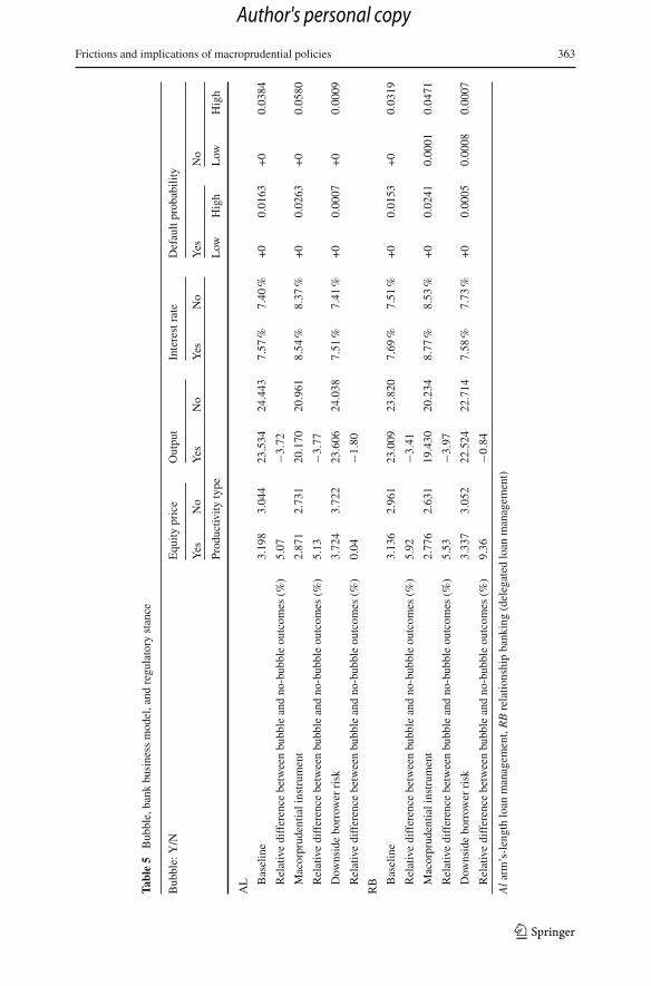
Frictions and implications of macroprudential policies 363
Tabl
e5
Bub
ble,
bank
busi
ness
mod
el,a
ndre
gula
tory
stan
ce
Bub
ble:
Y/N
Equ
itypr
ice
Out
put
Inte
rest
rate
Def
ault
prob
abili
ty
Yes
No
Yes
No
Yes
No
Yes
No
Prod
uctiv
ityty
peL
owH
igh
Low
Hig
h
AL B
asel
ine
3.19
83.
044
23.5
3424
.443
7.57
%7.
40%
+0
0.01
63+
00.
0384
Rel
ativ
edi
ffer
ence
betw
een
bubb
lean
dno
-bub
ble
outc
omes
(%)
5.07
−3.7
2
Mac
orpr
uden
tiali
nstr
umen
t2.
871
2.73
120
.170
20.9
618.
54%
8.37
%+
00.
0263
+0
0.05
80
Rel
ativ
edi
ffer
ence
betw
een
bubb
lean
dno
-bub
ble
outc
omes
(%)
5.13
−3.7
7
Dow
nsid
ebo
rrow
erri
sk3.
724
3.72
223
.606
24.0
387.
51%
7.41
%+
00.
0007
+0
0.00
09
Rel
ativ
edi
ffer
ence
betw
een
bubb
lean
dno
-bub
ble
outc
omes
(%)
0.04
−1.8
0
RB B
asel
ine
3.13
62.
961
23.0
0923
.820
7.69
%7.
51%
+0
0.01
53+
00.
0319
Rel
ativ
edi
ffer
ence
betw
een
bubb
lean
dno
-bub
ble
outc
omes
(%)
5.92
−3.4
1
Mac
orpr
uden
tiali
nstr
umen
t2.
776
2.63
119
.430
20.2
348.
77%
8.53
%+
00.
0241
0.00
010.
0471
Rel
ativ
edi
ffer
ence
betw
een
bubb
lean
dno
-bub
ble
outc
omes
(%)
5.53
−3.9
7
Dow
nsid
ebo
rrow
erri
sk3.
337
3.05
222
.524
22.7
147.
58%
7.73
%+
00.
0005
0.00
080.
0007
Rel
ativ
edi
ffer
ence
betw
een
bubb
lean
dno
-bub
ble
outc
omes
(%)
9.36
−0.8
4
Al
arm
’s-l
engt
hlo
anm
anag
emen
t,R
Bre
latio
nshi
pba
nkin
g(d
eleg
ated
loan
man
agem
ent)
123
Author's personal copy

364 A. Derviz
In all three lending regimes considered (baseline with limited borrower liability andwithout macroprudential capital charges, under macroprudential capital charges, andunder proportional downside risk of the borrower management), the bubble meanshigher equity prices compared to the no-bubble benchmark. The extent of equityovervaluation is somewhat higher under delegated loan management. Average output,on the other hand, is lower under the bubble. A little surprisingly, default probabilitiesare lower compared to the benchmark. This reduction is caused by lower interest ratescharged to high-productivity firms under optimistic sentiment.
Under the arm’s-length bank business model, we observe that in the presence of themacroprudential instrument, bubble removal (restoration of unbiased sentiment) hasa marginally stronger impact on both the equity price and output than in the baselinecase. In the case of a positive bubble, the equity price falls and output rises when thebubble disappears, the same as in the baseline case. The difference between bubble andno-bubble interest rates is also mildly stronger. Unfortunately, this effect is achievedat the cost of reduced economic activity.
Under loan management delegation (relationship banking), the quantitative effectsof the macroprudential capital charges are even less impressive, since, compared tothe baseline, both the output gain and the bubble price correction are smaller. Theadverse absolute impact on output is even more severe than in the AL business model.Apparently, the results of macroprudential policies enacted in a relationship bankingenvironment can be very disappointing due to their inability to exploit the informationaladvantages of delegated loan managers.
On the other hand, enforcing firm manager downside risk, if feasible, could bothreduce the sensitivity of the real economy to the asset price bubble and (the same asin the no-bubble benchmark) improve absolute output levels.
4.4 Bubble containment alternatives: macroprudential versus monetary policy
Having seen the consequences of bubble containment with the introduced macropru-dential instrument, we now compare those consequences with the results of a moretraditional monetary policy tool. We model monetary policy as an exogenous simul-taneous change in the funding cost and the deposit interest rate valuei . That is, whilemonetary policy affects the linear component of banks’ financing costs (irrespectiveof whether this financing comes from deposits or the money market), the macropru-dential tool leaves this linear component unchanged but adjusts the curvature of thenonlinear cost component.
For concreteness, calculations were conducted for our basic limited borrower liabil-ity case and unbiased sentiment. Variations in the value of i resulted in equilibria that,with respect to variables characterizing economic activity, were hard to distinguishfrom the ones obtained from the baseline case by introducing the macroprudential toolof the preceding subsections. In particular, under the used parameterization, we foundthat economic activity returns, more or less, to the baseline level when the macropru-dential policy tested in our simulations is compensated for by a 0.5 % monetary policyeasing (reduction of i). Equivalently, average output, investment, equity prices, and
123
Author's personal copy

Frictions and implications of macroprudential policies 365
Table 6 Macroprudential capital surcharges versus monetary policy tightening
Policy stance: Macroprudential instrument Interest rate hikeIndicator Aggregate Aggregate
AL
q 2.999 3.023
r 0.085 0.085
Default probability
Ld +0 +0
Lu 0.039 0.035
Loss given default 17.193 17.083
Bd 13.304 16.637 13.285 16.574
Bu 19.970 19.862
kd 14.101 16.984 14.106 16.950
ku 19.867 19.795
yd 17.684 21.201 17.690 21.163
yu 24.709 24.637
Bank earnings 0.899965 0.817987
RB
qd 2.756 2.791
qu 3.099 3.119
rd 0.094 0.093
ru 0.081 0.082
Default probability
Ld +0 +0
Lu 0.034 0.031
Loss given default 19.586 18.013
Bd 11.437 16.230 11.534 16.195
Bu 21.022 20.855
kd 12.116 16.540 12.241 16.536
ku 20.964 20.831
yd 15.528 20.717 15.659 20.711
yu 25.906 25.764
Bank earnings 0.8949373 0.816335
Results are shown for the perceived share λ = 0.5 of high-productivity borrowers and no prior bias. Thebase capital surcharge a = 0.01 corresponds to 1 % per first unit of credit uncollateralized by physicalcapital. The foundation stake q0 in firm equity is at level 0.2. The cost of lendable funds (and the depositrate) is 3 % under macroprudential measures and 3.5 % in their absence (the “Interest rate hike” columns).For firms of type #, q# is total equity capital, r# is the borrowing rate, B# is the volume of credit taken, k# isthe total investment in physical capital, y# is expected gross output (when the systemic productivity factortakes its expected value of 1), AL is arm’s-length loan management, RB is relationship banking (delegatedloan management). Borrowers have limited liability
lending rates all react to the macroprudential tool approximately the same way as theywould to a 0.5 % increase in the value of interest rate i . The results of the latter doubleexperiment are shown in Table 6.
123
Author's personal copy

366 A. Derviz
What is the difference, then, between the two policy effects? Inspection of Table 6suggests that there may be a minor increase in default rates and LGD (in the high-productivity, hence risky, borrower segment) under macroprudential tightening com-pared to the monetary policy one, but, given the chosen level of precision, this increaseis barely outside confidence bounds. Much more important is the comparison of effectson bank earnings: they are significantly higher under the macroprudential tighteningthan in the key rate-hike policy case. This indicates that, should the monetary author-ity decide to engage in countercyclical action, banks would prefer macroprudentialactivism to standard monetary policy. This is because monetary policy affects bankfunding costs uniformly and jointly with the firm equity and household deposit mar-kets. On the other hand, the macroprudential tool immediately affects only the lender–borrower link and allows the bank to pass higher funding costs on to the real sectormore easily. This is especially pronounced in the relationship banking case becausethe price discrimination opportunity offered to the loan manager based on his superiorknowledge of the borrower allows the bank to extract higher rents.
Thus, both policy instruments—macroprudential and monetary—contribute super-ficially to suppressing equity price bubbles, but are disappointing in regard to theireffects on other credit excess phenomena such as default probabilities. Quit impor-tantly, their performance on the real economy side of bubble containment is marredby the overall dampening impact on investment and output.
5 Conclusion
I constructed a model of the financial sector that is an interface between conven-tional optimizing general equilibrium macro models and partial equilibrium modelsof financial intermediation driven by information asymmetries. The presence of amacroprudential instrument in this model reduces equilibrium fragility and fulfillsthe formal task of suppressing LGD levels and excessive equity price volatility, butfails to reduce default rates. Most importantly, it entails a uniform and significantincrease in lending rates for all borrowers, resulting in a tangible output loss. Theeffect obtains because the most risky borrower segment, that is, the one targeted bythe policy, is also the one with the highest ex ante performance. Macroprudential cap-ital surcharges mean that those borrowers experience a disproportional, as opposed tothe low-productivity segment, increase in the price of credit. This is a consequence ofan additional transmission channel through physical capital markets: after an initialincrease in the lending rate, banks have to raise the rate even higher because physicalcapital as collateral has become cheaper. This mechanism is at work regardless ofeither the sign or the size of a possible equity bubble.
Both the strength and the robustness of my results with respect to the size of bubblein the physical capital market are due to the mutually reinforcing reactions to shocksby both equity and debt markets. Irrespective of bubbles, the economy demonstratesa high degree of sensitivity of investment and output to small changes in the capitalsurcharge rate.
A monetary policy tool aimed at the same equity bubble, although it mostly impactsthe bank profit side and has very little effect on the producer/borrower side, is slightly
123
Author's personal copy

Frictions and implications of macroprudential policies 367
better at reducing default frequency, but slightly worse than the macroprudential toolwhen it comes to lowering average LGD.
As a further observation, and one worthy of more research, is that the convexmacroprudential capital charge on bank loans helps the investors coordinate on anequilibrium mix of equity and debt financing in situations in which equilibria do notexist in the absence of this instrument. In my model, this is particularly likely to occurwhen firm productivity types are distributed very unevenly or when public economicsentiment is highly biased.
Since macroprudential regulation in its current form affects only lenders, it hasno direct influence on the behavior of borrowers caused by limited liability. How-ever, adverse aggregate consequences of investment decisions by producers who areindifferent between varying degrees of insolvency (do not distinguish between “dead”and “deader” states of the firm that is unable to repay the loan) are more pronouncedthan the consequences due to the absence of a macroprudential response to a bubble.Accordingly, policies able to replicate downside risk on the borrower side are likely tobe the next fundamental challenge for financial regulation. The resulting equilibria in amodified “proportional liability” regime also entail reduced default rates for the mostrisky borrowers, compared to the pure limited liability case. More generally, thereseem to be limits, in terms of economic activity and ex ante welfare costs, to promot-ing financial stability through policies directed at credit providers. At the same time,policies with the same ultimate objective of systemic risk containment, but directed atcredit consumers, continue to be largely unexplored (let alone exploited). My resultsindicate that the potential benefit gained by reorienting from regulating credit supplyto educating credit demand may be worthwhile, notwithstanding numerous implemen-tation difficulties.
Acknowledgments I thank seminar participants at the Czech National Bank and the European Cen-tral Bank MARS network, participants at the 2011 Swiss Society for Financial Market Research AnnualConference, and an anonymous referee for helpful comments.
References
Angelini, P., Neri, S., Panetta, F.: Grafting Macroprudential Policies in a Macroeconomic Framework.Choice of Optimal Instruments and Interaction with Monetary Policy. Mimeo, Bank of Italy (2010)
Aoki, K., Proudman, J., Vlieghe, G.: House prices, consumption, and monetary policy: a financial acceleratorapproach. J Financ Intermed 13(5), 414–435 (2004)
Bernanke, B.S., Gertler, M., Gilchrist, S.: The financial accelerator in a quantitative business cycle frame-work. In: Taylor, J.B., Woodford, M. (eds.) Handbook of Macroeconomics, 1st edn, chap. 21, vol. 1,pp. 1341–1393. Elsevier, Amsterdam (1999)
Besanko, D., Thakor, A.V.: Competitive equilibrium in the credit market under asymmetric information.J Econ Theory 42, 167–182 (1987)
Blum, J., Hellwig, M.: The macroeconomic implications of capital adequacy requirements for banks. EurEcon Rev 39(3–4), 739–749 (1995)
Bonaccorsi di Patti, E., Dell’Ariccia, G.: Bank competition and firm creation. J Money Credit Bank 36(2),225–251 (2004)
Borio, C.: Towards a Macroprudential Framework for Financial Supervision and Regulation? BIS WP No.128 (February) (2003)
Christiano, L.J., Motto, R., Rostagno, M.: Shocks, structures or policies? The euro area and the US after2001. J Econ Dyn Control 32(13), 2476–2506 (2008)
123
Author's personal copy

368 A. Derviz
Covas, F., Fujita, S.: Procyclicality of capital requirements in a general equilibrium model of liquiditydependence. Int J Cent Bank 6(5), 137–173 (2010)
Dell’Ariccia, G., Marquez, R.: Information and bank credit allocation. J Financ Econ 72, 185–214 (2004)de Walque, G., Pierrard, O., Rouabah, A.: Financial (in)stability, supervision and liquidity injections:
a dynamic general equilibrium approach. Econ. J. 120, 1234–1261 (2010)Diamond, D.: Financial intermediation and delegated monitoring. R Econ Stud 51(3), 393–414 (1984)Diamond, D., Rajan, R.: A theory of bank capital. J Finance 55(6), 2431–2465 (2000)Donaldson, J.B., Gershun, N., Giannoni, M.P.: Some Unpleasant General Equilibrium Implications of
Executive Incentive Compensation Contracts. NBER Working Paper Series, vol. w15165 (July) (2009)He, Z., Krishnamurthy, A.: Intermediary Asset Pricing, Working Paper. Chicago Booth and Northwestern
University (2010)Hui, O.-Y.: Optimal contracts in a continuous-time delegated portfolio management problem. Rev Financ
Stud 16(1), 173–208 (2003)Iacoviello, M.: House prices, borrowing constraints, and monetary policy in the business cycle. Am Econ
Rev 95(3), 739–764 (2005)International Monetary Fund (IMF): Lessons for monetary policy from asset price fluctuations. In: World
Economic Outlook, Chapter 3 (October) (2009)Kraft, H., Korn, R.: Continuous-time delegated portfolio management with homogeneous expectations: can
an agency conflict be avoided? Financ Mark Portf Manag 22(1), 67–90 (2008)Mendoza, E.: Sudden stops, financial crises, and leverage. Am Econ Rev 100, 1941–1966 (2010)Monacelli, T.: New Keynesian models, durable goods, and collateral. J Monet Econ 56, 242–254 (2009)Rajan, R.: Insiders and outsiders: the choice between informed and arm’s-length debt. J Finance 47, 1367–
1400 (1992)Repullo, R., Suarez, J.: The Procyclical Effects of Bank Capital Regulation, WP 2010–29S. Tilburg Uni-
versity, Center for Economic Research (2010)Santomero, A.: Modeling the banking firm: a survey. J Money Credit Bank 16(5), 576–602 (1984)Saunders, A., Walter, I.: Financial architecture, systemic risk, and universal banking. Financ Mark Portf
Manag 26(1), 39–59 (2012)Sharpe, S.: Asymmetric information, bank lending, and implicit contracts: a theoretical model of customer
relationship. J Finance 45, 1069–1087 (1990)Stiglitz, J., Weiss, A.: Credit rationing with imperfect information. Am Econ Rev 71(3), 393–410 (1981)Townsend, R.M.: Optimal contracts and competitive markets with costly state verification. J Econ Theory
22, 265–293 (1979)
Author Biography
Alexis Derviz is a Principal Economist in charge of a team of international economy analysts at the CzechNational Bank. He received a Ph.D. in mathematical physics from the Leningrad (St. Petersburg) StateUniversity in Russia. He later studied economics at Charles University in Prague, Czech Republic, andtaught industrial organization and international finance at the graduate school of economics of that uni-versity. He then joined the Czech National Bank to lead a research team on international monetary issues.He contributed to and co-edited several books on economies in transition, later authored a number of ref-ereed journal articles on asset pricing, exchange rates and international banking.
123
Author's personal copy


![library.utia.cas.czlibrary.utia.cas.cz/separaty/2018/MTR/noguera-0486421.pdf · JID:FSS AID:7364 /FLA [m3SC+; v1.279; Prn:12/02/2018; 14:20] P.1(1-16) Available online at ScienceDirect](https://img.pdfslide.us/doc/110x75/603ae43483b01951a17f2a65/jidfss-aid7364-fla-m3sc-v1279-prn12022018-1420-p11-16-available.jpg)