Embed Size (px)
Citation preview
Institute of Economic Studies, Faculty of Social Sciences
Charles University in Prague
Volatility extraction using the Kalman filter
Alexandr Kuchynka
IES Working Paper: 10/2008

Institute of Economic Studies, Faculty of Social Sciences,
Charles University in Prague
[UK FSV – IES]
Opletalova 26 CZ-110 00, Prague
E-mail : [email protected] http://ies.fsv.cuni.cz
Institut ekonomický ch studií Fakulta sociálních věd
Univerzita Karlova v Praze
Opletalova 26 110 00 Praha 1
E-mail : [email protected]
http://ies.fsv.cuni.cz
Disclaimer: The IES Working Papers is an online paper series for works by the faculty and students of the Institute of Economic Studies, Faculty of Social Sciences, Charles University in Prague, Czech Republic. The papers are peer reviewed, but they are not edited or formatted by the editors. The views expressed in documents served by this site do not reflect the views of the IES or any other Charles University Department. They are the sole property of the respective authors. Additional info at: [email protected] Copyright Notice: Although all documents published by the IES are provided without charge, they are licensed for personal, academic or educational use. All rights are reserved by the authors. Citations: All references to documents served by this site must be appropriately cited. Bibliographic information: Kuchynka, A. (2008). “ Volatility extraction using the Kalman filter ” IES Working Paper 10/2008. IES FSV. Charles University.
This paper can be downloaded at: http://ies.fsv.cuni.cz
Volatility extraction using the Kalman filter
Alexandr Kuchynka#
# IES, Charles University Prague,
Institute of Information Theory and Automation of the ASCR, Faculty of Economics, University of West Bohemia in Pilsen
E-mail: [email protected]
June 2008 Abstract: This paper focuses on the extraction of volatility of financial returns. The volatility process is modeled as a superposition of two autoregressive processes which represent the more persistent factor and the quickly mean-reverting factor. As the volatility is not observable, the logarithm of the daily high-low range is employed as its proxy. The estimation of parameters and volatility extraction are performed using a modified version of the Kalman filter which takes into account the finite sample distribution of the proxy. Keywords: volatility, stochastic volatility models, Kalman filter, volatility proxy JEL: C22,G15. Acknowledgements: This research was supported by Czech Science Foundation GACR under Grant Nr. 402/07/0465 and Ministry of Education of the Czech Republic within the Center for Basic Research in Dynamic Economics and Econometrics (LC06075).
1
1. Introduction
Modelling financial data comprises several issues, the most important being a proper specification of the time-varying variance of financial returns, so called volatility. As the variance of returns is used as a measure of risk, the importance of an adequate characterization of volatility is obvious in the areas of risk management or portfolio optimization. Another application arises in the context of option pricing. In the original Black-Scholes setting, the risk is quantified by a constant volatility parameter. If the true variance of the financial asset is time-varying rather then constant, the pricing formula has to be modified correspondingly.
There exist two prominent approaches to deal with volatility: GARCH and stochastic volatility (SV) approaches. The GARCH model (Engle, 1982, Bollerslev, 1986) focuses on capturing the clustering of volatility in returns when the conditional variance at time t is modelled as a deterministic function of lagged values of conditional variances and squared returns. On the other hand, the stochastic volatility models understand the time-varying variance as a stochastic process which can be a continuous-time diffusion (Hull and White, 1987) or a more general Lé vy process (Barndorff-Nielsen and Shepard, 2001). Stochastic volatility models are typically formulated in the state space form and they are intimately related to the problem of signal extraction. It is well-known (see for instance Hamilton, 1994) that for linear system with Gaussian innovations the Kalman filter offers an optimal way (in the sense of minimizing mean squared errors) for sequentially updating a linear projection.
The paper is organized as follows: in the second chapter, we introduce the concept of the volatility proxy along the lines of de Vilder and Visser (2007) which represents an useful framework for assessing the quality of such proxies. Typical representants of volatility proxies are the high-low range and the absolute daily return because they are constructed from the easily available quaternion „high-low-open-close“ price. Since it turns out that logarithm of daily range (hereafter log range) has substantially lower variance than logarithm of absolute return and is nearly Gaussian, we will concentrate on this proxy. Although the asymptotic distribution of the log range has been studied in detail in Alizadeh et al. (2002), less attention has been paid to its finite sample counterpart. In particular, due to the discretization error, the mean and variance of the distribution vary with the number of points

2
in the grid over which minima and maxima are taken. We study the sensitivity of first four moments on the number of observations using a Monte Carlo simulation.
In the third chapter we suggest a modification of the standard Kalman filter algorithm
which uses finite sample mean and variance of the log range as input. Finally in the fourth chapter, we apply our methodology to the data from the Prague Stock Exchange. 2. Measuring volatility using proxies
In our setup, we make use of the framework developed in de Vilder and Visser (2007) which is particularly useful when dealing with proxies for unobserved volatility. Recall that discrete time models typically exhibit a product structure
t t tr s Z= (1) where the observed return for day t tr is described as a product of some positive scale factor
ts and i.i.d. innovation tZ .
It is useful to consider a continuous time version of (1) with independent copies { }tΨ of some stochastic process Ψ in place of i.i.d. noise { }tZ :
( ) ( ) [ ], 0,1t t tR sϑ ϑ ϑ= Ψ ∈ (2) Thus, the cumulated log return tR is just a scaled version of some stochastic process tΨ which can be a Wiener process (in the simpliest setup) or a more complex process capturing intraday seasonality or jumps. Formally, we suppose that Ψ is a cà dlà g (right continuous with left limits) proces on [ ]0,1 , left continuous at 1. For identification purposes we assume
that Ψ is standardized, i.e. ( ) ( )( )1 0, var 1 1EΨ = Ψ = . The time ϑ runs from the opening until the closing of the trading day, the overnight return from day t-1 to t is given by
( )0t ts Ψ . Daily close-to-close return then becomes
( ) ( )1 1t t t tr R s= = Ψ (3)
In order to compare this approach with the usual stochastic volatility models, suppose that Ψ is a diffusion obeying
( ) ( ) ( )d v dBϑ ϑ ϑΨ = (4) with instantaneous stochastic volatility ( )v ϑ . The cumulated log return process then follows
( ) ( ) ( ) ( ) ( )t t t tdR s v dB dBϑ ϑ ϑ σ ϑ ϑ= ≡ (5)

3
Thus, the local volatility ( )tσ ϑ can be decomposed into a daily scale factor ts and an
independent component ( )tv ϑ capturing intraday effects.
The daily scale factor ts is not directly observable and therefore has to be approximated by some random variable which serves as its proxy. A good proxy should exhibit large correlation with ts . The notion of a proxy can be formalized as follows: Definition (de Vilder and Visser, 2007). Let H be a measurable functional [ )0,D → ∞
defined on a linear subspace D of [ ]0,1D (Skorohod space of cà dlà g functions on [ ]0,1 left continuous in 1) and DΨ ∈ a.s. Assume (i) H is positively homogeneous, i.e.
( ) ( ) [ ), 0, ,H H Dα α αΨ = Ψ ∈ ∞ Ψ ∈ (ii) ( ) 0H Ψ > a.s. Then 1. H is called a proxy functional. 2. the random variable tΠ is a proxy for the daily scale factor ts :
( ) ( )t t t t t t tH s s H s VΠ = Ψ = Ψ ≡ ,
tV is called a nuisance proxy.
An additive measurement equation is obtained by taking logs:
( )log log log log log log logt t t t t t ts V s E V V E VΠ = + = + + − (6) This equation decomposes the log proxy into a sum of log-volatility, a constant bias and measurement errors
log logt t tu V E V≡ − A quality of a proxy is determined by the variance of the measurement errors ( )2 var tuλ ≡ .
In the sequel, we will focus on approximating log ts and for simplicity we will use the word proxy in the meaning of log tΠ . Typical examples of such proxies include log range
[ ]( )
[ ]( )
0,10,1log sup inft tR R
ϑϑϑ ϑ
∈∈
−
(7)
4
and log absolute return
( ) ( )log 1 0t tR R− . (8)
The asymptotic distribution of both proxies has been studied in Alizadeh et al. (2002). Based on the result of Feller (1951), they find out that if Ψ is a driftless standardized Wiener process, ( ) ( )( )log sup infϑ ϑΨ − Ψ can be well aproximated by the normal distribution with
mean 0.43 and variance 0.084. On the other hand, the variance of ( ) ( )log 1 0Ψ − Ψ is much
higher (equal to 2 / 8 1.23π ! ) and the proxy is left skewed and leptokurtic. For this reason, the use of the log range instead of the log absolute return is highly recommended.
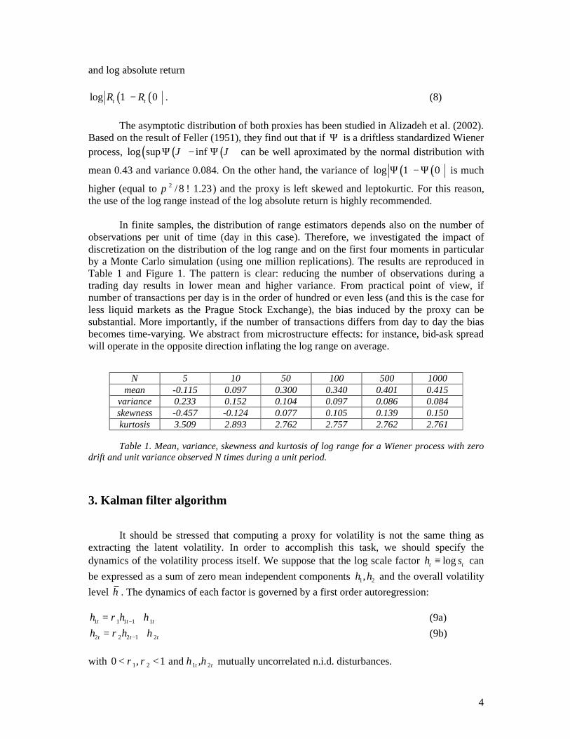
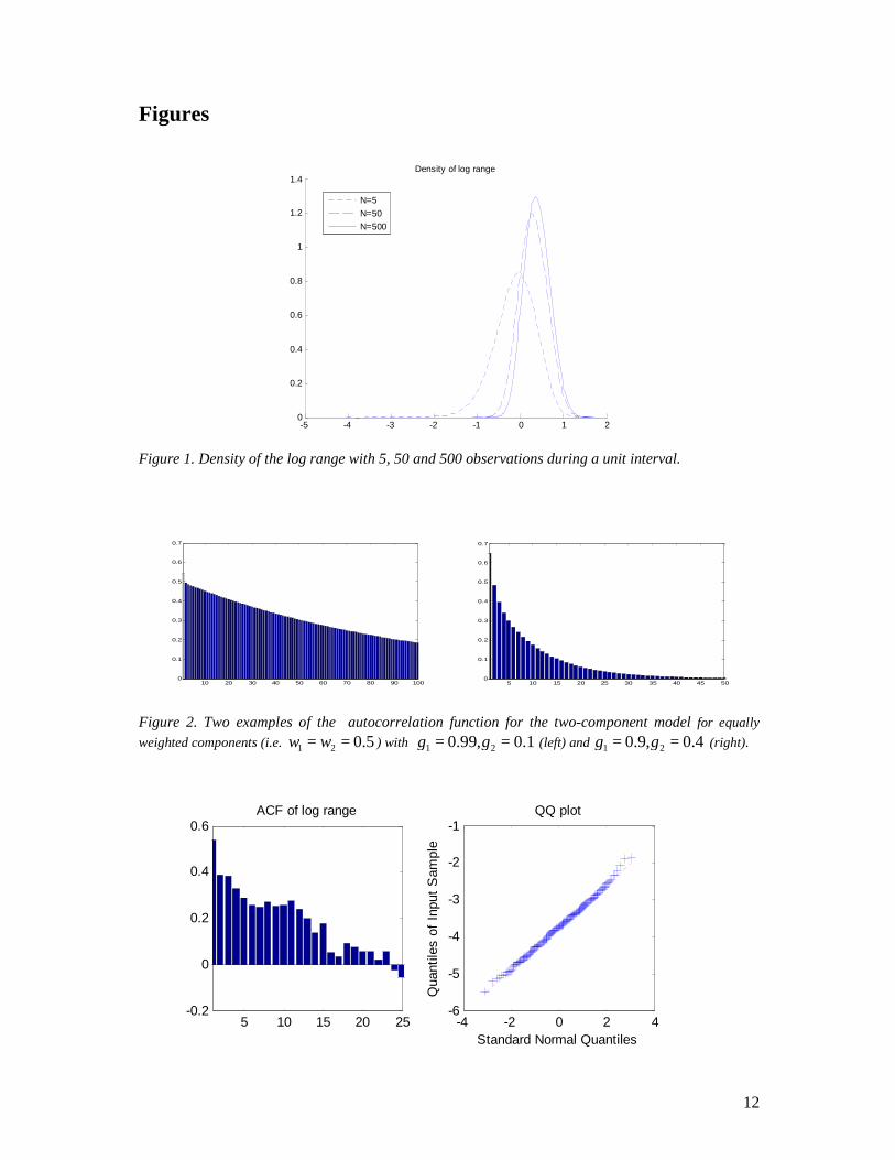
In finite samples, the distribution of range estimators depends also on the number of observations per unit of time (day in this case). Therefore, we investigated the impact of discretization on the distribution of the log range and on the first four moments in particular by a Monte Carlo simulation (using one million replications). The results are reproduced in Table 1 and Figure 1. The pattern is clear: reducing the number of observations during a trading day results in lower mean and higher variance. From practical point of view, if number of transactions per day is in the order of hundred or even less (and this is the case for less liquid markets as the Prague Stock Exchange), the bias induced by the proxy can be substantial. More importantly, if the number of transactions differs from day to day the bias becomes time-varying. We abstract from microstructure effects: for instance, bid-ask spread will operate in the opposite direction inflating the log range on average.
N 5 10 50 100 500 1000 mean -0.115 0.097 0.300 0.340 0.401 0.415
variance 0.233 0.152 0.104 0.097 0.086 0.084 skewness -0.457 -0.124 0.077 0.105 0.139 0.150 kurtosis 3.509 2.893 2.762 2.757 2.762 2.761
Table 1. Mean, variance, skewness and kurtosis of log range for a Wiener process with zero
drift and unit variance observed N times during a unit period. 3. Kalman filter algorithm
It should be stressed that computing a proxy for volatility is not the same thing as extracting the latent volatility. In order to accomplish this task, we should specify the dynamics of the volatility process itself. We suppose that the log scale factor logt th s≡ can be expressed as a sum of zero mean independent components 1 2,h h and the overall volatility level h . The dynamics of each factor is governed by a first order autoregression:
1 1 1 1 1t t th hρ η−= + (9a)
2 2 2 1 2t t th hρ η−= + (9b) with 1 20 , 1ρ ρ< < and 1 2,t tη η mutually uncorrelated n.i.d. disturbances.
5
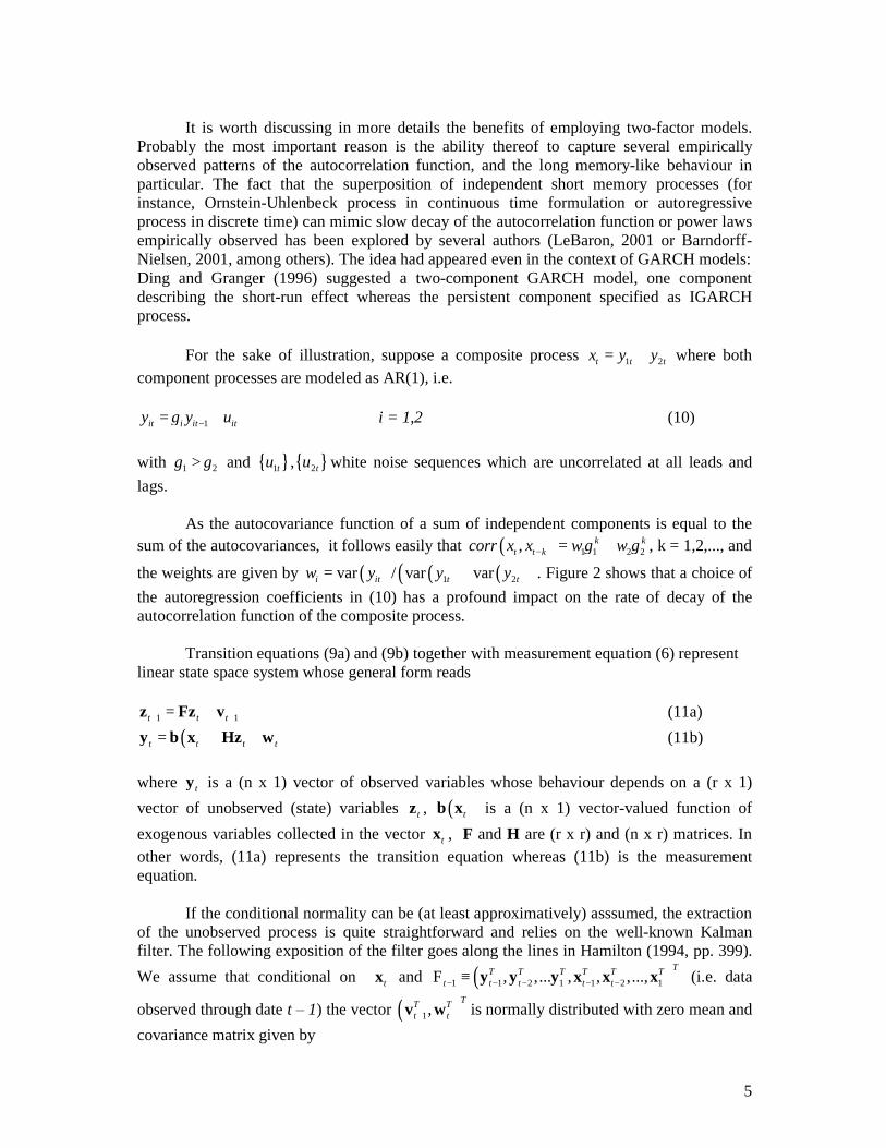
It is worth discussing in more details the benefits of employing two-factor models.
Probably the most important reason is the ability thereof to capture several empirically observed patterns of the autocorrelation function, and the long memory-like behaviour in particular. The fact that the superposition of independent short memory processes (for instance, Ornstein-Uhlenbeck process in continuous time formulation or autoregressive process in discrete time) can mimic slow decay of the autocorrelation function or power laws empirically observed has been explored by several authors (LeBaron, 2001 or Barndorff-Nielsen, 2001, among others). The idea had appeared even in the context of GARCH models: Ding and Granger (1996) suggested a two-component GARCH model, one component describing the short-run effect whereas the persistent component specified as IGARCH process.
For the sake of illustration, suppose a composite process 1 2t t tx y y= + where both
component processes are modeled as AR(1), i.e.
1it i it ity y uγ −= + i = 1,2 (10) with 1 2γ γ> and { } { }1 2,t tu u white noise sequences which are uncorrelated at all leads and lags.
As the autocovariance function of a sum of independent components is equal to the sum of the autocovariances, it follows easily that ( ) 1 1 2 2, k k
t t kcorr x x w wγ γ− = + , k = 1,2,..., and
the weights are given by ( ) ( ) ( )( )1 2var / var vari it t tw y y y= + . Figure 2 shows that a choice of the autoregression coefficients in (10) has a profound impact on the rate of decay of the autocorrelation function of the composite process.
Transition equations (9a) and (9b) together with measurement equation (6) represent linear state space system whose general form reads
1 1t t t+ += +z Fz v (11a)
( )t t t t= + +y b x Hz w (11b) where ty is a (n x 1) vector of observed variables whose behaviour depends on a (r x 1) vector of unobserved (state) variables tz , ( )tb x is a (n x 1) vector-valued function of exogenous variables collected in the vector tx , F and H are (r x r) and (n x r) matrices. In other words, (11a) represents the transition equation whereas (11b) is the measurement equation.
If the conditional normality can be (at least approximatively) asssumed, the extraction of the unobserved process is quite straightforward and relies on the well-known Kalman filter. The following exposition of the filter goes along the lines in Hamilton (1994, pp. 399). We assume that conditional on tx and ( )1 1 2 1 1 2 1, ,... , , ,...,
TT T T T T Tt t t t t− − − − −≡ y y y x x xF (i.e. data
observed through date t – 1) the vector ( )1,TT T
t t+v w is normally distributed with zero mean and covariance matrix given by
6
( )t
Q 00 R x
(12)
The exogenous vector tx has been introduced in order to deal with small sample effects which have influence on the bias and the variance of the proxy.
Further, suppose that ( )1 | 1 | 1| , ,t t t t t t tN− − −z x z P!F . Then the distribution of the vector
( ),TT T
t tz y conditional on tx and 1t−F is normal with mean vector
( )( )| 1 | 1,TT T T T
t t t t t− −+z b x z H (13) and covariance matrix
| 1 | 1
| 1
Tt t t t
t t t
− −
−
P P HHP V
(14)
with ( )| 1
Tt t t t−≡ +V HP H R x .
For updating the inference about the current value of the state variables tz as a new
observation of ty becomes available we use the fact that
( )1 | || , , | ,t t t t t t t t t tN− ≡z y x z z P!F F (15) where
( )( )1| | 1 | 1 | 1
Tt t t t t t t t t t t
−− − −= + − −z z P H V y b x Hz (16)
1| | 1 | 1 | 1
Tt t t t t t t t t
−− − −= −P P P H V HP (17)
The matrix 1| 1
Tt t t t
−−≡K P H V is often called the (Kalman) gain matrix or weight matrix
and expresses the weights of innovations ( ) | 1t t t t−− −y b x Hz in producing the filtered estimate of the state variable |t tz . Roughly speaking, if the variance of the measurement noise is high, the weights attributed to the recent observation are relatively low and vice versa. In the standard Kalman filter case (with constant coefficients) under suitable conditions the sequence of matrices{ }tK converges to a fixed, steady-state matrix (Proposition 13.1, Hamilton, 1994). If the covariance matrix of the measurement noise R is time-dependent rather than constant then { }tK will fluctuate as well.
Subsequently, the conditional distribution of the state vector at time t+1 given the
observations known through date t, i.e. ( )1 1| 1|| ,t t t t t tN+ + +z z P!F where
7
1| |t t t t+ =z Fz (18)
1| |T
t t t t+ = +P FP F Q (19) The sample log likelihood function reads (after omitting constant terms)
( )( ) ( )( )1| 1 | 1
1 1
1 1log2 2
T T Tt t t t t t t t t t
t t
−− −
= =
− − − − − −∑ ∑V y b x Hz V y b x Hz (20)
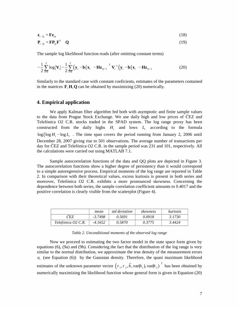
Similarly to the standard case with constant coeficients, estimates of the parameters contained in the matrices , ,F H Q can be obtained by maximizing (20) numerically. 4. Empirical application We apply Kalman filter algorithm fed both with asymptotic and finite sample values to the data from Prague Stock Exchange. We use daily high and low prices of ČEZ and Telefó nica O2 C.R. stocks traded in the SPAD system. The log range proxy has been constructed from the daily highs tH and lows tL according to the formula
( )log log logt tH L− . The time span covers the period running from January 2, 2006 until December 28, 2007 giving rise to 501 observations. The average number of transactions per day for ČEZ and Telefó nica O2 C.R. in the sample period was 231 and 101, respectively. All the calculations were carried out using MATLAB 7.1.
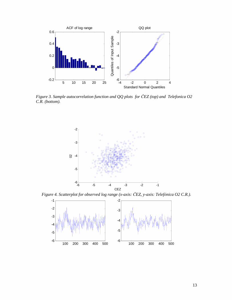
Sample autocorrelation functions of the data and QQ plots are depicted in Figure 3.
The autocorrelation functions show a higher degree of persistency than it would correspond to a simple autoregressive process. Empirical moments of the log range are reported in Table 2. In comparison with their theoretical values, excess kurtosis is present in both series and moreover, Telefó nica O2 C.R. exhibits a more pronounced skewness. Concerning the dependence between both series, the sample correlation coefficient amounts to 0.4017 and the positive correlation is clearly visible from the scatterplot (Figure 4).
mean std deviation skewness kurtosis ČEZ -3.7498 0.5691 0.0918 3.1730
Telefó nica O2 C.R. -4.1652 0.5870 0.3775 3.4424
Table 2. Unconditional moments of the observed log range
Now we proceed to estimating the two factor model in the state space form given by equations (6), (9a) and (9b). Considering the fact that the distribution of the log range is very similar to the normal distribution, we approximate the true density of the measurement errors
tu (see Equation (6)) by the Gaussian density. Therefore, the quasi maximum likelihood
estimates of the unknown parameter vector ( )1 2 1 2, , , var( ), var( )T
hρ ρ η η has been obtained by numerically maximizing the likelihood function whose general form is given in Equation (20)
8
with respect to these parameters. As stated above, we employ two versions of the Kalman filter:
(i) Kalman filter with constant coeficients in the measurement equation corresponding to the asymptotic values, that is ( )tb x = 0.43 and ( )tR x = 0.084 in the notation of the Chapter 3, (ii) Kalman filter with time-varying coefficients; the finite sample mean and variance have been computed by means of Monte Carlo simulation (cf. Table 1).
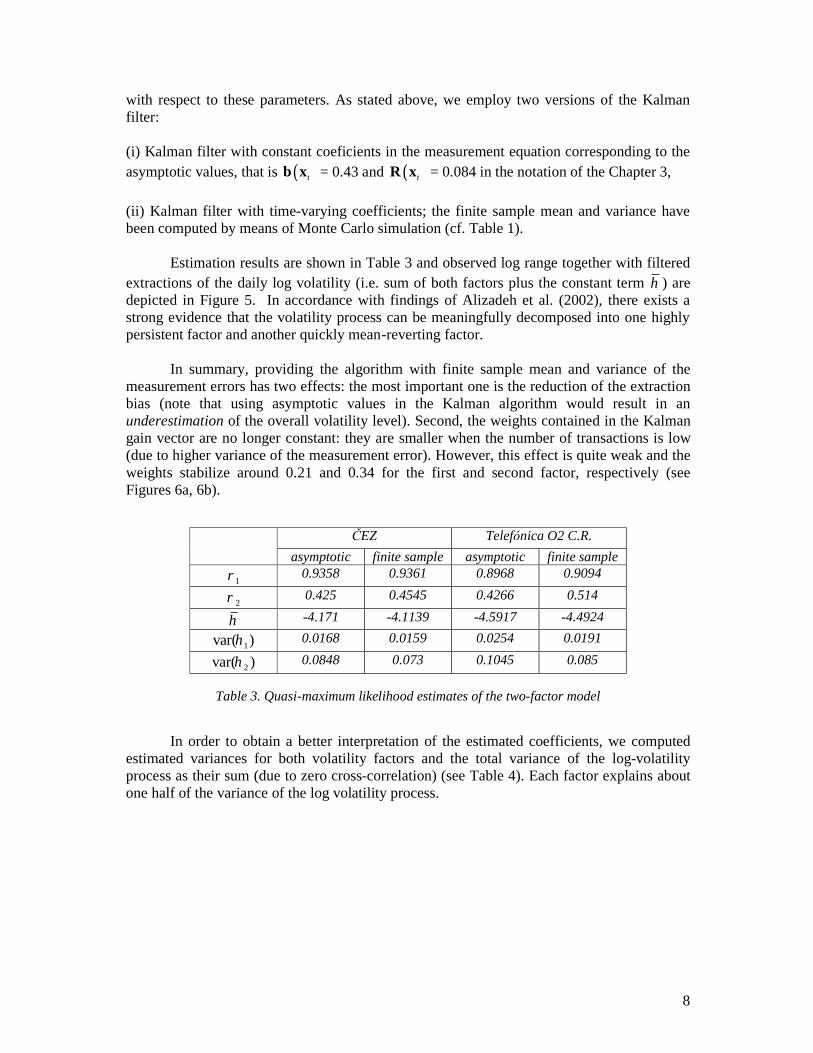
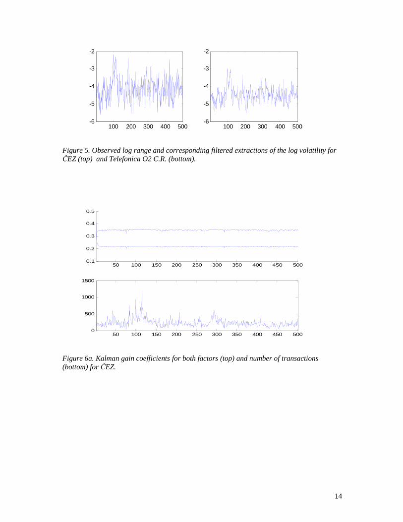
Estimation results are shown in Table 3 and observed log range together with filtered extractions of the daily log volatility (i.e. sum of both factors plus the constant term h ) are depicted in Figure 5. In accordance with findings of Alizadeh et al. (2002), there exists a strong evidence that the volatility process can be meaningfully decomposed into one highly persistent factor and another quickly mean-reverting factor.
In summary, providing the algorithm with finite sample mean and variance of the
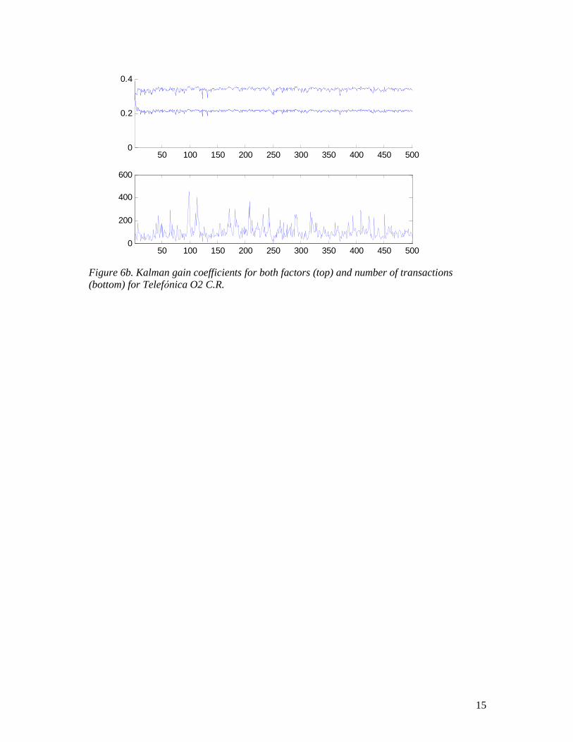
measurement errors has two effects: the most important one is the reduction of the extraction bias (note that using asymptotic values in the Kalman algorithm would result in an underestimation of the overall volatility level). Second, the weights contained in the Kalman gain vector are no longer constant: they are smaller when the number of transactions is low (due to higher variance of the measurement error). However, this effect is quite weak and the weights stabilize around 0.21 and 0.34 for the first and second factor, respectively (see Figures 6a, 6b).
ČEZ Telefó nica O2 C.R.
asymptotic finite sample asymptotic finite sample 1ρ 0.9358 0.9361 0.8968 0.9094
2ρ 0.425 0.4545 0.4266 0.514
h -4.171 -4.1139 -4.5917 -4.4924
1var( )η 0.0168 0.0159 0.0254 0.0191
2var( )η 0.0848 0.073 0.1045 0.085
Table 3. Quasi-maximum likelihood estimates of the two-factor model
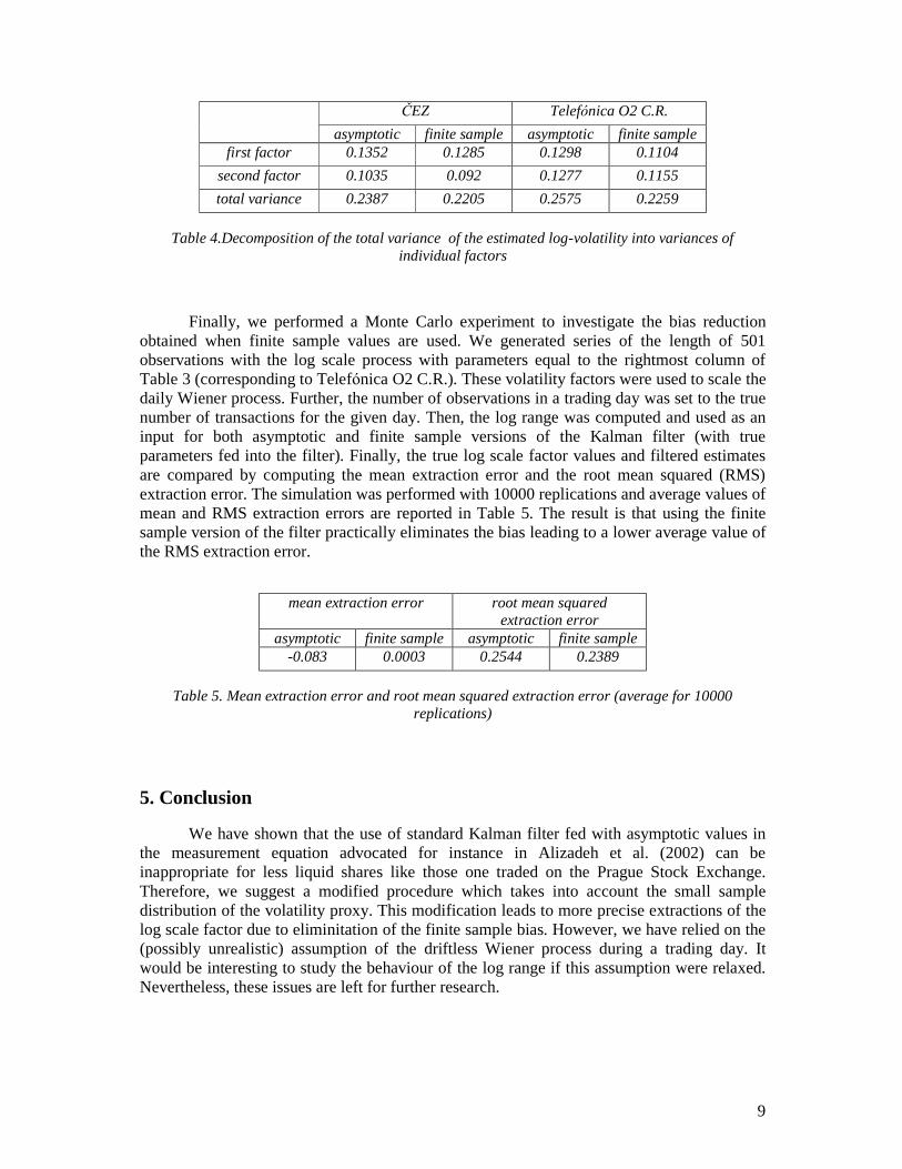
In order to obtain a better interpretation of the estimated coefficients, we computed estimated variances for both volatility factors and the total variance of the log-volatility process as their sum (due to zero cross-correlation) (see Table 4). Each factor explains about one half of the variance of the log volatility process.
9
ČEZ Telefó nica O2 C.R.
asymptotic finite sample asymptotic finite sample first factor 0.1352 0.1285 0.1298 0.1104
second factor 0.1035 0.092 0.1277 0.1155 total variance 0.2387 0.2205 0.2575 0.2259
Table 4.Decomposition of the total variance of the estimated log-volatility into variances of
individual factors
Finally, we performed a Monte Carlo experiment to investigate the bias reduction obtained when finite sample values are used. We generated series of the length of 501 observations with the log scale process with parameters equal to the rightmost column of Table 3 (corresponding to Telefó nica O2 C.R.). These volatility factors were used to scale the daily Wiener process. Further, the number of observations in a trading day was set to the true number of transactions for the given day. Then, the log range was computed and used as an input for both asymptotic and finite sample versions of the Kalman filter (with true parameters fed into the filter). Finally, the true log scale factor values and filtered estimates are compared by computing the mean extraction error and the root mean squared (RMS) extraction error. The simulation was performed with 10000 replications and average values of mean and RMS extraction errors are reported in Table 5. The result is that using the finite sample version of the filter practically eliminates the bias leading to a lower average value of the RMS extraction error.
mean extraction error root mean squared extraction error
asymptotic finite sample asymptotic finite sample -0.083 0.0003 0.2544 0.2389
Table 5. Mean extraction error and root mean squared extraction error (average for 10000
replications) 5. Conclusion
We have shown that the use of standard Kalman filter fed with asymptotic values in the measurement equation advocated for instance in Alizadeh et al. (2002) can be inappropriate for less liquid shares like those one traded on the Prague Stock Exchange. Therefore, we suggest a modified procedure which takes into account the small sample distribution of the volatility proxy. This modification leads to more precise extractions of the log scale factor due to eliminitation of the finite sample bias. However, we have relied on the (possibly unrealistic) assumption of the driftless Wiener process during a trading day. It would be interesting to study the behaviour of the log range if this assumption were relaxed. Nevertheless, these issues are left for further research.
10
References ALIZADEH, S. - BRANDT, M. - DIEBOLD, F. (2002): Range-based estimation of stochastic volatility models. Journal of Finance 57, pp. 1047–1091. ANDERSEN, T.G. - BOLLERSLEV, T. - DIEBOLD, F.X. - LABYS, P. (2001): The distribution of realized exchange rate volatility. Journal of the American Statistical Association 96, pp. 42–55. BARNDORFF-NIELSEN, O. (2001): Superposition of Ornstein-Uhlenbeck type processes. Theory Prob. Its Appl. 45, pp. 175-194. BARNDORFF-NIELSEN, O. E. – SHEPARD, N. (2001): Non-Gaussian Ornstein-Uhlenbeck-based models and some of their uses in financial economic.. Journal of the Royal Statistical Society, Series B 63, pp. 167-241. BOLLERSLEV, T. (1986): Generalized autoregressive conditional heteroskedasticity. Journal of Econometrics 31, pp. 307–327. CHRISTENSEN, K. - PODOLSKIJ, M. (2006): Realized range-based estimation of integrated variance, Journal of Econometrics (forthcoming). DE VILDER, R.G. – VISSER, M.P. (2007): Volatility Proxies for Discrete Time Models, MPRA Paper 4917, University Library of Munich, Germany. DING, Z. – GRANGER, C.W.J. (1996): Modeling volatility persistence of speculative returns: a new approach. Journal of Econometrics, 73, no 1, pp. 185-215. ENGLE, R.F. (1982): Autoregressive conditional heteroscedasticity with estimates of the variance of United Kingdom inflation. Econometrica 50, pp. 987–1007. FELLER, W. (1951): The asymptotic distribution of the range of sums of independent random variables . Annals of Mathematical Statistics, 22, pp. 427-432. GARMAN, M. – KLASS, M.J. (1980): On the estimation of security price volatilities from historical data. Journal of Business, 53, pp. 67-78. HAMILTON, J. (1994): Time Series Analysis. Princeton, Princeton University Press. HARVEY, A.C. – RUIZ, E. – SHEPARD, N. (1994): Multivariate stochastic variance models. Rev. Economic Studies, 61, pp. 247-264. HULL, J. – WHITE, A. (1987): The pricing of options on assets with stochastic volatilities. Journal of Finance 42, pp. 281 - 300. LEBARON, B. (2001): Stochastic volatility as a simple generator of apparent financial power laws and long memory. Quantitative Finance, Vol 1, No 6, pp. 621-31. MARTENS, M. – VAN DIJK, D. (2007): Measuring volatility with the realized range. Journal of Econometrics, 138, pp. 181-207. PARKINSON, M. (1980): The extreme value method for estimating the variance of the rate of return. Journal of Business, 53(1), pp. 61-65. ROGERS, L. C. G. - SATCHELL, S. E. (1991): Estimating variances from high, low, and closing prices, Annals of Applied Probability 1(4), pp. 504–512. RUIZ, E. (1994): Quasi-maximum likelihood estimation of stochastic volatility models. Journal of Econometrics, 63, pp. 289 − 306.

11
TAYLOR, S. J. (1982): Financial returns modelled by the product of two stochastic processes - a study of daily sugar prices 1961-79. In O. D. Anderson (ed.), Time Series Analysis: Theory and Practice, 1, pp. 203-226. Amsterdam: North-Holland.
12
Figures
-5 -4 -3 -2 -1 0 1 20
0.2
0.4
0.6
0.8
1
1.2
1.4Density of log range
N=5N=50N=500
Figure 1. Density of the log range with 5, 50 and 500 observations during a unit interval.
10 20 30 40 50 60 70 80 90 1000
0.1
0.2
0.3
0.4
0.5
0.6
0.7
5 10 15 20 25 30 35 40 45 50
0
0.1
0.2
0.3
0.4
0.5
0.6
0.7
Figure 2. Two examples of the autocorrelation function for the two-component model for equally weighted components (i.e. 1 2 0.5w w= = ) with 1 20.99, 0.1γ γ= = (left) and 1 20.9, 0.4γ γ= = (right).
5 10 15 20 25-0.2
0
0.2
0.4
0.6ACF of log range
-4 -2 0 2 4-6
-5
-4
-3
-2
-1
Standard Normal Quantiles
Qua
ntile
s of
Inpu
t Sam
ple
QQ plot
13
5 10 15 20 25-0.2
0
0.2
0.4
0.6ACF of log range
-4 -2 0 2 4-6
-5
-4
-3
-2
Standard Normal Quantiles
Qua
ntile
s of
Inpu
t Sam
ple
QQ plot
Figure 3. Sample autocorrelation function and QQ plots for ČEZ (top) and Telefonica O2 C.R. (bottom).
-6 -5 -4 -3 -2 -1-6
-5
-4
-3
-2
CEZ
02
Figure 4. Scatterplot for observed log range (x-axis: ČEZ, y-axis: Telefó nica O2 C.R.).
100 200 300 400 500-6
-5
-4
-3
-2
-1
100 200 300 400 500-6
-5
-4
-3
-2
14
100 200 300 400 500-6
-5
-4
-3
-2
100 200 300 400 500-6
-5
-4
-3
-2
Figure 5. Observed log range and corresponding filtered extractions of the log volatility for ČEZ (top) and Telefonica O2 C.R. (bottom).
50 100 150 200 250 300 350 400 450 5000.1
0.2
0.3
0.4
0.5
50 100 150 200 250 300 350 400 450 5000
500
1000
1500
Figure 6a. Kalman gain coefficients for both factors (top) and number of transactions (bottom) for ČEZ.
15
50 100 150 200 250 300 350 400 450 5000
0.2
0.4
50 100 150 200 250 300 350 400 450 5000
200
400
600
Figure 6b. Kalman gain coefficients for both factors (top) and number of transactions (bottom) for Telefó nica O2 C.R.
IES Working Paper Series
2007
1. Roman Horváth : Estimating Time-Varying Policy Neutral Rate in Real Time 2. Filip Ž ikeš : Dependence Structure and Portfolio Diversification on Central European
Stock Markets 3. Martin Gregor : The Pros and Cons of Banking Socialism 4. František Turnovec : Dochá zí k reá lné diferenciaci ekonomický ch vysokoškolský ch
vzdě lá vacích institucí na vý zkumně zamě řené a vý ukově zamě řené? 5. Jan Á mos Víšek : The Instrumental Weighted Variables. Part I. Consistency
6. Jan Á mos Víšek : The Instrumental Weighted Variables. Part II. n - consistency 7. Jan Á mos Víšek : The Instrumental Weighted Variables. Part III. Asymptotic
Representation 8. Adam Geršl : Foreign Banks, Foreign Lending and Cross-Border Contagion: Evidence from
the BIS Data 9. Miloslav Vošvrda, Jan Kodera : Goodwin's Predator-Prey Model with Endogenous
Technological Progress 10. Michal Bauer, Julie Chytilová : Does Education Matter in Patience Formation? Evidence
from Ugandan Villages 11. Petr Jakubík : Credit Risk in the Czech Economy 12. Kamila Fialová : Minimá lní mzda: vý voj a ekonomické souvislosti v Č eské republice 13. Martina Mysíková : Trh prá ce žen: Gender pay gap a jeho determinanty 14. Ondřej Schneider : The EU Budget Dispute – A Blessing in Disguise? 15. Jan Zápal : Cyclical Bias in Government Spending: Evidence from New EU Member
Countries 16. Alexis Derviz : Modeling Electronic FX Brokerage as a Fast Order-Driven Market under
Heterogeneous Private Values and Information 17. Martin Gregor : Rozpočtová pravidla a rozpočtový proces: teorie, empirie a realita Č eské
republiky 18. Radka Štiková : Modely politického cyklu a jejich testová ní na podmínká ch Č R 19. Martin Gregor, Lenka Gregorová : Inefficient centralization of imperfect complements 20. Karel Janda : Instituce stá tní úvě rové podpory v Č eské republice 21. Martin Gregor : Markets vs. Politics, Correcting Erroneous Beliefs Differently 22. Ian Babetskii, Fabrizio Coricelli, Roman Horváth : Measuring and Explaining Inflation
Persistence: Disaggregate Evidence on the Czech Republic 23. Milan Matejašák, Petr Teplý : Regulation of Bank Capital and Behavior of Banks:
Assessing the US and the EU-15 Region Banks in the 2000-2005 Period 24. Julie Chytilová, Michal Mejstřík : European Social Models and Growth: Where are the
Eastern European countries heading? 25. Mattias Hamberg, Jiri Novak : On the importance of clean accounting measures for the
tests of stock market efficiency 26. Magdalena Morgese Borys, Roman Horváth : The Effects of Monetary Policy in the Czech
Republic: An Empirical Study 27. Kamila Fialová, Ondřej Schneider : Labour Market Institutions and Their Contribution to
Labour Market Performance in the New EU Member Countries

28. Petr Švarc, Natálie Švarcová : The Impact of Social and Tax Policies on Families with Children: Comparative Study of the Czech Republic, Hungary, Poland and Slovakia
29. Petr Jakubík : Exekuce, bankroty a jejich makroekonomické determinanty 30. Ibrahim L. Awad : Towards Measurement of Political Pressure on Central Banks in the
Emerging Market Economies: The Case of the Central Bank of Egypt 31. Tomáš Havránek : Nabídka pobídek pro zahraniční investory: Soutě ž o FDI v rá mci
oligopolu 2008
1. Irena Jindrichovska, Pavel Körner : Determinants of corporate financing decisions: a
survey evidence from Czech firms 2. Petr Jakubík, Jaroslav Heřmánek : Stress testing of the Czech banking sector 3. Adam Geršl : Performance and financing of the corporate sector: the role of foreign direct
investment 4. Jiří Witzany : Valuation of Convexity Related Derivatives 5. Tomáš Richter : Použití (mikro)ekonomické metodologie při tvorbě a interpretaci
soukromého prá va 6. František Turnovec : Duality of Power in the European Parliament 7. Natalie Svarciva, Petr Svarc : Technology adoption and herding behavior in complex social
networks 8. Tomáš Havránek, Zuzana Iršová : Intra-Industry Spillovers from Inward FDI: A Meta-
Regression Analysis 9. Libor Dušek, Juraj Kopecsni : Policy Risk in Action: Pension Reforms and Social Security
Wealth in Hungary, Czech Republic, and Slovakia 10. Alexandr Kuchynka : Volatility extraction using the Kalman filter
All papers can be downloaded at: http://ies.fsv.cuni.cz•
Univerzita Karlova v Praze, Fakulta sociá lních věd Institut ekonomických studií [UK FSV – IES] Praha 1, Opletalova 26 E-mail : [email protected] http://ies.fsv.cuni.cz