engineersedge.weebly.comengineersedge.weebly.com/.../4680709/experiment1-4_hmt_.docx · Web viewStudent’s Version. HEAT & MASS FLOW PROCESSES. LINEAR HEAT TRANSFER UNIT H111A. EXPERIMENT

Student’s Version

HEAT & MASS FLOW PROCESSES

LINEAR HEAT TRANSFER UNIT H111A

EXPERIMENT NO: 1

To understand the use of the Fourier Rate Equation in determining rate of heat flow through solid materials for one dimensional, steady flow of heat.

EXPERIMENT NO: 2

To determine the thermal conductivity k of a metal specimen.

EXPERIMENT NO: 3

To measure the temperature distribution for steady state conduction of energy through a composite plane wall and determine the overall Heat Transfer Coefficient for the flow of heat through a combination of different materials in use.

EXPERIMENT NO: 4

To measure the temperature distribution for steady state conduction of energy through a uniform plane wall and demonstrate the effect of a change in heat flow.

DEPARTMENT OF MECHANICAL ENGINEERING &TECHNOLOGYUNIVERSITY OF ENGINEERING AND TECHNOLOGY LAHORE (KSK CAMPUS)

1/20

EXPERIMENT # 01

OBJECTIVE:

To understand the use of the Fourier Rate Equation in determining rate of heat flow through solid materials for one dimensional, steady flow of heat.

APPARATUS:

Linear Heat Transfer unit H111A

PROCEDURE:

1. Ensure that the main switch is in the off position (the digital displays should not be illuminated). Ensure that the residual current circuit breaker on the rear panel is in the ON position.

2. Turn the voltage controller anti-clockwise to set the AC voltage to minimum. 3. Ensure the cold water supply and electrical supply is turned on at the source. Open the water tap

until the flow through the drain hose is approximately 1.5 liters/minute. The actual flow can be checked using a measuring vessel and stopwatch if required but this is not a critical parameter. The flow has to dissipate up to 65W only.

4. Release the toggle clamp tensioning screw and clamps. Ensure that the faces of the exposed ends of the heated and cooled sections are clean. Similarly, check the faces of the Brass Intermediate specimen to be placed between the faces of the heated and cooled section. Coat the mating faces of the heated and cooled sections and the intermediate section with thermal conduction paste. Ensure the intermediate section to be used is in the correct orientation then clamp the assembly together using the toggle clamps and tensioning screw.

5. Turn on the main switch and the digital displays should illuminate. Set the temperature selector switch to T1 to indicate the temperature of the heated end of the bar.

6. Following the above procedure ensure cooling water is flowing and then set the heater voltage V to approximately 120 volts. This will provide a reasonable temperature gradient along the length of the bar. If however the local cooling water supply is at a high temperature (25-35℃ or more) then it may be necessary to increase the voltage supplied to the heater. This will increase the temperature difference between the hot and cold ends of the bar.

7. Monitor temperatures T1, T2, T3, T4, T5, T6, T7, T8 until stable. When the temperatures are stabilized record:T1, T2, T3, T4, T5, T6, T7, T8, V, I

8. Increase the heater voltage by approximately 50 volts and repeat the above procedure again recording the parameters T1, T2, T3, T4, T5, T6, T7, T8, V, I when temperature have stabilized.

9. When the experimental procedure is completed, it is good practice to turn off the power to the heater by reducing the voltage to zero and allow the system a short time to cool before turning off the cooling water supply.

10. Ensure that the locally supplied water supply isolation valve to the unit is closed. Turn off the main switch and isolate the electrical supply.

11. Note that if the thermal conducting paste is left on the mating faces of the heating and cooled sections for a long period it can be more difficult to remove than if removed immediately after completing an experiment. If left on the intermediate sections it can attract dust and in particular grit which acts as a barrier to good thermal conduct.

2/20

Fig.1: Schematic diagram of experiment

3/20

USEFUL DATA

Linear Heat Transfer Unit h111A

Heated Section:

Material: Brass 25 mm diameters, Thermocouples T1, T2, T3 at 15mm spacing. Thermal Conductivity: Approximately 121 W/mK

Cooled Section:


Brass Intermediate Specimen:

Material: Brass 25 mm diameters * 30mm long. Thermocouples T4, T5 at 15mm spacing centrally spaced along the length. Thermal Conductivity: Approximately 121 W/mK

Stainless Steel Intermediate Specimen:

Material: Stainless Steel, 25 mm diameters * 30mm long. No Thermocouples fitted.

Thermal Conductivity: Approximately 25 W/mK

Aluminum Intermediate Specimen:

Material: Aluminum Alloy, 25 mm diameters * 30mm long. No Thermocouples fitted.


Reduced Diameter Brass Intermediate Specimen:

Material: Brass, 13 mm diameters * 30mm long. No Thermocouples fitted.


Hot and Cold Face Temperature:

Due to the need to keep the spacing of the thermocouples constant at 15mm with, or without the intermediate specimens in position the thermocouples are displaced 7.5 mm back from the ends faces of the heated and cooled specimens and similarly located for the Brass Intermediate Specimen.

T hot face = T3-(T 2−T 3)/2 T cold face = T6 + (T 6−T 7) /2

So that the equations are of the above form as the distance between T3 and the hot face and T6 and the cold face are equal to half the distance between the adjacent pairs of thermocouples.

4/20

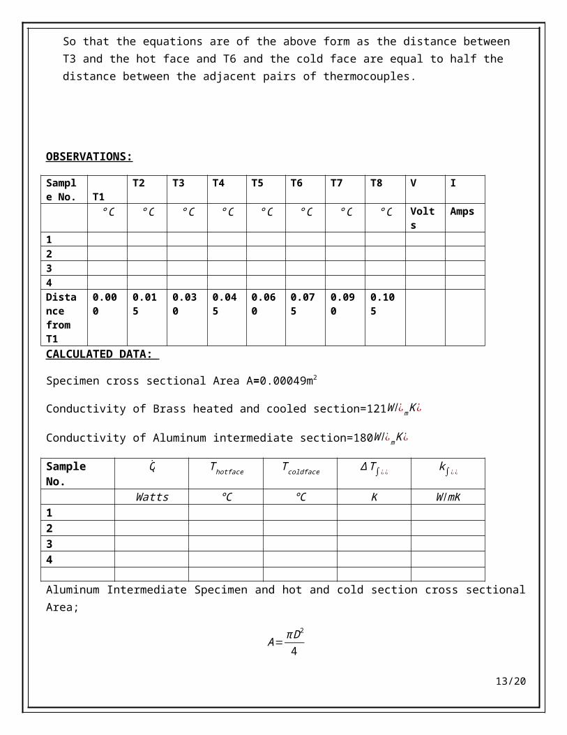
OBSERVATIONS:

Sample No.

T1 T2 T3 T4 T5 T6 T7 T8 V I

° C °C °C °C °C °C °C °C Volts Amps1234Distance from T1

0.000 0.015 0.030 0.045 0.060 0.075 0.090 0.105

CALCULATED DATA:

Brass Intermediate Specimen cross sectional Area A=0.00049m2

Sample No.

Q ∆ T1-3

hot

∆ T4-5

int

∆ T6-8

cold

∆x1-3

hot

∆x4-5

int

∆x6-8

cold

K1-3 K4-5 K6-8

Watts K K K m m m W /¿mK ¿W /¿mK ¿ W /¿mK ¿1234

The distance between the thermocouple sensors are as follows. Note that the distance between T4 and

T5 is less than the other pairs of thermocouples.

∆x1-3 = 0.03m

∆x4-5= 0.015m

∆x6-8= 0.03m

Heat transfer rate from the heater:

Q = V×I

Hence the thermal conductivity k of the section of bar are,

K1-3 = ∆ x1−3Q∆T 1−3 A

And similarly

K4-5 = ∆ x 4−5Q∆T 4−5 A

K6-8= ∆ x6−8Q∆T 6−8 A

5/20

It may be seen that the thermal conductivity in every case is similar. Difference occurs due to the heat losses from the specimen that is not accounted for.

GRAPH: Plot a graph b/w Temperature and Distance from T1 thermocouple.

COMMENTS:

6/20

EXPERIMENT # 02

OBJECTIVE:

To determine the thermal conductivity k of a metal specimen.

APPARATUS:


PROCEDURE:




4. Release the toggle clamp tensioning screw and clamps. Ensure that the faces of the exposed ends of the heated and cooled sections are clean. Similarly, check the faces of the Aluminum Intermediate specimen to be placed between the faces of the heated and cooled section. Coat the mating faces of the heated and cooled sections and the Aluminum intermediate section with thermal conduction paste. Ensure the intermediate section to be used is in the correct orientation then clamp the assembly together using the toggle clamps and tensioning screw.



7. Monitor temperatures T1, T2, T3, T4, T5, T6, T7, T8 until stable. When the temperatures are stabilized record:T1, T2, T3, T4, T5, T6, T7, T8, V, I

8. Increase the heater voltage by approximately 50 volts and repeat the above procedure again recording the parameters T1, T2, T3, T4, T5, T6, T7, T8, V, I when temperature have stabilized.




7/20


8/20

USEFUL DATA

Linear Heat Transfer Unit h111A

Heated Section:


Cooled Section:


Brass Intermediate Specimen:

Material: Brass 25 mm diameters * 30mm long. Thermocouples T4, T5 at 15mm spacing centrally spaced along the length. Thermal Conductivity: Approximately 121 W/mK

Stainless Steel Intermediate Specimen:

Material: Stainless Steel, 25 mm diameters * 30mm long. No Thermocouples fitted.


Aluminum Intermediate Specimen:

Material: Aluminum Alloy, 25 mm diameters * 30mm long. No Thermocouples fitted.


Reduced Diameter Brass Intermediate Specimen:

Material: Brass, 13 mm diameters * 30mm long. No Thermocouples fitted.


Hot and Cold Face Temperature:

Due to the need to keep the spacing of the thermocouples constant at 15mm with, or without the intermediate specimens in position the thermocouples are displaced 7.5 mm back from the ends faces of the heated and cooled specimens and similarly located for the Brass Intermediate Specimen.

T hot face = T3-(T 2−T 3)/2 T cold face = T6 + (T 6+T 7)/2

So that the equations are of the above form as the distance between T3 and the hot face and T6 and the cold face are equal to half the distance between the adjacent pairs of thermocouples.

9/20

OBSERVATIONS:

Sample No.

T1 T2 T3 T4 T5 T6 T7 T8 V I

° C °C °C °C °C °C °C °C Volts Amps1234Distance from T1

0.000 0.015 0.030 0.045 0.060 0.075 0.090 0.105

CALCULATED DATA:

Specimen cross sectional Area A=0.00049m2

Conductivity of Brass heated and cooled section=121W /¿mK ¿

Conductivity of Aluminum intermediate section=180W /¿mK ¿

Sample No. Q̇ T hotface T coldface ∆T∫¿ ¿k∫¿¿

Watts ℃ ℃ K W /mK1234

Aluminum Intermediate Specimen and hot and cold section cross sectional Area;

A=π D2

4

Heat transfer rate from the heater;

Q̇=V∗I

Note that the thermocouples T3 and T6 do not record the hot face and cold face temperatures, as are both displaced by 0.0075m from T3 and T6 as shown.

10/20

If it is assumed that the temperature distribution is linear, then the actual temperature at the hot face and cold face may be determined from the following equations.

T hotface=T 3−(T 2−T 3)2

And

T coldface=T 6+(T 6−T 7)

2

Hence

∆T ¿¿

From the above parameters, the thermal conductivity of the aluminum intermediate section may be calculated.

k∫¿=Q̇

∆ x∫ ¿

A∫ ¿(T hotface−T coldface)=Q̇

∆ x∫¿

A∫ ¿∆ T∫¿¿¿ ¿ ¿

¿¿

The thermal conductivity of the aluminum intermediate sample may also be calculated from the data it is plotted on a graph. This allows the T hotface and T coldface to be determined by extrapolating the time back from T3 and T6 to the hot face and cold face positions on the graph.

From the graph the slope of the line is ;

∆T∫¿

∆ x∫¿=¿¿

¿X

Hence

k∫¿= Q̇

A∗∆T∫¿

∆ x∫¿ ¿¿¿


COMMENTS:

11/20

EXPERIMENT # 03

OBJECTIVE:

To measure the temperature distribution for steady state conduction of energy through a composite plane wall and determine the overall Heat Transfer Coefficient for the flow of heat through a combination of different materials in use.

APPARATUS:


PROCEDURE:

1. Ensure that the main switch is in the off position (the digital displays should not be illuminated).

Ensure that the residual current circuit breaker on the rear panel is in the ON position.

2. Turn the voltage controller anti-clockwise to set the AC voltage to minimum.

3. Ensure the cold water supply and electrical supply is turned on at the source. Open the water tap

until the flow through the drain hose is approximately 1.5 liters/minute. The actual flow can be

checked using a measuring vessel and stopwatch if required but this is not a critical parameter. The

flow has to dissipate up to 65W only.

4. Release the toggle clamp tensioning screw and clamps. Ensure that the faces of the exposed ends

of the heated and cooled sections are clean. Similarly, check the faces of the the stainless steel

intermediate specimen to be placed between the faces of the heated and cooled section. Coat the

mating faces of the heated and cooled sections and the intermediate section with thermal

conduction paste. Ensure the intermediate section to be used is in the correct orientation then

clamp the assembly together using the toggle clamps and tensioning screw.

5. Turn on the main switch and the digital displays should illuminate. Set the temperature selector

switch to T1 to indicate the temperature of the heated end of the bar.

6. Following the above procedure ensure cooling water is flowing and then set the heater voltage V to

approximately 90 volts. This will provide a reasonable temperature gradient along the length of the

bar. If however the local cooling water supply is at a high temperature (25-35℃ or more) then it

may be necessary to increase the voltage supplied to the heater. This will increase the temperature

difference between the hot and cold ends of the bar.

7. Monitor temperatures T1, T2, T3, T6, T7, T8 until stable. When the temperatures are stabilized

record:T1, T2, T3, T6, T7, T8, V, I

8. Increase the heater voltage by approximately 50 volts and repeat the above procedure again

recording the parameters T1, T2, T3, T6, T7, T8, V, I when temperature have stabilized.

12/20

9. When the experimental procedure is completed, it is good practice to turn off the power to the

heater by reducing the voltage to zero and allow the system a short time to cool before turning off

the cooling water supply.

10. Ensure that the locally supplied water supply isolation valve to the unit is closed. Turn off the main

switch and isolate the electrical supply.

11. Note that if the thermal conducting paste is left on the mating faces of the heating and cooled

sections for a long period it can be more difficult to remove than if removed immediately after

completing an experiment. If left on the intermediate sections it can attract dust and in particular

grit which acts as a barrier to good thermal conduct.


13/20

OBSERVATIONS

Sample test result

Sample No. T1 T2 T3 T4 T5 T6 T7 T8 V I℃ ℃ ℃ ℃ ℃ ℃ ℃ ℃ Volts Amps

1234Distance from T1

0.000 0.015 0.030 0.045

0.060 0.075 0.090

0.105

CALCULATED DATA

Specimen cross sectional Area A = 0.00049m2

Conductivity of Brass heated and cooled section =121W /¿mK ¿

Conductivity of Stainless steel intermediate section =25W /¿mK ¿

Sample No.

Q ∆T 1−8 ∆ xhot ∆ x∫¿ ¿∆ xcold k hot k∫¿¿

k cold

-- W K m m m WmK

WmK

WmK

1234

Sample No. U= 1

( x hotk hot

+ xintkint

+ xcoldkcold

)

QA (T 1−T 8)

=U

-- Wm2K

Wm2K

1234

Brass Intermediate Specimen and hot and cold section cross sectional Area;

A=π D2

4

The temperature difference across the bar from T1 to T8;

14/20

T 1−T 8=¿X

Note that ∆ xhot and ∆ xcoldare the distances between the thermocouple T1 and the hot face and the cold face and the thermocouple T8 respectively. Similarly ∆ x∫¿ ¿ is the distance between the hot face and cold face of the intermediate stainless steel section.

The distances between surfaces are therefore as follows.

∆ xhot=¿ ¿ 0.0375m

∆ x∫¿ 0.030m

∆ xcold=¿ 0.0375m


Q=V X I

Hence

U=¿ Q

A (T 1−T 8)

15/20

Similarly

U= 1

( x hotk hot

+ xintkint

+ xcoldkcold

)

Note that the U value resulting from the test data differs from that resulting from assumed thermal conductivity and material thickness. This is most likely due to un-accounted for heat losses and thermal resistances between the hot face interface and cold face inter face with the stainless steel intermediate section.

The temperature data may be plotted against position along the bar and straight lines drawn through the temperature points for the heated and cooled sections. Then a straight line may be drawn through the hot face and cold face temperature to extrapolate the temperature distribution in the stainless steel intermediate section.


COMMENTS:

16/20

EXPERIMENT # 04

OBJECTIVE:

To measure the temperature distribution for steady state conduction of energy through a uniform plane wall and demonstrate the effect of a change in heat flow.

APPARATUS:


PROCEDURE:




4. Release the toggle clamp tensioning screw and clamps. Ensure that the faces of the exposed ends of the heated and cooled sections are clean. Coat the mating faces of the heated and cooled sections and with thermal conduction paste and clamp those together without any intermediate section in place.



7. Monitor temperatures T1, T2, T3, T6, T7, and T8 until stable. When the temperatures are stabilized record:T1, T2, T3, T6, T7, T8, V, I

8. Reset heater voltage to 120 volts and repeat the above procedure again and Monitor temperatures T1, T2, T3, T6, T7, T8 until stable. When the temperatures are stabilized record:T1, T2, T3, T6, T7, T8, V, I


17/20






OBSERVATIONS:

Sample test results

Sample No.

T1 T2 T3 T4 T5 T6 T7 T8 V I

℃ ℃ ℃ ℃ ℃ ℃ ℃ ℃ Volts Amps123

18/20

4Distance From TI

0.000 0.015 0.030 ----- ---- 0.045 0.060 0.075 ---- ----

CALCULATED DATA:

Sample No.

Q̇ ∆T 1-3

∆T 6-8

∆ x 1-3

∆ x 6-8

∆T 1−3

∆ x1−3

∆T 6−8

∆ x6−8Q̇ /(

∆T 1−3

∆ x1−3) Q̇ /(

∆T 6−8

∆ x6−8)

W ℃ ℃ m m ℃/m ℃/m W/mK W/mK1234


Q̇=V∗I

Temperature difference in the heated section between T1 and T3;

∆T hot=∆T1−3=T 1−T 3

Similarly the temperature difference in the cooled section between T6 and T8;

∆T cold=∆T6−8=T 6−T 8

The distance between the temperatures measuring points, T1 and T3and T6 and T8, are similar;

∆ x1−3=

∆ x6−8=

Hence the temperature gradient along the heated and cooled sections may be calculated from

Heated Section=∆T 1−3

∆x1−3=¿

Cooled Section=∆T6−8

∆x6−8=¿

If the constant rate of heat transfer is divided by the temperature gradients, the value obtained will be similar if the equation is valid.

Q̇=C ∆T∆x

19/20

Q̇

(∆T∆ x )=C

Hence, substituting the values obtained gives for the heated section and cooled sections respectively for following values.

Q̇

(∆T 1−3

∆ x1−3 )=¿¿

Q̇

(∆T 6−8

∆ x6−8 )=¿¿

As may be seen from the above example and the tabulated data the function does result in a constant value within the limits of the experimental data.

Q̇

(∆T∆ x )=C


COMMENTS:

20/20

Documents

engineersedge.weebly.comengineersedge.weebly.com/.../4680709/experiment1-4_hmt_.docx · Web viewStudent’s Version. HEAT & MASS FLOW PROCESSES. LINEAR HEAT TRANSFER UNIT H111A. EXPERIMENT