Embed Size (px)
Citation preview

OpenStat Reference Manual/Miller William G. Miller©2013
OpenStat Reference Manual
Second Edition
by
William G. Miller, PhD
November, 2015
1

OpenStat Reference Manual/Miller William G. Miller©2013
TABLE OF CONTENTS
Contents
OPENSTAT REFERENCE MANUAL......................................................................................................................... 1
TABLE OF CONTENTS........................................................................................................................................... 2
TABLE OF FIGURES.............................................................................................................................................. 6
PREFACE........................................................................................................................................................... 10
I. INTRODUCTION............................................................................................................................................ 11
II. INSTALLING OPENSTAT................................................................................................................................ 11
III. STARTING OPENSTAT.................................................................................................................................. 12
IV. FILES.......................................................................................................................................................... 13
CREATING A FILE............................................................................................................................................................13ENTERING DATA.............................................................................................................................................................15SAVING A FILE................................................................................................................................................................16HELP............................................................................................................................................................................17THE VARIABLES MENU....................................................................................................................................................17THE EDIT MENU.............................................................................................................................................................20THE ANALYSES MENU.....................................................................................................................................................25THE SIMULATION MENU..................................................................................................................................................25SOME COMMON ERRORS!................................................................................................................................................26
V. DISTRIBUTIONS.......................................................................................................................................... 28
USING THE DISTRIBUTION PARAMETER ESTIMATES PROCEDURE...............................................................................................28USING THE BREAKDOWN PROCEDURE.................................................................................................................................29USING THE DISTRIBUTION PLOTS AND CRITICAL VALUES PROCEDURE........................................................................................29
VI. DESCRIPTIVE ANALYSES.............................................................................................................................. 30
FREQUENCIES.................................................................................................................................................................30CROSS-TABULATION........................................................................................................................................................33BREAKDOWN.................................................................................................................................................................35DISTRIBUTION PARAMETERS.............................................................................................................................................37BOX PLOTS....................................................................................................................................................................37THREE VARIABLE ROTATION..............................................................................................................................................40X VERSUS Y PLOTS.........................................................................................................................................................41HISTOGRAM / PIE CHART OF GROUP FREQUENCIES...............................................................................................................43STEM AND LEAF PLOT......................................................................................................................................................45COMPARE OBSERVED AND THEORETICAL DISTRIBUTIONS........................................................................................................46QQ AND PP PLOTS.........................................................................................................................................................47NORMALITY TESTS..........................................................................................................................................................48RESISTANT LINE..............................................................................................................................................................50REPEATED MEASURES BUBBLE PLOT..................................................................................................................................52
2

OpenStat Reference Manual/Miller William G. Miller©2013
SMOOTH DATA BY AVERAGING.........................................................................................................................................54X VERSUS MULTIPLE Y PLOT.............................................................................................................................................56COMPARE OBSERVED TO A THEORETICAL DISTRIBUTION.........................................................................................................58MULTIPLE GROUPS X VERSUS Y PLOT.................................................................................................................................59
VII. CORRELATION........................................................................................................................................... 61
THE PRODUCT MOMENT CORRELATION..............................................................................................................................61TESTING HYPOTHESES FOR RELATIONSHIPS AMONG VARIABLES: CORRELATION..........................................................................62SIMPLE LINEAR REGRESSION.............................................................................................................................................63PARTIAL AND SEMI_PARTIAL CORRELATIONS........................................................................................................................66AUTOCORRELATION.........................................................................................................................................................68
VIII. COMPARISONS......................................................................................................................................... 75
ONE SAMPLE TESTS........................................................................................................................................................75PROPORTION DIFFERENCES...............................................................................................................................................77T-TESTS........................................................................................................................................................................79ONE, TWO OR THREE WAY ANALYSIS OF VARIANCE..............................................................................................................82A, B AND C FACTORS WITH B NESTED IN A.........................................................................................................................99LATIN AND GRECO-LATIN SQUARE DESIGNS.......................................................................................................................1022 OR 3 WAY FIXED ANOVA WITH 1 CASE PER CELL............................................................................................................129TWO WITHIN SUBJECTS ANOVA....................................................................................................................................132
IX. MULTIVARIATE PROCEDURES.................................................................................................................... 135
ANALYSIS OF VARIANCE USING MULTIPLE REGRESSION METHODS.........................................................................................135SUMS OF SQUARES BY REGRESSION..................................................................................................................................140THE GENERAL LINEAR MODEL.........................................................................................................................................144USING OPENSTAT TO OBTAIN CANONICAL CORRELATIONS...................................................................................................145BINARY LOGISTIC REGRESSION.........................................................................................................................................149COX PROPORTIONAL HAZARDS SURVIVAL REGRESSION........................................................................................................151WEIGHTED LEAST-SQUARES REGRESSION..........................................................................................................................1532-STAGE LEAST-SQUARES REGRESSION.............................................................................................................................159NON-LINEAR REGRESSION..............................................................................................................................................164
IX. MULTIVARIATE......................................................................................................................................... 168
DISCRIMINANT FUNCTION / MANOVA............................................................................................................................169CLUSTER ANALYSES.......................................................................................................................................................177PATH ANALYSIS............................................................................................................................................................187FACTOR ANALYSIS.........................................................................................................................................................196GENERAL LINEAR MODEL (SUMS OF SQUARES BY REGRESSION)............................................................................................202MEDIAN POLISH ANALYSIS.............................................................................................................................................211BARTLETT TEST OF SPHERICITY........................................................................................................................................212CORRESPONDENCE ANALYSIS..........................................................................................................................................214LOG LINEAR SCREENING, AXB AND AXBXC ANALYSES.........................................................................................................218
X. NON-PARAMETRIC..................................................................................................................................... 240
CONTINGENCY CHI-SQUARE............................................................................................................................................240SPEARMAN RANK CORRELATION......................................................................................................................................242MANN-WHITNEY U TEST...............................................................................................................................................243FISHER’S EXACT TEST....................................................................................................................................................245KENDALL’S COEFFICIENT OF CONCORDANCE.......................................................................................................................246KRUSKAL-WALLIS ONE-WAY ANOVA..............................................................................................................................247WILCOXON MATCHED-PAIRS SIGNED RANKS TEST..............................................................................................................249
3

OpenStat Reference Manual/Miller William G. Miller©2013
COCHRAN Q TEST.........................................................................................................................................................250SIGN TEST...................................................................................................................................................................251FRIEDMAN TWO WAY ANOVA......................................................................................................................................252PROBABILITY OF A BINOMIAL EVENT.................................................................................................................................254RUNS TEST..................................................................................................................................................................255KENDALL'S TAU AND PARTIAL TAU...................................................................................................................................257KAPLAN-MEIER SURVIVAL TEST.......................................................................................................................................259THE KOLMOGOROV-SMIRNOV TEST.................................................................................................................................266
XI. MEASUREMENT.......................................................................................................................................... 270
ANALYSIS OF VARIANCE: TREATMENT BY SUBJECT AND HOYT RELIABILITY................................................................................276KUDER-RICHARDSON #21 RELIABILITY..............................................................................................................................278WEIGHTED COMPOSITE TEST RELIABLITY...........................................................................................................................279RASCH ONE PARAMETER ITEM ANALYSIS..........................................................................................................................280GUTTMAN SCALOGRAM ANALYSIS....................................................................................................................................284SUCCESSIVE INTERVAL SCALING.......................................................................................................................................285DIFFERENTIAL ITEM FUNCTIONING...................................................................................................................................287ADJUSTMENT OF RELIABILITY FOR VARIANCE CHANGE.........................................................................................................302POLYTOMOUS DIF ANALYSIS...........................................................................................................................................305GENERATE TEST DATA...................................................................................................................................................309SPEARMAN-BROWN RELIABILITY PROPHECY.......................................................................................................................312
XII. STATISTICAL PROCESS CONTROL..............................................................................................................313
XBAR CHART..............................................................................................................................................................313RANGE CHART.............................................................................................................................................................316S CONTROL CHART.......................................................................................................................................................318CUSUM CHART...........................................................................................................................................................321P CHART.....................................................................................................................................................................323DEFECT (NON-CONFORMITY) C CHART..............................................................................................................................325DEFECTS PER UNIT U CHART...........................................................................................................................................327
XIII LINEAR PROGRAMMING....................................................................................................................... 329
THE LINEAR PROGRAMMING PROCEDURE..........................................................................................................................329
XIV USING MATMAN....................................................................................................................................... 333
PURPOSE OF MATMAN.................................................................................................................................................333USING MATMAN.........................................................................................................................................................333USING THE COMBINATION BOXES....................................................................................................................................334FILES LOADED AT THE START OF MATMAN........................................................................................................................334CLICKING THE MATRIX LIST ITEMS....................................................................................................................................334CLICKING THE VECTOR LIST ITEMS....................................................................................................................................334CLICKING THE SCALAR LIST ITEMS....................................................................................................................................334THE GRIDS..................................................................................................................................................................334OPERATIONS AND OPERANDS..........................................................................................................................................335MENUS.......................................................................................................................................................................335COMBO BOXES.............................................................................................................................................................335THE OPERATIONS SCRIPT...............................................................................................................................................335GETTING HELP ON A TOPIC.............................................................................................................................................336SCRIPTS......................................................................................................................................................................336FILES..........................................................................................................................................................................338ENTERING GRID DATA...................................................................................................................................................341MATRIX OPERATIONS....................................................................................................................................................343
4

OpenStat Reference Manual/Miller William G. Miller©2013
VECTOR OPERATIONS....................................................................................................................................................349SCALAR OPERATIONS.....................................................................................................................................................351
XV THE GRADEBOOK PROGRAM...................................................................................................................... 352
THE GRADEBOOK MAIN FORM.......................................................................................................................................352THE STUDENT PAGE TAB................................................................................................................................................353TEST RESULT PAGE TABS................................................................................................................................................354
XVI THE ITEM BANKING PROGRAM.............................................................................................................356
INTRODUCTION.............................................................................................................................................................356ITEM CODING..............................................................................................................................................................356USING THE ITEM BANK PROGRAM...................................................................................................................................358SPECIFYING A TEST........................................................................................................................................................358
BIBLIOGRAPHY................................................................................................................................................ 361
INDEX............................................................................................................................................................. 366
5

OpenStat Reference Manual/Miller William G. Miller©2013
TABLE OF FIGURESFigure 3.1 OpenStat Main Form..................................................................................................................................12Figure 4.1 The Variables Definition Form..................................................................................................................14Figure 4.2 The Options Form.......................................................................................................................................15Figure 4.3 The Form for Saving a File........................................................................................................................16Figure 4.4 The Variable Transformation Form............................................................................................................18Figure 4.5 The Variables Equation Option..................................................................................................................19Figure 4.6 Result of Using the Equation Option..........................................................................................................20Figure 4.7 The Sort Form.............................................................................................................................................20Figure 4.8 The Select Cases Form...............................................................................................................................22Figure 4.9 The Select If Form......................................................................................................................................23Figure 4.10 Random Selection of Cases Form............................................................................................................23Figure 4.11 Selection of a Range of Cases..................................................................................................................24Figure 4.12 The Recode Form.....................................................................................................................................24Figure 4.13 Selection of An Analysis from the Main Menu........................................................................................25Figure 5.1 Central Tendency and Variability Estimates..............................................................................................28Figure 6.1 Frequency Analysis Form...........................................................................................................................30Figure 6.2 Frequency Interval Form............................................................................................................................31Figure 6.3 Frequency Distribution Plot.......................................................................................................................33Figure 6.4 Cross-Tabulation Dialog Form....................................................................................................................34Figure 6.5 The Breakdown Form..................................................................................................................................35Figure 6.6 The Box Plot Form......................................................................................................................................38Figure 6.7 Box and Whiskers Plot................................................................................................................................40Figure 6.8 Three Dimension Plot with Rotation...........................................................................................................41Figure 6.9 X Versus Y Plot Form................................................................................................................................42Figure 6.10 Plot of Regression Line in X Versus Y.....................................................................................................43Figure 6.11 Form for a Pie Chart..................................................................................................................................44Figure 6.12 Pie Chart....................................................................................................................................................44Figure 6.13 Stem and Leaf Form..................................................................................................................................45Figure 6.14 Dialog Form for Examining Theoretical and Observed Distributions......................................................46Figure 6.15 The QQ / PP Plot Specification Form.......................................................................................................47Figure 6.16 A QQ Plot..................................................................................................................................................48Figure 6.17 Normality Tests.........................................................................................................................................49Figure 6.18 Resistant Line Dialog................................................................................................................................50Figure 6.19 Resistant Line Plot.....................................................................................................................................51Figure 6.20 Dialog for the Repeated Measures Bubble Plot........................................................................................52Figure 6.21 Bubble Plot................................................................................................................................................52Figure 6.22 Dialog for Smoothing Data by Averaging.................................................................................................54Figure 6.23 Smoothed Data Frequency Distribution Plot.............................................................................................54Figure 6.24 Cumulative Frequency of Smoothed Data................................................................................................55Figure 6.25 Dialog for an X Versus Multiple Y Plot....................................................................................................56Figure 6.26 X Versus Multiple Y Plot..........................................................................................................................57Figure 6.27 Dialog for Comparing Observed and Theoretical Distributions...............................................................58Figure 6.28 Comparison of an Observed and Theoretical Distribution........................................................................58Figure 6.29 Dialog for Multiple Groups X Versus Y Plot............................................................................................59Figure 6.30 X Versus Y Plot for Multiple Groups........................................................................................................60Figure 7.1 Correlation Regression Line........................................................................................................................62Figure 7.2 Simulated Bivariate Scatterplot...................................................................................................................63Figure 7.3 Single Sample Tests Form for Correlations................................................................................................63Figure 7.4 Comparison of Two Independent Correlations...........................................................................................64Figure 7.5 Comparison of Correlations for Dependent Samples..................................................................................65Figure 7.6 Form for Calculating Partial and Semi-Partial Correlations......................................................................66Figure 7.7 The Autocorrelation Form..........................................................................................................................68
6

OpenStat Reference Manual/Miller William G. Miller©2013
Figure 7.8 Moving Average Form...............................................................................................................................69Figure 7.9 Smoothed Plot Using Moving Average.......................................................................................................69Figure 7.10 Plot of Residuals Obtained Using Moving Averages...............................................................................70Figure 7.11 Polynomial Regression Smoothing Form.................................................................................................70Figure 7.12 Plot of Polynomial Smoothed Points........................................................................................................71Figure 7.13 Plot of Residuals from Polynomial Smoothing........................................................................................71Figure 7.14 Auto and Partial Autocorrelation Plot......................................................................................................74Figure 8.1 Single Sample Tests Dialog Form..............................................................................................................75Figure 8.2 Single Sample Proportion Test...................................................................................................................76Figure 8.3 Single Sample Variance Test......................................................................................................................77Figure 8.4 Test of Equality of Two Proportions..........................................................................................................78Figure 8.5 Test of Equality of Two Proportions Form................................................................................................79Figure 8.6 Comparison of Two Sample Means Form..................................................................................................80Figure 8.7 Comparison of Two Sample Means............................................................................................................80Figure 8.8 One, Two or Three Way ANOVA Dialog..................................................................................................82Figure 8.9 Plot of Sample Means From a One-Way ANOVA.....................................................................................83Figure 8.10 Specifications for a Two-Way ANOVA..................................................................................................84Figure 8.11 Within Subjects ANOVA Dialog.............................................................................................................86Figure 8.12 Treatment by Subjects ANOVA Dialog..................................................................................................88Figure 8.13 Plot of Treatment by Subjects ANOVA Means........................................................................................90Figure 8.14 Dialog for the Two-Way Repeated Measures ANOVA...........................................................................92Figure 8.15 Plot of Factor A Means in the Two-Way Repeated Measures Analysis..................................................93Figure 8.16 Plot of Factor B in the Two-Way Repeated Measures Analysis..............................................................94Figure 8.17 Plot of Factor A and Factor B Interaction in the Two-Way Repeated Measures Analysis......................95Figure 8.18 The Nested ANOVA Dialog....................................................................................................................97Figure 8.19 Three Factor Nested ANOVA Dialog......................................................................................................99Figure 8.20 Latin and Greco-Latin Squares Dialog...................................................................................................102Figure 8.21 Latin Squares Analysis Dialog...............................................................................................................103Figure 8.22 Four Factor Latin Square Design Dialog................................................................................................105Figure 8.23 Another Latin Square Specification Form..............................................................................................108Figure 8.24 Latin Square Design Form......................................................................................................................111Figure 8.25 Latin Square Plan 5 Specifications Form...............................................................................................114Figure 8.26 Latin Square Plan 6 Specification..........................................................................................................117Figure 8.27 Latin Squares Repeated Analysis Plan 7 Form......................................................................................120Figure 8.28 Latin Squares Repeated Analysis Plan 9 Form.....................................................................................123Figure 8.29 Dialog for 2 or 3 Way ANOVA with One Case Per Cell.......................................................................129Figure 8.30 One Case ANOVA Plot for Factor 1......................................................................................................130Figure 8.31 Factor 2 Plot for One Case ANOVA......................................................................................................131Figure 8.32 Interaction Plot of Two Factors for One Case ANOVA........................................................................131Figure 8.33 Dialog for Two Within Subjects ANOVA.............................................................................................132Figure 8.34 Factor One Plot for Two Within Subjects ANOVA..............................................................................133Figure 8.35 Factor Two Plot for Two Within Subjects ANOVA..............................................................................133Figure 8.36 Two Way Interaction for Two Within Subjects ANOVA......................................................................134Figure 9.1 Analysis of Covariance Dialog.................................................................................................................135Figure 9.2 Sum of Squares by Regression.................................................................................................................140Figure 9.3 Example 2 of Sum of Squares by Regression..........................................................................................142Figure 9.4 Canonical Correlation Analysis Form......................................................................................................145Figure 9.5 Logistic Regression Form.........................................................................................................................149Figure 9.6 Cox Proportional Hazards Survival Regression Form.............................................................................151Figure 9.7 Weighted Least Squares Regression........................................................................................................153Figure 9.8 Plot of Ordinary Least Squares Regression..............................................................................................156Figure 9.9 Plot of Weighted Least Squares Regression.............................................................................................158Figure 9.10 Two Stage Least Squares Regression Form...........................................................................................159Figure 9.11 Non-Linear Regression Specifications Form.........................................................................................164Figure 9.12 Scores Predicted by Non-Linear Regression Versus Observed Scores..................................................165
7

OpenStat Reference Manual/Miller William G. Miller©2013
Figure 9.13 Correlation Plot Between Scores Predicted by Non-Linear Regression and Observed Scores.............167Figure 111. Completed Non-Linear Regession Parameter Estimates of Regression Coefficients............................168Figure 9.14 Completed Non-Linear Regression Parameter Estimates of Regression Coefficients...........................168Figure 9.15 Specifications for a Discriminant Function Analysis.............................................................................169Figure 9.16 Plot of Cases in the Discriminant Space.................................................................................................176Figure 9.17 Hierarchical Cluster Analysis Form.......................................................................................................177Figure 9.18 Plot of Grouping Errors in the Discriminant Analysis...........................................................................182Figure 9.19 The K Means Clustering Form...............................................................................................................183Figure 9.20 Average Linkage Dialog Form...............................................................................................................184Figure 9.21 Path Analysis Dialog Form....................................................................................................................187Figure 9.22 Factor Analysis Dialog Form.................................................................................................................196Figure 9.23 Scree Plot of Eigenvalues.......................................................................................................................197Figure 9.24 The GLM Dialog Form..........................................................................................................................203Figure 9.25 GLM Specifications for a Repeated Measures ANOVA.......................................................................207Figure 9.26 A x B x R ANOVA Dialog Form...........................................................................................................209Figure 9.27 Dialog for the Median Polish Analysis..................................................................................................211Figure 9.28 Dialog for the Bartlett Test of Sphericity...............................................................................................212Figure 9.29 Dialog for Correspondence Analysis......................................................................................................214Figure 9.30 Correspondence Analysis Plot 1.............................................................................................................216Figure 9.31 Correspondence Analysis Plot 2.............................................................................................................217Figure 9.32 Correspondence Analysis Plot 3.............................................................................................................217Figure 9.33 Dialog for Log Linear Screening............................................................................................................218Figure 9.34 Dialog for the A x B Log Linear Analysis.............................................................................................220Figure 9.35 Dialog for the A x B x C Log Linear Analysis.......................................................................................223Figure 10.1 Contingency Chi-Square Dialog Form...................................................................................................240Figure 10.2 The Spearman Rank Correlation Dialog................................................................................................242Figure 10.3 The Mann=Whitney U Test Dialog Form..............................................................................................243Figure 10.4 Fisher's Exact Test Dialog Form............................................................................................................245Figure 10.5 Kendal's Coefficient of Concordance.....................................................................................................246Figure 10.6 Kruskal-Wallis One Way ANOVA on Ranks Dialog............................................................................247Figure 10.7 Wilcoxon Matched Pairs Signed Ranks Test Dialog.............................................................................249Figure 10.8 Cochran Q Test Dialog Form.................................................................................................................250Figure 10.9 The Matched Pairs Sign Test Dialog......................................................................................................251Figure 10.10 The Friedman Two-Way ANOVA Dialog...........................................................................................252Figure 10.11 The Binomial Probability Dialog.........................................................................................................254Figure 10.12 A Sample File for the Runs Test..........................................................................................................255Figure 10.13 The Runs Dialog Form.........................................................................................................................256Figure 10.14 Kendal's Tau and Partial Tau Dialog....................................................................................................257Figure 10.15 The Kaplan-Meier Dialog.....................................................................................................................261Figure 10.16 Experimental and Control Curves.......................................................................................................265Figure 10.17 A Sample File for the Kolmogorov-Smirnov Test...............................................................................266Figure 10.18 Dialog for the Kolmogorov-Smirnov Test...........................................................................................267Figure 10.19 Frequency Distribution Plot for the Kolmogorov-Smirnov Test.........................................................268Figure 11.1 Classical Item Analysis Dialog..............................................................................................................271Figure 11.2 Distribution of Test Scores (Classical Analysis)....................................................................................274Figure 11.3 Item Means Plot......................................................................................................................................275Figure 11.4 Hoyt Reliability by ANOVA.................................................................................................................276Figure 11.5 Within Subjects ANOVA Plot................................................................................................................277Figure 11.6 Kuder-Richardson Formula 20 Reliability Form...................................................................................278Figure 11.7 Composite Test Reliability Dialog.........................................................................................................279Figure 11.8 The Rasch Item Analysis Dialog............................................................................................................280Figure 11.9 Rasch Item Log Difficulty Estimate Plot...............................................................................................281Figure 11.10 Rasch Log Score Estimates..................................................................................................................281Figure 11.11 A Rasch Item Characteristic Curve......................................................................................................282Figure 11.12 A Rasch Test Information Curve..........................................................................................................282
8

OpenStat Reference Manual/Miller William G. Miller©2013
Figure 11.13 Guttman Scalogram Analysis Dialog...................................................................................................284Figure 11.14 Successive Interval Scaling Dialog......................................................................................................286Figure 11.15 Differential Item Functioning Dialog...................................................................................................288Figure 11.16 Differential Item Function Curves........................................................................................................297Figure 11.17 Another ItemDifferential Functioning Curve.......................................................................................297Figure 11.18 Reliability Adjustment for Variability Dialog......................................................................................304Figure 11.19 Polytomous Item Differential Functioning Dialog...............................................................................305Figure 11.20 Level Means for Polytomous Item.......................................................................................................307Figure 11.21 The Item Generation Dialog.................................................................................................................309Figure 11.22 Generated Item Data in the Main Grid.................................................................................................309Figure 11.23 Plot of Generated Test Data.................................................................................................................310Figure 11.24 Test of Normality for Generated Data..................................................................................................311Figure 11.25 Spearman-Brown Prophecy Dialog......................................................................................................312Figure 12.1 XBAR Chart Dialog...............................................................................................................................313Figure 12.2 XBAR Chart for Boltsize.......................................................................................................................315Figure 12.3 XBAR Chart Plot with Target Specifications........................................................................................316Figure 12.4 Range Chart Dialog................................................................................................................................317Figure 12.5 Range Chart Plot.....................................................................................................................................318Figure 12.6 Sigma Chart Dialog................................................................................................................................319Figure 12.7 Sigma Chart Plot.....................................................................................................................................320Figure 12.8 CUMSUM Chart Dialog.........................................................................................................................321Figure 12.9 CUMSUM Chart Plot.............................................................................................................................322Figure 12.10 p Control Chart Dialog.........................................................................................................................323Figure 12.11 p Control Chart Plot..............................................................................................................................324Figure 12.12 Defect c Chart Dialog...........................................................................................................................325Figure 12.13 Defect Control Chart Plot.....................................................................................................................326Figure 12.14 Defects U Chart Dialog........................................................................................................................327Figure 12.15 Defect Control Chart Plot.....................................................................................................................328Figure 13.1 Linear Programming Dialog...................................................................................................................329Figure 13.2 Example Specifications for a Linear Programming Problem.................................................................331Figure 14.1 The MatMan Dialog...............................................................................................................................333Figure 14.2 Using the MatMan Files Menu...............................................................................................................339Figure 15.1 The GradeBook Dialog...........................................................................................................................352Figure 15.2 The GradeBook Summary......................................................................................................................354Figure 15.3 The GradeBook Measurement Specifications Form..............................................................................355Figure 16.1 The Item Bank Form.............................................................................................................................358Figure 16.2 The Item Banking Test Specification Form...........................................................................................359Generate a Test...........................................................................................................................................................359Figure 16.3 The Form to Generate a Test..................................................................................................................359Figure 16.4 Student Verification Form for a Test Administration............................................................................360Figure 16.5 A Test Displayed on the Computer........................................................................................................360
9

OpenStat Reference Manual/Miller William G. Miller©2013
Preface
To the hundreds of graduate students and users of my statistics programs. Your encouragement, suggestions and patience have kept me motivated to maintain my interest in statistics and measurement.
To my wife who has endured my hours of time on the computer and wonders why I would want to create free material.
10

OpenStat Reference Manual/Miller William G. Miller©2013
I. Introduction
OpenStat, among others, are ongoing projects that I have created for use by students, teachers, researchers, practitioners and others. The software is a result of an “over-active” hobby of a retired professor (Iowa State University.) I make no claim or warranty as to the accuracy, completeness, reliability or other characteristics desirable in commercial packages (as if they can meet these requirement also.) They are designed to provide a means for analysis by individuals with very limited financial resources. The typical user is a student in a required social science or education course in beginning or intermediate statistics, measurement, psychology, etc. Some users may be individuals in developing nations that have very limited resources for purchase of commercial products.
Because I do not warrant them in any manner, you should insure yourself that the routines you use are adequate for your purposes. I strongly suggest analyses of text book examples and comparisons to other statistical packages where available. You should also be aware that I revise the program from time to time, correcting and updating OpenStat. For that reason, some of the images and descriptions in this book may not be exactly as you see when you execute the program. I update this book from time to time to try and keep the program and text coordinated.
II. Installing OpenStat
OpenStat has been successfully installed on Windows 95, 98, ME, XT, NT, VISTA ,Windows 7 and Windows 8 and Windows 10 systems. A free setup package (INNO) has been used to distribute and install OpenStat. Included in the setup file (OpenStatSetup.exe) is the executable file and Windows Help files (except Windows 10 charges extra for a .hlp file reader.) Sample data files that can be used to test the analysis programs are also available. Several Linux system users have also found that the free WINE software will allow OpenStat to run on a Linux platform.
To install OpenStat for Windows, follow these steps:
1. Connect to the internet address: http://statpages.info/miller
2. Click the download link for the OpenStatSetup.exe file
3. After the file has been downloaded, double click that program to initiate the installation of OpenStat. At the same website in 1 above, you will also find a link to a zip file containing sample data files that are useful for acquainting yourself with OpenStat. In addition, there are multiple tutorial files in Windows Media Video (.WMV) format as well as Power Point slide presentations.
11

OpenStat Reference Manual/Miller William G. Miller©2013
III. Starting OpenStat
To begin using a Windows version of OpenStat simply click the Windows “Start” button in the lower left portion of your screen, move the cursor to the “Programs” menu and click on the OpenStat entry. The following form should appear:
Figure 3.1 OpenStat Main Form
The above form contains several important areas. The “grid” is where data values are entered. Each column represents a “variable” and each row represents an “observation” or case. A default label is given for the first variable and each case of data you enter will have a case number. At the top of this “main” form there is a series of “drop-down” menu items. When you click on one of these, a series of options (and sometimes sub-options) that you can click to select. Before you begin to enter case values, you probably should “define” each variable to be entered in the data grid. Select the “VARIABLES” menu item and click the “Define” option. More will be said about this in the following pages.
12

OpenStat Reference Manual/Miller William G. Miller©2013
IV. Files
The “heart” of OpenStat or any other statistics package is the data file to be created, saved, retrieved and analyzed. Unfortunately, there is no one “best” way to store data and each data analysis package has its own method for storing data. Many packages do, however, provide options for importing and exporting files in a variety of formats. For example, with Microsoft’s Excel package, you can save a file as a file of “tab” separated fields. Other program packages such as SPSS can import “tab” files. Here are the types of file formats supported by OpenStat:
1. OPENSTAT binary files (with the file extension of .BIN .)2. Tab separated field files (with the file extension of .TAB.)3. Comma separated field files (with the file extension of .CSV.)4. Space separated field files (with the file extension of .SSV.)5. Text files (with the extension .TEX) NOTE: the file format in this text file is unique to OpenStat!6. Epidata files (this is a format used by Epidemiologists)7. Matrix files previously saved by OpenStat8. Fixed Format files in which the user specifies the record format
My preference is to save files as .TEX files. Alternatively, tab separated field files are often used. This gives you the opportunity to analyze the same data using a variety of packages. For relatively small files (say, for example, a file with 20 variables and 1000 cases), the speed of loading the different formats is similar and quite adequate. The default for OPENSTAT is to save as a binary file with the extension .TEX to differentiate it from other types of files.
Creating a File
When OPENSTAT begins, you will see a “grid” of two rows and two columns. The left-most column will automatically contain the word “Case” followed by a number (1 for the first case.) The top row will contain the names of the variables that you assign when you start entering data for the first variable. If you click your mouse on the “Variables” menu item, a drop-down list will appear that contains the word “define”. If you click on this label, the following form appears:
13

OpenStat Reference Manual/Miller William G. Miller©2013
Figure 4.1 The Variables Definition Form
In the above figure you will notice that a variable name has automatically been generated for the first variable. To change the default name, click the box with the default name and enter the variable name that you desire. It is suggested that you keep the length of the name to eight characters or less. Do NOT have any blanks in the variable name. An underscore (_) character may be used. You may also enter a long label for the variable. If you save your file as an OPENSTAT file, this long name (as well as other descriptive information) will be saved in the file (the use of the long label has not yet been implemented for printing output but may be in future versions.) To proceed, simply click the Return button in the lower right of this form. The default type of variable is a “floating point” value, that is, a number which may contain a decimal fraction. If a data field (grid cell) is left blank, the program will usually assume a missing value for the data. The default format of a data value is eight positions with two positions allocated to fractional decimal values (format 8.2.) By clicking on any of the specification fields you can modify these defaults to your own preferences. You can change the width of your field, the number of decimal places (0 for integers.) Another way to specify the default format and missing values is by modifying the "Options" file. When you click on the Options menu item and select the change options, the following form appears:
14

OpenStat Reference Manual/Miller William G. Miller©2013
Figure 4.2 The Options Form
In the options form you can specify the Data Entry Defaults as well as whether you will be using American or European formatting of your data (American's use a period (.) and Europeans use a comma (,) to separate the integer portion of a number from its fractional part.) The Printer Spacing section is currently ignored but may be implemented in a future version of OpenStat. You can also specify the directory in which to find the data files you want to process. I recommend that you save data in the same directory that contains the OpenStat program (the default directory.)
Entering Data
When you enter data in the grid of the main form there are several ways to navigate from cell to cell. You can, of course, simply click on the cell where you wish to enter data and type the data values. If you press the
15

OpenStat Reference Manual/Miller William G. Miller©2013
“enter” key following the typing of a value, the program will automatically move you to the next cell to the right of the current one or down to the next cell if you are at the last variable. You may also press the keyboard “down” arrow to move to the cell below the current one. If it is a new row for the grid, a new row will automatically be added and the “Case” label added to the first column. You may use the arrow keys to navigate left, right, up and down. You may also press the “Page Up” button to move up a screen at a time, the “Home” button to move to the beginning of a row, etc. Try the various keys to learn how they behave. You may click on the main form’s Edit menu and use the delete column or delete row options. Be sure the cursor is sitting in a cell of the row or column you wish to delete when you use this method. A common problem for the beginner is pressing the "enter" key when in the last column of their variables. If you do accidentally add a case or variable you do not wish to have in your file, use the edit menu and delete the unused row or variable. If you have made a mistake in the entry of a cell value, you can change it in the “Cell Edit” box just below the menu. In this box you can use the delete key, backspace key, enter characters, etc. to make the corrections for a cell value. When you press your “Enter” key, the new value will be placed in the corresponding cell. Notice that as you make grid entries and move to another cell, the previous value is automatically formatted according to the definition for that variable. If you try to enter an alphabetic character in an integer or floating point variable, you will get an error message when you move from that cell. To correct the error, click on the cell that is incorrect and make the changes needed in the Cell Edit box.
Saving a File
Once you have entered a number of values in the grid, it is a good idea to save your work (power outages do occur!) Go to the main form’s File menu and click it. You will see there are several ways to save your data. The first time you save your data you should click the “Save a Text Type of File” option. A “dialog box” will then appear as shown below:
Figure 4.3 The Form for Saving a File
Simply type the name of the file you wish to create in the File name box and click the Save button. After this initial save as operation, you may continue to enter data and save with the Save button on the file menu. Before you exit the program, be sure to save your file if you have made additions to it.
If you do not need to save specifications other than the short name of each variable, you may prefer to “export” the file in a format compatible to other programs. The “Export Tab File option under the File menu will save your data in a text file in which the cell values in each row are separated by a tab key character. A file with the extension .TAB will be created. The list of variables from the first row of the grid are saved first, then the first row of the data, etc. until all grid rows have been saved.
16

OpenStat Reference Manual/Miller William G. Miller©2013
Alternatively, you may export your data with a comma or a space separating the cell values. Basic language programs frequently read files in which values are separated by commas or spaces. If you are using the European format of fractional numbers, DO NOT USE the comma separated files format since commas will appear both for the fractions and the separation of values - clearly a design for disaster!
Help
Users of Microsoft Windows are used to having a “help” system available to them for instant assistance when using a program. Most of these systems provide the user the ability to press the “F1" key for assistance on a particular topic or by placing their cursor on a particular program item and pressing the right mouse button to get help. OpenStat for the Microsoft Windows does have a help file. Place the cursor on a menu topic and press the F1 key to see what happens! You can use the help system to learn more about OpenStat procedures. Again, as the program is revised, there may not yet be help topics for all procedures and some help topics may vary slightly from the actual procedure's operation. Vista and Windows 7 users may have to download a file from MicroSoft to provide the option for reading “.hlp” files.
The Variables Menu
Across the top of the "Main Form" is a series of "menu" items. Like the "File" menu, each of these menu items "drops-down" a series of options and these options may have sub-options. The "Variables" menu contains a variety of options to assist you in working with the variables (columns of data). These options include:1. Define2. Transform3. Print Dictionary4. Sort5. Create An Expanded File from a Frequencies File6. Enter an Equation to Combine Variables to Create a New Variable
The first option lets you enter or change a variable definition (see Figure 2 above.)
Another option lets you "transform" an existing variable to create a new variable. A variety of transformations are possible. If you elect this option, you will see the following dialogue form:
17

OpenStat Reference Manual/Miller William G. Miller©2013
Figure 4.4 The Variable Transformation Form
You will note that you can transform a variable by adding, subtracting, multiplying, dividing or raising a value to a power. To do this you select a variable to transform by clicking on the variable in the list of available variables and then clicking the right arrow. You then enter a constant by clicking on the box for the constant and entering a value. You select the transformation with a constant from among the first 10 possible transformations by clicking on the desired transformation (you will see it entered automatically in the lower right box.) Next you enter a name for the new variable in the box labeled "Save new variable as:" and click the OK button.
Sometimes you will want to transform a variable using one of the common exponentiation or trigonometric functions. In this case you do not need to enter a constant - just select the variable, the desired transformation and enter the variable name before clicking the OK button.
You can also select a transformation that involves two variables. For example, you may want a new variable that represents the sum, product, difference, etc. of two variables. In this case you select the two variables for the first and second arguments using the appropriate right-arrow key after clicking one and then the other in the available variables list.
The "Print Dictionary" option simply creates a list of variable definitions on an "output" form which may be printed on your printer for future reference.
The option to create a new variable by means of an equation can be useful in a variety of situations. For example, you may want to create a new variable that is simply the sum of several other variables (or products of, etc.) We have selected a file labeled “cansas.tab” from our sample files and will create a new variable labeled “physical” that adds the first three variables. When we click the equation option, the following form appears:
18

OpenStat Reference Manual/Miller William G. Miller©2013
Figure 4.5 The Variables Equation Option
To use the above, enter the name of your new variable in the box provided. Following this box are three additional “edit” boxes with “drop-down” boxes above each one. For the first variable to be added, click the drop-down box labeled “Variables” and select the name of your first variable. It will be automatically placed in the third box. Next, click the “Next Entry” button. Now click the “Operations” drop-down arrow and select the desired operation (plus in our example) and again select a variable from the Variables drop-down box. Again click the “Next Entry” button. Repeat the Operations and Variables for the last variable to be added. Click the “Finished” button to end the creation of the equation. Click the Compute button and then the Return button. An output of your equation will be shown first as below:
Equation Used for the New Variable
physical = weight + waist + pulse
You will see the new variable in the grid:
19

OpenStat Reference Manual/Miller William G. Miller©2013
Figure 4.6 Result of Using the Equation Option
The "Sort" option involves clicking on a cell in the column on which the cases are to be sorted and then selecting the Variables / Sort option. You then indicate whether you want to sort the cases in an ascending order or a descending order. The form below demonstrates the sort dialogue form:
Figure 4.7 The Sort Form
The Edit Menu
The Edit menu is provided primarily for deleting, cutting and pasting of cells, rows or columns of data. It also provides the ability to insert a new column or row at a desired position in the data grid. There is one special "paste" operation provided for users that also have the Microsoft Excel program and wish to copy cells from an Excel spreadsheet into the OpenStat grid. These operations involve clicking on a cell in a given row and column
20

OpenStat Reference Manual/Miller William G. Miller©2013
and the selecting the edit operation desired. The user is encourage to experiment with these operations in order to become familiar with them. The following options are available:1. Copy2. Delete3. Paste4. Insert a New Column5. Delete a Column6. Copy a Column7. Paste a Column8. Insert a New Row9. Delete a Row10. Copy a Row11. Paste a row12. Format Grid Values13. Select Cases14. Recode15. Switch USA to Euro or Vice Versa16. Swap Rows and Columns17. Open Output Form / Word Processor
The first eleven of these options involve copying, deleting, pasting a row, column or block of grid cells or inserting a new row or column. You can also “force” grid values to be reformatted by selecting option 12. This can be useful if you have changed the definition of a variable (floating point to integer, number of decimal places, etc.)In some cases you may need to swap the cell values in the rows and columns so that what was previously a row is now a column. If you receive files from an individual using a different standard than yourself, you can switch between European and USA standards for formatting decimal fraction values in the grid. Another useful option lets you “re-code” values in a selected variable. For example, you may need to recode values that are currently 0 to a 1 for all cases in your file.
The "Select Cases" option lets you analyze only those cases (rows) which you select. When you press this option you will see the following dialogue form:
21

OpenStat Reference Manual/Miller William G. Miller©2013
Figure 4.8 The Select Cases Form
Notice that you may select a random number of cases, cases the exhibit a specific range of values or cases if a specific condition exists. Once selection has been made, a new variable is added to the grid called the "Filter" variable. You can subsequently use this filter variable to delete uneeded cases from your file if desired. Each of the selection procedures invokes a dialogue form that is specific to the type of selection chosen. For example, if you select the "if condition is satisfied" button, you will see the following dialogue form:
22

OpenStat Reference Manual/Miller William G. Miller©2013
Figure 4.9 The Select If Form
An example has been entered on this form to demonstrate a typical selection criteria. Notice that compound statements involve the use of opening and closing parentheses around each expression You can directly enter values in the "if" box or use the buttons provided on the pad.
Should you select the "random" option in Figure 8 you would see the following form:
Figure 4.10 Random Selection of Cases Form
The user may select a percentage of cases or select a specific number from a specified number of cases.Finally, the user may select a specified range of cases. This option produces the following dialogue form:
23

OpenStat Reference Manual/Miller William G. Miller©2013
Figure 4.11 Selection of a Range of Cases
The Variables / Recode option is used to change the value of cases in a given variable. For example, you may have imported a file which originally coded gender as "M" or "F" but the analysis you want requires a coding of 0 and 1. You can select the recode option and get the following form to complete:
Figure 4.12 The Recode Form
Notice that you first click on the column of the variable to recode, enter the old value (or value range) and also enter the new value before clicking the Apply button. You can repeat the process for multiple old values before returning to the Main Form.
Some files may require the user to change all column values to row values and row values to column values. For example, a user may have created a file with rows that represent subjects measured on 10 variables. One of the desired analysis however requires the calculation of correlations among subjects, not variables. To obtain a matrix of this form the user can swap rows and columns. Clicking on this option will switch the rows and columns. In doing this, the original variable labels are lost. The previous cases are now labeled Var1, Var2, etc. and the original variables are labeled CASE 1, CASE 2, etc. Clearly, one should save the original file before completing this operation! Once the swap has occurred, you can save the new file under a different name.
The last option under the variables menu lets you switch between the American and European format for decimal fractions. This may be useful when you have imported a file from another country that uses the other format. OpenStat will attempt to convert commas to periods or vice-versa as required.
24

OpenStat Reference Manual/Miller William G. Miller©2013
The Analyses Menu
The heart of any statistics package is the ability to perform a variety of statistical analyses. Many of the typical analyses are included in the options and sub-options of the Analyses menu. The figure below shows the options and the sub-options under the descriptive option. No attempt will be made at this point in the text to describe each analysis - these are described further in the text.
Figure 4.13 Selection of An Analysis from the Main Menu
The Simulation Menu
As you read about and learn statistics, it is helpful to be able to simulate data for an analysis and see what the distribution of the values looks like. In addition, the concepts of "type I error", "type II error", "Power", correlation, etc. may be more readily grasped if the student can "play" with distributions and the effects of choices they might make in a real study. Under the simulation menu the user may generate a sequence of numbers, may generate multivariate data, may generate data that are a sample from a theoretical population or generate bivariate-normal data for a correlation. One can even generate data for a two-way analysis of variance!
Some Common Errors!
25

OpenStat Reference Manual/Miller William G. Miller©2013
Empty Cells
The beginning user will often see a message something like “” is not a valid floating point value. The most common cause of this error occurs when a procedure attempts to read a blank cell, that is, a cell that has been left empty by the user. The new user will typically use the down-arrow to move to the next row in the data grid in preparation to enter the next row of values. If you do this after entering the values for the last case, you will create a row of empty cells. You should put the cursor on one of these empty cells and use the Edit->Delete Row menu to remove this blank row.
The user should define the “Missing Value” for each variable when they define the variable. One should also click on the Options menu and place a missing value in that form. OpenStat attempts to place that missing value in empty cells when a file is saved as .TEX file. Not all OpenStat procedures allow missing values so you may have to delete cases with missing values for those procedures.
Incorrect Format for Floating Point Values
A second reason you might receive a “not valid” error is because you are using the European standard for the format of values with decimal fractions. Most of the statistical procedures contain a small “edit” window that contains a confidence level or a rejection area such as 95.0 or 0.05. These will NOT be valid floating point values in the European standard and the user will need to click on the value and replace it with the correct form such as 95,0 or 0,05. This has been done for the user in some procedures but not all!
String labels for Groups
Users of other statistics packages such as SPSS or Excel may have used strings of characters to identify different groups of cases (subjects or observations.) OpenStat uses sequential integer values only in statistical analyses such as analyses of variance or discriminant function analysis. An edit procedure has been included that permits the conversion of string labels to integer values and saves those integers in a new column of the data grid. An attempt to use a string (alphanumeric) value will cause an “not valid” type of error. Several procedures in OpenStat have been modified to let you specify a string label for a group variable and automatically create an integer value for the analysis in a few procedures but not all. It is best to do the conversion of string labels to integers and use the integer values as your group variable.
Floating Point Errors
Sometimes a procedure will report an error of the type “Floating Point Division Error”. This is often the outcome of a procedure attempting to divide a quantity by zero (0.) As an example, assume you have entered data for several variables obtained on a group of subjects. Also assume that the value observed for one of those variables is the same (a constant value) for all cases. In this situation there is no variability among the cases and the variance and standard deviation will be zero! Now an attempt to use that zero variance or standard deviation in the calculation of z scores, a correlation with another variable or other usage will cause an error (division by zero is not defined.)
Values too Large (or small)
In some fields of study such as astronomy the values observed may be very, very large. Computers use binary numbers to represent quantities. Nearly all OpenStat procedures use “double precision” storage for floating point values. The double precision value is stored in 64 binary “bits” in the computer memory. In most computers
26

OpenStat Reference Manual/Miller William G. Miller©2013
this is a combination of 8 binary “bytes” or words. The values are stored with a characteristic and mantissa similar to a scientific notation. Of course bits are also used to represent the sign of these parts. The maximum value for the characteristic is typically something like 2 raised to the power of 55 and the mantissa is 2 to the 7th power. Now consider a situation where you are summing the product of several of very large values such as is done in obtaining a variance or correlation. You may very well exceed the 64 bit storage of this large sum of products! This causes an “overflow” condition and a subsequent error message. The same thing can be said of values too small. This can cause an “underflow” error and associated error message.
The solution for these situations of values too large or too small is to “scale” your initial values. This is typically done by dividing or multiplying the original values by a constant to move the decimal point to decrease (or increase) the value. This does, of course, affect the “precision” of your original values but it may be a sacrifice necessary to do the analysis. In addition, the results will have to be “re-scaled” to reflect the original measurement scale.
27

OpenStat Reference Manual/Miller William G. Miller©2013
V. Distributions
Using the Distribution Parameter Estimates Procedure
One of the procedures which may be executed in your OpenStat package is the Analyses/Statistics/Central Tendency and Variability procedure. The procedure will compute the mean, variance, standard deviation, range, skew, minimum, maximum and number of cases for each variable you have specified. To use it, you enter your data as a column of numbers in the data grid or retrieve the data of a file into the data grid. Click on the Statistics option in the main menu and click on the Mean, Variance, Std.Dev, Skew, Kurtosis option under the Descriptive sub-menu. You will see the following form:
Figure 5.1 Central Tendency and Variability Estimates
Select the variables to analyze by clicking the variable name in the left column followed by clicking the right arrow. You may select ALL by clicking the All button. Click on the Continue button when you have selected all of your variables. Notice that you can also convert each of the variables to standardized z scores as an option. The new variables will be placed into the data grid with variable names created by combining z with the original variable names. The results will be placed in the output form which may be printed by clicking the Print button of that form.
Using the Breakdown Procedure
28

OpenStat Reference Manual/Miller William G. Miller©2013
The Breakdown procedure is an OpenStat program designed to produce the means and standard deviations of cases that have been classified by one or more other (categorical) variables. For example, a sample may contain subjects for which have values for interest in school, grade in school, gender, and rural/urban home environment. A researcher might be interested in reporting the mean and standard deviation of "interest in school" for persons classified by combinations of the other three (nominal scale) variables grade, gender and rural/urban.
The Breakdown program summarizes the means and standard deviations for each level of the variable entered last within levels of the next-to-last variable, etc. In our example, the statistics would be given for rural and urban codes within male and female levels first, then statistics for males and females within grade level and finally, the overall group means and standard deviations. The order of specification is therefore important. The variable receiving the finest breakdown is listed last, the next-most relevant breakdown next-to-last, etc. If the order of categorical variables for the above example were listed as 2, 4, 3 then the summary would give statistics for males and females within rural and urban codes, and rural and urban students (genders combined) within grade levels. Optionally, the user may request one-way analysis of variance results. An ANOVA table will be produced for the continuous variable for the categories of each of the nominal variables.
Using the Distribution Plots and Critical Values Procedure
This simulation procedure generates three possible distributions, i.e. (a) z scores, (b) Chi-squared statistics or (c) F ratio statistics. If you select either the Chi-squared or the F distribution, you will be asked to enter the appropriate degrees of freedom. You are also asked to enter the probability of a Type I error. The default value of 0.05 is commonly used. You may also elect to print the distribution that is created.
29

OpenStat Reference Manual/Miller William G. Miller©2013
VI. Descriptive Analyses
Frequencies
Selecting the Descritive/Distribution Frequencies option from the Analyses menu results in the following form being displayed. The cansas.TEX file has been loaded and the weight variable has been selected for analysis. The option to display a histogram has also been selected, the three dimensional vertical bars has been selected and the plotting of the normal distribution has been checked.
Figure 6.1 Frequency Analysis Form
When the OK button is clicked, each variable is analyzed in sequence. The first thing that is displayed is a form shown below:
Figure 6.2 Frequency Interval Form30

OpenStat Reference Manual/Miller William G. Miller©2013
You will notice that the number of intervals shown for the first variable (weight) is 16. You can change the interval size (and press return) to increase or decrease the number of intervals. If we change the interval size to 10 instead of the current 1, we would end up with 11 categories.
Now when the OK button on the specifications form is clicked the following results are displayed:
FREQUENCY ANALYSIS BY BILL MILLER
Frequency Analysis for waist FROM TO FREQ. PCNT CUM.FREQ. CUM.PCNT. %ILE RANK
31.00 32.00 1 0.05 1.00 0.05 0.03 32.00 33.00 1 0.05 2.00 0.10 0.07 33.00 34.00 4 0.20 6.00 0.30 0.20 34.00 35.00 3 0.15 9.00 0.45 0.38 35.00 36.00 2 0.10 11.00 0.55 0.50 36.00 37.00 3 0.15 14.00 0.70 0.63 37.00 38.00 3 0.15 17.00 0.85 0.78 38.00 39.00 2 0.10 19.00 0.95 0.90 39.00 40.00 0 0.00 19.00 0.95 0.95 40.00 41.00 0 0.00 19.00 0.95 0.95 41.00 42.00 0 0.00 19.00 0.95 0.95 42.00 43.00 0 0.00 19.00 0.95 0.95 43.00 44.00 0 0.00 19.00 0.95 0.95 44.00 45.00 0 0.00 19.00 0.95 0.95 45.00 46.00 0 0.00 19.00 0.95 0.95 46.00 47.00 1 0.05 20.00 1.00 0.97
The above results of the output form show the intervals, the frequency of scores in the intervals, the percent of scores in the intervals, the cumulative frequencies and percents and the percentile ranks. Clicking the Return button then results in the display of the frequencies expected under the normal curve for the data:
Interval ND Freq. 1 0.97 2 1.42 3 1.88 4 2.26 5 2.46 6 2.44 7 2.19 8 1.79 9 1.33 10 0.89 11 0.54 12 0.30 13 0.15 14 0.07 15 0.03 16 0.01 17 0.00
When the Return button is again pressed the histogram is produced as illustrated below:31

OpenStat Reference Manual/Miller William G. Miller©2013
Figure 6.3 Frequency Distribution Plot
Cross-Tabulation
A researcher may observe objects classified into categories on one or more nominal variables. It is desirable to obtain the frequencies of the cases within each “cell” of the classifications. An example is shown in the following description of using the cross-tabulation procedure. Select the cross-tabulation option from the Descriptive option of the Statistics menu. You see a form like that below:
32

OpenStat Reference Manual/Miller William G. Miller©2013
Figure 6.4 Cross-Tabulation Dialog Form
In this example we have opened the chisquare.tab file to analyze. Cases are classified by “row” and “col” variables. When we click the OK button we obtain:
CROSSTABULATION ANALYSIS PROGRAM
VARIABLE SEQUENCE FOR THE CROSSTABS:row (Variable 1) Lowest level = 1 Highest level = 3col (Variable 2) Lowest level = 1 Highest level = 4
FREQUENCIES BY LEVEL:For Cell Levels: row : 1 col: 1 Frequency = 5For Cell Levels: row : 1 col: 2 Frequency = 5For Cell Levels: row : 1 col: 3 Frequency = 5For Cell Levels: row : 1 col: 4 Frequency = 5Number of observations for Block 1 = 20For Cell Levels: row : 2 col: 1 Frequency = 10For Cell Levels: row : 2 col: 2 Frequency = 4For Cell Levels: row : 2 col: 3 Frequency = 7For Cell Levels: row : 2 col: 4 Frequency = 3Number of observations for Block 2 = 24For Cell Levels: row : 3 col: 1 Frequency = 5For Cell Levels: row : 3 col: 2 Frequency = 10For Cell Levels: row : 3 col: 3 Frequency = 10For Cell Levels: row : 3 col: 4 Frequency = 2Number of observations for Block 3 = 27Cell Frequencies by Levels
col 1 2 3 4 Block 1 5.000 5.000 5.000 5.000 Block 2 10.000 4.000 7.000 3.000 Block 3 5.000 10.000 10.000 2.000
Grand sum for all categories = 71
Note that the count of cases is reported for each column within rows 1, 2 and 3. If we had specified the col variable prior to the row variable, the procedure would summarize the count for each row within columns 1 through 4.
33

OpenStat Reference Manual/Miller William G. Miller©2013
Breakdown
If a researcher has observed a continuous variable along with classifications on one or more nominal variables, it may be desirable to obtain the means and standard deviations of cases within each classification combination. In addition, the researcher may be interested in testing the hypothesis that the means are equal in the population sampled for cases in the categories of each nominal variable. We will use sample data that was originally obtained for a three-way analysis of variance (threeway.tab.) We then select the Breakdown option from within the Descriptive option on the Statistics menu and see:
Figure 6.5 The Breakdown Form
We have elected to obtain a one-way analysis of variance for the means of cases classified into categories of the “Slice” variable for each level of the variable “Col.” and variable “Row”. When we click the Continue button we obtain the first part of the output which is:
BREAKDOWN ANALYSIS PROGRAM
VARIABLE SEQUENCE FOR THE BREAKDOWN:Row (Variable 1) Lowest level = 1 Highest level = 2Col. (Variable 2) Lowest level = 1 Highest level = 2Slice (Variable 3) Lowest level = 1 Highest level = 3
Variable levels: Row level = 1Col. level = 1Slice level = 1
Freq. Mean Std. Dev. 3 2.000 1.000
34

OpenStat Reference Manual/Miller William G. Miller©2013
Variable levels: Row level = 1Col. level = 1Slice level = 2
Freq. Mean Std. Dev. 3 3.000 1.000
Variable levels: Row level = 1Col. level = 1Slice level = 3
Freq. Mean Std. Dev. 3 4.000 1.000 Number of observations across levels = 9Mean across levels = 3.000Std. Dev. across levels = 1.225
We obtain similar output for each level of the “Col.” variable within each level of the “Row” variable as well as the summary across all rows and columns. The procedure then produces the one-way ANOVA’s for the breakdowns shown. For example, the first ANOVA table for the above sample is shown below:
Variable levels: Row level = 1Col. level = 2Slice level = 1
Freq. Mean Std. Dev. 3 5.000 1.000
Variable levels: Row level = 1Col. level = 2Slice level = 2
Freq. Mean Std. Dev. 3 4.000 1.000
Variable levels: Row level = 1Col. level = 2Slice level = 3
Freq. Mean Std. Dev. 3 3.000 1.000 Number of observations across levels = 9Mean across levels = 4.000Std. Dev. across levels = 1.225
ANALYSES OF VARIANCE SUMMARY TABLES
Variable levels:
35

OpenStat Reference Manual/Miller William G. Miller©2013
Row level = 1Col. level = 1Slice level = 1
Variable levels: Row level = 1Col. level = 1Slice level = 2
Variable levels: Row level = 1Col. level = 1Slice level = 3
SOURCE D.F. SS MS F Prob.>FGROUPS 2 6.00 3.00 3.000 0.3041WITHIN 6 6.00 1.00TOTAL 8 12.00
The last ANOVA table is:
ANOVA FOR ALL CELLS
SOURCE D.F. SS MS F Prob.>FGROUPS 11 110.75 10.07 10.068 0.0002WITHIN 24 24.00 1.00TOTAL 35 134.75FINISHED
You should note that the analyses of variance completed do NOT consider the interactions among the categorical variables. You may want to compare the results above with that obtained for a three-way analysis of variance completed by either the 1,2, or 3 way randomized design procedure or the Sum of Squares by Regression procedure listed under the Analyses of Variance option of the Statistics menu.
Distribution Parameters
The distribution parameters procedure was previously described.
Box Plots
Box plots are useful graphical devices for viewing both the central tendency and the variability of a continuous variable. There is no one “correct” way to draw a box plot hence various statistical packages draw them in somewhat different ways. Most box plots are drawn with a box that depicts the range of values between the 25th percentile and the 75 percentile with the median at the center of the box. In addition, “whiskers” are drawn that extend up from the top and down from the bottom to the 90th percentile and 10th percentile respectively. In addition, some packages will also place dots or circles at the end of the whiskers to represent possible “outlier” values (values at the 99th percentile or 1 percentile. Outliers are NOT shown in the box plots of OpenStat. In OpenStat, the mean is plotted in the box so one can also get a graphical representation of possible “skewness” (differences between the median and mean) for a set of values.
36

OpenStat Reference Manual/Miller William G. Miller©2013
Now lets plot some data. In the Breakdown procedure described above, we analyzed data found in the threeway.tab file. We will obtain box plots for the continuous variable classified by the three categories of the “Slice” variable. Select Box Plots from the Descriptives option of the Statistics menu. You should see (after selecting the variables):
Figure 6.6 The Box Plot Form
Having selected the variables and option, click the Return button. In our example you should see:
Box Plot of Groups
Results for group 1, mean = 3.500Centile ValueTen 1.100Twenty five 2.000Median 3.500Seventy five 5.000Ninety 5.900Score Range Frequency Cum.Freq. Percentile Rank______________ _________ _________ _______________ 0.50 - 1.50 2.00 2.00 8.33 1.50 - 2.50 2.00 4.00 25.00 2.50 - 3.50 2.00 6.00 41.67 3.50 - 4.50 2.00 8.00 58.33 4.50 - 5.50 2.00 10.00 75.00 5.50 - 6.50 2.00 12.00 91.67 6.50 - 7.50 0.00 12.00 100.00 7.50 - 8.50 0.00 12.00 100.00 8.50 - 9.50 0.00 12.00 100.00 9.50 - 10.50 0.00 12.00 100.00 10.50 - 11.50 0.00 12.00 100.00
37

OpenStat Reference Manual/Miller William G. Miller©2013
Results for group 2, mean = 4.500Centile ValueTen 2.600Twenty five 3.500Median 4.500Seventy five 5.500Ninety 6.400Score Range Frequency Cum.Freq. Percentile Rank______________ _________ _________ _______________ 0.50 - 1.50 0.00 0.00 0.00 1.50 - 2.50 1.00 1.00 4.17 2.50 - 3.50 2.00 3.00 16.67 3.50 - 4.50 3.00 6.00 37.50 4.50 - 5.50 3.00 9.00 62.50 5.50 - 6.50 2.00 11.00 83.33 6.50 - 7.50 1.00 12.00 95.83 7.50 - 8.50 0.00 12.00 100.00 8.50 - 9.50 0.00 12.00 100.00 9.50 - 10.50 0.00 12.00 100.00 10.50 - 11.50 0.00 12.00 100.00
Results for group 3, mean = 4.250Centile ValueTen 1.600Twenty five 2.500Median 3.500Seventy five 6.500Ninety 8.300Score Range Frequency Cum.Freq. Percentile Rank______________ _________ _________ _______________ 0.50 - 1.50 1.00 1.00 4.17 1.50 - 2.50 2.00 3.00 16.67 2.50 - 3.50 3.00 6.00 37.50 3.50 - 4.50 2.00 8.00 58.33 4.50 - 5.50 1.00 9.00 70.83 5.50 - 6.50 0.00 9.00 75.00 6.50 - 7.50 1.00 10.00 79.17 7.50 - 8.50 1.00 11.00 87.50 8.50 - 9.50 1.00 12.00 95.83 9.50 - 10.50 0.00 12.00 100.00 10.50 - 11.50 0.00 12.00 100.00
38

OpenStat Reference Manual/Miller William G. Miller©2013
Figure 6.7 Box and Whiskers Plot
Three Variable Rotation
The option for 3D rotation of 3 variables under the Descriptive option of the Statistics menu will rotate the case values around the X, Y and Z axis! In the example below we have again used the cansas.tab data file which consists of six variables measuring weight, pulse rate, etc. of individuals and measures of their physical abilities such as pull ups, sit ups, etc. By “dragging” the X, Y or Z bars up or down with your mouse, you may rotate up to 180 degrees around each axis (see Figure VIII-9 below:
39

OpenStat Reference Manual/Miller William G. Miller©2013
Figure 6.8 Three Dimension Plot with Rotation
X Versus Y Plots
As mentioned above, plotting one variable’s values against those of another variable in an X versus Y scatter plot often reveals insights into the relationships between two variables. Again we will use the same cansas.tab data file to plot the relationship between weight and waist measurements. When you select the X Versus Y Plots option from the Statistics / Descriptive menu, you see the form below:
40

OpenStat Reference Manual/Miller William G. Miller©2013
Figure 6.9 X Versus Y Plot Form
In the above form we have elected to print descriptive statistics for the two variables selected and to plot the linear regression line and confidence band for predicted scores about the regression line drawn through the scatter of data points. When you click the Compute button, the following results are obtained for the descriptive statistics in the output form:
X versus Y Plot
X = weight , Y = waist from file: C:\Projects\Delphi\OpenStat\cansas.txt
Variable Mean Variance Std.Dev.weight 178.60 609.62 24.69waist 35.40 10.25 3.20Correlation = 0.8702, Slope = 0.11, Intercept = 15.24Standard Error of Estimate = 1.62
When you press the Return button on the output form, you then obtain the desired plot:
41

OpenStat Reference Manual/Miller William G. Miller©2013
Figure 6.10 Plot of Regression Line in X Versus Y
Notice that the measured linear relationship between the two variables is fairly high (.870) however, you may also notice that one data point appears rather extreme on both the X and Y variables. Should you eliminate the case with those extreme scores (an outlier?), you would probably observe a reduction in the linear relationship! I would personally not eliminate this case however since it “seems reasonable” that the sample might contain a subject with both a high weight and high waist measurement.
Histogram / Pie Chart of Group Frequencies
You may obtain a histogram or pie chart plot of frequencies for a variable using the Analyses/Descriptive options of either the Histogram of Group Frequencies of Pie Chart of Group Frequencies option. Selecting either of these procedures results in the following dialogue form:
42
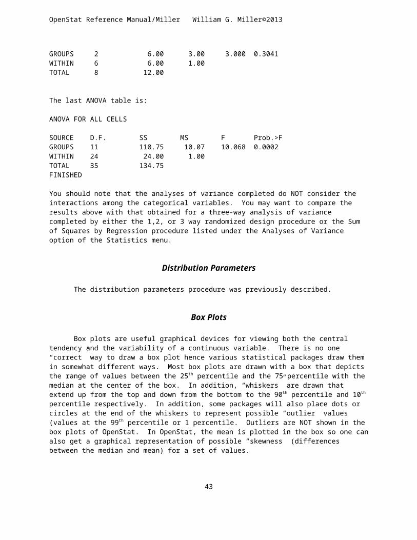
OpenStat Reference Manual/Miller William G. Miller©2013
Figure 6.11 Form for a Pie Chart
In this example we have loaded the chisqr.OPENSTAT file and have chosen to obtain a pie chart of the col variable. The result is shown below:
Figure 6.12 Pie Chart
43

OpenStat Reference Manual/Miller William G. Miller©2013
Stem and Leaf Plot
One of the earliest plots in the annals of statistics was the "Stem and Leaf" plot. This plot gives the user a view of the major values found in a frequency distribution. To illustrate this plot, we will use the file labeled "StemleafTest2.TAB. If you select this option from the Descriptive option of the Analyses menu, you will see the dialogue form below:
Figure 6.13 Stem and Leaf Form
We will choose to plot the zx100 variable to obtain the following results:
STEM AND LEAF PLOTS
Stem and Leaf Plot for variable: zx100
Frequency Stem & Leaf 1 -3 0 6 -2 0034 12 -1 0122234 5 -1 6789 71 0 0001111111222222222333333344444444444 78 0 5555555556666666677777777788888889999999 16 1 00011223 7 1 56789 2 2 03 2 2 57
Stem width = 100.00, max. leaf depth = 244

OpenStat Reference Manual/Miller William G. Miller©2013
Min. value = -299.000, Max. value = 273.600No. of good cases = 200
The results indicate that the Stem has values ranging from -300 to +200 with the second digits shown as leaves. For example, the value 111.6 has a stem of 100 and a leaf of 1. The leaf "depth" indicates the number of values that each leaf value represents. The shape of the plot is useful in examining whether the distribution is somewhat "bell" shaped, flat, skewed, etc.
Compare Observed and Theoretical Distributions
In addition to the Stem and Leaf Plot described above, one can also plot a sample distribution along with a theoretical distribution using the cumulative proportion of values in the observed distribution. To demonstrate, we will again use the same variable and file in the stem and leaf plot described above. We will examine the normal distribution values expected for the same cumulative proportions of the observed data. When you select this option from the Descriptive option, you see the form shown below:
Figure 6.14 Dialog Form for Examining Theoretical and Observed Distributions
When you click the Compute Button, you obtain the plot. Notice that our distributions are quite similar!
45

OpenStat Reference Manual/Miller William G. Miller©2013
QQ and PP Plots
In a manner similar to that shown above, one can also obtain a plot of the theoretical versus the observed data. You may select to plot actual values observed and expected or the proportions (probabilities) observed and expected. Show below is the dialogue form and a QQ plot for the save data of the previous section:
Figure 6.15 The QQ / PP Plot Specification Form
46

OpenStat Reference Manual/Miller William G. Miller©2013
Figure 6.16 A QQ Plot
Normality Tests
A large number of statistical analyses have an underlying assumption that the data analyzed or the errors in predicting the data are, in fact, normally distributed in the population from which the sample was obtained. Several tests have been developed to test this assumption. We will again use the above sample data to demonstrate these tests. The specification form and the results are shown below:
47
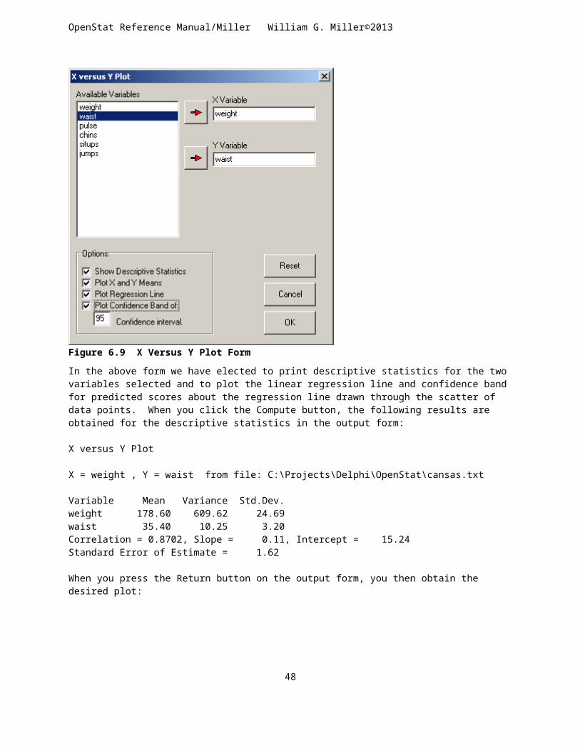
OpenStat Reference Manual/Miller William G. Miller©2013
Figure 6.17 Normality Tests
The Shapiro-Wilkes statistic indicates a relatively high probability of obtaining the sample data from a normal population. The Liliefors test statistic also suggests there is no evidence against normality. Both tests lead us to accept the hypothesis that the sample was obtained from a normally distributed population of scores.
48

OpenStat Reference Manual/Miller William G. Miller©2013
Resistant Line
Tukey (1970, Chapter 10) proposed the three point resistant line as an data analysis tool for quickly fitting a straight line to bivariate data (x and y paired data.) The data are divided into three groups of approximately equal size and sorted on the x variable. The median points of the upper and lower groups are fitted to the middle group to form two slope lines. The resulting slope line is resistant to the effects of extreme scores of either x or y values and provides a quick exploratory tool for investigating the linearity of the data. The ratio of the two slope lines from the upper and lower group medians to the middle group median provides a quick estimate of the linearity which should be approximately 1.0 for linearity. Our example uses the “Cansas.TEX” file. The dialogue for the analysis appears as:
Figure 6.18 Resistant Line Dialog
The results obtained are:
Group X Median Y Median Size 1 155.000 155.000 6 2 176.000 34.000 8 3 197.500 36.500 6
Half Slopes = -5.762 and 0.116Slope = -2.788Ratio of half slopes = -0.020Equation: y = -2.788 * X + ( -566.361)
49

OpenStat Reference Manual/Miller William G. Miller©2013
Figure 6.19 Resistant Line Plot
50

OpenStat Reference Manual/Miller William G. Miller©2013
Repeated Measures Bubble Plot
Bubble plots are useful for comparing repeated measures for multiple objects. In our example, we have multiple schools which are being compared across years for student achievement. The size of the bubbles that are plotted represent the ratio of students to teachers. We are using the BubblePlot2.TEX file in the sample data files.Shown below is the dialog for the bubble plot procedure followed by the plot and the descriptive data of the analysis:
Figure 6.20 Dialog for the Repeated Measures Bubble Plot
Figure 6.21 Bubble Plot
MEANS FOR Y AND SIZE VARIABLES
51

OpenStat Reference Manual/Miller William G. Miller©2013
Grand Mean for Y = 18.925Grand Mean for Size = 23.125
REPLICATION MEAN Y VALUES (ACROSS OBJECTS)Replication 1 Mean = 17.125Replication 2 Mean = 18.875Replication 3 Mean = 18.875Replication 4 Mean = 19.250Replication 5 Mean = 20.500
REPLICATION MEAN SIZE VALUES (ACROSS OBJECTS}Replication 1 Mean = 25.500Replication 2 Mean = 23.500Replication 3 Mean = 22.750Replication 4 Mean = 22.500Replication 5 Mean = 21.375
MEAN Y VALUES FOR EACH BUBBLE (OBJECT)Object 1 Mean = 22.400Object 2 Mean = 17.200Object 3 Mean = 19.800Object 4 Mean = 17.200Object 5 Mean = 22.400Object 6 Mean = 15.800Object 7 Mean = 20.000Object 8 Mean = 16.600
MEAN SIZE VALUES FOR EACH BUBBLE (OBJECT)Object 1 Mean = 19.400Object 2 Mean = 25.200Object 3 Mean = 23.000Object 4 Mean = 24.600Object 5 Mean = 19.400Object 6 Mean = 25.800Object 7 Mean = 23.200Object 8 Mean = 24.400
52
OpenStat Reference Manual/Miller William G. Miller©2013
Smooth Data by Averaging
Measurements made on multiple objects often contain “noise” or error variations that mask the trend of data. One method for reducing this “noise” is to smooth the data by averaging the data points. In this method, three contiguous data points are averaged to obtain a new value for the first of the three points. The next point is the average of three points, etc. across all points. Only the first and last data points are left unchanged. To illustrate this procedure, we will use the file labeled “boltsize.TEX”. The dialog is shown followed by a comparison of the original data with the smoothed data using the procedure to compare two distributions:
Figure 6.22 Dialog for Smoothing Data by Averaging
Figure 6.23 Smoothed Data Frequency Distribution Plot
53

OpenStat Reference Manual/Miller William G. Miller©2013
Figure 6.24 Cumulative Frequency of Smoothed Data
54

OpenStat Reference Manual/Miller William G. Miller©2013
X Versus Multiple Y Plot
You may have collected multiple measurements for a group of objects and wish to compare these measurements in a plot. This procedure lets you select a variable for the X axis and multiple Y variables to plot as points or lines. To illustrate we have selected a file labeled “multiplemeas.TEX” and have plotted a group of repeated measures against the first one. The dialog is shown below followed by the plot:
Figure 6.25 Dialog for an X Versus Multiple Y Plot
X VERSUS MULTIPLE Y VALUES PLOT
CORRELATION MATRIX
Correlations VAR2 VAR3 VAR4 VAR5 VAR6 VAR1 VAR2 1.000 0.255 0.542 0.302 0.577 0.325 VAR3 0.255 1.000 -0.048 0.454 0.650 0.763 VAR4 0.542 -0.048 1.000 0.125 -0.087 0.005 VAR5 0.302 0.454 0.125 1.000 0.527 0.304
55

OpenStat Reference Manual/Miller William G. Miller©2013
VAR6 0.577 0.650 -0.087 0.527 1.000 0.690 VAR1 0.325 0.763 0.005 0.304 0.690 1.000
Means
Variables VAR2 VAR3 VAR4 VAR5 VAR6 VAR1 8.894 9.682 5.021 9.721 9.451 6.639
Standard Deviations
Variables VAR2 VAR3 VAR4 VAR5 VAR6 VAR1 12.592 16.385 17.310 13.333 16.157 11.834
No. of valid cases = 30
Figure 6.26 X Versus Multiple Y Plot
56

OpenStat Reference Manual/Miller William G. Miller©2013
Compare Observed to a Theoretical Distribution
Observed data may be distributed in a manner similar to a variety of theoretical distributions. This procedure lets you plot the observed scores against various theoretical distributions to see if the data tends to be more similar to one than another. We will demonstrate using a set of simulated data that we created to follow an approximately normal distribution. We smoothed the data using the smoothing procedure and then compared the smoothed data to the normal distribution by means of this procedure. Shown below is the dialog utilized and the resulting plot of the data:
Figure 6.27 Dialog for Comparing Observed and Theoretical Distributions
Figure 6.28 Comparison of an Observed and Theoretical Distribution
57

OpenStat Reference Manual/Miller William G. Miller©2013
Multiple Groups X versus Y Plot
You may have observed objects within groups such as male and female (coded 0 and 1 for example) and wish to plot the relationship between two other measures for those groups. To demonstrate this procedure we will use the sample data file labeled “anova2.TEX” and plot the lines for the relationship of the dependent variable x and the covariate2 in the file. The dialog is shown below followed by the plot:
Figure 6.29 Dialog for Multiple Groups X Versus Y Plot
X VERSUS Y FOR GROUPS PLOT
VARIABLE MEAN STANDARED DEVIATION X 4.083 1.962 Y 3.917 1.628
58

OpenStat Reference Manual/Miller William G. Miller©2013
Figure 6.30 X Versus Y Plot for Multiple Groups
59

OpenStat Reference Manual/Miller William G. Miller©2013
VII. Correlation
The Product Moment Correlation
It seems most living creatures observe relationships, perhaps as a survival instinct. We observe signs that the weather is changing and prepare ourselves for the winter season. We observe that when seat belts are worn in cars that the number of fatalities in car accidents decrease. We observe that students that do well in one subject tend to perform will in other subjects. This chapter explores the linear relationship between observed phenomena.
If we make systematic observations of several phenomena using some scales of measurement to record our observations, we can sometimes see the relationship between them by “plotting” the measurements for each pair of measures of the observations. As a hypothetical example, assume you are a commercial artist and produce sketches for advertisement campaigns. The time given to produce each sketch varies widely depending on deadlines established by your employer. Each sketch you produce is ranked by five marketing executives and an average ranking produced (rank 1 = best, rank 5 = poorest.) You suspect there is a relationship between time given (in minutes) and the average quality ranking obtained. You decide to collect some data and observe the following:
Average Rank (Y) Minutes (X)3.8 102.6 354.0 51.8 423.0 302.6 322.8 313.2 263.6 112.8 33
Using OpenStat Descriptive menu’s Plot X vs. Y procedure to plot these values yields the scatter-plot shown on the following page. Is there a relationship between the production time and average quality ratings?
60

OpenStat Reference Manual/Miller William G. Miller©2013
Figure 7.1 Correlation Regression Line
Testing Hypotheses for Relationships Among Variables: CorrelationTo further understand and learn to interpret the product-moment correlation, OpenStat provides a means of
simulating pairs of data, plotting those pairs, drawing the “best-fitting line” to the data points and showing the marginal distributions of the X and Y variables. Go to the Simulation menu and click on the Bivariate Scatter Plot. The figure below shows a simulation for a population correlation of -.95 with population means and variances as shown. A sample of 100 cases are generated. Actual sample means and standard deviations will vary (as sample statistics do!) from the population values specified.
POPULATION PARAMETERS FOR THE SIMULATIONMean X := 100.000, Std. Dev. X := 15.000Mean Y := 100.000, Std. Dev. Y := 15.000Product-Moment Correlation := -0.900Regression line slope := -0.900, constant := 190.000SAMPLE STATISTICS FOR 100 OBSERVATIONS FROM THE POPULATIONMean X := 99.988, Std. Dev. X := 14.309Mean Y := 100.357, Std. Dev. Y := 14.581Product-Moment Correlation := -0.915Regression line slope := -0.932, constant := 193.577
61

OpenStat Reference Manual/Miller William G. Miller©2013
Figure 7.2 Simulated Bivariate Scatterplot
Simple Linear Regression
The product-moment correlation discussed in the previous section is an index of the linear relationship between two continuous variables. But what is the nature of that linear relationship? That is, what is the slope of the line and where does the line intercept the vertical (Y variable) axis? This unit will examine the straight line "fit" to data points representing observations with two variables. We will also examine how this straight line may be used for prediction purposes as well as describing the relationship to the product-moment correlation coefficient.
OpenStat contains a procedure for completing a z test for data like that presented above.Under the Statistics menu, move your mouse down to the Comparisons sub-menu, and then to the option entitled “One Sample Tests”. When the form below displays, click on the Correlation button and enter the sample value .5, the population value .6, and the sample size 50. Change the confidence level to 90.0%.Shown below is the z-test for the above data:
Figure 7.3 Single Sample Tests Form for Correlations
62

OpenStat Reference Manual/Miller William G. Miller©2013
ANALYSIS OF A SAMPLE CORRELATION
Sample Correlation = 0.600Population Correlation = 0.500Sample Size = 50z Transform of sample correlation = 0.693z Transform of population correlation = 0.549Standard error of transform = 0.146z test statistic = 0.986 with probability 0.838z value required for rejection = 1.645Confidence Interval for sample correlation = ( 0.425, 0.732)
Testing Equality of Correlations in Two Populations
Figure 7.4 Comparison of Two Independent Correlations
COMPARISON OF TWO CORRELATIONS
63

OpenStat Reference Manual/Miller William G. Miller©2013
Correlation one = 0.500Sample size one = 30Correlation two = 0.600Sample size two = 40Difference between correlations = -0.100Confidence level selected = 95z for Correlation One = 0.549z for Correlation Two = 0.693z difference = -0.144Standard error of difference = 0.253z test statistic = -0.568Probability > |z| = 0.715z Required for significance = 1.960Note: above is a two-tailed test.Confidence Limits = (-0.565, 0.338)
Differences Between Correlations in Dependent Samples
Again, OpenStat provides the computations for the difference between dependent correlations as shown in the figure below:
Figure 7.5 Comparison of Correlations for Dependent Samples
64

OpenStat Reference Manual/Miller William G. Miller©2013
COMPARISON OF TWO CORRELATIONS
Correlation x with y = 0.400Correlation x with z = 0.600Correlation y with z = 0.700Sample size = 50Confidence Level Selected = 95.0Difference r(x,y) - r(x,z) = -0.200t test statistic = -2.214Probability > |t| = 0.032t value for significance = 2.012
Partial and Semi_Partial Correlations
Partial Correlation
OpenStat provides a procedure for obtaining partial and semi-partial correlations. You can select the Analyses/Correlation/Partial procedure. We have used the cansas.tab file to demonstrate how to obtain partial and semi-partial correlations as shown below:
Figure 7.6 Form for Calculating Partial and Semi-Partial Correlations65

OpenStat Reference Manual/Miller William G. Miller©2013
Partial and Semi-Partial Correlation AnalysisDependent variable = chins
Predictor VarList:Variable 1 = weightVariable 2 = waist
Control Variables:Variable 1 = pulse
Higher order partialling at level = 2
CORRELATION MATRIX
Correlations chins weight waist pulse chins 1.000 -0.390 -0.552 0.151 weight -0.390 1.000 0.870 -0.366 waist -0.552 0.870 1.000 -0.353 pulse 0.151 -0.366 -0.353 1.000
Means
Variables chins weight waist pulse 9.450 178.600 35.400 56.100
Standard Deviations
Variables chins weight waist pulse 5.286 24.691 3.202 7.210
No. of valid cases = 20
Squared Multiple Correlation with all Variables = 0.340
Standardized Regression Coefficients: weight = 0.368 waist = -0.882 pulse = -0.026
Squared Multiple Correlation with control Variables = 0.023
Standardized Regression Coefficients: pulse = 0.151
Partial Correlation = 0.569
Semi-Partial Correlation = 0.563
F = 3.838 with probability = 0.0435, D.F.1 = 2 and D.F.2 = 16
66

OpenStat Reference Manual/Miller William G. Miller©2013
Autocorrelation
Now let us look at an example of auto-correlation. We will use a file named strikes.tab. The file contains a column of values representing the number of strikes which occurred each month over a 30 month period. Select the auto-correlation procedure from the Correlations sub-menu of the Analyses main menu. Below is a representation of the form as completed to obtain auto-correlations, partial auto-correlations, and data smoothing using both moving average smoothing and polynomial regression smoothing:
Figure 7.7 The Autocorrelation Form
When we click the Compute button, we first obtain a dialog form for setting the parameters of our moving average.In that form we first enter the number of values to include in the average from both sides of the current average value. We selected 2. Be sure and press the Enter key after entering the order value. When you do, two theta values will appear in a list box. When you click on each of those thetas, you will see a default value appear in a text box. This is the weight to assign the leading and trailing averages (first or second in our example.) In our example we have accepted the default value for both thetas (simply press the Return key to accept the default or enter a value and press the Return key.) Now press the Apply button. When you do this, the weights for all of the values (the current mean and the 1, 2, … order means) are recalculated. You can then press the OK button to proceed with the process.
67

OpenStat Reference Manual/Miller William G. Miller©2013
Figure 7.8 Moving Average Form
The procedure then plots the original (30) data points and their moving average smoothed values. Since we also asked for a projection of 5 points, they too are plotted. The plot should look like that shown below:
Figure 7.9 Smoothed Plot Using Moving Average
68

OpenStat Reference Manual/Miller William G. Miller©2013
We notice that there seems to be a “wave” type of trend with a half-cycle of about 15 months. When we press the Return button on the plot of points we next get the following:
Figure 7.10 Plot of Residuals Obtained Using Moving Averages
This plot shows the original points and the difference (residual) of the smoothed values from the original. At this point, the procedure replaces the original points with the smoothed values. Press the Return button and you next obtain the following:
Figure 7.11 Polynomial Regression Smoothing Form
This is the form for specifying our next smoothing choice, the polynomial regression smoothing. We have elected to use a polynomial value of 2 which will result in a model for a data point Yt-1 = B * t2 + C for each data point. Click the OK button to proceed. You then obtain the following result:
69

OpenStat Reference Manual/Miller William G. Miller©2013
Figure 7.12 Plot of Polynomial Smoothed Points
It appears that the use of the second order polynomial has “removed” the cyclic trend we saw in the previously smoothed data points. Click the return key to obtain the next output as shown below:
Figure 7.13 Plot of Residuals from Polynomial Smoothing
This result shows the previously smoothed data points and the residuals obtained by subtracting the polynomial smoothed points from those previous points. Click the Return key again to see the next output shown below:
70
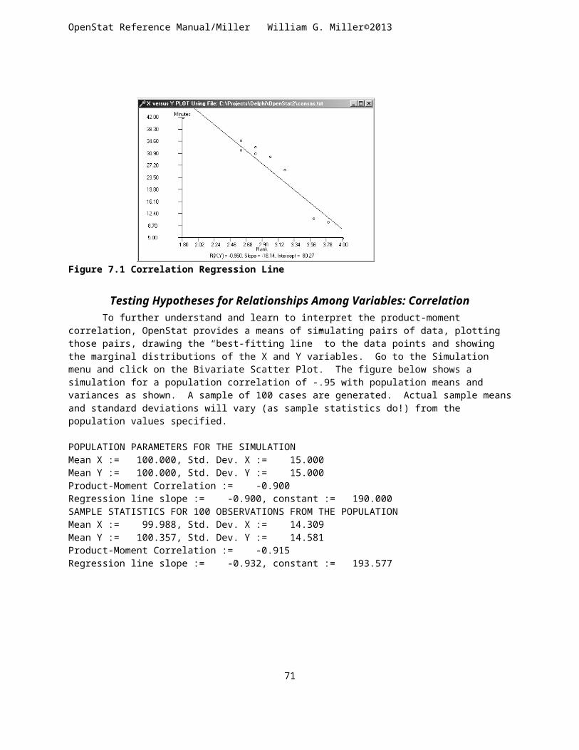
OpenStat Reference Manual/Miller William G. Miller©2013
Overall mean = 4532.604, variance = 11487.241Lag Rxy MeanX MeanY Std.Dev.X Std.Dev.Y Cases LCL UCL
0 1.0000 4532.6037 4532.6037 109.0108 109.0108 30 1.0000 1.0000 1 0.8979 4525.1922 4537.3814 102.9611 107.6964 29 0.7948 0.9507 2 0.7964 4517.9688 4542.3472 97.0795 106.2379 28 0.6116 0.8988 3 0.6958 4510.9335 4547.5011 91.3660 104.6337 27 0.4478 0.8444 4 0.5967 4504.0864 4552.8432 85.8206 102.8825 26 0.3012 0.7877 5 0.4996 4497.4274 4558.3734 80.4432 100.9829 25 0.1700 0.7287 6 0.4050 4490.9565 4564.0917 75.2340 98.9337 24 0.0524 0.6679 7 0.3134 4484.6738 4569.9982 70.1928 96.7340 23 -0.0528 0.6053 8 0.2252 4478.5792 4576.0928 65.3196 94.3825 22 -0.1470 0.5416 9 0.1410 4472.6727 4582.3755 60.6144 91.8784 21 -0.2310 0.4770 10 0.0611 4466.9544 4588.8464 56.0772 89.2207 20 -0.3059 0.4123 11 -0.0139 4461.4242 4595.5054 51.7079 86.4087 19 -0.3723 0.3481 12 -0.0836 4456.0821 4602.3525 47.5065 83.4415 18 -0.4309 0.2852
In the output above we are shown the auto-correlations obtained between the values at lag 0 and those at lags 1 through 12. The procedure limited the number of lags automatically to insure a sufficient number of cases upon which to base the correlations. You can see that the upper and lower 95% confidence limits increases as the number of cases decreases. Click the Return button on the output form to continue the process.
Matrix of Lagged Variable: VAR00001 with 30 valid cases.
Variables Lag 0 Lag 1 Lag 2 Lag 3 Lag 4 Lag 0 1.000 0.898 0.796 0.696 0.597 Lag 1 0.898 1.000 0.898 0.796 0.696 Lag 2 0.796 0.898 1.000 0.898 0.796 Lag 3 0.696 0.796 0.898 1.000 0.898 Lag 4 0.597 0.696 0.796 0.898 1.000 Lag 5 0.500 0.597 0.696 0.796 0.898 Lag 6 0.405 0.500 0.597 0.696 0.796 Lag 7 0.313 0.405 0.500 0.597 0.696 Lag 8 0.225 0.313 0.405 0.500 0.597 Lag 9 0.141 0.225 0.313 0.405 0.500 Lag 10 0.061 0.141 0.225 0.313 0.405 Lag 11 -0.014 0.061 0.141 0.225 0.313 Lag 12 -0.084 -0.014 0.061 0.141 0.225
Variables Lag 5 Lag 6 Lag 7 Lag 8 Lag 9 Lag 0 0.500 0.405 0.313 0.225 0.141 Lag 1 0.597 0.500 0.405 0.313 0.225 Lag 2 0.696 0.597 0.500 0.405 0.313 Lag 3 0.796 0.696 0.597 0.500 0.405 Lag 4 0.898 0.796 0.696 0.597 0.500 Lag 5 1.000 0.898 0.796 0.696 0.597 Lag 6 0.898 1.000 0.898 0.796 0.696 Lag 7 0.796 0.898 1.000 0.898 0.796 Lag 8 0.696 0.796 0.898 1.000 0.898 Lag 9 0.597 0.696 0.796 0.898 1.000 Lag 10 0.500 0.597 0.696 0.796 0.898 Lag 11 0.405 0.500 0.597 0.696 0.796 Lag 12 0.313 0.405 0.500 0.597 0.696
71

OpenStat Reference Manual/Miller William G. Miller©2013
Variables Lag 10 Lag 11 Lag 12 Lag 0 0.061 -0.014 -0.084 Lag 1 0.141 0.061 -0.014 Lag 2 0.225 0.141 0.061 Lag 3 0.313 0.225 0.141 Lag 4 0.405 0.313 0.225 Lag 5 0.500 0.405 0.313 Lag 6 0.597 0.500 0.405 Lag 7 0.696 0.597 0.500 Lag 8 0.796 0.696 0.597 Lag 9 0.898 0.796 0.696 Lag 10 1.000 0.898 0.796 Lag 11 0.898 1.000 0.898 Lag 12 0.796 0.898 1.000
The above data presents the inter-correlations among the 12 lag variables. Click the output form’s Return button to obtain the next output:
Partial Correlation Coefficients with 30 valid cases.
Variables Lag 0 Lag 1 Lag 2 Lag 3 Lag 4 1.000 0.898 -0.051 -0.051 -0.052
Variables Lag 5 Lag 6 Lag 7 Lag 8 Lag 9 -0.052 -0.052 -0.052 -0.052 -0.051
Variables Lag 10 Lag 11 -0.051 -0.051
The partial auto-correlation coefficients represent the correlation between lag 0 and each remaining lag with previous lag values partialled out. For example, for lag 2 the correlation of -0.051 represents the correlation between lag 0 and lag 2 with lag 1 effects removed. Since the original correlation was 0.796, removing the effect of lag 1 made a considerable impact. Again click the Return button on the output form. Next you should see the following results:
72

OpenStat Reference Manual/Miller William G. Miller©2013
Figure 7.14 Auto and Partial Autocorrelation Plot
This plot or “correlogram” shows the auto-correlations and partial auto-correlations obtained in the analysis. If only “noise” were present, the correlations would vary around zero. The presence of large values is indicative of trends in the data.
73

OpenStat Reference Manual/Miller William G. Miller©2013
VIII. Comparisons
One Sample Tests
OpenStat provides the ability to perform tests of hypotheses based on a single sample. Typically the user is interested in testing the hypothesis that 1. a sample mean does not differ from a specified hypothesized mean,2. a sample proportion does not differ from a specified population proportion,3. a sample correlation does not differ from a specified population correlation, or4. a sample variance does not differ from a specified population variance.
The One Sample Test for means, proportions, correlations and variances is started by selecting the Comparisons option under the Statistics menu and moving the mouse to the One Sample Tests option which you then click with the left mouse button. If you do this you will then see the specification form for your comparison as seen below. In this form there is a button corresponding to each of the above type of comparison. You click the one of your choice. There are also text boxes in which you enter the sample statistics for your test and select the confidence level desired for the test. We will illustrate each test. In the first one we will test the hypothesis thata sample mean of 105 does not differ from a hypothesized population mean of 100. The standard deviation is estimated to be 15 and our sample size is 20.
Figure 8.1 Single Sample Tests Dialog Form
When we click the Continue button on the form we then obtain our results in an output form as shown below:
ANALYSIS OF A SAMPLE MEAN
Sample Mean = 105.000Population Mean = 100.000Sample Size = 20Standard error of Mean = 3.354t test statistic = 1.491 with probability 0.152t value required for rejection = 2.093Confidence Interval = (97.979,112.021)
74
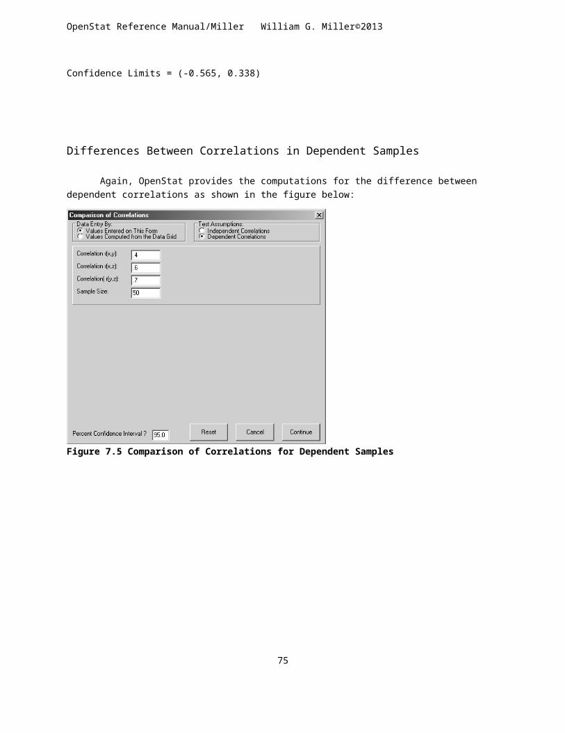
OpenStat Reference Manual/Miller William G. Miller©2013
We notice that our sample mean is “captured” in the 95 percent confidence interval and this would lead us to accept the null hypothesis that the sample is not different from that expected by chance alone from a population with mean 100.
Now let us perform a test of a sample proportion. Assume we have an elective high school course in Spanish I. We notice that the proportion of 30 students in the class that are female is only 0.4 (12 students) yet the population of high school students in composed of 50% male and 50% female. Is the proportion of females enrolled in the class representative of a random sample from the population? To test the hypothesis that the proportion of .4 does not differ from the population proportion of .5 we click the proportion button of the form and enter our sample data as shown below:
Figure 8.2 Single Sample Proportion Test
When we click the Continue button we see the results as shown below:
ANALYSIS OF A SAMPLE PROPORTION
Two tailed test at the 0.950 confidence levelSample Proportion = 0.9705882Population Proportion = 0.9500000Sample Size = 340Standard error of sample proportion = 0.0091630z test statistic = 2.2469 with probability > z = 0.0123z test statistic = 2.2469 with probability < z = 0.9877z value required for rejection = 2.4673Confidence Interval = (0.9526290,0.9885474)
We note that the z statistic obtained for our sample has a fairly low probability of occurring by chance when drawn from a population with a proportion of .5 so we are led to reject the null hypothesis.
We examined the test for a hypothesis about a sample correlation being obtained from a population with a given correlation. See the Correlation chapter to review that test.
It occurs to a teacher that perhaps her Spanish students are from a more homogeneous population than that of the validation study reported in a standardized Spanish aptitude test. If that were the case, the correlation she observed might well be attenuated due to the differences in variances. In her class of thirty students she observed a
75

OpenStat Reference Manual/Miller William G. Miller©2013
sample variance of 25 while the validation study for the instrument reported a variance of 36. Let’s examine the test for the hypothesis that her sample variance does not differ significantly from the “population” value. Again we invoke the One Sample Test from the Univariate option of the Analyses menu and complete the form as shown below:
Figure 8.3 Single Sample Variance Test
Upon clicking the Continue button our teacher obtains the following results in the output form:
ANALYSIS OF A SAMPLE VARIANCE
Sample Variance = 25.000Population Variance = 36.000Sample Size = 30Chi-square statistic = 20.139 with probability > chisquare = 0.889 and D.F. = 29Chi-square value required for rejection = 16.035Chi-square Confidence Interval = (45.725,16.035)Variance Confidence Interval = (15.856,45.215)
The chi-square statistic obtained leads our teacher to accept the hypothesis of no difference between her sample variance and the population variance. Note that the population variance is clearly within the 95% confidence interval for the sample variance.
Proportion Differences
A most common research question arises when an investigator has obtained two sample proportions. One asks whether or not the two sample proportions are really different considering that they are based on observations drawn randomly from a population. For example, a school nurse observes during the flu season that 13 eighth grade students are absent due to flu symptoms while only 8 of the ninth grade students are absent. The class sizes of the two grades are 110 and 121 respectively. The nurse decides to test the hypothesis that the two proportions (.118 and .066) do not differ significantly using the OpenStat program. The first step is to start the Proportion Differences procedure by clicking on the Analyses menu, moving the mouse to the Univariate option and the clicking on the Proportion Differences option. The specification form for the test then appears. We will enter the required values directly on the form and assume the samples are independent random samples from a population of eighth and ninth grade students.
76

OpenStat Reference Manual/Miller William G. Miller©2013
Figure 8.4 Test of Equality of Two Proportions
When the nurse clicks the Continue button the following results are shown in the Output form:
COMPARISON OF TWO PROPORTIONS
Test for Difference Between Two Independent Proportions
Entered Values
Sample 1: Frequency = 13 for 110 cases.Sample 2: Frequency = 8 for 121 cases.Proportion 1 = 0.118, Proportion 2 = 0.066, Difference = 0.052Standard Error of Difference = 0.038Confidence Level selected = 95.0z test statistic = 1.375 with probability = 0.0846z value for confidence interval = 1.960Confidence Interval: ( -0.022, 0.126)
The nurse notices that the value of zero is within the 95% confidence interval as therefore accepts the null hypothesis that the two proportions are not different than that expected due to random sampling variability. What would the nurse conclude had the 80.0% confidence level been chosen?
If the nurse had created a data file with the above data entered into the grid such as:
CASE/VAR FLU GROUPCASE 1 0 1CASE 2 1 1I. --
CASE 110 0 1CASE 111 0 2S --
77

OpenStat Reference Manual/Miller William G. Miller©2013
CASE 231 1 2
then the option would have been to analyze data in a file.
In this case, the absence or presence of flu symptoms for the student are entered as zero (0) or one (1) and the grade is coded as 1 or 2. If the same students, say the eighth grade students, are observed at weeks 10 and 15 during the semester, than the test assumptions would be changed to Dependent Proportions. In that case the form changes again to accommodate two variables coded zero and one to reflect the observations for each student at weeks 10 and 15.
Figure 8.5 Test of Equality of Two Proportions Form
t-Tests
Among the comparison techniques the “Student” t-test is one of the most commonly employed. One may test hypotheses regarding the difference between population means for independent or dependent samples which meet or do not meet the assumptions of homogeneity of variance. To complete a t-test, select the t-test option from the Comparisons sub-menu of the Statistics menu. You will see the form below:
78

OpenStat Reference Manual/Miller William G. Miller©2013
Figure 8.6 Comparison of Two Sample Means Form
Notice that you can enter values directly on the form or from a file read into the data grid. If you elect to read data from the data grid by clicking the button corresponding to “Values Computed from the Data Grid” you will see that the form is modified as shown below.
Figure 8.7 Comparison of Two Sample Means
We will analyze data stored in the Hinkle247.tab file.
79

OpenStat Reference Manual/Miller William G. Miller©2013
Once you have entered the variable name and the group code name you click the Continue button. The following results are obtained for the above analysis:
COMPARISON OF TWO MEANS
Variable Mean Variance Std.Dev. S.E.Mean NGroup 1 49.44 107.78 10.38 3.46 9Group 2 68.88 151.27 12.30 4.35 8Assuming = variances, t = -3.533 with probability = 0.0030 and 15 degrees of freedomDifference = -19.43 and Standard Error of difference = 5.50Confidence interval = ( -31.15, -7.71)Assuming unequal variances, t = -3.496 with probability = 0.0034 and 13.82 degrees of freedomDifference = -19.43 and Standard Error of difference = 5.56Confidence interval = ( -31.37, -7.49)F test for equal variances = 1.404, Probability = 0.3209
The F test for equal variances indicates it is reasonable to assume the sampled populations have equal variances hence we would report the results of the first test. Since the probability of the obtained statistic is rather small (0.003), we would likely infer that the samples were drawn from two different populations. Note that the confidence interval for the observed difference is reported.
80

One, Two or Three Way Analysis of Variance
An experiment often involves the observation of some continuous variable under one or more controlled conditions or factors. For example, one might observe two randomly assigned groups of subjects performance under two or more levels of some treatment. The question posed is whether or not the means of the populations under the various levels of treatment are equal. Of course, if there is only two levels of treatment for one factor then we could analyze the data with the t-test described above. In fact, we will analyze the same “Hinkle.txt” file data with the anova program. Select the “One, Two or Three Way ANOVA” option from the Comparisons sub-menu of the Statistics menu. You will see the form below:
Figure 8.8 One, Two or Three Way ANOVA Dialog
Since our first example involves one factor only we will click the VAR1 variable name and click the right arrow button to place it in the Dependent Variable box. We then click the “group” variable label and the right arrow to place it in the Factor 1 Variable box. We will assume the levels represent fixed treatment levels. We will also elect to plot the sample means for each level using three dimension bars. When we click the Continue button we will obtain the results shown below:
ONE WAY ANALYSIS OF VARIANCE RESULTSDependent variable is: VAR1, Independent variable is: group
---------------------------------------------------------------------SOURCE D.F. SS MS F PROB.>F OMEGA SQR.---------------------------------------------------------------------BETWEEN 1 1599.02 1599.02 12.49 0.00 0.40WITHIN 15 1921.10 128.07TOTAL 16 3520.12---------------------------------------------------------------------
MEANS AND VARIABILITY OF THE DEPENDENT VARIABLE FOR LEVELS OF THE INDEPENDENT VARIABLE
81
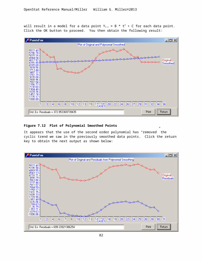
---------------------------------------------------------------------GROUP MEAN VARIANCE STD.DEV. N--------------------------------------------------------------------- 1 49.44 107.78 10.38 9 2 68.88 151.27 12.30 8---------------------------------------------------------------------TOTAL 58.59 220.01 14.83 17---------------------------------------------------------------------
TESTS FOR HOMOGENEITY OF VARIANCE---------------------------------------------------------------------Hartley Fmax test statistic = 1.40 with deg.s freedom: 2 and 8.Cochran C statistic = 0.58 with deg.s freedom: 2 and 8.Bartlett Chi-square = 0.20 with 1 D.F. Prob. = 0.347---------------------------------------------------------------------
In this example, we note that the F statistic (12.49) is simply the square of the previously observed t statistic (within rounding error.) The Bartlett Chi-square test for homogeneity of variance and the Hartley Fmax test also agree approximately with the F statistic for equal variance in the t-test procedure.
The plot of the sample means obtained in our analysis are shown below:
Figure 8.9 Plot of Sample Means From a One-Way ANOVA
Now let us run an example of an analysis with one fixed and one random factor. We will use the data file named “Threeway.txt” which could also serve to demonstrate a three way analysis of variance (with fixed or random effects.) We will assume the row variable is fixed and the column variable is a random level. We select the One, Two and Three Way ANOVA option from the Comparisons sub-menu of the Statistics menu. The figure below shows how we specified the variables and their types:
82

Figure 8.10 Specifications for a Two-Way ANOVA
Now when we click the Continue button we obtain:
Two Way Analysis of Variance
Variable analyzed: X
Factor A (rows) variable: Row (Fixed Levels)Factor B (columns) variable: Col (Fixed Levels)
SOURCE D.F. SS MS F PROB.> F Omega Squared
Among Rows 1 12.250 12.250 5.765 0.022 0.074Among Columns 1 42.250 42.250 19.882 0.000 0.293Interaction 1 12.250 12.250 5.765 0.022 0.074Within Groups 32 68.000 2.125Total 35 134.750 3.850
Omega squared for combined effects = 0.441
Note: Denominator of F ratio is MSErr
Descriptive Statistics
GROUP Row Col. N MEAN VARIANCE STD.DEV.Cell 1 1 9 3.000 1.500 1.225Cell 1 2 9 4.000 1.500 1.225Cell 2 1 9 3.000 3.000 1.732Cell 2 2 9 6.333 2.500 1.581Row 1 18 3.500 1.676 1.295Row 2 18 4.667 5.529 2.351
83

Col 1 18 3.000 2.118 1.455Col 2 18 5.167 3.324 1.823TOTAL 36 4.083 3.850 1.962
TESTS FOR HOMOGENEITY OF VARIANCE---------------------------------------------------------------------Hartley Fmax test statistic = 2.00 with deg.s freedom: 4 and 8.Cochran C statistic = 0.35 with deg.s freedom: 4 and 8.Bartlett Chi-square statistic = 3.34 with 3 D.F. Prob. = 0.658---------------------------------------------------------------------
You will note that the denominator of the F statistic for the two main effects are different. For the fixed effects factor (A or rows) the mean square for interaction is used as the denominator while for the random effects factor and interaction of fixed with random factors the mean square within cells is used.
84

Analysis of Variance - Treatments by Subjects Design
An Example
To perform a Treatments by Subjects analysis of variance, we will use a sample data file labeled “ABRData.txt” which you can find as a “.tab” type of file in your sample of data files. We open the file and select the option “Within Subjects Anova” in the Comparisons sub-menu under the Statistics menu. The figure below is then completed as shown:
Figure 8.11 Within Subjects ANOVA Dialog
Notice that the repeated measures are the columns labeled C1 through C4. You will also note that this same procedure will report intraclass reliability estimates if elected. If you now click the Compute button, you obtain the results shown below:
Treatments by Subjects (AxS) ANOVA Results.
Data File = C:\Projects\Delphi\OpenStat\ABRData.txt
-----------------------------------------------------------SOURCE DF SS MS F Prob. > F-----------------------------------------------------------SUBJECTS 11 181.000 330.500WITHIN SUBJECTS 36 1077.000 29.917 TREATMENTS 3 991.500 330.500 127.561 0.000 RESIDUAL 33 85.500 2.591-----------------------------------------------------------TOTAL 47 1258.000 26.766
85

-----------------------------------------------------------
TREATMENT (COLUMN) MEANS AND STANDARD DEVIATIONSVARIABLE MEAN STD.DEV.C1 16.500 2.067C2 11.500 2.431C3 7.750 2.417C4 4.250 2.864
Mean of all scores = 10.000 with standard deviation = 5.174
BOX TEST FOR HOMOGENEITY OF VARIANCE-COVARIANCE MATRIX
SAMPLE COVARIANCE MATRIX with 12 valid cases.
Variables C1 C2 C3 C4 C1 4.273 2.455 1.227 1.318 C2 2.455 5.909 4.773 5.591 C3 1.227 4.773 5.841 5.432 C4 1.318 5.591 5.432 8.205
ASSUMED POP. COVARIANCE MATRIX with 12 valid cases.
Variables C1 C2 C3 C4 C1 6.057 0.693 0.693 0.693 C2 0.114 5.977 0.614 0.614 C3 0.114 0.103 5.914 0.551 C4 0.114 0.103 0.093 5.863
Determinant of variance-covariance matrix = 81.7Determinant of homogeneity matrix = 1.26E3ChiSquare = 108.149 with 8 degrees of freedomProbability of larger chisquare = 9.66E-7
86

One Between, One Repeated Design
An Example Mixed Design
We select the AxS ANOVA option in the Comparisons sub-menu of the Statistics menu and complete the specifications on the form as show below:
Figure 8.12 Treatment by Subjects ANOVA Dialog
When the Compute button is clicked you should see these results:
87

ANOVA With One Between Subjects and One Within Subjects Treatments
------------------------------------------------------------------Source df SS MS F Prob.------------------------------------------------------------------Between 11 181.000 Groups (A) 1 10.083 10.083 0.590 0.4602 Subjects w.g. 10 170.917 17.092
Within Subjects 36 1077.000 B Treatments 3 991.500 330.500 128.627 0.0000 A X B inter. 3 8.417 2.806 1.092 0.3677 B X S w.g. 30 77.083 2.569
TOTAL 47 1258.000------------------------------------------------------------------MeansTRT. B 1 B 2 B 3 B 4 TOTAL A 1 16.167 11.000 7.833 3.167 9.542 2 16.833 12.000 7.667 5.333 10.458TOTAL 16.500 11.500 7.750 4.250 10.000
Standard DeviationsTRT. B 1 B 2 B 3 B 4 TOTAL A 1 2.714 2.098 2.714 1.835 5.316 2 1.329 2.828 2.338 3.445 5.099TOTAL 2.067 2.431 2.417 2.864 5.174
Notice there appears to be no significant difference between the two groups of subjects but that within the groups, the first two treatment means appear to be significantly larger than the last two.
Since we elected to plot the means, we would also obtain the figure shown below:
88

Figure 8.13 Plot of Treatment by Subjects ANOVA Means
The graphics again demonstrate the greatest differences appear to be among the repeated measures and not the groups (A1 and A2.)
You may also have a design with two between-groups factors and repeated measures within each cell composed of subjects randomly assigned to the factor A and factor B level combinations. If you have such a design, you can employ the AxBxR Anova procedure in the OpenStat package.
89

Two Factor Repeated Measures Analysis
Repeated measures designs have the advantage that the error terms are typically smaller that designs using independent groups of observations. This was true for the Student t-test using matched or correlated scores. On the down-side, repeated measures on the same objects pose a special problem, particularly when the objects are human subjects. The main problem is "practice" or "learning" effects that may be greater for one treatment level than another. These effects are completely confounded with the actual treatment effects. While random or counter-balanced assignment of the treatments may reduce the cumulative effects to some degree, it does not remove the effects specific to a given treatment. It is also assumed that the covariance matrices are equal among the treatment levels. Users of these designs with human subjects should be careful to minimize the practice effects. This can sometimes be done by having subjects do tasks that are similar to those in the actual experiment before beginning trials of the experiment.
In this analysis, subjects (or objects) are observed (measured) under two different treatment levels (Factors A and B levels) . For example, there might be two levels of a Factor A and three levels of a Factor B for a total of 2 x 3 = 6 treatment level combinations. Each subject would be obnserved 6 times in all. There must be the same subjects in each of the combinations.
The data file analyzed must consist of 4 columns of information for each observation: a variable containing an integer identification code for the subject (1..N), an integer from 1 to A for the treatment level of A, an integer from 1 to B for the treatment level of the Factor B, and a floating point variable for the observation (measurement).
A sample file (tworepeated.tex or tworepeated.TAB) was created from the example given by Quinn McNemar in his text book "Psychological Statistics", fourth edition, John Wiley and Sons, Inc., 1969, page 367. The data represent an experiment in which four subjects are observed under two levels of illumination and three levels of Albedo (Factors A and B.) The data file therefore contains 24 observations (4 x 2 x 3.) The analysis is initiated by loading the file and clicking on the "Two Within Subjects" option in the Analyses of Variance menu. The form which appears is shown below. Notice that the options have been selected to plot means of the two main effects and the interaction effects. An option has also been clicked to obtain post-hoc comparisons among the 6 means for the treatment combinations. When the "Compute" button is clicked the following output is obtained:
90

Figure 8.14 Dialog for the Two-Way Repeated Measures ANOVA
91

Figure 8.15 Plot of Factor A Means in the Two-Way Repeated Measures Analysis
92

Figure 8.16 Plot of Factor B in the Two-Way Repeated Measures Analysis
93

Figure 8.17 Plot of Factor A and Factor B Interaction in the Two-Way Repeated Measures Analysis
-------------------------------------------------------------------SOURCE DF SS MS F Prob.>F-------------------------------------------------------------------Factor A 1 204.167 204.167 9.853 0.052Factor B 2 8039.083 4019.542 24.994 0.001Subjects 3 1302.833 434.278A x B Interaction 2 46.583 23.292 0.803 0.491A x S Interaction 3 62.167 20.722B x S Interaction 6 964.917 160.819A x B x S Inter. 6 174.083 29.01-------------------------------------------------------------------Total 23 10793.833-------------------------------------------------------------------Group 1 : Mean for cell A 1 and B 1 = 17.250
94

Group 2 : Mean for cell A 1 and B 2 = 26.000Group 3 : Mean for cell A 1 and B 3 = 60.250Group 4 : Mean for cell A 2 and B 1 = 20.750Group 5 : Mean for cell A 2 and B 2 = 35.750Group 6 : Mean for cell A 2 and B 3 = 64.500
Means for Factor AGroup 1 Mean = 34.500Group 2 Mean = 40.333
Means for Factor BGroup 1 Mean = 19.000Group 2 Mean = 30.875Group 3 Mean = 62.375
The above results reflect possible significance for the main effects of Factors A and B but not for the interaction. The F ratio of the Factor A is obtained by dividing the mean square for Factor A by the mean square for interaction of subjects with Factor A. In a similar manner, the F ratio for Factor B is the ratio of the mean square for Factor B to the mean square of the interaction of Factor B with subjects. Finally, the F ratio for the interaction of Factor A with Factor B uses the triple interaction of A with B with Subjects as the denominator.
Between 5 or 6 of the post-hoc comparisons were not significant among the 15 possible comparisons among means using the 0.05 level for rejection of the hypothesis of no difference.
95

Nested Factors Analysis Of Variance Design
Shown below is an example of a nested analysis using the file ABNested.tab.. When you select this analysis, you see the dialog below:
Figure 8.18 The Nested ANOVA Dialog
The results are shown below:
NESTED ANOVA by Bill MillerFile Analyzed: C:\Documents and Settings\Owner\My Documents\Projects\Clanguage\OpenStat\ABNested.tab
CELL MEANSA LEVEL B LEVEL MEAN STD.DEV. 1 1 2.667 1.528 1 2 3.333 1.528 1 3 4.000 1.732
2 4 3.667 1.528 2 5 4.000 1.000 2 6 5.000 1.000
3 7 3.667 1.155 3 8 5.000 1.000 3 9 6.333 0.577
96

A MARGIN MEANSA LEVEL MEAN STD.DEV. 1 3.333 1.500 2 4.222 1.202 3 5.000 1.414
GRAND MEAN = 4.185
ANOVA TABLESOURCE D.F. SS MS F PROB.A 2 12.519 6.259 3.841 0.041B(A) 6 16.222 2.704 1.659 0.189w.cells 18 29.333 1.630Total 26 58.074
Of course, if you elect to plot the means, additional graphical output is included.
97

A, B and C Factors with B Nested in A
Shown below is the dialog for this ANOVA design and the results of analyzing the file ABCNested.TAB:
Figure 8.19 Three Factor Nested ANOVA Dialog
The results are:
NESTED ANOVA by Bill MillerFile Analyzed: C:\Documents and Settings\Owner\My Documents\Projects\Clanguage\OpenStat\ABCNested.TAB
CELL MEANSA LEVEL B LEVEL C LEVEL MEAN STD.DEV. 1 1 1 2.667 1.528 1 1 2 3.333 1.155 1 2 1 3.333 1.528 1 2 2 3.667 2.082 1 3 1 4.000 1.732 1 3 2 5.000 1.732
2 4 1 3.667 1.528 2 4 2 4.667 1.528 2 5 1 4.000 1.000 2 5 2 4.667 0.577 2 6 1 5.000 1.000 2 6 2 3.000 1.000
3 7 1 3.667 1.155 3 7 2 2.667 1.155
98

3 8 1 5.000 1.000 3 8 2 6.000 1.000 3 9 1 6.667 1.155 3 9 2 6.333 0.577
A MARGIN MEANSA LEVEL MEAN STD.DEV. 1 3.667 1.572 2 4.167 1.200 3 5.056 1.731
B MARGIN MEANSB LEVEL MEAN STD.DEV. 1 3.000 1.265 2 3.500 1.643 3 4.500 1.643 4 4.167 1.472 5 4.333 0.816 6 4.000 1.414 7 3.167 1.169 8 5.500 1.049 9 6.500 0.837
C MARGIN MEANSC LEVEL MEAN STD.DEV. 1 4.222 1.577 2 4.370 1.644
AB MEANSA LEVEL B LEVEL MEAN STD.DEV. 1 1 3.000 1.265 1 2 3.500 1.643 1 3 4.500 1.643
2 4 4.167 1.472 2 5 4.333 0.816 2 6 4.000 1.414
3 7 3.167 1.169 3 8 5.500 1.049 3 9 6.500 0.837
AC MEANSA LEVEL C LEVEL MEAN STD.DEV. 1 1 3.333 1.500 1 2 4.000 1.658
2 1 4.222 1.202 2 2 4.111 1.269
3 1 5.111 1.616 3 2 5.000 1.936
99

GRAND MEAN = 4.296
ANOVA TABLESOURCE D.F. SS MS F PROB.A 2 17.815 8.907 5.203 0.010B(A) 6 42.444 7.074 4.132 0.003C 1 0.296 0.296 0.173 0.680AxC 2 1.815 0.907 0.530 0.593B(A) x C 6 11.556 1.926 1.125 0.368w.cells 36 61.630 1.712Total 53 135.259
100

Latin and Greco-Latin Square Designs
We have prepared an example file for you to analyze with OpenStat. Open the file labeled LatinSqr.TAB in your set of sample data files. We have entered four cases for each unit in our design for instructional mode, college and home residence. Once you have loaded the file, select the Latin squares designs option under the sub-menu for comparisons under the Analyses menu. You should see the form below for selecting the Plan 1 analysis.
Figure 8.20 Latin and Greco-Latin Squares Dialog
When you have selected Plan 1 for the analysis, click the OK button to continue. You will then see the form below for entering the specifications for your analysis. We have entered the variables for factors A, B and C and entered the number of cases for each unit:
101

Figure 8.21 Latin Squares Analysis Dialog
We have completed the entry of our variables and the number of cases and are ready to continue.When you press the OK button, the following results are presented on the output page:
102

Latin Square Analysis Plan 1 Results
-----------------------------------------------------------Source SS DF MS F Prob.>F-----------------------------------------------------------Factor A 92.389 2 46.194 12.535 0.000Factor B 40.222 2 20.111 5.457 0.010Factor C 198.722 2 99.361 26.962 0.000Residual 33.389 2 16.694 4.530 0.020Within 99.500 27 3.685Total 464.222 35-----------------------------------------------------------
Experimental Design------------------------------Instruction 1 2 3 ------------------------------ College 1 C2 C3 C1 2 C3 C1 C2 3 C1 C2 C3------------------------------
Cell means and totals--------------------------------------------------Instruction 1 2 3 Total-------------------------------------------------- College 1 2.750 10.750 3.500 5.667 2 8.250 2.250 1.250 3.917 3 1.500 1.500 2.250 1.750 Total 4.167 4.833 2.333 3.778 --------------------------------------------------
-------------------------------------------------- Residence 1 2 3 Total-------------------------------------------------- 2.417 1.833 7.083 3.778 --------------------------------------------------
A partial test of the interaction effects can be made by the ratio of the MS for residual to the MS within cells. In our example, it appears that our assumptions of no interaction effects may be in error. In this case, the main effects may be confounded by interactions among the factors. The results may never the less suggest differences do exist and we should complete another balanced experiment to determine the interaction effects.
103
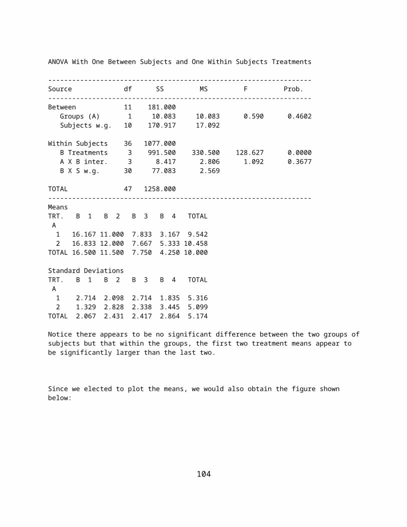
Plan 2
We have included the file “LatinSqr2.TAB” as an example for analysis. Load the file in the grid and select the Latin Square Analyses, Plan 2 design. The form below shows the entry of the variables and the sample size for the analysis:
Figure 8.22 Four Factor Latin Square Design Dialog
When you click the OK button, you will see the following results:
Latin Square Analysis Plan 2 Results
-----------------------------------------------------------Source SS DF MS F Prob.>F-----------------------------------------------------------Factor A 148.028 2 74.014 20.084 0.000Factor B 5.444 2 2.722 0.739 0.483Factor C 66.694 2 33.347 9.049 0.000
104

Factor D 18.000 1 18.000 4.884 0.031A x D 36.750 2 18.375 4.986 0.010B x D 75.000 2 37.500 10.176 0.000C x D 330.750 2 165.375 44.876 0.000Residual 66.778 4 16.694 4.530 0.003Within 199.000 54 3.685Total 946.444 71-----------------------------------------------------------
Experimental Design for block 1------------------------------ Drug 1 2 3 ------------------------------ Hospital 1 C2 C3 C1 2 C3 C1 C2 3 C1 C2 C3------------------------------
Experimental Design for block 2------------------------------ Drug 1 2 3 ------------------------------ Hospital 1 C2 C3 C1 2 C3 C1 C2 3 C1 C2 C3------------------------------
BLOCK 1
Cell means and totals-------------------------------------------------- Drug 1 2 3 Total-------------------------------------------------- Hospital 1 2.750 10.750 3.500 5.667 2 8.250 2.250 1.250 3.917 3 1.500 1.500 2.250 1.750 Total 4.167 4.833 2.333 4.278 --------------------------------------------------
BLOCK 2
Cell means and totals-------------------------------------------------- Drug 1 2 3 Total-------------------------------------------------- Hospital 1 9.250 2.250 3.250 4.917 2 3.750 4.500 11.750 6.667 3 2.500 3.250 2.500 2.750
105

Total 5.167 3.333 5.833 4.278 --------------------------------------------------
-------------------------------------------------- Category 1 2 3 Total-------------------------------------------------- 2.917 4.958 4.958 4.278 --------------------------------------------------
Notice that the interactions with Factor D are obtained. The residual however indicates that some of the other interactions confounded with the main factors may be significant and, again, we do not know the portion of the differences among the main effects that are potentially due to interactions among A, B, and C.
106

Plan 3 Latin Squares Design
The file “LatinSqr3.tab” contains an example of data for the Plan 3 analysis. Following the previous plans, we show below the specifications for the analysis and results from analyzing this data:
Figure 8.23 Another Latin Square Specification Form
Latin Square Analysis Plan 3 Results
-----------------------------------------------------------Source SS DF MS F Prob.>F-----------------------------------------------------------Factor A 26.963 2 13.481 3.785 0.027Factor B 220.130 2 110.065 30.902 0.000Factor C 213.574 2 106.787 29.982 0.000Factor D 19.185 2 9.593 2.693 0.074A x B 49.148 4 12.287 3.450 0.012A x C 375.037 4 93.759 26.324 0.000B x C 78.370 4 19.593 5.501 0.001A x B x C 118.500 6 19.750 5.545 0.000Within 288.500 81 3.562Total 1389.407 107-----------------------------------------------------------
Experimental Design for block 1
107

------------------------------ Drug 1 2 3 ------------------------------ Hospital 1 C1 C2 C3 2 C2 C3 C1 3 C3 C1 C2------------------------------
Experimental Design for block 2------------------------------ Drug 1 2 3 ------------------------------ Hospital 1 C2 C3 C1 2 C3 C1 C2 3 C1 C2 C3------------------------------
Experimental Design for block 3------------------------------ Drug 1 2 3 ------------------------------ Hospital 1 C3 C1 C2 2 C1 C2 C3 3 C2 C3 C1------------------------------
BLOCK 1
Cell means and totals-------------------------------------------------- Drug 1 2 3 Total-------------------------------------------------- Hospital 1 2.750 1.250 1.500 1.833 2 3.250 4.500 2.500 3.417 3 10.250 8.250 2.250 6.917 Total 5.417 4.667 2.083 4.074 --------------------------------------------------
BLOCK 2
Cell means and totals-------------------------------------------------- Drug 1 2 3 Total-------------------------------------------------- Hospital 1 10.750 8.250 2.250 7.083 2 9.250 11.750 3.250 8.083 3 3.500 1.750 1.500 2.250 Total 7.833 7.250 2.333 4.074 --------------------------------------------------
108
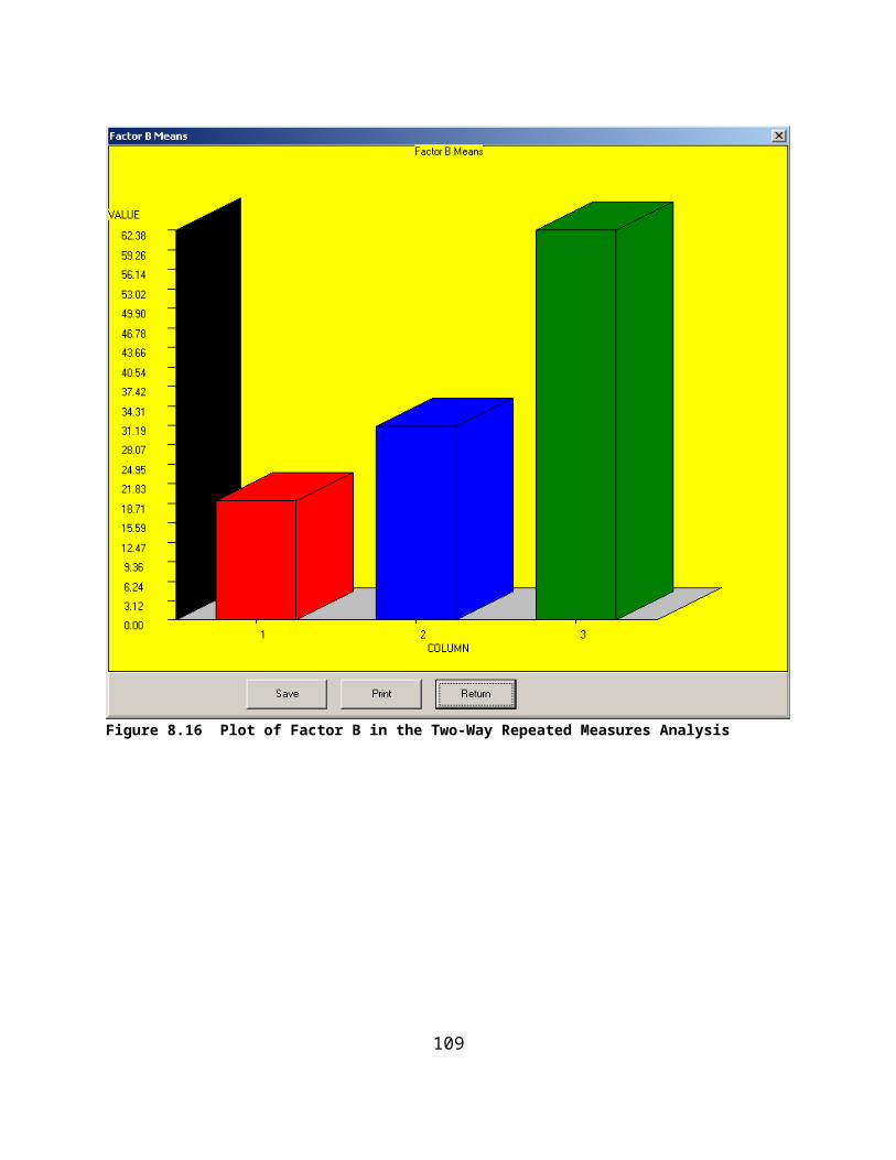
BLOCK 3
Cell means and totals-------------------------------------------------- Drug 1 2 3 Total-------------------------------------------------- Hospital 1 3.500 2.250 1.500 2.417 2 2.250 3.750 2.500 2.833 3 2.750 1.250 1.500 1.833 Total 2.833 2.417 1.833 4.074 --------------------------------------------------
Means for each variable
-------------------------------------------------- Hospital 1 2 3 Total-------------------------------------------------- 3.778 4.778 3.667 4.074 --------------------------------------------------
-------------------------------------------------- Drug 1 2 3 Total-------------------------------------------------- 5.361 4.778 2.083 4.074 --------------------------------------------------
-------------------------------------------------- Category 1 2 3 Total-------------------------------------------------- 4.056 5.806 2.361 4.074 --------------------------------------------------
-------------------------------------------------- Block 1 2 3 Total-------------------------------------------------- 4.500 4.222 3.500 4.074 --------------------------------------------------
Here, the main effect of factor D is partially confounded with the ABC interaction.
109

Analysis of Greco-Latin Squares
The specifications for the analysis are entered as:
Figure 8.24 Latin Square Design Form
The results are obtained as:
110

Greco-Latin Square Analysis (No Interactions)
-----------------------------------------------------------Source SS DF MS F Prob.>F-----------------------------------------------------------Factor A 64.889 2 32.444 9.733 0.001Factor B 64.889 2 32.444 9.733 0.001Latin Sqr. 24.889 2 12.444 3.733 0.037Greek Sqr. 22.222 2 11.111 3.333 0.051Residual - - - - -Within 90.000 27 3.333Total 266.889 35-----------------------------------------------------------
Experimental Design for Latin Square ------------------------------ B 1 2 3 ------------------------------ A 1 C1 C2 C3 2 C2 C3 C1 3 C3 C1 C2------------------------------
Experimental Design for Greek Square ------------------------------ B 1 2 3 ------------------------------ A 1 C1 C2 C3 2 C3 C1 C2 3 C2 C3 C1------------------------------
Cell means and totals-------------------------------------------------- B 1 2 3 Total-------------------------------------------------- A 1 4.000 6.000 7.000 5.667 2 6.000 12.000 8.000 8.667 3 7.000 8.000 10.000 8.333 Total 5.667 8.667 8.333 7.556 --------------------------------------------------
Means for each variable
-------------------------------------------------- A 1 2 3 Total-------------------------------------------------- 5.667 8.667 8.333 7.556 --------------------------------------------------
111

-------------------------------------------------- B 1 2 3 Total-------------------------------------------------- 5.667 8.667 8.333 7.556 --------------------------------------------------
-------------------------------------------------- Latin 1 2 3 Total-------------------------------------------------- 6.667 7.333 8.667 7.556 --------------------------------------------------
-------------------------------------------------- Greek 1 2 3 Total-------------------------------------------------- 8.667 7.000 7.000 7.556 --------------------------------------------------
Notice that in the case of 3 levels that the residual degrees of freedom are 0 hence no term is shown for the residual in this example. For more than 3 levels the test of the residuals provides a partial check on the assumptions of negligible interactions. The residual is sometimes combined with the within cell variance to provide an over-all estimate of variation due to experimental error.
112

Plan 5 Latin Square Design
The specifications for the analysis of the sample file “LatinPlan5.TAB” is shown below:
Figure 8.25 Latin Square Plan 5 Specifications Form
If you examine the sample file, you will notice that the subject Identification numbers (1,2,3,4) for the subjects in each group are the same even though the subjects in each group are different from group to group. The same ID is used in each group because they become “subscripts” for several arrays in the program. The results for our sample data are shown below:
Sums for ANOVA Analysis
Group (rows) times A Factor (columns) sums with 36 cases.
Variables 1 2 3 Total 1 14.000 19.000 18.000 51.000 2 15.000 18.000 16.000 49.000 3 14.000 21.000 18.000 53.000 Total 43.000 58.000 52.000 153.000
Group (rows) times B (cells Factor) sums with 36 cases.
113
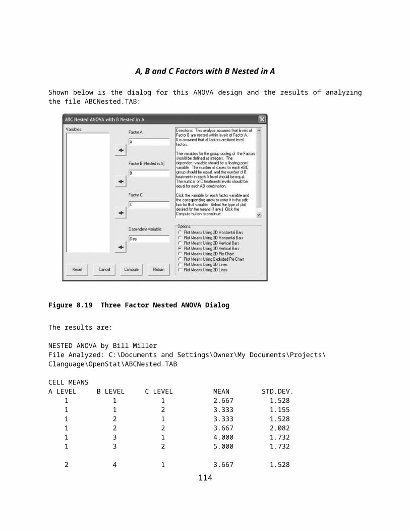
Variables 1 2 3 Total 1 19.000 18.000 14.000 51.000 2 15.000 18.000 16.000 49.000 3 18.000 14.000 21.000 53.000 Total 52.000 50.000 51.000 153.000
Groups (rows) times Subjects (columns) matrix with 36 cases.
Variables 1 2 3 4 Total 1 13.000 11.000 13.000 14.000 51.000 2 10.000 14.000 10.000 15.000 49.000 3 13.000 9.000 17.000 14.000 53.000 Total 36.000 34.000 40.000 43.000 153.000
Latin Squares Repeated Analysis Plan 5 (Partial Interactions)
-----------------------------------------------------------Source SS DF MS F Prob.>F-----------------------------------------------------------Betw.Subj. 20.083 11 Groups 0.667 2 0.333 0.155 0.859 Subj.w.g. 19.417 9 2.157
Within Sub 36.667 24 Factor A 9.500 2 4.750 3.310 0.060 Factor B 0.167 2 0.083 0.058 0.944 Factor AB 1.167 2 0.583 0.406 0.672 Error w. 25.833 18 1.435Total 56.750 35-----------------------------------------------------------
Experimental Design for Latin Square ------------------------------ A (Col) 1 2 3 ------------------------------Group (row) 1 B3 B1 B2 2 B1 B2 B3 3 B2 B3 B1------------------------------
Cell means and totals-------------------------------------------------- A (Col) 1 2 3 Total--------------------------------------------------Group (row) 1 3.500 4.750 4.500 4.250 2 3.750 4.500 4.000 4.083 3 3.500 5.250 4.500 4.417
114

Total 3.583 4.833 4.333 4.250 --------------------------------------------------
Means for each variable
-------------------------------------------------- A (Col) 1 2 3 Total-------------------------------------------------- 4.333 4.167 4.250 4.250 --------------------------------------------------
-------------------------------------------------- B (Cell) 1 2 3 Total-------------------------------------------------- 4.250 4.083 4.417 4.250 --------------------------------------------------
--------------------------------------------------Group (row) 1 2 3 Total-------------------------------------------------- 4.250 4.083 4.417 4.250 --------------------------------------------------
115

Plan 6 Latin Squares Design
LatinPlan6.TAB is the name of a sample file which you can analyze with the Plan 6 option of the Latin squares analysis procedure. Shown below is the specification form for the analysis of the data in that file:
Figure 8.26 Latin Square Plan 6 Specification
The results obtained when you click the OK button are shown below:
Latin Squares Repeated Analysis Plan 6
Sums for ANOVA Analysis
Group - C (rows) times A Factor (columns) sums with 36 cases.
Variables 1 2 3 Total 1 23.000 16.000 22.000 61.000 2 22.000 14.000 18.000 54.000 3 24.000 21.000 21.000 66.000 Total 69.000 51.000 61.000 181.000
116

Group - C (rows) times B (cells Factor) sums with 36 cases.
Variables 1 2 3 Total 1 16.000 22.000 23.000 61.000 2 22.000 14.000 18.000 54.000 3 21.000 24.000 21.000 66.000 Total 59.000 60.000 62.000 181.000
Group - C (rows) times Subjects (columns) matrix with 36 cases.
Variables 1 2 3 4 Total 1 16.000 14.000 13.000 18.000 61.000 2 12.000 13.000 14.000 15.000 54.000 3 18.000 19.000 11.000 18.000 66.000 Total 46.000 46.000 38.000 51.000 181.000
Latin Squares Repeated Analysis Plan 6
-----------------------------------------------------------Source SS DF MS F Prob.>F-----------------------------------------------------------Betw.Subj. 26.306 11 Factor C 6.056 2 3.028 1.346 0.308 Subj.w.g. 20.250 9 2.250
Within Sub 70.667 24 Factor A 13.556 2 6.778 2.259 0.133 Factor B 0.389 2 0.194 0.065 0.937 Residual 2.722 2 1.361 0.454 0.642 Error w. 54.000 18 3.000Total 96.972 35-----------------------------------------------------------
Experimental Design for Latin Square ------------------------------ A (Col) 1 2 3 ------------------------------ G C 1 1 B3 B1 B2 2 2 B1 B2 B3 3 3 B2 B3 B1------------------------------
117
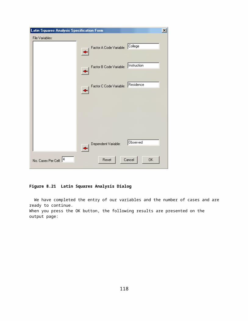
Cell means and totals-------------------------------------------------- A (Col) 1 2 3 Total-------------------------------------------------- Group+C 1 5.750 4.000 5.500 5.083 2 5.500 3.500 4.500 4.500 3 6.000 5.250 5.250 5.500 Total 5.750 4.250 5.083 5.028 --------------------------------------------------
Means for each variable
-------------------------------------------------- A (Col) 1 2 3 Total-------------------------------------------------- 4.917 5.000 5.167 5.028 --------------------------------------------------
-------------------------------------------------- B (Cell) 1 2 3 Total-------------------------------------------------- 5.083 4.500 5.500 5.028 --------------------------------------------------
-------------------------------------------------- Group+C 1 2 3 Total-------------------------------------------------- 5.083 4.500 5.500 5.028 --------------------------------------------------
118

Plan 7 for Latin Squares
Shown below is the specification for analysis of the sample data file labeled LatinPlan7.TAB and the results of the analysis:
Figure 8.27 Latin Squares Repeated Analysis Plan 7 Form
Sums for ANOVA Analysis
Group (rows) times A Factor (columns) sums with 36 cases.
Variables 1 2 3 Total 1 23.000 16.000 22.000 61.000 2 22.000 14.000 18.000 54.000 3 24.000 21.000 21.000 66.000 Total 69.000 51.000 61.000 181.000
Group (rows) times B (cells Factor) sums with 36 cases.
119

Variables 1 2 3 Total 1 23.000 16.000 22.000 61.000 2 18.000 22.000 14.000 54.000 3 21.000 21.000 24.000 66.000 Total 62.000 59.000 60.000 181.000
Group (rows) times C (cells Factor) sums with 36 cases.
Variables 1 2 3 Total 1 23.000 22.000 16.000 61.000 2 14.000 22.000 18.000 54.000 3 21.000 21.000 24.000 66.000 Total 58.000 65.000 58.000 181.000
Group (rows) times Subjects (columns) sums with 36 cases.
Variables 1 2 3 4 Total 1 16.000 14.000 13.000 18.000 61.000 2 12.000 13.000 14.000 15.000 54.000 3 18.000 19.000 11.000 18.000 66.000 Total 46.000 46.000 38.000 51.000 181.000
Latin Squares Repeated Analysis Plan 7 (superimposed squares)
-----------------------------------------------------------Source SS DF MS F Prob.>F-----------------------------------------------------------Betw.Subj. 26.306 11 Groups 6.056 2 3.028 1.346 0.308 Subj.w.g. 20.250 9 2.250
Within Sub 70.667 24 Factor A 13.556 2 6.778 2.259 0.133 Factor B 0.389 2 0.194 0.065 0.937 Factor C 2.722 2 1.361 0.454 0.642 residual - 0 - Error w. 54.000 18 3.000Total 96.972 35-----------------------------------------------------------
Experimental Design for Latin Square
120
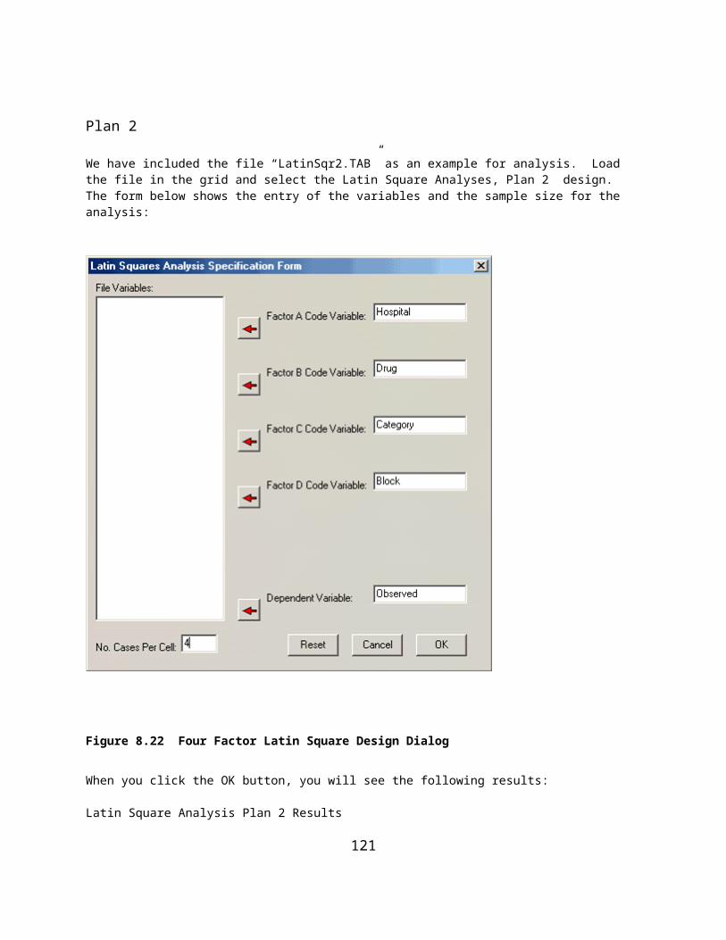
------------------------------ A (Col) 1 2 3 ------------------------------ Group
5. BC11 BC23 BC325. BC22 BC31 BC135. BC33 BC12 BC21
------------------------------
Cell means and totals-------------------------------------------------- A (Col) 1 2 3 Total-------------------------------------------------- Group 1 5.750 4.000 5.500 5.083 2 5.500 3.500 4.500 4.500 3 6.000 5.250 5.250 5.500 Total 5.750 4.250 5.083 5.028 --------------------------------------------------
Means for each variable
-------------------------------------------------- A (Col) 1 2 3 Total-------------------------------------------------- 5.750 4.250 5.083 5.028 --------------------------------------------------
-------------------------------------------------- B (Cell) 1 2 3 Total-------------------------------------------------- 5.167 4.917 5.000 5.028 --------------------------------------------------
-------------------------------------------------- C (Cell) 1 2 3 Total-------------------------------------------------- 4.833 5.417 4.833 5.028 --------------------------------------------------
-------------------------------------------------- Group 1 2 3 Total-------------------------------------------------- 5.083 4.500 5.500 5.028 --------------------------------------------------
121

Plan 9 Latin Squares
The sample data set labeled “LatinPlan9.TAB” is used for the following analysis. The specification form shown below has the variables entered for the analysis. When you click the OK button, the results obtained are as shown following the form.
Figure 8.28 Latin Squares Repeated Analysis Plan 9 Form
Sums for ANOVA Analysis
ABC matrix
C level 1 1 2 3 1 13.000 3.000 9.000 2 6.000 9.000 3.000 3 10.000 14.000 15.000
C level 2 1 2 3 1 18.000 14.000 18.000 2 19.000 24.000 20.000 3 8.000 11.000 10.000
122

C level 3 1 2 3 1 17.000 12.000 20.000 2 14.000 13.000 9.000 3 15.000 12.000 17.000
AB sums with 18 cases.
Variables 1 2 3 Total 1 48.000 29.000 47.000 124.000 2 39.000 46.000 32.000 117.000 3 33.000 37.000 42.000 112.000 Total 120.000 112.000 121.000 353.000
AC sums with 18 cases.
Variables 1 2 3 Total 1 25.000 50.000 49.000 124.000 2 18.000 63.000 36.000 117.000 3 39.000 29.000 44.000 112.000 Total 82.000 142.000 129.000 353.000
BC sums with 18 cases.
Variables 1 2 3 Total 1 29.000 45.000 46.000 120.000 2 26.000 49.000 37.000 112.000 3 27.000 48.000 46.000 121.000 Total 82.000 142.000 129.000 353.000
RC sums with 18 cases.
Variables 1 2 3 Total 1 16.000 42.000 36.000 94.000
123

2 37.000 52.000 47.000 136.000 3 29.000 48.000 46.000 123.000 Total 82.000 142.000 129.000 353.000
Group totals with 18 valid cases.
Variables 1 2 3 4 5 16.000 37.000 29.000 42.000 52.000
Variables 6 7 8 9 Total 48.000 36.000 47.000 46.000 353.000
Subjects sums with 18 valid cases.
Variables 1 2 3 4 5 7.000 9.000 14.000 28.000 15.000
Variables 6 7 8 9 10 21.000 16.000 21.000 22.000 30.000
Variables 11 12 13 14 15 28.000 19.000 10.000 19.000 23.000
Variables 16 17 18 Total 25.000 28.000 18.000 0.000
Latin Squares Repeated Analysis Plan 9
-----------------------------------------------------------Source SS DF MS F Prob.>F-----------------------------------------------------------Betw.Subj. 267.426 17 Factor C 110.704 2 55.352 5.058 0.034 Rows 51.370 2 25.685 2.347 0.151 C x row 6.852 4 1.713 0.157 0.955 Subj.w.g. 98.500 9 10.944
Within Sub 236.000 36 Factor A 4.037 2 2.019 0.626 0.546 Factor B 2.704 2 1.352 0.420 0.664 Factor AC 146.519 4 36.630 11.368 0.000 Factor BC 8.519 4 2.130 0.661 0.627 AB prime 7.148 2 3.574 1.109 0.351 ABC prime 9.074 4 2.269 0.704 0.599
124

Error w. 58.000 18 3.222
Total 503.426 53-----------------------------------------------------------
Experimental Design for Latin Square
------------------------------ FactorA 1 2 3 ------------------------------ Group 1 B2 B3 B1 2 B1 B2 B3 3 B3 B1 B2 4 B2 B3 B1 5 B1 B2 B3 6 B3 B1 B2 7 B2 B3 B1 8 B1 B2 B3 9 B3 B1 B2------------------------------
Latin Squares Repeated Analysis Plan 9
Means for ANOVA Analysis
ABC matrix
C level 1 1 2 3 1 6.500 1.500 4.500 2 3.000 4.500 1.500 3 5.000 7.000 7.500
C level 2 1 2 3 1 9.000 7.000 9.000 2 9.500 12.000 10.000 3 4.000 5.500 5.000
C level 3 1 2 3 1 8.500 6.000 10.000 2 7.000 6.500 4.500 3 7.500 6.000 8.500
AB Means with 54 cases.
125

Variables 1 2 3 4 1 8.000 4.833 7.833 6.889 2 6.500 7.667 5.333 6.500 3 5.500 6.167 7.000 6.222 Total 6.667 6.222 6.722 6.537
AC Means with 54 cases.
Variables 1 2 3 4 1 4.167 8.333 8.167 6.889 2 3.000 10.500 6.000 6.500 3 6.500 4.833 7.333 6.222 Total 4.556 7.889 7.167 6.537
BC Means with 54 cases.
Variables 1 2 3 4 1 4.833 7.500 7.667 6.667 2 4.333 8.167 6.167 6.222 3 4.500 8.000 7.667 6.722 Total 4.556 7.889 7.167 6.537
RC Means with 54 cases.
Variables 1 2 3 4 1 2.667 7.000 6.000 5.222 2 6.167 8.667 7.833 7.556 3 4.833 8.000 7.667 6.833 Total 4.556 7.889 7.167 6.537
Group Means with 54 valid cases.
Variables 1 2 3 4 5
126

2.667 6.167 4.833 7.000 8.667
Variables 6 7 8 9 Total 8.000 6.000 7.833 7.667 6.537
Subjects Means with 54 valid cases.
Variables 1 2 3 4 5 3.500 4.500 7.000 14.000 7.500
Variables 6 7 8 9 10 10.500 8.000 10.500 11.000 15.000
Variables 11 12 13 14 15 14.000 9.500 5.000 9.500 11.500
Variables 16 17 18 Total 12.500 14.000 9.000 6.537
127
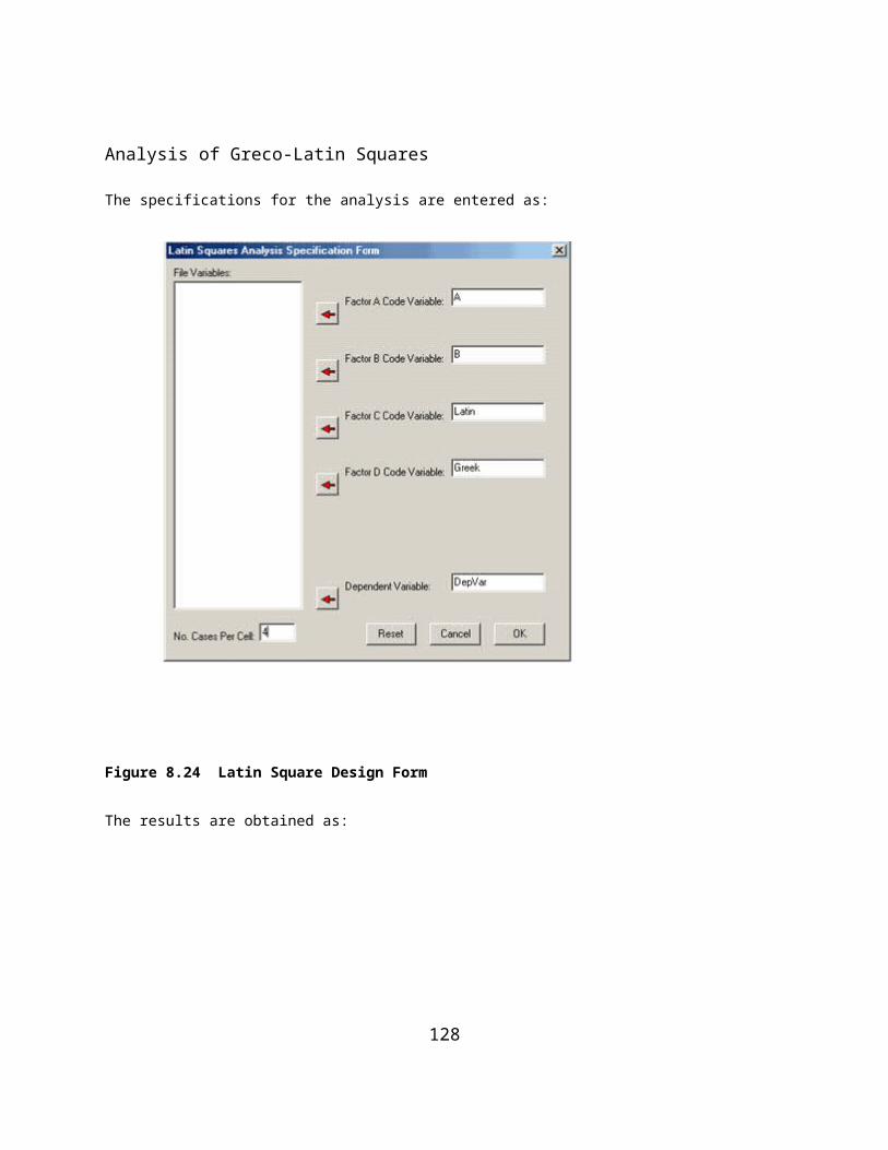
2 or 3 Way Fixed ANOVA with 1 case per cell
There may be an occasion where you have collected data with a single observation within two or three factor combinations. In this case one cannot obtain an estimate of the variance within a single cell of the two or three factor design and thus an estimate of the mean squared error term typically used in a 2 or 3 way ANOVA. The estimate of error must be made using all cell values. To demonstrate, the following data are analyzed:
CASES FOR FILE C:\Users\wgmiller\Projects\Data\OneCase2Way.TEX
0 Row Col Dep CASE 1 1 1 1.000 CASE 2 1 2 2.000 CASE 3 1 3 3.000 CASE 4 2 1 3.000 CASE 5 2 2 5.000 CASE 6 2 3 9.000
The dialog for this procedure and the resulting output are shown below:
Figure 8.29 Dialog for 2 or 3 Way ANOVA with One Case Per Cell
Two Way Analysis of Variance
Variable analyzed: Dep
Factor A (rows) variable: RowFactor B (columns) variable: Col
SOURCE D.F. SS MS F PROB.> F Omega Squared
Among Rows 1 20.167 20.167 9.308 0.093 0.419
128

Among Columns 2 16.333 8.167 3.769 0.210 0.279Residual 2 4.333 2.167 NonAdditivity 1 4.252 4.252 52.083 0.088 Balance 1 0.082 0.082Total 5 40.833 8.167
Omega squared for combined effects = 0.698
Descriptive Statistics
GROUP Row Col. N MEAN VARIANCE STD.DEV.Cell 1 1 1 1.000 0.000 0.000Cell 1 2 1 2.000 0.000 0.000Cell 1 3 1 3.000 0.000 0.000Cell 2 1 1 3.000 0.000 0.000Cell 2 2 1 5.000 0.000 0.000Cell 2 3 1 9.000 0.000 0.000Row 1 3 2.000 1.000 1.000Row 2 3 5.667 9.333 3.055Col 1 2 2.000 2.000 1.414Col 2 2 3.500 4.500 2.121Col 3 2 6.000 18.000 4.243TOTAL 6 3.833 8.167 2.858
Figure 8.30 One Case ANOVA Plot for Factor 1
129

Figure 8.31 Factor 2 Plot for One Case ANOVA
Figure 8.32 Interaction Plot of Two Factors for One Case ANOVA
130

Two Within Subjects ANOVA
You may have observed the same subjects under two “treatment” factors. As an example, you might have observed subject responses on a visual acuity test before and after consuming an alcoholic beverage. In this case we do not have a “between subjects” analysis but rather a “repeated measures” analysis under two conditions. As an example, we will analyze data from a file labeled “”. The data, the dialog and the results are shown below:
Figure 8.33 Dialog for Two Within Subjects ANOVA
131

Figure 8.34 Factor One Plot for Two Within Subjects ANOVA
Figure 8.35 Factor Two Plot for Two Within Subjects ANOVA
132

Figure 8.36 Two Way Interaction for Two Within Subjects ANOVA
-------------------------------------------------------------------SOURCE DF SS MS F Prob.>F-------------------------------------------------------------------Factor A 1 204.167 204.167 9.853 0.052Factor B 2 8039.083 4019.542 24.994 0.001Subjects 3 1302.833 434.278A x B Interaction 2 46.583 23.292 0.803 0.491A x S Interaction 3 62.167 20.722B x S Interaction 6 964.917 160.819A x B x S Inter. 6 174.083 29.01-------------------------------------------------------------------Total 23 10793.833-------------------------------------------------------------------Group 1 : Mean for cell A 1 and B 1 = 17.250Group 2 : Mean for cell A 1 and B 2 = 26.000Group 3 : Mean for cell A 1 and B 3 = 60.250Group 4 : Mean for cell A 2 and B 1 = 20.750Group 5 : Mean for cell A 2 and B 2 = 35.750Group 6 : Mean for cell A 2 and B 3 = 64.500
Means for Factor AGroup 1 Mean = 34.500Group 2 Mean = 40.333
Means for Factor BGroup 1 Mean = 19.000Group 2 Mean = 30.875Group 3 Mean = 62.375
133

IX. Multivariate Procedures
Analysis of Variance Using Multiple Regression Methods
An Example of an Analysis of Covariance
We will demonstrate the analysis of covariance procedure using multiple regression by loading the file labeled “Ancova2.tab” . In this file we have a treatment group code for four groups, a dependent variable (X) and two covariates (Y and Z.) The procedure is started by selection the “Analysis of Covariance by Regression” option in the Comparisons sub-menu under the Statistics menu. Shown below is the completed specification form for our analysis:
Figure 9.1 Analysis of Covariance Dialog
When we click the Compute button, the following results are obtained:
ANALYSIS OF COVARIANCE USING MULTIPLE REGRESSION
File Analyzed: C:\Projects\Delphi\OpenStat\Ancova2.txt
Model for Testing Assumption of Zero Interactions with Covariates
MEANS with 40 valid cases.
134

Variables X Z A1 A2 A3 7.125 14.675 0.000 0.000 0.000
Variables XxA1 XxA2 XxA3 ZxA1 ZxA2 0.125 0.025 0.075 -0.400 -0.125
Variables ZxA3 Y -0.200 17.550
VARIANCES with 40 valid cases.
Variables X Z A1 A2 A3 4.163 13.866 0.513 0.513 0.513
Variables XxA1 XxA2 XxA3 ZxA1 ZxA2 28.010 27.102 27.712 116.759 125.035
Variables ZxA3 Y 124.113 8.254
STD. DEV.S with 40 valid cases.
Variables X Z A1 A2 A3 2.040 3.724 0.716 0.716 0.716
Variables XxA1 XxA2 XxA3 ZxA1 ZxA2 5.292 5.206 5.264 10.806 11.182
Variables ZxA3 Y 11.141 2.873 R R2 F Prob.>F DF1 DF2
0.842 0.709 6.188 0.000 11 28Adjusted R Squared = 0.594
Std. Error of Estimate = 1.830
Variable Beta B Std.Error t Prob.>t X 0.599 0.843 0.239 3.531 0.001 Z 0.123 0.095 0.138 0.686 0.498 A1 -0.518 -2.077 2.381 -0.872 0.391 A2 0.151 0.606 2.513 0.241 0.811 A3 0.301 1.209 2.190 0.552 0.585 XxA1 -1.159 -0.629 0.523 -1.203 0.239 XxA2 0.714 0.394 0.423 0.932 0.359 XxA3 0.374 0.204 0.334 0.611 0.546 ZxA1 1.278 0.340 0.283 1.200 0.240 ZxA2 -0.803 -0.206 0.284 -0.727 0.473 ZxA3 -0.353 -0.091 0.187 -0.486 0.631
Constant = 10.300
135

Analysis of Variance for the Model to Test Regression Homogeneity SOURCE Deg.F. SS MS F Prob>F Explained 11 228.08 20.73 6.188 0.0000 Error 28 93.82 3.35 Total 39 321.90
Model for Analysis of Covariance
MEANS with 40 valid cases.
Variables X Z A1 A2 A3 7.125 14.675 0.000 0.000 0.000
Variables Y 17.550
VARIANCES with 40 valid cases.
Variables X Z A1 A2 A3 4.163 13.866 0.513 0.513 0.513
Variables Y 8.254
STD. DEV.S with 40 valid cases.
Variables X Z A1 A2 A3 2.040 3.724 0.716 0.716 0.716
Variables Y 2.873 R R2 F Prob.>F DF1 DF2
0.830 0.689 15.087 0.000 5 34Adjusted R Squared = 0.644
Std. Error of Estimate = 1.715
Variable Beta B Std.Error t Prob.>t X 0.677 0.954 0.184 5.172 0.000 Z 0.063 0.048 0.102 0.475 0.638 A1 -0.491 -1.970 0.487 -4.044 0.000 A2 0.114 0.458 0.472 0.972 0.338 A3 0.369 1.482 0.470 3.153 0.003
Constant = 10.046
Test for Homogeneity of Group Regression Coefficients
136

Change in R2 = 0.0192. F = 0.308 Prob.> F = 0.9275 with d.f. 6 and 28
Analysis of Variance for the ANCOVA Model SOURCE Deg.F. SS MS F Prob>F Explained 5 221.89 44.38 15.087 0.0000 Error 34 100.01 2.94 Total 39 321.90
Intercepts for Each Group Regression Equation for Variable: Group
Intercepts with 40 valid cases.
Variables Group 1 Group 2 Group 3 Group 4 8.076 10.505 11.528 10.076
Adjusted Group Means for Group Variables Group
Means with 40 valid cases.
Variables Group 1 Group 2 Group 3 Group 4 15.580 18.008 19.032 17.579
Multiple Comparisons Among Group Means
Comparison of Group 1 with Group 2F = 9.549, probability = 0.004 with degrees of freedom 1 and 34Comparison of Group 1 with Group 3F = 19.849, probability = 0.000 with degrees of freedom 1 and 34Comparison of Group 1 with Group 4F = 1.546, probability = 0.222 with degrees of freedom 1 and 34Comparison of Group 2 with Group 3F = 1.770, probability = 0.192 with degrees of freedom 1 and 34Comparison of Group 2 with Group 4F = 3.455, probability = 0.072 with degrees of freedom 1 and 34Comparison of Group 3 with Group 4F = 9.973, probability = 0.003 with degrees of freedom 1 and 34
Test for Each Source of Variance SOURCE Deg.F. SS MS F Prob>F A 3 60.98 20.33 6.911 0.0009Covariates 2 160.91 80.45 27.352 0.0000 Error 34 100.01 2.94 Total 39 321.90
The results reported above begin with a regression model that includes group coding for the four groups (A1, A2 and A3) and again note that the fourth group is automatically identified by members NOT being in one of
137
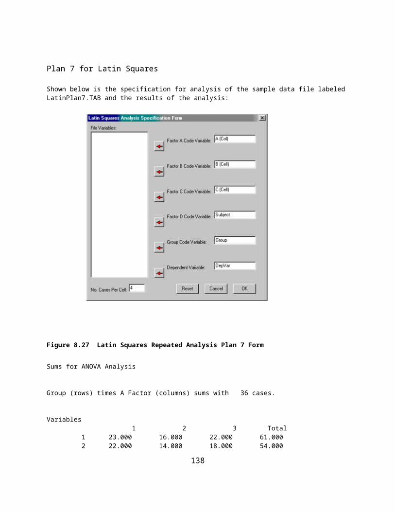
the first three groups. This model also contains the covariates X and Z as well as the cross-products of group membership and covariates. By comparing this model with the second model created (one which leaves out the cross-products of groups and covariates) we can assess the degree to which the assumptions of homogeneity of covariance among the groups is met. In this particular example, the change in the R2 from the full model to the restricted model was quite small (0.0192) and we conclude that the assumption of homogeneity of covariance is reasonable. The analysis of variance model for the restricted model indicates that the X covariate is probably contributing significantly to the explained variance of the dependent variable Y. The tests for each source of variance at the end of the report confirms that not only are the covariates related to Y but that the group effects are also significant. The comparisons of the group means following adjustment for the covariate effects indicate that group 1 differs from groups 2 and 3 and that group 3 appears to differ from group 4.
138

Sums of Squares by Regression
The General Linear Model (GLM) procedure is an analysis procedure that encompasses a variety of analyses. It may incorporate multiple linear regression as well as canonical correlation analysis as methods for analyzing the user's data. In some commercial statistics packages the GLM method also incorporates non-linear analyses, maximum-likelihood procedures and a variety of tests not found in the OPENSTAT version of this model. The version in OpenStat is currently limited to a single dependent variable (continuous measure.) You should complete analyses with multiple dependent variables with the Canonical Correlation procedure.
One can complete a variety of analyses of variance with the GLM procedure including multiple factor ANOVA and repeated and mixed model ANOVAs.
The output of the GLM can be somewhat voluminous in that the effects of treatment variables and covariates are analyzed individually by comparing regression models with and without those variables. Several examples are explored below.
When you elect the Sum of Squares by Regression procedure from either the Regression options or the Multivariate options of the Analyses menu, you will see the form shown below. In our first example we will select a data file for completion of a repeated measures analysis of variance that involves two between-groups factors and one within groups factor (the SSRegs2.TAB file.) The data file contains codes for Factor A treatment levels, Factor B treatment levels, the replications factor (Factor C levels), and a code for each subject. In our analysis we will define the two-way and the one three-way interactions that we wish to include in our model. We should then be able to compare our results with the Repeated Measures ANOVA procedure applied to the same data in the file labeled ABRData.TAB (and hopefully see the same results!)
Figure 9.2 Sum of Squares by Regression
139

SUMS OF SQUARES AND MEAN SQUARES BY REGRESSIONTYPE III SS - R2 = Full Model - Restricted Model
VARIABLE SUM OF SQUARES D.F.
Row1 10.083 1 Col1 8.333 1 Rep1 150.000 1 Rep2 312.500 1 Rep3 529.000 1 C1R1 80.083 1 R1R1 0.167 1 R2R1 2.000 1 R3R1 6.250 1 R1C1 4.167 1 R2C1 0.889 1 R3C1 7.111 1ERROR 147.417 35TOTAL 1258.000 47
TOTAL EFFECTS SUMMARY-----------------------------------------------------------SOURCE SS D.F. MS----------------------------------------------------------- Row 10.083 1 10.083 Col 8.333 1 8.333 Rep 991.500 3 330.500 Row*Col 80.083 1 80.083 Row*Rep 8.417 3 2.806 Col*Rep 12.167 3 4.056-----------------------------------------------------------
-----------------------------------------------------------SOURCE SS D.F. MS-----------------------------------------------------------BETWEEN SUBJECTS 181.000 11 Row 10.083 1 10.083 Col 8.333 1 8.333 Row*Col 80.083 1 80.083ERROR BETWEEN 82.500 8 10.312
-----------------------------------------------------------WITHIN SUBJECTS 1077.000 36 Rep 991.500 3 330.500 Row*Rep 8.417 3 2.806 Col*Rep 12.167 3 4.056ERROR WITHIN 64.917 27 2.404
-----------------------------------------------------------TOTAL 1258.000-----------------------------------------------------------
140

You can compare the results above with an analysis completed with the Repeated Measures procedure.
As a second example, we will complete and analysis of covariance on data that contains three treatment factors and two covariates. The file analyzed is labeled ANCOVA3.TAB. Shown below is the dialog for the analysis followed by the output. You can compare this output with the output obtained by analyzing the same data file with the Analysis of Covariance procedure.
Figure 9.3 Example 2 of Sum of Squares by Regression
SUMS OF SQUARES AND MEAN SQUARES BY REGRESSIONTYPE III SS - R2 = Full Model - Restricted Model
VARIABLE SUM OF SQUARES D.F.
Cov1 1.275 1 Cov2 0.783 1 Row1 25.982 1 Col1 71.953 1 Slice1 13.323 1 Slice2 0.334 1 C1R1 21.240 1
141
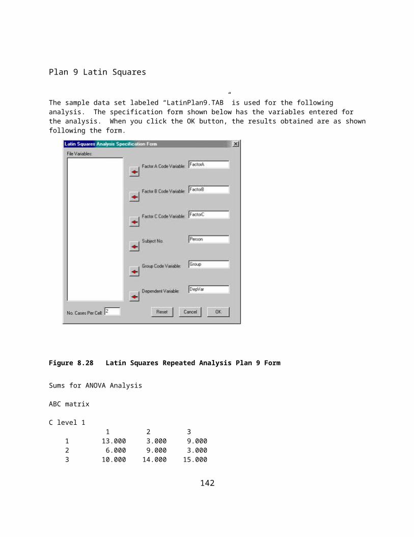
S1R1 11.807 1 S2R1 0.138 1 S1C1 13.133 1 S2C1 0.822 1 S1C1R1 0.081 1 S2C1R1 47.203 1ERROR 46.198 58TOTAL 269.500 71
TOTAL EFFECTS SUMMARY-----------------------------------------------------------SOURCE SS D.F. MS----------------------------------------------------------- Cov1 1.275 1 1.275 Cov2 0.783 1 0.783 Row 25.982 1 25.982 Col 71.953 1 71.953 Slice 13.874 2 6.937 Row*Col 21.240 1 21.240 Row*Slice 11.893 2 5.947 Col*Slice 14.204 2 7.102 Row*Col*Slice 47.247 2 23.624-----------------------------------------------------------
-----------------------------------------------------------SOURCE SS D.F. MS-----------------------------------------------------------BETWEEN SUBJECTS 208.452 13 Covariates 2.058 2 1.029 Row 25.982 1 25.982 Col 71.953 1 71.953 Slice 13.874 2 6.937 Row*Col 21.240 1 21.240 Row*Slice 11.893 2 5.947 Col*Slice 14.204 2 7.102 Row*Col*Slice 47.247 2 23.624ERROR BETWEEN 46.198 58 0.797
-----------------------------------------------------------
-----------------------------------------------------------TOTAL 269.500 71-----------------------------------------------------------
==================================================================
142

The General Linear Model
We have seen in the above discussion that the multiple regression method may be used to complete an analysis of variance for a single dependent variable. The model for multiple regression is:
where the jth B value is a coefficient multiplied times the jth independent predictor score, Y is the observed dependent score and e is the error (difference between the observed and the value predicted for Y using the sum of weighted independent scores.)
In some research it is desirable to determine the relationship between multiple dependent variables and multiple independent variables. Of course, one could complete a multiple regression analysis for each dependent variable but this would ignore the possible relationships among the dependent variables themselves. For example, a teacher might be interested in the relationship between the sub-scores on a standardized achievement test (independent variables) and the final examination results for several different courses (dependent variables.) Each of the final examination scores could be predicted by the sub-scores in separate analyses but most likely the interest is in knowing how well the sub-scores account for the combined variance of the achievement scores. By assigning weights to each of the dependent variables as well as the independent variables in such a way that the composite dependent score is maximally related to the composite independent score we can quantify the relationship between the two composite scores. We note that the squared product-moment correlation coefficient reflects the proportion of variance of a dependent variable predicted by the independent variable.
We can express the model for the general linear model as:
where Y is an n (the number of subjects) by m (the number of dependent variables) matrix of dependent variable values, M is a m by s (number of coefficient sets), X is a n by k (the number of independent variables) matrix, B is a k by s matrix of coefficients and E is a vector of errors for the n subjects.
143

Using OpenStat to Obtain Canonical Correlations
You can use the OpenStat package to obtain canonical correlations for a wide variety of applications. In production of bread, for example, a number of “dependent” quality variables may exist such as the average size of air bubbles in a slice, the density of a slice, the thickness of the crust, etc. Similarly, there are a number of “independent” variables which may be related to the dependent variables with examples being minutes of baking, temperature of baking, humidity in the oven, barometric pressure, time and temperature during rising of the dough, etc. The relationship between these two sets of variables might identify the “key” variables to control for maximizing the quality of the product.
To demonstrate use of OpenStat to obtain canonical correlations we will use the file labeled "cansas.txt" as an example. We will click on the Canonical Correlation option under the Correlation sub-menu of the Statistics menu. In the Figure below we show the form which appears and the data entered to initiate the analysis:
Figure 9.4 Canonical Correlation Analysis Form
We obtain the results as shown below:
CANONICAL CORRELATION ANALYSIS
Right Inverse x Right-Left Matrix with 20 valid cases.
Variables weight waist pulse chins -0.102 -0.226 0.001 situps -0.552 -0.788 0.365 jumps 0.193 0.448 -0.210
144

Left Inverse x Left-Right Matrix with 20 valid cases.
Variables chins situps jumps weight 0.368 0.287 -0.259 waist -0.882 -0.890 0.015 pulse -0.026 0.016 -0.055
Canonical Function with 20 valid cases.
Variables Var. 1 Var. 2 Var. 3 Var. 1 0.162 0.172 0.023 Var. 2 0.482 0.549 0.111 Var. 3 -0.318 -0.346 -0.032
Trace of the matrix:= 0.6785Percent of trace extracted: 100.0000
Canonical R Root % Trace Chi-Sqr D.F. Prob. 2 0.795608 0.633 93.295 16.255 9 0.062 3 0.200556 0.040 5.928 0.718 4 0.949 4 0.072570 0.005 0.776 0.082 1 0.775
Overall Tests of Significance: Statistic Approx. Stat. Value D.F. Prob.>ValueWilk's Lambda Chi-Squared 17.3037 9 0.0442Hotelling-Lawley Trace F-Test 2.4938 9 38 0.0238Pillai Trace F-Test 1.5587 9 48 0.1551Roys Largest Root F-Test 10.9233 3 19 0.0002
Eigenvectors with 20 valid cases.
Variables Var. 1 Var. 2 Var. 3 Var. 1 0.210 -0.066 0.051 Var. 2 0.635 0.022 -0.049 Var. 3 -0.431 0.188 0.017
Standardized Right Side Weights with 20 valid cases.
Variables Var. 1 Var. 2 Var. 3
145

weight 0.775 -1.884 0.191 waist -1.579 1.181 -0.506 pulse 0.059 -0.231 -1.051
Standardized Left Side Weights with 20 valid cases.
Variables Var. 1 Var. 2 Var. 3 chins 0.349 -0.376 1.297 situps 1.054 0.123 -1.237 jumps -0.716 1.062 0.419
Standardized Right Side Weights with 20 valid cases.
Variables Var. 1 Var. 2 Var. 3 weight 0.775 -1.884 0.191 waist -1.579 1.181 -0.506 pulse 0.059 -0.231 -1.051
Raw Right Side Weights with 20 valid cases.
Variables Var. 1 Var. 2 Var. 3 weight 0.031 -0.076 0.008 waist -0.493 0.369 -0.158 pulse 0.008 -0.032 -0.146
Raw Left Side Weights with 20 valid cases.
Variables Var. 1 Var. 2 Var. 3 chins 0.066 -0.071 0.245 situps 0.017 0.002 -0.020 jumps -0.014 0.021 0.008
Right Side Correlations with Function with 20 valid cases.
Variables
146

Var. 1 Var. 2 Var. 3 weight -0.621 -0.772 0.135 waist -0.925 -0.378 0.031 pulse 0.333 0.041 -0.942
Left Side Correlations with Function with 20 valid cases.
Variables Var. 1 Var. 2 Var. 3 chins 0.728 0.237 0.644 situps 0.818 0.573 -0.054 jumps 0.162 0.959 0.234
Redundancy Analysis for Right Side Variables
Variance Prop. Redundancy 1 0.45080 0.28535 2 0.24698 0.00993 3 0.30222 0.00159
Redundancy Analysis for Left Side Variables Variance Prop. Redundancy 1 0.40814 0.25835 2 0.43449 0.01748 3 0.15737 0.00083
147

Binary Logistic Regression
When this analysis is selected from the menu, the form below is used to select the dependent and independent variables:
Figure 9.5 Logistic Regression Form
Output for the example analysis specified above is shown below:
Logistic Regression Adapted from John C. PezzulloJava program at http://members.aol.com/johnp71/logistic.html
Descriptive Statistics6 cases have Y=0; 4 cases have Y=1.Variable Label Average Std.Dev. 1 Var1 5.5000 2.8723
2 Var2 5.5000 2.8723
Iteration History-2 Log Likelihood = 13.4602 (Null Model)-2 Log Likelihood = 8.7491 -2 Log Likelihood = 8.3557
148

-2 Log Likelihood = 8.3302 -2 Log Likelihood = 8.3300 -2 Log Likelihood = 8.3300 Converged
Overall Model Fit... Chi Square = 5.1302 with df = 2 and prob. = 0.0769
Coefficients and Standard Errors...Variable Label Coeff. StdErr p 1 Var1 0.3498 0.6737 0.6036
2 Var2 0.3628 0.6801 0.5937Intercept -4.6669
Odds Ratios and 95% Confidence Intervals...Variable O.R. Low -- High Var1 1.4187 0.3788 5.3135 Var2 1.4373 0.3790 5.4506
X X Y Prob 1.0000 2.0000 0 0.0268 2.0000 1.0000 0 0.0265 3.0000 5.0000 0 0.1414 4.0000 3.0000 0 0.1016
5.0000 4.0000 1 0.1874 6.0000 7.0000 0 0.4929 7.0000 8.0000 1 0.6646 8.0000 6.0000 0 0.5764 9.0000 10.0000 1 0.8918 10.0000 9.0000 1 0.8905
149

Cox Proportional Hazards Survival Regression
The specification form for this analysis is shown below with variables entered for a sample file:
Figure 9.6 Cox Proportional Hazards Survival Regression Form
Results for the above sample are as follows:
Cox Proportional Hazards Survival Regression Adapted from John C. Pezzullo's Java program at http://members.aol.com/johnp71/prophaz.html
Descriptive StatisticsVariable Label Average Std.Dev. 1 VAR1 51.1818 10.9778
Iteration History...-2 Log Likelihood = 11.4076 (Null Model)
-2 Log Likelihood = 6.2582-2 Log Likelihood = 4.5390
150

-2 Log Likelihood = 4.1093-2 Log Likelihood = 4.0524-2 Log Likelihood = 4.0505-2 Log Likelihood = 4.0505Converged
Overall Model Fit...Chi Square = 7.3570 with d.f. 1 and probability = 0.0067
Coefficients, Std Errs, Signif, and Confidence Intervals
Var Coeff. StdErr p Lo95% Hi95% VAR1 0.3770 0.2542 0.1379 -0.1211 0.8752
Risk Ratios and Confidence Intervals
Variable Risk Ratio Lo95% Hi95% VAR1 1.4580 0.8859 2.3993
Baseline Survivor Function (at predictor means)... 2.0000 0.9979 7.0000 0.9820 9.0000 0.9525 10.0000 0.8310
151
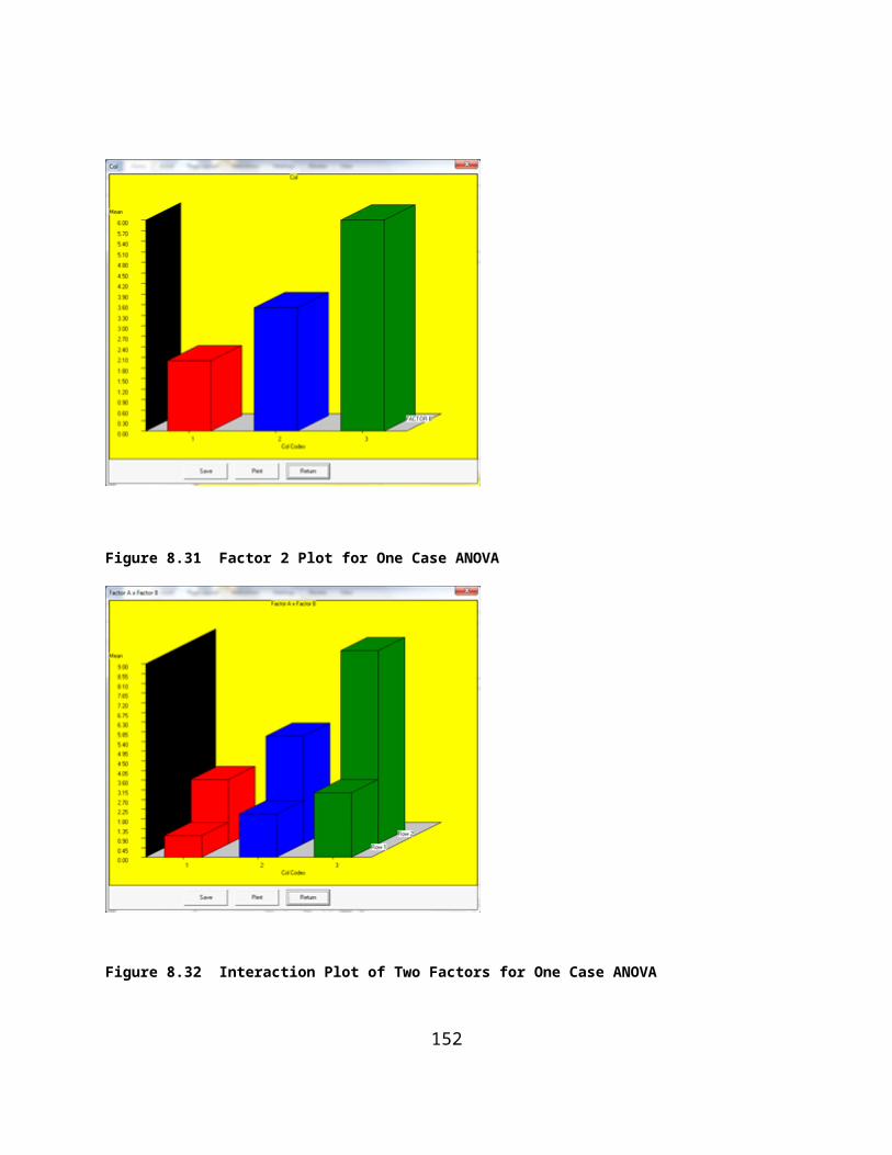
Weighted Least-Squares Regression
Shown below is the dialog box for the Weighted Least Squares Analysis and an analysis of the cansas.tab data file.
Figure 9.7 Weighted Least Squares Regression
OLS REGRESSION RESULTS
Means
Variables weight waist pulse chins situps jumps
178.600 35.400 56.100 9.450 145.550 70.300
Standard Deviations
Variables weight waist pulse chins situps
152

jumps
24.691 3.202 7.210 5.286 62.567 51.277
No. of valid cases = 20
CORRELATION MATRIX
VARIABLE weight waist pulse chins situps jumps weight 1.000 0.870 -0.366 -0.390 -0.493 -0.226 waist 0.870 1.000 -0.353 -0.552 -0.646 -0.191 pulse -0.366 -0.353 1.000 0.151 0.225 0.035 chins -0.390 -0.552 0.151 1.000 0.696 0.496 situps -0.493 -0.646 0.225 0.696 1.000 0.669 jumps -0.226 -0.191 0.035 0.496 0.669 1.000
Dependent variable: jumps
Variable Beta B Std.Err. t Prob.>t VIF TOL weight -0.588 -1.221 0.704 -1.734 0.105 4.424 0.226 waist 0.982 15.718 6.246 2.517 0.025 5.857 0.171 pulse -0.064 -0.453 1.236 -0.366 0.720 1.164 0.859 chins 0.201 1.947 2.243 0.868 0.400 2.059 0.486 situps 0.888 0.728 0.205 3.546 0.003 2.413 0.414 Intercept 0.000 -366.967 183.214 -2.003 0.065
SOURCE DF SS MS F Prob.>FRegression 5 31793.741 6358.748 4.901 0.0084Residual 14 18164.459 1297.461Total 19 49958.200
R2 = 0.6364, F = 4.90, D.F. = 5 14, Prob>F = 0.0084Adjusted R2 = 0.5066
Standard Error of Estimate = 36.02
REGRESSION OF SQUARED RESIDUALS ON INDEPENDENT VARIABLES
Means
Variables weight waist pulse chins situps ResidSqr
178.600 35.400 56.100 9.450 145.550 908.196
153

Standard Deviations
Variables weight waist pulse chins situps ResidSqr
24.691 3.202 7.210 5.286 62.567 2086.828
No. of valid cases = 20
CORRELATION MATRIX
VARIABLE weight waist pulse chins situps ResidSqr weight 1.000 0.870 -0.366 -0.390 -0.493 -0.297 waist 0.870 1.000 -0.353 -0.552 -0.646 -0.211 pulse -0.366 -0.353 1.000 0.151 0.225 -0.049 chins -0.390 -0.552 0.151 1.000 0.696 0.441 situps -0.493 -0.646 0.225 0.696 1.000 0.478 ResidSqr -0.297 -0.211 -0.049 0.441 0.478 1.000
Dependent variable: ResidSqr
Variable Beta B Std.Err. t Prob.>t VIF TOL weight -0.768 -64.916 36.077 -1.799 0.094 4.424 0.226 waist 0.887 578.259 320.075 1.807 0.092 5.857 0.171 pulse -0.175 -50.564 63.367 -0.798 0.438 1.164 0.859 chins 0.316 124.826 114.955 1.086 0.296 2.059 0.486 situps 0.491 16.375 10.515 1.557 0.142 2.413 0.414 Intercept 0.000 -8694.402 9389.303 -0.926 0.370
SOURCE DF SS MS F Prob.>FRegression 5 35036253.363 7007250.673 2.056 0.1323Residual 14 47705927.542 3407566.253Total 19 82742180.905
R2 = 0.4234, F = 2.06, D.F. = 5 14, Prob>F = 0.1323Adjusted R2 = 0.2175
Standard Error of Estimate = 1845.96
X versus Y Plot
X = ResidSqr, Y = weight from file: C:\Documents and Settings\Owner\My
154

Documents\Projects\Clanguage\OpenStat\cansaswls.TAB
Variable Mean Variance Std.Dev.ResidSqr 908.20 4354851.63 2086.83weight 178.60 609.62 24.69Correlation = -0.2973, Slope = -0.00, Intercept = 181.79Standard Error of Estimate = 23.57Number of good cases = 20
Figure 9.8 Plot of Ordinary Least Squares Regression
WLS REGRESSION RESULTS
Means
Variables weight waist pulse chins situps jumps
-0.000 0.000 -0.000 0.000 -0.000 0.000
Standard Deviations
Variables weight waist pulse chins situps
155

jumps
7.774 1.685 2.816 0.157 3.729 1.525
No. of valid cases = 20
CORRELATION MATRIX
VARIABLE weight waist pulse chins situps jumps weight 1.000 0.994 0.936 0.442 0.742 0.697 waist 0.994 1.000 0.965 0.446 0.783 0.729 pulse 0.936 0.965 1.000 0.468 0.889 0.769 chins 0.442 0.446 0.468 1.000 0.395 0.119 situps 0.742 0.783 0.889 0.395 1.000 0.797 jumps 0.697 0.729 0.769 0.119 0.797 1.000
Dependent variable: jumps
Variable Beta B Std.Err. t Prob.>t VIF TOL weight -2.281 -0.448 0.414 -1.082 0.298 253.984 0.004 waist 3.772 3.415 2.736 1.248 0.232 521.557 0.002 pulse -1.409 -0.763 0.737 -1.035 0.318 105.841 0.009 chins -0.246 -2.389 1.498 -1.594 0.133 1.363 0.734 situps 0.887 0.363 0.165 2.202 0.045 9.258 0.108 Intercept 0.000 -0.000 0.197 -0.000 1.000
SOURCE DF SS MS F Prob.>FRegression 5 33.376 6.675 8.624 0.0007Residual 14 10.837 0.774Total 19 44.212
R2 = 0.7549, F = 8.62, D.F. = 5 14, Prob>F = 0.0007Adjusted R2 = 0.6674
Standard Error of Estimate = 0.88
156

Figure 9.9 Plot of Weighted Least Squares Regression
157

2-Stage Least-Squares Regression
In the following example, the cansas.TAB file is analyzed. The dependent variable is the height of individual jumps. The explanatory (predictor) variables are pulse rate, no. of chinups and no. of situps the individual completes. These explanatory variables are thought to be related to the instrumental variables of weight and waist size. In the dialog box for the analysis, the option has been selected to show the regression for each of the explanatory variables that produces the predicted variables to be used in the final analysis. Results are shown below:
Figure 9.10 Two Stage Least Squares Regression Form
FILE: C:\Documents and Settings\Owner\My Documents\Projects\Clanguage\OpenStat\cansas.TAB
Dependent = jumpsExplanatory Variables:pulsechinssitupsInstrumental Variables:pulse
158
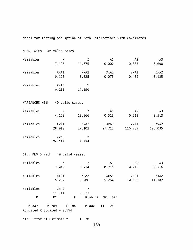
chinssitupsweightwaistProxy Variables:P_pulseP_chinsP_situps
Analysis for P_pulseDependent: pulseIndependent: chinssitupsweightwaist
MeansVariables chins situps weight waist pulse
9.450 145.550 178.600 35.400 56.100
Standard DeviationsVariables chins situps weight waist pulse
5.286 62.567 24.691 3.202 7.210
No. of valid cases = 20
CORRELATION MATRIX VARIABLE chins situps weight waist pulse chins 1.000 0.696 -0.390 -0.552 0.151 situps 0.696 1.000 -0.493 -0.646 0.225 weight -0.390 -0.493 1.000 0.870 -0.366 waist -0.552 -0.646 0.870 1.000 -0.353 pulse 0.151 0.225 -0.366 -0.353 1.000
Dependent variable: pulse
Variable Beta B Std.Err. t Prob.>t VIF TOL chins -0.062 -0.084 0.468 -0.179 0.860 2.055 0.487 situps 0.059 0.007 0.043 0.158 0.876 2.409 0.415 weight -0.235 -0.069 0.146 -0.471 0.644 4.360 0.229 waist -0.144 -0.325 1.301 -0.249 0.806 5.832 0.171 Intercept 0.000 79.673 32.257 2.470 0.026
SOURCE DF SS MS F Prob.>FRegression 4 139.176 34.794 0.615 0.6584Residual 15 848.624 56.575Total 19 987.800
R2 = 0.1409, F = 0.62, D.F. = 4 15, Prob>F = 0.6584Adjusted R2 = -0.0882Standard Error of Estimate = 7.52
159

Analysis for P_chinsDependent: chinsIndependent: pulsesitupsweightwaist
MeansVariables pulse situps weight waist chins
56.100 145.550 178.600 35.400 9.450
Standard DeviationsVariables pulse situps weight waist chins
7.210 62.567 24.691 3.202 5.286
No. of valid cases = 20
CORRELATION MATRIX VARIABLE pulse situps weight waist chins pulse 1.000 0.225 -0.366 -0.353 0.151 situps 0.225 1.000 -0.493 -0.646 0.696 weight -0.366 -0.493 1.000 0.870 -0.390 waist -0.353 -0.646 0.870 1.000 -0.552 chins 0.151 0.696 -0.390 -0.552 1.000
Dependent variable: chins
Variable Beta B Std.Err. t Prob.>t VIF TOL pulse -0.035 -0.026 0.142 -0.179 0.860 1.162 0.861 situps 0.557 0.047 0.020 2.323 0.035 1.775 0.564 weight 0.208 0.045 0.080 0.556 0.586 4.335 0.231 waist -0.386 -0.638 0.700 -0.911 0.377 5.549 0.180 Intercept 0.000 18.641 20.533 0.908 0.378
SOURCE DF SS MS F Prob.>FRegression 4 273.089 68.272 3.971 0.0216Residual 15 257.861 17.191Total 19 530.950
R2 = 0.5143, F = 3.97, D.F. = 4 15, Prob>F = 0.0216Adjusted R2 = 0.3848Standard Error of Estimate = 4.15
Analysis for P_situpsDependent: situpsIndependent: pulsechinsweight
160

waist
MeansVariables pulse chins weight waist situps
56.100 9.450 178.600 35.400 145.550
Standard DeviationsVariables pulse chins weight waist situps
7.210 5.286 24.691 3.202 62.567
No. of valid cases = 20
CORRELATION MATRIX VARIABLE pulse chins weight waist situps pulse 1.000 0.151 -0.366 -0.353 0.225 chins 0.151 1.000 -0.390 -0.552 0.696 weight -0.366 -0.390 1.000 0.870 -0.493 waist -0.353 -0.552 0.870 1.000 -0.646 situps 0.225 0.696 -0.493 -0.646 1.000
Dependent variable: situps
Variable Beta B Std.Err. t Prob.>t VIF TOL pulse 0.028 0.246 1.555 0.158 0.876 1.162 0.861 chins 0.475 5.624 2.421 2.323 0.035 1.514 0.660 weight 0.112 0.284 0.883 0.322 0.752 4.394 0.228 waist -0.471 -9.200 7.492 -1.228 0.238 5.322 0.188 Intercept 0.000 353.506 211.726 1.670 0.116
SOURCE DF SS MS F Prob.>FRegression 4 43556.048 10889.012 5.299 0.0073Residual 15 30820.902 2054.727Total 19 74376.950
R2 = 0.5856, F = 5.30, D.F. = 4 15, Prob>F = 0.0073Adjusted R2 = 0.4751Standard Error of Estimate = 45.33
Second Stage (Final) Results
MeansVariables P_pulse P_chins P_situps jumps
56.100 9.450 145.550 70.300
Standard DeviationsVariables P_pulse P_chins P_situps jumps
2.706 3.791 47.879 51.277
No. of valid cases = 20
CORRELATION MATRIX
161

VARIABLE P_pulse P_chins P_situps jumps P_pulse 1.000 0.671 0.699 0.239 P_chins 0.671 1.000 0.847 0.555 P_situps 0.699 0.847 1.000 0.394 jumps 0.239 0.555 0.394 1.000
Dependent variable: jumps
Variable Beta B Std.Err. t Prob.>t VIF TOL P_pulse -0.200 -3.794 5.460 -0.695 0.497 2.041 0.490 P_chins 0.841 11.381 5.249 2.168 0.046 3.701 0.270 P_situps -0.179 -0.192 0.431 -0.445 0.662 3.979 0.251 Intercept 0.000 203.516 277.262 0.734 0.474
SOURCE DF SS MS F Prob.>FRegression 3 17431.811 5810.604 2.858 0.0698Residual 16 32526.389 2032.899Total 19 49958.200
R2 = 0.3489, F = 2.86, D.F. = 3 16, Prob>F = 0.0698Adjusted R2 = 0.2269Standard Error of Estimate = 45.09
162

Non-Linear Regression
As an example, I have created a "parabola" function data set labeled parabola.TAB. To generate this file I used the equation y = a + b * x + c * x * x. I let a = 0, b = 5 and c = 2 for the parameters and used a sequence of x values for the independent variables in the data file that was generated. To test the non-linear fit program, I initiated the procedure and entered the values shown below:
Figure 9.11 Non-Linear Regression Specifications Form
You can see that y is the dependent variable and x is the independent variable. Values of 1 have been entered for the initial estimates of a, b and c. The equation model was selected by clicking the parabola model from the drop-down models box. I could have entered the same equation by clicking on the equation box and typing the equation into that box or clicking parameters, math functions and variables from the drop-down boxes on the right side of the form. Notice that I selected to plot the x versus y values and also the predicted versus observed y values. I also chose to save the predicted scores and residuals (y - predicted y.) The results are as follows:
163

Figure 9.12 Scores Predicted by Non-Linear Regression Versus Observed Scores
The printed output shown below gives the model selected followed by the individual data points observed, their predicted scores, the residual, the standard error of estimate of the predicted score and the 95% confidence interval of the predicted score. These are followed by the obtained correlation coefficient and its square, root mean square of the y scores, the parameter estimates with their confidence limits and t probability for testing the significance of difference from zero.
y = a + b * x1 + c * x1 * x1
x y yc y-yc SEest YcLo YcHi
0.39800 2.31000 2.30863 0.00137 0.00161 2.30582 2.31143
-1.19700 -3.13000 -3.12160 -0.00840 0.00251 -3.12597 -3.11723
-0.48600 -1.95000 -1.95878 0.00878 0.00195 -1.96218 -1.95538
-1.90800 -2.26000 -2.26113 0.00113 0.00522 -2.27020 -2.25205
-0.84100 -2.79000 -2.79228 0.00228 0.00206 -2.79586 -2.78871
-0.30100 -1.32000 -1.32450 0.00450 0.00192 -1.32784 -1.32115 164

0.69600 4.44000 4.45208 -0.01208 0.00168 4.44917 4.45500
1.11600 8.08000 8.07654 0.00346 0.00264 8.07195 8.08112
0.47900 2.86000 2.85607 0.00393 0.00159 2.85330 2.85884
1.09900 7.92000 7.91612 0.00388 0.00258 7.91164 7.92061
-0.94400 -2.94000 -2.93971 -0.00029 0.00214 -2.94343 -2.93600
-0.21800 -0.99000 -0.99541 0.00541 0.00190 -0.99872 -0.99211
0.81000 5.37000 5.36605 0.00395 0.00183 5.36288 5.36923
-0.06200 -0.31000 -0.30228 -0.00772 0.00185 -0.30549 -0.29907
0.67200 4.26000 4.26629 -0.00629 0.00165 4.26342 4.26917
-0.01900 -0.10000 -0.09410 -0.00590 0.00183 -0.09728 -0.09093
0.00100 0.01000 0.00525 0.00475 0.00182 0.00209 0.00841
0.01600 0.08000 0.08081 -0.00081 0.00181 0.07766 0.08396
1.19900 8.88000 8.87635 0.00365 0.00295 8.87122 8.88148
0.98000 6.82000 6.82561 -0.00561 0.00221 6.82177 6.82945
Corr. Coeff. = 1.00000 R2 = 1.00000
RMS Error = 5.99831, d.f. = 17 SSq = 611.65460
Parameter Estimates ...
p1= 0.00024 +/- 0.00182 p= 0.89626
p2= 5.00349 +/- 0.00171 p= 0.00000
p3= 2.00120 +/- 0.00170 p= 0.00000
Covariance Matrix Terms and Error-Correlations...
B(1,1)= 0.00000; r= 1.00000
B(1,2)=B(2,1)= -0.00000; r= -0.28318
B(1,3)=B(3,1)= -0.00000; r= -0.67166
B(2,2)= 0.00000; r= 1.00000
B(2,3)=B(3,2)= 0.00000; r= 0.32845
B(3,3)= 0.00000; r= 1.00000
165

X versus Y Plot
X = Y, Y = Y' from file: C:\Documents and Settings\Owner\My Documents\Projects\Clanguage\OpenStat\Parabola.TAB
Variable Mean Variance Std.Dev.
Y 1.76 16.29 4.04
Y' 1.76 16.29 4.04
Correlation = 1.0000, Slope = 1.00, Intercept = 0.00
Standard Error of Estimate = 0.01
Number of good cases = 20
Figure 9.13 Correlation Plot Between Scores Predicted by Non-Linear Regression and Observed Scores
You can see that the fit is quite good between the observed and predicted scores. Once you have obtained the results you will notice that the parameters, their standard errors and the t probabilities are also entered in the dialog form. Had you elected to proceed in a step-fashion, these results would be updated at each step so you can observe the convergence to the best fit (the root mean square shown in the lower left corner.)
166

Figure 111. Completed Non-Linear Regession Parameter Estimates of Regression Coefficients
IX. Multivariate
Figure 9.14 Completed Non-Linear Regression Parameter Estimates of Regression Coefficients
167

Discriminant Function / MANOVA
An Example
We will use the file labeled ManoDiscrim.txt for our example. A file of the same name (or a .tab file) should be in your directory. Load the file and then click on the Statistics / Multivariate / Discriminant Function option. You should see the form below completed for a discriminant function analysis:
Figure 9.15 Specifications for a Discriminant Function Analysis
You will notice we have asked for all options and have specified that classification use the a priori (sample) sizes for classification. When you click the Compute button, the following results are obtained:
MULTIVARIATE ANOVA / DISCRIMINANT FUNCTIONReference: Multiple Regression in Behavioral ResearchElazar J. Pedhazur, 1997, Chapters 20-21Harcourt Brace College Publishers
Total Cases := 15, Number of Groups := 3
SUM OF CROSS-PRODUCTS forGroup 1, N = 5 with 5 valid cases.
Variables Y1 Y2
168

Y1 111.000 194.000 Y2 194.000 343.000
WITHIN GROUP SUM OF DEVIATION CROSS-PROD with 5 valid cases.
Variables Y1 Y2 Y1 5.200 5.400 Y2 5.400 6.800
MEANS FOR GROUP 1, N := 5 with 5 valid cases.
Variables Y1 Y2 4.600 8.200
VARIANCES FOR GROUP 1 with 5 valid cases.
Variables Y1 Y2 1.300 1.700
STANDARD DEVIATIONS FOR GROUP 1 with 5 valid cases.
Variables Y1 Y2 1.140 1.304
SUM OF CROSS-PRODUCTS forGroup 2, N = 5 with 5 valid cases.
Variables Y1 Y2 Y1 129.000 169.000 Y2 169.000 223.000
WITHIN GROUP SUM OF DEVIATION CROSS-PROD with 5 valid cases.
Variables Y1 Y2 Y1 4.000 4.000 Y2 4.000 5.200
MEANS FOR GROUP 2, N := 5 with 5 valid cases.
169

Variables Y1 Y2 5.000 6.600
VARIANCES FOR GROUP 2 with 5 valid cases.
Variables Y1 Y2 1.000 1.300
STANDARD DEVIATIONS FOR GROUP 2 with 5 valid cases.
Variables Y1 Y2 1.000 1.140
SUM OF CROSS-PRODUCTS forGroup 3, N = 5 with 5 valid cases.
Variables Y1 Y2 Y1 195.000 196.000 Y2 196.000 199.000
WITHIN GROUP SUM OF DEVIATION CROSS-PROD with 5 valid cases.
Variables Y1 Y2 Y1 2.800 3.800 Y2 3.800 6.800
MEANS FOR GROUP 3, N := 5 with 5 valid cases.
Variables Y1 Y2 6.200 6.200
VARIANCES FOR GROUP 3 with 5 valid cases.
Variables Y1 Y2 0.700 1.700
STANDARD DEVIATIONS FOR GROUP 3 with 5 valid cases.
Variables Y1 Y2 0.837 1.304
170
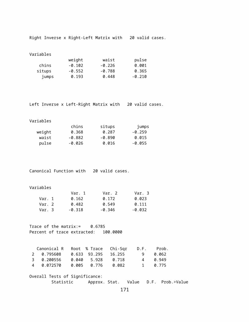
TOTAL SUM OF CROSS-PRODUCTS with 15 valid cases.
Variables Y1 Y2 Y1 435.000 559.000 Y2 559.000 765.000
TOTAL SUM OF DEVIATION CROSS-PRODUCTS with 15 valid cases.
Variables Y1 Y2 Y1 18.933 6.000 Y2 6.000 30.000
MEANS with 15 valid cases.
Variables Y1 Y2 5.267 7.000
VARIANCES with 15 valid cases.
Variables Y1 Y2 1.352 2.143
STANDARD DEVIATIONS with 15 valid cases.
Variables Y1 Y2 1.163 1.464
BETWEEN GROUPS SUM OF DEV. CPs with 15 valid cases.
Variables Y1 Y2 Y1 6.933 -7.200 Y2 -7.200 11.200
UNIVARIATE ANOVA FOR VARIABLE Y1 SOURCE DF SS MS F PROB > FBETWEEN 2 6.933 3.467 3.467 0.065ERROR 12 12.000 1.000TOTAL 14 18.933
UNIVARIATE ANOVA FOR VARIABLE Y2 SOURCE DF SS MS F PROB > FBETWEEN 2 11.200 5.600 3.574 0.061ERROR 12 18.800 1.567TOTAL 14 30.000
Inv. of Pooled Within Dev. CPs Matrix with 15 valid cases.
171

Variables Y1 Y2 Y1 0.366 -0.257 Y2 -0.257 0.234
Number of roots extracted := 2Percent of trace extracted := 100.0000Roots of the W inverse time B Matrix
No. Root Proportion Canonical R Chi-Squared D.F. Prob. 1 8.7985 0.9935 0.9476 25.7156 4 0.000 2 0.0571 0.0065 0.2325 0.6111 1 0.434
Eigenvectors of the W inverse x B Matrix with 15 valid cases.
Variables 1 2 Y1 -2.316 0.188 Y2 1.853 0.148
Pooled Within-Groups Covariance Matrix with 15 valid cases.
Variables Y1 Y2 Y1 1.000 1.100 Y2 1.100 1.567
Total Covariance Matrix with 15 valid cases.
Variables Y1 Y2 Y1 1.352 0.429 Y2 0.429 2.143
Raw Function Coeff.s from Pooled Cov. with 15 valid cases.
Variables 1 2 Y1 -2.030 0.520 Y2 1.624 0.409
Raw Discriminant Function Constants with 15 valid cases.
Variables 1 2 -0.674 -5.601
172

Fisher Discriminant FunctionsGroup 1 Constant := -24.402Variable Coefficient 1 -5.084 2 8.804
Group 2 Constant := -14.196Variable Coefficient 1 1.607 2 3.084Group 3 Constant := -19.759Variable Coefficient 1 8.112 2 -1.738
CLASSIFICATION OF CASESSUBJECT ACTUAL HIGH PROBABILITY SEC.D HIGH DISCRIMID NO. GROUP IN GROUP P(G/D) GROUP P(G/D) SCORE 1 1 1 0.9999 2 0.0001 4.6019 -1.1792 2 1 1 0.9554 2 0.0446 2.5716 -0.6590 3 1 1 0.8903 2 0.1097 2.1652 0.2699 4 1 1 0.9996 2 0.0004 3.7890 0.6786 5 1 1 0.9989 2 0.0011 3.3826 1.6075 6 2 2 0.9746 3 0.0252 -0.6760 -1.4763 7 2 2 0.9341 1 0.0657 0.9478 -1.0676 8 2 2 0.9730 1 0.0259 0.5414 -0.1387 9 2 2 0.5724 3 0.4276 -1.4888 0.3815 10 2 2 0.9842 1 0.0099 0.1350 0.7902 11 3 3 0.9452 2 0.0548 -2.7062 -0.9560 12 3 3 0.9999 2 0.0001 -4.7365 -0.4358 13 3 3 0.9893 2 0.0107 -3.1126 -0.0271 14 3 3 0.9980 2 0.0020 -3.5191 0.9018 15 3 3 0.8007 2 0.1993 -1.8953 1.3104
CLASSIFICATION TABLE
173

PREDICTED GROUPVariables 1 2 3 TOTAL 1 5 0 0 5 2 0 5 0 5 3 0 0 5 5 TOTAL 5 5 5 15
Standardized Coeff. from Pooled Cov. with 15 valid cases.
Variables 1 2 Y1 -2.030 0.520 Y2 2.032 0.511
Centroids with 15 valid cases.
Variables 1 2 1 3.302 0.144 2 -0.108 -0.302 3 -3.194 0.159
Raw Coefficients from Total Cov. with 15 valid cases.
Variables 1 2 Y1 -0.701 0.547 Y2 0.560 0.429
Raw Discriminant Function Constants with 15 valid cases.
Variables 1 2 -0.674 -5.601
Standardized Coeff.s from Total Cov. with 15 valid cases.
Variables 1 2 Y1 -0.815 0.636 Y2 0.820 0.628
Total Correlation Matrix with 15 valid cases.
174

Variables Y1 Y2 Y1 1.000 0.252 Y2 0.252 1.000
Corr.s Between Variables and Functions with 15 valid cases.
Variables 1 2 Y1 -0.608 0.794 Y2 0.615 0.788
Wilk's Lambda = 0.0965.F = 12.2013 with D.F. 4 and 22 . Prob > F = 0.0000
Bartlett Chi-Squared = 26.8845 with 4 D.F. and prob. = 0.0000
Figure 9.16 Plot of Cases in the Discriminant Space
Pillai Trace = 0.9520
You will notice that we have obtained cross-products and deviation cross-products for each group as well as the combined between and within groups as well as descriptive statistics (means, variances, standard deviations.) Two roots were obtained, the first significant at the 0.05 level using a chi-square test. The one-way analyses of variances completed for each continuous variable were not significant at the 0.05 level which demonstrates that a multivariate analysis may identify group differences not caught by individual variable analysis. The discriminant functions can be used to plot the group subjects in the (orthogonal) space of the functions. If you examine the plot
175

you can see that the individuals in the three groups analyzed are easily separated using just the first discriminant function (the horizontal axis.) Raw and standardized coefficients for the discriminant functions are presented as well as Fisher’s discriminant functions for each group. The latter are used to classify the subjects and the classifications are shown along with a table which summarizes the classifications. Note that in this example, all cases are correctly classified. Certainly, a cross-validation of the functions for classification would likely encounter some errors of classification. Since we asked that the discriminant scores be placed in the data grid, the last figure shows the data grid with the Fisher discriminant scores saved as two new variables.
Cluster Analyses
Hierarchical Cluster Analysis
To demonstrate the Hierarchical Clustering program, the data to be analyzed is the one labeled cansas.TAB. You will see the form below with specifications for the grouping:
Figure 9.17 Hierarchical Cluster Analysis Form
Results for the hierarchical analysis that you would obtain after clicking the Compute button are presented below:
Hierarchical Cluster Analysis
Number of object to cluster = 20 on 6 variables.
Variable Means
176
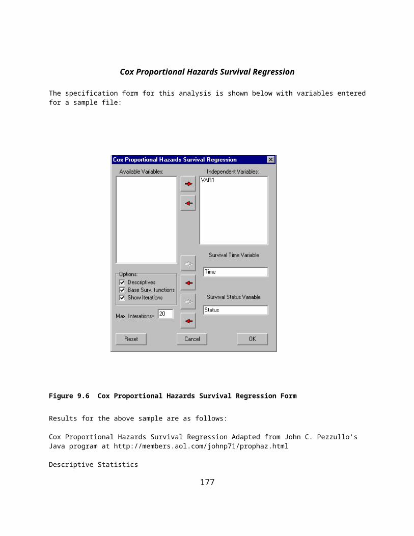
Variables weight waist pulse chins situps jumps 178.600 35.400 56.100 9.450 145.550 70.300
Variable Variances
Variables weight waist pulse chins situps jumps 609.621 10.253 51.989 27.945 3914.576 2629.379
Variable Standard Deviations
Variables weight waist pulse chins situps jumps 24.691 3.202 7.210 5.286 62.567 51.277
19 groups after combining group 1 (n = 1 ) and group 5 (n = 1) error = 0.386
18 groups after combining group 17 (n = 1 ) and group 18 (n = 1) error = 0.387
17 groups after combining group 11 (n = 1 ) and group 17 (n = 2) error = 0.556
16 groups after combining group 1 (n = 2 ) and group 16 (n = 1) error = 0.663
15 groups after combining group 3 (n = 1 ) and group 7 (n = 1) error = 0.805
14 groups after combining group 4 (n = 1 ) and group 10 (n = 1) error = 1.050
13 groups after combining group 2 (n = 1 ) and group 6 (n = 1) error = 1.345
12 groups after combining group 1 (n = 3 ) and group 14 (n = 1) error = 1.402
11 groups after combining group 0 (n = 1 ) and group 1 (n = 4) error = 1.489
10 groups after combining group 11 (n = 3 ) and group 12 (n = 1) error = 2.128Group 1 (n= 5) Object = CASE 1 Object = CASE 2 Object = CASE 6 Object = CASE 15 Object = CASE 17Group 3 (n= 2) Object = CASE 3 Object = CASE 7Group 4 (n= 2) Object = CASE 4 Object = CASE 8Group 5 (n= 2) Object = CASE 5
177

Object = CASE 11Group 9 (n= 1) Object = CASE 9Group 10 (n= 1) Object = CASE 10Group 12 (n= 4) Object = CASE 12 Object = CASE 13 Object = CASE 18 Object = CASE 19Group 14 (n= 1) Object = CASE 14Group 16 (n= 1) Object = CASE 16Group 20 (n= 1) Object = CASE 20
(…. for 9 groups, 8 groups, etc. down to 2 groups)
4 groups after combining group 4 (n = 6 ) and group 9 (n = 1) error = 11.027Group 1 (n= 8) Object = CASE 1 Object = CASE 2 Object = CASE 3 Object = CASE 6 Object = CASE 7 Object = CASE 15 Object = CASE 16 Object = CASE 17Group 4 (n= 4) Object = CASE 4 Object = CASE 8 Object = CASE 9 Object = CASE 20Group 5 (n= 7) Object = CASE 5 Object = CASE 10 Object = CASE 11 Object = CASE 12 Object = CASE 13 Object = CASE 18 Object = CASE 19Group 14 (n= 1) Object = CASE 14
3 groups after combining group 0 (n = 8 ) and group 13 (n = 1) error = 13.897Group 1 (n= 9) Object = CASE 1 Object = CASE 2 Object = CASE 3 Object = CASE 6 Object = CASE 7 Object = CASE 14 Object = CASE 15
178

Object = CASE 16 Object = CASE 17Group 4 (n= 4) Object = CASE 4 Object = CASE 8 Object = CASE 9 Object = CASE 20Group 5 (n= 7) Object = CASE 5 Object = CASE 10 Object = CASE 11 Object = CASE 12 Object = CASE 13 Object = CASE 18 Object = CASE 19
2 groups after combining group 3 (n = 4 ) and group 4 (n = 7) error = 17.198Group 1 (n= 9) Object = CASE 1 Object = CASE 2 Object = CASE 3 Object = CASE 6 Object = CASE 7 Object = CASE 14 Object = CASE 15 Object = CASE 16 Object = CASE 17Group 4 (n= 11) Object = CASE 4 Object = CASE 5 Object = CASE 8 Object = CASE 9 Object = CASE 10 Object = CASE 11 Object = CASE 12 Object = CASE 13 Object = CASE 18 Object = CASE 19 Object = CASE 20
179

SCATTERPLOT - Plot of Error vs No. of Groups
Size of Error | |- 18.06 | |- 17.20 | |- 16.34 . | |- 15.48 | |- 14.62 | |- 13.76 | |- 12.90 . | |- 12.04 | |- 11.18 | |- 10.32------------------------------------------------------------|- 9.46 . | |- 8.60 . . | |- 7.74 | |- 6.88 | |- 6.02 | |- 5.16 . . | |- 4.30 . | |- 3.44 * . . . |- 2.58 | . . . . . |- 1.72_______________________________________________________________ | | | | | | | | | | No. of Groups 2.00 4.00 6.00 8.00 10.00 12.00 14.00 16.00 18.00 20.00
Figure 9.18 Plot of Grouping Errors in the Discriminant Analysis
If you compare the results above with a discriminant analysis analysis on the same data, you will see that the clustering procedure does not necessarily replicate the original groups. Clearly, “nearest neighbor” grouping in euclidean space does not necessarily result in the same a priori groups from the discriminant analysis.
By examining the increase in error (variance of subjects within the groups) as a function of the number of groups, one can often make some decision about the number of groups they wish to interpret. There is a large increase in error when going from 8 groups down to 7 in this analysis which suggests there are possibly 7 or 8 groups which might be examined. If we had more information on the objects of those groups, we might see a pattern or commonality shared by objects of those groups.
K-Means Clustering AnalysisWith this procedure, one first specifies the number of groups to be formed among the objects. The
procedure uses a procedure to load each of the k groups with one object in a somewhat random manner. The procedure then iteratively adds or subtracts objects from each group based on an error measure of the distance between the objects in the group. The procedure ends when subsequent iterations do not produce a lower value or the number of iterations has been exceeded.
In this example, we loaded the cansas.TAB file to group the 20 subjects into four groups. The results may be compared with the other cluster methods of this chapter.
180

Figure 9.19 The K Means Clustering Form
Results are:
K-Means Clustering. Adapted from AS 136 APPL. STATIST. (1979) VOL.28, NO.1
File = C:\Documents and Settings\Owner\My Documents\Projects\Clanguage\OpenStat\cansas.TABNo. Cases = 20, No. Variables = 6, No. Clusters = 4
NUMBER OF SUBJECTS IN EACH CLUSTERCluster = 1 with 1 cases.Cluster = 2 with 7 cases.Cluster = 3 with 9 cases.Cluster = 4 with 3 cases.
PLACEMENT OF SUBJECTS IN CLUSTERSCLUSTER SUBJECT 1 14 2 2 2 6 2 8 2 1 2 15 2 17 2 20 3 11 3 12 3 13 3 4 3 5 3 9 3 18 3 19 3 10 4 7 4 16 4 3
AVERAGE VARIABLE VALUES BY CLUSTER VARIABLES
181

CLUSTER 1 2 3 4 5 6 1 0.11 1.03 -0.12 -0.30 -0.02 -0.01 2 -0.00 0.02 -0.02 -0.19 -0.01 -0.01 3 -0.02 -0.20 0.01 0.17 0.01 0.01 4 0.04 0.22 0.05 0.04 -0.00 0.01
WITHIN CLUSTER SUMS OF SQUARESCluster 1 = 0.000Cluster 2 = 0.274Cluster 3 = 0.406Cluster 4 = 0.028
Average Linkage Hierarchical Cluster Analysis
This cluster procedure clusters objects based on their similarity (or dissimilarity) as recorded in a data matrix. The correlation among objects is often used as a measure of similarity. In this example, we first loaded the file labeled "cansas.TAB". We then "rotated" the data using the rotate function in the Edit menu so that columns represent subjects and rows represent variables. We then used the Correlation procedure (with the option to save the correlation matrix) to obtain the correlation among the 20 subjects as a measure of similarity. We then closed the file. Next, we opened the matrix file we had just saved using the File / Open a Matrix File option. We then clicked on the Analyses / Multivariate / Cluster / Average Linkage option. Shown below is the dialogue box for the analysis:
Figure 9.20 Average Linkage Dialog Form
Output of the analysis includes a listing of which objects (groups) are combined at each step followed by a dendogram of the combinations. You can compare this method of clustering subjects with that obtained in the previous analysis.
Average Linkage Cluster Analysis. Adopted from ClusBas by John S. Uebersax
Group 18 is joined by group 19. N is 2 ITER = 1 SIM = 0.999Group 1 is joined by group 5. N is 2 ITER = 2 SIM = 0.998Group 6 is joined by group 7. N is 2 ITER = 3 SIM = 0.995Group 15 is joined by group 17. N is 2 ITER = 4 SIM = 0.995Group 12 is joined by group 13. N is 2 ITER = 5 SIM = 0.994Group 8 is joined by group 11. N is 2 ITER = 6 SIM = 0.993
182

Group 4 is joined by group 8. N is 3 ITER = 7 SIM = 0.992Group 2 is joined by group 6. N is 3 ITER = 8 SIM = 0.988Group 12 is joined by group 16. N is 3 ITER = 9 SIM = 0.981Group 14 is joined by group 15. N is 3 ITER = 10 SIM = 0.980Group 2 is joined by group 4. N is 6 ITER = 11 SIM = 0.978Group 12 is joined by group 18. N is 5 ITER = 12 SIM = 0.972Group 2 is joined by group 20. N is 7 ITER = 13 SIM = 0.964Group 1 is joined by group 2. N is 9 ITER = 14 SIM = 0.962Group 9 is joined by group 12. N is 6 ITER = 15 SIM = 0.933Group 1 is joined by group 3. N is 10 ITER = 16 SIM = 0.911Group 1 is joined by group 14. N is 13 ITER = 17 SIM = 0.900Group 1 is joined by group 9. N is 19 ITER = 18 SIM = 0.783Group 1 is joined by group 10. N is 20 ITER = 19 SIM = 0.558
No. of objects = 20Matrix defined similarities among objects.
UNIT 1 5 2 6 7 4 8 11 20 3 14 15 17 9 12 13 16 18 19 10STEP * * * * * * * * * * * * * * * * * * * * 1 * * * * * * * * * * * * * * * * * ****** * * * * * * * * * * * * * * * * * * * * 2 ****** * * * * * * * * * * * * * * * * * * * * * * * * * * * * * * * * * * * 3 * * ****** * * * * * * * * * * * * * * * * * * * * * * * * * * * * * * * 4 * * * * * * * * * ****** * * * * * * * * * * * * * * * * * * * * * * 5 * * * * * * * * * * * ****** * * * * * * * * * * * * * * * * * * 6 * * * * ****** * * * * * * * * * * * * * * * * * * * * * * * 7 * * * ******** * * * * * * * * * * * * * * * * * * * * * * 8 * ******** * * * * * * * * * * * * * * * * * * * * * * 9 * * * * * * * * ********* * * * * * * * * * * * * * 10 * * * * * ******** * * * * * * * * * * * * * * 11 * **************** * * * * * * *
183

* * * * * * * * * 12 * * * * * * ************ * * * * * * * * * 13 * ********************* * * * * * * * * * * * * 14 ***************************** * * * * * * * * * * * 15 * * * ***************** * * * * * * 16 ****************************** * * * * * * * 17 ************************ * * * * * 18 ********************************* * * * 19 ***************************************
184
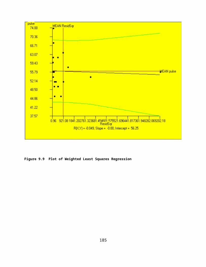
Path Analysis
To illustrate path analysis, we will utilize an example from page 788 of the book by Elazar J. Pedhazur (Multiple Regression in Behavioral Science, 1997.) Four variables in the study are labeled SES (Socio-Economic Status), IQ (Intelligence Quotient), AM (Achievement Motivation) and GPA (Grade Point Average.) Our theoretical speculations lead us to believe that AM is “caused” by SES and IQ and that GPA is “caused” by AM as well as SES and IQ. We will enter the correlations among these variables into the data grid of OpenStat then analyze the matrix with the path analysis procedure. Show below are the results.
Example of a Path Analysis
In this example we will use the file CANSAS.TXT. The user begins by selecting the Path Analysis option of the Statistics / Multivariate menu. In the figure below we have selected all variables to analyze and have entered our first path indicating that waist size is “caused” by weight:
Figure 9.21 Path Analysis Dialog Form
We will also hypothesize that pulse rate is “caused” by weight, chin-ups are “caused” by weight, waist and pulse, that the number of sit-ups is “caused” by weight, waist and pulse and that jumps are “caused” by weight, waist and pulse. Each time we enter a new causal relationship we click the scroll bar to move to a new model number prior to entering the “caused” and “causing” variables. Once we have entered each model, we then click on the Compute button. Note we have elected to print descriptive statistics, each models correlation matrix, and the reproduced correlation matrix which will be our measure of how well the models “fit” the data. The results are shown below:
185
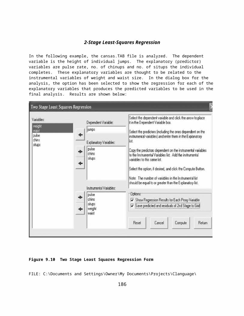
PATH ANALYSIS RESULTS
CAUSED VARIABLE: waist Causing Variables: weight CAUSED VARIABLE: pulse Causing Variables: weight CAUSED VARIABLE: chins Causing Variables: weight waist pulse CAUSED VARIABLE: situps Causing Variables: weight waist pulse CAUSED VARIABLE: jumps Causing Variables: weight waist pulse
Correlation Matrix with 20 valid cases.
Variables weight waist pulse chins situps weight 1.000 0.870 -0.366 -0.390 -0.493 waist 0.870 1.000 -0.353 -0.552 -0.646 pulse -0.366 -0.353 1.000 0.151 0.225 chins -0.390 -0.552 0.151 1.000 0.696 situps -0.493 -0.646 0.225 0.696 1.000 jumps -0.226 -0.191 0.035 0.496 0.669
Variables jumps weight -0.226 waist -0.191 pulse 0.035 chins 0.496 situps 0.669 jumps 1.000
MEANS with 20 valid cases.
Variables weight waist pulse chins situps 178.600 35.400 56.100 9.450 145.550
186
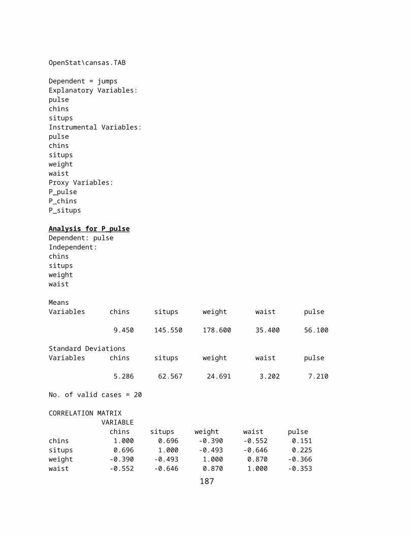
Variables jumps 70.300
VARIANCES with 20 valid cases.
Variables weight waist pulse chins situps 609.621 10.253 51.989 27.945 3914.576
Variables jumps 2629.379
STANDARD DEVIATIONS with 20 valid cases.
Variables weight waist pulse chins situps 24.691 3.202 7.210 5.286 62.567
Variables jumps 51.277
Dependent Variable = waist
Correlation Matrix with 20 valid cases.
Variables weight waist weight 1.000 0.870 waist 0.870 1.000
MEANS with 20 valid cases.
Variables weight waist 178.600 35.400
VARIANCES with 20 valid cases.
Variables weight waist 609.621 10.253
STANDARD DEVIATIONS with 20 valid cases.
Variables weight waist 24.691 3.202
187

Dependent Variable = waist
R R2 F Prob.>F DF1 DF2 0.870 0.757 56.173 0.000 1 18Adjusted R Squared = 0.744
Std. Error of Estimate = 1.621
Variable Beta B Std.Error t Prob.>t weight 0.870 0.113 0.015 7.495 0.000
Constant = 15.244
Dependent Variable = pulse
Correlation Matrix with 20 valid cases.
Variables weight pulse weight 1.000 -0.366 pulse -0.366 1.000
MEANS with 20 valid cases.
Variables weight pulse 178.600 56.100
VARIANCES with 20 valid cases.
Variables weight pulse 609.621 51.989
STANDARD DEVIATIONS with 20 valid cases.
Variables weight pulse 24.691 7.210
Dependent Variable = pulse
R R2 F Prob.>F DF1 DF2 0.366 0.134 2.780 0.113 1 18Adjusted R Squared = 0.086
Std. Error of Estimate = 6.895
Variable Beta B Std.Error t Prob.>t weight -0.366 -0.107 0.064 -1.667 0.113
Constant = 75.177
188

Dependent Variable = chins
Correlation Matrix with 20 valid cases.
Variables weight waist pulse chins weight 1.000 0.870 -0.366 -0.390 waist 0.870 1.000 -0.353 -0.552 pulse -0.366 -0.353 1.000 0.151 chins -0.390 -0.552 0.151 1.000
MEANS with 20 valid cases.
Variables weight waist pulse chins 178.600 35.400 56.100 9.450
VARIANCES with 20 valid cases.
Variables weight waist pulse chins 609.621 10.253 51.989 27.945
STANDARD DEVIATIONS with 20 valid cases.
Variables weight waist pulse chins 24.691 3.202 7.210 5.286
189

Dependent Variable = chins
R R2 F Prob.>F DF1 DF2 0.583 0.340 2.742 0.077 3 16Adjusted R Squared = 0.216
Std. Error of Estimate = 4.681
Variable Beta B Std.Error t Prob.>t weight 0.368 0.079 0.089 0.886 0.389 waist -0.882 -1.456 0.683 -2.132 0.049 pulse -0.026 -0.019 0.160 -0.118 0.907
Constant = 47.968
Dependent Variable = situps
Correlation Matrix with 20 valid cases.
Variables weight waist pulse situps weight 1.000 0.870 -0.366 -0.493 waist 0.870 1.000 -0.353 -0.646 pulse -0.366 -0.353 1.000 0.225 situps -0.493 -0.646 0.225 1.000
MEANS with 20 valid cases.
Variables weight waist pulse situps 178.600 35.400 56.100 145.550
VARIANCES with 20 valid cases.
Variables weight waist pulse situps 609.621 10.253 51.989 3914.576
STANDARD DEVIATIONS with 20 valid cases.
Variables weight waist pulse situps 24.691 3.202 7.210 62.567
190

Dependent Variable = situps
R R2 F Prob.>F DF1 DF2 0.661 0.436 4.131 0.024 3 16Adjusted R Squared = 0.331
Std. Error of Estimate = 51.181
Variable Beta B Std.Error t Prob.>t weight 0.287 0.728 0.973 0.748 0.466 waist -0.890 -17.387 7.465 -2.329 0.033 pulse 0.016 0.139 1.755 0.079 0.938
Constant = 623.282
Dependent Variable = jumps
Correlation Matrix with 20 valid cases.
Variables weight waist pulse jumps weight 1.000 0.870 -0.366 -0.226 waist 0.870 1.000 -0.353 -0.191 pulse -0.366 -0.353 1.000 0.035 jumps -0.226 -0.191 0.035 1.000
MEANS with 20 valid cases.
Variables weight waist pulse jumps 178.600 35.400 56.100 70.300
VARIANCES with 20 valid cases.
Variables weight waist pulse jumps 609.621 10.253 51.989 2629.379
STANDARD DEVIATIONS with 20 valid cases.
Variables weight waist pulse jumps 24.691 3.202 7.210 51.277
191

Dependent Variable = jumps
R R2 F Prob.>F DF1 DF2 0.232 0.054 0.304 0.822 3 16Adjusted R Squared = -0.123
Std. Error of Estimate = 54.351
Variable Beta B Std.Error t Prob.>t weight -0.259 -0.538 1.034 -0.520 0.610 waist 0.015 0.234 7.928 0.029 0.977 pulse -0.055 -0.389 1.863 -0.209 0.837
Constant = 179.887
Matrix of Path Coefficients with 20 valid cases.
Variables weight waist pulse chins situps weight 0.000 0.870 -0.366 0.368 0.287 waist 0.870 0.000 0.000 -0.882 -0.890 pulse -0.366 0.000 0.000 -0.026 0.016 chins 0.368 -0.882 -0.026 0.000 0.000 situps 0.287 -0.890 0.016 0.000 0.000 jumps -0.259 0.015 -0.055 0.000 0.000
Variables jumps weight -0.259 waist 0.015 pulse -0.055 chins 0.000 situps 0.000 jumps 0.000
192
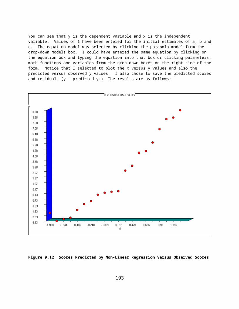
SUMMARY OF CAUSAL MODELSVar. Caused Causing Var. Path Coefficient waist weight 0.870 pulse weight -0.366 chins weight 0.368 chins waist -0.882 chins pulse -0.026 situps weight 0.287 situps waist -0.890 situps pulse 0.016 jumps weight -0.259 jumps waist 0.015 jumps pulse -0.055
Reproduced Correlation Matrix with 20 valid cases.
Variables weight waist pulse chins situps weight 1.000 0.870 -0.366 -0.390 -0.493 waist 0.870 1.000 -0.318 -0.553 -0.645 pulse -0.366 -0.318 1.000 0.120 0.194 chins -0.390 -0.553 0.120 1.000 0.382 situps -0.493 -0.645 0.194 0.382 1.000 jumps -0.226 -0.193 0.035 0.086 0.108
Variables jumps weight -0.226 waist -0.193 pulse 0.035 chins 0.086 situps 0.108 jumps 1.000
Average absolute difference between observed and reproducedcoefficients := 0.077Maximum difference found := 0.562
We note that pulse is not a particularly important predictor of chin-ups or sit-ups. The largest discrepancy of 0.562 between an original correlation and a correlation reproduced using the path coefficients indicates our model of causation may have been inadequate.
193

Factor Analysis
The sample factor analysis completed below utilizes a data set labeled CANSAS.TXT as used in the previous path analysis example . The canonical factor analysis method was used andthe varimax rotation method was used.
Shown below is the factor analysis form selected by choosing the factor analysis option under the Statistics / Multivariate menu:
Figure 9.22 Factor Analysis Dialog Form
Note the options elected in the above form. The results obtained are shown below:
194

Figure 9.23 Scree Plot of Eigenvalues
Factor AnalysisSee Rummel, R.J., Applied Factor AnalysisNorthwestern University Press, 1970
Canonical Factor AnalysisOriginal matrix trace = 18.56Roots (Eigenvalues) Extracted: 1 15.512 2 3.455 3 0.405 4 0.010 5 -0.185 6 -0.641
Unrotated Factor Loadings
FACTORS with 20 valid cases.
Variables Factor 1 Factor 2 Factor 3 Factor 4 Factor 5 weight 0.858 -0.286 0.157 -0.006 0.000 waist 0.928 -0.201 -0.066 -0.003 0.000 pulse -0.360 0.149 -0.044 -0.089 0.000 chins -0.644 -0.382 0.195 0.009 0.000 situps -0.770 -0.472 0.057 -0.009 0.000 jumps -0.409 -0.689 -0.222 0.005 0.000
195

Variables Factor 6 weight 0.000 waist 0.000 pulse 0.000 chins 0.000 situps 0.000 jumps 0.000
Percent of Trace In Each Root: 1 Root := 15.512 Trace := 18.557 Percent := 83.593 2 Root := 3.455 Trace := 18.557 Percent := 18.621 3 Root := 0.405 Trace := 18.557 Percent := 2.180 4 Root := 0.010 Trace := 18.557 Percent := 0.055 5 Root := -0.185 Trace := 18.557 Percent := -0.995 6 Root := -0.641 Trace := 18.557 Percent := -3.455
COMMUNALITY ESTIMATES 1 weight 0.844 2 waist 0.906 3 pulse 0.162 4 chins 0.598 5 situps 0.819 6 jumps 0.692
Proportion of variance in unrotated factors
1 48.364 2 16.475
Communality Estimates as percentages: 1 81.893 2 90.153 3 15.165 4 56.003 5 81.607 6 64.217
Varimax Rotated Loadings with 20 valid cases.
Variables Factor 1 Factor 2 weight -0.882 -0.201 waist -0.898 -0.310 pulse 0.385 0.059 chins 0.352 0.660 situps 0.413 0.803 jumps -0.009 0.801
196
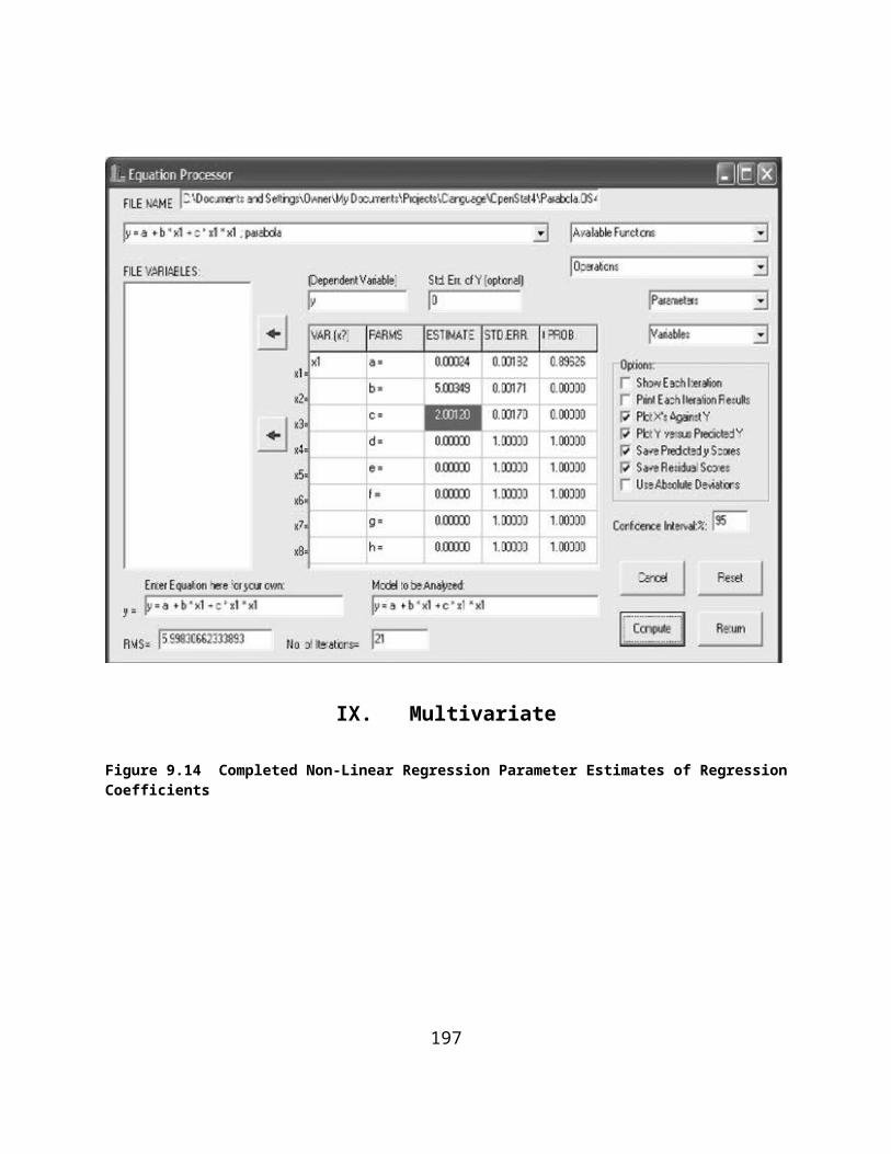
Percent of Variation in Rotated FactorsFactor 1 33.776Factor 2 31.064
Total Percent of Variance in Factors : 64.840Communalities as Percentages 1 for weight 81.893 2 for waist 90.153 3 for pulse 15.165 4 for chins 56.003 5 for situps 81.607 6 for jumps 64.217
197

SCATTERPLOT - FACTOR PLOT
Factor 2 | | |- 0.95- 1.00 | | |- 0.90- 0.95 | | |- 0.85- 0.90 | 2 1 |- 0.80- 0.85 | | |- 0.75- 0.80 | | |- 0.70- 0.75 | | 3 |- 0.65- 0.70 | | |- 0.60- 0.65 | | |- 0.55- 0.60 | | |- 0.50- 0.55 | | |- 0.45- 0.50 | | |- 0.40- 0.45 | | |- 0.35- 0.40 | | |- 0.30- 0.35 | | |- 0.25- 0.30 | | |- 0.20- 0.25 | | |- 0.15- 0.20 | | |- 0.10- 0.15 | | 4 |- 0.05- 0.10 |------------------------------------------------------------|- 0.00- 0.05 | | |- -0.05- 0.00 | | |- -0.10- -0.05 | | |- -0.15- -0.10 | | |- -0.20- -0.15 | 5 | |- -0.25- -0.20 | | |- -0.30- -0.25 | 6 | |- -0.35- -0.30 | | |- -0.40- -0.35 | | |- -0.45- -0.40 | | |- -0.50- -0.45 | | |- -0.55- -0.50 | | |- -0.60- -0.55 | | |- -0.65- -0.60 | | |- -0.70- -0.65 | | |- -0.75- -0.70 | | |- -0.80- -0.75 | | |- -0.85- -0.80 | | |- -0.90- -0.85 | | |- -0.95- -0.90 | | |- -1.00- -0.95--------------------------------------------------------------- | | | | | | | | | | | | | | | | Factor 1-1.0-0.9-0.7-0.6-0.5-0.3-0.2-0.1 0.1 0.2 0.3 0.5 0.6 0.7 0.9 1.0
Labels: 1 = situps 2 = jumps 3 = chins 4 = pulse 5 = weight
198

6 = waist
SUBJECT FACTOR SCORE RESULTS:
Regression Coefficients with 20 valid cases.
Variables Factor 1 Factor 2 weight -0.418 0.150 waist -0.608 0.080 pulse 0.042 -0.020 chins -0.024 0.203 situps -0.069 0.526 jumps -0.163 0.399
Standard Error of Factor Scores:Factor 1 0.946Factor 2 0.905
We note that two factors were extracted with eigenvalues greater than 1.0 and when rotated indicate that the three body measurements appear to load on one factor and that the performance measures load on the second factor. The data grid also now contains the “least-squares” factor scores for each subject. Hummm! I wonder what a hierarchical grouping of these subjects on the two factor scores would produce!
199

General Linear Model (Sums of Squares by Regression)
Two examples will be provided in this section. The first example demonstrates the use of the GLM procedure for completing a three-way analysis of variance. The second will demonstrate the use of the GLM procedure a repeated measures analysis of variance. Alternative procedures will also be presented to aid in the interpretation of the results.
Example 1
The file labeled Ancova3.tab is loaded. Next, select the Analyses / Multivariate / Sums of Squares by Regression option from the menu. Shown below is the form for specifying a three-way, analysis of covariance. The dependent variable X has been entered in the continuous dependent variable list. The independent variables Row, Column, Slice have been entered in the fixed effects dependent list box. The two covariates have been entered in the covariates box. The coding method elected for creating vectors representing the categories of the independent variables is the orthogonal coding method. To specify the interactions for the analysis model, the button “begin definition of an interaction” is clicked followed by clicking of each term to be included in the interaction. The specification of the interaction is ended by clicking the “end definition of an interaction” button. This procedure was repeated for each of the interactions desired: row by column, row by slice, column by slice and row by column by slice. You will note that these interaction definitions are summarized using abbreviations in the list of defined interactions. You may also select the output options desired before clicking the “Compute” button. It is suggested that you select the option for all multiple regression results only if you wish to fully understand how the analysis is completed since the output is voluminous. The output shown below is the result of NOT selecting any of the options.
200

Figure 9.24 The GLM Dialog Form
The results obtained are shown below. Each predictor (coded vector) is entered one-by-one with the increment in variance (squared multiple correlation). This is then followed by computing the full model (the model with all variables entered) minus each independent variable to obtain the decrement in variance associated with each specific independent variable. Again, for brevity, this part of the output is not shown. A summary table then provides the results of the incremental and decrement effect of each variable. The final table summarizes the results for the analysis of variance. You will notice that, through the use of orthogonal coding, we can verify the independence of the row, column and slice effect variables. The inter-correlation among the coding vectors for a balanced design will be zero (0.0). Attempting to do a three-way analysis of variance using the traditional “partitioning of variance” method may result in a program error when a design is unbalanced, that is, the cell sizes are not equal or proportional across the factors. The unique contributions of each factor can, however, be assessed using multiple regression as in the general linear model.
------------------------------------------------------------------------------------------SUMS OF SQUARES AND MEAN SQUARES BY REGRESSIONTYPE III SS - R2 = Full Model - Restricted Model
VARIABLE SUM OF SQUARES D.F.
Cov1 1.275 1 Cov2 0.783 1 Row1 25.982 1 Col1 71.953 1 Slice1 13.323 1 Slice2 0.334 1 C1R1 21.240 1 S1R1 11.807 1 S2R1 0.138 1 S1C1 13.133 1 S2C1 0.822 1 S1C1R1 0.081 1 S2C1R1 47.203 1ERROR 46.198 58TOTAL 269.500 71
TOTAL EFFECTS SUMMARY-----------------------------------------------------------SOURCE SS D.F. MS----------------------------------------------------------- Cov1 1.275 1 1.275 Cov2 0.783 1 0.783 Row 25.982 1 25.982 Col 71.953 1 71.953 Slice 13.874 2 6.937 Row*Col 21.240 1 21.240 Row*Slice 11.893 2 5.947 Col*Slice 14.204 2 7.102 Row*Col*Slice 47.247 2 23.624-----------------------------------------------------------
-----------------------------------------------------------SOURCE SS D.F. MS-----------------------------------------------------------
201

BETWEEN SUBJECTS 208.452 13 Covariates 2.058 2 1.029 Row 25.982 1 25.982 Col 71.953 1 71.953 Slice 13.874 2 6.937 Row*Col 21.240 1 21.240 Row*Slice 11.893 2 5.947 Col*Slice 14.204 2 7.102 Row*Col*Slice 47.247 2 23.624ERROR BETWEEN 46.198 58 0.797
-----------------------------------------------------------
-----------------------------------------------------------TOTAL 269.500 71-----------------------------------------------------------
The output above may be compared with the results obtained using the analysis of covariance procedure under the Analysis of Variance menu. The results from that analysis are shown next. You can see that the results are essentially identical although the ANCOVA procedure also includes some tests of the assumptions of homogeneity.
Test for Homogeneity of Group Regression CoefficientsChange in R2 = 0.1629. F = 31.437 Prob.> F = 0.0000 with d.f. 22 and 36Unadjusted Group Means for Group Variables Row MeansVariables Group 1 Group 2
3.500 4.667
Intercepts for Each Group Regression Equation for Variable: Row InterceptsVariables Group 1 Group 2
4.156 5.404
Adjusted Group Means for Group Variables Row MeansVariables Group 1 Group 2
3.459 4.707
Unadjusted Group Means for Group Variables Col MeansVariables Group 1 Group 2
3.000 5.167
Intercepts for Each Group Regression Equation for Variable: Col InterceptsVariables Group 1 Group 2
202

4.156 5.404
Adjusted Group Means for Group Variables Col MeansVariables Group 1 Group 2
2.979 5.187
Unadjusted Group Means for Group Variables Slice MeansVariables Group 1 Group 2 Group 3
3.500 4.500 4.250
Intercepts for Each Group Regression Equation for Variable: Slice InterceptsVariables Group 1 Group 2 Group 3
4.156 3.676 6.508
Adjusted Group Means for Group Variables Slice MeansVariables Group 1 Group 2 Group 3
3.493 4.572 4.185
Test for Each Source of Variance Obtained by Eliminatingfrom the Regression Model for ANCOVA the Vectors Associatedwith Each Fixed Effect.
---------------------------------------------------------------------- SOURCE Deg.F. SS MS F Prob>F---------------------------------------------------------------------- Cov1 1 1.27 1.27 1.600 0.2109 Cov2 1 0.78 0.78 0.983 0.3255 A 1 25.98 25.98 32.620 0.0000 B 1 71.95 71.95 90.335 0.0000 C 2 13.87 6.94 8.709 0.0005 AxB 1 21.24 21.24 26.666 0.0000 AxC 2 11.89 5.95 7.466 0.0013 BxC 2 14.20 7.10 8.916 0.0004 AxBxC 2 47.25 23.62 29.659 0.0000---------------------------------------------------------------------- ERROR 58 46.20 0.80---------------------------------------------------------------------- TOTAL 71 269.50----------------------------------------------------------------------
----------------------------------------------------------------------ANALYSIS FOR COVARIATES ONLYCovariates 2 6.99 3.49 0.918 0.4041----------------------------------------------------------------------
203

Example Two
The second example of the GLM procedure involves a repeated measures analysis of variance similar to that you might complete with the "two between and one within anova" procedure. In this example, we have used the file labeled REGSS2.TAB. The data include a dependent variable, row and column variables, a repeated measures variable and a subject code for each of the row and column combinations. There are 3 subjects within each of the row and column combinations and 4 repeated measures within each row-column combination. The specification for the analysis is shown below:
Figure 9.25 GLM Specifications for a Repeated Measures ANOVA
The results of the analysis are as follows:
SUMS OF SQUARES AND MEAN SQUARES BY REGRESSIONTYPE III SS - R2 = Full Model - Restricted Model
VARIABLE SUM OF SQUARES D.F.
Row1 10.083 1 Col1 8.333 1
204
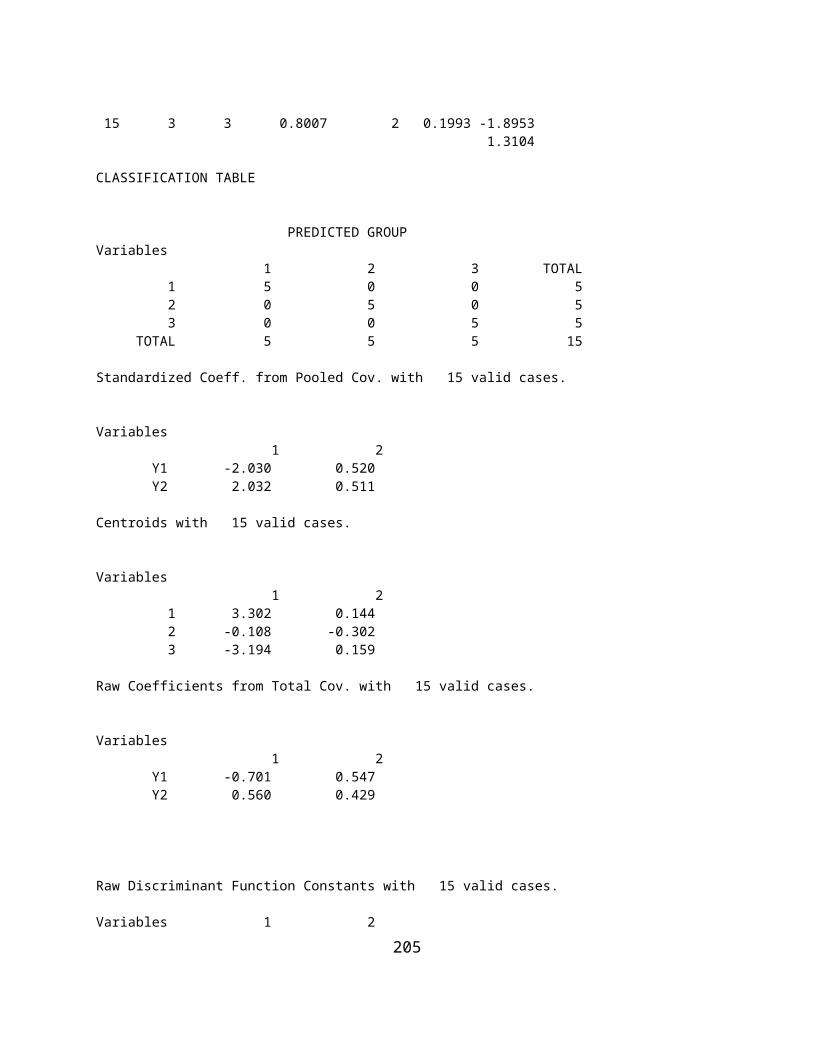
Rep1 150.000 1 Rep2 312.500 1 Rep3 529.000 1 C1R1 80.083 1 R1R1 0.167 1 R2R1 2.000 1 R3R1 6.250 1 R1C1 4.167 1 R2C1 0.889 1 R3C1 7.111 1 R1C1R1 6.000 1 R2C1R1 0.500 1 R3C1R1 6.250 1ERROR 134.667 32TOTAL 1258.000 47
TOTAL EFFECTS SUMMARY-----------------------------------------------------------SOURCE SS D.F. MS----------------------------------------------------------- Row 10.083 1 10.083 Col 8.333 1 8.333 Rep 991.500 3 330.500 Row*Col 80.083 1 80.083 Row*Rep 8.417 3 2.806 Col*Rep 12.167 3 4.056 Row*Col*Rep 12.750 3 4.250-----------------------------------------------------------
-----------------------------------------------------------SOURCE SS D.F. MS-----------------------------------------------------------BETWEEN SUBJECTS 181.000 11 Row 10.083 1 10.083 Col 8.333 1 8.333 Row*Col 80.083 1 80.083ERROR BETWEEN 82.500 8 10.312
-----------------------------------------------------------WITHIN SUBJECTS 1077.000 36 Rep 991.500 3 330.500 Row*Rep 8.417 3 2.806 Col*Rep 12.167 3 4.056 Row*Col*Rep 12.750 3 4.250ERROR WITHIN 52.167 24 2.174
-----------------------------------------------------------TOTAL 1258.000 47-----------------------------------------------------------
A comparable analysis may be performed using the file labeled ABRData.tab. In this file, the repeated measures for each subject are entered along with the row and column codes on the same line. In the previously analyzed file, we had to code the repeated dependent values on separate lines and include a code for the subject and a code for the repeated measure. Here are the results for this analysis:
205

Figure 9.26 A x B x R ANOVA Dialog Form
----------------------------------------------------------------SOURCE DF SS MS F PROB.----------------------------------------------------------------Between Subjects 11 181.000 A Effects 1 10.083 10.083 0.978 0.352 B Effects 1 8.333 8.333 0.808 0.395 AB Effects 1 80.083 80.083 7.766 0.024 Error Between 8 82.500 10.312
Within Subjects 36 1077.000 C Replications 3 991.500 330.500 152.051 0.000 AC Effects 3 8.417 2.806 1.291 0.300 BC Effects 3 12.167 4.056 1.866 0.162 ABC Effects 3 12.750 4.250 1.955 0.148 Error Within 24 52.167 2.174----------------------------------------------------------------Total 47 1258.000----------------------------------------------------------------ABR Means Table Repeated Measures C1 C2 C3 C4 A1 B1 17.000 12.000 8.667 4.000 A1 B2 15.333 10.000 7.000 2.333 A2 B1 16.667 10.000 6.000 2.333 A2 B2 17.000 14.000 9.333 8.333
206

AB Means Table B Levels B 1 B 2 A1 10.417 8.667 A2 8.750 12.167
AC Means Table C Levels C 1 C 2 C 3 C 4 A1 16.167 11.000 7.833 3.167 A2 16.833 12.000 7.667 5.333
BC Means Table C Levels C 1 C 2 C 3 C 4 B1 16.833 11.000 7.333 3.167 B2 16.167 12.000 8.167 5.333
It may be observed that the sums of squares and mean squares for the two analyses above are identical. The analysis of variance procedure (second analysis) does give the F tests as well as means (and plots if elected) for the various variance components. What is demonstrated however is that the analysis of variance model may be completely defined using multiple regression methods. It might also be noted that one can choose NOT to include all interaction terms in the GLM procedure if there is an adequate basis for expecting such interactions to be zero. Notice that we might also have included covariates in the GLM procedure. That is, one can complete a repeated measures analysis of covariance which is not an option in the regular anova procedures!
207

Median Polish Analysis
Our example uses the file labeled “GeneChips.TEX” which is an array of cells with one observation per cell. The dialogue for the analysis appears as:
Figure 9.27 Dialog for the Median Polish Analysis
The results obtained are:
Observed DataROW COLUMNS 1 2 3 4 5 1 18.000 11.000 8.000 21.000 4.000 2 13.000 7.000 5.000 16.000 7.000 3 15.000 6.000 7.000 16.000 6.000 4 19.000 15.000 12.000 18.000 5.000
Adjusted DataMEDIAN 1 2 3 4 5 Residuals--------------------------------------------------------- 0.000 0.500 0.000 -1.250 1.750 -2.250 0.000 0.000 -0.500 0.000 -0.250 0.750 4.750 0.000 0.000 0.000 -2.500 0.250 -0.750 2.250 0.000 0.000 0.000 2.500 1.250 -2.750 -2.750 0.000 ---------------------------------------------------------Col.Resid. 0.000 0.000 0.000 0.000 0.000 Col.Median 0.000 0.000 0.000 0.000 0.000
Cumulative absolute value of Row ResidualsRow = 1 Cum.Residuals = 10.250Row = 2 Cum.Residuals = 21.750Row = 3 Cum.Residuals = 17.250Row = 4 Cum.Residuals = 10.250
Cumulative absolute value of Column ResidualsColumn = 1 Cum.Residuals = 1.000
208

Column = 2 Cum.Residuals = 1.000Column = 3 Cum.Residuals = 2.000Column = 4 Cum.Residuals = 7.000Column = 5 Cum.Residuals = 6.000
Bartlett Test of Sphericity
This test is often used to determine the degree of sphericity in a matrix. A chi-squared test is used to determine the probability of the degree of sphericity found. As an example, the “cansas.TEX” file provides a significant degree of sphericity as shown in the analysis below:
Figure 9.28 Dialog for the Bartlett Test of Sphericity
CORRELATION MATRIX
Variables weight waist pulse chins situps jumps
weight 1.000 0.870 -0.366 -0.390 -0.493 -0.226 waist 0.870 1.000 -0.353 -0.552 -0.646 -0.191 pulse -0.366 -0.353 1.000 0.151 0.225 0.035 chins -0.390 -0.552 0.151 1.000 0.696 0.496 situps -0.493 -0.646 0.225 0.696 1.000 0.669 jumps -0.226 -0.191 0.035 0.496 0.669 1.000
Determinant = -3.873, log of determinant = 0.000
209

Chi-square = 69.067, D.F. = 15, Probability greater value = 0.0000
210

Correspondence Analysis
This procedure analyzes data such as that found in the “smokers.TEX” file and shown below:
CASES FOR FILE C:\Users\wgmiller\Projects\Data\Smokers.TEX
UNITS Group None Light Medium Heavy CASE 1 Senior_Mgr. 4 2 3 2 CASE 2 Junior_Mgr. 4 3 7 4 CASE 3 Senior_Emp. 25 10 12 4 CASE 4 Junior_Emp. 18 24 33 13 CASE 5 Secretaries 10 6 7 2
The dialog for the analysis appears as:
Figure 9.29 Dialog for Correspondence Analysis
The results obtained are:
CORRESPONDENCE ANALYSISBased on formulations of Bee-Leng LeeChapter 11 Correspondence Analysis for ViStaResults are based on the Generalized Singular Value Decompositionof P = A x D x B' where P is the relative frequencies observed,A are the left generalized singular vectors,D is a diagonal matrix of generalized singular values, andB' is the transpose of the right generalized singular vectors.NOTE: The first value and corresponding vectors are 1 and areto be ignored.An intermediate step is the regular SVD of the matrix Q = UDV'where Q = Dr^-1/2 x P x Dc^-1/2 where Dr is a diagonal matrix
211

of total row relative frequencies and Dc is a diagonal matrixof total column relative frequencies.
Chi-square Analysis ResultsNo. of Cases = 193
OBSERVED FREQUENCIES
Frequencies None Light Medium Heavy Total
Senior_Mgr. 4 2 3 2 11Junior_Mgr. 4 3 7 4 18Senior_Emp. 25 10 12 4 51Junior_Emp. 18 24 33 13 88Secretaries 10 6 7 2 25 Total 61 45 62 25 193
EXPECTED FREQUENCIES
Expected Values None Light Medium Heavy Senior_Mgr. 3.477 2.565 3.534 1.425 Junior_Mgr. 5.689 4.197 5.782 2.332 Senior_Emp. 16.119 11.891 16.383 6.606 Junior_Emp. 27.813 20.518 28.269 11.399 Secretaries 7.902 5.829 8.031 3.238
PROPORTIONS OF TOTAL N
Proportions None Light Medium Heavy Total Senior_Mgr. 0.021 0.010 0.016 0.010 0.057 Junior_Mgr. 0.021 0.016 0.036 0.021 0.093 Senior_Emp. 0.130 0.052 0.062 0.021 0.264 Junior_Emp. 0.093 0.124 0.171 0.067 0.456 Secretaries 0.052 0.031 0.036 0.010 0.130 Total 0.316 0.233 0.321 0.130 1.000
Chi-square = 16.442 with D.F. = 12. Prob. > value = 0.172
Liklihood Ratio = 16.348 with prob. > value = 0.1758
phi correlation = 0.2919
Pearson Correlation r = 0.0005
Mantel-Haenszel Test of Linear Association = 0.000 with probability > value = 0.9999
The coefficient of contingency = 0.280
Cramer's V = 0.169
212

Inertia = 0.0852
Figure 9.30 Correspondence Analysis Plot 1
Row Dimensions
(Ignore Column 1) None Light Medium Heavy Senior_Mgr. 1.000 -0.066 0.194 0.071 Junior_Mgr. 1.000 0.259 0.243 -0.034 Senior_Emp. 1.000 -0.381 0.011 -0.005 Junior_Emp. 1.000 0.233 -0.058 0.003 Secretaries 1.000 -0.201 -0.079 -0.008
Column Dimensions
(Ignore Column 1) None Light Medium Heavy None 1.000 -0.393 0.030 -0.001 Light 1.000 0.099 -0.141 0.022 Medium 1.000 0.196 -0.007 -0.026 Heavy 1.000 0.294 0.198 0.026
213

Figure 9.31 Correspondence Analysis Plot 2
Figure 9.32 Correspondence Analysis Plot 3
214
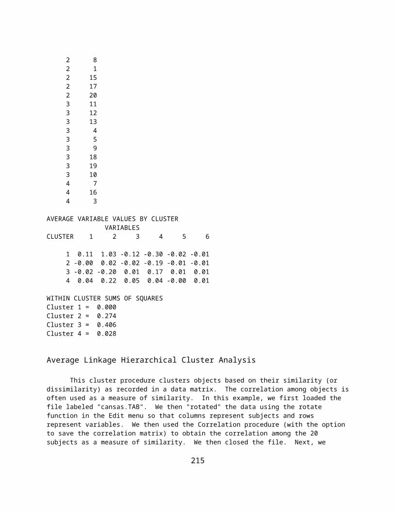
Log Linear Screening, AxB and AxBxC Analyses
The chi-squared test is often used for testing the independence of observed frequencies in a two-way table. However, there may be three classifications in which objects counted. Moreover, one may be interested in the model that best describes the observed values. OpenStat contains three procedures to analyzed cross-classified data. The first is an “over-all” screening, the second is for analyzing a two-way classification table and the third is to analyze a three-way classification table. To demonstrate these procedures, we will use a file labeled “ABCLogLinData.TEX” from the sample data files.
The Screening Procedure
Figure 9.33 Dialog for Log Linear Screening
FILE: C:\Users\wgmiller\Projects\Data\ABCLogLinData.tex
Marginal Totals for RowLevel Frequency 1 63 2 84
Marginal Totals for ColLevel Frequency 1 54 2 93
Marginal Totals for SliceLevel Frequency 1 42 2 54
215

3 51
Total Frequencies = 147
FILE: C:\Users\wgmiller\Projects\Data\ABCLogLinData.tex
EXPECTED CELL VALUES FOR MODEL OF COMPLETE INDEPENDENCE
Cell Observed Expected Log Expected 1 1 1 6 6.61 1.889 2 1 1 6 8.82 2.177 1 2 1 15 11.39 2.433 2 2 1 15 15.18 2.720 1 1 2 9 8.50 2.140 2 1 2 15 11.34 2.428 1 2 2 12 14.64 2.684 2 2 2 18 19.52 2.972 1 1 3 12 8.03 2.083 2 1 3 6 10.71 2.371 1 2 3 9 13.83 2.627 2 2 3 24 18.44 2.914Chisquare = 11.310 with probability = 0.004 (DF = 2)G squared = 11.471 with probability = 0.003 (DF = 2)
U (mu) for general loglinear model = 2.45
First Order LogLinear Model Factors and N of Cells in EachCELL U1 N Cells U2 N Cells U3 N Cells
1 1 1 -0.144 6 -0.272 6 -0.148 4 2 1 1 0.144 6 -0.272 6 -0.148 4 1 2 1 -0.144 6 0.272 6 -0.148 4 2 2 1 0.144 6 0.272 6 -0.148 4 1 1 2 -0.144 6 -0.272 6 0.103 4 2 1 2 0.144 6 -0.272 6 0.103 4 1 2 2 -0.144 6 0.272 6 0.103 4 2 2 2 0.144 6 0.272 6 0.103 4 1 1 3 -0.144 6 -0.272 6 0.046 4 2 1 3 0.144 6 -0.272 6 0.046 4 1 2 3 -0.144 6 0.272 6 0.046 4 2 2 3 0.144 6 0.272 6 0.046 4
Second Order Loglinear Model Terms and N of Cells in EachCELL U12 N Cells U13 N Cells U23 N Cells
1 1 1 -0.416 3 -0.292 2 -0.420 2 2 1 1 -0.128 3 -0.005 2 -0.420 2 1 2 1 0.128 3 -0.292 2 0.123 2 2 2 1 0.416 3 -0.005 2 0.123 2 1 1 2 -0.416 3 -0.041 2 -0.169 2 2 1 2 -0.128 3 0.247 2 -0.169 2 1 2 2 0.128 3 -0.041 2 0.375 2 2 2 2 0.416 3 0.247 2 0.375 2
216
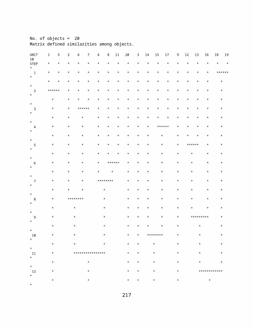
1 1 3 -0.416 3 -0.098 2 -0.226 2 2 1 3 -0.128 3 0.190 2 -0.226 2 1 2 3 0.128 3 -0.098 2 0.317 2 2 2 3 0.416 3 0.190 2 0.317 2
SCREEN FOR INTERACTIONS AMONG THE VARIABLESAdapted from the Fortran program by Lustbader and Stodola printed inApplied Statistics, Volume 30, Issue 1, 1981, pages 97-105 as AlgorithmAS 160 Partial and Marginal Association in Multidimensional Contingency Tables
Statistics for tests that the interactions of a given order are zeroORDER STATISTIC D.F. PROB. 1 15.108 4 0.004 2 6.143 5 0.293 3 5.328 2 0.070
Statistics for Marginal Association TestsVARIABLE ASSOC. PART ASSOC. MARGINAL ASSOC. D.F. PROB 1 1 3.010 3.010 1 0.083 1 2 10.472 10.472 1 0.001 1 3 1.626 1.626 2 0.444 2 1 2.224 1.773 1 0.183 2 2 1.726 1.275 2 0.529 2 3 3.095 2.644 2 0.267
The AxB Log Linear Analysis
Figure 9.34 Dialog for the A x B Log Linear Analysis
ANALYSES FOR AN I BY J CLASSIFICATION TABLE
Reference: G.J.G. Upton, The Analysis of Cross-tabulated Data, 1980
Cross-Products Odds Ratio = 1.583Log odds of the cross-products ratio = 0.460
217

Saturated Model Results
Observed FrequenciesROW/COL 1 2 TOTAL 1 27.00 36.00 63.00 2 27.00 57.00 84.00 TOTAL 54.00 93.00 147.00
Log frequencies, row average and column average of log frequenciesROW/COL 1 2 TOTAL 1 3.30 3.58 3.44 2 3.30 4.04 3.67 TOTAL 3.30 3.81 3.55
Expected FrequenciesROW/COL 1 2 TOTAL 1 27.00 36.00 63.00 2 27.00 57.00 84.00 TOTAL 54.00 93.00 147.00
Cell ParametersROW COL MU LAMBDA ROW LAMBDA COL LAMBDA ROW x COL 1 1 3.555 -0.115 -0.259 0.115 1 2 3.555 -0.115 0.259 -0.115 2 1 3.555 0.115 -0.259 -0.115 2 2 3.555 0.115 0.259 0.115
Y squared statistic for model fit = -0.000 D.F. = 0
Independent Effects Model Results
Expected FrequenciesROW/COL 1 2 TOTAL 1 23.14 39.86 63.00 2 30.86 53.14 84.00 TOTAL 54.00 93.00 147.00
Cell ParametersROW COL MU LAMBDA ROW LAMBDA COL LAMBDA ROW x COL 1 1 3.557 -0.144 -0.272 0.000 1 2 3.557 -0.144 0.272 0.000 2 1 3.557 0.144 -0.272 0.000 2 2 3.557 0.144 0.272 0.000
Y squared statistic for model fit = 1.773 D.F. = 1Chi-squared = 1.778 with 1 D.F.
No Column Effects Model Results
Expected FrequenciesROW/COL 1 2 TOTAL 1 31.50 31.50 63.00 2 42.00 42.00 84.00
218

TOTAL 73.50 73.50 147.00
Cell ParametersROW COL MU LAMBDA ROW LAMBDA COL LAMBDA ROW x COL 1 1 3.594 -0.144 0.000 -0.000 1 2 3.594 -0.144 0.000 -0.000 2 1 3.594 0.144 0.000 -0.000 2 2 3.594 0.144 0.000 -0.000
Y squared statistic for model fit = 12.245 D.F. = 2
No Row Effects Model Results
Expected FrequenciesROW/COL 1 2 TOTAL 1 27.00 46.50 73.50 2 27.00 46.50 73.50 TOTAL 54.00 93.00 147.00
Cell ParametersROW COL MU LAMBDA ROW LAMBDA COL LAMBDA ROW x COL 1 1 3.568 0.000 -0.272 0.000 1 2 3.568 0.000 0.272 0.000 2 1 3.568 0.000 -0.272 0.000 2 2 3.568 0.000 0.272 0.000
Y squared statistic for model fit = 4.783 D.F. = 2
Equiprobability Effects Model Results
Expected FrequenciesROW/COL 1 2 TOTAL 1 36.75 36.75 36.75 2 36.75 36.75 36.75 TOTAL 36.75 36.75 147.00
Cell ParametersROW COL MU LAMBDA ROW LAMBDA COL LAMBDA ROW x COL 1 1 3.604 0.000 0.000 0.000 1 2 3.604 0.000 0.000 0.000 2 1 3.604 0.000 0.000 0.000 2 2 3.604 0.000 0.000 0.000
Y squared statistic for model fit = 15.255 D.F. = 3
219

The AxBxC Log Linear Analysis
Figure 9.35 Dialog for the A x B x C Log Linear Analysis
Log-Linear Analysis of a Three Dimension Table
Observed Frequencies 1 1 1 6.000 1 1 2 9.000 1 1 3 12.000 1 2 1 15.000 1 2 2 12.000 1 2 3 9.000 2 1 1 6.000 2 1 2 15.000 2 1 3 6.000 2 2 1 15.000 2 2 2 18.000 2 2 3 24.000Totals for Dimension ARow 1 63.000Row 2 84.000Totals for Dimension BCol 1 54.000Col 2 93.000Totals for Dimension CSlice 1 42.000Slice 2 54.000Slice 3 51.000
Sub-matrix AB
ROW/COL 1 2 1 27.000 36.000 2 27.000 57.000
220

Sub-matrix AC
ROW/COL 1 2 3 1 21.000 21.000 21.000 2 21.000 33.000 30.000
Sub-matrix BC
ROW/COL 1 2 3 1 12.000 24.000 18.000 2 30.000 30.000 33.000
Saturated Model
Expected Frequencies 1 1 1 6.000 1 1 2 9.000 1 1 3 12.000 1 2 1 15.000 1 2 2 12.000 1 2 3 9.000 2 1 1 6.000 2 1 2 15.000 2 1 3 6.000 2 2 1 15.000 2 2 2 18.000 2 2 3 24.000Totals for Dimension ARow 1 63.000Row 2 84.000Totals for Dimension BCol 1 54.000Col 2 93.000Totals for Dimension CSlice 1 42.000Slice 2 54.000Slice 3 51.000
Log Frequencies 1 1 1 1.792 1 1 2 2.197 1 1 3 2.485 1 2 1 2.708 1 2 2 2.485 1 2 3 2.197 2 1 1 1.792 2 1 2 2.708 2 1 3 1.792 2 2 1 2.708 2 2 2 2.890 2 2 3 3.178Totals for Dimension ARow 1 2.311Row 2 2.511
221
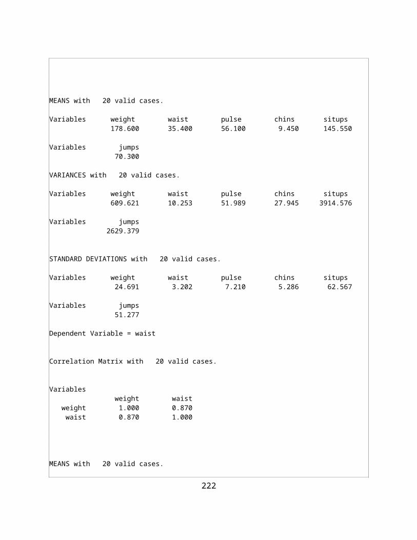
Totals for Dimension BCol 1 2.128Col 2 2.694Totals for Dimension CSlice 1 2.250Slice 2 2.570Slice 3 2.413
Cell ParametersROW COL SLICE MU LAMBDA A LAMBDA B LAMBDA C LAMBDA AB LAMBDA AC LAMBDA BC LAMBDA ABC
1 1 1 2.411 -0.100 -0.283 -0.161 0.131 0.100 -0.175 -0.131
1 1 2 2.411 -0.100 -0.283 0.159 0.131 -0.129 0.166 -0.157
1 1 3 2.411 -0.100 -0.283 0.002 0.131 0.028 0.009 0.288
1 2 1 2.411 -0.100 0.283 -0.161 -0.131 0.100 0.175 0.131
1 2 2 2.411 -0.100 0.283 0.159 -0.131 -0.129 -0.166 0.157
1 2 3 2.411 -0.100 0.283 0.002 -0.131 0.028 -0.009 -0.288
2 1 1 2.411 0.100 -0.283 -0.161 -0.131 -0.100 -0.175 0.131
2 1 2 2.411 0.100 -0.283 0.159 -0.131 0.129 0.166 0.157
2 1 3 2.411 0.100 -0.283 0.002 -0.131 -0.028 0.009 -0.288
2 2 1 2.411 0.100 0.283 -0.161 0.131 -0.100 0.175 -0.131
2 2 2 2.411 0.100 0.283 0.159 0.131 0.129 -0.166 -0.157
2 2 3 2.411 0.100 0.283 0.002 0.131 -0.028 -0.009 0.288
G squared statistic for model fit = 0.000 D.F. = 0
Model of Independence
Expected Frequencies
222

1 1 1 6.612 1 1 2 8.501 1 1 3 8.029 1 2 1 11.388 1 2 2 14.641 1 2 3 13.828 2 1 1 8.816 2 1 2 11.335 2 1 3 10.706 2 2 1 15.184 2 2 2 19.522 2 2 3 18.437Totals for Dimension ARow 1 63.000Row 2 84.000Totals for Dimension BCol 1 54.000Col 2 93.000Totals for Dimension CSlice 1 42.000Slice 2 54.000Slice 3 51.000
Log Frequencies 1 1 1 1.889 1 1 2 2.140 1 1 3 2.083 1 2 1 2.433 1 2 2 2.684 1 2 3 2.627 2 1 1 2.177 2 1 2 2.428 2 1 3 2.371 2 2 1 2.720 2 2 2 2.972 2 2 3 2.914Totals for Dimension ARow 1 2.309Row 2 2.597Totals for Dimension BCol 1 2.181Col 2 2.725Totals for Dimension CSlice 1 2.305Slice 2 2.556Slice 3 2.499
Cell ParametersROW COL SLICE MU LAMBDA A LAMBDA B LAMBDA C LAMBDA AB LAMBDA AC LAMBDA BC LAMBDA ABC
1 1 1 2.453 -0.144 -0.272 -0.148 0.000 0.000 0.000 -0.000
223

1 1 2 2.453 -0.144 -0.272 0.103 0.000 -0.000 0.000 0.000
1 1 3 2.453 -0.144 -0.272 0.046 0.000 0.000 0.000 0.000
1 2 1 2.453 -0.144 0.272 -0.148 0.000 0.000 0.000 0.000
1 2 2 2.453 -0.144 0.272 0.103 0.000 -0.000 -0.000 0.000
1 2 3 2.453 -0.144 0.272 0.046 0.000 0.000 -0.000 0.000
2 1 1 2.453 0.144 -0.272 -0.148 0.000 0.000 0.000 -0.000
2 1 2 2.453 0.144 -0.272 0.103 0.000 -0.000 0.000 0.000
2 1 3 2.453 0.144 -0.272 0.046 0.000 0.000 0.000 -0.000
2 2 1 2.453 0.144 0.272 -0.148 -0.000 0.000 0.000 0.000
2 2 2 2.453 0.144 0.272 0.103 -0.000 -0.000 -0.000 0.000
2 2 3 2.453 0.144 0.272 0.046 -0.000 0.000 -0.000 0.000
G squared statistic for model fit = 11.471 D.F. = 7
No AB Effect
Expected Frequencies 1 1 1 6.000 1 1 2 9.333 1 1 3 7.412 1 2 1 15.000 1 2 2 11.667 1 2 3 13.588 2 1 1 6.000 2 1 2 14.667 2 1 3 10.588 2 2 1 15.000 2 2 2 18.333 2 2 3 19.412Totals for Dimension ARow 1 63.000Row 2 84.000
224

Totals for Dimension BCol 1 54.000Col 2 93.000Totals for Dimension CSlice 1 42.000Slice 2 54.000Slice 3 51.000
Log Frequencies 1 1 1 1.792 1 1 2 2.234 1 1 3 2.003 1 2 1 2.708 1 2 2 2.457 1 2 3 2.609 2 1 1 1.792 2 1 2 2.686 2 1 3 2.360 2 2 1 2.708 2 2 2 2.909 2 2 3 2.966Totals for Dimension ARow 1 2.300Row 2 2.570Totals for Dimension BCol 1 2.144Col 2 2.726Totals for Dimension CSlice 1 2.250Slice 2 2.571Slice 3 2.484
Cell ParametersROW COL SLICE MU LAMBDA A LAMBDA B LAMBDA C LAMBDA AB LAMBDA AC LAMBDA BC LAMBDA ABC
1 1 1 2.435 -0.135 -0.291 -0.185 0.000 0.135 -0.167 0.000
1 1 2 2.435 -0.135 -0.291 0.136 0.000 -0.091 0.179 0.000
1 1 3 2.435 -0.135 -0.291 0.049 0.000 -0.044 -0.012 0.000
1 2 1 2.435 -0.135 0.291 -0.185 0.000 0.135 0.167 0.000
1 2 2 2.435 -0.135 0.291 0.136 0.000 -0.091 -0.179 0.000
1 2 3 2.435 -0.135 0.291 0.049 0.000 -0.044 0.012 0.000
225

2 1 1 2.435 0.135 -0.291 -0.185 0.000 -0.135 -0.167 -0.000
2 1 2 2.435 0.135 -0.291 0.136 0.000 0.091 0.179 -0.000
2 1 3 2.435 0.135 -0.291 0.049 0.000 0.044 -0.012 -0.000
2 2 1 2.435 0.135 0.291 -0.185 0.000 -0.135 0.167 0.000
2 2 2 2.435 0.135 0.291 0.136 0.000 0.091 -0.179 0.000
2 2 3 2.435 0.135 0.291 0.049 0.000 0.044 0.012 0.000
G squared statistic for model fit = 7.552 D.F. = 3No AC Effect
Expected Frequencies 1 1 1 6.000 1 1 2 12.000 1 1 3 9.000 1 2 1 11.613 1 2 2 11.613 1 2 3 12.774 2 1 1 6.000 2 1 2 12.000 2 1 3 9.000 2 2 1 18.387 2 2 2 18.387 2 2 3 20.226Totals for Dimension ARow 1 63.000Row 2 84.000Totals for Dimension BCol 1 54.000Col 2 93.000Totals for Dimension CSlice 1 42.000Slice 2 54.000Slice 3 51.000
Log Frequencies 1 1 1 1.792 1 1 2 2.485 1 1 3 2.197 1 2 1 2.452 1 2 2 2.452 1 2 3 2.547 2 1 1 1.792
226

2 1 2 2.485 2 1 3 2.197 2 2 1 2.912 2 2 2 2.912 2 2 3 3.007Totals for Dimension ARow 1 2.321Row 2 2.551Totals for Dimension BCol 1 2.158Col 2 2.714Totals for Dimension CSlice 1 2.237Slice 2 2.583Slice 3 2.487
Cell ParametersROW COL SLICE MU LAMBDA A LAMBDA B LAMBDA C LAMBDA AB LAMBDA AC LAMBDA BC LAMBDA ABC
1 1 1 2.436 -0.115 -0.278 -0.199 0.115 0.000 -0.167 0.000
1 1 2 2.436 -0.115 -0.278 0.148 0.115 0.000 0.179 0.000
1 1 3 2.436 -0.115 -0.278 0.051 0.115 -0.000 -0.012 0.000
1 2 1 2.436 -0.115 0.278 -0.199 -0.115 0.000 0.167 0.000
1 2 2 2.436 -0.115 0.278 0.148 -0.115 0.000 -0.179 0.000
1 2 3 2.436 -0.115 0.278 0.051 -0.115 -0.000 0.012 0.000
2 1 1 2.436 0.115 -0.278 -0.199 -0.115 0.000 -0.167 -0.000
2 1 2 2.436 0.115 -0.278 0.148 -0.115 0.000 0.179 -0.000
2 1 3 2.436 0.115 -0.278 0.051 -0.115 0.000 -0.012 -0.000
2 2 1 2.436 0.115 0.278 -0.199 0.115 0.000 0.167 -0.000
2 2 2 2.436 0.115 0.278 0.148 0.115 0.000 -0.179 -0.000
2 2 3 2.436 0.115 0.278 0.051
227

0.115 0.000 0.012 -0.000
G squared statistic for model fit = 7.055 D.F. = 4No BC Effect
Expected Frequencies 1 1 1 9.000 1 1 2 9.000 1 1 3 9.000 1 2 1 12.000 1 2 2 12.000 1 2 3 12.000 2 1 1 6.750 2 1 2 10.607 2 1 3 9.643 2 2 1 14.250 2 2 2 22.393 2 2 3 20.357Totals for Dimension ARow 1 63.000Row 2 84.000Totals for Dimension BCol 1 54.000Col 2 93.000Totals for Dimension CSlice 1 42.000Slice 2 54.000Slice 3 51.000
Log Frequencies 1 1 1 2.197 1 1 2 2.197 1 1 3 2.197 1 2 1 2.485 1 2 2 2.485 1 2 3 2.485 2 1 1 1.910 2 1 2 2.362 2 1 3 2.266 2 2 1 2.657 2 2 2 3.109 2 2 3 3.013Totals for Dimension ARow 1 2.341Row 2 2.553Totals for Dimension BCol 1 2.188Col 2 2.706Totals for Dimension CSlice 1 2.312Slice 2 2.538Slice 3 2.490
228

Cell ParametersROW COL SLICE MU LAMBDA A LAMBDA B LAMBDA C LAMBDA AB LAMBDA AC LAMBDA BC LAMBDA ABC
1 1 1 2.447 -0.106 -0.259 -0.135 0.115 0.135 0.000 -0.000
1 1 2 2.447 -0.106 -0.259 0.091 0.115 -0.091 0.000 -0.000
1 1 3 2.447 -0.106 -0.259 0.044 0.115 -0.044 -0.000 0.000
1 2 1 2.447 -0.106 0.259 -0.135 -0.115 0.135 -0.000 0.000
1 2 2 2.447 -0.106 0.259 0.091 -0.115 -0.091 -0.000 0.000
1 2 3 2.447 -0.106 0.259 0.044 -0.115 -0.044 -0.000 0.000
2 1 1 2.447 0.106 -0.259 -0.135 -0.115 -0.135 0.000 0.000
2 1 2 2.447 0.106 -0.259 0.091 -0.115 0.091 0.000 0.000
2 1 3 2.447 0.106 -0.259 0.044 -0.115 0.044 -0.000 0.000
2 2 1 2.447 0.106 0.259 -0.135 0.115 -0.135 -0.000 0.000
2 2 2 2.447 0.106 0.259 0.091 0.115 0.091 -0.000 0.000
2 2 3 2.447 0.106 0.259 0.044 0.115 0.044 -0.000 0.000
G squared statistic for model fit = 8.423 D.F. = 4
Model of No Slice (C) effect
Expected Frequencies 1 1 1 7.714 1 1 2 7.714 1 1 3 7.714 1 2 1 13.286 1 2 2 13.286 1 2 3 13.286 2 1 1 10.286 2 1 2 10.286
229

2 1 3 10.286 2 2 1 17.714 2 2 2 17.714 2 2 3 17.714Totals for Dimension ARow 1 63.000Row 2 84.000Totals for Dimension BCol 1 54.000Col 2 93.000Totals for Dimension CSlice 1 49.000Slice 2 49.000Slice 3 49.000
Log Frequencies 1 1 1 2.043 1 1 2 2.043 1 1 3 2.043 1 2 1 2.587 1 2 2 2.587 1 2 3 2.587 2 1 1 2.331 2 1 2 2.331 2 1 3 2.331 2 2 1 2.874 2 2 2 2.874 2 2 3 2.874Totals for Dimension ARow 1 2.315Row 2 2.603Totals for Dimension BCol 1 2.187Col 2 2.731Totals for Dimension CSlice 1 2.459Slice 2 2.459Slice 3 2.459
Cell ParametersROW COL SLICE MU LAMBDA A LAMBDA B LAMBDA C LAMBDA AB LAMBDA AC LAMBDA BC LAMBDA ABC
1 1 1 2.459 -0.144 -0.272 0.000 0.000 0.000 0.000 -0.000
1 1 2 2.459 -0.144 -0.272 0.000 0.000 0.000 0.000 -0.000
1 1 3 2.459 -0.144 -0.272 0.000 0.000 0.000 0.000 -0.000
1 2 1 2.459 -0.144 0.272 0.000 0.000 0.000 0.000 0.000
230
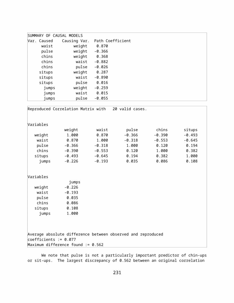
1 2 2 2.459 -0.144 0.272 0.000 0.000 0.000 0.000 0.000
1 2 3 2.459 -0.144 0.272 0.000 0.000 0.000 0.000 0.000
2 1 1 2.459 0.144 -0.272 0.000 0.000 0.000 0.000 -0.000
2 1 2 2.459 0.144 -0.272 0.000 0.000 0.000 0.000 -0.000
2 1 3 2.459 0.144 -0.272 0.000 0.000 0.000 0.000 -0.000
2 2 1 2.459 0.144 0.272 0.000 -0.000 0.000 0.000 0.000
2 2 2 2.459 0.144 0.272 0.000 -0.000 0.000 0.000 0.000
2 2 3 2.459 0.144 0.272 0.000 -0.000 0.000 0.000 0.000
G squared statistic for model fit = 13.097 D.F. = 9
Model of no Column (B) effect
Expected Frequencies 1 1 1 9.000 1 1 2 11.571 1 1 3 10.929 1 2 1 9.000 1 2 2 11.571 1 2 3 10.929 2 1 1 12.000 2 1 2 15.429 2 1 3 14.571 2 2 1 12.000 2 2 2 15.429 2 2 3 14.571Totals for Dimension ARow 1 63.000Row 2 84.000Totals for Dimension BCol 1 73.500Col 2 73.500Totals for Dimension CSlice 1 42.000Slice 2 54.000Slice 3 51.000
231

Log Frequencies 1 1 1 2.197 1 1 2 2.449 1 1 3 2.391 1 2 1 2.197 1 2 2 2.449 1 2 3 2.391 2 1 1 2.485 2 1 2 2.736 2 1 3 2.679 2 2 1 2.485 2 2 2 2.736 2 2 3 2.679Totals for Dimension ARow 1 2.346Row 2 2.633Totals for Dimension BCol 1 2.490Col 2 2.490Totals for Dimension CSlice 1 2.341Slice 2 2.592Slice 3 2.535
Cell ParametersROW COL SLICE MU LAMBDA A LAMBDA B LAMBDA C LAMBDA AB LAMBDA AC LAMBDA BC LAMBDA ABC
1 1 1 2.490 -0.144 -0.000 -0.148 0.000 0.000 0.000 -0.000
1 1 2 2.490 -0.144 -0.000 0.103 0.000 0.000 0.000 -0.000
1 1 3 2.490 -0.144 -0.000 0.046 0.000 0.000 0.000 -0.000
1 2 1 2.490 -0.144 -0.000 -0.148 0.000 0.000 0.000 -0.000
1 2 2 2.490 -0.144 -0.000 0.103 0.000 0.000 0.000 -0.000
1 2 3 2.490 -0.144 -0.000 0.046 0.000 0.000 0.000 -0.000
2 1 1 2.490 0.144 -0.000 -0.148 0.000 0.000 0.000 -0.000
2 1 2 2.490 0.144 -0.000 0.103 0.000 0.000 0.000 -0.000
2 1 3 2.490 0.144 -0.000 0.046 0.000 0.000 0.000 -0.000
232

2 2 1 2.490 0.144 -0.000 -0.148 0.000 0.000 0.000 -0.000
2 2 2 2.490 0.144 -0.000 0.103 0.000 0.000 0.000 -0.000
2 2 3 2.490 0.144 -0.000 0.046 0.000 0.000 0.000 -0.000
G squared statistic for model fit = 21.943 D.F. = 8
Model of no Row (A) effect
Expected Frequencies 1 1 1 7.714 1 1 2 9.918 1 1 3 9.367 1 2 1 13.286 1 2 2 17.082 1 2 3 16.133 2 1 1 7.714 2 1 2 9.918 2 1 3 9.367 2 2 1 13.286 2 2 2 17.082 2 2 3 16.133Totals for Dimension ARow 1 73.500Row 2 73.500Totals for Dimension BCol 1 54.000Col 2 93.000Totals for Dimension CSlice 1 42.000Slice 2 54.000Slice 3 51.000
Log Frequencies 1 1 1 2.043 1 1 2 2.294 1 1 3 2.237 1 2 1 2.587 1 2 2 2.838 1 2 3 2.781 2 1 1 2.043 2 1 2 2.294 2 1 3 2.237 2 2 1 2.587 2 2 2 2.838 2 2 3 2.781Totals for Dimension ARow 1 2.463
233

Row 2 2.463Totals for Dimension BCol 1 2.192Col 2 2.735Totals for Dimension CSlice 1 2.315Slice 2 2.566Slice 3 2.509
Cell ParametersROW COL SLICE MU LAMBDA A LAMBDA B LAMBDA C LAMBDA AB LAMBDA AC LAMBDA BC LAMBDA ABC
1 1 1 2.463 0.000 -0.272 -0.148 0.000 -0.000 0.000 0.000
1 1 2 2.463 0.000 -0.272 0.103 0.000 -0.000 0.000 0.000
1 1 3 2.463 0.000 -0.272 0.046 0.000 -0.000 0.000 0.000
1 2 1 2.463 0.000 0.272 -0.148 -0.000 -0.000 0.000 0.000
1 2 2 2.463 0.000 0.272 0.103 -0.000 -0.000 0.000 0.000
1 2 3 2.463 0.000 0.272 0.046 -0.000 -0.000 0.000 0.000
2 1 1 2.463 0.000 -0.272 -0.148 0.000 -0.000 0.000 0.000
2 1 2 2.463 0.000 -0.272 0.103 0.000 -0.000 0.000 0.000
2 1 3 2.463 0.000 -0.272 0.046 0.000 -0.000 0.000 0.000
2 2 1 2.463 0.000 0.272 -0.148 -0.000 -0.000 0.000 0.000
2 2 2 2.463 0.000 0.272 0.103 -0.000 -0.000 0.000 0.000
2 2 3 2.463 0.000 0.272 0.046 -0.000 -0.000 0.000 0.000
G squared statistic for model fit = 14.481 D.F. = 8
Equi-probability Model
234

Expected Frequencies 1 1 1 12.250 1 1 2 12.250 1 1 3 12.250 1 2 1 12.250 1 2 2 12.250 1 2 3 12.250 2 1 1 12.250 2 1 2 12.250 2 1 3 12.250 2 2 1 12.250 2 2 2 12.250 2 2 3 12.250Totals for Dimension ARow 1 73.500Row 2 73.500Totals for Dimension BCol 1 73.500Col 2 73.500Totals for Dimension CSlice 1 49.000Slice 2 49.000Slice 3 49.000
Log Frequencies 1 1 1 2.506 1 1 2 2.506 1 1 3 2.506 1 2 1 2.506 1 2 2 2.506 1 2 3 2.506 2 1 1 2.506 2 1 2 2.506 2 1 3 2.506 2 2 1 2.506 2 2 2 2.506 2 2 3 2.506Totals for Dimension ARow 1 2.506Row 2 2.506Totals for Dimension BCol 1 2.506Col 2 2.506Totals for Dimension CSlice 1 2.506Slice 2 2.506Slice 3 2.506
Cell ParametersROW COL SLICE MU LAMBDA A LAMBDA B LAMBDA C LAMBDA AB LAMBDA AC LAMBDA BC LAMBDA ABC
1 1 1 2.506 0.000 0.000 0.000 0.000 0.000 0.000 0.000
235

1 1 2 2.506 0.000 0.000 0.000 0.000 0.000 0.000 0.000
1 1 3 2.506 0.000 0.000 0.000 0.000 0.000 0.000 0.000
1 2 1 2.506 0.000 0.000 0.000 0.000 0.000 0.000 0.000
1 2 2 2.506 0.000 0.000 0.000 0.000 0.000 0.000 0.000
1 2 3 2.506 0.000 0.000 0.000 0.000 0.000 0.000 0.000
2 1 1 2.506 0.000 0.000 0.000 0.000 0.000 0.000 0.000
2 1 2 2.506 0.000 0.000 0.000 0.000 0.000 0.000 0.000
2 1 3 2.506 0.000 0.000 0.000 0.000 0.000 0.000 0.000
2 2 1 2.506 0.000 0.000 0.000 0.000 0.000 0.000 0.000
2 2 2 2.506 0.000 0.000 0.000 0.000 0.000 0.000 0.000
2 2 3 2.506 0.000 0.000 0.000 0.000 0.000 0.000 0.000
G squared statistic for model fit = 26.579 D.F. = 11
236

X. Non-Parametric
Contingency Chi-Square
Example Contingency Chi Square
In this example we will use the data file ChiData.txt which consists of two columns of data representing the row and column of a three by three contingency table. The rows represent each observation with the row and column of that observation recorded in columns one and two. We begin by selecting the Statistics / Non Parametric / Contingency Chi Square option of the menu. The following figure demonstrates that the row and column labels have been selected for the option of reading a data file containing individual cases. We have also elected all options except saving the frequency file.
Figure 10.1 Contingency Chi-Square Dialog Form
When we click the compute button, we obtain the results shown below:
Chi-square Analysis ResultsOBSERVED FREQUENCIES RowsVariables COL.1 COL.2 COL.3 COL.4 Total Row 1 5 5 5 5 20 Row 2 10 4 7 3 24 Row 3 5 10 10 2 27 Total 20 19 22 10 71
237

EXPECTED FREQUENCIES with 71 valid cases.
Variables COL.1 COL.2 COL.3 COL.4 Row 1 5.634 5.352 6.197 2.817 Row 2 6.761 6.423 7.437 3.380 Row 3 7.606 7.225 8.366 3.803
ROW PROPORTIONS with 71 valid cases.
Variables COL.1 COL.2 COL.3 COL.4 Total Row 1 0.250 0.250 0.250 0.250 1.000 Row 2 0.417 0.167 0.292 0.125 1.000 Row 3 0.185 0.370 0.370 0.074 1.000 Total 0.282 0.268 0.310 0.141 1.000
COLUMN PROPORTIONS with 71 valid cases.
Variables COL.1 COL.2 COL.3 COL.4 Total Row 1 0.250 0.263 0.227 0.500 0.282 Row 2 0.500 0.211 0.318 0.300 0.338 Row 3 0.250 0.526 0.455 0.200 0.380 Total 1.000 1.000 1.000 1.000 1.000
PROPORTIONS OF TOTAL N with 71 valid cases.
Variables COL.1 COL.2 COL.3 COL.4 Total Row 1 0.070 0.070 0.070 0.070 0.282 Row 2 0.141 0.056 0.099 0.042 0.338 Row 3 0.070 0.141 0.141 0.028 0.380 Total 0.282 0.268 0.310 0.141 1.000
CHI-SQUARED VALUE FOR CELLS with 71 valid cases.
Variables COL.1 COL.2 COL.3 COL.4 Row 1 0.071 0.023 0.231 1.692 Row 2 1.552 0.914 0.026 0.043 Row 3 0.893 1.066 0.319 0.855
Chi-square = 7.684 with D.F. = 6. Prob. > value = 0.262
It should be noted that the user has the option of reading data in three different formats. We have shown the first format where individual cases are classified by row and column. It is sometimes more convenient to record the actual frequencies in each row and cell combination. Examine the file labeled ChiSquareOne.TXT for such an example. Sometimes the investigator may only know the cell proportions and the total number of observations. In this case the third file format may be used where the proportion in each row and column combination are recorded. See the example file labeled ChiSquareTwo.TXT.
238
Spearman Rank Correlation
Example Spearman Rank Correlation
We will use the file labeled Spearman.txt for our example. The third variable represents rank data with ties. Select the Statistics / Non Parametric / Spearman Rank Correlation option from the menu. Shown below is the specification form for the analysis:
Figure 10.2 The Spearman Rank Correlation Dialog
When we click the Compute button we obtain:
Spearman Rank Correlation Between VAR2 & VAR3
Observed scores, their ranks and differences between ranks VAR2 Ranks VAR3 Ranks Rank Difference 42.00 3.00 0.00 1.50 1.50 46.00 4.00 0.00 1.50 2.50 39.00 2.00 1.00 3.50 -1.50 37.00 1.00 1.00 3.50 -2.50 65.00 8.00 3.00 5.00 3.00 88.00 11.00 4.00 6.00 5.00 86.00 10.00 5.00 7.00 3.00 56.00 6.00 6.00 8.00 -2.00 62.00 7.00 7.00 9.00 -2.00 92.00 12.00 8.00 10.50 1.50 54.00 5.00 8.00 10.50 -5.50 81.00 9.00 12.00 12.00 -3.00Spearman Rank Correlation = 0.615
t-test value for hypothesis r = 0 is 2.467
239
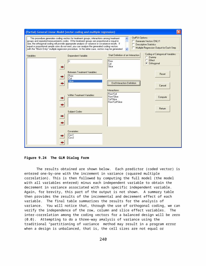
Probability > t = 0.0333
Notice that the original scores have been converted to ranks and where ties exist they have been averaged.
Mann-Whitney U Test
As an example, load the file labeled MannWhitU.txt and then select the option Statistics / Non Parametric / Mann-Whitney U Test from the menu. Shown below is the specification form in which we have indicated the analysis to perform:
Figure 10.3 The Mann=Whitney U Test Dialog Form
Upon clicking the Compute button you obtain:
Mann-Whitney U TestSee pages 116-127 in S. Siegel: Nonparametric Statistics for the Behavioral Sciences
Score Rank Group
6.00 1.50 1 6.00 1.50 2 7.00 5.00 1 7.00 5.00 1 7.00 5.00 1 7.00 5.00 1 7.00 5.00 1 8.00 9.50 1 8.00 9.50 2 8.00 9.50 2 8.00 9.50 1
240

9.00 12.00 1 10.00 16.00 1 10.00 16.00 2 10.00 16.00 2 10.00 16.00 2 10.00 16.00 1 10.00 16.00 1 10.00 16.00 1 11.00 20.50 2 11.00 20.50 2 12.00 24.50 2 12.00 24.50 2 12.00 24.50 2 12.00 24.50 2 12.00 24.50 1 12.00 24.50 1 13.00 29.50 1 13.00 29.50 2 13.00 29.50 2 13.00 29.50 2 14.00 33.00 2 14.00 33.00 2 14.00 33.00 2 15.00 36.00 2 15.00 36.00 2 15.00 36.00 2 16.00 38.00 2 17.00 39.00 2
Sum of Ranks in each GroupGroup Sum No. in Group 1 200.00 16 2 580.00 23
No. of tied rank groups = 9Statistic U = 304.0000z Statistic (corrected for ties) = 3.4262, Prob. > z = 0.0003
241
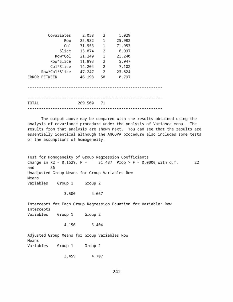
Fisher’s Exact Test
When you elect the Statistics / NonParametric / Fisher’s Exact Test option from the menu, you are shown a specification form which provides for four different formats for entering data. We have elected the last format (entry of frequencies on the form itself):
Figure 10.4 Fisher's Exact Test Dialog Form
When we click the Compute button we obtain:
Fisher Exact Probability Test
Contingency Table for Fisher Exact Test ColumnRow 1 2 1 2 8 2 4 5Probability := 0.2090
Cumulative Probability := 0.2090
Contingency Table for Fisher Exact Test ColumnRow 1 2 1 1 9 2 5 4Probability := 0.0464
Cumulative Probability := 0.2554
Contingency Table for Fisher Exact Test
242

ColumnRow 1 2 1 0 10 2 6 3Probability := 0.0031
Cumulative Probability := 0.2585
Tocher ratio computed: 0.002A random value of 0.893 selected was greater than the Tocher value.Conclusion: Accept the null Hypothesis
Notice that the probability of each combination of cell values as extreme or more extreme than that observed is computed and the probabilities summed.
Alternative formats for data files are the same as for the Contingency Chi Square analysis discussed in the previous section.
Kendall’s Coefficient of Concordance
Our example analysis will use the file labeled Concord2.txt . Load the file and select the Statistics / NonParametric / Coefficient of Concordance option. Shown below is the form completed for the analysis:
Figure 10.5 Kendal's Coefficient of Concordance
Clicking the Compute button results in the following output:
Kendall Coefficient of Concordance Analysis
Ranks Assigned to Judge Ratings of Objects
Judge 1 Objects VAR1 VAR2 VAR3 VAR4 VAR5 VAR6 VAR7 VAR8
12.0......@ࡄ 1.5000 3.5000 3.5000 5.5000 5.5000 7.0000 8.0000
243

Judge 2 Objects VAR1 VAR2 VAR3 VAR4 VAR5 VAR6 VAR7 VAR8
12.0......@ࡄ 2.0000 3.0000 4.0000 5.0000 6.0000 7.0000 8.0000
Judge 3 Objects VAR1 VAR2 VAR3 VAR4 VAR5 VAR6 VAR7 VAR8
12.0......@ࡄ 2.5000 2.5000 2.5000 6.5000 6.5000 6.5000 6.5000
Sum of Ranks for Each Object Judged Objects VAR1 VAR2 VAR3 VAR4 VAR5 VAR6 VAR7 VAR8
12.0......@ࡄ 6.0000 9.0000 10.0000 17.0000 18.0000 20.5000 22.5000
Coefficient of concordance := 0.942Average Spearman Rank Correlation := 0.913Chi-Square Statistic := 19.777Probability of a larger Chi-Square := 0.0061
If you are observing competition in the Olympics or other athletic competitions, it is fun to record the judge’s scores and examine the degree to which there is agreement among them!
Kruskal-Wallis One-Way ANOVA
As an example, load the file labeled kwanova.txt into the data grid and select the menu option for the analysis. Below is the form and the results of the analysis:
Figure 10.6 Kruskal-Wallis One Way ANOVA on Ranks Dialog
Kruskal - Wallis One-Way Analysis of Variance
244
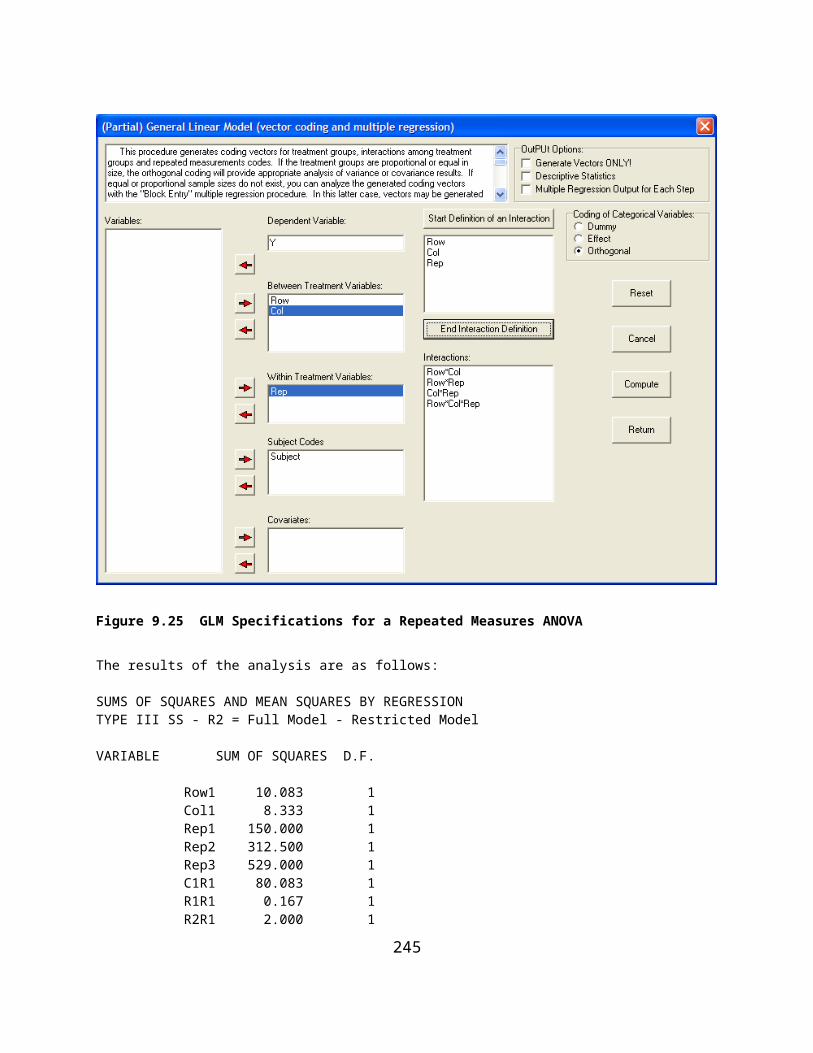
See pages 184-194 in S. Siegel: Nonparametric Statistics for the Behavioral Sciences Score Rank Group
61.00 1.00 1 82.00 2.00 2 83.00 3.00 1 96.00 4.00 1 101.00 5.00 1 109.00 6.00 2 115.00 7.00 3 124.00 8.00 2 128.00 9.00 1 132.00 10.00 2 135.00 11.00 2 147.00 12.00 3 149.00 13.00 3 166.00 14.00 3
Sum of Ranks in each GroupGroup Sum No. in Group 1 22.00 5 2 37.00 5 3 46.00 4No. of tied rank groups = 0Statisic H uncorrected for ties = 6.4057Correction for Ties = 1.0000Statistic H corrected for ties = 6.4057Corrected H is approx. chi-square with 2 D.F. and probability = 0.0406
245

Wilcoxon Matched-Pairs Signed Ranks Test
Our example uses the file labeled Wilcoxon.txt. Load this file and select the Statistics / NonParametric / Wilcoxon Matched-Pairs Signed Ranks Test option from the menu. The specification form and results are shown below:
Figure 10.7 Wilcoxon Matched Pairs Signed Ranks Test Dialog
The Wilcoxon Matched-Pairs Signed-Ranks TestSee pages 75-83 in S. Seigel: Nonparametric Statistics for the Social Sciences
Ordered Cases with cases having 0 differences eliminated:Number of cases with absolute differences greater than 0 = 10CASE VAR1 VAR2 Difference Signed Rank 3 73.00 74.00 -1.00 -1.00 8 65.00 62.00 3.00 2.00 7 76.00 80.00 -4.00 -3.00 4 43.00 37.00 6.00 4.00 5 58.00 51.00 7.00 5.00 6 56.00 43.00 13.00 6.50 10 56.00 43.00 13.00 6.50 9 82.00 63.00 19.00 8.50 1 82.00 63.00 19.00 8.50 2 69.00 42.00 27.00 10.00
Smaller sum of ranks (T) = 4.00Approximately normal z for test statistic T = 2.395Probability (1-tailed) of greater z = 0.0083NOTE: For N < 25 use tabled values for Wilcoxon Test
246

Cochran Q Test
Load the file labeled Qtest.txt and select the Statistics / NonParametric / Cochran Q Test option from the menu. Shown below is the specification form completed for the analysis of the file data and the results obtained when you click the Compute button:
Figure 10.8 Cochran Q Test Dialog Form
Cochran Q Test for Related SamplesSee pages 161-166 in S. Siegel: Nonparametric Statistics for the Behavioral SciencesMcGraw-Hill Book Company, New York, 1956
Cochran Q Statistic = 16.667which is distributed as chi-square with 2 D.F. and probability = 0.0002
247

Sign Test
The file labeled SignTest.txt contains male and female cases in which have been matched on relevant criteria and observations have been made on a 5-point Likert-type instrument. The program will compare the two scores for each pair and assign a positive or negative difference indicator. Load the file into the data grid and select the Statistics / NonParametric / Sign Test option. Shown below is the specification form which appears and the results obtained when clicking the Compute button:
Figure 10.9 The Matched Pairs Sign Test Dialog
Results for the Sign Test
Frequency of 11 out of 17 observed + sign differences.Frequency of 3 out of 17 observed - sign differences.Frequency of 3 out of 17 observed no differences.The theoretical proportion expected for +'s or -'s is 0.5 The test is for the probability of the +'s or -'s (which ever is fewer)as small or smaller than that observed given the expected proportion.
Binary Probability of 0 = 0.0001Binary Probability of 1 = 0.0009Binary Probability of 2 = 0.0056Binary Probability of 3 = 0.0222Binomial Probability of 3 or smaller out of 14 = 0.0287
248

Friedman Two Way ANOVA
For an example analysis, load the file labeled Friedman.txt and select Statistics / NonParametric / Friedman Two Way ANOVA from the menu. The data represent four treatments or repeated measures for three groups, each containing one subject. Shown below is the specification form and the results following a click of the Compute button:
Figure 10.10 The Friedman Two-Way ANOVA Dialog
FRIEDMAN TWO-WAY ANOVA ON RANKSSee pages 166-173 in S. Siegel's Nonparametric Statisticsfor the Behavioral Sciences, McGraw-Hill Book Co., New York, 1956
Treatment means - values to be ranked. with 3 valid cases.
Variables Cond.1 Cond.2 Cond.3 Cond.4 Group 1 9.000 4.000 1.000 7.000 Group 2 6.000 5.000 2.000 8.000 Group 3 9.000 1.000 2.000 6.000
Number in each group's treatment.
GROUPVariables Cond.1 Cond.2 Cond.3 Cond.4 Group 1 1 1 1 1
249
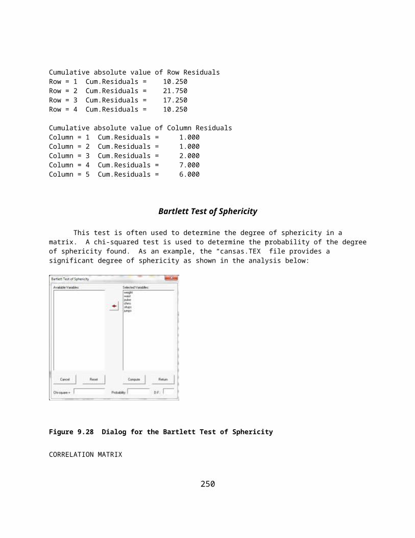
Group 2 1 1 1 1 Group 3 1 1 1 1
Score Rankings Within Groups with 3 valid cases.
Variables Cond.1 Cond.2 Cond.3 Cond.4 Group 1 4.000 2.000 1.000 3.000 Group 2 3.000 2.000 1.000 4.000 Group 3 4.000 1.000 2.000 3.000
TOTAL RANKS with 3 valid cases.
Variables Cond.1 Cond.2 Cond.3 Cond.4 11.000 5.000 4.000 10.000
Chi-square with 3 D.F. := 7.400 with probability := 0.0602Chi-square too approximate-use exact table (TABLE N)page 280-281 in Siegel
250

Probability of a Binomial Event
Select the Statistics / NonParametric / Binomial Probability option from the menu. Enter the values as shown in the specification form below and press the Compute button to obtain the shown results.
Figure 10.11 The Binomial Probability Dialog
Binomial Probability Test
Frequency of 2 out of 3 observedThe theoretical proportion expected in category A is 0.500The test is for the probability of a value in category A as small or smallerthan that observed given the expected proportion.Probability of 0 = 0.1250Probability of 1 = 0.3750Probability of 2 = 0.3750Binomial Probability of 2 or less out of 3 = 0.8750
251
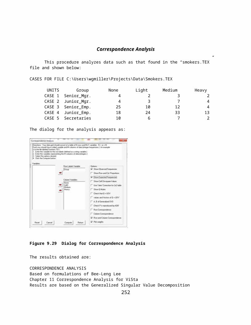
Runs Test
EXAMPLE:
The figure below shows a data set with 14 values in a file labeled "RunsTest.tab". The Runs Test option was selected from the NonParametric sub-menu under the Analyses menu. The next figure displays the dialogue box used for specifying the variable to analyze and the results of clicking the compute button.
Figure 10.12 A Sample File for the Runs Test
252

Figure 10.13 The Runs Dialog Form
253

Kendall's Tau and Partial Tau
Figure 10.14 Kendal's Tau and Partial Tau Dialog
Ranks with 12 cases.
Variables X Y Z 1 3.000 2.000 1.500 2 4.000 6.000 1.500 3 2.000 5.000 3.500 4 1.000 1.000 3.500 5 8.000 10.000 5.000 6 11.000 9.000 6.000 7 10.000 8.000 7.000 8 6.000 3.000 8.000 9 7.000 4.000 9.000 10 12.000 12.000 10.500 11 5.000 7.000 10.500 12 9.000 11.000 12.000
Kendall Tau for File: C:\Projects\Delphi\OPENSTAT\TauData.TAB
Kendall Tau for variables X and YTau = 0.6667 z = 3.017 probability > |z| = 0.001
254
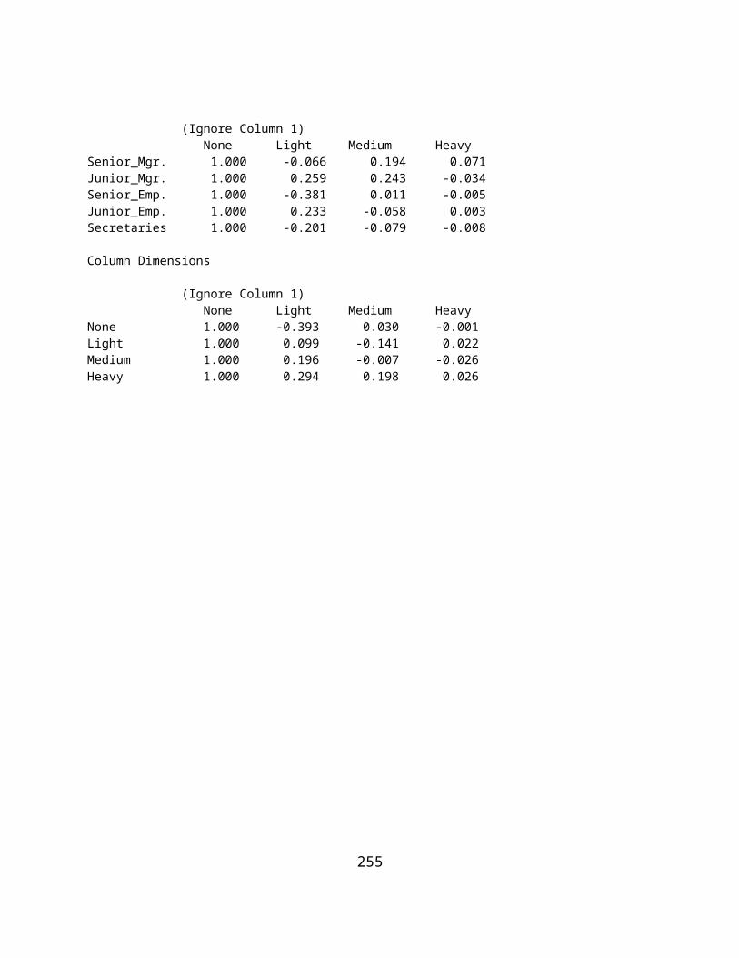
Kendall Tau for variables X and ZTau = 0.3877 z = 1.755 probability > |z| = 0.040
Kendall Tau for variables Y and ZTau = 0.3567 z = 1.614 probability > |z| = 0.053
Partial Tau = 0.6136
NOTE: Probabilities are for large N (>10)
At the time this program was written, the distribution of the Partial Tau was unknown (see Siegel 1956, page 228).
255

Kaplan-Meier Survival Test
CASES FOR FILE C:\OpenStat\KaplanMeier1.TEX
0 Time Event_Censored 1 1 2 2 3 2 3 5 2 4 6 1 5 6 1 6 6 1 7 6 1 8 6 1 9 6 1 10 8 1 11 8 1 12 9 2 13 10 1 14 10 1 15 10 2 16 12 1 17 12 1 18 12 1 19 12 1 20 12 1 21 12 1 22 12 2 23 12 2 24 13 2 25 15 2 26 15 2 27 16 2 28 16 2 29 18 2 30 18 2 31 20 1 32 20 2 33 22 2 34 24 1 35 24 1 36 24 2 37 27 2 38 28 2 39 28 2 40 28 2 41 30 1 42 30 2 43 32 1 44 33 2 45 34 2 46 36 2 47 36 2
256

48 42 1 49 44 2
We are really recording data for the "Time" variable that is sequential through the data file. We are concerned with the percent of survivors at any given time period as we progress through the observation times of the study. We record the "drop-outs" or censored subjects at each time period also. A unit cannot be censored and be one of the deaths - these are mutually exclusive.
Next we show a data file that contains both experimental and control subjects:
CASES FOR FILE C:\OpenStat\KaplanMeier2.TEX
0 Time Group Event_Censored 1 1 1 2 2 3 2 2 3 5 1 2 4 6 1 1 5 6 1 1 6 6 2 1 7 6 2 1 8 6 2 1 9 6 2 1 10 8 2 1 11 8 2 1 12 9 1 2 13 10 1 1 14 10 1 1 15 10 1 2 16 12 1 1 17 12 1 1 18 12 1 1 19 12 1 1 20 12 2 1 21 12 2 1 22 12 1 2 23 12 2 2 24 13 1 2 25 15 1 2 26 15 2 2 27 16 1 2 28 16 2 2 29 18 2 2 30 18 2 2 31 20 2 1 32 20 1 2 33 22 2 2 34 24 1 1 35 24 2 1 36 24 1 2 37 27 1 2 38 28 2 2 39 28 2 2 40 28 2 2 41 30 2 1
257

42 30 2 2 43 32 1 1 44 33 2 2 45 34 1 2 46 36 1 2 47 36 1 2 48 42 2 1 49 44 1 2
In this data we code the groups as 1 or 2. Censored cases are always coded 2 and Events are coded 1. This data is, in fact, the same data as shown in the previous data file. Note that in time period 6 there were 6 deaths (cases 4-9.) Again, notice that the time periods are in ascending order.
Shown below is the specification dialog for this second data file. This is followed by the output obtained when you click the compute button.
Figure 10.15 The Kaplan-Meier Dialog
Comparison of Two Groups Methd
TIME GROUP CENSORED TOTAL AT EVENTS AT RISK IN EXPECTED NO. AT RISK IN EXPECTED NO. RISK GROUP 1 EVENTS IN 1 GROUP 2 EVENTS IN 2 0 0 0 49 0 25 0.0000 24 0.0000 1 1 1 49 0 25 0.0000 24 0.0000 3 2 1 48 0 24 0.0000 24 0.0000 5 1 1 47 0 24 0.0000 23 0.0000 6 1 0 46 6 23 3.0000 23 3.0000 6 1 0 40 0 21 0.0000 19 0.0000 6 2 0 40 0 21 0.0000 19 0.0000 6 2 0 40 0 21 0.0000 19 0.0000 6 2 0 40 0 21 0.0000 19 0.0000 6 2 0 40 0 21 0.0000 19 0.0000 8 2 0 40 2 21 1.0500 19 0.9500 8 2 0 38 0 21 0.0000 17 0.0000 9 1 1 38 0 21 0.0000 17 0.0000 10 1 0 37 2 20 1.0811 17 0.9189 10 1 0 35 0 18 0.0000 17 0.0000 10 1 1 35 0 18 0.0000 17 0.0000 12 1 0 34 6 17 3.0000 17 3.0000 12 1 0 28 0 13 0.0000 15 0.0000
258

12 1 0 28 0 13 0.0000 15 0.0000 12 1 0 28 0 13 0.0000 15 0.0000 12 2 0 28 0 13 0.0000 15 0.0000 12 2 0 28 0 13 0.0000 15 0.0000 12 1 1 28 0 13 0.0000 15 0.0000 12 2 1 27 0 12 0.0000 15 0.0000 13 1 1 26 0 12 0.0000 14 0.0000 15 1 1 25 0 11 0.0000 14 0.0000 15 2 1 24 0 10 0.0000 14 0.0000 16 1 1 23 0 10 0.0000 13 0.0000 16 2 1 22 0 9 0.0000 13 0.0000 18 2 1 21 0 9 0.0000 12 0.0000 18 2 1 20 0 9 0.0000 11 0.0000 20 2 0 19 1 9 0.4737 10 0.5263 20 1 1 18 0 9 0.0000 9 0.0000 22 2 1 17 0 8 0.0000 9 0.0000 24 1 0 16 2 8 1.0000 8 1.0000 24 2 0 14 0 7 0.0000 7 0.0000 24 1 1 14 0 7 0.0000 7 0.0000 27 1 1 13 0 6 0.0000 7 0.0000 28 2 1 12 0 5 0.0000 7 0.0000 28 2 1 11 0 5 0.0000 6 0.0000 28 2 1 10 0 5 0.0000 5 0.0000 30 2 0 9 1 5 0.5556 4 0.4444 30 2 1 8 0 5 0.0000 3 0.0000 32 1 0 7 1 5 0.7143 2 0.2857 33 2 1 6 0 4 0.0000 2 0.0000 34 1 1 5 0 4 0.0000 1 0.0000 36 1 1 4 0 3 0.0000 1 0.0000 36 1 1 3 0 2 0.0000 1 0.0000 42 2 0 2 1 1 0.5000 1 0.5000 44 1 1 0 0 1 0.0000 0 0.0000
TIME DEATHS GROUP AT RISK PROPORTION CUMULATIVE SURVIVING PROP.SURVIVING 1 0 1 25 0.0000 1.0000 3 0 2 24 0.0000 1.0000 5 0 1 24 0.0000 1.0000 6 6 1 23 0.9130 0.9130 6 0 1 21 0.0000 0.9130 6 0 2 19 0.0000 0.8261 6 0 2 19 0.0000 0.8261 6 0 2 19 0.0000 0.8261 6 0 2 19 0.0000 0.8261 8 2 2 19 0.8947 0.7391 8 0 2 17 0.0000 0.7391 9 0 1 21 0.0000 0.9130 10 2 1 20 0.9000 0.8217 10 0 1 18 0.0000 0.8217 10 0 1 18 0.0000 0.8217 12 6 1 17 0.7647 0.6284 12 0 1 13 0.0000 0.6284 12 0 1 13 0.0000 0.6284 12 0 1 13 0.0000 0.6284 12 0 2 15 0.0000 0.6522 12 0 2 15 0.0000 0.6522 12 0 1 13 0.0000 0.6284 12 0 2 15 0.0000 0.6522 13 0 1 12 0.0000 0.6284 15 0 1 11 0.0000 0.6284 15 0 2 14 0.0000 0.6522 16 0 1 10 0.0000 0.6284 16 0 2 13 0.0000 0.6522 18 0 2 12 0.0000 0.6522 18 0 2 11 0.0000 0.6522 20 1 2 10 0.9000 0.5870 20 0 1 9 0.0000 0.6284
259

22 0 2 9 0.0000 0.5870 24 2 1 8 0.8750 0.5498 24 0 2 7 0.0000 0.5136 24 0 1 7 0.0000 0.5498 27 0 1 6 0.0000 0.5498 28 0 2 7 0.0000 0.5136 28 0 2 6 0.0000 0.5136 28 0 2 5 0.0000 0.5136 30 1 2 4 0.7500 0.3852 30 0 2 3 0.0000 0.3852 32 1 1 5 0.8000 0.4399 33 0 2 2 0.0000 0.3852 34 0 1 4 0.0000 0.4399 36 0 1 3 0.0000 0.4399 36 0 1 2 0.0000 0.4399 42 1 2 1 0.0000 0.0000 44 0 1 1 0.0000 0.4399
Total Expected Events for Experimental Group = 11.375Observed Events for Experimental Group = 10.000Total Expected Events for Control Group = 10.625Observed Events for Control Group = 12.000Chisquare = 0.344 with probability = 0.442Risk = 0.778, Log Risk = -0.250, Std.Err. Log Risk = 0.42795 Percent Confidence interval for Log Risk = (-1.087,0.586)95 Percent Confidence interval for Risk = (0.337,1.796)
EXPERIMENTAL GROUP CUMULATIVE PROBABILITYCASE TIME DEATHS CENSORED CUM.PROB. 1 1 0 1 1.000 3 5 0 1 1.000 4 6 6 0 0.913 5 6 0 0 0.913 12 9 0 1 0.913 13 10 2 0 0.822 14 10 0 0 0.822 15 10 0 1 0.822 16 12 6 0 0.628 17 12 0 0 0.628 18 12 0 0 0.628 19 12 0 0 0.628 22 12 0 1 0.628 24 13 0 1 0.628 25 15 0 1 0.628 27 16 0 1 0.628 32 20 0 1 0.628 34 24 2 0 0.550 36 24 0 1 0.550 37 27 0 1 0.550 43 32 1 0 0.440 45 34 0 1 0.440 46 36 0 1 0.440 47 36 0 1 0.440 49 44 0 1 0.440
CONTROL GROUP CUMULATIVE PROBABILITYCASE TIME DEATHS CENSORED CUM.PROB. 2 3 0 1 1.000
260

6 6 0 0 0.826 7 6 0 0 0.826 8 6 0 0 0.826 9 6 0 0 0.826 10 8 2 0 0.739 11 8 0 0 0.739 20 12 0 0 0.652 21 12 0 0 0.652 23 12 0 1 0.652 26 15 0 1 0.652 28 16 0 1 0.652 29 18 0 1 0.652 30 18 0 1 0.652 31 20 1 0 0.587 33 22 0 1 0.587 35 24 0 0 0.514 38 28 0 1 0.514 39 28 0 1 0.514 40 28 0 1 0.514 41 30 1 0 0.385 42 30 0 1 0.385 44 33 0 1 0.385 48 42 1 0 0.000
The chi-square coefficient as well as the graph indicates no difference was found between the experimental and control group beyond what is reasonably expected through random selection from the same population.
261

Figure 10.16 Experimental and Control Curves
262

The Kolmogorov-Smirnov Test
The figure below illustrates an analysis of data collected for five values with the frequency observed for each value in a separate variable:
Figure 10.17 A Sample File for the Kolmogorov-Smirnov Test
When you elect the Kolomogorov-Smirnov option under the Nonparametric analyses option, the following dialogue appears:
263

Figure 10.18 Dialog for the Kolmogorov-Smirnov Test
You can see that we elected to enter values and frequencies and are comparing to a theoretically equal distribution of values. The results obtained are shown below:
264

Figure 10.19 Frequency Distribution Plot for the Kolmogorov-Smirnov TestKolmogorov-Smirnov TestAnalysis of variable Category FROM UP TO FREQ. PCNT CUM.FREQ. CUM.PCNT. %ILE RANK
1.00 2.00 0 0.00 0.00 0.00 0.00 2.00 3.00 1 0.10 1.00 0.10 0.05 3.00 4.00 0 0.00 1.00 0.10 0.10 4.00 5.00 5 0.50 6.00 0.60 0.35 5.00 6.00 4 0.40 10.00 1.00 0.80
Kolmogorov-Smirnov Analysis of Category and equal (rectangular) distributionObserved Mean = 4.200 for 10 cases in 5 categoriesStandard Deviation = 0.919
Kolmogorov-Smirnov Distribution ComparisonCATEGORY OBSERVED COMPARISONVALUES PROBABILITIES PROBABILITIES 1 0.000 0.200 2 0.100 0.200 3 0.000 0.200 4 0.500 0.200 5 0.400 0.200
Kolmogorov-Smirnov Distribution Comparison
265

CATEGORY OBSERVED COMPARISONVALUE CUM. PROB. CUM. PROB. 1 0.000 0.200 2 0.100 0.400 3 0.100 0.600 4 0.600 0.800 5 1.000 1.000 6 1.000 1.000
Kolmogorov-Smirnov Statistic D = 0.500 with probability > D = 0.013
The difference between the observed and theoretical comparison data would not be expected to occur by chance very often (about one in a hundred times) and one would probably reject the hypothesis that the observed distribution comes from a chance distribution (equally likely frequency in each category.)
It is constructive to compare the same observed distribution with the comparison variable and with the normal distribution variable (both are viable alternatives.)
266

XI. Measurement
The Item Analysis ProgramClassical item analysis is used to estimate the reliability of test scores obtained from measures of subjects on some attribute such as achievement, aptitude or intelligence. In classical test theory, the obtained score for an individual on items is theorized to consist of a “true score” component and an “error score” component. Errors are typically assumed to be normally distributed with a mean of zero over all the subjects measured.
Several methods are available to estimate the reliability of the measures and vary according to the assumptions made about the scores. The Kuder-Richardson estimates are based on the product-moment correlation (or covariance) among items of the observed test scores and those of a theoretical “parallel” test form. The Cronbach and Hoyt estimates utilize a treatment by subjects analysis of variance design which yields identical results to the KR#20 method when item scores are dichotomous (0 and 1) values.
When you select the Classical Item Analysis procedure you will use the following dialogue box to specify how your test is to be analyzed. If the test consists of multiple sub-tests, you may define a scale for each sub-test by specifying those items belonging to each sub-test. The procedure will need to know how to determine the correct and incorrect responses. If your data are already 0 and 1 scores, the most simple method is to simply include, as the first record in your file, a case with 1’s for each item. If your data consists of values ranging, say, between 1 and 5 corresponding to alternative choices, you will either include a first case with the correct choice values or indicate you wish to Prompt for Correct Responses (as numbers when values are numbers.) If items are to be assigned different weights, you can assign those weights by selecting the “Assign Item Weights scoring option. The scored item matrix will be printed if you elect it on the output options. Three different reliability methods are available. You can select them all if you like.
267

Figure 11.1 Classical Item Analysis Dialog
Shown below is a sample output obtained from the Classical Item Analysis procedure followed by an item characteristic curve plot for one of the items. The file used was “itemdat.LAZ”.
TEST SCORING REPORT
PERSON ID NUMBER FIRST NAME LAST NAME TEST SCORE 1 Bill Miller 5.00 2 Barb Benton 4.00 3 Tom Richards 3.00 4 Keith Thomas 2.00 5 Bob King 1.00 6 Rob Moreland 0.00 7 Sandy Landis 1.00 8 Vernil Moore 2.00 9 Dick Tyler 3.00 10 Harry Cook 4.00 11 Claude Rains 5.00 12 Clark Kent 3.00 13 Bill Clinton 3.00 14 George Bush 4.00 15 Tom Jefferson 4.00 16 Abe Lincoln 2.00Alpha Reliability Estimate for Test = 0.6004 S.E. of Measurement = 0.920Analysis of Variance for Hoyt Reliabilities
SOURCE D.F. SS MS F PROBSubjects 15 6.35 0.42 2.50 0.01Within 64 13.20 0.21Items 4 3.05 0.76 4.51 0.00Error 60 10.15 0.17Total 79 19.55
Hoyt Unadjusted Test Rel. for scale TOTAL = 0.5128 S.E. of Measurement = 0.000Hoyt Adjusted Test Rel. for scale TOTAL = 0.6004 S.E. of Measurement = 0.000Hoyt Unadjusted Item Rel. for scale TOTAL = 0.1739 S.E. of Measurement = 0.000Hoyt Adjusted Item Rel. for scale TOTAL = 0.2311 S.E. of Measurement = 0.000Item and Total Score Intercorrelations with 16 cases.
Variables
268

VAR1 VAR2 VAR3 VAR4 VAR5 VAR1 1.000 0.153 0.048 -0.048 0.255 VAR2 0.153 1.000 0.493 0.323 0.164 VAR3 0.048 0.493 1.000 0.270 0.323 VAR4 -0.048 0.323 0.270 1.000 0.221 VAR5 0.255 0.164 0.323 0.221 1.000 TOTAL 0.369 0.706 0.727 0.615 0.634
Variables TOTAL VAR1 0.369 VAR2 0.706 VAR3 0.727 VAR4 0.615 VAR5 0.634 TOTAL 1.000
Means with 16 valid cases.
Variables VAR1 VAR2 VAR3 VAR4 VAR5 0.875 0.688 0.563 0.438 0.313
Variables TOTAL 2.875
Variances with 16 valid cases.
Variables VAR1 VAR2 VAR3 VAR4 VAR5 0.117 0.229 0.263 0.263 0.229
Variables TOTAL 2.117
Standard Deviations with 16 valid cases.
Variables VAR1 VAR2 VAR3 VAR4 VAR5 0.342 0.479 0.512 0.512 0.479
Variables TOTAL 1.455 KR#20 = 0.6591 for the test with mean = 1.250 and variance = 0.733Item Mean Variance Pt.Bis.r 2 0.688 0.229 0.8538 3 0.563 0.263 0.8737KR#20 = 0.6270 for the test with mean = 1.688 and variance = 1.296Item Mean Variance Pt.Bis.r 2 0.688 0.229 0.7875 3 0.563 0.263 0.7787 4 0.438 0.263 0.7073KR#20 = 0.6310 for the test with mean = 2.000 and variance = 1.867Item Mean Variance Pt.Bis.r 2 0.688 0.229 0.7135 3 0.563 0.263 0.7619 4 0.438 0.263 0.6667 5 0.313 0.229 0.6116KR#20 = 0.6004 for the test with mean = 2.875 and variance = 2.117Item Mean Variance Pt.Bis.r 2 0.688 0.229 0.7059 3 0.563 0.263 0.7267 4 0.438 0.263 0.6149 5 0.313 0.229 0.6342 1 0.875 0.117 0.3689
269

Item and Total Score Intercorrelations with 16 cases.
Variables VAR1 VAR2 VAR3 VAR4 VAR5 VAR1 1.000 0.153 0.048 -0.048 0.255 VAR2 0.153 1.000 0.493 0.323 0.164 VAR3 0.048 0.493 1.000 0.270 0.323 VAR4 -0.048 0.323 0.270 1.000 0.221 VAR5 0.255 0.164 0.323 0.221 1.000 TOTAL 0.369 0.706 0.727 0.615 0.634
Variables TOTAL VAR1 0.369 VAR2 0.706 VAR3 0.727 VAR4 0.615 VAR5 0.634 TOTAL 1.000
Means with 16 valid cases.
Variables VAR1 VAR2 VAR3 VAR4 VAR5 0.875 0.688 0.563 0.438 0.313
Variables TOTAL 2.875
Variances with 16 valid cases.
Variables VAR1 VAR2 VAR3 VAR4 VAR5 0.117 0.229 0.263 0.263 0.229
Variables TOTAL 2.117
Standard Deviations with 16 valid cases.
Variables VAR1 VAR2 VAR3 VAR4 VAR5 0.342 0.479 0.512 0.512 0.479
Variables TOTAL 1.455 Determinant of correlation matrix = 0.5209
Multiple Correlation Coefficients for Each Variable
Variable R R2 F Prob.>F DF1 DF2 VAR1 0.327 0.107 0.330 0.852 4 11 VAR2 0.553 0.306 1.212 0.360 4 11 VAR3 0.561 0.315 1.262 0.342 4 11 VAR4 0.398 0.158 0.516 0.726 4 11 VAR5 0.436 0.190 0.646 0.641 4 11
Betas in Columns with 16 cases.
Variables VAR1 VAR2 VAR3 VAR4 VAR5 VAR1 -1.000 0.161 -0.082 -0.141 0.262 VAR2 0.207 -1.000 0.442 0.274 -0.083
270
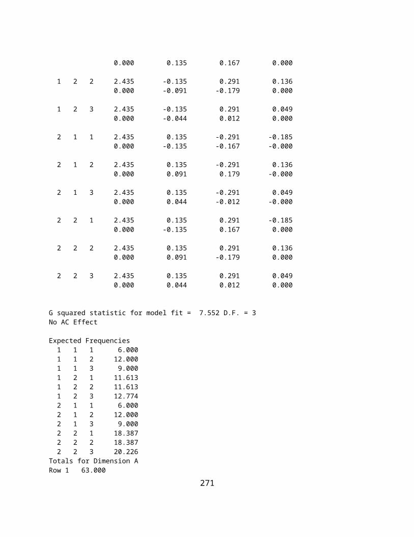
VAR3 -0.107 0.447 -1.000 0.082 0.303 VAR4 -0.149 0.226 0.067 -1.000 0.178 VAR5 0.289 -0.071 0.257 0.185 -1.000
Standard Errors of PredictionVariable Std.Error VAR1 0.377 VAR2 0.466 VAR3 0.495 VAR4 0.549 VAR5 0.503
Raw Regression Coefficients with 16 cases.
Variables VAR1 VAR2 VAR3 VAR4 VAR5 VAR1 -1.000 0.225 -0.123 -0.211 0.367 VAR2 0.147 -1.000 0.473 0.293 -0.083 VAR3 -0.071 0.418 -1.000 0.082 0.283 VAR4 -0.099 0.211 0.067 -1.000 0.167 VAR5 0.206 -0.071 0.275 0.199 -1.000
Variable Constant VAR1 0.793 VAR2 0.186 VAR3 0.230 VAR4 0.313 VAR5 -0.183
Figure 11.2 Distribution of Test Scores (Classical Analysis)
271
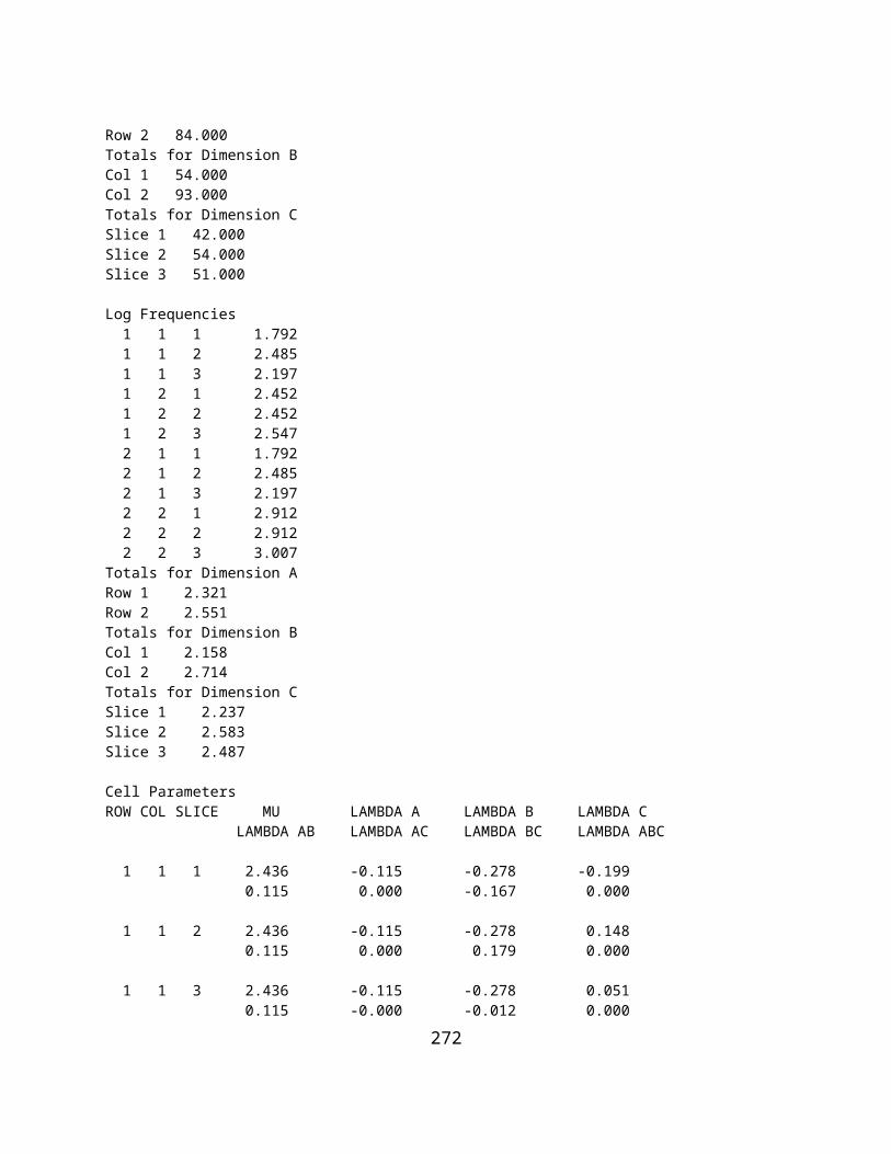
Figure 11.3 Item Means Plot
272

Analysis of Variance: Treatment by Subject and Hoyt Reliability
The Within Subjects Analysis of Variance involves the repeated measurement of the same unit of observation. These repeated observations are arranged as variables (columns) in the Main Form grid for the cases (grid rows.) If only two measures are administered, you will probably use the matched pairs (dependent) t-test method. When more than two measures are administered, you may use the repeated measures ANOVA method to test the equality of treatment level means in the population sampled. Since within subjects analysis is a part of the Hoyt Intraclass reliability estimation procedure, you may use this procedure to complete the analysis (see the Measurement procedures under the Analyses menu on the Main Form.)
Figure 11.4 Hoyt Reliability by ANOVA
The output from an example analysis is shown below:
Treatments by Subjects (AxS) ANOVA Results.
Data File = C:\lazarus\Projects\LazStats\LazStatsData\ABRDATA.LAZ
-----------------------------------------------------------SOURCE DF SS MS F Prob. > F-----------------------------------------------------------SUBJECTS 11 181.000 16.455WITHIN SUBJECTS 36 1077.000 29.917 TREATMENTS 3 991.500 330.500 127.561 0.000 RESIDUAL 33 85.500 2.591-----------------------------------------------------------TOTAL 47 1258.000 26.766-----------------------------------------------------------
TREATMENT (COLUMN) MEANS AND STANDARD DEVIATIONSVARIABLE MEAN STD.DEV.C1 16.500 2.067C2 11.500 2.431C3 7.750 2.417C4 4.250 2.864
Mean of all scores = 10.000 with standard deviation = 5.174
RELIABILITY ESTIMATES
273

TYPE OF ESTIMATE VALUEUnadjusted total reliability -0.818Unadjusted item reliability -0.127Adjusted total (Cronbach) 0.843Adjusted item reliability 0.572
BOX TEST FOR HOMOGENEITY OF VARIANCE-COVARIANCE MATRIX
SAMPLE COVARIANCE MATRIX with 12 cases.
Variables C1 C2 C3 C4 C1 4.273 2.455 1.227 1.318 C2 2.455 5.909 4.773 5.591 C3 1.227 4.773 5.841 5.432 C4 1.318 5.591 5.432 8.205
ASSUMED POP. COVARIANCE MATRIX with 12 cases.
Variables C1 C2 C3 C4 C1 6.057 0.693 0.693 0.693 C2 0.114 5.977 0.614 0.614 C3 0.114 0.103 5.914 0.551 C4 0.114 0.103 0.093 5.863
Determinant of variance-covariance matrix = 81.6Determinant of homogeneity matrix = 1.26E003ChiSquare = 108.149 with 8 degrees of freedomProbability of larger chisquare = 9.66E-007
Figure 11.5 Within Subjects ANOVA Plot
274

Kuder-Richardson #21 Reliability
The Kuder-Richardson formula #20 was developed from Classical Test Theory (true-score theory). A shorter form of the estimate can be made using only the mean, standard deviation and number of test items if one can assume that the inter-item covariances are equal. Below is the form which appears when this procedure is selected from the Measurement option of the Analyses menu:
Figure 11.6 Kuder-Richardson Formula 20 Reliability Form
Note that we have entered the maximum score (total number of items), the test mean, and the test standard deviation. When you click the Compute button, the estimate is shown in the labeled box.
275

Weighted Composite Test Reliablity
The reliability for a combination of tests, each of which has its own estimate of reliability and a weight assigned to it, may be computed. This composite will typically be greater than any one test by itself due to the likelihood that the subtests are correlated positively among themselves. Since teachers typically assign course grades based on a combination of individual tests administered over the time period of a course, this reliability estimate in built into the Grading System. See the description and examples in that section. A file labeled “CompRel.LAZ” is used in the example below:
Figure 11.7 Composite Test Reliability Dialog
Composite Test Reliability
File Analyzed: C:\lazarus\Projects\LazStats\LazStatsData\CompRel.LAZ
Correlations Among Tests with 10 cases.
Variables Test1 Test2 Test3 Test1 1.000 0.927 0.952 Test2 0.927 1.000 0.855 Test3 0.952 0.855 1.000
Means with 10 valid cases.
Variables Test1 Test2 Test3 5.500 5.500 7.500
Variances with 10 valid cases.
Variables Test1 Test2 Test3 9.167 9.167 9.167
Standard Deviations with 10 valid cases.
Variables Test1 Test2 Test3 3.028 3.028 3.028
276

Test Weights with 10 valid cases.
Variables Test1 Test2 Test3 1.000 1.000 2.000
Test Reliabilities with 10 valid cases.
Variables Test1 Test2 Test3 0.900 0.700 0.800
Composite reliability = 0.929
Rasch One Parameter Item Analysis
Item Response Theory (IRT) is another theoretical view of subject responses to items on a test. IRT suggests that items may posess one or more characteristics (parameters) that may be estimated. In the theory developed by George Rasch, one parameter, item difficulty, is estimated (in addition to the estimate of individual subject “ability” parameters.) Utilizing maximum-liklihood methods and log difficulty and log ability parameter estimates, the Rasch method attempts to estimate subject and item parameters that are “independent” of one another. This is unlike Classical theory in which the item difficulty (proportion of subects passing an item) is directly a function of the ability of the subjects sampled. IRT is sometimes also considered to be a “Latent Trait Theory” due to the assumption that all of the items are measures of the same underlying “trait”. Several tests of the “fit” of the item responses to this assumption are typically included in programs to estimate Rasch parameters. Other IRT procedures posit two or three parameters, the others being the “slope” and the “chance” parameters. The slope is the rate at which the probability of getting an item correct increases with equal units of increase in subject ability. The chance parameter is the probability of obtaining the item correct by chance alone. In the Rasch model, the chance probability is assumed to be zero and the slope parameter assumed to be equal for all items. The file labeled “itemdat.LAZ” is used for our example.
Figure 11.8 The Rasch Item Analysis Dialog
Shown below is a sample of output from a test analyzed by the Rasch model. The model cannot make ability estimates for subjects that miss all items or get all items correct so they are screened out. Parameters estimated are given in log units. Also shown is one of the item information function curve plots. Each item provides the maximum discrimination (information) at that point where the log ability of the subject is approximately the same as the log difficulty of the item. In examining the output you will note that item 1 does not appear to fit the assumptions of the Rasch model as measured by the chi-square statistic.
277

Figure 11.9 Rasch Item Log Difficulty Estimate Plot
Figure 11.10 Rasch Log Score Estimates
278

Figure 11.11 A Rasch Item Characteristic Curve
Figure 11.12 A Rasch Test Information Curve
Rasch One-Parameter Logistic Test Scaling (Item Response Theory)Written by William G. Miller
case 1 eliminated. Total score was 5Case 2 Total Score := 4 Item scores 1 1 1 1 0Case 3 Total Score := 3 Item scores 1 1 1 0 0Case 4 Total Score := 2 Item scores 1 1 0 0 0Case 5 Total Score := 1 Item scores 1 0 0 0 0case 6 eliminated. Total score was 0Case 7 Total Score := 1 Item scores 1 0 0 0 0Case 8 Total Score := 2 Item scores 1 1 0 0 0Case 9 Total Score := 3 Item scores 1 1 1 0 0Case 10 Total Score := 4 Item scores 1 1 1 1 0case 11 eliminated. Total score was 5Case 12 Total Score := 3 Item scores 1 0 1 0 1Case 13 Total Score := 3 Item scores 0 1 1 1 0Case 14 Total Score := 4 Item scores 1 1 1 0 1Case 15 Total Score := 4 Item scores 1 1 0 1 1Case 16 Total Score := 2 Item scores 1 0 0 1 0
Total number of score groups := 4
279

Matrix of Item Failures in Score Groups Score Group 1 2 3 4 TotalITEM
1 0 0 1 0 1 2 2 1 1 0 4 3 2 3 0 1 6 4 2 2 3 1 8 5 2 3 3 2 10Total 2 3 4 4 13
Item Log Odds Deviation Squared Deviation 1 -2.48 -2.13 4.54 2 -0.81 -0.46 0.21 3 -0.15 0.20 0.04 4 0.47 0.83 0.68 5 1.20 1.56 2.43Score Frequency Log Odds Freq.x Log Freq.x Log Odds Squared 1 2 -1.39 -2.77 3.84 2 3 -0.41 -1.22 0.49 3 4 0.41 1.62 0.66 4 4 1.39 5.55 7.69
Prox values and Standard Errors Item Scale Value Standard Error 1 -2.730 1.334 2 -0.584 0.770 3 0.258 0.713 4 1.058 0.731 5 1.999 0.844Y expansion factor := 1.2821
Score Scale Value Standard Error 1 -1.910 1.540 2 -0.559 1.258 3 0.559 1.258 4 1.910 1.540X expansion factor = 1.3778Maximum Likelihood Iteration Number 0Maximum Likelihood Iteration Number 1Maximum Likelihood Iteration Number 2Maximum Likelihood Iteration Number 3
Maximum Likelihood Estimates
Item Log Difficulty 1 -2.74 2 -0.64 3 0.21 4 1.04 5 1.98
Score Log Ability 1 -2.04 2 -0.54 3 0.60 4 1.92
Goodness of Fit Test for Each ItemItem Chi-Squared Degrees of ProbabilityNo. Value Freedom of Larger Value 1 29.78 9 0.0005 2 8.06 9 0.5283 3 10.42 9 0.3177 4 12.48 9 0.1875 5 9.00 9 0.4371
280

Item Data SummaryITEM PT.BIS.R. BIS.R. SLOPE PASSED FAILED RASCH DIFF 1 -0.064 -0.117 -0.12 12.00 1 -2.739 2 0.648 0.850 1.61 9.00 4 -0.644 3 0.679 0.852 1.63 7.00 6 0.207 4 0.475 0.605 0.76 5.00 8 1.038 5 0.469 0.649 0.85 3.00 10 1.981
Guttman Scalogram Analysis
Guttman scales are those measurement instruments composed of items which, ideally, form a hierarchy in which the total score of a subject can indicate the actual response (correct or incorrect) of each item. Items are arranged in order of the proportion of subjects passing the item and subjects are grouped and sequenced by their total scores. If the items measure consistently, a triangular pattern should emerge. A coefficient of “reproducibility” is obtained which may be interpreted in a manner similar to test reliability.
Dichotomously scored (0 and 1) items representing the responses of subjects in your data grid rows are the variables (grid columns) analyzed. Select the items to analyze in the same manner as you would for the Classical Item Analysis or the Rasch analysis. When you click the OK button, you will immediately be presented with the results on the output form. An example is shown below.
Figure 11.13 Guttman Scalogram Analysis Dialog
GUTTMAN SCALOGRAM ANALYSIS Cornell Method
No. of Cases := 101. No. of items := 10RESPONSE MATRIXSubject Row Item NumberLabel Sum Item 10 Item 9 Item 1 Item 3 Item 5 Item 2 0 1 0 1 0 1 0 1 0 1 0 1
1 10 0 1 0 1 0 1 0 1 0 1 0 1 6 10 0 1 0 1 0 1 0 1 0 1 0 1
20 10 0 1 0 1 0 1 0 1 0 1 0 1 46 10 0 1 0 1 0 1 0 1 0 1 0 1
281

68 10 0 1 0 1 0 1 0 1 0 1 0 1 77 10 0 1 0 1 0 1 0 1 0 1 0 1
50 9 0 1 0 1 0 1 1 0 0 1 0 1 39 9 1 0 0 1 0 1 0 1 0 1 0 1
etc.
TOTALS 53 48 52 49 51 50 51 50 50 51 48 53 ERRORS 3 22 19 9 5 20 13 10 10 10 10 13
Subject Row Item Number
Label Sum Item 8 Item 6 Item 4 Item 7 0 1 0 1 0 1 0 1
1 10 0 1 0 1 0 1 0 1 6 10 0 1 0 1 0 1 0 1 etc. 65 0 1 0 1 0 1 0 1 0 10 0 1 0 1 0 1 0 1 0
89 0 1 0 1 0 1 0 1 0
TOTALS 46 55 44 57 44 57 41 60 ERRORS 11 11 17 3 12 11 11 15
Coefficient of Reproducibility := 0.767
Successive Interval Scaling
Successive Interval Scaling was developed as an approximation of Thurstone’s Paired Comparisons method for estimation of scale values and dispersion of scale values for items designed to measure attitudes. Typically, five to nine categories are used by judges to indicate the degree to which an item expresses an attitude (if a subject agrees with the item) between very negative to very positive. Once scale values are estimated, the items responded to by subjects are scored by obtaining the median scale value of those items to which the subject agrees.
To obtain Successive interval scale values, select that option under the Measurement group in the Analyses menu on the main form. The specifications form below will appear. Select those items (variables) you wish to scale. The data analyzed consists of rows representing judges and columns representing the scale value chosen for an item by a judge. The file labeled “sucsintv.LAZ” is used as an example file.
282
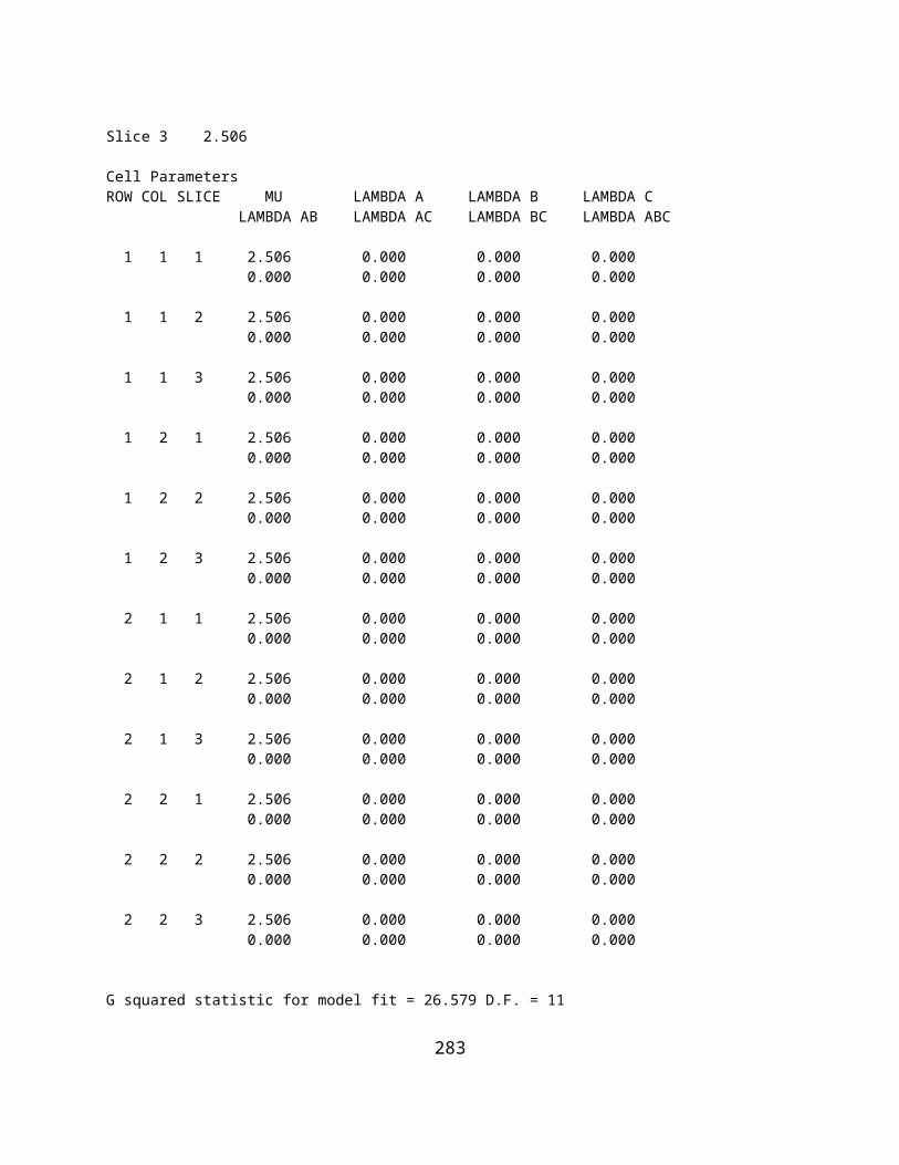
Figure 11.14 Successive Interval Scaling Dialog
When you click the OK button on the box above, the results will appear on the printout form. An example of results are presented below.
SUCCESSIVE INTERVAL SCALING RESULTS
0- 1 1- 2 2- 3 3- 4 4- 5 5- 6 6- 7 VAR1 Frequency 0 0 0 0 4 4 4Proportion 0.000 0.000 0.000 0.000 0.333 0.333 0.333Cum. Prop. 0.000 0.000 0.000 0.000 0.333 0.667 1.000Normal z - - - - -0.431 0.431 - VAR2 Frequency 0 0 1 3 4 4 0Proportion 0.000 0.000 0.083 0.250 0.333 0.333 0.000
Cum. Prop. 0.000 0.000 0.083 0.333 0.667 1.000 1.000Normal z - - -1.383 -0.431 0.431 - - VAR3 Frequency 0 0 4 3 4 1 0Proportion 0.000 0.000 0.333 0.250 0.333 0.083 0.000Cum. Prop. 0.000 0.000 0.333 0.583 0.917 1.000 1.000Normal z - - -0.431 0.210 1.383 - - VAR4 Frequency 0 3 4 5 0 0 0Proportion 0.000 0.250 0.333 0.417 0.000 0.000 0.000
Cum. Prop. 0.000 0.250 0.583 1.000 1.000 1.000 1.000Normal z - -0.674 0.210 - - - - VAR5 Frequency 5 4 3 0 0 0 0Proportion 0.417 0.333 0.250 0.000 0.000 0.000 0.000Cum. Prop. 0.417 0.750 1.000 1.000 1.000 1.000 1.000Normal z -0.210 0.674 - - - - - VAR6Frequency 1 2 2 2 2 2 1Proportion 0.083 0.167 0.167 0.167 0.167 0.167 0.083
283

Cum. Prop. 0.083 0.250 0.417 0.583 0.750 0.917 1.000Normal z -1.383 -0.674 -0.210 0.210 0.674 1.383 -
INTERVAL WIDTHS 2- 1 3- 2 4- 3 5- 4 6- 5 VAR1 - - - - 0.861 VAR2 - - 0.952 0.861 - VAR3 - - 0.641 1.173 - VAR4 - 0.885 - - - VAR5 0.885 - - - - VAR6 0.709 0.464 0.421 0.464 0.709
Mean Width 0.80 0.67 0.67 0.83 0.78No. Items 2 2 3 3 2Std. Dev.s 0.02 0.09 0.07 0.13 0.01Cum. Means 0.80 1.47 2.14 2.98 3.76
ESTIMATES OF SCALE VALUES AND THEIR DISPERSIONSItem No. Ratings Scale Value Discriminal Dispersion VAR1 12 3.368 1.224 VAR2 12 2.559 0.822 VAR3 12 1.919 0.811 VAR4 12 1.303 1.192
VAR5 12 0.199 1.192 VAR6 12 1.807 0.759
Z scores Estimated from Scale values 0- 1 1- 2 2- 3 3- 4 4- 5 5- 6 6- 7 VAR1 -3.368 -2.571 -1.897 -1.225 -0.392 0.392 VAR2 -2.559 -1.762 -1.088 -0.416 0.416 1.201 VAR3 -1.919 -1.122 -0.448 0.224 1.057 1.841 VAR4 -1.303 -0.506 0.169 0.840 1.673 2.458 VAR5 -0.199 0.598 1.272 1.943 2.776 3.000 VAR6 -1.807 -1.010 -0.336 0.336 1.168 1.953
Cumulative Theoretical Proportions 0- 1 1- 2 2- 3 3- 4 4- 5 5- 6 6- 7 VAR1 0.000 0.005 0.029 0.110 0.347 0.653 1.000 VAR2 0.005 0.039 0.138 0.339 0.661 0.885 1.000 VAR3 0.028 0.131 0.327 0.589 0.855 0.967 1.000 VAR4 0.096 0.306 0.567 0.800 0.953 0.993 1.000 VAR5 0.421 0.725 0.898 0.974 0.997 0.999 1.000 VAR6 0.035 0.156 0.369 0.631 0.879 0.975 1.000
Average Discrepency Between Theoretical and Observed Cumulative Proportions = 0.050
Maximum discrepency = 0.200 found in item VAR4
Differential Item Functioning
Anyone developing tests today should be sensitive to the fact that some test items may present a bias for one or more subgroups in the population to which the test is administered. For example, because of societal value systems, boys and girls may be exposed to quite different learning experiences during their youth. A word test in mathematics may unintentionally give an advantage to one gender group over another simply by the examples used in the item. To identify possible bias in an item, one can examine the differential item functioning of each item for the sub-groups to which the test is administered. The Mantel-Haenszel test statistic may be applied to test the difference on the item characteristic curve for the difference between a "focus" group and a "reference" group. We will demonstrate using a data set in which 40 items have been administered to 1000 subjects in one group and 1000 subjects in another group. The groups are simply coded 1 and 2 for the reference and focus groups. Since there may be very few (or no) subjects that get a specific total score, we will group the total scores obtained by subjects into
284

groups of 4 so that we are comparing subjects in the groups that have obtained total item scores of 0 to 3, 4 to 7, …, 40 to 43. As you will see, even this grouping is too small for several score groups and we should probably change the score range for the lowest and highest scores to a larger range of scores in another run.
When you elect to do this analysis, the specification form below appears:
Figure 11.15 Differential Item Functioning Dialog
On the above form you specify the items to be analyzed and also the variable defining the reference and focus group codes. You may then specify the options desired by clicking the corresponding buttons for the desired options. You also enter the number of score groups to be used in grouping the subject's total scores. When this is specified, you then enter the lowest and highest score for each of those score groups. When you have specified the low and hi score for the first group, click the right arrow on the "slider" bar to move to the next group. You will see that the lowest score has automatically been set to one higher than the previous group's highest score to save you time in entering data. You do not, of course, have to use the same size for the range of each score group. Using too large a range of scores may cut down the sensitivity of the test to differences between the groups. Fairly large samples of subjects is necessary for a reasonable analysis. Once you have completed the specifications, click the Compute button and you will see the following results are obtained (we elected to print the descriptive statistics, correlations and item plots):
Mantel-Haenszel DIF Analysis adapted by Bill Miller fromEZDIF written by Niels G. Waller
Total Means with 2000 valid cases.
Variables VAR 1 VAR 2 VAR 3 VAR 4 VAR 5 0.688 0.064 0.585 0.297 0.451
Variables VAR 6 VAR 7 VAR 8 VAR 9 VAR 10 0.806 0.217 0.827 0.960 0.568
285

Variables VAR 11 VAR 12 VAR 13 VAR 14 VAR 15 0.350 0.291 0.725 0.069 0.524
Variables VAR 16 VAR 17 VAR 18 VAR 19 VAR 20 0.350 0.943 0.545 0.017 0.985
Variables VAR 21 VAR 22 VAR 23 VAR 24 VAR 25 0.778 0.820 0.315 0.203 0.982
Variables VAR 26 VAR 27 VAR 28 VAR 29 VAR 30 0.834 0.700 0.397 0.305 0.223
Variables VAR 31 VAR 32 VAR 33 VAR 34 VAR 35 0.526 0.585 0.431 0.846 0.115
Variables VAR 36 VAR 37 VAR 38 VAR 39 VAR 40 0.150 0.817 0.909 0.793 0.329
Total Variances with 2000 valid cases.
Variables VAR 1 VAR 2 VAR 3 VAR 4 VAR 5 0.215 0.059 0.243 0.209 0.248
Variables VAR 6 VAR 7 VAR 8 VAR 9 VAR 10 0.156 0.170 0.143 0.038 0.245
Variables VAR 11 VAR 12 VAR 13 VAR 14 VAR 15 0.228 0.206 0.199 0.064 0.250
Variables VAR 16 VAR 17 VAR 18 VAR 19 VAR 20 0.228 0.054 0.248 0.017 0.015
Variables VAR 21 VAR 22 VAR 23 VAR 24 VAR 25 0.173 0.148 0.216 0.162 0.018
Variables VAR 26 VAR 27 VAR 28 VAR 29 VAR 30 0.139 0.210 0.239 0.212 0.173
Variables VAR 31 VAR 32 VAR 33 VAR 34 VAR 35 0.249 0.243 0.245 0.130 0.102
Variables VAR 36 VAR 37 VAR 38 VAR 39 VAR 40 0.128 0.150 0.083 0.164 0.221
Total Standard Deviations with 2000 valid cases.
Variables VAR 1 VAR 2 VAR 3 VAR 4 VAR 5 0.463 0.244 0.493 0.457 0.498
Variables VAR 6 VAR 7 VAR 8 VAR 9 VAR 10 0.395 0.412 0.379 0.196 0.495
Variables VAR 11 VAR 12 VAR 13 VAR 14 VAR 15 0.477 0.454 0.447 0.253 0.500
Variables VAR 16 VAR 17 VAR 18 VAR 19 VAR 20 0.477 0.233 0.498 0.129 0.124
Variables VAR 21 VAR 22 VAR 23 VAR 24 VAR 25 0.416 0.384 0.465 0.403 0.135
Variables VAR 26 VAR 27 VAR 28 VAR 29 VAR 30 0.372 0.459 0.489 0.461 0.416
Variables VAR 31 VAR 32 VAR 33 VAR 34 VAR 35 0.499 0.493 0.495 0.361 0.319
286

Variables VAR 36 VAR 37 VAR 38 VAR 39 VAR 40 0.357 0.387 0.288 0.405 0.470
Total Score: Mean = 21.318, Variance = 66.227, Std.Dev. = 8.138
Reference group size = 1000, Focus group size = 1000Correlations Among Items with 2000 cases.
Variables VAR 1 VAR 2 VAR 3 VAR 4 VAR 5 VAR 1 1.000 0.162 0.389 0.308 0.406 VAR 2 0.162 1.000 0.190 0.275 0.259 VAR 3 0.389 0.190 1.000 0.368 0.382 VAR 4 0.308 0.275 0.368 1.000 0.423 VAR 5 0.406 0.259 0.382 0.423 1.000 VAR 6 0.260 0.102 0.239 0.199 0.225 VAR 7 0.203 0.226 0.237 0.255 0.274 VAR 8 0.253 0.103 0.257 0.188 0.234 VAR 9 0.160 0.053 0.154 0.077 0.123 VAR 10 0.243 0.169 0.279 0.244 0.260 VAR 11 0.257 0.191 0.279 0.272 0.308 VAR 12 0.210 0.217 0.230 0.248 0.252 VAR 13 0.272 0.128 0.262 0.217 0.272 VAR 14 0.144 0.181 0.164 0.166 0.172 VAR 15 0.255 0.174 0.304 0.265 0.287 VAR 16 0.232 0.213 0.251 0.268 0.272 VAR 17 0.209 0.064 0.206 0.151 0.168 VAR 18 0.276 0.192 0.278 0.259 0.261 VAR 19 0.080 0.061 0.087 0.084 0.060 VAR 20 0.151 0.033 0.100 0.073 0.097 VAR 21 0.271 0.124 0.277 0.208 0.244 VAR 22 0.263 0.122 0.270 0.213 0.231 VAR 23 0.250 0.190 0.275 0.254 0.282 VAR 24 0.206 0.230 0.227 0.261 0.279 VAR 25 0.116 0.036 0.118 0.073 0.102 VAR 26 0.248 0.105 0.248 0.202 0.247 VAR 27 0.300 0.130 0.310 0.230 0.280 VAR 28 0.257 0.225 0.275 0.276 0.306 VAR 29 0.287 0.202 0.290 0.290 0.308 VAR 30 0.239 0.215 0.240 0.241 0.271 VAR 31 0.263 0.161 0.288 0.281 0.279 VAR 32 0.251 0.178 0.316 0.228 0.264 VAR 33 0.247 0.187 0.272 0.298 0.295 VAR 34 0.269 0.094 0.301 0.205 0.244 VAR 35 0.151 0.189 0.180 0.181 0.206 VAR 36 0.213 0.229 0.209 0.236 0.253 VAR 37 0.234 0.107 0.233 0.180 0.241 VAR 38 0.203 0.075 0.206 0.156 0.196 VAR 39 0.230 0.123 0.274 0.221 0.248 VAR 40 0.273 0.211 0.255 0.284 0.289
Variables VAR 6 VAR 7 VAR 8 VAR 9 VAR 10 VAR 1 0.260 0.203 0.253 0.160 0.243 VAR 2 0.102 0.226 0.103 0.053 0.169 VAR 3 0.239 0.237 0.257 0.154 0.279 VAR 4 0.199 0.255 0.188 0.077 0.244 VAR 5 0.225 0.274 0.234 0.123 0.260 VAR 6 1.000 0.196 0.267 0.217 0.281 VAR 7 0.196 1.000 0.193 0.095 0.253 VAR 8 0.267 0.193 1.000 0.189 0.285 VAR 9 0.217 0.095 0.189 1.000 0.198 VAR 10 0.281 0.253 0.285 0.198 1.000 VAR 11 0.235 0.302 0.237 0.129 0.300 VAR 12 0.202 0.229 0.198 0.103 0.268
287

VAR 13 0.308 0.202 0.256 0.177 0.299 VAR 14 0.108 0.222 0.098 0.055 0.177 VAR 15 0.268 0.278 0.264 0.163 0.335 VAR 16 0.240 0.290 0.251 0.129 0.302 VAR 17 0.238 0.114 0.261 0.224 0.201 VAR 18 0.277 0.288 0.250 0.183 0.311 VAR 19 0.055 0.118 0.060 0.027 0.076 VAR 20 0.133 0.066 0.114 0.140 0.103 VAR 21 0.308 0.202 0.299 0.167 0.306 VAR 22 0.304 0.177 0.277 0.183 0.290 VAR 23 0.253 0.322 0.217 0.111 0.326 VAR 24 0.207 0.321 0.189 0.091 0.285 VAR 25 0.224 0.063 0.192 0.086 0.135 VAR 26 0.312 0.192 0.292 0.190 0.292 VAR 27 0.284 0.247 0.299 0.156 0.320 VAR 28 0.257 0.295 0.247 0.150 0.348 VAR 29 0.248 0.320 0.206 0.108 0.293 VAR 30 0.186 0.327 0.179 0.103 0.251 VAR 31 0.273 0.281 0.261 0.169 0.323 VAR 32 0.245 0.269 0.308 0.164 0.344 VAR 33 0.284 0.291 0.234 0.147 0.336 VAR 34 0.292 0.191 0.251 0.210 0.305 VAR 35 0.157 0.232 0.149 0.074 0.204 VAR 36 0.149 0.305 0.163 0.086 0.211 VAR 37 0.338 0.183 0.271 0.167 0.240 VAR 38 0.254 0.158 0.259 0.228 0.229 VAR 39 0.282 0.197 0.278 0.236 0.278 VAR 40 0.227 0.290 0.222 0.121 0.281
Variables VAR 11 VAR 12 VAR 13 VAR 14 VAR 15 VAR 1 0.257 0.210 0.272 0.144 0.255 VAR 2 0.191 0.217 0.128 0.181 0.174 VAR 3 0.279 0.230 0.262 0.164 0.304 VAR 4 0.272 0.248 0.217 0.166 0.265 VAR 5 0.308 0.252 0.272 0.172 0.287 VAR 6 0.235 0.202 0.308 0.108 0.268 VAR 7 0.302 0.229 0.202 0.222 0.278 VAR 8 0.237 0.198 0.256 0.098 0.264 VAR 9 0.129 0.103 0.177 0.055 0.163 VAR 10 0.300 0.268 0.299 0.177 0.335 VAR 11 1.000 0.270 0.295 0.228 0.337 VAR 12 0.270 1.000 0.224 0.223 0.249 VAR 13 0.295 0.224 1.000 0.145 0.301 VAR 14 0.228 0.223 0.145 1.000 0.171 VAR 15 0.337 0.249 0.301 0.171 1.000 VAR 16 0.317 0.309 0.283 0.220 0.312 VAR 17 0.150 0.120 0.252 0.067 0.195 VAR 18 0.313 0.291 0.290 0.184 0.332 VAR 19 0.074 0.103 0.072 0.026 0.087 VAR 20 0.075 0.071 0.113 0.034 0.099 VAR 21 0.246 0.239 0.293 0.135 0.300 VAR 22 0.227 0.194 0.338 0.122 0.273 VAR 23 0.328 0.312 0.285 0.204 0.325 VAR 24 0.298 0.267 0.220 0.212 0.300 VAR 25 0.078 0.088 0.173 0.037 0.129 VAR 26 0.232 0.194 0.336 0.116 0.256 VAR 27 0.280 0.221 0.346 0.152 0.327 VAR 28 0.336 0.302 0.284 0.225 0.353 VAR 29 0.301 0.264 0.279 0.216 0.299 VAR 30 0.316 0.252 0.228 0.192 0.263 VAR 31 0.313 0.275 0.333 0.182 0.325 VAR 32 0.298 0.265 0.306 0.184 0.346 VAR 33 0.321 0.262 0.320 0.203 0.321 VAR 34 0.229 0.176 0.308 0.116 0.248 VAR 35 0.241 0.262 0.162 0.275 0.212 VAR 36 0.293 0.264 0.183 0.263 0.249
288

VAR 37 0.218 0.198 0.285 0.123 0.274 VAR 38 0.181 0.161 0.261 0.086 0.248 VAR 39 0.225 0.229 0.314 0.114 0.271 VAR 40 0.325 0.278 0.264 0.206 0.285
Variables VAR 16 VAR 17 VAR 18 VAR 19 VAR 20 VAR 1 0.232 0.209 0.276 0.080 0.151 VAR 2 0.213 0.064 0.192 0.061 0.033 VAR 3 0.251 0.206 0.278 0.087 0.100 VAR 4 0.268 0.151 0.259 0.084 0.073 VAR 5 0.272 0.168 0.261 0.060 0.097 VAR 6 0.240 0.238 0.277 0.055 0.133 VAR 7 0.290 0.114 0.288 0.118 0.066 VAR 8 0.251 0.261 0.250 0.060 0.114 VAR 9 0.129 0.224 0.183 0.027 0.140 VAR 10 0.302 0.201 0.311 0.076 0.103 VAR 11 0.317 0.150 0.313 0.074 0.075 VAR 12 0.309 0.120 0.291 0.103 0.071 VAR 13 0.283 0.252 0.290 0.072 0.113 VAR 14 0.220 0.067 0.184 0.026 0.034 VAR 15 0.312 0.195 0.332 0.087 0.099 VAR 16 1.000 0.154 0.315 0.138 0.084 VAR 17 0.154 1.000 0.193 0.032 0.230 VAR 18 0.315 0.193 1.000 0.089 0.089 VAR 19 0.138 0.032 0.089 1.000 0.017 VAR 20 0.084 0.230 0.089 0.017 1.000 VAR 21 0.244 0.245 0.305 0.061 0.128 VAR 22 0.235 0.270 0.268 0.041 0.120 VAR 23 0.348 0.158 0.334 0.102 0.085 VAR 24 0.331 0.114 0.244 0.116 0.053 VAR 25 0.085 0.157 0.136 0.018 0.133 VAR 26 0.218 0.288 0.284 0.048 0.129 VAR 27 0.278 0.241 0.302 0.069 0.112 VAR 28 0.321 0.183 0.340 0.099 0.077 VAR 29 0.356 0.145 0.306 0.115 0.083 VAR 30 0.296 0.122 0.267 0.106 0.048 VAR 31 0.325 0.166 0.319 0.094 0.084 VAR 32 0.300 0.197 0.343 0.095 0.091 VAR 33 0.293 0.185 0.299 0.120 0.101 VAR 34 0.232 0.269 0.292 0.056 0.148 VAR 35 0.274 0.089 0.231 0.050 0.045 VAR 36 0.267 0.104 0.251 0.075 0.053 VAR 37 0.199 0.200 0.259 0.062 0.119 VAR 38 0.178 0.221 0.214 0.042 0.171 VAR 39 0.235 0.192 0.276 0.067 0.126 VAR 40 0.303 0.127 0.296 0.139 0.079
Variables VAR 21 VAR 22 VAR 23 VAR 24 VAR 25 VAR 1 0.271 0.263 0.250 0.206 0.116 VAR 2 0.124 0.122 0.190 0.230 0.036 VAR 3 0.277 0.270 0.275 0.227 0.118 VAR 4 0.208 0.213 0.254 0.261 0.073 VAR 5 0.244 0.231 0.282 0.279 0.102 VAR 6 0.308 0.304 0.253 0.207 0.224 VAR 7 0.202 0.177 0.322 0.321 0.063 VAR 8 0.299 0.277 0.217 0.189 0.192 VAR 9 0.167 0.183 0.111 0.091 0.086 VAR 10 0.306 0.290 0.326 0.285 0.135 VAR 11 0.246 0.227 0.328 0.298 0.078 VAR 12 0.239 0.194 0.312 0.267 0.088 VAR 13 0.293 0.338 0.285 0.220 0.173 VAR 14 0.135 0.122 0.204 0.212 0.037 VAR 15 0.300 0.273 0.325 0.300 0.129 VAR 16 0.244 0.235 0.348 0.331 0.085
289

VAR 17 0.245 0.270 0.158 0.114 0.157 VAR 18 0.305 0.268 0.334 0.244 0.136 VAR 19 0.061 0.041 0.102 0.116 0.018 VAR 20 0.128 0.120 0.085 0.053 0.133 VAR 21 1.000 0.285 0.243 0.225 0.159 VAR 22 0.285 1.000 0.228 0.182 0.167 VAR 23 0.243 0.228 1.000 0.336 0.085 VAR 24 0.225 0.182 0.336 1.000 0.069 VAR 25 0.159 0.167 0.085 0.069 1.000 VAR 26 0.276 0.326 0.222 0.189 0.178 VAR 27 0.298 0.303 0.304 0.228 0.112 VAR 28 0.285 0.260 0.350 0.286 0.104 VAR 29 0.265 0.245 0.311 0.261 0.091 VAR 30 0.211 0.198 0.306 0.272 0.074 VAR 31 0.296 0.286 0.307 0.270 0.130 VAR 32 0.292 0.315 0.303 0.285 0.133 VAR 33 0.281 0.279 0.337 0.307 0.082 VAR 34 0.319 0.308 0.224 0.188 0.168 VAR 35 0.162 0.140 0.231 0.246 0.049 VAR 36 0.184 0.153 0.279 0.289 0.058 VAR 37 0.285 0.273 0.243 0.178 0.146 VAR 38 0.274 0.236 0.170 0.147 0.176 VAR 39 0.283 0.298 0.261 0.221 0.150 VAR 40 0.263 0.228 0.319 0.308 0.080
Variables VAR 26 VAR 27 VAR 28 VAR 29 VAR 30 VAR 1 0.248 0.300 0.257 0.287 0.239 VAR 2 0.105 0.130 0.225 0.202 0.215 VAR 3 0.248 0.310 0.275 0.290 0.240 VAR 4 0.202 0.230 0.276 0.290 0.241 VAR 5 0.247 0.280 0.306 0.308 0.271 VAR 6 0.312 0.284 0.257 0.248 0.186 VAR 7 0.192 0.247 0.295 0.320 0.327 VAR 8 0.292 0.299 0.247 0.206 0.179 VAR 9 0.190 0.156 0.150 0.108 0.103 VAR 10 0.292 0.320 0.348 0.293 0.251 VAR 11 0.232 0.280 0.336 0.301 0.316 VAR 12 0.194 0.221 0.302 0.264 0.252 VAR 13 0.336 0.346 0.284 0.279 0.228 VAR 14 0.116 0.152 0.225 0.216 0.192 VAR 15 0.256 0.327 0.353 0.299 0.263 VAR 16 0.218 0.278 0.321 0.356 0.296 VAR 17 0.288 0.241 0.183 0.145 0.122 VAR 18 0.284 0.302 0.340 0.306 0.267 VAR 19 0.048 0.069 0.099 0.115 0.106 VAR 20 0.129 0.112 0.077 0.083 0.048 VAR 21 0.276 0.298 0.285 0.265 0.211 VAR 22 0.326 0.303 0.260 0.245 0.198 VAR 23 0.222 0.304 0.350 0.311 0.306 VAR 24 0.189 0.228 0.286 0.261 0.272 VAR 25 0.178 0.112 0.104 0.091 0.074 VAR 26 1.000 0.329 0.246 0.246 0.194 VAR 27 0.329 1.000 0.311 0.306 0.244 VAR 28 0.246 0.311 1.000 0.329 0.315 VAR 29 0.246 0.306 0.329 1.000 0.269 VAR 30 0.194 0.244 0.315 0.269 1.000 VAR 31 0.269 0.305 0.298 0.322 0.289 VAR 32 0.284 0.335 0.308 0.294 0.271 VAR 33 0.283 0.302 0.328 0.333 0.297 VAR 34 0.279 0.294 0.241 0.247 0.189 VAR 35 0.123 0.188 0.236 0.272 0.236 VAR 36 0.165 0.196 0.243 0.297 0.296 VAR 37 0.307 0.271 0.251 0.241 0.163 VAR 38 0.293 0.225 0.217 0.172 0.157 VAR 39 0.287 0.310 0.285 0.247 0.202 VAR 40 0.215 0.296 0.332 0.309 0.293
290

Variables VAR 31 VAR 32 VAR 33 VAR 34 VAR 35 VAR 1 0.263 0.251 0.247 0.269 0.151 VAR 2 0.161 0.178 0.187 0.094 0.189 VAR 3 0.288 0.316 0.272 0.301 0.180 VAR 4 0.281 0.228 0.298 0.205 0.181 VAR 5 0.279 0.264 0.295 0.244 0.206 VAR 6 0.273 0.245 0.284 0.292 0.157 VAR 7 0.281 0.269 0.291 0.191 0.232 VAR 8 0.261 0.308 0.234 0.251 0.149 VAR 9 0.169 0.164 0.147 0.210 0.074 VAR 10 0.323 0.344 0.336 0.305 0.204 VAR 11 0.313 0.298 0.321 0.229 0.241 VAR 12 0.275 0.265 0.262 0.176 0.262 VAR 13 0.333 0.306 0.320 0.308 0.162 VAR 14 0.182 0.184 0.203 0.116 0.275 VAR 15 0.325 0.346 0.321 0.248 0.212 VAR 16 0.325 0.300 0.293 0.232 0.274 VAR 17 0.166 0.197 0.185 0.269 0.089 VAR 18 0.319 0.343 0.299 0.292 0.231 VAR 19 0.094 0.095 0.120 0.056 0.050 VAR 20 0.084 0.091 0.101 0.148 0.045 VAR 21 0.296 0.292 0.281 0.319 0.162 VAR 22 0.286 0.315 0.279 0.308 0.140 VAR 23 0.307 0.303 0.337 0.224 0.231 VAR 24 0.270 0.285 0.307 0.188 0.246 VAR 25 0.130 0.133 0.082 0.168 0.049 VAR 26 0.269 0.284 0.283 0.279 0.123 VAR 27 0.305 0.335 0.302 0.294 0.188 VAR 28 0.298 0.308 0.328 0.241 0.236 VAR 29 0.322 0.294 0.333 0.247 0.272 VAR 30 0.289 0.271 0.297 0.189 0.236 VAR 31 1.000 0.334 0.309 0.264 0.204 VAR 32 0.334 1.000 0.347 0.295 0.218 VAR 33 0.309 0.347 1.000 0.249 0.259 VAR 34 0.264 0.295 0.249 1.000 0.145 VAR 35 0.204 0.218 0.259 0.145 1.000 VAR 36 0.233 0.246 0.284 0.156 0.274 VAR 37 0.261 0.246 0.277 0.278 0.134 VAR 38 0.208 0.231 0.205 0.241 0.109 VAR 39 0.286 0.259 0.262 0.279 0.134 VAR 40 0.294 0.292 0.341 0.216 0.252
Variables VAR 36 VAR 37 VAR 38 VAR 39 VAR 40 VAR 1 0.213 0.234 0.203 0.230 0.273 VAR 2 0.229 0.107 0.075 0.123 0.211 VAR 3 0.209 0.233 0.206 0.274 0.255 VAR 4 0.236 0.180 0.156 0.221 0.284 VAR 5 0.253 0.241 0.196 0.248 0.289 VAR 6 0.149 0.338 0.254 0.282 0.227 VAR 7 0.305 0.183 0.158 0.197 0.290 VAR 8 0.163 0.271 0.259 0.278 0.222 VAR 9 0.086 0.167 0.228 0.236 0.121 VAR 10 0.211 0.240 0.229 0.278 0.281 VAR 11 0.293 0.218 0.181 0.225 0.325 VAR 12 0.264 0.198 0.161 0.229 0.278 VAR 13 0.183 0.285 0.261 0.314 0.264 VAR 14 0.263 0.123 0.086 0.114 0.206 VAR 15 0.249 0.274 0.248 0.271 0.285 VAR 16 0.267 0.199 0.178 0.235 0.303 VAR 17 0.104 0.200 0.221 0.192 0.127 VAR 18 0.251 0.259 0.214 0.276 0.296 VAR 19 0.075 0.062 0.042 0.067 0.139 VAR 20 0.053 0.119 0.171 0.126 0.079
291
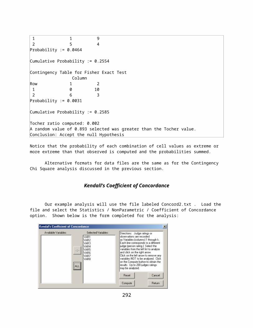
VAR 21 0.184 0.285 0.274 0.283 0.263 VAR 22 0.153 0.273 0.236 0.298 0.228 VAR 23 0.279 0.243 0.170 0.261 0.319 VAR 24 0.289 0.178 0.147 0.221 0.308 VAR 25 0.058 0.146 0.176 0.150 0.080 VAR 26 0.165 0.307 0.293 0.287 0.215 VAR 27 0.196 0.271 0.225 0.310 0.296 VAR 28 0.243 0.251 0.217 0.285 0.332 VAR 29 0.297 0.241 0.172 0.247 0.309 VAR 30 0.296 0.163 0.157 0.202 0.293 VAR 31 0.233 0.261 0.208 0.286 0.294 VAR 32 0.246 0.246 0.231 0.259 0.292 VAR 33 0.284 0.277 0.205 0.262 0.341 VAR 34 0.156 0.278 0.241 0.279 0.216 VAR 35 0.274 0.134 0.109 0.134 0.252 VAR 36 1.000 0.155 0.118 0.180 0.288 VAR 37 0.155 1.000 0.250 0.276 0.204 VAR 38 0.118 0.250 1.000 0.242 0.181 VAR 39 0.180 0.276 0.242 1.000 0.262 VAR 40 0.288 0.204 0.181 0.262 1.000 Item-Total Correlations with 2000 valid cases.
Variables VAR 1 VAR 2 VAR 3 VAR 4 VAR 5 0.527 0.352 0.556 0.514 0.563
Variables VAR 6 VAR 7 VAR 8 VAR 9 VAR 10 0.507 0.509 0.488 0.302 0.579
Variables VAR 11 VAR 12 VAR 13 VAR 14 VAR 15 0.566 0.502 0.556 0.352 0.586
Variables VAR 16 VAR 17 VAR 18 VAR 19 VAR 20 0.564 0.371 0.582 0.171 0.200
Variables VAR 21 VAR 22 VAR 23 VAR 24 VAR 25 0.532 0.511 0.574 0.511 0.235
Variables VAR 26 VAR 27 VAR 28 VAR 29 VAR 30 0.507 0.570 0.591 0.569 0.507
Variables VAR 31 VAR 32 VAR 33 VAR 34 VAR 35 0.580 0.584 0.590 0.501 0.411
Variables VAR 36 VAR 37 VAR 38 VAR 39 VAR 40 0.465 0.482 0.415 0.513 0.556 Conditioning LevelsLower Upper 1 3 4 7 8 10 11 13 14 16 17 19 20 22 23 25 26 28 29 31 32 40
292

Figure 11.16 Differential Item Function Curves
Etc.
Figure 11.17 Another ItemDifferential Functioning Curve
etc. for all items. Note the difference for the two item plots shown above! Next, the output reflects multiple passes to "fit" the data for the M-H test:
COMPUTING M-H CHI-SQUARE, PASS # 1
Cases in Reference Group
Score Level Counts by ItemVariables VAR 1 VAR 2 VAR 3 VAR 4 VAR 5 1- 3 6 6 6 6 6 4- 7 38 38 38 38 38
293

8- 10 47 47 47 47 47 11- 13 65 65 65 65 65 14- 16 101 101 101 101 101 17- 19 113 113 113 113 113 20- 22 137 137 137 137 137 23- 25 121 121 121 121 121 26- 28 114 114 114 114 114 29- 31 124 124 124 124 124 32- 40 132 132 132 132 132
Score Level Counts by ItemVariables VAR 6 VAR 7 VAR 8 VAR 9 VAR 10 1- 3 6 6 6 6 6 4- 7 38 38 38 38 38 8- 10 47 47 47 47 47 11- 13 65 65 65 65 65 14- 16 101 101 101 101 101 17- 19 113 113 113 113 113 20- 22 137 137 137 137 137 23- 25 121 121 121 121 121 26- 28 114 114 114 114 114 29- 31 124 124 124 124 124 32- 40 132 132 132 132 132
Score Level Counts by ItemVariables VAR 11 VAR 12 VAR 13 VAR 14 VAR 15 1- 3 6 6 6 6 6 4- 7 38 38 38 38 38 8- 10 47 47 47 47 47 11- 13 65 65 65 65 65 14- 16 101 101 101 101 101 17- 19 113 113 113 113 113 20- 22 137 137 137 137 137 23- 25 121 121 121 121 121 26- 28 114 114 114 114 114 29- 31 124 124 124 124 124 32- 40 132 132 132 132 132
Score Level Counts by ItemVariables VAR 16 VAR 17 VAR 18 VAR 19 VAR 20 1- 3 6 6 6 6 6 4- 7 38 38 38 38 38 8- 10 47 47 47 47 47 11- 13 65 65 65 65 65 14- 16 101 101 101 101 101 17- 19 113 113 113 113 113 20- 22 137 137 137 137 137 23- 25 121 121 121 121 121 26- 28 114 114 114 114 114 29- 31 124 124 124 124 124 32- 40 132 132 132 132 132
Score Level Counts by ItemVariables VAR 21 VAR 22 VAR 23 VAR 24 VAR 25 1- 3 6 6 6 6 6 4- 7 38 38 38 38 38 8- 10 47 47 47 47 47 11- 13 65 65 65 65 65 14- 16 101 101 101 101 101 17- 19 113 113 113 113 113
294

20- 22 137 137 137 137 137 23- 25 121 121 121 121 121 26- 28 114 114 114 114 114 29- 31 124 124 124 124 124 32- 40 132 132 132 132 132
Score Level Counts by ItemVariables VAR 26 VAR 27 VAR 28 VAR 29 VAR 30 1- 3 6 6 6 6 6 4- 7 38 38 38 38 38 8- 10 47 47 47 47 47 11- 13 65 65 65 65 65 14- 16 101 101 101 101 101 17- 19 113 113 113 113 113 20- 22 137 137 137 137 137 23- 25 121 121 121 121 121 26- 28 114 114 114 114 114 29- 31 124 124 124 124 124 32- 40 132 132 132 132 132
Score Level Counts by ItemVariables VAR 31 VAR 32 VAR 33 VAR 34 VAR 35 1- 3 6 6 6 6 6 4- 7 38 38 38 38 38 8- 10 47 47 47 47 47 11- 13 65 65 65 65 65 14- 16 101 101 101 101 101 17- 19 113 113 113 113 113 20- 22 137 137 137 137 137 23- 25 121 121 121 121 121 26- 28 114 114 114 114 114 29- 31 124 124 124 124 124 32- 40 132 132 132 132 132
Score Level Counts by ItemVariables VAR 36 VAR 37 VAR 38 VAR 39 VAR 40 1- 3 6 6 6 6 6 4- 7 38 38 38 38 38 8- 10 47 47 47 47 47 11- 13 65 65 65 65 65 14- 16 101 101 101 101 101 17- 19 113 113 113 113 113 20- 22 137 137 137 137 137 23- 25 121 121 121 121 121 26- 28 114 114 114 114 114 29- 31 124 124 124 124 124 32- 40 132 132 132 132 132
Cases in Focus Group
Score Level Counts by ItemVariables VAR 1 VAR 2 VAR 3 VAR 4 VAR 5 1- 3 7 7 7 7 7 4- 7 47 47 47 47 47 8- 10 64 64 64 64 64 11- 13 85 85 85 85 85 14- 16 123 123 123 123 123
295

17- 19 138 138 138 138 138 20- 22 127 127 127 127 127 23- 25 115 115 115 115 115 26- 28 108 108 108 108 108 29- 31 91 91 91 91 91 32- 40 95 95 95 95 95
Score Level Counts by ItemVariables VAR 6 VAR 7 VAR 8 VAR 9 VAR 10 1- 3 7 7 7 7 7 4- 7 47 47 47 47 47 8- 10 64 64 64 64 64 11- 13 85 85 85 85 85 14- 16 123 123 123 123 123 17- 19 138 138 138 138 138 20- 22 127 127 127 127 127 23- 25 115 115 115 115 115 26- 28 108 108 108 108 108 29- 31 91 91 91 91 91 32- 40 95 95 95 95 95
Score Level Counts by ItemVariables VAR 11 VAR 12 VAR 13 VAR 14 VAR 15 1- 3 7 7 7 7 7 4- 7 47 47 47 47 47 8- 10 64 64 64 64 64 11- 13 85 85 85 85 85 14- 16 123 123 123 123 123 17- 19 138 138 138 138 138 20- 22 127 127 127 127 127 23- 25 115 115 115 115 115 26- 28 108 108 108 108 108 29- 31 91 91 91 91 91 32- 40 95 95 95 95 95
Score Level Counts by ItemVariables VAR 16 VAR 17 VAR 18 VAR 19 VAR 20 1- 3 7 7 7 7 7 4- 7 47 47 47 47 47 8- 10 64 64 64 64 64 11- 13 85 85 85 85 85 14- 16 123 123 123 123 123 17- 19 138 138 138 138 138 20- 22 127 127 127 127 127 23- 25 115 115 115 115 115 26- 28 108 108 108 108 108 29- 31 91 91 91 91 91 32- 40 95 95 95 95 95
Score Level Counts by ItemVariables VAR 21 VAR 22 VAR 23 VAR 24 VAR 25 1- 3 7 7 7 7 7 4- 7 47 47 47 47 47 8- 10 64 64 64 64 64 11- 13 85 85 85 85 85 14- 16 123 123 123 123 123 17- 19 138 138 138 138 138 20- 22 127 127 127 127 127 23- 25 115 115 115 115 115 26- 28 108 108 108 108 108
296

29- 31 91 91 91 91 91 32- 40 95 95 95 95 95
Score Level Counts by ItemVariables VAR 26 VAR 27 VAR 28 VAR 29 VAR 30 1- 3 7 7 7 7 7 4- 7 47 47 47 47 47 8- 10 64 64 64 64 64 11- 13 85 85 85 85 85 14- 16 123 123 123 123 123 17- 19 138 138 138 138 138 20- 22 127 127 127 127 127 23- 25 115 115 115 115 115 26- 28 108 108 108 108 108 29- 31 91 91 91 91 91 32- 40 95 95 95 95 95
Score Level Counts by ItemVariables VAR 31 VAR 32 VAR 33 VAR 34 VAR 35 1- 3 7 7 7 7 7 4- 7 47 47 47 47 47 8- 10 64 64 64 64 64 11- 13 85 85 85 85 85 14- 16 123 123 123 123 123 17- 19 138 138 138 138 138 20- 22 127 127 127 127 127 23- 25 115 115 115 115 115 26- 28 108 108 108 108 108 29- 31 91 91 91 91 91 32- 40 95 95 95 95 95
Score Level Counts by ItemVariables VAR 36 VAR 37 VAR 38 VAR 39 VAR 40 1- 3 7 7 7 7 7 4- 7 47 47 47 47 47 8- 10 64 64 64 64 64 11- 13 85 85 85 85 85 14- 16 123 123 123 123 123 17- 19 138 138 138 138 138 20- 22 127 127 127 127 127 23- 25 115 115 115 115 115 26- 28 108 108 108 108 108 29- 31 91 91 91 91 91 32- 40 95 95 95 95 95
Insufficient data found in level: 1 - 3CODES ITEM SIG. ALPHA CHI2 P-VALUE MH D-DIF S.E. MH D-DIFC R 1 *** 9.367 283.535 0.000 -5.257 0.343C R 2 *** 8.741 65.854 0.000 -5.095 0.704C R 3 *** 7.923 287.705 0.000 -4.864 0.310C R 4 *** 10.888 305.319 0.000 -5.611 0.358C R 5 *** 13.001 399.009 0.000 -6.028 0.340B 6 *** 0.587 13.927 0.000 1.251 0.331A 7 * 0.725 5.598 0.018 0.756 0.311A 8 * 0.724 4.851 0.028 0.760 0.335B 9 * 0.506 6.230 0.013 1.599 0.620B 10 *** 0.638 15.345 0.000 1.056 0.267A 11 0.798 3.516 0.061 0.529 0.274A 12 *** 0.700 8.907 0.003 0.838 0.276A 13 *** 0.663 10.414 0.001 0.964 0.294
297

B 14 * 0.595 6.413 0.011 1.219 0.466B 15 *** 0.616 17.707 0.000 1.139 0.268B 16 *** 0.617 16.524 0.000 1.133 0.276A 17 0.850 0.355 0.551 0.382 0.537A 18 ** 0.729 7.642 0.006 0.742 0.263A 19 0.595 1.721 0.190 1.222 0.831A 20 2.004 1.805 0.179 -1.633 1.073A 21 * 0.746 4.790 0.029 0.688 0.307A 22 0.773 2.996 0.083 0.606 0.336B 23 *** 0.573 20.155 0.000 1.307 0.289A 24 * 0.736 4.796 0.029 0.722 0.320A 25 0.570 1.595 0.207 1.320 0.914B 26 *** 0.554 14.953 0.000 1.388 0.354A 27 ** 0.707 7.819 0.005 0.816 0.287A 28 * 0.750 5.862 0.015 0.675 0.272A 29 *** 0.704 7.980 0.005 0.825 0.286A 30 * 0.769 3.845 0.050 0.618 0.305A 31 ** 0.743 6.730 0.009 0.698 0.263A 32 * 0.762 5.551 0.018 0.640 0.266A 33 * 0.749 6.193 0.013 0.681 0.268A 34 0.976 0.007 1.000 0.058 0.360A 35 0.790 1.975 0.160 0.555 0.375A 36 0.832 1.310 0.252 0.432 0.354A 37 * 0.721 5.148 0.023 0.770 0.329A 38 * 0.678 4.062 0.044 0.914 0.433A 39 0.804 2.490 0.115 0.512 0.312A 40 *** 0.664 11.542 0.001 0.963 0.279
No. of items purged in pass 1 = 5Item Numbers:12345
One should probably combine the first two score groups (0-3 and 4-7) into one group and the last three groups into one group so that sufficient sample size is available for the comparisons of the two groups. This would, of course, reduce the number of groups from 11 in our original specifications to 8 score groups. The chi-square statistic identifies items you will want to give specific attention. Examine the data plots for those items. Differences found may suggest bias in those items. Only examination of the actual content can help in this decision. Even though two groups may differ in their item response patterns does not provide sufficient grounds to establish bias - perhaps it simply identifies a true difference in educational achievement due to other factors.
Adjustment of Reliability For Variance Change
Researchers will sometimes use a test that has been standardized on a large, heterogenous population of subjects. Such tests typically report rather high internal-consistency reliability estimates (e.g. Cronbach's estimate.) But what is the reliability if one administers the test to a much more homogeneous population? For example, assume a high school counselor administers a "College Aptitude Test" that reports a reliability of 0.95 with a standard deviation of 15 (variance of 225) and a mean of 20.0 for the national norm. What reliability would the counselor expect to obtain for her sample of students that obtain a mean of 22.8 and a standard deviation of 10.2 (variance of 104.04)? This procedure will help provide the estimate. Shown below is the specification form and our sample values entered. When the compute button is clicked, the results shown are obtained.
298

299

Figure 11.18 Reliability Adjustment for Variability Dialog
300

Polytomous DIF Analysis
The purpose of the differential item functioning program is to identify test or attitude items that "perform" differently for two groups - a target group and a reference group. Two procedures are provided and selected on the basis of whether the items are dichotomous (0 and 1 scoring) or consist of multiple categories (e.g. Likert responses ranging from 1 to 5.) The latter case is where the Polytomous DIF Analysis is selected. When you initiate this procedure you will see the dialogue box shown below:
Figure 11.19 Polytomous Item Differential Functioning Dialog
The results from an analysis of three items with five categories that have been collapsed into three category levels is shown below. A sample of 500 subject's attitude scores were observed.
Polytomous Item DIF Analysis adapted by Bill Miller fromProcedures for extending item bias detection techniquesby Catherine Welch and H.D. Hoover, 1993Applied Measurement in Education 6(1), pages 1-19.
Conditioning LevelsLower Upper 0 1 2 3 4 5
For Item 1:
Observed Category FrequenciesItem Group Level Category Number 1 2 3 4 5 1 Ref. 1 46 51 39 64 48 1 Focal 1 40 41 38 46 42 1 Total 1 86 92 77 110 90
1 Ref. 2 2 0 0 0 0 1 Focal 2 1 0 0 0 0 1 Total 2 3 0 0 0 0
301
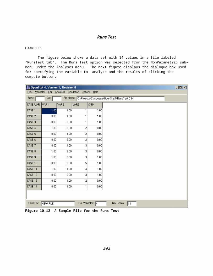
1 Ref. 3 12 8 1 0 0 1 Focal 3 15 6 0 0 0 1 Total 3 27 14 1 0 0
t-test values for Reference and Focus Means for each levelMean Reference = 3.069 SD = 24.396 N = 248Mean Focal = 3.043 SD = 21.740 N = 207Level 1 t = -0.011 with deg. freedom = 453Mean Reference = 2.000 SD = 2.000 N = 2Mean Focal = 1.000 SD = 1.000 N = 1Level 2 t = 0.000 with deg. freedom = 0Mean Reference = 1.476 SD = 4.262 N = 21Mean Focal = 1.286 SD = 4.088 N = 21Level 3 t = -0.144 with deg. freedom = 40Composite z statistic = -0.076. Prob. > |z| = 0.530Weighted Composite z statistic = -0.248. Prob. > |z| = 0.598Generalized Mantel-Haenszel = 0.102 with D.F. = 1 and Prob. > Chi-Sqr. = 0.749
302
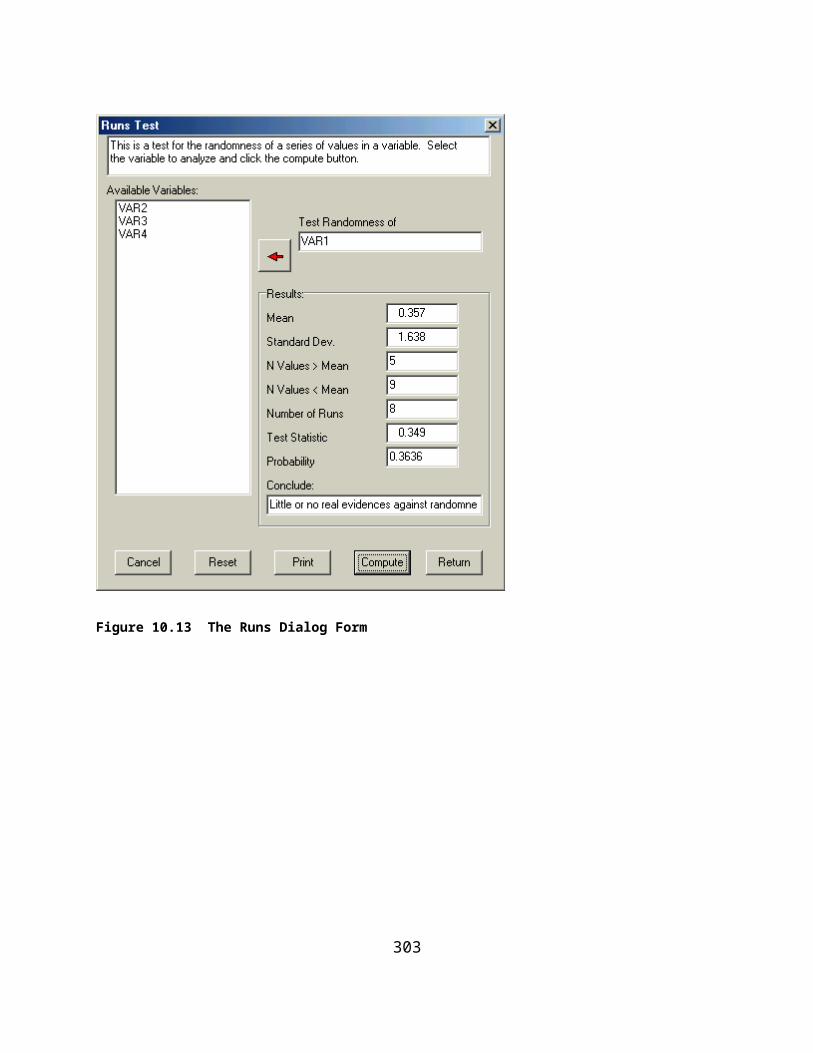
Figure 11.20 Level Means for Polytomous Item
For Item 2:
Observed Category FrequenciesItem Group Level Category Number 1 2 3 4 5 2 Ref. 1 56 46 47 48 51 2 Focal 1 37 38 49 35 48 2 Total 1 93 84 96 83 99
2 Ref. 2 2 0 0 0 0 2 Focal 2 1 0 0 0 0 2 Total 2 3 0 0 0 0
2 Ref. 3 12 8 1 0 0 2 Focal 3 9 11 1 0 0 2 Total 3 21 19 2 0 0
t-test values for Reference and Focus Means for each levelMean Reference = 2.968 SD = 23.046 N = 248Mean Focal = 3.092 SD = 22.466 N = 207Level 1 t = 0.058 with deg. freedom = 453Mean Reference = 2.000 SD = 2.000 N = 2Mean Focal = 1.000 SD = 1.000 N = 1Level 2 t = 0.000 with deg. freedom = 0Mean Reference = 1.476 SD = 4.262 N = 21Mean Focal = 1.619 SD = 5.094 N = 21Level 3 t = 0.096 with deg. freedom = 40Composite z statistic = 0.075. Prob. > |z| = 0.470Weighted Composite z statistic = 0.673. Prob. > |z| = 0.250Generalized Mantel-Haenszel = 1.017 with D.F. = 1 and Prob. > Chi-Sqr. = 0.313
Observed Category FrequenciesItem Group Level Category Number 1 2 3 4 5 3 Ref. 1 35 38 52 68 55
303

3 Focal 1 42 41 37 42 45 3 Total 1 77 79 89 110 100
3 Ref. 2 2 0 0 0 0 3 Focal 2 1 0 0 0 0 3 Total 2 3 0 0 0 0
3 Ref. 3 8 10 3 0 0 3 Focal 3 7 10 4 0 0 3 Total 3 15 20 7 0 0
t-test values for Reference and Focus Means for each levelMean Reference = 3.282 SD = 26.866 N = 248Mean Focal = 3.034 SD = 21.784 N = 207Level 1 t = -0.107 with deg. freedom = 453Mean Reference = 2.000 SD = 2.000 N = 2Mean Focal = 1.000 SD = 1.000 N = 1Level 2 t = 0.000 with deg. freedom = 0Mean Reference = 1.762 SD = 4.898 N = 21Mean Focal = 1.857 SD = 5.102 N = 21Level 3 t = 0.060 with deg. freedom = 40Composite z statistic = -0.023. Prob. > |z| = 0.509Weighted Composite z statistic = -1.026. Prob. > |z| = 0.848Generalized Mantel-Haenszel = 3.248 with D.F. = 1 and Prob. > ChiSqr. = 0.071
304

Generate Test Data
To help you become familiar with some of the measurement procedures, you can experiment by creating “artificial” item responses to a test. When you select the option to generate simulated test data, you complete the information in the following specification form. An example is shown. Before you begin, be sure you have closed any open file already in the data grid since the data that is generated will be placed in that grid.
Figure 11.21 The Item Generation Dialog
Shown below is a “snap-shot” of the generated test item responses. An additional row has been inserted for the first case which consists of all 1’s. It will serve as the “correct” response for scoring each of the item responses of the subsequent cases. You can save your generated file for future analyses or other work.
Figure 11.22 Generated Item Data in the Main Grid
Notice that in our example we specified the creation of test data that would have a reliability of 0.8 for 30 items administered to 100 students. If we analyze this data with our Classical Test Analysis procedure, we obtain the following output:
Alpha Reliability Estimate for Test = 0.8997 S.E. of Measurement = 2.406
305

Clearly, the test generated from our population specifications yielded a somewhat higher reliability than the 0.8 specified for the reliability. Have we learned something about sampling variability? If you request that the total be placed in the data grid when you use analyze the test, you can also use the descriptive statistics procedure to obtain the sample mean, etc. as shown below:
DISTRIBUTION PARAMETER ESTIMATES
TOTAL (N = 100) Sum = 1560.000Mean = 15.600 Variance = 55.838 Std.Dev. = 7.473Std.Error of Mean = 0.747Range = 29.000 Minimum = 1.000 Maximum = 30.000Skewness = -0.134 Std. Error of Skew = 0.241Kurtosis = -0.935 Std. Error Kurtosis = 0.478
The frequencies procedure can plot the total score distribution of our sample with the normal curve as a reference to obtain:
Figure 11.23 Plot of Generated Test Data
A test of normality of the total scores suggests a possibility that the obtained scores are not normally distributed as shown in the normality test form below:
306

Figure 11.24 Test of Normality for Generated Data
307

Spearman-Brown Reliability Prophecy
The Spearman-Brown "Prophecy" formula has been a corner-stone of many instructional text books in measurement theory. Based on "Classical True-Score" theory, it provides an estimate of what the reliability of a test of a different length would be based on the initial test's reliability estimate. It assumes the average difficulty and inter-item covariances of the extended (or trimmed) test are the same as the original test. If these assumptions are valid, it is a reasonable estimator. Shown below is the specification form which appears when you elect this Measurement option from the Analyses menu:
Figure 11.25 Spearman-Brown Prophecy Dialog
You can see that in an example, that when a test with an initial reliability of 0.8 is doubled (the multiplier k = 2) that the new test is expected to have a reliability of 0.89 approximately. The program may be useful for reducing a test (perhaps by randomly selecting items to delete) that requires too long to administer and has an initially high internal consistency reliability estimate. For example, assume a test of 200 items has a reliability of .95. What is the estimate if the test is reduced by one-half? If the new reliability of 0.9 is satisfactory, considerable time and money may be saved!
308
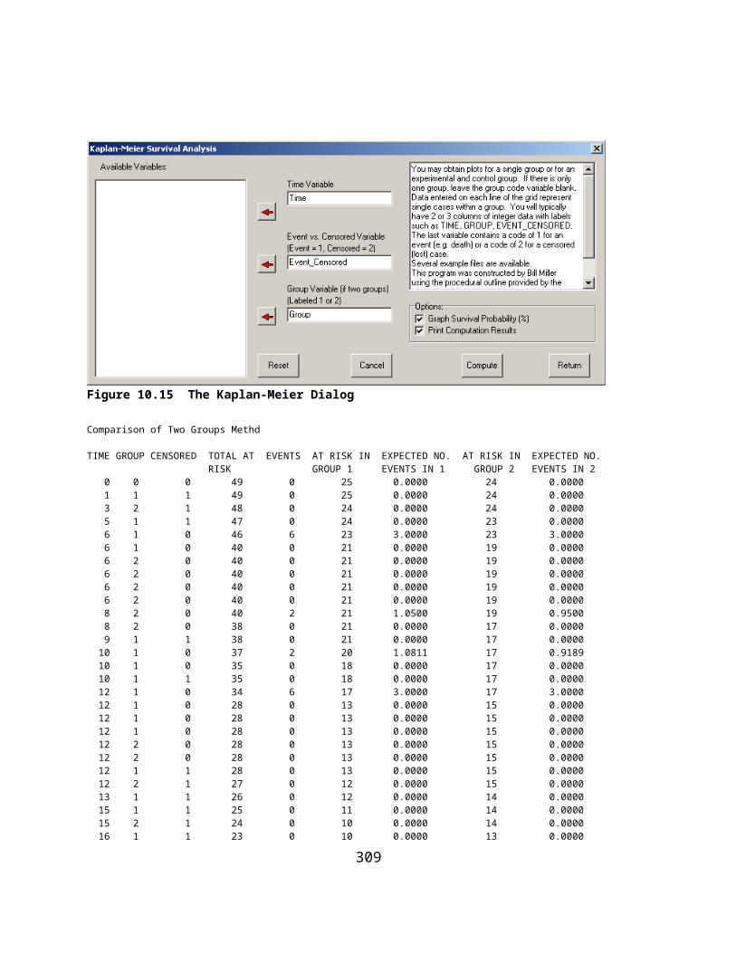
XII. Statistical Process Control
XBAR Chart
An Example
We will use the file labeled boltsize.txt to demonstrate the XBAR Chart procedure. Load the file and select the option Statistics / Statistical Process Control / Control Charts / XBAR Chart from the menu. The file contains two variables, lot number and bolt length. These values have been entered in the specification form which is shown below. Notice that the form also provides the option to enter and use a specific “target” value for the process as well as specification levels which may have been provided as guidelines for determining whether or not the process was in control for a given sample.
Figure 12.1 XBAR Chart Dialog
Pressing the Compute button results in the following:
X Bar Chart Results
Group Size Mean Std.Dev._____ ____ _________ __________ 1 5 19.88 0.37 2 5 19.90 0.29 3 5 20.16 0.27
309

4 5 20.08 0.29 5 5 19.88 0.49 6 5 19.90 0.39 7 5 20.02 0.47 8 5 19.98 0.43Grand Mean = 19.97, Std.Dev. = 0.359, Standard Error of Mean = 0.06Lower Control Limit = 19.805, Upper Control Limit = 20.145
310

Figure 12.2 XBAR Chart for Boltsize
If, in addition, we specify a target value of 20 for our bolt and upper and lower specification levels (tolerance) of 20.1 and 19.9, we would obtain the chart shown below:
311

Figure 12.3 XBAR Chart Plot with Target Specifications
In this chart we can see that the mean of the samples falls slightly below the specified target value and that samples 3 and 5 appear to have bolts outside the tolerance specifications.
Range Chart
As tools wear the products produced may begin to vary more and more widely around the values specified for them. The mean of a sample may still be close to the specified value but the range of values observed may increase. The result is that more and more parts produced may be under or over the specified value. Therefore quality assurance personnel examine not only the mean (XBAR chart) but also the range of values in their sample lots. Again, examine the boltsize.txt file with the option Statistics / Statistical Process Control / Control Charts / Range Chart. Shown below is the specification form and the results:
Figure 12.4 Range Chart Dialog
X Bar Chart Results
Group Size Mean Range Std.Dev._____ ____ _________ _______ ________ 1 5 19.88 0.90 0.37 2 5 19.90 0.70 0.29 3 5 20.16 0.60 0.27 4 5 20.08 0.70 0.29 5 5 19.88 1.20 0.49 6 5 19.90 0.90 0.39 7 5 20.02 1.10 0.47 8 5 19.98 1.00 0.43Grand Mean = 19.97, Std.Dev. = 0.359, Standard Error of Mean = 0.06Mean Range = 0.89Lower Control Limit = 0.000, Upper Control Limit = 1.876
312

Figure 12.5 Range Chart Plot
In the previous analysis using the XBAR chart procedure we found that the means of lots 3 and 6 were a meaningful distance from the target specification. In this chart we observed that lot 3 also had a larger range of values. The process appears out of control for lot 3 while for lot 6 it appears that the process was simply requiring adjustment toward the target value. In practice we would more likely see a pattern of increasing ranges as a machine becomes “loose” due to wear even though the averages may still be “on target”.
S Control Chart
The sample standard deviation, like the range, is also an indicator of how much values vary in a sample. While the range reflects the difference between largest and smallest values in a sample, the standard deviation reflects the square root of the average squared distance around the mean of the values. We desire to reduce this variability in our processes so as to produce products as similar to one another as is possible. The S control chart plot the standard deviations of our sample lots and allows us to see the impact of adjustments and improvements in our manufacturing processes.
Examine the boltsize.txt data with the S Control Chart. Shown below is the specification form for the analysis and the results obtained:
313

Figure 12.6 Sigma Chart Dialog
Group Size Mean Std.Dev._____ ____ _________ ________ 1 5 19.88 0.37 2 5 19.90 0.29 3 5 20.16 0.27 4 5 20.08 0.29 5 5 19.88 0.49 6 5 19.90 0.39 7 5 20.02 0.47 8 5 19.98 0.43Grand Mean = 19.97, Std.Dev. = 0.359, Standard Error of Mean = 0.06Mean Sigma = 0.37Lower Control Limit = 0.000, Upper Control Limit = 0.779
314

Figure 12.7 Sigma Chart Plot
The pattern of standard deviations is similar to that of the Range Chart.
315

CUSUM Chart
The specification form for the CUSUM chart is shown below for the data file labeled boltsize.txt. We have specified our desire to detect shifts of 0.02 in the process and are using the 0.05 and 0.20 probabilities for the two types of errors.
Figure 12.8 CUMSUM Chart Dialog
CUMSUM Chart Results
Group Size Mean Std.Dev. Cum.Dev. of mean from Target_____ ____ ________ ________ ___________ 1 5 19.88 0.37 -0.10 2 5 19.90 0.29 -0.18 3 5 20.16 0.27 0.00 4 5 20.08 0.29 0.10 5 5 19.88 0.49 0.00 6 5 19.90 0.39 -0.08 7 5 20.02 0.47 -0.04 8 5 19.98 0.43 -0.04Mean of group deviations = -0.005Mean of all observations = 19.975
316

Std. Dev. of Observations = 0.359Standard Error of Mean = 0.057Target Specification = 19.980Lower Control Limit = 19.805, Upper Control Limit = 20.145
Figure 12.9 CUMSUM Chart Plot
The results are NOT typical in that it appears that we have a process that is moving into control instead of out of control. Movement from lot 1 to 2 and from lot 3 to 4 indicate movement to out-of-control while the remaining values appear to be closer to in-control. If one checks the “Use the target value:” (of 20.0) the mask would indicate that lot 3 to 4 had moved to an out-of-control situation.
317

p Chart
To demonstrate the p Chart we will utilize a file labeled pchart.txt. Load the file and select the Analyses / Statistical Process Control / p Chart option. The specification form is shown below along with the results obtained after clicking the Compute Button:
Figure 12.10 p Control Chart Dialog
Target proportion = 0.0100Sample size for each observation = 1000Average proportion observed = 0.0116Defects p Control Chart Results
Sample No. Proportion__________ __________ 1 0.012 2 0.015 3 0.008 4 0.010 5 0.004 6 0.007 7 0.016 8 0.009 9 0.014 10 0.010 11 0.005
318
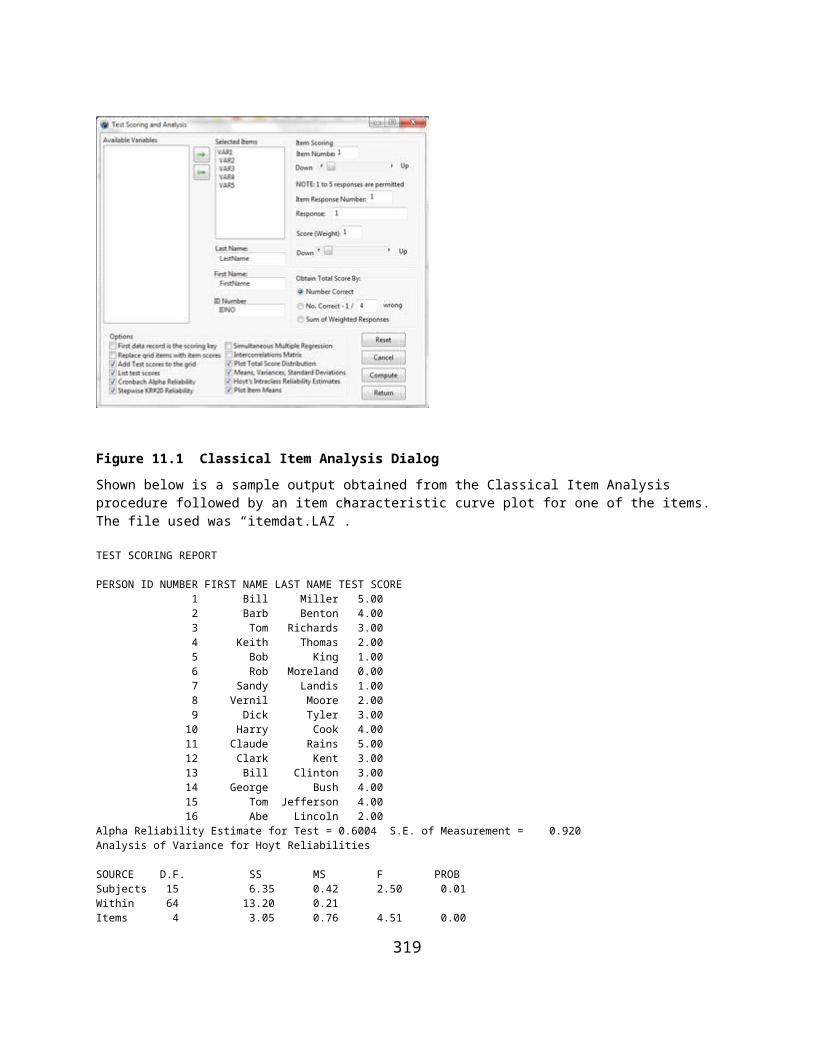
12 0.006 13 0.017 14 0.012 15 0.022 16 0.008 17 0.010 18 0.005 19 0.013 20 0.011 21 0.020 22 0.018 23 0.024 24 0.015 25 0.009 26 0.012 27 0.007 28 0.013 29 0.009 30 0.006Target proportion = 0.0100Sample size for each observation = 1000Average proportion observed = 0.0116
Figure 12.11 p Control Chart Plot
Several of the sample lots (N = 1000) had disproportionately high defect rates and would bear further examination of what may have been occurring in the process at those points.
319
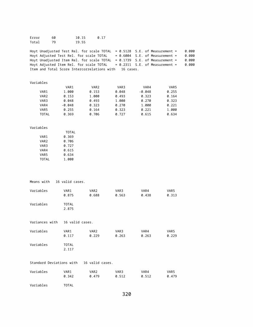
Defect (Non-conformity) c Chart
The previous section discusses the proportion of defects in samples (p Chart.) This section examines another defect process in which there is a count of defects in a sample lot. In this chart it is assumed that the occurrence of defects are independent, that is, the occurrence of a defect in one lot is unrelated to the occurrence in another lot. It is expected that the count of defects is quite small compared to the total number of parts potentially defective. For example, in the production of light bulbs, it is expected that in a sample of 1000 bulbs, only a few would be defective. The underlying assumed distribution model for the count chart is the Poisson distribution where the mean and variance of the counts are equal. Illustrated below is an example of processing a file labeled cChart.txt.
Figure 12.12 Defect c Chart Dialog
Defects c Control Chart Results
Sample Number of Noncomformities______ _______________ 1 7.00 2 6.00 3 6.00 4 3.00 5 22.00 6 8.00 7 6.00 8 1.00 9 0.00 10 5.00 11 14.00 12 3.00
320
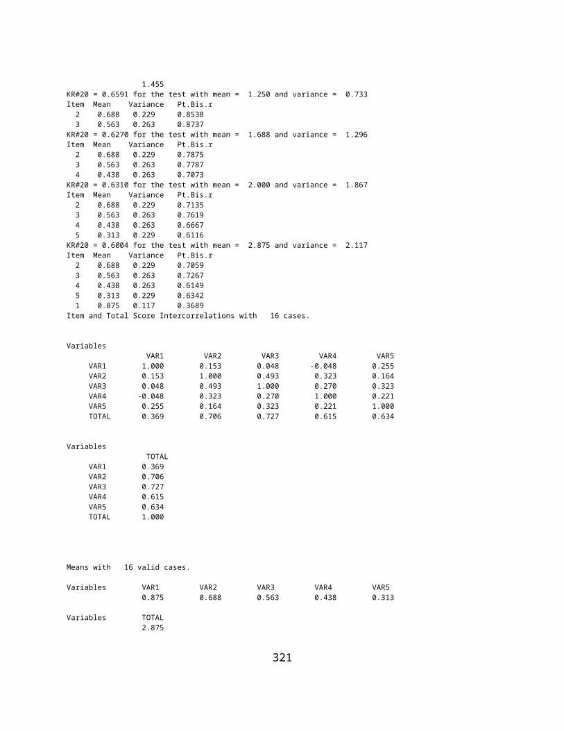
13 1.00 14 3.00 15 2.00 16 7.00 17 5.00 18 7.00 19 2.00 20 8.00 21 0.00 22 4.00 23 14.00 24 4.00 25 3.00Total Nonconformities = 141.00No. of samples = 25Poisson mean and variance = 5.640Lower Control Limit = -1.485, Upper Control Limit = 12.765
Figure 12.13 Defect Control Chart Plot
The count of defects for three of the 25 objects is greater than the upper control limit of three standard deviations.
321

Defects Per Unit u Chart
The specification form and results for the computation following the click of the Compute button are shown below:
Figure 12.14 Defects U Chart Dialog
Sample No Defects Defects Per Unit______ __________ ________________ 1 36.00 0.80 2 48.00 1.07 3 45.00 1.00 4 68.00 1.51 5 77.00 1.71 6 56.00 1.24 7 58.00 1.29 8 67.00 1.49 9 38.00 0.84 10 74.00 1.64 11 69.00 1.53 12 54.00 1.20 13 56.00 1.24 14 52.00 1.16 15 42.00 0.93 16 47.00 1.04 17 64.00 1.42 18 61.00 1.36 19 66.00 1.47 20 37.00 0.82
322

21 59.00 1.31 22 38.00 0.84 23 41.00 0.91 24 68.00 1.51 25 78.00 1.73Total Nonconformities = 1399.00No. of samples = 25Def. / unit mean = 1.244 and variance = 0.166Lower Control Limit = 0.745, Upper Control Limit = 1.742
Figure 12.15 Defect Control Chart Plot
In this example, the number of defects per unit are all within the upper and lower control limits.
323

XIII Linear Programming
The Linear Programming Procedure
To start the Linear Programming procedure, click on the Sub-Systems menu item and select the Linear Programming procedure. The following screen will appear:
Figure 13.1 Linear Programming Dialog
We have loaded a file named Metals.LPR by pressing the Load File button and selecting a file which we had already constructed to do the first problem given above. When you start a problem, you will typically enter the number of variables (X's) first. When you press the tab key to go to the next field or click on another area of the form, the grids which appear on the form will automatically reflect the correct number of columns for data entry. In the Metals problem we have 1 constraint of the 'Maximum' type, 1 constraint of the 'Minimum' type and 3 Equal constraints. When you have entered the number of each type of constraint the grids will automatically provide the correct number of rows for entry of the coefficients for those constraints. Next, we enter the 'Objective' or cost values. Notice that you do NOT enter a dollar sign, just the values for the variables - five in our example. Now we are ready to enter our constraints and the corresponding coefficients. Our first (maximum) constraint is set to 1000 to set an upper limit for the amount of metal to produce. This constraint applies to each of the variables and a value of 1.00 has been entered for the coefficients of this constraint. The one minimum constraint is entered next. In this case we have entered a value of 100 as the minimum amount to produce. Notice that the coefficients entered are ALL negative values of 1.0! You will be entering negative values for the Minimum and Equal constraints
324

coefficients. The constraint values themselves must all be zero or greater. We now enter the Equal constraint values and their coefficients from the second through the fourth equations. Again note that negative values are entered. Finally, we click on the Minimize button to indicate that we are minimizing the objective. We then press the Compute button to obtain the following results:
Linear Programming Results
X1 X5
z 544.8261 -0.1520 -0.7291 Y1 1100.0000 0.0000 0.0000 X3 47.8261 -0.7246 1.7391 Y2 0.0000 0.0000 0.0000 X4 41.7391 -0.0870 -2.3913 X2 10.4348 -0.1884 -0.3478
The first column provides the answers we sought. The cost of our new alloy will be minimal if we combine the alloys 2, 3 and 4 with the respective percentages of 10.4, 47.8 and 41.7. Alloys 1 and 5 are not used. The z value in the first column is our objective function value (544.8).
Next, we will examine the second problem in which the nutritionist desires to minimize costs for the optimal food mix. We will click the Reset button on the form to clear our previous problem and load a previously saved file labeled 'Nutrition.LPR'. The form appears below:
325

Figure 13.2 Example Specifications for a Linear Programming Problem
Again note that the minimum and equal constraint coefficients entered are negative values. When the compute button is pressed we obtain the following results:
Linear Programming Results
Y4 X2
z 0.4924 -0.0037 -0.1833 Y1 0.7000 0.0000 1.0000 Y2 33.2599 0.1666 3.7777 X1 0.8081 0.0122 -0.7222 Y3 0.7081 0.0122 -0.7222 X3 0.5000 0.0000 0.0000
In this solution we will be using .81 parts of Food A and .5 parts of Food C. Food B is not used.
326

The Linear Programming procedure of this program is one adapted from the Simplex program in the Numerical Recipes book listed in the bibliography (#56). The form design is one adapted from the Linear Programming program by Ane Visser of the AgriVisser consulting firm.
327

XIV USING MATMAN
Purpose of MatMan
MatMan was written to provide a platform for performing common matrix and vector operations. It is designed to be helpful for the student learning matrix algebra and statistics as well as the researcher needing a tool for matrix manipulation. If you are already a user of the OpenStat program, you can import files that you have saved with OpenStat into a grid of MatMan.
Using MatMan
When you first start the MatMan program, you will see the main program form below. This form displays four "grids" in which matrices, row or column vectors or scalars (single values) may be entered and saved. If a grid of data has already been saved, it can be retrieved into any one of the four grids. Once you have entered data into a grid, a number of operations can be performed depending on the type of data entered (matrix, vector or scalar.) Before performing an operation, you select the grid of data to analyze by clicking on the grid with the left mouse button. If the data in the selected grid is a matrix (file extension of .MAT) you can select any one of the matrix operations by clicking on the Matrix Operations "drop-down" menu at the top of the form. If the data is a row or column vector, select an operation option from the Vector Operations menu. If the data is a single value, select an operation from the Scalar Operations menu.
Figure 14.1 The MatMan Dialog
328

Using the Combination Boxes
In the upper right portion of the MatMan main form, there are four "Combo Boxes". These boxes each contain a drop-down list of file names. The top box labeled "Matrix" contains the list of files containing matrices that have been created in the current disk directory and end with an extension of .MAT. The next two combo boxes contain similar lists of column or row vectors that have been created and are in the current disk directory. The last contains name of scalar files that have been saved in the current directory. These combo boxes provide documentation as to the names of current files already in use. In addition, they provide a "short-cut" method of opening a file and loading it into a selected grid.
Files Loaded at the Start of MatMan
Five types of files are loaded when you first start the execution of the MatMan program. The program will search for files in the current directory that have file extensions of .MAT, .CVE, .RVE, .SCA and .OPT. The first four types of files are simply identified and their names placed into the corresponding combination boxes of matrices, column vectors, row vectors and scalars. The last, options, is a file which contains only two integers: a 1 if the script should NOT contain File Open operations when it is generated or a 0 and a 1 if the script should NOT contain File Save operations when a script is generated or a 0. Since File Open and File Save operations are not actually executed when a script or script line is executed, they are in a script only for documentation purposes and may be left out.
Clicking the Matrix List Items
A list of Matrix files in the current directory will exist in the Matrix "Drop-Down" combination box when the MatMan program is first started. By clicking on one of these file names, you can directly load the referenced file into a grid of your selection.
Clicking the Vector List Items
A list of column and row vector files in the current directory will exist in the corresponding column vector or row vector "Drop-Down" combination boxes when the MatMan program is first started. By clicking a file name in one of these boxes, you can directly load the referenced file into a grid of your selection.
Clicking the Scalar List Items
When you click on the down arrow of the Scalar "drop-down" combination box, a list of file names appear which have been previously loaded by identifying all scalar files in the current directory. Also listed are any new scalar files that you have created during a session with MatMan. If you move your mouse cursor down to a file name and click on it, the file by that name will be loaded into the currently selected grid or a grid of your choice.
The Grids
The heart of all operations you perform involve values entered into the cells of a grid. These values may represent values in a matrix, a column vector, a row vector or a scalar. Each grid is like a spreadsheet. Typically, you select the first row and column cell by clicking on that cell with the left mouse key when the mouse cursor is
329

positioned over that cell. To select a particular grid, click the left mouse button when the mouse cursor is positioned over any cell of that grid. You will then see that the grid number currently selected is displayed in a small text box in the upper left side of the form (directly below the menus.)
Operations and Operands
At the bottom of the form (under the grids) are four "text" boxes labeled Operation, Operand1, Operand2 and Operand3. Each time you perform an operation by use of one of the menu options, you will see an abbreviation of that operation in the Operation box. Typically there will be at least one or two operands related to that operation. The first operand is typically the name of the data file occupying the current grid and the second operand the name of the file containing the results of the operation. Some operations involve two grids, for example, adding two matrices. In these cases, the name of the two grid files involved will be in operands1 and operands2 boxes while the third operand box will contain the file for the results.
You will also notice that each operation or operand is prefixed by a number followed by a dash. In the case of the operation, this indicates the grid number from which the operation was begun. The numbers which prefix the operand labels indicate the grid in which the corresponding files were loaded or saved. The operation and operands are separated by a colon (:). When you execute a script line by double clicking an operation in the script list, the files are typically loaded into corresponding grid numbers and the operation performed.
Menus
The operations which may be performed on or with matrices, vectors and scalars are all listed as options under major menu headings shown across the top of the main form. For example, the File menu, when selected, provides a number of options for loading a grid with file data, saving a file of data from a grid, etc. Click on a menu heading and explore the options available before you begin to use MatMan. In nearly all cases, when you select a menu option you will be prompted to enter additional information. If you select an option by mistake you can normally cancel the operation.
Combo Boxes
Your main MatMan form contains what are known as "Drop-Down" combination boxes located on the right side of the form. There are four such boxes: The "Matrix" box, the "Column Vectors" box, the "Row Vectors" box and the "Scalars" box. At the right of each box is an arrow which, when clicked, results in a list of items "dropped-down" into view. Each item in a box represents the name of a matrix, vector or scalar file in the current directory or which has been created by one of the possible menu operations. By clicking on one of these items, you initiate the loading of the file containing the data for that matrix, vector or scalar. You will find this is a convenient alternative to use of the File menu for opening files which you have been working with. Incidentally, should you wish to delete an existing file, you may do so by selecting the "edit" option under the Script menu. The script editor lists all files in a directory and lets you delete a file by simply double-clicking the file name!
The Operations Script
Located on the right side of the main form is a rectangle which may contain operations and operands performed in using MatMan. This list of operations and their corresponding operands is known collectively as a "Script". If you were to perform a group of operations, for example, to complete a multiple regression analysis, you may want to save the script for reference or repeated analysis of another set of data. You can also edit the scripts
330

that are created to remove operations you did not intend, change the file names referenced, etc. Scripts may also be printed.
Getting Help on a Topic
You obtain help on a topic by first selecting a menu item, grid or other area of the main form by placing the mouse over the item for which you want information. Once the area of interest is selected, press the F1 key on your keyboard. If a topic exists in the help file, it will be displayed. You can press the F1 key at any point to bring up the help file. A book is displayed which may be opened by double clicking it. You may also search for a topic using the help file index of keywords.
Scripts
Each time an operation is performed on grid data, an entry is made in a "Script" list shown in the right-hand portion of the form. The operation may have one to three "operands" listed with it. For example, the operation of finding the eigenvalues and eigenvectors of a matrix will have an operation of SVDInverse followed by the name of the matrix being inverted, the name of the eigenvalues matrix and the name of the eigenvectors matrix. Each part of the script entry is preceded by a grid number followed by a hyphen (-). A colon separates the parts of the entry (:). Once a series of operations have been performed the script that is produced can be saved. Saved scripts can be loaded at a later time and re-executed as a group or each entry executed one at a time. Scripts can also be edited and re-saved. Shown below is an example script for obtaining multiple regression coefficients.
CURRENT SCRIPT LISTING:
FileOpen:1-newcansas1-ColAugment:newcansas:1-X1-FileSave:1-X.MAT1-MatTranspose:1-X:2-XT2-FileSave:2-XT.MAT2-PreMatxPostMat:2-XT:1-X:3-XTX3-FileSave:3-XTX.MAT3-SVDInverse:3-XTX.MAT:1-XTXINV1-FileSave:1-XTXINV.MATFileOpen:1-XT.MATFileOpen:2-Y.CVE1-PreMatxPostVec:1-XT.MAT:2-Y.CVE:3-XTY3-FileSave:3-XTY.CVEFileOpen:1-XTXINV.MAT1-PreMatxPostVec:1-XTXINV.MAT:3-XTY:4-BETAS4-FileSave:4-Bweights.CVE
To print a script which appears in the Script List, move your mouse to the Script menu and click on the Print option. The list will be printed on the Output Form. At the bottom of the form is a print button that you can click with the mouse to get a hard-copy output.
331

Clear Script List
To clear an existing script from the script list, move the mouse to the Script menu and click the Clear option. Note: you may want to save the script before clearing it if it is a script you want to reference at a later time.
Edit the Script
Occasionally you may want to edit a script you have created or loaded. For example, you may see a number of Load File or Save File operations in a script. Since these are entered only for documentation and cannot actually be executed by clicking on them, they can be removed from the script. The result is a more compact and succinct script of operations performed. You may also want to change the name of files accessed for some operations or the name of files saved following an operation so that the same operations may be performed on a new set of data. To begin editing a script, move the mouse cursor to the Script menu and click on the Edit option. A new form appears which provides options for the editing. The list of operations appears on the left side of the form and an Options box appears in the upper right portion of the form. To edit a given script operation, click on the item to be edited and then click one of the option buttons. One option is to simply delete the item. Another is to edit (modify) the item. When that option is selected, the item is copied into an "Edit Box" which behaves like a miniature word processor. You can click on the text of an operation at any point in the edit box, delete characters following the cursor with the delete key, use the backspace key to remove characters in front of the cursor, and enter characters at the cursor. When editing is completed, press the return key to place the edited operation back into the script list from which it came.
Also on the Edit Form is a "Directory Box" and a "Files Box". Shown in the directory box is the current directory you are in. The files list box shows the current files in that directory. You can delete a file from any directory by simply double-clicking the name of the file in the file list. A box will pop up to verify that you want to delete the selected file. Click OK to delete the file or click Cancel if you do not want to delete the file. CAUTION! Be careful NOT to delete an important file like MATMAN.EXE, MATMAN.HLP or other system files (files with extensions of .exe, .dll, .hlp, .inf, etc.! Files which ARE safe to delete are those you have created with MatMan. These all end with an extension of .MAT, .CVE, .RVE ,.SCA or .SCR .
Load a Script
If you have saved a script of matrix operations, you can re-load the script for execution of the entire script of operations or execution of individual script items. To load a previously saved script, move the mouse to the Script menu and click on the Load option. Alternatively, you can go to the File menu and click on the Load Script option. Operation scripts are saved in a file as text which can also be read and edited with any word processing program capable of reading ASCII text files. For examples of scripts that perform statistical operations in matrix notation, see the help book entitled Script Examples.
Save a Script
Nearly every operation selected from one of the menus creates an entry into the script list. This script provides documentation of the steps performed in carrying out a sequence of matrix, vector or scalar operations. If you save the script in a file with a meaningful name related to the operations performed, that script may be "re-used" at a later time.
Executing a Script
332

You may quickly repeat the execution of a single operation previously performed and captured in the script. Simply click on the script item with the left mouse button when the cursor is positioned over the item to execute. Notice that you will be prompted for the name of the file or files to be opened and loaded for that operation. You can, of course, choose a different file name than the one or ones previously used in the script item. If you wish, you can also re-execute the entire script of operations. Move your mouse cursor to the Script menu and click on the Execute option. Each operation will be executed in sequence with prompts for file names appearing before execution each operation. Note: you will want to manually save the resulting file or files with appropriate names.
Script Options
File Open and File Save operations may or may not appear in a script list depending on options you have selected and saved. Since these two operations are not executed when a script is re-executed, it is not necessary that they be saved in a script (other than for documentation of the steps performed.) You can choose whether or not to have these operations appear in the script as you perform matrix, vector or scalar operations. Move your mouse cursor to the Script menu and click on the Options option. A pop-up form will appear on which you can elect to save or not save the File Open and File Save operations. The default (unchecked) option is to save these operations in a script. Clicking on an option tells the program to NOT write the operation to the script. Return to the MatMan main form by clicking the Return or Cancel button.
Files
When MatMan is first started it searches the current directory of your disk for any matrices, column vectors, row vectors or scalars which have previously been saved. The file names of each matrix, vector or scalar are entered into a drop-down list box corresponding to the type of data. These list boxes are located in the upper right portion of the main form. By first selecting one of the four grids with a click of the left mouse button and then clicking on one of the file names in a drop-down list, you can automatically load the file in the selected grid. Each time you save a grid of data with a new name, that file name is also added to the appropriate file list (Matrix, Column Vector, Row Vector or Scalar.)
At the top of the main form is a menu item labeled "Files". By clicking on the Files menu you will see a list of file options as shown in the picture below. In addition to saving or opening a file for a grid, you can also import an OpenStat .txt file, import a file with tab-separated values, import a file with comma separated values or import a file with spaces separating the values. All files saved with MatMan are ASCII text files and can be read (and edited if necessary) with any word processor program capable of reading ASCII files (for example the Windows Notepad program.)
333

Figure 14.2 Using the MatMan Files Menu
Keyboard Input
You can input data into a grid directly from the keyboard to create a file. The file may be a matrix, row vector, column vector or a scalar. Simply click on one of the four grids to receive your keystrokes. Note that the selected grid number will be displayed in a small box above and to the left of the grids. Next, click on the Files menu and move your cursor down to the Keyboard entry option. You will see that this option is expanded for you to indicate the type of data to be entered. Click on the type of data to be entered from the keyboard. If you selected a matrix, you will be prompted for the number of rows and columns of the matrix. For a vector, you will be prompted for the type (column or row) and the number of elements. Once the type of data to be entered and the number of elements are known, the program will "move" to the pre-selected grid and be waiting for your data entry. Click on the first cell (Row 1 and Column 1) and type your (first) value. Press the tab key to move to the next element in a row or, if at the end of a row, the first element in the next row. When you have entered the last value, instead of pressing the tab key, press the return key. You will be prompted to save the data. Of course, you can also go to the Files menu and click on the Save option. This second method is particularly useful if you are entering a very large data matrix and wish to complete it in several sessions.
File Open
If you have previously saved a matrix, vector or scalar file while executing the MatMan program, it will have been saved in the current directory (where the MatMan program resides.) MatMan saves data of a matrix type with a file extension of .MAT. Column vectors are saved with an extension of .CVE and row vectors saved with an extension of .RVE. Scalars have an extension of .SCA. When you click the File Open option in the File menu, a dialogue box appears. In the lower part of the box is an indication of the type of file. Click on this drop-down box to see the various extensions and click on the one appropriate to the type of file to be loaded. Once you have done
334

that, the files listed in the files box will be only the files with that extension. Since the names of all matrix, vector and scalar files in the current directory are also loaded into the drop-down boxes in the upper right portion of the MatMan main form, you can also load a file by clicking on the name of the file in one of these boxes. Typically, you will be prompted for the grid number of the grid in which to load the file. The grid number is usually the one you have previously selected by clicking on a cell in one of the four grids.
File Save
Once you have entered data into a grid or have completed an operation producing a new output grid, you may save it by clicking on the save option of the File menu. Files are automatically saved with an extension which describes the type of file being saved, that is, with a .MAT, .CVE, .RVE or .SCA extension. Files are saved in the current directory unless you change to a different directory from the save dialogue box which appears when you are saving a file. It is recommended that you save files in the same directory (current directory) in which the MatMan program resides. The reason for doing this is that MatMan automatically loads the names of your files in the drop-down boxes for matrices, column vectors, row vectors and scalars.
Import a File
In addition to opening an existing MatMan file that has an extension of .MAT, .CVE, .RVE or .SCA, you may also import a file created by other programs. Many word processing and spread -sheet programs allow you to save a file with the data separated by tabs, commas or spaces. You can import any one of these types of files. Since the first row of data items may be the names of variables, you will be asked whether or not the first line of data contains variable labels.You may also import files that you have saved with the OpenStat2 program. These files have an extension of .TXT or .txt when saved by the OpenStat2 program. While they are ASCII type text files, they contain a lot of information such as variable labels, long labels, format of data, etc. MatMan simply loads the variable labels, replacing the column labels currently in a grid and then loads numeric values into the grid cells of the grid you have selected to receive the data.
Export a File
You may wish to save your data in a form which can be imported into another program such as OpenStat, Excel, MicroSoft Word, WordPerfect, etc. Many programs permit you to import data where the data elements have been separated by a tab, comma or space character. The tab character format is particulary attractive because it creates an ASCII (American Standard Code for Information Interchange) file with clearly delineated spacing among values and which may be viewed by most word processing programs.
Open a Script File
Once you have performed a number of operations on your data you will notice that each operation has been "summarized" in a list of script items located in the script list on the right side of the MatMan form. This list of operations may be saved for later reference or re-execution in a file labeled appropriate to the series of operations. To re-open a script file, go to the File Menu and select the Open a Script File option. A dialogue box will appear. Select the type of file with an extension of .SCR and you will see the previously saved script files listed. Click on
335

the one to load and press the OK button on the dialogue form. Note that if a script is already in the script list box, the new file will be added to the existing one. You may want to clear the script list box before loading a previously saved script. Clear the script list box by selecting the Clear option under the Script Operations menu.
Save the Script
Once a series of operations have been performed on your data, the operations performed will be listed in the Script box located to the right of the MatMan form. The series of operations may represent the completion of a data analysis such as multiple regression, factor analysis, etc. You may save this list of operations for future reference or re-execution. To save a script, select the Save Script option from the File Menu. A dialogue box will appear in which you enter the name of the file. Be sure that the type of file is selected as a .SCR file (types are selected in the drop-down box of the dialogue form.) A file extension of .SCR is automatically appended to the name you have entered. Click on the OK button to complete the saving of the script file.
Reset All
Occasionally you may want to clear all grids of data and clear all drop-down boxes of currently listed matrix, vector and scalar files. To do so, click the Clear All option under the Files Menu. Note that the script list box is NOT cleared by this operation. To clear a script, select the Clear operation under the Script Operations menu.
Entering Grid Data
Grids are used to enter matrices, vectors or scalars. Select a grid for data by moving the mouse cursor to the one of the grids and click the left mouse button. Move your mouse to the Files menu at the top of the form and click it with the left mouse button. Bring your mouse down to the Keyboard Input option. For entry of a matrix of values, click on the Matrix option. You will then be asked to verify the grid for entry. Press return if the grid number shown is correct or enter a new grid number and press return. You will then be asked to enter the name of your matrix (or vector or scalar.) Enter a descriptive name but keep it fairly short. A default extension of .MAT will automatically be appended to matrix files, a .CVE will be appended to column vectors, a .RVE appended to row vectors and a .SCA appended to a scalar. You will then be prompted for the number of rows and the number of columns for your data. Next, click on the first available cell labeled Col.1 and Row 1. Type the numeric value for the first number of your data. Press the tab key to move to the next column in a row (if you have more than one column) and enter the next value. Each time you press the tab key you will be ready to enter a value in the next cell of the grid. You can, of course, click on a particular cell to edit the value already entered or enter a new value. When you have entered the last data value, press the Enter key. A "Save" dialog box will appear with the name you previously chose. You can keep this name or enter a new name and click the OK button. If you later wish to edit values, load the saved file, make the changes desired and click on the Save option of the Files menu.
When a file is saved, an entry is made in the Script list indicating the action taken. If the file name is not already listed in one of the drop-down boxes (e.g. the matrix drop-down box), it will be added to that list.
Clearing a Grid
Individual grids are quickly reset to a blank grid with four rows and four columns by simply moving the mouse cursor over a cell of the grid and clicking the RIGHT mouse button. CAUTION! Be sure the data already in the grid has been saved if you do not want to lose it!
336

Inserting a Column
There may be occasions where you need to add another variable or column of data to an existing matrix of data. You may insert a new blank column in a grid by selecting the Insert Column operation under the Matrix Operations menu. First, click on an existing column in the matrix prior to or following the cell where you want the new column inserted. Click on the Insert Column option. You will be prompted to indicate whether the new column is to precede or follow the currently selected column. Indicate your choice and click the Return button.
Inserting a Row
There may be occasions where you need to add another subject or row of data to an existing matrix of data. You may insert a new blank row in a grid by selecting the Insert Row operation under the Matrix Operations menu. First, click on an existing row in the matrix prior to or following the cell where you want the new row inserted. Click on the Insert Row option. You will be prompted to indicate whether the new row is to precede or follow the number of the selected row. Indicate your choice and click the Return button.
Deleting a Column
To delete a column of data in an existing data matrix, click on the grid column to be deleted and click on the Delete Column option under the Matrix Operations menu. You will be prompted for the name of the new matrix to save. Enter the new matrix name (or use the current one if the previous one does not need to be saved) and click the OK button.
Deleting a Row
To delete a row of data in an existing data matrix, click on the grid row to be deleted and click on the Delete Row option under the Matrix Operations menu. You will be prompted for the name of the new matrix to save. Enter the new matrix name (or use the current one if the previous one does not need to be saved) and click the OK button.
Using the Tab Key
You can navigate through the cells of a grid by simply pressing the tab key. Of course, you may also click the mouse button on any cell to select that cell for data entry or editing. If you are at the end of a row of data and you press the tab key, you are moved to the first cell of the next row (if it exists.) To save a file press the Return key when located in the last row and column cell.
Using the Enter Key
If you press the Return key after entering the last data element in a matrix, vector or scalar, you will automatically be prompted to save the file. A "save" dialogue box will appear in which you enter the name of the file to save your data. Be sure the type of file to be saved is selected before you click the OK button.
337
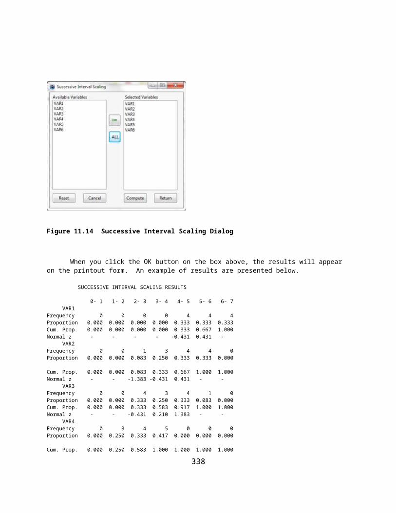
Editing a Cell Value
Errors in data entry DO occur (after all, we are human aren't we?) You can edit a data element by simply clicking on the cell to be edited. If you double click the cell, it will be highlighted in blue at which time you can press the delete key to remove the cell value or enter a new value. If you simply wish to edit an existing value, click the cell so that it is NOT highlighted and move the mouse cursor to the position in the value at which you want to start editing. You can enter additional characters, press the backspace key to remove a character in front of the cursor or press the delete key to remove a character following the cursor. Press the tab key to move to the next cell or press the Return key to obtain the save dialogue box for saving your corrections.
Loading a File
Previously saved matrices, vectors or scalars are easily loaded into any one of the four grids. First select a grid to receive the data by clicking on one of the cells of the target grid. Next, click on the Open File option under the Files Menu. An "open" dialogue will appear which lists the files in your directory. The dialogue has a drop-down list of possible file types. Select the type for the file to be loaded. Only files of the selected type will then be listed. Click on the name of the file to load and click the OK button to load the file data.
Matrix Operations
Once a matrix of data has been entered into a grid you can elect to perform a number of matrix operations. The figure below illustrates the options under the Matrix Operations menu. Operations include:
Row AugmentColumn AugmentDelete a RowDelete a ColumnExtract Col. Vector from MatrixSVD InverseTridiagonalizeUpper-Lower DecompositionDiagonal to VectorDeterminantNormalize RowsNormalize ColumnsPremultiply by : Row Vector; Matrix;ScalerPostmultiply by : Column Vector; MatrixEigenvalues and VectorsTransposeTraceMatrix A + Matrix BMatrix A - Matrix BPrint
Printing
338

You may elect to print a matrix, vector, scalar or file. When you do, the output is placed on an "Output" form. At the bottom of this form is a button labeled "Print" which, if clicked, will send the contents of the output form to the printer. Before printing this form, you may type in additional information, edit lines, cut and paste lines and in general edit the output to your liking. Edit operations are provided as icons at the top of the form. Note that you can also save the output to a disk file, load another output file and, in general, use the output form as a word processor.
Row Augment
You may add a row of 1's to a matrix with this operation. When the transpose of such an augmented matrix is multiplied times this matrix, a cell will be created in the resulting matrix, which contains the number of columns in the augmented matrix.
Column Augmentation
You may add a column of 1's to a matrix with this operation. When the transpose of such an augmented matrix is multiplied times this matrix, a cell will be created in the resulting matrix, which contains the number of rows in the augmented matrix. The procedure for completing a multiple regression analysis often involves column augmentation of a data matrix containing a row for each object (e.g. person) and column cells containing independent variable values. The column of 1's created from the Column Augmentation process ends up providing the intercept (regression constant) for the analysis.
Extract Col. Vector from Matrix
In many statistics programs the data matrix you begin with contains columns of data representing independent variables and one or more columns representing dependent variables. For example, in multiple regression analysis, one column of data represents the dependent variable (variable to be predicted) while one or more columns represent independent variables (predictor variables.) To analyze this data with the MatMan program, one would extract the dependent variable and save it as a column vector for subsequent operations (see the sample multiple regression script.) To extract a column vector from a matrix you first load the matrix into one of the four grids, click on a cell in the column to be extracted and then click on the Extract Col. Vector option under the Matrix Operations menu.
SVDInverse
A commonly used matrix operation is the process of finding the inverse (reciprocal) of a symmetric matrix. A variety of methods exist for obtaining the inverse (if one exists.) A common problem with some inverse methods is that they will not provide a solution if one of the variables is dependent (or some combination of) on other variables (rows or columns) of the matrix. One advantage of the "Singular Value Decomposition" method is that it typically provides a solution even when one or more dependent variables exist in the matrix. The offending variable(s) are essentially replaced by zeroes in the row and column of the dependent variable. The resulting inverse will NOT be the desired inverse.
To obtain the SVD inverse of a matrix, load the matrix into a grid and click on the SVDInverse option from the Matrix Operations menu. The results will be displayed in grid 1 of the main form. In addition, grids 2 through 4 will contain additional information which may be helpful in the analysis. Figures 1 and 2 below illustrate the results
339

of inverting a 4 by 4 matrix, the last column of which contains values that are the sum of the first three column cells in each row (a dependent variable.)
When you obtain the inverse of a matrix, you may want to verify that the resulting inverse is, in fact, the reciprocal of the original matrix. You can do this by multiplying the original matrix times the inverse. The result should be a matrix with 1's in the diagonal and 0's elsewhere (the identity matrix.) Figure 3 demonstrates that the inverse was NOT correct, that is, did not produce an identity matrix when multiplied times the original matrix.
Figure 1. DepMat.MAT From Grid Number 1
Columns Col.1 Col.2 Col.3 Col.4 Rows 1 5.000 11.000 2.000 18.000 2 11.000 2.000 4.000 17.000 3 2.000 4.000 1.000 7.000 4 18.000 17.000 7.000 1.000
Figure 2. DepMatInv.MAT From Grid Number 1
Columns Col.1 Col.2 Col.3 Col.4 Rows 1 0.584 0.106 -1.764 0.024 2 0.106 -0.068 -0.111 0.024 3 -1.764 -0.111 4.802 0.024 4 0.024 0.024 0.024 -0.024
Figure 3. DepMatxDepMatInv.MAT From Grid Number 3
Columns Col.1 Col.2 Col.3 Col.4 Rows 1 1.000 0.000 0.000 0.000 2 0.000 1.000 0.000 0.000 3 0.000 0.000 1.000 0.000 4 1.000 1.000 1.000 0.000
NOTE! This is NOT an Identity matrix.
340

Tridiagonalize
In obtaining the roots and vectors of a matrix, one step in the process is frequently to reduce a symetric matrix to a tri-diagonal form. The resulting matrix is then solved more readily for the eigenvalues and eigenvectors of the original matrix. To reduce a matrix to its tridiagonal form, load the original matrix in one of the grids and click on the Tridiagonalize option under the Matrix Operations menu.
Upper-Lower Decomposition
A matrix may be decomposed into two matrices: a lower matrix (one with zeroes above the diagonal) and an upper matrix (one with zeroes below the diagonal matrix.) This process is sometimes used in obtaining the inverse of a matrix. The matrix is first decomposed into lower and upper parts and the columns of the inverse solved one at a time using a routine that solves the linear equation A X = B where A is the upper/lower decomposition matrix, B are known result values of the equation and X is solved by the routine. To obtain the LU decomposition, enter or load a matrix into a grid and select the Upper-Lower Decomposition option from the Matrix Operations menu.
Diagonal to Vector
In some matrix algebra problems it is necessary to perform operations on a vector extracted from the diagonal of a matrix. The Diagonal to Vector operation extracts the the diagonal elements of a matrix and creates a new column vector with those values. Enter or load a matrix into a grid and click on the Diagonal to Vector option under the Matrix Operations menu to perform this operation.
Determinant
The determinant of a matrix is a single value characterizing the matrix values. A singular matrix (one for which the inverse does not exist) will have a determinant of zero. Some ill-conditioned matrices will have a determinant close to zero. To obtain the determinant of a matrix, load or enter a matrix into a grid and select the Determinant option from among the Matrix Operations options. Shown below is the determinant of a singular matrix (row/column 4 dependent on columns 1 through 3.)
Columns Col.1 Col.2 Col.3 Col.4 Rows 1 5.000 11.000 2.000 18.000 2 11.000 2.000 4.000 17.000 3 2.000 4.000 1.000 7.000 4 18.000 17.000 7.000 42.000
341

Columns Col 1 Rows
1 0.000
Normalize Rows or Columns
In matrix algebra the columns or rows of a matrix often represent vectors in a multi-dimension space. To make the results more interpretable, the vectors are frequently scaled so that the vector length is 1.0 in this "hyper-space" of k-dimensions. This scaling is common for statistical procedures such as Factor Analysis, Principal Component Analysis, Discriminant Analysis, Multivariate Analysis of Variance, etc. To normalize the row (or column) vectors of a matrix such as eigenvalues, load the matrix into a grid and select the Normalize Rows (or Normalize Columns) option from the Matrix Operations menu.
Pre-Multiply by:
A matrix may be multiplied by a row vector, another matrix or a single value (scalar.) When a row vector with N columns is multiplied times a matrix with N rows, the result is a row vector of N elements. When a matrix of N rows and M columns is multiplied times a matrix with M rows and Q columns, the result is a matrix of N rows and Q columns. Multiplying a matrix by a scalar results in each element of the matrix being multiplied by the value of the scalar.
To perform the pre-multiplication operation, first load two grids with the values of a matrix and a vector, matrix or scaler. Click on a cell of the grid containing the matrix to insure that the matrix grid is selected. Next, select the Pre-Multipy by: option and then the type of value for the pre-multiplier in the sub-options of the Matrix Operations menu. A dialog box will open asking you to enter the grid number of the matrix to be multiplied. The default value is the selected matrix grid. When you press the OK button another dialog box will prompt you for the grid number containing the row vector, matrix or scalar to be multiplied times the matrix. Enter the grid number for the pre-multiplier and press return. Finally, you will be prompted to enter the grid number where the results are to be displayed. Enter a number different than the first two grid numbers entered. You will then be prompted for the name of the file for saving the results.
Post-Multiply by:
A matrix may be multiplied times a column vector or another matrix. When a matrix with N rows and Q columns is multiplied times a column vector with Q rows, the result is a column vector of N elements. When a matrix of N rows and M columns is multiplied times a matrix with M rows and Q columns, the result is a matrix of N rows and Q columns.
To perform the post-multiplication operation, first load two grids with the values of a matrix and a vector or matrix. Click on a cell of the grid containing the matrix to insure that the matrix grid is selected. Next, select the Post-Multiply by: option and then the type of value for the post-multiplier in the sub-options of the Matrix Operations menu. A dialog box will open asking you to enter the grid number of the matrix multiplier. The default value is the selected matrix grid. When you press the OK button another dialog box will prompt you for the grid number containing the column vector or matrix. Enter the grid number for the post-multiplier and press return. Finally, you will be prompted to enter the grid number where the results are to be displayed. Enter a number different than the first two grid numbers entered. You will then be prompted for the name of the file for saving the results.
342

Eigenvalues and Vectors
Eigenvalues represent the k roots of a polynomial constructed from k equations. The equations are represented by values in the rows of a matrix. A typical equation written in matrix notation might be:
Y = B X
where X is a matrix of known "independent" values, Y is a column vector of "dependent" values and B is a column vector of coefficients which satisfies specified properties for the solution. An example is given when we solve for "least-squares" regression coefficients in a multiple regression analysis. In this case, the X matrix contains cross-products of k independent variable values for N cases, Y contains known values obtained as the product of the transpose of the X matrix times the N values for subjects and B are the resulting regression coefficients.
In other cases we might wish to transform our matrix X into another matrix V which has the property that each column vector is "orthogonal" to (un-correlated) with the other column vectors. For example, in Principal Components analysis, we seek coefficients of vectors that represent new variables that are uncorrelated but which retain the variance represented by variables in the original matrix. In this case we are solving the equation
VXVT = X is a symmetric matrix and are roots of the matrix stored as diagonal values of a matrix. If the columns of V are normalized then V VT = I, the identity matrix.
Transpose
The transpose of a matrix or vector is simply the creation of a new matrix or vector where the number of rows is equal to the number of columns and the number of columns equals the number of rows of the original matrix or vector. For example, the transpose of the row vector [1 2 3 4] is the column vector:
1234
Similarly, given the matrix of values:
1 2 34 5 6
the transpose is:
1 42 53 6
You can transpose a matrix by selecting the grid in which your matrix is stored and clicking on the Transpose option under the Matrix Operations menu. A similar option is available under the Vector Operations menu for vectors.
Trace
The trace of a matrix is the sum of the diagonal values.
343

Matrix A + Matrix B
When two matrices of the same size are added, the elements (cell values) of the first are added to corresponding cells of the second matrix and the result stored in a corresponding cell of the results matrix. To add two matrices, first be sure both are stored in grids on the main form. Select one of the grid containing a matrix and click on the Matrix A + Matrix B option in the Matrix Operations menu. You will be prompted for the grid numbers of each matrix to be added as well as the grid number of the results. Finally, you will be asked the name of the file in which to save the results.
Matrix A - Matrix B
When two matrices of the same size are subtracted, the elements (cell values) of the second are subtracted from corresponding cells of the first matrix and the result stored in a corresponding cell of the results matrix. To subtract two matrices, first be sure both are stored in grids on the main form. Select one of the grids containing the matrix from which another will be subtracted and click on the Matrix A - Matrix B option in the Matrix Operations menu. You will be prompted for the grid numbers of each matrix as well as the grid number of the results. Finally, you will be asked the name of the file in which to save the results.
To print a matrix be sure the matrix is loaded in a grid, the grid selected and then click on the print option in the Matrix Operations menu. The data of the matrix will be shown on the output form. To print the output form on your printer, click the Print button located at the bottom of the output form.
Vector Operations
A number of vector operations may be performed on both row and column vectors. Shown below is the main form with the Vector Operations menu selected. The operations you may perform are:
TransposeMultiply by ScalarSquare Root of ElementsReciprocal of ElementsPrintRow Vec. x Col. Vec.Col. Vec x Row Vec.
Vector Transpose
The transpose of a matrix or vector is simply the interchange of rows with columns. Transposing a matrix results in a matrix with the first row being the previous first column, the second row being the previous second column, etc. A column vector becomes a row vector and a row vector becomes a column vector. To transpose a vector, click on the grid where the vector resides that is to be transposed. Select the Transpose Option from the Vector Operations menu and click it. Save the transposed vector in a file when the save dialogue box appears.
344

Multiply a Vector by a Scalar
When you multiply a vector by a scalar, each element of the vector is multiplied by the value of that scalar. The scalar should be loaded into one of the grids and the vector in another grid. Click on the Multiply by a Scalar option under the Vector Operations menu. You will be prompted for the grid numbers containing the scalar and vector. Enter those values as prompted and click the return button following each. You will then be presented a save dialogue in which you enter the name of the new vector.
Square Root of Vector Elements
You can obtain the square root of each element of a vector. Simply select the grid with the vector and click the Square Root option under the Vector Operations menu. A save dialogue will appear after the execution of the square root operations in which you indicate the name of your new vector. Note - you cannot take the square root of a vector that contains a negative value - an error will occur if you try.
Reciprocal of Vector Elements
Several statistical analysis procedures involve obtaining the reciprocal of the elements in a vector (often the diagonal of a matrix.) To obtain reciprocals, click on the grid containing the vector then click on the Reciprocal option of the Vector Operations menu. Of course, if one of the elements is zero, an error will occur! If valid values exist for all elements, you will then be presented a save dialogue box in which you enter the name of your new vector.
Print a Vector
Printing a vector is the same as printing a matrix, scalar or script. Simply select the grid to be printed and click on the Print option under the Vector Operations menu. The printed output is displayed on an output form. The output form may be printed by clicking the print button located at the bottom of the form.
Row Vector Times a Column Vector
Multiplication of a column vector by a row vector will result in a single value (scalar.) Each element of the row vector is multiplied times the corresponding element of the column vector and the products are added. The number of elements in the row vector must be equal to the number of elements in the column vector. This operation is sometimes called the "dot product" of two vectors. Following execution of this vector operation, you will be shown the save dialogue for saving the resulting scalar in a file.
Column Vector Times Row Vector
When you multiply a column vector of k elements times a row vector of k elements, the result is a k by k matrix. In the resulting matrix each row by column cell is the product of the corresponding column element of the row vector and the corresponding row element of the column vector. The result is equivalent to multiplying a k by 1 matrix times a 1 by k matrix.
345

Scalar Operations
The operations available in the Scalar Operations menu are:
Square RootReciprocalScalar x ScalarPrint
Square Root of a Scalar
Selecting this option under the Scalar Operations menu results in a new scalar that is the square root of the original scalar. The new value should probably be saved in a different file than the original scalar. Note that you will get an error message if you attempt to take the square root of a negative value.
Reciprocal of a Scalar
You obtain the reciprocal of a scalar by selecting the Reciprocal option under the Scalar Operations menu. You will obtain an error if you attempt to obtain the reciprocal of a value zero. Save the new scalar in a file with an appropriate label.
Scalar Times a Scalar
Sometimes you need to multiply a scalar by another scalar value. If you select this option from the Scalar Operations menu, you will be prompted for the value of the muliplier. Once the operation has been completed you should save the new scalar product in a file appropriately labeled.
Print a Scalar
Select this option to print a scalar residing in one of the four grids that you have selected. Notice that the output form contains all objects that have been printed. Should you need to print only one grid's data (matrix, vector or scalar) use the Clear All option under the Files menu.
346

XV The GradeBook Program
The GradeBook Main Form
The image below will first appear when you begin the GradeBook program:
Figure 15.1 The GradeBook Dialog
At the bottom of the form is the "main menu". Move your mouse to one of the topics such as "OPENFILE", click on it with the left mouse button. Your typical first step is to click the box in the area marked “For Grade Book” and click the box for “Enter a Title for This Grade Book” . You can then enter student information in the top “grid” of the form as shown by the example above. Once you have entered student information, you can add a new test column. One test has been added in the above example. Enter the “raw” scores for each student. Once those have been placed in the grid test area, you should enter a grading system for the test. Once that has been completed you can do a variety of analyses for the test or the class by selecting an option in the respective box of the first two blocks of options. Note that you must click the “DO ABOVE” button to implement your choice.
347

The Student Page Tab
The majority of the form consists of a "tabbed" series of grids. The program will begin with the "Students" grid. By clicking any one of the tabs located along the top, you can change to a different grid. The Student grid is where you will first enter the last name, first name and middle initial for each student in your class. Don't worry about the order in which you enter them - you can sort them later with a click of the mouse button! Be sure an assign an Identification Number for each student. A sequential integer will work if you don't have a school ID or social security number.
To enter the first student's last name, click on the Student 1 and Last Name row and column cell. Enter the last name. Press the tab key on your keyboard to move to the next cell for the First Name. Continue to enter information requested using the tab key to move from cell to cell. Be sure and press the Enter key following the entry of the student ID number.
You can use the four navigation keys (arrow keys) on your keyboard to move from cell to cell or click on the cell where you wish to make an entry or change. Pressing the "enter" key on the keyboard "toggles" the cell between what is known as "edit mode" or selection mode. When in selection mode the cell will be colored blue. If you make an entry when in selected mode, the previous entry is replaced by the new key strokes. When in edit mode, you can move back and forth in your entry and make deletions using the delete key or backspace key and type new characters following the cursor in the cell.
Once you have entered your students names and identification numbers, click on the File menu and select the "Save As" option by clicking on it with the left mouse button. A "dialogue box" will open up in which you enter the name of the file you have selected for your grade book. Enter a name and click on the save button.
348

Test Result Page Tabs
If you have entered one or more tests and the corresponding raw scores for each student, there are a variety of operations that you can perform. Once you have saved your file and re-opened it, the names of your students are automatically copied to all of the tab pages. The Test areas are used to record the scores obtained by each student on one of the tests you have administered. Once a score has been entered for each student, you can elect to calculate one or more (or all) transformations available from the main menu's "Compute" options. The previous image illustrates the selection of the possible score transformations. As an illustration of one of the options, we have elected to print a grade book summary:
Figure 15.2 The GradeBook Summary
Once raw scores are entered into one of the Test pages, the user should complete the specification of the measurements and the grading procedure for each test. Ideally, the teacher knows at the beginning of a course how many tests will be administered, the possible number of points for each measure, the type of transformation to be used for grading, and the "cut-points" for each grade assignment. Shown below is the form used to specify the measurements utilized in the course. This form is obtained by clicking the Enter Grading Specifications box under the For Grade Book list of options.
349

Figure 15.3 The GradeBook Measurement Specifications Form
Notice that for each test, the user is expected to enter the minimum and maximum points which can be awarded for the test, quiz, essay or measurement. In addition, an estimate of reliability should be entered if a composite reliability estimate is to be obtained. Note - you can get an estimate of reliability for a test as an option under the For Selected Test options. The weight that the measure is to receive in obtaining the composite score for the course is also entered. We recommend integer values such as 1 for a quiz, 2 for major tests and perhaps 3 or 4 for tests like a midterm or final examination. Finally, there is an area for a brief note describing the purpose or nature of the measurement
350
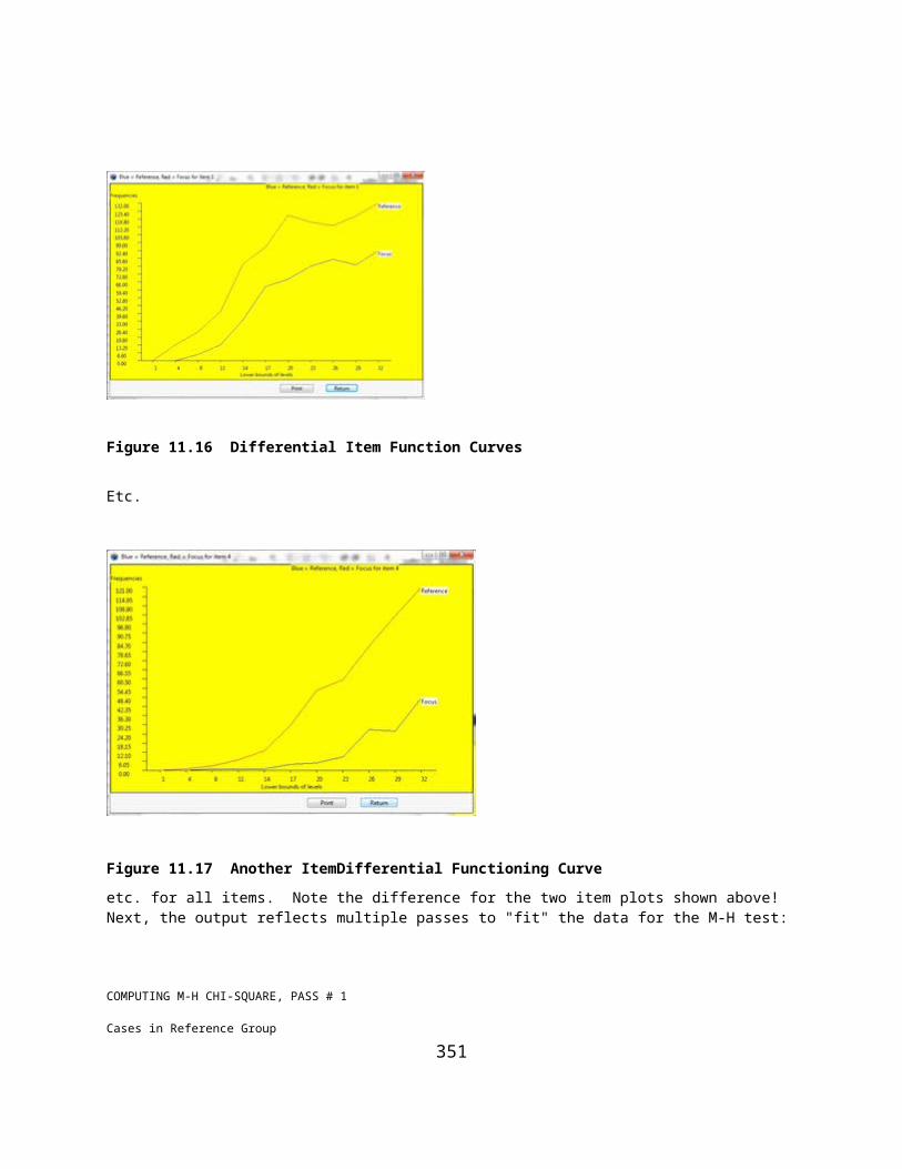
XVI The Item Banking Program
Introduction
Teachers are confronted with large classes that often make it difficult to evaluate students on the basis of evaluations based on essay examinations, problems or creative work which permits the students to demonstrate their mastery of concepts and skills in a particular area of learning. As a consequence, a variety of test questions have been devised to sample student knowledge and skills from the larger domain of knowledge contained in a given content area. Multiple choice items, true or false items, sentence completion items, matching items and short essay items have been developed to reduce the time required to evaluate students. The test theory that has evolved around these various types of items indicates that they are quite adequate in reliably assessing differences that exist among students in the domain sampled. Many states, for example, have gone to the use of computerized testing for individuals applying for driving licenses. The individual taking these examinations are presented multiple-choice types of items drawn from a computerized item bank. If the applicant performs at a given level of competence they are then permitted to demonstrate their actual driving skills in a second evaluation stage. Many Area Educational Agencies have also developed banks of items appropriate to various instructional subjects across the school grades such as in English, mathematics, science and history. Teachers may draw items from these banks to create tests over the subject area they teach.
Many teacher-constructed items utilize a picture or photograph (for example, maps, machines, paintings, etc.) as part of one or more items in a test. These pictures may be saved in the computer as “bitmap” files and tied to specific items in the bank. When the test is printed, if a picture is used it is printed prior to the printing of the item.
Item Coding
A variety of coding schemes may be developed to categorize test items. For example, one might use the Taxonomy of Educational Objectives to classify items. If one is teaching from a text book utilized across different schools in a given district, the items might be classified by the chapter, section, page and paragraph of the content to which an item refers. One may also construct a classification structure based on a breakdown of subject matter into sub-categories of the content. For example, the broad field of statistics might be initially broken down into parametric and non-parametric statistics. These domains may be further broken into categories such as univariate, multivariate, Neyman-Pearson, Bayesian, etc. which in turn may be further broken down into topics such as theory, terminology, symbols, equations, etc.
Most classification schemes result in a classification “tree” with sub-categories representing branches from the previous category level. This item banking program lets you determine your own coding system and enter codes that classify each item. You may utilize as many levels as is practical (typically three or four.) A style of code entry is required that is consistent across all items in the bank. For example, a code of 05.13.06.01 would represent a coding structure with four levels, each level having a maximum of 99 categories at each level.
In addition to classifying items by their content, one will also need to classify items by their type, that is, whether the item is a multiple-choice item, a true-false item, a matching item within a set of matching items, etc. This program requires the user to specify one of five item types for each item.
Items may also have other characteristics. In particular, one may have experience with the use of specific items in past tests and have a reasonable approximation of the difficulty of the item. Typically, the difficulty of the item is measured (in the Classical Test Theory) by the proportion of students that pass the item. For example an item with a difficulty index of .3 is more difficult than an item with an index of .8. If one is utilizing one, two or three parameter logistic scaling (Item Response Theory) he or she may have a difficulty parameter, a discrimination
351

parameter and a chance correct parameter to describe the item. In the area often called “Tailored Testing”, items are selected to administer the student in such a manner that the estimate of student ability is obtained with relatively few items. This is done by selecting items based on their difficulty parameter and the response the student gives to each item in the sequence. This program lets you enter parameter estimates (Classical or Item Response Theory estimates) for each item.
Items stored in the item bank may be retrieved on the basis of one or more criteria. One may, for example, select items within specific code areas, item difficulty and item type. By this means one can create a test of items that cover a certain topical area, have a specific range of difficulty and are of a given type or types.
352

Using the Item Bank Program
You reach the Item Banking program by clicking on the Analyses->Measurement->Item Banking menu on the main form of OpenStat. There you can click one of three choices: Enter/Edit items, Specify a Test to Administer or Generate a Test. If you click on the first submenu, you will see the following form:
Figure 16.1 The Item Bank Form
In the above form you can open a new item bank or load an existing item bank. If you create a new item bank you can enter a variety of item types into the item bank along with an estimate of the items difficulty level. Some items may have a corresponding bit map figure that you have created for the item. You can also enter a major and minor code for an item so that different tests you may want to generate have different items based on the codes selected.
Specifying a Test
If you have already created an item bank, you can then select the next option from the main menu to specify the nature of a test to generate. When you do, the following form is shown:
353

Figure 16.2 The Item Banking Test Specification Form
Within this form you can specify a test using characteristics of the items in the item bank such as the item difficulty or item codes. A test may be printed or administered on a computer screen.
Generate a Test
This is the third option in the Item Banking system. If you have specified a test the following form is displayed:
Figure 16.3 The Form to Generate a Test
354

Notice that the form first requests the name of the previously created item bank file and it then automatically loads the test specification form previously created. The sample item bank we created only contains two items which we specified to be administered on the computer screen to a student with the ID = Student 1. If we now click the “Proceed with the test button we obtain the following prompt form:
Figure 16.4 Student Verification Form for a Test Administration
When the “OK” button is pressed, the test is administered or printed. Our example would display a screen as shown below:
Figure 16.5 A Test Displayed on the Computer
Following administration of the test, the total correct score is displayed.
355

BIBLIOGRAPHY
.1. Afifi, A. A. and Azen, S. P. Statistical Analysis. A Computer Oriented Approach. New York: Academic
Press, Inc. 1972.
2. Anderberg, Michael R. Cluster Analysis for Applications. New York: Academic Press, 1973.
3. Bennett, Spencer and Bowers, David. An Introduction to Multivariate Techniques for Social and Behavioral Sciences. New York: John Wiley and Sons, Inc., 1977.
4. Besterfield, Dale H. Quality Control, 2nd Ed. Englewood Ciffs, N.J.: Prentice-Hall, Inc., 1986.
5. Bishop, Yvonne M., Fienberg, Stephen E. and Holland, Paul W. Discrete Multivariate Analysis. Theory and Practice. Cambridge, Mass.: The MIT Press 1975.
6. Blommers, Paul J. and Forsyth, Robert A. Elementary Statistical Methods in Psychology and Education, 2nd Ed. Boston, Mass.: Houghton Mifflin Company, 1977.
7. Borg, Walter R. and Gall, Meridith Damien. Educational Research. An Introduction, 5th Ed. New York: Longman, Inc., 1989.
8. Brierley, Phil. MLP neural network in C++ http://www.philbrierly.com, 2012
9. Brockwell, Peter J. and Davis, Richard A. Introduction to Time Series and Forecasting. New York: Springer-Verlag New York Inc., 1996.
10. Bruning, James L. and Kintz, B. L. Computational Handbook of Statistics, 2nd Ed. Glenview, Ill.: Scott, Foresman and Company, 1977.
11. Campbell, Donald T. and Stanley, Julian C. Experimental and Quasi-Experimental Designs for Research. Chicago, Ill.: Rand McNally College Publishing Company, 1963.
12. Chapman, Douglas G. and Schaufele, Ronald A. Elementary Probability Models and Statistical Inference. Waltham, Mass.: Ginn-Blaisdell, 1970.
13. Cody, Ronald P. and Smith, Jeffrey K. Applied Statistics and the SAS Programming Language, 4th Ed. Upper Saddle River, N.J.: Prentice Hall, 1997.
14. Cohen, Jacob and Cohen, Patricia. Applied Multiple Regression/ Correlation Analysis for the Behavioral Sciences. Hillsdale, N.J.: Lawrence Erlbaum Associates, 1975.
15. Cohen, Jacob. Statistical Power Analysis for the Behavioral Sciences, 2nd Ed., Hillsdale, N.J.: Lawrence Erlbaum Associates, 1988.
16. Comrey, Andrew L. A First Course in Factor Analysis. New York: Academic Press, Inc., 1973.
17. Cook, Thomas D. and Campbell, Donald T. Quasi-Experimentation. Design and Analysis Issues for Field Settings. Chicago, Ill.: Rand McNally College Publishing Company, 1979.
356

18. Cooley, William W. and Lohnes, Paul R. Multivariate Data Analysis. New York: John Wiley and Sons, Inc., 1971.
19. Crocker, Linda and Algina, James. Introduction to Classical and Modern Test Theory. New York: Holt, Rinehart and Winston, 1986.
20. Diekhoff, George M. Basic Statistics for the Social and Behavioral Sciences. Upper Sadle River, N.J., Prentice Hall, Inc. 1996.
21. Edwards, Allen L. Techniques of Attitude Scale Construction. New York: Appleton-Century-Crofts, Inc., 1957.
22. Efromovich, Sam. Nonparametric Curve Estimation. Methods, Theory, and Applications. New York: Springer-Verlag, 1999.
23. Ferrguson, George A. Statistical Analysis in Psychology and Education, 2nd Ed. New York: McGraw-Hill Book Company, 1966.
24. Fienberg, Stephen E. The Analysis of Cross-Classified Categorical Data, 2nd Ed. Cambridge, Mass.: The MIT Press, 1980.
25. Fox, John. Multiple and Generalized Nonparametric Regression. Thousand Oaks, Cal.: Sage Publications, Inc., 2000.
26. Freund, John E. and Walpole, Ronald E. Mathematical Statistics, 4th Ed. Englewood Cliffs, N.J.: Prentice-Hall, Inc., 1987.
27. Fruchter, Benjamin. Introduction to Factor Analysis. Princeton, N.J.: D. Van Nostrand Company, Inc., 1954.
28. Gay, L. R. Educational Research. Competencies for Analysis and Application, 4th Ed. New York: Macmillan Publishing Company, 1992.
29. Glass, Gene V. and Stanley, Julian C. Statistical Methods in Education and Psychology. Englewood Cliffs, N.J.: Prentice-Hall, Inc., 1970.
30. Gottman, John M. and Leiblum, Sandra R. How to do Psychotherapy and How to Evaluate It. A Manual for Beginners. New York: Holt, Rinehart and Winston, Inc., 1974.
31. Guertin, Wilson H. and Bailey, Jr., John P. Introduction to Modern Factor Analysis. Ann Arbor, Mich.: Edwards Brothers, Inc., 1970.
32. Gulliksen, Harold. Theory of Mental Tests. New York: John Wiley and Sons, Inc., 1950.
33. Hambleton, Ronald K. and Swaminathan, Hariharan. Item Response Theory. Principles and Applications. Boston, Mass.: Kluwer-Nijhoff Publishing, 1985.
34. Hansen, Bertrand L. and Chare, Prabhakar M. Quality Control and Applications. Englewood Cliffs, N.J.: Prentice-Hall, Inc., 1987.
35. Harman, Harry H. Modern Factor Analysis. Chicago, Ill.: The University of Chicago Press, 1960.
36. Hays, William L. Statistics for Psychologists. New York: Holt, Rinehart and Winston, Inc., 1963.
357

37. Heise, David R. Causal Analysis. New York: John Wiley and Sons, Inc., 1975.
38. Hinkle, Dennis E., Wiersma, William and Jurs, Stephen G. Applied Statistics for the Behavioral Sciences, 2nd Edition. Boston, Mass.: Houghton Mifflin Company, 1988.
39. Huntsberger, David H. and Billingsley, Patrick. Elements of Statistical Inference, 6th Ed. Boston, Mass.: Allyn and Bacon, Inc., 1987.
40. Kelly, Louis G. Handbook of Numerical Methods and Applications. Reading, Mass.: Addison-Wesley Publishing Company, 1967.
41. Kennedy, Jr., William J. and Gentle, James E. Statistical Computing. New York: Marcel Dekker, Inc., 1980.
42. Kerlinger, Fred N. and Pedhazur, Elazar J. Multiple Regression in Behavioral Research. New York: Holt, Rinehart and Winston, Inc., 1973.
43. Lieberman, Bernhardt (Editor). Contemporary Problems in Statistics. A book of Readings for the Behavioral Sciences. New York: Oxford University Press, 1971.
44. Lindgren, B. W. and McElrath, G. W. Introduction to Probability and Statistics, 2nd Ed. New York: The Macmillan Company, 1966.
45. Marcoulides, George A. and Schumacker, Randall E. (Editors). Advanced Structural Equation Modeling. Issues and Techniques. Mahwah, N.J.: Lawrence Erlbaum Associates, 1996.
46. Masters, Timothy. Practical Neural Network Recipes in C++. San Diego, Calif.: Morgan Kaufmann, 1993.
47. McNeil, Keith, Newman, Isadore and Kelly, Francis J. Testing Research Hypotheses with the General Linear Model. Carbondale, Ill.: Southern Illinois University Press, 1996.
48. McNemar, Quinn. Psychological Statistics, 4th Ed. New York: John Wiley and Sons, Inc., 1969.
49. Minium, Edward W. Statistical Reasoning in Psychology and Education, 2nd Ed. New York: John Wiley and Sons, Inc., 1978.
50. Montgomery, Douglas C. Statistical Quality Control. New York: John Wiley and Sons, Inc., 1985.
51. Mulaik, Stanley A. The Foundations of Factor Analysis. New York: McGraw-Hill Book Company, 1972.
52. Myers, Jerome L. Fundamentals of Experimental Design. Boston, Mass.: Allyn and Bacon, Inc., 1966.
53. Nunnally, Jum C. Psychometric Theory. New York: McGraw-Hill Book Company, Inc., 1967.
54. Olson, Chester L. Essentials of Statistics. Making Sense of Data. Boston, Mass.: Allyn and Bacon, Inc., 1987.
55. Payne, David A., Editor. Curriculum Evaluation. Commentaries on Purpose, Process, Product. Lexington, Mass.: D. C. Heath and Company, 1974.
56. Pedhazur, Elazar J. Multiple Regression in Behavioral Research. Explanation and Prediction. 3rd Ed. Fort Worth, Texas: Holt, Rinehart and Winston, Inc., 1997.
358

57. Press, William H., Flannery, Brian P., Teukolsky, Saul A., and Vetterling, William T. Numerical Recipes in C. The Art of Scientific Computing. Cambridge University Press, 1988.
58. Ralston, Anthony and Wilf, Herbert S. Mathematical Methods for Digital Computers. New York: John Wiley and Sons, Inc., 1966.
59. Rich, Elain and Knight, Kevin. Artificial Intelligence. McGraw-Hill, Inc., 1983.
60. Rao, C. Radhakrishna. Linear Statistical Inference and Its Applications. New York: John Wiley and Sons, Inc., 1965.
61. Rao, Valluru and Rao, Hayagriva. C++ Neural Networks and Fuzzy Logic, 2nd Ed. New York: MIS Press, 1995.
62. Rogers, Joey. Object-Oriented Neural Networks in C++. San Diego, Calif.: Academic Press, 1997.
63. Roscoe, John T. Fundamental Research Statistics for the Behavioral Sciences, 2nd Ed. New York: Holt, Rinehart and Winston, Inc., 1975.
64. Rummel, R. J. Applied Factor Analysis. Evanston, Ill.: Northwestern University Press, 1970.
65. Scheffe', Henry. The Analysis of Variance. New York: John Wiley and Sons, Inc., 1959.
66. Schumacker, Randall E. and Lomax, Richard G. A Beginner's Guide to Structural Equation Modeling. Mahwah, N.J.: Lawrence Erlbaum Associates, 1996.
67. Siegel, Sidney. Nonparametric Statistics for the Behavioral Sciences. New York: McGraw-Hill Book Company, Inc., 1956.
68. Silverman, Eliot N. and Brody, Linda A. Statistics. A Common Sense Approach. Boston, Mass.: Prindle, Weber and Schmidt, Inc., 1973.
69. SPSS, Inc. SPSS-X User's Guide, 3rd Ed. Chicago, Ill.: SPSS, Inc., 1988.
70. Steele, Sara M. Contemporary Approaches to Program Evaluation: Implications for Evaluating Programs for Disadvantaged Adults. Syracuse, New York: ERIC Clearinghouse on Adult Education (undated).
71. Stevens, James. Applied Multivariate Statistics for the Social Sciences, 3rd Ed. Mahwah, N.J.: Lawrence Erlbaum Associates, 1996.
72. Stodala, Quentin and Stordahl, Kalmer. Basic Educational Tests and Measurement. Chicago, Ill.: Science Research Associates, Inc., 1967.
73. Thomson, Godfrey. The Factorial Analysis of Human Ability, 5th Ed., Boston, Mass.: Houghton Mifflin Company, 1951.
74. Thorndike, Robert L. Applied Psychometrics. Boston, Mass.: Houghton Mifflin Company, 1982.
75. Thorndike, Robert L. (Editor.) Educational Measurement, 2nd Edition. One Dupont Circle, Washington D.C.: American Council on Education, 1971.
76. Veldman, Donald J. Fortran Programming for the Behavioral Sciences. Holt, Rinehart and Winston, New York, 1967, pages 308-317.
359

77. Walker, Helen M. and Lev, Joseph. Statistical Inference. New York: Henry Holt and Company, 1953.
78. Winer, B. J. Statistical Principles in Experimental Design. New York: McGraw-Hill Book Company, Inc., 1962.
79. Worthen, Blaine R. and Sanders, James R. Educational Evaluation: Theory and Practice. Belmont, Calif.: Wadsworth Publishing Company, Inc., 1973.
80. Yamane, Taro. Mathematics for Economists. An Elementary Survey. Englewood Cliffs, N.J.: Prentice-Hall, Inc., 1962.
360
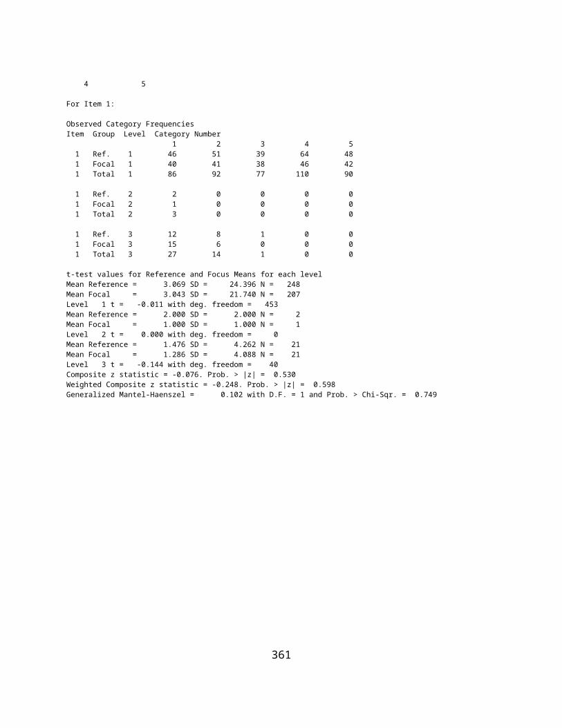
INDEX
/ Recode option, 262 or 3 Way Fixed ANOVA with 1 case per cell, 1312-Stage Least-Squares Regression, 161Adjustment of Reliability For Variance Change, 304Analyses Menu, 27Analysis of Variance, 84Analysis of Variance - Treatments by Subjects Design, 88Analysis of Variance Using Multiple Regression Methods, 137Auto and Partial Autocorrelation, 76auto-correlation, 70Autocorrelation, 70auto-correlations, 76Average Linkage Hierarchical Cluster Analysis, 186AxB Log Linear Analysis, 222AxBxC Log Linear Analysis, 225Bartlett Chi-square test for homogeneity, 85Bartlett Test of Sphericity, 214binary files, 15Binary Logistic Regression, 151Box plots, 39Box Plots, 39Breakdown, 37Breakdown Procedure, 31Bubble Plot, 54Canonical Correlations, 147Cluster Analyses, 179Cochran Q Test, 252Comma separated field files, 15Common Errors, 28Compare Observed to a Theoretical Distribution, 60Comparison of Two Sample Means, 82Contingency Chi-Square, 242Correlations in Dependent Samples, 67Correspondence Analysis, 216Cox Proportional Hazards Survival Regression, 153Creating a File, 15Cross-Tabulation, 35CUSUM Chart, 323data smoothing, 70Defect (Non-conformity) c Chart, 327Defects Per Unit u Chart, 329Differential Item Functioning, 289Discriminant Function / MANOVA, 171Distribution Parameter Estimates, 30Distribution Plots, 31Eigenvalues and Vectors, 350
Entering Data, 17Epidata files, 15Factor Analysis, 198Files, 15Fisher’s Exact Test, 247Fixed Format files, 15Frequencies, 32Friedman Two Way ANOVA, 254Generate Test Data, 311Guttman Scalogram Analysis, 286Hartley Fmax test, 85Help, 19Hierarchical Cluster Analysis, 179Hoyt Reliability, 278Installing OpenStat, 13Item Analysis, 272Item Banking, 358Kaplan-Meier Survival Test, 261Kendall’s Coefficient of Concordance, 248Kendall's Tau and Partial Tau, 259K-Means Clustering Analysis, 184Kruskal-Wallis One-Way ANOVA, 249Kuder-Richardson #21 Reliability, 280Latin and Greco-Latin Square Designs, 104Linear Programming, 331Log Linear Screening, 220Mann-Whitney U Test, 245Matrix files, 15Matrix Operations, 345Median Polish Analysis, 213Microsoft Excel, 22Multiple Groups X versus Y Plot, 61Nested Factors Analysis Of Variance, 99Non-Linear Regression, 166Normality Tests, 50Observed and Theoretical Distributions, 48One Sample Tests, 77One, Two or Three Way ANOVA, 84Options menu, 16p Chart, 325Partial and Semi_Partial Correlations, 68partial auto-correlation, 75partial auto-correlations, 76Path Analysis, 189Pie Chart, 45Polynomial Regression Smoothing, 72Polytomous DIF Analysis, 307Probability of a Binomial Event, 256
361

Product Moment Correlation, 63Proportion Differences, 79QQ and PP Plots, 49Random Selection, 25Range Chart, 318Rasch One Parameter Item Analysis, 282Resistant Line, 52Runs Test, 257S Control Chart, 320Saving a File, 18select a specified range of cases, 26Select Cases, 23, 24Select If, 25Sign Test, 253Simple Linear Regression, 65Simulation Menu, 27Single Sample Proportion Test, 78Single Sample Variance Test, 79Smooth Data, 56Sort, 22Space separated field files, 15Spearman Rank Correlation, 244Spearman-Brown Reliability Prophecy, 314Stem and Leaf Plot, 47String labels, 28Successive Interval Scaling, 287Sums of Squares by Regression, 142
SVDInverse, 346Tab separated field f, 15Testing Equality of Correlations, 66Text files, 15the AxS ANOVA, 90The General Linear Model, 146The GradeBook, 354The Kolmogorov-Smirnov Test, 268The Options Form, 17The Variables Equation Option, 21The Variables Menu, 19Three Factor Nested ANOVA, 101Three Variable Rotation, 42t-test, 81t-Tests, 81Two Factor Repeated Measures Analysis, 93Two Within Subjects ANOVA, 134Using MatMan, 335Variable Transformation, 20Variables Definition, 16Weighted Composite Test Reliablity, 281Weighted Least-Squares Regression, 155Wilcoxon Matched-Pairs Signed Ranks Test, 251X Versus Multiple Y Plot, 58X Versus Y Plots, 43XBAR Chart, 315
362


![Table of Contents - MicroImages, Inc. · Table of Contents Introduction 7 Editorial and Associated News [by Dr. Lee D. Miller, President] 9 ... Enhanced Sketch Annotation Setting](https://img.pdfslide.us/doc/110x75/5f0260a17e708231d403f92e/table-of-contents-microimages-inc-table-of-contents-introduction-7-editorial.jpg)