· Abstract. We investigate the three-dimensional interior and exterior Neumann-type boundary-value problems of statics of the thermo-electro-magneto-elasticity theory

Memoirs on Differential Equations and Mathematical PhysicsVolume 53, 2011, 99–126

M. Mrevlishvili and D. Natroshvili

INVESTIGATION OF INTERIOR ANDEXTERIOR NEUMANN-TYPE STATICBOUNDARY-VALUE PROBLEMSOF THERMO-ELECTRO-MAGNETOELASTICITY THEORY

Abstract. We investigate the three-dimensional interior and exteriorNeumann-type boundary-value problems of statics of the thermo-electro-magneto-elasticity theory. We construct explicitly the fundamental matrixof the corresponding strongly elliptic non-self-adjoint 6× 6 matrix differen-tial operator and study their properties near the origin and at infinity. Weapply the potential method and reduce the corresponding boundary-valueproblems to the equivalent system of boundary integral equations. We havefound efficient asymptotic conditions at infinity which ensure the unique-ness of solutions in the space of bounded vector functions. We analyzethe solvability of the resulting boundary integral equations in the Holderand Sobolev-Slobodetski spaces and prove the corresponding existence the-orems. The necessary and sufficient conditions of solvability of the interiorNeumann-type boundary-value problem are written explicitly.

2010 Mathematics Subject Classification. 35J57, 74F05, 74F15,74B05.

Key words and phrases. Thermo-electro-magneto-elasticity, boun-dary-value problem, potential method, boundary integral equations, unique-ness theorems, existence theorems.

îâäæñéâ. ïðŽðæŽöæ àŽéëçãèâñèæŽ êâæéŽêæï öæàŽ áŽ àŽîâ ïŽéàŽêäëéæ-èâĲæŽêæ ŽéëùŽêâĲæ åâîéë-âèâóðîë-éŽàêâðë áîâçŽáëĲæï åâëîææï ïðŽðæçæïàŽêðëèâĲâĲæïŽåãæï. öâïŽĲŽéæïæ ëìâîŽðëîæïŽåãæï, îëéâèæù ûŽîéëŽáàâêï6 × 6 àŽêäëéæèâĲæï éŽðîæùñè ŽîŽåãæåöâñôèâĲñè, úèæâîŽá âèæòïñî áæ-òâîâêùæŽèñî ëìâîŽðëîï, ùýŽáæ ïŽýæåŽŽ ŽàâĲñèæ òñêáŽéâêðñî ŽéëêŽýïêåŽéŽðîæùŽ áŽ áŽáàâêæèæŽ éæïæ Žïæéìðëðñîæ åãæïâĲâĲæ ïŽåŽãæïŽ áŽ ñïŽïîñ-èëĲæï éæáŽéëöæ. ìëðâêùæŽèåŽ éâåëáæï àŽéëõâêâĲæå ïŽïŽäôãîë ŽéëùŽêâ-Ĳæ áŽõãŽêæèæŽ âçãæãŽèâêðñî ïŽïŽäôãîë æêðâàîŽèñî (òïâãáëáæòâîâêùæ-Žèñî) àŽêðëèâĲŽåŽ ïæïðâéŽäâ. àŽéëçãèâñèæŽ Žé æêðâàîŽèñîæ àŽêðëèâĲæïŽéëýïêŽáëĲæï ïŽçæåýæ áŽ áŽéðçæùâĲñèæŽ öâïŽĲŽéæïæ ïŽïŽäôãîë ŽéëùŽêâĲæïŽéëêŽýïêâĲæï ŽîïâĲëĲæï åâëîâéâĲæ ßâèáâîæïŽ áŽ ïëĲëèâãïèëĲëáâùçæïòñêóùæñî ïæãîùââĲöæ. ŽôïŽêæöêŽãæŽ, îëé ùýŽáæ ïŽýæåŽŽ Žéëûâîæèæ êâæéŽêæïöæàŽ ŽéëùŽêæï ŽîïâĲëĲæï ŽñùæèâĲâèæ áŽ ïŽçéŽîæïæ ìæîëĲâĲæ.

Einvestigation of Interior and Exterior Neumann-Type 101

1. Introduction

Modern industrial and technological processes apply widely, on the onehand, composite materials with complex microstructure and, on the otherhand, complex composed structures consisting of materials having essen-tially different physical properties (for example, piezoelectric, piezomag-netic, hemitropic materials, two- and multi-component mixtures, nano-materials, bio-materials, and solid structures constructed by composition ofthese materials, such as, e.g., Smart Materials and other meta-materials).Therefore the investigation and analysis of mathematical models describingthe mechanical, thermal, electric, magnetic and other physical properties ofsuch materials have a crucial importance for both fundamental research andpractical applications. In particular, the investigation of correctness of cor-responding mathematical models (namely, existence, uniqueness, smooth-ness, asymptotic properties and stability of solutions) and construction ofappropriate adequate numerical algorithms have a crucial role for funda-mental research.

In the study of active material systems, there is significant interest in thecoupling effects between elastic, electric, magnetic and thermal fields. Themathematical model of statics of the thermo-electro-magneto-elasticity the-ory is described by the non-self-adjoint 6× 6 system of second order partialdifferential equations with appropriate boundary conditions. The problemis to determine three components of the elastic displacement vector, theelectric and magnetic scalar potential functions and the temperature dis-tribution. Other field characteristics (e.g., mechanical stresses, electric andmagnetic fields, electric displacement vector, magnetic induction vector, andheat flux vector) can be then determined by the gradient and constitutiveequations (for details see [2], [3], [4], [5], [6], [16], [21], [24], [27]).

For the equations of dynamics the uniqueness theorems of solutions forsome initial-boundary-value problems are well studied. In particular, in thereference [16] the uniqueness theorem is proved without making restrictionson the positive definiteness on the elastic moduli, while the uniqueness theo-rems for the basic boundary-value problems (BVP) of statics of the thermo-electro-magneto-elasticity theory are proved in [20]. Existence theorems forthe Dirichlet-type boundary-value problems are established in [19]. To thebest of our knowledge, the existence of solutions to the Neumann-type BVPsof statics are not treated in the scientific literature.

In this paper, with the help of the potential method we reduce the three-dimensional interior and exterior Neumann-type boundary-value problemsof the thermo-electro-magneto-elasticity theory to the equivalent 6× 6 sys-tems of integral equations and analyze their solvability in the Holder andSobolev-Slobodetski spaces and prove the corresponding uniqueness and ex-istence theorems.

Essential difficulties arise in the study of exterior BVPs for unboundeddomains. The case is that one has to consider the problem in a class of

102 M. Mrevlishvili and D. Natroshvili

vector functions which are bounded at infinity. This complicates the proofof uniqueness and existence theorems since Green’s formulas do not holdfor such vector functions and analysis of null spaces of the correspondingintegral operators needs special consideration. We have found efficient andnatural asymptotic conditions at infinity which ensure the uniqueness of so-lutions in the space of bounded vector functions. Moreover, for the interiorNeumann-type boundary-value problem, the complete system of linearlyindependent solutions of the corresponding homogeneous adjoint integralequation is constructed in polynomials and the necessary and sufficient con-ditions of solvability of the problem are written explicitly.

2. Formulation of Problems

Here we collect the basic field equations of the thermo-electro-magneto-elasticity theory and formulate the interior and exterior Neumann-typeboundary-value problems of statics.

2.1. Field equations. Throughout the paper u = (u1, u2, u3)> denotes thedisplacement vector, σij is the mechanical stress tensor, εkj = 2−1(∂kuj +∂juk) is the strain tensor, the vectors E = (E1, E2, E3)> and H =(H1,H2,H3)> are electric and magnetic fields respectively, D=(D1,D2,D3)>

is the electric displacement vector and B = (B1, B2, B3)> is the mag-netic induction vector, ϕ and ψ stand for the electric and magnetic po-tentials and E = − gradϕ, H = − gradψ, ϑ is the temperature increment,q = (q1, q2, q3)> is the heat flux vector, and S is the entropy density.

We employ also the notation ∂ = ∂x = (∂1, ∂2, ∂3), ∂j = ∂/∂xj , ∂t =∂/∂t; the superscript (·)> denotes transposition operation. In what followsthe summation over the repeated indices is meant from 1 to 3, unless statedotherwise.

In this subsection we collect the field equations of the linear theory ofthermo-electro-magneto-elasticity for a general anisotropic case and intro-duce the corresponding matrix partial differential operators. To this end,we recall here the basic relations of the theory:

Constitutive relations:

σrj = σjr = crjklεkl − elrjEl − qlrjHl − λrjϑ, r, j = 1, 2, 3, (2.1)

Dj = ejklεkl + κjlEl + ajlHl + pjϑ, j = 1, 2, 3, (2.2)

Bj = qjklεkl + ajlEl + µjlHl + mjϑ, j = 1, 2, 3, (2.3)

S = λklεkl + pkEk + mkHk + γϑ. (2.4)

Fourier Law:qj = −ηjl∂lϑ, j = 1, 2, 3. (2.5)

Equations of motion:

∂jσrj + Xr = %∂2t ur, r = 1, 2, 3. (2.6)


Quasi-static equations for electro-magnetic fields where the rate of magneticfield is small (electric field is curl free) and there is no electric current(magnetic field is curl free):

∂jDj = %e, ∂jBj = 0. (2.7)

Linearized equation of the entropy balance:

T0∂tS −Q = −∂jqj . (2.8)

Here % is the mass density, %e is the electric density, crjkl are the elasticconstants, ejkl are the piezoelectric constants, qjkl are the piezomagneticconstants, κjk are the dielectric (permittivity) constants, µjk are the mag-netic permeability constants, ajk are the coupling coefficients connectingelectric and magnetic fields, pj and mj are constants characterizing the re-lation between thermodynamic processes and electromagnetic effects, λjk

are the thermal strain constants, ηjk are the heat conductivity coefficients,γ = %cT−1

0 is the thermal constant, T0 is the initial reference tempera-ture, that is the temperature in the natural state in the absence of de-formation and electromagnetic fields, c is the specific heat per unit mass,X = (X1, X2, X3)> is a mass force density, Q is a heat source intensity.

The constants involved in these equations satisfy the symmetry condi-tions:

crjkl = cjrkl = cklrj , eklj = ekjl,

qklj = qkjl, κkj = κjk, λkj = λjk,

µkj = µjk, ηkj = ηjk, akj = ajk,

r, j, k, l = 1, 2, 3. (2.9)

From physical considerations it follows that (see, e.g., [16], [27]):

crjklξrjξkl ≥ c0ξklξkl, κkjξkξj ≥ c1|ξ|2,µkjξkξj ≥ c2|ξ|2, ηkjξkξj ≥ c3|ξ|2,

for all ξkj = ξjk ∈ R and for all ξ = (ξ1, ξ2, ξ3) ∈ R3,

(2.10)

where c0, c1, c2, and c3 are positive constants.It is easy to see that due to the symmetry conditions (2.9)

crjklξrjξkl ≥ c0ξklξkl, κkjξkξj ≥ c1|ξ|2,µkjξkξj ≥ c2|ξ|2, ηkjξkξj ≥ c3|ξ|2,

for all ξkj = ξjk ∈ C and for all ξ = (ξ1, ξ2, ξ3) ∈ C3.

More careful analysis related to the positive definiteness of the potentialenergy and thermodynamical laws insure that for arbitrary ζ ′, ζ ′′ ∈ C3 andθ ∈ C there is a positive constant δ0 depending on the material constantssuch that (cf. [27])

κkjζ′kζ ′j + akj

(ζ ′kζ ′′j + ζ ′kζ ′′j

)+ µkjζ

′′k ζ ′′j ± 2<[

θ(pjζ′j + mjζ

′′j )

]+ γ|θ|2 ≥

≥ δ0

(|ζ ′|2 + |ζ ′′|2 + |θ|2). (2.11)


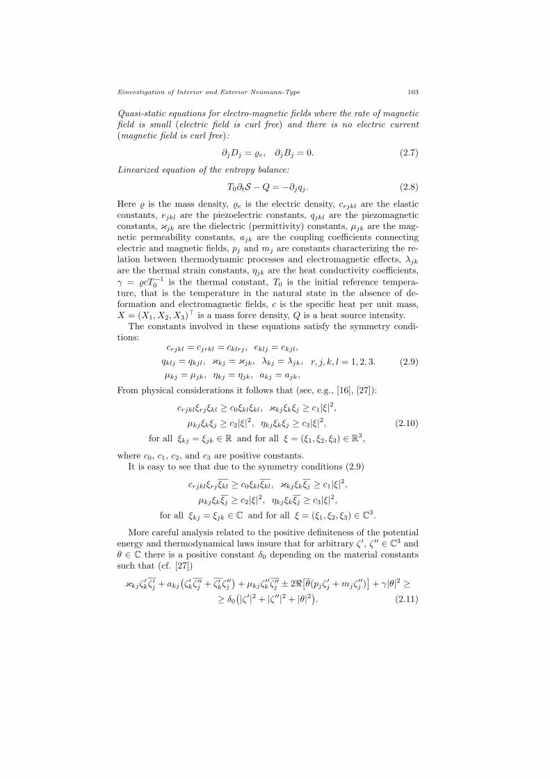
This condition is equivalent to positive definiteness of the matrix

Ξ :=

[κkj ]3×3 [akj ]3×3 [pj ]3×1

[akj ]3×3 [µkj ]3×3 [mj ]3×1

[pj ]1×3 [mj ]1×3 γ

7×7

.

In particular, it follows that the matrix

Λ :=

[[κkj ]3×3 [akj ]3×3

[akj ]3×3 [µkj ]3×3

]

6×6

(2.12)

is positive definite, i.e.,

κkjζ′kζ ′j + akj

(ζ ′kζ ′′j + ζ ′kζ ′′j

)+ µkjζ

′′k ζ ′′j ≥ κ(|ζ ′|2 + |ζ ′′|2)

with some positive constant κ depending on the material parameters in-volved in (2.12). A sufficient condition for the quadratic form in the lefthand side of (2.11) to be positive definite then reads as ν2 < κγ

6 withν = max

|p1|, |p2|, |p3|, |m1|, |m2|, |m3|.

With the help of the symmetry conditions (2.9) we can rewrite the con-stitutive relations (2.1)–(2.4) as follows

σrj = crjkl∂luk + elrj∂lϕ + qlrj∂lψ − λrjϑ, r, j = 1, 2, 3,

Dj = ejkl∂luk − κjl∂lϕ− ajl∂lψ + pjϑ, j = 1, 2, 3,

Bj = qjkl∂luk − ajl∂lϕ− µjl∂lψ + mjϑ, j = 1, 2, 3,

S = λkl∂luk − pl∂lϕ−ml∂lψ + γϑ.

In the theory of thermo-electro-magneto-elasticity the components of thethree-dimensional mechanical stress vector acting on a surface element witha unit normal vector n = (n1, n2, n3) have the form

σrjnj = crjklnj∂luk + elrjnj∂lϕ + qlrjnj∂lψ − λrjnjϑ, r = 1, 2, 3,

while the normal components of the electric displacement vector, magneticinduction vector and heat flux vector read as

Djnj = ejklnj∂luk − κjlnj∂lϕ− ajlnj∂lψ + pjnjϑ,

Bjnj = qjklnj∂luk − ajlnj∂lϕ− µjlnj∂lψ + mjnjϑ,

qjnj = −ηjlnj∂lϑ.

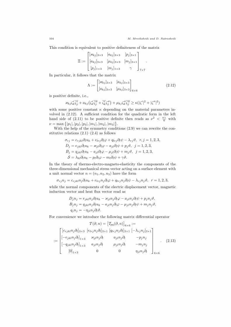
For convenience we introduce the following matrix differential operator

T (∂, n) =[Tpq(∂, n)

]6×6

:=

:=

[crjklnj∂l]3×3 [elrjnj∂l]3×1 [qlrjnj∂l]3×1 [−λrjnj ]3×1

[−ejklnj∂l]1×3 κjlnj∂l ajlnj∂l −pjnj

[−qjklnj∂l]1×3 ajlnj∂l µjlnj∂l −mjnj

[0]1×3 0 0 ηjlnj∂l

6×6

. (2.13)


Evidently, for a six vector U := (u, ϕ, ψ, ϑ)> we have

T (∂, n)U =(σ1jnj , σ2jnj , σ3jnj ,−Djnj ,−Bjnj ,−qjnj

)>. (2.14)

The components of the vector T U given by (2.14) have the following physicalsense: the first three components correspond to the mechanical stress vectorin the theory of thermo-electro-magneto-elasticity, the forth, fifth and sixthones are respectively the normal components of the electric displacementvector, magnetic induction vector and heat flux vector with opposite sign.

As we see, all the thermo-mechanical and electro-magnetic characteristicscan be determined by the six functions: the three displacement componentsuj , j = 1, 2, 3, temperature distribution ϑ, and the electric and magneticpotentials ϕ and ψ. Therefore, all the above field relations and the cor-responding boundary-value problems we reformulate in terms of these sixfunctions.

First of all from the equations (2.1)–(2.8) we derive the basic linear sys-tem of dynamics of the theory of thermo-electro-magneto-elasticity:

crjkl∂j∂luk(x, t) + elrj∂j∂lϕ(x, t) + qlrj∂j∂lψ(x, t)− λrj∂jϑ(x, t)−−%∂2

t ur(x, t) = −Xr(x, t), r = 1, 2, 3,

−ejkl∂j∂luk(x, t)+κjl∂j∂lϕ(x, t)+ajl∂j∂lψ(x, t)−pj∂jϑ(x, t)=−%e(x, t),

−qjkl∂j∂luk(x, t) + ajl∂j∂lϕ(x, t) + µjl∂j∂lψ(x, t)−mj∂jϑ(x, t) = 0,

−T0λkl∂t∂luk(x, t) + T0pl∂t∂lϕ(x, t) + T0ml∂t∂lψ(x, t) + ηjl∂j∂lϑ(x, t)−−T0γ∂tϑ(x, t) = −Q(x, t).

If all the functions involved in these equations are harmonic time dependent,that is they can be represented as the product of a function of the spatialvariables (x1, x2, x3) and the multiplier expτt, where τ = σ+ iω is a com-plex parameter, we have then the pseudo-oscillation equations of the theoryof thermo-electro-magneto-elasticity. Note that the pseudo-oscillation equa-tions can be obtained from the corresponding dynamical equations by theLaplace transform. If τ is a pure imaginary number, τ = iω with the socalled frequency parameter ω ∈ R, we obtain the steady state oscillationequations. Finally, if τ = 0 we get the equations of statics:

crjkl∂j∂luk(x) + elrj∂j∂lϕ(x) + qlrj∂j∂lψ(x)− λrj∂jϑ(x) =

= −Xr(x), r = 1, 2, 3,

−ejkl∂j∂luk(x) + κjl∂j∂lϕ(x) + ajl∂j∂lψ(x)− pj∂jϑ(x) = −%e(x),

−qjkl∂j∂luk(x) + ajl∂j∂lϕ(x) + µjl∂j∂lψ(x)−mj∂jϑ(x) = 0,

ηjl∂j∂lϑ(x) = −Q(x).

(2.15)

In matrix form these equations can be written as

A(∂)U(x) = Φ(x),

where

U = (u1, u2, u3, u4, u5, u6)> := (u, ϕ, ψ, ϑ)>,


Φ = (Φ1, . . . , Φ6)> := (−X1,−X2,−X3,−%e, 0,−Q)>,

and A(∂) is the matrix differential operator generated by equations (2.15),

A(∂) = [Apq(∂)]6×6 :=

:=

[crjkl∂j∂l]3×3 [elrj∂j∂l]3×1 [qlrj∂j∂l]3×1 [−λrj∂j ]3×1

[−ejkl∂j∂l]1×3 κjl∂j∂l ajl∂j∂l −pj∂j

[−qjkl∂j∂l]1×3 ajl∂j∂l µjl∂j∂l −mj∂j

[0]1×3 0 0 ηjl∂j∂l

6×6

. (2.16)

2.2. Formulation of the boundary-value problems. Let Ω+ be a boun-ded domain in R3 with a smooth boundary S = ∂Ω+, Ω+ = Ω+ ∪ S, andΩ− := R3 \ Ω+. Assume that the domains Ω± are filled by an anisotropichomogeneous material with thermo-electro-magneto-elastic properties.

Throughout the paper n = (n1, n2, n3) stands for the outward unit nor-mal vector with respect to Ω+ at the point x ∈ ∂Ω+.

Neumann-type problems (N)±: Find a regular solution vector U =(u,ϕ,ψ,ϑ)> ∈ [C1(Ω+)]6 ∩ [C2(Ω+)]6 (resp. U ∈ [C1(Ω−)]6 ∩ [C2(Ω−)]6), tothe system of equations

A(∂)U = Φ in Ω±,

satisfying the Neumann-type boundary conditionsT U

± = f on S,

where A(∂) is a nonselfadjoint strongly elliptic matrix partial differential op-erator generated by the equations of statics of the theory of thermo-electro-magneto-elasticity defined in (2.16), while T (∂, n) is the matrix boundaryoperator defined in (2.13). The symbols ·± denote the one sided limits(the trace operators) on ∂Ω± from Ω±.

In our analysis we need special asymptotic conditions at infinity in thecase of unbounded domains [20].

Definition 2.1. We say that a continuous vector U = (u, ϕ, ψ, ϑ)> ≡(U1, · · · , U6)> in the domain Ω− has the property Z(Ω−) if the followingconditions are satisfied

U(x) := (u(x), ϕ(x), ψ(x))> = O(1),

U6(x) = ϑ(x) = O(|x|−1),as |x| → ∞,

limR→∞

14πR2

∫

ΣR

Uk(x) dΣR = 0, k = 1, 5,

where ΣR is a sphere centered at the origin and radius R.

In what follows we always assume that in the case of exterior boundary-value problem a solution possesses Z(Ω−) property.


2.3. Potentials and their properties. Denote by Γ(x) = [Γkj(x)]6×6 thematrix of fundamental solutions of the operator A(∂), A(∂)Γ(x) = I6 δ(x),where δ(·) is the Dirac’s delta distribution and I6 stands for the unit 6× 6matrix. Applying the generalized Fourier transform technique, the funda-mental matrix can be constructed explicitly,

Γ(x) = F−1ξ→x[A−1(−i ξ)] , (2.17)

where F−1 is the generalized inverse Fourier transform and A−1(−i ξ) isthe matrix inverse to A(−i ξ). The properties of the fundamental matrixnear the origin and at infinity are established in [23]. The entries of thefundamental matrix Γ(x) are homogeneous functions in x and at the originand at infinity the following asymptotic relations hold

Γ(x) =

[[O(|x|−1)]5×5 [O(1)]5×1

[0]1×5 O(|x|−1)

]

6×6

.

Moreover, the columns of the matrix Γ(x) possess the property Z(R3 \0).With the help of the fundamental matrix we construct the generalized singleand double layer potentials, and the Newton-type volume potentials,

V (h)(x) =∫

S

Γ(x− y)h(y) dSy, x ∈ R3 \ S,

W (h)(x) =∫

S

[P(∂y, n(y))Γ>(x− y)]> h(y) dSy, x ∈ R3 \ S,

NΩ±(g)(x) =∫

Ω±

Γ(x− y) g(y) dy, x ∈ R3,

where S = ∂Ω± ∈ Cm, κ with integer m ≥ 1 and 0 < κ ≤ 1; h =(h1, . . . , h6)> and g = (g1, · · · , g6)> are density vector-functions defined re-spectively on S and in Ω±; the so called generalized stress operator P(∂, n),associated with the adjoint differential operator A∗(∂) = A>(−∂), reads as

P(∂, n) =[Ppq(∂, n)

]6×6

=

=

[crjklnj∂l]3×3 [−elrjnj∂l]3×1 [−qlrjnj∂l]3×1 [0]3×1

[ejklnj∂l]1×3 κjlnj∂l ajlnj∂l 0

[qjklnj∂l]1×3 ajlnj∂l µjlnj∂l 0

[0]1×3 0 0 ηjlnj∂l

. (2.18)

The following properties of layer potentials immediately follow from theirdefinition.

Theorem 2.2. The generalized single and double layer potentials solvethe homogeneous differential equation A(∂)U = 0 in R3 \S and possess theproperty Z(Ω−).


In what follows by Lp, W rp , Hs

p , and Bsp,q (with r ≥ 0, s ∈ R, 1 < p < ∞,

1 ≤ q ≤ ∞) we denote the well-known Lebesgue, Sobolev–Slobodetski,Bessel potential, and Besov function spaces, respectively (see, e.g., [29]).Recall that Hr

2 = W r2 = Br

2,2, Hs2 = Bs

2,2, W tp = Bt

p,p, and Hkp = W k

p , forany r ≥ 0, for any s ∈ R, for any positive and non-integer t, and for anynon-negative integer k.

With the help of Green’s formulas, one can derive general integral repre-sentations of solutions to the homogeneous equation A(∂)U = 0 in Ω±. Inparticular, the following theorems hold.

Theorem 2.3. Let S = ∂Ω+ ∈ C1,κ with 0 < κ ≤ 1 and U be aregular solution to the homogeneous equation A(∂)U = 0 in Ω+ of the class[C1(Ω+)]6∩[C2(Ω+)]6. Then there holds the integral representation formula

W (U+)(x)− V (T U+)(x) =

U(x) for x ∈ Ω+,

0 for x ∈ Ω−.

Theorem 2.4. Let S = ∂Ω− be C1,κ-smooth with 0 < κ ≤ 1 and let Ube a regular solution to the homogeneous equation A(∂)U = 0 in Ω− of theclass [C1(Ω−)]6 ∩ [C2(Ω−)]6 having the property Z(Ω−). Then there holdsthe integral representation formula

−W (U−)(x) + V (T U−)(x) =

0 for x ∈ Ω+,

U(x) for x ∈ Ω−.

By standard limiting procedure, these formulas can be extended to Lip-schitz domains and to solution vectors from the spaces [W 1

p (Ω+)]6 and[W 1

p,loc(Ω−)]6 ∩ Z(Ω−) with 1 < p < ∞ (cf., [12], [17], [25]).

The qualitative and mapping properties of the layer potentials are de-scribed by the following theorems (cf. [7], [9], [15], [17], [23]).

Theorem 2.5. Let S = ∂Ω± ∈ Cm,κ with integers m ≥ 1 and k ≤m− 1, and 0 < κ′ < κ ≤ 1. Then the operators

V : [Ck,κ′(S)]6→ [Ck+1,κ′(Ω±)]6, W : [Ck,κ′(S)]6→ [Ck,κ′(Ω±)]6 (2.19)

are continuous.For any g ∈ [C0,κ′(S)]6, h ∈ [C1,κ′(S)]6, and any x ∈ S we have the

following jump relations:

V (g)(x)± = V (g)(x) = Hg(x), (2.20)T (∂x, n(x))V (g)(x)

± =[∓ 2−1I6 +K]

g(x), (2.21)

W (g)(x)± = [±2−1I6 +N ]g(x), (2.22)T (∂x, n(x))W (h)(x)

+ =

= T (∂x, n(x))W (h)(x)− = Lh(x), m ≥ 2, (2.23)


whereH is a weakly singular integral operator, K andN are singular integraloperators, and L is a singular integro-differential operator,

Hg(x) :=∫

S

Γ(x− y)g(y) dSy,

Kg(x) :=∫

S

T (∂x, n(x))Γ(x− y) g(y) dSy,

N g(x) :=∫

S

[P(∂y, n(y))Γ>(x− y)]>

g(y) dSy,

Lh(x) := limΩ±3z→x∈S

T (∂z, n(x))∫

S

[P(∂y, n(y))Γ>(z−y)]>

h(y) dSy.

(2.24)

Theorem 2.6. Let S be a Lipschitz surface. The operators V and Wcan be extended to the continuous mappings

V : [H− 12

2 (S)]6 → [H12 (Ω+)]6, V : [H− 1

22 (S)]6 → [H1

2,loc(Ω−)]6 ∩ Z(Ω−),

W : [H122 (S)]6 → [H1

2 (Ω+)]6, W : [H122 (S)]6 → [H1

2,loc(Ω−)]6 ∩ Z(Ω−).

The jump relations (2.20)–(2.23) on S remain valid for the extended oper-ators in the corresponding function spaces.

Theorem 2.7. Let S, m, κ, κ′ and k be as in Theorem 2.5. Then theoperators

H : [Ck,κ′(S)]6 → [Ck+1,κ′(S)]6, m ≥ 1, (2.25)

: [H− 12

2 (S)]6 → [H122 (S)]6, m ≥ 1, (2.26)

K : [Ck,κ′(S)]6 → [Ck,κ′(S)]6, m ≥ 1, (2.27)

: [H− 12

2 (S)]6 → [H− 12

2 (S)]6, m ≥ 1, (2.28)

N : [Ck,κ′(S)]6 → [Ck,κ′(S)]6, m ≥ 1, (2.29)

: [H122 (S)]6 → [H

122 (S)]6, m ≥ 1, (2.30)

L : [Ck,κ′(S)]6 → [Ck−1,κ′(S)]6, m ≥ 2, k ≥ 1, (2.31)

: [H122 (S)]6 → [H− 1

22 (S)]6, m ≥ 2, (2.32)

are continuous. The operators (2.26), (2.28), (2.30), and (2.32) are boundedif S is a Lipschitz surface.

Proofs of the above formulated theorems are word for word proofs of thesimilar theorems in [8], [10], [11], [13], [14], [15], [22], [26].

The next assertion is a consequence of the general theory of elliptic pseu-dodifferential operators on smooth manifolds without boundary (see, e.g.,[1], [5], [9], [12], [28], and the references therein).


Theorem 2.8. Let V , W , H, K, N and L be as in Theorems 2.5 andlet s ∈ R, 1 < p < ∞, 1 ≤ q ≤ ∞, S ∈ C∞. The layer potential opera-tors (2.19) and the boundary integral (pseudodifferential) operators (2.25)–(2.32) can be extended to the following continuous operators

V : [Bsp,p(S)]6 → [H

s+1+ 1p

p (Ω+)]6, W : [Bsp,p(S)]6 → [H

s+ 1p

p (Ω+)]6,

V : [Bsp,p(S)]6 → [H

s+1+ 1p

p,loc (Ω−)]6, W : [Bsp,p(S)]6 → [H

s+ 1p

p,loc(Ω−)]6,

H : [Hsp(S)]6 → [Hs+1

p (S)]6, K : [Hsp(S)]6 → [Hs

p(S)]6,

N : [Hsp(S)]6 → [Hs

p(S)]6, L : [Hs+1p (S)]6 → [Hs

p(S)]6.

The jump relations (2.20)–(2.23) remain valid for arbitrary g ∈ [Bsp,q(S)]6

with s ∈ R if the limiting values (traces) on S are understood in the sensedescribed in [28].

Remark 2.9. Let either Φ ∈ [Lp(Ω+)]6 or Φ ∈ [Lp,comp(Ω−)]6, p > 1.Then the Newtonian volume potentials NΩ±(Φ) possess the following prop-erties (see, e.g., [18]):

NΩ+(Φ) ∈ [W 2p (Ω+)]6, NΩ−(Φ) ∈ [W 2

p,loc(Ω−)]6,

A(∂)NΩ±(Φ) = Φ almost everywhere in Ω±.

Therefore, without loss of generality, we can assume that in the formu-lation of the Neumann-type problems the right hand side function in thedifferential equations vanishes, Φ(x) = 0 in Ω±.

3. Investigation of the Exterior Neumann BVP

Let us consider the exterior Neumann-type BVP for the domain Ω−:

A(∂)U(x) = 0, x ∈ Ω−, (3.1)T (∂, n)U(x)

− = F (x), x ∈ S. (3.2)

We assume that S ∈ C1,κ and F ∈ C0,κ′(S) with 0 < κ′ < κ ≤ 1. We inves-tigate this problem in the space of regular vector functions [C1,κ′(Ω−)]6 ∩[C2(Ω−)]6∩Z(Ω−). In [20] it is shown that the homogeneous version of theexterior Neumann-type problem possesses only the trivial solution.

To prove the existence result, we look for a solution of the problem (3.1)–(3.2) as the single layer potential

U(x) ≡ V (h)(x) =∫

S

Γ(x− y)h(y) dSy, (3.3)

where Γ is defined by (2.17) and h = (h1, . . . , h6)> ∈ [C0,κ′(S)]6 is unknowndensity. By Theorem 2.5 and in view of the boundary condition (3.2), weget the following integral equation for the density vector h

[2−1I6 +K]h = F on S, (3.4)


where K is a singular integral operator defined by (2.24). Note that theoperator 2−1I6 +K has the following mapping properties

2−1I6 +K : [C0,κ′(S)]6 → [C0,κ′(S)]6, (3.5)

: [L2(S)]6 → [L2(S)]6. (3.6)

These operators are compact perturbations of their counterpart operatorsassociated with the pseudo-oscillation equations which are studied in [23].Applying the results obtained in [23] one can show that 2−1I6 + K is asingular integral operator of normal type (i.e., its principal homogeneoussymbol matrix is non-degenerate) and its index equals to zero.

Let us show that the operators (3.5) and (3.6) have trivial null spaces. Tothis end, it suffices to prove that the corresponding homogeneous integralequation

[2−1I6 +K]h = 0 on S, (3.7)

has only the trivial solution in the appropriate space. Let h(0) ∈ [L2(S)]6

be a solution to equation (3.7). By the embedding theorems (see, e.g., [15],Ch.4), we actually have that h(0) ∈ [C0,κ′(S)]6. Now we construct thesingle layer potential U0(x) = V (h(0))(x). Evidently, U0 ∈ [C1,κ′(Ω±)]6 ∩[C2(Ω±)]6 ∩ Z(Ω−) and the equation A(∂)U0 = 0 in Ω± is automaticallysatisfied. Since h(0) solves equation (3.7), we have T (∂, n)U0− = [2−1I6+K]h(0) = 0 on S. Therefore U0 is a solution to the homogeneous exteriorNeumann problem satisfying the property Z(Ω−). Consequently, due to theuniqueness theorem [20], U0 = 0 in Ω−. Applying the continuity property ofthe single layer potential we find: 0 = U0− = U0+ on S, yielding thatthe vector U0 = V (h(0)) represents a solution to the homogeneous interiorDirichlet problem. Now by the uniqueness theorem for the Dirichlet problem[20], we deduce that U0 = 0 in Ω+. Thus U0 = 0 in Ω±. By virtue of thejump formula

T (∂, n)U0

+ − T (∂, n)U0

− = −h(0) = 0 on S,

whence it follows that the null space of the operator 2−1I6 + K is trivialand the operators (3.5) and (3.6) are invertible. As a ready consequence,we finally conclude that the non-homogeneous integral equation (3.4) issolvable for arbitrary right hand side vector F ∈ [C0,κ′(S)]6, which impliesthe following existence result.

Theorem 3.1. Let m ≥ 0 be a nonnegative integer and 0 < κ′ <κ ≤ 1. Further, let S ∈ Cm+1,κ and F ∈ [Cm,κ′(S)]6. Then the exteriorNeumann-type BVP (3.1)–(3.2) is uniquely solvable in the space of regularvector functions, [Cm+1,κ′(Ω−)]6 ∩ [C2(Ω−)]6 ∩ Z(Ω−), and the solution isrepresentable by the single layer potential U(x) = V (h)(x) with the densityh = (h1, . . . , h6)> ∈ [Cm,κ′(S)]6 being a unique solution of the integralequation (3.4).


Remark 3.2. Let S be Lipschitz and F ∈ [H−1/2(S)

]6. Then by the

same approach as in the reference [17], the following propositions can beestablished:

(i) the integral equation (3.4) is uniquely solvable in the space[H−1/2(S)]6;

(ii) the exterior Neumann-type BVP (3.1)–(3.2) is uniquely solvable inthe space [H1

2,loc(Ω−)]6 ∩ Z(Ω−) and the solution is representable

by the single layer potential (3.3), where the density vector h ∈[H−1/2(S)]6 solves the integral equation (3.4).

4. Investigation of the Interior Neumann BVP

Before we go over to the interior Neumann problem we prove some pre-liminary assertions needed in our analysis.

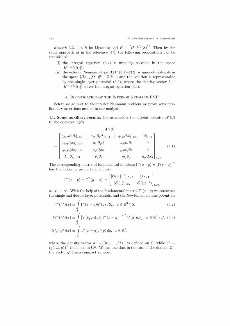
4.1. Some auxiliary results. Let us consider the adjoint operator A∗(∂)to the operator A(∂)

A∗(∂) :=

:=

[ckjrl∂j∂l]3×3 [−ejkl∂j∂l]3×1 [−qjkl∂j∂l]3×1 [0]3×1

[elrj∂j∂l]1×3 κjl∂j∂l ajl∂j∂l 0

[qlrj∂j∂l]1×3 ajl∂j∂l µjl∂j∂l 0

[λrj∂j ]1×3 pj∂j mj∂j ηjl∂j∂l

6×6

. (4.1)

The corresponding matrix of fundamental solutions Γ∗(x−y) = [Γ(y−x)]>

has the following property at infinity

Γ∗(x− y) = Γ>(y − x) :=

[[O(|x|−1)]5×5 [0]5×1

[O(1)]1×5 O(|x|−1)

]

6×6

as |x| → ∞. With the help of the fundamental matrix Γ∗(x−y) we constructthe single and double layer potentials, and the Newtonian volume potentials

V ∗(h∗)(x) ≡∫

S

Γ∗(x− y)h∗(y) dSy, x ∈ R3 \ S, (4.2)

W ∗(h∗)(x) ≡∫

S

[T (∂y, n(y))[Γ∗(x− y)]>]>

h∗(y) dSy, x ∈ R3 \ S, (4.3)

N∗Ω±(g∗)(x) ≡

∫

Ω±

Γ∗(x− y)g∗(y) dy, x ∈ R3,

where the density vector h∗ = (h∗1, . . . , h∗6)> is defined on S, while g∗ =

(g∗1 , ..., g∗6)> is defined in Ω±. We assume that in the case of the domain Ω−

the vector g∗ has a compact support.


It can be shown that the layer potentials V ∗ and W ∗ possess exactly thesame mapping properties and jump relations as the potentials V and W(see Theorems 2.5–2.8). In particular,

V ∗(h∗)+ = V ∗(h∗)− = H∗h∗,W ∗(h∗)± = ± 2−1 h∗ +K∗h∗, (4.4)

PV ∗(h∗)± = ∓ 2−1 h∗ +N ∗h∗, (4.5)

where H∗ is a weakly singular integral operator, while K∗ and N ∗ are sin-gular integral operators,

H∗h∗(x) :=∫

S

Γ∗(x− y)h∗(y) dSy,

K∗h∗(x) :=∫

S

[T (∂y, n(y))[Γ∗(x− y)]>]>

h∗(y) dSy,

N ∗h∗(x) :=∫

S

[P(∂x, n(x))Γ∗(x− y)]h∗(y) dSy.

(4.6)

Now we introduce a special class of vector functions which is a counterpartof the class Z(Ω−).

Definition 4.1. We say that a continuous vector function U∗ =(u∗, ϕ∗, ψ∗, ϑ∗)> has the property Z∗(Ω−) in the domain Ω−, if the fol-lowing conditions are satisfied

U∗(x) =(u∗(x), ϕ∗(x), ψ∗(x)

)> = O(|x|−1) as |x| → ∞,

ϑ∗(x) = O(1) as |x| → ∞,

limR→∞

14πR2

∫

ΣR

ϑ∗(x) dΣR = 0,

where ΣR is a sphere centered at the origin and radius R.

As in the case of usual layer potentials here we have the following

Theorem 4.2. The generalized single and double layer potentials, de-fined by (4.2) and (4.3), solve the homogeneous differential equationA∗(∂)U∗ = 0 in R3 \ S and possess the property Z∗(Ω−).

For an arbitrary regular solution to the equation A∗(∂)U∗(x) = 0 in Ω+

one can derive the following integral representation formula

W ∗(U∗+)(x)− V ∗(PU∗+)(x) =

U∗(x) for x ∈ Ω+,

0 for x ∈ Ω−.(4.7)


Similar representation formula holds also for an arbitrary regular solution tothe equation A∗(∂)U∗(x) = 0 in Ω− which possesses the property Z∗(Ω−):

−W ∗(U∗−S)(x) + V ∗(PU∗−S

)(x) =

U∗(x), x ∈ Ω−,

0, x ∈ Ω+.(4.8)

To derive this representation we denote Ω−R :=B(0, R)\Ω+, where B(0, R)is a ball centered at the origin and radius R. Then in view of (4.7) we have

U∗(x) = −W ∗S

(U∗−S)(x) + V ∗

S

(PU∗−S)(x) + Φ∗R(x), x ∈ Ω−R, (4.9)

0 = −W ∗S

(U∗−S)(x) + V ∗

S

(PU∗−S)(x) + Φ∗R(x), x ∈ Ω+, (4.10)

whereΦ∗R(x) := W ∗

ΣR

(U∗)(x)− V ∗

ΣR

(PU∗)(x). (4.11)Here V ∗

M and W ∗M denote the single and double layer potential operators

with integration surface M. Evidently

A∗(∂)Φ∗R(x) = 0, |x| < R. (4.12)

In turn, from (4.9) and (4.10) we get

Φ∗R(x) = U∗(x) + W ∗S

(U∗−S)(x)− V ∗

S

(PU∗−S)(x), x ∈ Ω−R,

Φ∗R(x) = W ∗S

(U∗−S)(x)− V ∗

S

(PU∗−S)(x), x ∈ Ω+,

(4.13)

whence the equality Φ∗R1(x) = Φ∗R2

(x) follows for |x| < R1 < R2. Weassume that R1 and R2 are sufficiently large numbers. Therefore, for anarbitrary fixed point x ∈ R3 the following limit exists

Φ∗(x) := limR→∞

Φ∗R(x) =

=

U∗(x) + W ∗

S

(U∗−S)(x)− V ∗

S

(PU∗−S)(x), x ∈ Ω−,

W ∗S

(U∗−S)(x)− V ∗

S

(PU∗−S)(x), x ∈ Ω+,

(4.14)

and A∗(∂)Φ∗(x) = 0 for all x ∈ Ω+ ∪Ω−. On the other hand, for arbitraryfixed point x ∈ R3 and a number R1, such that |x| < R1 and Ω+ ⊂ B(0, R1),from (4.13) we have

Φ∗(x) = limR→∞

Φ∗R(x) = Φ∗R1(x).

Now from (4.11)–(4.12) we deduce

A∗(∂)Φ∗(x) = 0 ∀x ∈ R3. (4.15)

Since U∗, W ∗, V ∗ ∈ Z∗(Ω−) we conclude from (4.14) that Φ∗(x) ∈ Z∗(R3).In particular, we have

limR→∞

14πR2

∫

ΣR

Φ∗(x) dΣR = 0. (4.16)

Our goal is to show that

Φ∗(x) = 0 ∀x ∈ R3.


Applying the generalized Fourier transform to equation (4.15) we get

A∗(−iξ)Φ∗(ξ) = 0, ξ ∈ R3,

where Φ∗(ξ) is the Fourier transform of Φ∗. Taking into account thatdetA∗(−iξ) 6= 0 for all ξ ∈ R3 \ 0, we conclude that the support ofthe generalized functional Φ∗(ξ) is the origin and consequently

Φ∗(ξ) =∑

|α|≤M

cαδ(α)(ξ),

where α is a multi-index, cα are arbitrary constant vectors and M is somenonnegative integer. Then it follows that Φ∗(x) is polynomial in x and dueto the inclusion Φ∗ ∈ Z∗(Ω−), Φ∗(x) is bounded at infinity, i.e., Φ∗(x) =const in R3. Therefore (4.16) implies that Φ∗(x) vanishes identically in R3.This proves that the formula (4.8) holds.

Theorem 4.3. Let S ∈ C2,κ and h ∈ [C1,κ′(S)

]6 with 0 < κ′ < κ ≤ 1.Then for the double layer potential W ∗ defined by (4.3) there holds thefollowing formula (generalized Lyapunov–Tauber relation)

PW ∗(h)+ =

PW ∗(h)− on S, (4.17)

where the operator P is given by (2.18).

For h ∈ [H122 (S)]6 the relation (4.17) also holds in the space [H− 1

22 (S)]6.

Proof. Since h ∈ [C1,κ′(S)

]6, evidently U∗ := W ∗(h) ∈ [C1,κ′(Ω±)]6.It is clear that the vector U∗ is a solution of the homogeneous equationA∗(∂)U∗(x) = 0 in Ω+ ∪ Ω−, where the operator A∗(∂) is defined by (4.1).With the help of (4.7) and (4.8), for the vector function U∗ we derive thefollowing representation formula

U∗(x) = W ∗([U∗]S)(x)− V ∗([PU∗]S)(x), x ∈ Ω+ ∪ Ω−, (4.18)

where

[U∗]S ≡ U∗+ − U∗− and [PU∗]S ≡ PU∗+ − PU∗− on S.

In view of the equality U∗ = W ∗(h), from (4.18) we get

W ∗(h)(x) = W ∗([W ∗(h)]S)(x)− V ∗([PW ∗(h)]S)(x), x ∈ Ω+ ∪ Ω−.

Using the jump relation (4.4), we find

[U∗]S = [W ∗(h)]S = W ∗(h)+ − W ∗(h)− = h.

Therefore

W ∗(h)(x) = W ∗(h)(x)− V ∗([PW ∗(h)]S)(x), x ∈ Ω+ ∪ Ω−,

i.e., V ∗(Φ∗)(x) = 0 in Ω+ ∪Ω−, where Φ∗ := [PW ∗(h)]S . With the help ofthe jump relation (4.5) finally we arrive at the equation

0 = PV ∗(Φ∗)− − PV ∗(Φ∗)+ =

= Φ∗ = [PW ∗(h)]S = PW ∗(h)+ − PW ∗(h)−


on S, which completes the proof for the regular case.The second part of the theorem can be proved by standard limiting pro-

cedure. ¤

Let us consider the interior and exterior homogeneous Dirichlet BVPsfor the adjoint operator A∗(∂)

A∗(∂)U∗ = 0 in Ω±, (4.19)

U∗± = 0 on S. (4.20)

In the case of the interior problem, we assume that either U∗ is a regularvector of the class [C1,κ′(Ω+)]6 or U∗ ∈ [W 1

2 (Ω+)]6, while in the case ofthe exterior problem, we assume that either U∗ ∈ [C1,κ′(Ω−)]6 ∩Z∗(Ω−) orU∗ ∈ [W 1

2,loc(Ω−)]6 ∩ Z∗(Ω−).

Theorem 4.4. The interior and exterior homogeneous Dirichlet typeBVPs (4.19)–(4.20) have only the trivial solution in the appropriate spaces.

Proof. First we treat the exterior Dirichlet problem. In view of the structureof the operator A∗(∂), it is easy to see that we can consider separately theBVP for the vector function U∗ = (u∗, ϕ∗, ψ∗)>, constructed by the firstfive components of the solution vector U∗,

A∗(∂)U∗(x) = 0, x ∈ Ω−, (4.21)

U∗(x)− = 0, x ∈ S, (4.22)

where A∗(∂) is the 5× 5 matrix differential operator, obtained from A∗(∂)by deleting the sixth column and the sixth row,

A∗(∂) :=

[ckjrl∂j∂l]3×3 [−ejkl∂j∂l]3×1 [−qjkl∂j∂l]3×1

[elrj∂j∂l]1×3 κjl∂j∂l ajl∂j∂l

[qlrj∂j∂l]1×3 ajl∂j∂l µjl∂j∂l

5×5

. (4.23)

With the help of Green’s identity in Ω−R = B(0, R)\Ω+, we have∫

Ω−R

[U∗ · A∗(∂)U∗ + E(U∗, U∗)

]dx =

= −∫

S

U∗− · P (∂, n)U∗− dS +∫

ΣR

U∗ · P (∂, n)U∗ dΣR, (4.24)

where

P(∂, n) :=

[crjklnj∂l]3×3 [−elrjnj∂l]3×1 [−qlrjnj∂l]3×1

[ejklnj∂l]1×3 κjlnj∂l ajlnj∂l

[qjklnj∂l]1×3 ajlnj∂l µjlnj∂l

5×5

, (4.25)

and


E(U∗, U∗) = crjkl∂lu∗k∂ju

∗r + κjl∂lϕ

∗∂jϕ∗+

+ ajl(∂lϕ∗∂jψ

∗ + ∂jψ∗∂lϕ

∗) + µjl∂lψ∗∂jψ

∗. (4.26)

Due to the fact that U∗ has the property Z∗(Ω−), it follows that U∗ =O(|x|−1) and ∂jU

∗ = O(|x|−2) as |x| → ∞, j = 1, 2, 3. Therefore,∣∣∣∣∫

ΣR

U∗ · P (∂, n)U∗ dΣR

∣∣∣∣ ≤

≤∫

ΣR

C

R3dΣR =

C

R34πR2 =

4πC

R→ 0 as R →∞. (4.27)

Taking into account that E(U∗, U∗) ≥ 0, applying the relations (4.21),(4.22), and (4.27), from (4.24) we conclude that E(U∗, U∗) = 0. Hencein view of (2.10)-(2.11) it follows that U∗ = (a×x+b, b4, b5), where a and bare arbitrary constant vectors, and b4 and b5 are arbitrary scalar constants.Here the symbol × denotes the cross product operation. Due to the bound-ary condition (4.22) we get then a = b = 0 and b4 = b5 = 0, from which wederive that U∗ = 0. Since U∗ vanishes in Ω−, from (4.19)–(4.20) we arriveat the following boundary-value problem for ϑ∗,

ηkj∂k∂jϑ∗ = 0 in Ω−,

ϑ∗− = 0 on S.(4.28)

From boundedness of ϑ∗ at infinity and from (4.28) one can derive thatϑ∗(x) = C + O(|x|−1), where C is an arbitrary constant. In view of U∗ ∈Z∗(Ω−) we have C = 0 and ϑ∗(x) = O(|x|−1), ∂jϑ

∗(x) = O(|x|−2), j =1, 2, 3. Therefore we can apply Green’s formula

∫

Ω−R

[ϑ∗ ηkj∂k∂jϑ

∗ + ηkj∂kϑ∗ ∂jϑ∗]dx =

= −∫

S

ϑ∗−ηkjnk∂jϑ

∗− dS +∫

ΣR

ϑ∗ ηkjnk∂jϑ∗ dΣR.

Passing to the limit as R →∞, we get∫

Ω−

ηkj∂kϑ∗∂jϑ∗ dx = 0.

Using the fact that the matrix [ηkj ]3×3 is positive definite, we conclude thatϑ∗ = C1 = const and since ϑ∗(x) = O(|x|−1) as |x| → ∞, finally we getthat ϑ∗ = 0 in Ω−. Thus U∗ = 0 in Ω− which completes the proof for theexterior problem.

The interior problem can be treated quite similarly. ¤


4.2. Investigation of the interior Neumann BVP. First let us treatthe uniqueness question. To this end we consider the homogeneous interiorNeumann-type BVP

A(∂)U(x) = 0, x ∈ Ω+, (4.29)T (∂, n)U(x)

+ = 0, x ∈ S = ∂Ω+. (4.30)

It can be shown that a general solution to the problem (4.29)-(4.30) can berepresented in the form (for details see [20])

U =9∑

k=1

CkU (k) in Ω+, (4.31)

where Ck are arbitrary scalar constants and U (k)9k=1 is the basis in thespace of solution vectors of the homogeneous problem (4.29)–(4.30). Theycan be constructed explicitly and read as

U (k) =(V (k), 0

)>, k = 1, 8, U (9) =

(V (9), 1

)>, (4.32)

where U (k) = (u(k), ϕ(k), ψ(k), ϑ(k))>, V (k) = (u(k), ϕ(k), ψ(k))>,

V (1) = (0,−x3, x2, 0, 0)>, V (2) = (x3, 0,−x1, 0, 0)>,

V (3) = (−x2, x1, 0, 0, 0)>, V (4) = (1, 0, 0, 0, 0)>,

V (5) = (0, 1, 0, 0, 0)>, V (6) = (0, 0, 1, 0, 0)>,

V (7) = (0, 0, 0, 1, 0)>, V (8) = (0, 0, 0, 0, 1)>,

and V (9) is defined as

V (9) = (u(9), ϕ(9), ψ(9))>, u(9)k = bkqxq, k = 1, 2, 3,

ϕ(9) = cqxq, ψ(9) = dqxq,

with the twelve coefficients bkq = bqk, cq and dq, k, q = 1, 2, 3, defined bythe uniquely solvable linear algebraic system of equations

crjklbkl + elrjcl + qlrjdl = λrj , r, j = 1, 2, 3,

−ejklbkl + κjlcl + ajldl = pj , j = 1, 2, 3,

−qjklbkl + ajlcl + µjldl = mj , j = 1, 2, 3.

From (4.31) it follows that U can be alternatively written as

U = (V , 0)> + b6(V (9), 1)>

with V = (a × x + b, b4, b5)>, where a = (a1, a2, a3)> and b = (b1, b2, b3)>

are arbitrary constant vectors and b4, b5, b6 are arbitrary scalar constants.Now, we start the investigation of the non-homogeneous interior Neu-

mann-type BVP

A(∂)U(x) = 0, x ∈ Ω+, (4.33)T (∂, n)U(x)

+ = F (x), x ∈ S, (4.34)


where U ∈ [C1,κ′(Ω+)]6∩[C2(Ω+)]6 is a sought for vector and F ∈ [C0,κ′(S)]6

is a given vector-function. It is clear that if the problem (4.33)–(4.34) issolvable, then a solution is defined within a summand vector of type (4.31).

We look for a solution to the problem (4.33)–(4.34) in the form of thesingle layer potential,

U(x) = V (h)(x), x ∈ Ω+, (4.35)

where h = (h1, . . . , h6)> ∈ [C0,κ′(S)]6 is an unknown density. From theboundary condition (4.34) and by virtue of the jump relation (2.21) (seeTheorem 2.5) we get the following integral equation for the density vector h

[−2−1I6 +K]h = F on S, (4.36)

whereK is a singular integral operator defined by (2.24). Note that−2−1I6+K is a singular integral operator of normal type with index zero (cf. [23]).Now we investigate the null space Ker(−2−1I6+K). To this end, we considerthe homogeneous equation

[−2−1I6 +K]h = 0 on S (4.37)

and assume that a vector h(0) is a solution to (4.37), i.e., h(0)∈Ker(−2−1I6+K). Since h(0) ∈ [C0,κ′(S)]6, it is evident that the corresponding single layerpotential U0(x) = V (h(0))(x) belongs to the space of regular vector func-tions and solves the homogeneous equation A(∂)U0(x) = 0 in Ω+. Moreover,T (∂, n)U0(x)+ = −2−1h(0) + Kh(0) = 0 on S due to (4.37), i.e., U0(x)solves the homogeneous interior Neumann problem. Therefore, in accor-

dance to the above results, we can write U0(x) =9∑

k=1

CkU (k)(x) in Ω+,

where Ck, k = 1, 9, are some constants, and the vectors U (k)(x) are definedby (4.32). Hence we have

V (h(0))(x) =9∑

k=1

CkU (k)(x), x ∈ Ω+.

If we take into account the jump relation (2.20), we derive that

V (h(0))(x)

+ ≡ H(h(0))(x) =9∑

k=1

CkU (k)(x), x ∈ S. (4.38)

The operators

H : [H− 12 (S)]6 → [H

12 (S)]6,

: [C0,κ′(S)]6 → [C1,κ′(S)]6

are invertible ([19], [23]). Therefore from (4.38) we obtain

h(0) =9∑

k=1

Ckh(k)(x), x ∈ S,


with

h(k) := H−1(U (k)), k = 1, 9. (4.39)

Further we show that the system of vectors h(k)9k=1 is linearly indepen-dent. Let us assume the opposite. Then there exist constants ck, k = 1, 9,

such that9∑

k=1

|ck| 6= 0 and the following equation

9∑

k=1

ckh(k) = 0 on S

holds, i.e.,9∑

k=1

ckH−1(U (k)) = 0 on S. Hence we get

H−1( 9∑

k=1

ckU (k))

= 0 on S,

and, consequently,9∑

k=1

ckU (k)(x) = 0, x ∈ S. (4.40)

Now consider the vector

U∗(x) ≡9∑

k=1

ckU (k)(x), x ∈ Ω+.

Since the vectors U (k) are solutions of the homogeneous equation (4.33), inview of (4.40) we have

A(∂)U∗(x) = 0, x ∈ Ω+,

U∗(x)+ = 9∑

k=1

ckU (k)(x)+

= 0, x ∈ S.

That is, U∗ is a solution of the homogeneous interior Dirichlet problem andin accordance with the uniqueness theorem for the interior Dirichlet BVPwe conclude U∗(x) = 0 in Ω+, i.e.,

9∑

k=1

ckU (k)(x) = 0, x ∈ Ω+.

This contradicts to linear independence of the system U (k)9k=1. Thus, thesystem of the vectors h(k)9k=1 is linearly independent which implies that

dim Ker(−2−1I6 +K) ≥ 9.

Next we show thatdim Ker(−2−1I6 +K) ≤ 9.

Let the equation (−2−1I6+K)h = 0 have a solution h(10) which is not repre-sentable in the form of a linear combination of the system h(k)9k=1. Then


the system h(k)10k=1 is linearly independent. It is easy to show that thesystem of the corresponding single layer potentials V (k)(x) := V (h(k))(x),k = 1, 10, x ∈ Ω+, is linearly independent as well. Indeed, let us assumethe opposite. Then there are constants ak, such that

U(x) :=10∑

k=1

akV (k)(x) = 0, x ∈ Ω+, (4.41)

with10∑

k=1

|ak| 6= 0. From (4.41) we then derive that U(x)+ = 0, x ∈ S.

Therefore,

U+ =10∑

k=1

akV (k)+ =10∑

k=1

akH(h(k)) = H( 10∑

k=1

akh(k))

= 0 on S.

Whence, due to the invertibility of the operator H, we get10∑

k=1

akh(k) = 0 on S.

which contradicts to the linear independence of the system h(k)10k=1.Thus the system V (h(k))(x)10k=1 is linearly independent.On the other hand, we have

A(∂)V (k)(x) = 0, x ∈ Ω+,T V (k)

+ = (−2−1I6 +K)h(k) = 0, x ∈ S,

since h(k), k = 1, 10, are solutions to the homogeneous equation (4.37).Therefore, the vectors V (k), k = 1, 10, are solutions to the homogeneousinterior Neumann-type BVP and they can be expressed by linear combi-nations of the vectors U (j), j = 1, 9, defined in (4.32). Whence it fol-lows that the system V (k)10k=1 is linearly dependent and so is the systemh(k)10k=1 for an arbitrary solution h(10) of the equation (4.37). Conse-quently, dim Ker(−2−1I6 +K) ≤ 9 implying that dim Ker(−2−1I6 +K) = 9.We can consider the system h(1), . . . , h(9) defined in (4.39) as basis vectorsof the null space of the operator −2−1I6 +K. If h0 is a particular solutionto the nonhomogeneous integral equation (4.36), then a general solution ofthe same equation is represented as

h = h0 +9∑

k=1

ckh(k),

where ck are arbitrary constants.For our further analysis we need also to study the homogeneous interior

Neumann-type BVP for the adjoint operator A∗(∂), which reads as follows

A∗(∂)U∗ = 0 in Ω+, (4.42)

PU∗+ = 0 on S = ∂Ω+; (4.43)


here the adjoint operator A∗(∂) and the boundary operator P are definedby (4.1) and (2.18) respectively.

Note that in the case of the problem (4.42)–(4.43) we get also two sepa-rated problems:

a) For the vector function U∗ ≡ (u∗, ϕ∗, ψ∗)>,

A∗(∂)U∗ = 0 in Ω+, (4.44)PU∗+ = 0 on S, (4.45)

where A∗ and P are defined by (4.23) and (4.25) respectively, andb) For the function U∗

6 ≡ ϑ∗

λrj∂ju∗r + pj∂jϕ

∗ + mj∂jψ∗ + ηjl∂j∂lϑ

∗ = 0 in Ω+, (4.46)

ηjlnj∂lϑ∗ = 0 on S. (4.47)

For a regular solution vector U∗ of the problem (4.44)–(4.45) we can writethe following Green’s identity∫

Ω+

[U∗ · A∗(∂)U∗ + E(U∗, U∗)

]dx =

∫

∂Ω+

U∗+ · P(∂, n)U∗+dS, (4.48)

where E is given by (4.26). If we take into account the conditions (4.44)–(4.45), from (4.48) we get ∫

Ω+

E(U∗, U∗) dx = 0.

Hence we have that ∂jϕ∗ = 0, ∂jψ

∗ = 0, j = 1, 2, 3, and ∂lu∗k + ∂ju

∗r = 0

in Ω+. Therefore, u∗(x) = a× x + b is a rigid displacement vector, ϕ∗ = b4

and ψ∗ = b5 are arbitrary constants in Ω+. It is evident that

λrj∂ju∗r =

12

λrj(∂ju∗r + ∂ru

∗j ) = 0

and pj∂jϕ∗ = mj∂jψ

∗ = 0. Then from (4.46)–(4.47) we get the followingBVP for the scalar function ϑ∗,

ηjl∂j∂lϑ∗ = 0 in Ω+,

ηjlnj∂lϑ∗ = 0 on S.

Using the following Green’s identity∫

Ω+

ηjl∂j∂lϑ∗ ϑ∗ dx = −

∫

Ω+

ηjl∂lϑ∗ ∂jϑ

∗ dx +∫

∂Ω+

ηjlnj∂lϑ∗+∂jϑ

∗+ dS,

we find ∫

Ω+

ηjl∂lϑ∗ ∂jϑ

∗ dx = 0,

and by the positive definiteness of the matrix [ηjl]3×3 we get ∂jϑ∗ = 0,

j = 1, 3, in Ω+, i.e., ϑ∗ = b6 = const in Ω+. Consequently, a general


solution U∗ = (u∗, ϕ∗, ψ∗, ϑ∗)> of the adjoint homogeneous BVP (4.42)–(4.43) can be represented as

U∗(x) =9∑

k=1

CkU∗(k)(x), x ∈ Ω+,

where Ck are arbitrary scalar constants, while

U∗(1) = (0,−x3, x2, 0, 0, 0)>, U∗(2) = (x3, 0,−x1, 0, 0, 0)>,

U∗(3) = (−x2, x1, 0, 0, 0, 0)>, U∗(4) = (1, 0, 0, 0, 0, 0)>,

U∗(5) = (0, 1, 0, 0, 0, 0)>, U∗(6) = (0, 0, 1, 0, 0, 0)>,

U∗(7) = (0, 0, 0, 1, 0, 0)>, U∗(8) = (0, 0, 0, 0, 1, 0)>,

U∗(9) = (0, 0, 0, 0, 0, 1)>.

(4.49)

As we see, U∗(k) = U (k), k = 1, 8, where U (k), k = 1, 8, is given in (4.32).One can easily check that the system U∗(k)9k=1 is linearly independent.As a result we get the following

Proposition 4.5. The space of solutions of the adjoint homogeneous BVP(4.42)–(4.43) is nine dimensional and an arbitrary solution can be repre-sented as a linear combination of the vectors

U∗(k)

9

k=1, i.e., the system

U∗(k)9k=1 is a basis in the space of solutions to the homogeneous BVP(4.42)–(4.43).

Now, we return to equation (4.36) and consider the corresponding homo-geneous adjoint equation

(−2−1I6 +K∗)h∗ = 0 on S,

where K∗ is the adjoint operator to K defined by the duality relation,

(Kh, h∗)L2(S) = (h,K∗h∗)L2(S), ∀h, h∗ ∈ [L2(S)]6.

It is easy to show that the operator K∗ is the same as the operator givenby (4.6). In what follows we prove that dim Ker

(− 12 I6 +K∗) = 9.

Indeed, in accordance with Proposition 4.5 we have that A∗(∂)U∗(k) = 0in Ω+ and PU∗(k)+ = 0 on S. Therefore from (4.7) we have

U∗(k)(x) = W ∗(U∗(k)+)(x), x ∈ Ω+. (4.50)

By the jump relations (4.4) we get

h∗(k) = 2−1 h∗(k) +K∗h∗(k) on S,

whereh∗(k) := U∗(k)+, k = 1, 9. (4.51)

Whence it follows that(− 2−1 I6 +K∗)h∗(k) = 0, k = 1, 9.


By Theorem 4.4 and the relations (4.50) and (4.51) we conclude that thesystem

h∗(k)

9

k=1is linearly independent, and therefore

dimKer(− 2−1 I6 +K∗) ≥ 9.

Now, let h∗(0) ∈ Ker(− 2−1 I6 + K∗), i.e.,

(− 2−1 I6 + K∗)h∗(0) = 0. Thecorresponding double layer potential U∗

0 (x) := W ∗(h∗(0))(x) is a solution tothe homogeneous equation A∗(∂)U∗

0 = 0 in Ω+. Moreover, W ∗(h∗(0))− =−2−1 h∗(0) + K∗h∗(0) = 0 on S. Consequently, U∗

0 is a solution of thehomogeneous exterior Dirichlet BVP possessing the property Z∗(Ω−). Withthe help of the uniqueness Theorem 4.4 we conclude that W ∗(h∗(0)) = 0 inΩ−. Further,

PW ∗(h∗(0))+ = PW ∗(h∗(0))− = 0 due to Theorem 4.3,

and for the vector function U∗0 we arrive at the following BVP,

A∗(∂)U∗0 = 0 in Ω+,

PU∗0

+ = 0 on S.

Using Proposition 4.5 we can write

U∗0 (x) = W ∗(h∗(0))(x) =

9∑

k=1

ckU∗(k)(x), x ∈ Ω+,

where ck are some constants. The jump relation for the double layer poten-tial then gives

W ∗(h∗(0))(x)

+ − W ∗(h∗(0))(x)

−

= h∗(0)(x) =9∑

k=1

ck

U∗(k)(x)

+ =9∑

k=1

ckh∗(k)(x), x ∈ S,

which implies that the systemh∗(k)

9

k=1represents a basis of the null space

Ker(− 2−1 I6 +K∗). Whence it follows that dim Ker

(− 2−1 I6 +K∗) = 9.Now we can formulate the following basic existence theorem for the in-

tegral equation (4.36) and the interior Neumann-type BVP.

Theorem 4.6. Let m ≥ 0 be a nonnegative integer and 0 < κ′ < κ ≤ 1.Further, let S ∈ Cm+1,κ and F ∈ [Cm,κ′(S)]6. The necessary and sufficientconditions for the integral equation (4.36) and the interior Neumann-typeBVP (4.33)–(4.34) to be solvable read as

∫

S

F (x) · h∗(k)(x) dS = 0, k = 1, 9, (4.52)

where the system h∗(k)9k=1 is defined explicitly by (4.51) and (4.49).If these conditions are satisfied, then a solution vector to the interior

Neumann-type BVP is representable by the single layer potential (4.35),where the density vector h ∈ [Cm,κ′(S)]6 is defined by the integral equa-tion (4.36).


A solution vector function U ∈ [Cm+1,κ′(Ω+)]6 is defined modulo a linearcombination of the vector functions U (k)9k=1 given by (4.32).

Remark 4.7. Similar to the exterior problem, if S is a Lipschitz surface,F ∈ [

H−1/2(S)]6

, and the conditions (4.52) is fulfilled, then

(i) the integral equation (4.36) is solvable in the space[H−1/2(S)

]6;(ii) the interior Neumann-type BVP (4.33)-(4.34) is solvable in the

space[H1

2 (Ω+)]6 and solutions are representable by the single layer

potential (4.35), where the density vector h ∈ [H−1/2(S)

]6 solvesthe integral equation (4.36);

(iii) A solution U ∈ [H1

2 (Ω+)]6 to the interior Neumann-type BVP

(4.33)-(4.34) is defined modulo a linear combination of the vectorfunctions

U (k)

9

k=1given by (4.32).

Acknowledgements

This research was supported partly by the Georgian Technical UniversityGrant - GTU-2011/4.

References

1. M. S. Agranovich, Elliptic singular integro-differential operators. (Russian) Usp.Mat. Nauk 20 (1965), No. 5(125), 3–120.

2. M. Avellaneda and G. Harshe, Magnetoelectric effect in piezoelectric / magne-tostrictive multilayer (2-2) composites. J. Intelligent Mater. Syst. Struct. 5 (1994),501–513.

3. Y. Benveniste, Magnetoelectric effect in fibrous composites with piezoelectric andpiezomagnetic phases. Phys. Rev. B 51 (1995), 424–427.

4. W. F. Jr. Brown, Magnetoelastic interaction, Springer, New York, 1966.5. T. Buchukuri, O. Chkadua, D. Natroshvili, and A.-M. Sandig, Solvability and

regularity results to boundary-transmission problems for metallic and piezoelectricelastic materials. Math. Nachr. 282 (2009), No. 8, 1079–1110.

6. T. Buchukuri, O. Chkadua, D. Natroshvili, and A.-M. Sandig, Interaction prob-lems of metallic and piezoelectric materials with regard to thermal stresses. Mem.Differential Equations Math. Phys. 45 (2008), 7–74.

7. T. Buchukuri, O. Chkadua, and D. Natroshvili, Mixed boundary value prob-lems of thermopiezoelectricity for solids with interior cracks, Integral Equations andOperator Theory. 64 (2009), No. 4, 495–537.

8. M. Costabel, Boundary integral operators on Lipschitz domains: elementary results.SIAM J. Math. Anal. 19 (1988), No. 3, 613–626.

9. R. Duduchava, The Green formula and layer potentials, Integral Equations andOperator Theory. 41 (2001), No. 2, 127–178.

10. R. Duduchava, D. Natroshvili, and E. Shargorodsky, Boundary value problemsof the mathematical theory of cracks. Tbiliss. Gos. Univ. Inst. Prikl. Mat. Trudy 39(1990), 68–84.

11. R. Duduchava, D. Natroshvili, and E. Shargorodsky, Basic boundary valueproblems of thermoelasticity for anisotropic bodies with cuts. I. Georgian Math. J.2 (1995), No. 2, 123–140; II. Georgian Math. J. 2 (1995), No. 3, 259–276.

12. G. C. Hsiao and W. L. Wendland, Boundary integral equations. Applied Mathe-matical Sciences, 164. Springer-Verlag, Berlin, 2008.


13. L. Jentsch and D. Natroshvili, Three-dimensional mathematical problems of ther-moelasticity of anisotropic bodies. I. Mem. Differential Equations Math. Phys. 17(1999), 7–126.

14. L. Jentsch and D. Natroshvili, Three-dimensional mathematical problems of ther-moelasticity of anisotropic bodies. II. Mem. Differential Equations Math. Phys. 18(1999), 1–50.

15. V. D. Kupradze, T. G. Gegelia, M. O. Basheleishvili, and T. V. Burchuladze,Three-dimensional problems of the mathematical theory of elasticity and thermoe-lasticity. Translated from the second Russian edition. Edited by V. D. Kupradze.North-Holland Series in Applied Mathematics and Mechanics, 25. North-HollandPublishing Co., Amsterdam-New York, 1979.

16. J. Y. Li, Uniqueness and reciprocity theorems for linear thermo-electro-magneto-elasticity. Quart. J. Mech. Appl. Math. 56 (2003), No. 1, 35–43.

17. W. McLean, Strongly elliptic systems and boundary integral equations. CambridgeUniversity Press, Cambridge, 2000.

18. S. G. Mikhlin and S. Prossdorf, Singular integral operators. Translated from theGerman by Albrecht Bottcher and Reinhard Lehmann. Springer-Verlag, Berlin, 1986.

19. M. Mrevlishvili, Investigation of interior and exterior Dirichlet BVPs of thermo-electro-magneto elasticity theory and regularity results. Bull. TICMI (to appear).

20. M. Mrevlishvili, D. Natroshvili, and Z. Tediashvili, Uniqueness theorems forthermo-electro-magneto-elasticity problems. Bull. Greek Math. Soc. 57 (2010), 281–295.

21. C. W. Nan, Magnetoelectric effect in composites of piezoelectric and piezomagneticphases. Phys. Rev. B 50 (1994), 6082–6088.

22. D. Natroshvili, Boundary integral equation method in the steady state oscillationproblems for anisotropic bodies. Math. Methods Appl. Sci. 20 (1997), No. 2, 95–119.

23. D. Natroshvili, Mathematical problems of thermo-electro-magneto-elasticity (toappear).

24. D. Natroshvili, T. Buchukuri, and O. Chkadua, Mathematical modelling andanalysis of interaction problems for piezoelastic composites. Rend. Accad. Naz. Sci.XL Mem. Mat. Appl. (5) 30 (2006), 159–190.

25. D. Natroshvili, O. Chkadua, and E. Shargorodsky, Mixed problems for homo-geneous anisotropic elastic media. (Russian) Tbiliss. Gos. Univ. Inst. Prikl. Mat.Trudy 39 (1990), 133–181.

26. D. G. Natroshvili, A. Ya. Djagmaidze, and M. Zh. Svanadze, Some problemsin the linear theory of elastic mixtures. (Russian) With Georgian and English sum-maries. Tbilis. Gos. Univ., Tbilisi, 1986.

27. W. Nowackiı, Electromagnetic effects in solids. (Russian) Translated from the Polishand with a preface by V. A. Shachnev. Mechanics: Recent Publications in ForeignScience, 37. “Mir”, Moscow, 1986.

28. R. T. Seeley, Singular integrals and boundary value problems. Amer. J. Math. 88(1966), 781–809.

29. H. Triebel, Interpolation theory, function spaces, differential operators. North-Holland Mathematical Library, 18. North-Holland Publishing Co., Amsterdam–NewYork, 1978.

(Received 18.03.2011)

Authors’ address:

Department of Mathematics, Georgian Technical University77, M. Kostava Str., Tbilisi 0175GeorgiaE-mail: m−[email protected], [email protected]

Documents

· Abstract. We investigate the three-dimensional interior and exterior Neumann-type boundary-value problems of statics of the thermo-electro-magneto-elasticity theory