NASA Cs.radw • ,AD-A280 58010M ftmorI No, %#-W3

*ICASEA PHASE EQUATION APPROACH TOBOUNDARY LAYER INSTABILITY THEORY:TOLLMIEN SCHLICHTING WAVES

DTICPhilip Hall $ E T 0

F !:

~ais uass TiC QUALM W~RT8

94-19273Contract NASI-19480 II IiIH 1111I111111lApril IMii

institute for Computer Applications in Science and EngineenngNASA Langley Research CenterAmon, VA 23681-o001

SOperated by Universities Space Research Association

23 089

ICASE Fluid Mechanics

Due to increasing research being conducted at ICASE in the field of fluid mechanics,

future ICASE reports in this area of research will be printed with a green cover. Applied

and numerical mathematics reports will have the familiar blue cover, while computer science

reports will have yellow covers. In all other aspects the reports will remain the same; in

particular, they will continue to be submitted to the appropriate journals or conferences for

formal publication.

Accesion -For

By. ...............................

By............Distribution

AvaiabiSity CoaleDit Avail and ior

1 Special

A PHASE EQUATION APPROACH TO

BOUNDARY LAYER INSTABILITY THEORY:

TOLLMIEN SCHLICHTING WAVES

Philip Hall1

Department of Mathematics

University of Manchester

Manchester M13 9PL, U.K

Abstract

Our concern is with the evolution of large amplitude Tollmien-Schlichting waves in

boundary layer flows. In fact the disturbances we consider are of a comparable size to

the unperturbed state. We shall describe two-dimensional disturbances which are locally

periodic in time and space. This is achieved using a phase equation approach of the type

discussed by Howard and Kopell (1977) in the context of reaction-diffusion equations. We

shall consider both large and 0(1) Reynolds numbers flows though, in order to keep our

asymptotics respectable, our finite Reynolds number calculation will be carried out for the

asymptotic suction flow. Our large Reynolds number analysis, though carried out for Bla-

sius flow, is valid for any steady two-dimensional boundary layer. In both cases the phase

equation approach shows that the wavenumber and frequency will develop shocks or other

discontinuities as the disturbance evolves. As a special case we consider the evolution of con-

stant frequency/wavenumber disturbances and show that their modulational instability is

controlled by Burgers equation at finite Reynolds number and 1y a new integro-differential

evolution equation at large Reynolds numbers. For the large Reynolds number case the

evolution equation points to the development of a spatially localized singularity at a finite

time. The three-dimensional generalizations of the evolution equations is also given for the

case of weak spanwise modulations.

'This research was partially supported by the National Aeronautics and Space Administration under NASA

Contract No. NAS1-19480 while the author was in residence at the Institute for Computer Applications in

Science and Engineering (ICASE), NASA Langley Research Center, Hampton, VA 23665. This work was also

supported by SERC and NSF under contract NSF CTS-9123553

iii

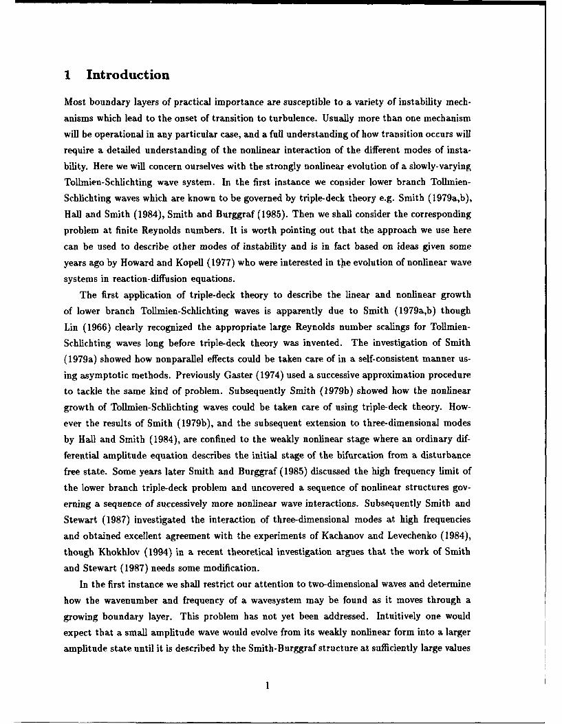
1 Introduction

Most boundary layers of practical importance are susceptible to a variety of instability mech-

anisms which lead to the onset of transition to turbulence. Usually more than one mechanism

will be operational in any particular case, and a full understanding of how transition occurs will

require a detailed understanding of the nonlinear interaction of the different modes of insta-

bility. Here we will concern ourselves with the strongly nonlinear evolution of a slowly-varying

Tollmien-Schlichting wave system. In the first instance we consider lower branch Tollmien-

Schlichting waves which are known to be governed by triple-deck theory e.g. Smith (1979a,b),

Hall and Smith (1984), Smith and Burggraf (1985). Then we shall consider the corresponding

problem at finite Reynolds numbers. It is worth pointing out that the approach we use here

can be used to describe other modes of instability and is in fact based on ideas given some

years ago by Howard and Kopell (1977) who were interested in the evolution of nonlinear wave

systems in reaction-diffusion equations.

The first application of triple-deck theory to describe the linear and nonlinear growth

of lower branch Tollmien-Schlichting waves is apparently due to Smith (1979a,b) though

Lin (1966) clearly recognized the appropriate large Reynolds number scalings for Tollmien-

Schlichting waves long before triple-deck theory was invented. The investigation of Smith

(1979a) showed how nonparallel effects could be taken care of in a self-consistent manner us-

ing asymptotic methods. Previously Gaster (1974) used a successive approximation procedure

to tackle the same kind of problem. Subsequently Smith (1979b) showed how the nonlinear

growth of Tollmien-Schlichting waves could be taken care of using triple-deck theory. How-

ever the results of Smith (1979b), and the subsequent extension to three-dimensional modes

by Hall and Smith (1984), are confined to the weakly nonlinear stage where an ordinary dif-

ferential amplitude equation describes the initial stage of the bifurcation from a disturbance

free state. Some years later Smith and Burggraf (1985) discussed the high frequency limit of

the lower branch triple-deck problem and uncovered a sequence of nonlinear structures gov-

erning a sequence of successively more nonlinear wave interactions. Subsequently Smith and

Stewart (1987) investigated the interaction of three-dimensional modes at high frequencies

and obtained excellent agreement with the experiments of Kachanov and Levechenko (1984),

though Khokhlov (1994) in a recent theoretical investigation argues that the work of Smith

and Stewart (1987) needs some modification.

In the first instance we shall restrict our attention to two-dimensional waves and determine

how the wavenumber and frequency of a wavesystem may be found as it moves through a

growing boundary layer. This problem has not yet been addressed. Intuitively one would

expect that a small amplitude wave would evolve from its weakly nonlinear form into a larger

amplitude state until it is described by the Smith-Burggraf structure at sufficiently large values

of the local frequency of the disturbance. Our calculations show that this is not the case and

indeed show that at high frequencies locally periodic forms of the modes found by Smith and

Burggraf probably do not exist. Certainly it would appear that they do not connect to the

weakly nonlinear state discussed by Smith (1979b).

The asymptotic structure we use is based on the so-called 'phase-equation 'approach used

so successfully to describe large amplitude B~nard convection in large containers by, amongst

others, Kramer, Ben Jacob, Brand and Cross (1982), Cross and Newell (1984), Newell, Passot

and Lega (1993). Using this approach it has been possible to describe the experimentally

observed slowly varying planform of Benard convection. Thus, for example, the dislocation

of convection rolls is now reasonably well understood using the phase equation approach.

Interestingly enough it turns out that the essential ideas of this approach had been elucidated

in the context of traveling wave instabilities several years earlier, see Howard and Kopell (1977)

and indeed the method can be found in Whitham (1974). The evolution of traveling waves in

a Blasius boundary layers is the subject of the first part of this work and not surprisingly the

analysis to be used has similarities with that of the latter authors.

The essential idea behind the phase equation approach may be explained in the following

manner. Suppose there exists some flow which is unstable to a traveling wave disturbance of

wavenumber a and frequency Q. For a fully nonlinear disturbance the frequency R1 will be

a function of a which itself can be thought of as a function of A, a measure of the size of

disturbance. If we let A tend to zero then, for small A, the quantities a and f? will differ from

their linear neutral values by O(A)2 so that finite amplitude disturbances begin as supercritical

bifurcations from the basic state. For 0(1) values of A the quantities a and Q1 are accessible

only by numerical means, see for example Herbert (1977) for details of the computation of a

and fl for Tollmien-Schlichting waves in plane Poisseuille flow or Conlisk, Burggraf and Smith

(1987) for a similar calculation for Tollmien-Schlichting waves in Blasius boundary layers at

large Reynolds numbers. In some cases the frequency of the waves is zero and, the wavenumber

of the disturbances may be sensibly held fixed when the control parameter or disturbance size

is varied, see for example Hall (1988) for a discussion of the fully nonlinear G6rtler problem in

a growing boundary layer. For a traveling wave disturbance in a growing boundary layer we

expect that the wavenumber and frequency of the disturbance should change as it propagates

into locally less or more unstable parts of the flow. The phase equation approach provides

a rational framework for following such an evolution. If the wave has local frequency and

wavenumber which are 0(1) with respect to the variables t and x we introduce slowly varying

variables T and X by writing

T = 6t, X = 6x,

and we now think of a and fl as being functions of X and T. Thus we may introduce the

2

phase function 0(X, T) defined by 0 = O(X, T)/6 with

S= Ox,£ = -OT

and as a consequence the wave system evolves such that

aT + =-. (1.1)

Partial derivatives with respect to x and t must then be replaced using

a a +6a a a219+ a

and if we then equate terms of 0(6)0 we recover the unmodulated equations of motion with a

and 0 playing the role of wavenumber and frequency. Thus the leading order problem using

the phase equation approach is simply the unmodulated case with a and f? being functionally

related in order that the system, with a given disturbance size, has a solution. At next order

(usually 0(6) but in fact 0(6b/l) in triple deck problems) we obtain a linearized inhomogeneous

form of the leading order problem. Due to the invariance of the problem under a translation

in the x direction it is easy to see that the linearized homogeneous form of this system has a

non-trivial solution so that some solvability condition must be satisfied if the inhomogeneous

problem is to have a solution. This solvability condition is satisfied by introducing an expansion

of Q in appropriate powers of 6. The solution of this problem then enables us to write down the

asymptotic form of (1.1) upto the second order. This procedure can be continued in principle

to any order and the coefficients in the expansion of f are found as solvability conditions at

each order. The evolution of a given wave system can then be found by the solution of the

calculated asymptotic approximation to (1.1). We find that (1.1) takes on a particularly simple

form if the wave system has fixed wavenumber and frequency at leading order. We shall in this

paper calculate (1.1) correct upto second order for both wavesystems governed by triple-deck

theory and those satisfying the two-dimensional Navier-Stokes equations. We can show that

at high Reynolds numbers (1.1) may then be reduced to the form

aA . A __t_____8A' + A -8A -0"J ( 9 -- d-,/ (1.2)

This is in effect the evolution equation for a wavepacket of large amplitude Tollmien-

Schlichting waves in a growing boundary layer.

At finite Reynolds numbers the modulation equation corresponding to (1.2) is

A. + AAt = ±AI- . (1.3)

Thus at finite Reynolds numbers Burgers equations controls the slow dynamics of a two-

dimensional wavesystem. We will show that (1.2) and (1.3) can be generalized to allow for a

3

weak spanwise dependence of the modulation and, surprisingly, it turns out that the general-

izations in both cases are achieved by adding a term proportional to A<( to both equations.

Here ( is a slow spanwise variable.

The procedure adopted in the rest of this paper is as follows: In §2 we derive the phase

equation for two-dimensional triple-deck problems. In §3 we describe the numerical work

required to determine the quantities appearing in the equation. In §4 we look at the special

case of almost uniform wavetrains and derive (1.2). In §5 we show how (1.2) can be derived

by a more conventional multiple scale approach directly from the triple-deck equations. The

phase equation approach for a boundary layer at finite Reynolds numbers is then discussed

in §6. The modulation equation (1.3) is derived in that section as a special case for almost

uniform wavetrains. Finally in §7 we draw some conclusions and give the generalized form of

the evolution equations which account for weak spanwise modulations and nonparallel effects.

2 Derivation of the phase equation for 2D triple deck prob-

lems

Our concern is with the structure of fully nonlinear solutions of the triple-deck equations gov-

erning the evolution of two-dimensional Tollhnien-Schlichting waves in incompressible boundary

layers. Following the usual notation, e.g. Smith (1979a), the appropriate differential equations

in scaled form are ou 8V- = 0, (2. 1a)

o au Ottp a' 2uTt + u -ox + V-• T Tz + y-- (2. 1b)

which must be solved subject to

u=v=0, y=0, (2.2a)

u y+ A(x,t), y -• , (2.2b)1 100 9A

=- as ds (2.2c)

The displacement function A and the pressure p depend only on x and t and if we wish to

consider other flows the pressure displacement law (2.2c) must be modified accordingly. Linear

ToUmien-Schlichting waves correspond to perturbing u in the form

u = y + U(y)eiv{zf }, (2.3)

with U small and, from Smith (1979a), the eigenrelation takes the form

Aý (co) = (ia)'/'a 0j Ai(m7 )d?7. (2.4)410

inl

where Ai is the Airy function and fo = (i)2/3 . Solutions of (2.4) with f? complex and a

real show that neutral stability occurs for Q t 2.298, a •_ 1.001, and that Qj is positive for all

frequencies greater than the neutral value. In the high frequency limit it can be shown from

(2.4) that

a = f + O(1- 1/2) (2.5)

The above limit was discussed in detail by Smith and Buggraff (1985) who investigated the

possible nonlinear structures which emerge in that limit. The structures found by Smith and

Burggraf depend crucially on the fact that the right hand side of (2.5) is complex only at orderfl-1/2 so that, even though a wave is never neutral, its growth can be balanced at higher order

by nonlinear effects. Here our interest is with the case a = 0(1),0 = 0(1), but we shall allow

for a slow evolution of the wavesystem as it moves through the boundary layer. The essential

details of our approach are to be found in Howard and Kopell (1977) who were concerned with

slowly varying waves in reaction diffusion systems. As a first step we introduce slow time and

space variables, T and X, by writing

T = bt, (2.6a)

X = bt, (2.6b)

where 6 is a small positive parameter. We shall investigate the evolution of a fully nonlinear

wavelike solution of (2.1)-(2.2), but allow the wavenumber and frequency to be slow function.:

of X and T.

In order to describe such a structure we introduce a phase function 0(z, t) such that the

wavenumber and frequency of the wave are defined by

F , f? =-Tt (2.7)

The wavenumber and frequency must therefore satisfy8a on!S+ n = o, (2.8)

and (2.8) therefore corresponds to the conservation of phase. Now we shall assume, following

Howard and Kopell (1977), that a and fl are functions only of X and T. In that case (2.8)

reduces to 19a 19 0 ( .9T + an (2.9)

and it is then convenient to write to phase variable e = 1-0O(X, T). The x and t derivatives

in (2.1)-(2.2) must then be transformed according to

a- a• +6 , 9(2.10a)

09 a ab (2.1Ob)

5

We seek a locally wavelike solution of (2.1)-(2.2) and impose periodicity in the phase variable

0. It remains now for us to find a small 6 solution of the full triple deck problem (2.1)-(2.2).

At first sight, in view of (2.10), we would expect to develop a solution of that system in terms

of 6. However, it turns out that for 6 << 1 the leading order approximation to (2.1)-(2.2) has

a mean term correction which depends on the slow variable X. This mean flow is reduced to

zero in an outer O(b-1/3) boundary layer. The expansions must therefore proceed in powers

of 51/' and we therefore write

S= 0+ b1 13fli+.., (2.11 a)

u = uo(X,T,E,Y)+6 1/3 u 1(X,T,0,Y) +..., (2.11b)

v = vo(X,T,E,Y)+b 1 / 3v1(X,T,0,Y) + .. , (2.11c)

p = po(X,T,0)+ 6 1 / 3p,(X,T,0)+..., (2.1ld)

A = Ao(X,T,0)+6 1 /3Al(X,T,0)+.... (2.1le)

The leading order problem is then found to be

a U-O + ýO = , (2.12a)

00 OY

0Uo 00Uo 0o 82Uo (2.12b)-- Qo-5- + ,auo-67-) + VO-5-•- = -a- + !L_(2.,b

Uo= v=0, y =0, (2.12c)

uo y + Ao(X, 0, T) y--+ oo, (2.12d)

1 0 aAdib

Po = -- 0 (9- 1) (2.12e)

Hence the leading order problem is obtained from the full two-dimensional problem by restrict-

ing attention to solutions in the form of traveling waves of local wavenumber a and frequency

Ro. This specifies a nonlinear eigenvalue problem

no = Qo(a), (2.13)

which must be determined numerically. At this stage we assume that (2.13) and the corre-

sponding nonlinear eigenfunctions uo, vo, Po and A0 are known. We further note Ao may be

written in the form

Ao = Ao(X,T)+ Ao(O,X,T) (2.14)

where Ao has zero mean with respect to 0. It is necessary to reduce Ao to zero before the main

deck is encountered, therefore an outer boundary layer is required. Before we investigate the

outer boundary layer it is convenient to discuss the next order system in the y = 0(1) region.

The equations to be satisfied are

ý-•6 + -•ui = 0, (2.15a)

6

,0. f Ott 0ol Ol u Opa O 2u1 u- +' + + a •O°-i+u - 0 - + v1 -- +c I-- = 0 -!-6' (2.15b)

subject to

u= V=0, =0, (2.15c)

and

P1 = -a (- -S. (2.15d)

In addition we require a condition involving ul at the edge of the boundary layer. On the basis

of (2.2b) we might expect that, ul --+ A 1, y ---+ oo, is the appropriate condition. However A, is

essentially the displacement function in the main deck and ul is modified in the outer boundary

layer in which the mean flow correction on the slow scale is reduced to zero. Therefore we

must write down the condition

u1 --* D1 , y --* oo, (2.16)

where D1 is to be found in terms of A1 by a consideration of the outer boundary layer. For

large values of y we have u - y so that the thickness of the outer layer is fixed by the balance

0 02

Hence we write

17 = 61/3Y

and now develop an asymptotic solution of (2.1)-(2.2) valid for 77 = 0(1). The solution here is

similar to that in the main deck for two-dimensional triple-deck problems. We write

U = {6-1/3v7 +uM (X,v,,T)"+_.J}+ J{Uo+1131 I" +...I

Here the terms in the first bracket of each expansion correspond to the mean flow. If we

substitute the above expansions into (2.1)-(2.2), and make the ajpropriate changes of variables,

then we find that the function U0 is given by

Uo = A0 + 61/3[it + b113 AouM,, +

where f 1 is to be determined. The functions UM and VM are found to satisfy

0 2 UM OUM

0172 OT- -

19UM OVM+ --- 0

OX O~7

which are to be solved subject to

UM M Ao, vm - O t. 0, Um7 0, ) -- 00.

The solution of the above problem for the mean flow correction is most easily obtained using

a Fourier transform with respect to X. We find that the function UM is such that

UM, 1 1 = 0pU Ids. (2.17)

If we now match the 0(61/3) correction to the wavelike parts of the expansion between the

y = 0(l), y = 0(61/3) regions we obtain

3•Ao fX • .dHl + ds=D,r (1 (-x)1/3

whilst letting 71 -- cc in the definition of U1 gives

H1 = A,. (2.18)

This closes the problem for the order 61/3 problem in the lower layer. Thus in addition to

(2.14), (2.15) and (2.16) we have

3*- X d-

D, = A, + ()O (s- X)/ 3 (2.19)

It should also be pointed out that the condition that the mean flow correction UM goes to zero

at infinity can be relaxed, if required for some A 0 , to the condition that UM tends to a constant

at infinity. This does not alter the condition (2.19). The quantity fl, is now determined as a

solvability condition on the inhomogeneous system specified by (2.15), (2.16) and (2.19). Such

a condition is required because of the translational invariance of the leading order wavesystem

with respect to 0. Therefore a solution of the homogeneous problem is found by settinga

(ul, vi, pi, A1 ) = •-j(uo, vo, p0, Ao). In order to find the appropriate solvability condition it

is convenient to define Z = (pl, v 1, U1, uY)T. We then must determine the condition that the

inhomogeneous system given below has a solution:

Z= BZ+C 8Z-+fF,dyo

0 0 0 0

B0 0 0 0B- =0 0 0 1

0 UoY aUoe VoJ

8

[00 0 0 0

C = 0 0 -41 0 j F0= ]0 0 0 0 0

a 0 auo - no 0 uo9

subject to

UU = V+ = 0, y 00,

A 2 +F(T- X)1/ 3

X - SI"

The system adjoint to the homogeneous form of the above problem is

- =DJ _,T oJ0- -

with0 0 0 0

D 0 0 0 uoy0 00 0

0 0 1 vo

J = (M,N,S,T)T ,

and subject to the conditions

M=T=O, y=O,

s -, 0, y ---+ 00,

M -- M (O), T- Ty- 2 , y- 00 with T 1= - (-)ds.

The condition that the problem for (ul, vi, pi, A 1) has a solution is then found to be,x a_••0 c

d, = 0s ,/6 (2.20)

with3ý f0 Moo(O)podE

K(a) 3() f (2.21)

At this stage we can write down the phase conservation equation correct to order 6 1/3. We

obtain 19a Ono Oa _/l3•+a = - 6/31I! + 0(62/3), (2.22)

dTT Oa x OX

and the expansion procedure given above can in principle be continued to any order. We

postpone a discussion of the implications of (2.22) until we have described the results of the

calculations required to determine a, n•o, Q1.

9

3 The numerical work

The system (2.12) is periodic in 0 so we seek a solution by expanding for example vo in theform

00

Vo E o Wei-, (3.1)00

After eliminating Porn and some linear terms proportional to uo.. from the 0 momentum

equation, the equation to determine von may be written in the form

d 4 Vorn

dy4 - im {auoo - 11} vo0,, = Rill (3.2)

where R,, is a nonlinear function of {Uo,,}, {vo,n}. The equation 'for the mean part of uO is

then written asd2 uoo d (

dy2 •y' (3.3)

where I is a nonlinear function of {uo,,,}, {vom}. We used central differences to evaluate the

derivatives in (3.2), (3.3) and a solution of the resulting nonlinear system was found by iteration

after first restricting m to be less than say M. In our iterative technique the right hand sides

of (3.2) and (3.3) were evaluated at the previous level of iteration and one boundary condition

was replaced by

vo'(oo) = co + ido

where co and do are prescribed real constants. After the iterations converged we then adjusted

a and 0 until the previously ignored boundary condition was satisfied. Note here that , because

the solution of (2.12) is unique only upto a phase shift, the values of a and Q obtained by this

procedure are functions only of {co2 + do}1/2.

The grid size and the value of M were varied until converged results were obtained. In the

following discussion the results presented correspond to M = 32, and 200 grid points in the y

direction with "infinity" at y = 10. In Figures 1 and 2 we show the dependence of a and Qo on

the quantity c0 + do which is a measure of the disturbance size. We see that, as predicted by

Smith (1979b), finite amplitude motion begins as a supercritical bifurcation from Blasius flow.

In Figure 3 we plot Ro as a function of a. The calculations could not be continued beyond the

point F shown on the Figure ; we will return to this point later. We further notice that Ro is a

multiple valued function of a for a range of values of a and that fW•(a) becomes infinite when

a - 1.0145. In Figure 4 we show the shear stress as a function of 0 for a range values of o0 .

The results shown in this picture suggest a reason why Figure 3 cannot be continued beyond

the point F. We see that as the point F is approached the shear stress approaches zero at a

point. In Figure 5 we show how the contribution to the shear stress from the different modes

varies as 120 varies. We see that the the higher modes grow rapidly as F is approached. This

suggests that the shear stress becomes singular as F is approached.

10

Beyond the point F our calculations failed to converge because the procedure used to solve

(3.2)-(3.3) failed to drive the residuals below the tolerance level, 10-12, used throughout our

work. A similar result was found by Conlisk et al (1987) who solved (2.12) by an indirect

method. In their calculation the Tollmien-Sclichting waves were first forced by a wall motion

and then their properties extrapolated as the forcing was reduced to zero. The results of

Conlisk et al (1987) have been plotted in Figure 3 and we see that, on the whole, there is

good agreement with our work when our program produced converged results. Some of the

larger amplitude results by Conlisk et al were obtained by reducing the tolerance level in

their iteration procedure. A similar reduction of the tolerance level in our code enables us to

continue Figure 3 for slightly larger disturbance amplitudes but we do not plot them for the

following reasons. Firstly we found that a reduction of the tolerance level made our results

very sensitive to the grid size. Secondly a reduction of the tolerance level at best only enabled

us to continue our calculation until a was reduced to about 1.018. Furthermore the results of

Figure 4 suggest to us that the curve of Figure 3 terminates at a point close to F where all

the harmonics are excited and a singularity has been encountered. Therefore it does not seem

sensible to plot results obtained by reducing the tolerance level further. Further calculations

were carried out at large frequencies in order to find finite amplitude solutions of the type

predicted by the Smith-Burggraf theory. Despite a careful search of the parameter regime

identified by Smith and Burggraf (1985) no solutions could be found, but this does not mean

that they do not exist.

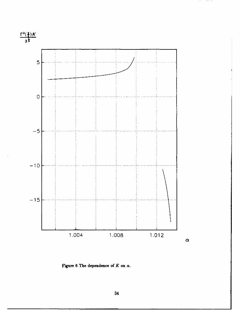
The next calculation required concerned the constant 92, defined by (2.20). In order to

calculate Q, from (2.20) it is necessary to compute the adjoint function J = (M, N, S, T). In

fact it is easier to solve the problem for (ul, vj, Pl, A 1) directly and find the value of fl, which

enables all the required boundary conditions to be satisfied. It was easier to compute Q, in this

way because the system for (ul, v1,pl, A1 ) can be solved using essentially the same iteration

method as used above for the solution of (2.12). In Figure 6 we show the dependence of K on

the wavenumber a. The fact that K is singular at a = a, = 1.0145 is a direct consequence of

the fact that W(a,) = 0. In Figure 7 we show the dependence of A0 on a and we observe that

A0, is respectively negative and positive on the lower and upper branches of Figure 3. Here

the upper and lower branches correspond to points on Figure 3 which are respectively above

or below E. The singularity in Ao,0 is due to the fact that A0 continues to decrease when a

passes through a,. The fact that both K and A0, change sign at a, means that viscous effects

have essentially the same destabilizing role on the upper and lower branches when uniform

wavetrains are considered; see the following section.

Now let us discuss the implications of our calculations for the evolution equation (2.22)

which we recall determines the wavenumber a correct upto order 63. The term on the right

hand side of (2.22) is due to viscous effects and the results of Figures 6, 7 imply that viscous

11

effects are destabilizing. The zeroth order approximation to (2.22) yields

T + = 0 (3.4)

where wg is the group velocity. We see from Figure 3 that the group velocity is negative for

the upper branch and positive otherwise. This suggests that the upper branch solutions are

physically irrelevant since their energy propagates upstream. In fact, the form of Figures 2,3,

and the known result about the stability at small amplitude of Tollmien-Schlichting waves,

Smith (1979b), suggests that solutions corresponding to the upper and lower branches would

be found to be unstable and stable respectively if a Floquet analysis of them were carried out.

Suppose then that we consider the evolution of disturbances cOrresponding to the lower

branch of Figure 3. If at T = 0 we are given

a = &(X)

then for T positive we have

a = &(X-w 9 (a)T)

which determines a implicitly since wg is a function of a. It is well-known, eg Whitham

(1974), that for positive w. the above solution will become multivalued after a finite time if the

initial data has a compressive part. This suggests that finite amplitude Tollmnien-Schlichting

waves will develop discontinuities in wavenumber and frequency as they propagate downstream.

When such shocklike structures develop (3.4) is no longer valid, and the viscous term must be

brought into play. We expect that the situation then is similar to that for Burgers equation,

see Whitham (1974), where viscous effects smooth out shocklike solutions but do not prevent

their development. However until a numerical treatment of (3.4) is carried out such remarks

should be treated as speculative. Now we shall concentrate on a case where more analytical

progress is possible and investigate nearly uniform wavetrains.

12

4 Uniform wavetrains and their stability

Suppose that (ao, Qo(ao)) is some point on the curve shown in Figure 3. The corresponding

wave with

E = O(aoX - 0o(ao)T)

corresponds to a constant frequency/wavenumber solution of the full 2D triple deck problem

for Tollmien-Schlichting waves. The stability of this system can be readily investigated by use

of the phase equation (2.22). We first write a = ao + A, where A is small, and then (2.22)

becomes

OA 9A t A X A---- + fo(ao)- + fol(o)A = -b 11 K(ao) -" AX dsWT_ OX OX 0OYa OX J00 1(3

+0(61/3A2, A3 ).

Note that KAo, is negative on both the lower and upper branches respectively of Figure 3.

We can eliminate the term proportional fl'(ao) by an appropriate Galilean transformation.

If we then take T = 0(6-1/3), A ,,b1/3 with X = 0(1) then, the limit 6 -+ 0, a suitably

rescaled version of the above equation is

OA OA 19 8A- + A- =(-- 6_/ ds. (4.1)0--7 + ý of it (S - ý)1/3

Therefore the longwave instability of a uniform wavetrain of Tollmien-Schlichting waves is

governed by the apparently new evolution equation (4.1).

Suppose now that at r = 0 there exists a small initial perturbation A = Ao(ý). The

linearized form of (4.1) shows that A evolves according to

A = / A*(k) exp [iki + A~ 1d2z _ )0 I r(2/3)(ik)2/3]

where A* is the transform of the initial data and

{e- i/ 3 k- 2/ 3 , k > 0,

(ik)-2 /3 =_

7613Ik- 2/3,e rJ3k[- /, k <O.

It can be seen that the ultimate form of the disturbance depends on A•(k). More precisely

we see that when Ao(ý) is sufficiently concentrated the solution will develop a singularity

at a finite time. Thus for example an initial disturbance of Gaussian form will have A• ,

exp(-k 2 ) and a bounded sol tion will occur for all time. However if A• ,, exp 1k 41/ 3 the

solution will become unbounded after a finite time. This is an important result because it says

that a constant wavenumber/frequency solution of the two-dimensional triple-deck problem for

13

Tolimien-Schlichting waves is always unstable to a long wave instability. This is not uncommon

in physical problems, eg the Stokes water wave, nonlinear optics. For a discussion of such

modulational instabilities the reader is referred to Whitham (1974).

A possible structure for A when this singularity is encountered is obtained by writing

A = (: - *(), -0I - 73/4

where the singularity occurs when r -: F and is localized around • - •. The constant A will

depend on the initial conditions, but we expect that only solutions with A > 0 w: -ossible.

The function %F is then found to satisfy

L4d d! 34 d %P0 ''(0)4 d do - 0J)1/3 (4.2)

We seek a continuous solution of (4.2) with P= 1@0, a constant, for 4) > 0 and allow ' to grow

algebraically when 4) -- o -o. It is then convenient to write or = -4) and let

C(0) = *(-a,) = 0 I {f(a) + 0}

so that f(a) satisfies

3 d(f f'(t)dtA{f( A)+1}- f(a)= T co(att)1/3' -0 <a <00,

and then f(or) = 0, a < 0, whilst for a positive f is determined by

P If (a) - 1- a(a)I=4 d fU f'(t)dt3da J (r - t)1/ 3 " (4.3)

When p = 4A/3 = 4/3 this equation has an exact solution proportional to a4 /3. If this solution

is written in terms of the original variables we obtain

J 0, > 0,

(4.4),@0 + s,•-"* _0J ' 4) <0,

For other values of p we can find a solution of (4.3) by taking a Laplace transform. After some

calculation we find that f (a) may then be written in the formS[.•+o e'PQ(p)d.

f = (o ri) C (p) ap, (4.5)

where

A(p) = pP+e-r(213) 4/3, Q(p) = 1 -q e- dq.

It is then easy to show from (4.5) that when a -- oo

f(a) -• a'.

14

Thus in terms of the original variables we obtain

which incidentally confirms the exact solution (4.4). Thus we have constructed solutions of

(4.2) for which i is singular with 0 < A < 3/4 whilst the solution for A = 0 corresponds tod46

a finite jump in * between 0 = ±-o00 so that the wavenumber perturbation (and therefore the

associated velocity displacement function) has a shock structure.

In the absence of a full numerical investigation of the evolution equation (4.1) we cannot

say which of the singular solutions will be excited. Indeed nothing in our discussion so far

has ruled out the possibility of finite amplitude equilibrium solutions of (4.1). However, if we

multiply (4.1) by X and integrate from ý = -co to ý = +o0, and use Plancherets formula to

simplify the contribution from the right hand side of (4.1), we obtain

o, X 2 (•, T)d• = v/j rl/ 31X*(r, r)1 2dr (4.6)

where X* is the Fourier transform of X. It follows from (4.6) that equilibrium solutions

(constant or in the form of traveling waves) are ruled out.

Breakdown of the full nonlinear problem

Now let us consider a possible breakdown form for the full nonlinear system (4.1). If the

breakdown is governed by the inviscid form of the equation then, following Brotherton-Ratcllffe

and Smith (1987), we can, after a suitable shift of origin, write

A = IrI' 1Qo(i,) + ...

with q = . The term on the right hand side of (4.1) is then negligible for n < 3/4 and Qo

is then given implicitly by

S= -Qo - eoQ0, (4.7)

with eo a positive constant. However (4.7) only determines Qo as a single-valued function of ilLwhen n = L- ' L = 3,5,7,... so that this type of structure is not possible. However we can

take n = 3/4 in which case Qo satisfies

-77Qo+-+QoQ= --- i) 0 Qo (ds. (4.8)4 4 O'J? a~s

The above integral equation must then be solved numerically. We postpone that numerical

investigation until we have carried out full numerical simulations of (4.1); such an investigation

will be reported on in due course.

15

5 A direct evaluation of the wavenumber modulation equa-

tion

We shall now use a multiple scale approach to derive (4.1) directly from the two-dimensional

triple deck equations (2.1). Again the major effect of the modulation is to introduce a layer

of depth 6-/3 sitting on top of the lower deck. We again define slow variables X and T by

writing

X = 6x (5.1a)

T = t. (5.1b)

It is then convenient to define X, Y by

2 = X -wT, (5.2a)

t = . 113T, (5.2b)

where wg is a group velocity to be determined at higher order in our expansion procedure.

Suppose then that we seek a solution of the triple-deck equations which is periodic in 40 =

ax - flt where a and Q are now taken to be constant. In the lower deck we expand U in the

form

00 = n/3Bn(XT) On 0 [U4 (0,,71 ,xt)n=O

+ b5/ 3 us(0,, y~, T) +... (5.3)

together with similar expansions for v and p. We note at this stage that the summation term

in (5.3) arises because of the translational invariance of a solution of the two-dimensional

triple-deck equations. In addition we note that the first correction to the underlying mean

state dependent on X arises at O(b4/3) in (5.3). It should also be stressed at this stage that

uo, the 0(1) term in (5.3), is independent of the slow scales X and T and that B(X, t) is an

amplitude function to be determined. Thus in (5.3) we identify the term /3Bo all04o

amplitude perturbation to the periodic flow uo(o, y). The eigenfunction O occurs because

of the translational invariance of any 4-periodic solution of the triple deck problem. For our

purposes here it is sufficient for us to consider the partial differential equations to determine

(u4 ,v 4,p4) and (u5,v 5, ps). If the expansions for u,v,p are substituted into the triple deck

equations, and the appropriate change of variables made, then we find that (u4, v4, P4) satisfies

a - B), Uoo, (5.4a)

02u 4 Op4 Ou4 OU0 OuO OU42 - - aUo80 - au410 - V4 y - voy - [-wguo + auouoo] B,1 .(5.4b)

16

These equations must be solved subject to U4 V 4 0, y = 0 whilst for large y the appropriate

conditions are

U4 A(O, X, T), (5.5a)

withoo A

= _1 T ds (5.6a)

Since the homogeneous form of the system for (u4 ,v4,p 4 ) has the solution (u4,v 4,p 4) =

-(uo, vp) it follows that a solution exists only if an orthogonality condition is satisfied.

This may be written down following the procedure used in §4, it is sufficient here to note that

the condition determines the group velocity w. and that the expansion obtained is identical to

that which it was derived in §3 after making a perturbation in the wavenumber. The solution

of (5.4) is clearly of the form

(U4 , V4 ,P 4 ) = BfC(U 4 , V4, P4), A = BfC A,

where (U 4 , V4, P4) and A are independent of k, T. The other main feature to appreciate about

the solution of the 0(6b/4) problem is that at the edge of the y = 0(1) region U4 may be

expressed in the formU4"A = (AM + AF(•b))B±

where AM is independent of 40 and therefore corresponds to a mean flow correction. The

reduction to zero of AM is achieved in the outer 0(6-1/3) region in a similar manner to that

found in §3. We define the variable 17 by

77 = 61/3y

and in the outer 6-1/3 layer u is expanded in the form

U / E ) + 64 13 UM(X 6)+ b513US ..+n=1

where UM is the mean flow correction driven by AM. The mean flow correction in the 11

direction is 62VM and the linear problem to determine (UM, VM) is found to be

OUM OVM-2 + --- =0,

0 2UM _ OUM

042 7) x- VM = 0,

UM = AMBX,VM =0,rI=O (5.7)

UM *0,1- 00.

The system (5.7) is identical to that obtained in Section 2 and therefore may be solved again

using a Fourier Transform technique, the solution is not repeated here. The mean flow at order

17

6413 then interacts with the O(6P) flow to produce an 0(65/3) correction to the outer boundary

condition for the disturbed flow in the y = 0(1) layer. Again the analysis follows closely that

of §2 so we do not repeat it here, we find that (us, vs,p 5 ) must satisfy

0Us A5 + -Jd,• OX (x - z)1/ 3

where A is a constant. In the y = 0(1) region (Us, v5 ,p5 ) is found to satisfy (5.4a,b) but with

the right hand sides of these equations replaced by [.], and

+Buo + BB VU4 +4uo+ VO__u4 +..+}

respectively. Here [.] denotes terms which don't contribute to the solvability condition which

the system for (u5 , v5 , P5) must satisfy. The required condition is

OH OH 9 ____LB

+ _-_ 9S(, T) ds, (5.8)OT OX- OxJ (S-

where g9, A are constants and a suitable change of variables enables us to recover (4.1). Thus

r in (4.1) can be interpreted as being either a wavenumber or amplitude perturbation and the

two approaches are shown to be consistent.

6 The phase equation approach at finite Reynolds numbers

In §2 we derived the phase equation for Tollmien-Schlichting waves in a Blasius boundary layer.

Such a boundary layer exists only at asymptotically large values of the Reynolds number and

it was therefore appropriate to utilize the largeness of the Reynolds numbers in the description

of the instability wave. However linear descriptions of the evolution of Tolhinien-Schlichting

waves at finite Reynolds numbers have been given by for example Gaster (1974). Though such

approaches do not give formal asymptotic approximations to the equations of motion it appears

that they correctly predict the essential physics of the linear growth of Tollmien-Schlichting

waves. Similarly large scale numerical simulations of nonlinear growth of Tolhmien-Schlichting

waves at finite Reynolds numbers have proved equally successful at reproducing experimental

results, e.g Wray and Hussaini (1984). Here we wish to investigate the phase equation approach

at finite Reynolds numbers but, in order to keep our asymptotic analysis formally correct, we

choose to work with a parallel boundary layer which is an exact solution of the Navier-Stokes

equations at all Reynolds numbers. We refer to the asymptotic suction boundary layer which

has been investigated in the weakly nonlinear regime by Hocking (1975). Suppose then thatV0the freestream speed is U0 and the suction velocity is V0. We define a reference length L -- -

and define the Reynolds number V0

R U0

Vo

18

but we assume that R = 0(1) in this section. Since we restrict ourselves to two-dimensional

disturbances it is convenient for us to define a stream function T and work with the vorticity

equation in the format + rVi/)4 (6.1)

which is to be solved subject to

O/y = 0, •/•=1, y 0 , (6.2a)

1,, ---+ 1, Y "-+ oo (6.2b)

In the absence of an instability the stream function 0 is given by

' = 0o(y) = Y + ey - X. (6.3)

This flow is unstable to two-dimensional Tollmien-Schlichting waves for R > 54370.0 and the

band of unstable wavenumbers tends to zero when R - oo. Here we assume R is 0(1) and

assume that an 0(1) amplitude wavesystem is superimposed on (6.3). At finite R the mean flow

driven by the wave system is confined to the boundary layer. Therefore no outer adjustment

layer is required even when the wavesystem evolves slowly in the downstream direction, see

Hocking (1975) for a discussion of this point. Suppose that X, T are defined by

X=x, T = t,

then we define0 =O(X, T), a• = Ox, 0 =-OT,

and expand R in the form

R = 110 + •fQl +'". (6.4)

We seek a solution of (6.1) by writing

, = ,Po(X, y, O,T) + 6bo(X,y,O,T)1-...

and the leading problem is determined by solving

f o .V 0 O(V 210 , 0 0) 10o 0(0,y) R

VboY = 0, alkoe = 1, y= 0, (6.5)

oY -* 1, y- -- 00,

with02 29

9y2 002,

19

and periodicity in 0. The required frequency and wavenumber, flo and a, must be found

numerically once some measure of the disturbance size is specified. We will not attempt such

a calculation here but we note from the finite Reynolds number calculation of Hocking (1975)

and the large Reynolds number theory of Smith (1979a,b) that both sub and supercritical

bifurcations to finite amplitude Tollmien-Schlichting waves are possible. For the purposes of

our discussion we simply assume that the nonlinear eigenrelation flo = flo(a, R) is known. At

order 6 we find that V/, is determined by

OV2~I p a('O, V2, 1) O(Ip' V,0?40) 1- -V 4 1' -= vfl '0 I O 8-00 = -+ -M(0,X,y). (6.6)o 0 0(0, y) o(0, y) R 8X a ,

whereM ( 0o,V•'o) V2 20 (o, 2 ackae) 4a 028 (a, y) 0(0, Y) R naO 1~oV o

The system must be solved subject to periodicity in E whilst the boundary conditions in y

are

01 = 0, y=O (6.7a)

0/1 -- q(X), y - 00. (6.7b)

Here q(X) represents a mean flow normal to the wall at infinity. This flow is essentially

driven through the equation of continuity by the 0(1) streamwise velocity component. A solv-

ability condition is required if (6.6)-(6.7) is to have a solution since the translational invariance

of (6.5) means that ii = 0•0 is a solution of the homogeneous form of (6.6)-(6.7). It is worth

pointing out at this stage that, if we were performing a calculation in a region of finite depth,

then a pressure eigenfunction would have to be allowed for at leading order in order that q

should be reduced to zero. The requirement for such an eigenfunction is well-known in weakly

nonlinear stability theory; see for example Davey, Hocking and Stewartson (1974) or DiPrima

and Stuart (1975). The solvability condition can be found by writingS=(, aV'e, OY, V20, aV20o, VOY)T

in which case the homogeneous form of (6.6) is

a aaý-6AZ-+---YBZ+CZ=O,

where A, B and C are 6 x 6 matrices defined by

10000 0

0 0000 0

0 1 0 0 0 0000100

000000

000010

20

000000

1000000 001000

B=000000

000 100

000001

0 -1 0 0 0 0

0 0 -1 0 0 0

o 0 0 -1 0 0C = 0 0 0 0 -1 0

0 0 0 0 0 -10 -RV1,oy aRVoe 0 R[ako, -0] -R0,b0 e

The system adjoint to that given above is

- ATQ- !yBTq + CTQ - 0, (6.8)

together with conditions of periodicity in 0 and

q5 = q6, y = 0, oo. (6.9)

The condition that (6.6)-(6.7) has a solution then becomes

oa= f, (6.10)

with 2w

fl = f0 ' M(E),X,y)q6dOdy

fo1 f0 L-Vq 6dOdy

The phase condition fnx + aT = 0 correct upto 0(b) becomes

aT + aXC O(a) = a {lax fA(a)l6b (6.11)

In order to examine the stability of a uniform wavestream solution we write

a = ao + A

with A << ao, and (6.11) after a suitable change of scales becomes

A, + AAt = ±At. (6.12)

Thus we obtain the surprising result that the modulational instability of a two-dimensional

wavesystem in a boundary layer at finite Reynolds numbers is governed by Burgers equation.

21

In (6.12) the ± signs correspond to the cases when diffusion effects are stabilizing/destabilizing

respectively. Without calculating Q, we do not know which sign is appropriate for the problem

under consideration here so we will discuss both possibilities. However we can simply quote

the known results about Burgers equation for each case and the implications for the stability

of a uniform wavetrain are essentially the same. A full discussion of results quoted below can

be found in Whitham (1974) and Howard and Kopell (1977).

If the positive sign is taken the solution remains bounded for all time and indeed localized

or periodic solution of (6.12) tend to zero when T increases. However even in the diffusively

stable case weak shock solutions of (6.12) can develop; a discussion of this possibility is given

by Whitham (1974), Howard and Kopell (1977). Thus for any giten uniform wavetrain whose

instability is governed by (6.12) with the positive sign, an initial disturbance can be found

which does not decay to zero at large times. The uniform wavetrain is therefore modulationally

unstable.

If the negative sign is taken in (6.12) viscous effects are destabilizing and in fact finite time

singularities are developed from a broad range of initial conditions. Again it follows that the

uniform wavetrain is unstable.

We conclude that at finite Reynolds numbers modulational effects will either cause a finite

time singularity to develop if viscous effects are destabilizing, or cause shock discontinuities

in wavenumber and frequency in the stable case. In either case uniform wavetrains of two-

dimensional Tollmien-Sclichting waves at finite amplitude should not be observed according to

our theory.

7 Conclusion

We have used a phase equation approach to determine the evolution of Tollmien-Schlichting

waves at large and finite Reynolds numbers. In the high Reynolds number case we found that

finite amplitude disturbances, periodic in time and space, apparently exist only for a small

range of values of the wavenumber a. The upper branch in Figure 3 describes modes with

negative group velocity and so they are therefore of no physical interest. The lower branch on

the other hand corresponds to waves with positive group velocity and for these modes the rate

of change of the group velocity with a is positive. This means that (2.22), the leading order

approximation to the phase equation, will develop discontinuities after a finite time for many

initial disturbances. It might be anticipated that viscous effects, which appear on the right

hand side of (2.22), might smooth out such discontinuities. We cannot be sure if that is the

case until a numerical investigation of (2.22) is carried out. However, in §4 we investigated the

particular case of uniform wavetrains and found that there viscous effects were destabilizing

and it seems likely that this is also the case for (2.22). In §4 we saw that the linearized form

22

of (4.1) leads to a finite time singularity of the type found by Brotherton-Ratcliffe and Smith

(1987). For the full nonlinear problem (4.6) shows that equilibrium solutions are not possible

and that ,n initial perturbation cannot decay to zero at large times. In effect this means that

periodic solutions of the triple-deck equations are miodulationally unstable. A possible form for

the structure of a singular solution of the breakdown of the nonlinear form of (4.1) was found.

The structure found was again based on the structure found by Brotherton-Ratcliffe and Smith

(1987). The validity of the structure must remain open until a full numerical investigation of

(4.1) has been carried out. The question of how the Navier-Stokes equations alter their large

Reynolds number structure in order to remove the singularities of (4.1) also remains open.

At finite Reynolds numbers we found that the evolution equation for a periodic wavetrain

satisfies Burgers equation. Without extensive calculations we cannot say whether the viscous

term in (6.12) has positive a or negative sign. If it turns out to be negative then viscous effects

are again destabilizing and finite time singularities will occur. If the sign is positive then viscous

effects are stabilizing . However (6.12) can be solved exactly by the Cole-Hopf transformation

and it is known, Whitham (1974), that even in the stable case shocks will in general develop.

Thus we conclude that at large or finite Reynolds numbers a uniform wavtrain of Tollmien-

Schlichting waves will break down with a singularity or shock developing after a finite time.

This casts some doubt on the validity of large-scale simulations of Tollmien-Schlichting waves

using Fourier series expansions in the streamwise direction.

In view of the fact that our analysis has been restricted to the two-dimensional case it

is possible that three-dimensional effects might prevent the above predictions from occurring

in practice. Nevertheless, experimental observations where the Tollmien-Schlichting wave is

driven by a wavemaker suggest that the first step in the transition process is the linear growth

of two-dimensional Tollmien-Schlichting waves followed by nonlinear saturation and three-

dimensional effects coming into play, see for example Klebanoff et al (1962).

As a first step towards looking at the effect of three-dimensionality let us determine how

the evolution equations (4.1), (6.12) are modified if a weak spanwise dependence of the wave

is allowed for. We shall determine the modifications using the multiple-scale approach of §5

rather than modify the phase equation formulation. Since §5 concerned Tollmien-Schlichting

waves at large Reynolds number let us give the essential details of how the corresponding

expansion procedure is formulated at finite Reynolds numbers. In the absence of spanwise

modulation the streamwise velocity component is written in the form

U = oE aQf&A"(fC,T)8`uO(O'y) + b 2 u2 (O,y, fT) + b 3 u3(0,y, Y , T)+... (7.1)

Here X = 6(x - wrt) is a slow variable obtained by moving to a coordinate system moving

downstream with the group velocity and a = ax - Q0t. The summation term arises because of

23

the translational invariance of a periodic solution in the streamwise direction. At order 62 the

group velocity is determined as a solvability condition and u 2 will be proportional to Af,. At

order 6' terms proportional to AAg and a slow time derivative of A will be generated. Viscous

effects also come into play to generate terms proportional to Af) and the require(] solvability

condition leads us to (6.12). In the presence of spanwise modulations the procedure described

above is modified in the following way. Firstly we define a slow variable

( = bz

where z is the spanwise variable and allow the amplitude function A to depend on C. The above

expansion for u remains unchanged but the O(6) term in the corresponding pressure expansion

drives a spanwise flow of order b2 proportional to A(. This spanwise velocity component then

generates a term proportional to A(( in the O(P3) continuity equation. Similar terms are

generated by spanwise diffusion in the x, y momentum equations. The solvability condition

then is modified to give

A, + AAt -: ±At + AA(. (7.2)

Here A, is a constant whose sign cannot be calculated without solving the 0(1) problem

numerically. A similar analysis for the triple-deck case gives

OAX OA = 0 ___

- + - '2' ds + A2A((. (7.3)Or- + 9 A9 t•= O (s - 0)111

with A2 a constant as the required generalization of (4.1). As a starting point to study the role

of three-dimensional effects in the two-dimensional breakdown structure w- plan to carry out

numerical simulations of (7.2), (7.3).

Finally we close with a brief outline of how (2.22), (4.1) are modified by nonparallel flow

effects. Within the framework of (2.1) nonparallel effects manifest themselves through the

pressure displacement law which allows for elliptic effects in the streamwise direction. However

the slow spatial evolution of the unperturbed shear flow does not enter (2.1) since it can be

scaled out of the problem. For the weakly nonlinear growth of Tollmien-Schlichting waves

Hall and Smith (1984) showed that nonparallel effects are important when the disturbance

amplitude is O(R- 7/3 2) and lead to an amplitude equation of the form

dC = XC_ -(1 + iW)CICI 2, (7.4)dX

with ý a real constant. Thus nonparallel effects lead to the term XC in (7.4) thereby causing

the increased linear exponential growth of a small disturbance as it evolves in X. Any small

disturbance amplifying by this means eventually becomes nonlinear and for large X has 1C12

X. Let us now show how related terms can be incorporated into (2.22) and (4.1).

24

We note that (2.11a) proceeds in powers of 63 and that the Reynolds number has been

effectively scaled out of the problem by our assumption that the Tolhnien-Schlichting wavesys-

tern is described by the triple-deck system (2.1).This assumption means that the analysis given

so far in this paper is formally valid for b large compared to any positive power of f = R- 8. In

order to reveal the effect of boundary layer growth we now relax this condition and see which

new terms now play a role in (2.11a). Clearly (2.11a) must include terms proportional to

powers of f because of the higher order terms in the triple deck expansion but in addition there

will be a term proportional to E3 -1 X obtained by expanding the streamwise dependence of

the unperturbed flow in a Taylor series in the streamwise direction. We therefore now expand

the frequency in the form

Q = Q0 + 61/ 3 SI, + E?2 + E2f2 3 + E3 b-1Xfl4 + 0(E 3, F 63 2 ,E6b )• (7.5)

The ordering of the terms in the above expansion depends on the relationship between 6 and t.

The term proportional to f?4 is the first one dependent on the nonparallel nature of the basic

flow. The first significant distinguished limit arises when 6 , f when the terms proportional to

9341 4 become comparable but still small compared to the O(b3) term. The next significant

stage is when 6 decreases to J in which case the nonparallel term and the 0(63) term are9

comparable. However the crucial stage arises when 6 decreases to 0 in which case the terms

proportional to f?1, f14 play an equal role and viscous and nonparallel effects are comparable.

Thus if we write

3

with hi an 0(1) constant then (2.2), correct to second order, now gives

8a O9Qo O9a on ,1/.Off4O+ _-F ax - 61/3( +- hlfl4+ -nX ... ) (7.6)

A further decrease in the size of 6 means that the term proportional to 9 1 should be dropped

and nonparallel effects dominate the right hand side of the equation for a. This completes our

description of how the phase equation changes its structure Ahen 6 is decreased. Note here

that when we decrease 6 we are in effect moving further away from the initial location x* = i*

so the above different orderings of the right hand sides of (7.5) correspond to moving further

downstream. Thus the final form has the right hand side of the phase equation dominated by

nonparallel effects.

A similar procedure can be used to determine the appropriate modifications to (4.1) which

is the evolution equation for the perturbed wavenumber of an initially uniform wavetrain. Here

the crucial scaling brings in nonparallel effects at the same stage as the integral term driven

by viscous terms. The appropriate scaling now has

f 3 h2 =

25

with h2 an 0(1) constant. Equation (4.1) then becomes

8A 8A I __!A_

- (A + h37r '9 " ds + h4 . (7.7)19- A r- S - )1/3

Here h3 , h4 are constants proportional to h2, and h4 can be set equal to zero by a change of

dependent variable. Therefore the nonparallel modulational equation for ToUlmien-Schlichting

waves in a growing boundary layer is (7.6) with h4 = 0, the numerical solution of that equation

will be reported on in due course.

The author would like to thank Professor T. Conlisk and Professor F. T. Smith for dis-

cussions concerning Conlisk, Burggraf and Smith (1987). The author also benefitted from

conversations with Dr. P Duck, Dr. J. Gajjar, Dr. Paul Martin, Dr. A. Ruban. Finally the

author would like to thank Professor R. E. Kelly for his hospitality and encouragement when

this work was started.

26

References

Brotherton-Ratcliffe, R. V. and Smith, F. T., 1987, Mathematika, 34, 86.

Conlisk , A.T., Burggraf, O.R., Smith, F.T. 1987, Trans ASME FED, 52, 119.

Cross, M., Newell, A.C. 1984, Physics D, 10, 299.

Davey, A., Hocking, L. M. and Stewartson, K. 1974, J. Fluid Mech., 63, 529.

DiPrima, R. C. and Stuart, J. T. 1975, J. FLuid Mech. 67, 85.

Gaster, M. 1974, J. Fluid Mech., 66, 465.

Hall, P. 1988, J. Fluid Mech., 193, 243.

Hall, P. and Smith, F.T. 1984, Studies in Appl. Math. 70, 91.

Herbert, T. 1977, AGARD Conference Proceedings CP-224, 3/1-10.

Howard, L. and Kopell, N. 1977, Studies in Appl. Math. 56, 95.

Hocking, L. M. 1975, QJMAM 28, 341.

Kachanov, Yu. S. and Levchenko, V. Yu, 1984, J. Fluid Mech. 138, 209.

Khokhlov, A. P. 1994, J. Applied Math. and Tech. Physics, 34, 508.

Klebanoff, P. S., Tidstrom, K. D., and Sargent, L. M., 1962, J. Fluid Mech. 12, 1.

Kramer, L., Ben Jacob, E., Brand, H. and Coss, M. C., 1982, Phys. Rev. Lett. 49, 1891.

Lin, C. C. 1966, The Theory of Hydrodynamic Stability, CUP.

NeweU, A.C., Passot, T. and Lega, J. 1993, Ann. Rev. Fluid Dynamics. 25, 399.

Smith, F.T. 1979a, Proc. Roy. Soc. (A) 366, 91.

Smith, F.T. 1979b, Proc. Roy. Soc. (A) 368, 513.

Smith, F. T. and Burggraf, 0. R., 1985 Proc. Roy. Soc (a), 399, 25.

Smith, F.T. and Stewart, P. 1987, J. Fluid Mech., 194, 21.

Whitham, G. B. 1974, Linear and Nonlinear Waves, Wiley.

Wray, A. A. and Hussaini, M. Y., 1984, Proc. Roy. Soc. A 392, 373.

27

FIGURESFigure 1 The dependence of c• on cj + do2.Figure 2 The dependence of a?0 on + + do.

Figure 3 The dependence of Co on a. The symbols denote the results of Conlisk et al.

Figure 4 The shear stress as a function of 9 for go0 = 2.2995,2.3041,2.3125,2.3245,2.3398,

2.3575,2.3763,2.395,2.4124,2.4275

Figure 5 The shear stress u' (0) as a function of g~o for the first sixteeen modes.

Figure 6 The dependence of K on a.

Figure 7 The dependence of Ao on a.

28

0 .3 5 .4. .......... ..........................

0 .3 0 ! .. ................................... ........ .. . .... ............... ...... ....... ..... ..... .

0 .'; ......... ............................ ....................................... .......... .. .

0 .2 0 .. ....... .... ... ... .

0 . 1 5 ... ................................................ .... ............ ......................

0.10

0.05 ...

0.00

1.000 1.004 1.008 1.012

Figure 1 The dependence of a on A "do.

29

0.35 - ."

0.30

0.25

0.20

0.15...............

0.10

0.05 ............. .......................

0.00........ . . . . ....................... .....

2.32 2.36 2.40•o

Figure 2 The dependence of % on 0 + d.

30

Q00

.00

2 .4 2 ..... ... . . . . .. . .. ... . . .

2 .4 0 ... . .. . . .. . . . . . . .. . . .£.. .

2.36.. .. ............... .... ........... .....

1.000 1.004 1.008 1.012

Figure 3 The dependence of flo on a. The symbols denote the results of Conliak et al.

31

tLOv

1 .4.. .... ... ......

1 .0

0.2 ...... ..... ......1...m m

0 m

Fig re 4..e.he r .tre... function................ of..... .for ... . .....230 1, .3 5, .3 4.. 33..,

Figr34575,2 er.376s3s,2.ncionof395r,2.4.99,230242312,.3427.398

32

10g1U1'on(O)I _ _ _ _ _ _ _ _ _ _ __ _ _ _ _ _ _ _ _ _ _ _

-5 m increasing

--------

-1 5 . . . .. . ....

- 1 5 . . .......... ...... ...... ....

Figur 5.The.shear.strss..........a... ....tion of....for.the.first....teee. mo e . ....

- 3 ... .. .. .. .. .. .. ..... .. .. ... .. .. .. ... . ...3.

r 2( )K

35

5 . . . . . . . . . . . . . . . . . . . . . . . . , .. . . . . . . . .. , . ... . . . . . , . . . . . . . . . . . .. . . . . . . .. . . . . . . . .. . . . . ..

• 5 .... ... .... ... ... ......................................... ................... ...............

- 1 0 ........ ... ............ .............. .............. •............... .............. .. . . . . .

-15

II , I I I

1.004 1.008 1.012

Figure 6 The dependence of K on a.

.34

A0

0.00

-0 .0 2 .. ... . ...............

1.004 1.008 1.012

Figure 7 The dependence of AO on a.

35

ROIForm ApprovedREPORT DOCUMENTATION PAGE I OMB No 0704-0188

Public reporting burden for this collection of information is estimated to average I hour per response, including the time for reviewing instructions, searching existing data sources,gathering and maintaining the data needed, and completing and reviewing the collection of information Send comments regarding this burden estimate or any other aspect of thiscollection of information. including suggestions for reducing this burden, to Washington Headquarters Services. Directorate for Information Operations and Reports, 1215 JefersonDavis Highway. Suite 1204. Arlingon. VA 22202-4302. and to the Office of Management and Budget, Paperwork Reduction Project (0704-0188). Washington. DC 20503

1. AGENCY USE ONLY(Leave blank) 2. REPORT DATE 13. REPORT TYPE AND DATES COVERED

April 1994 Contractor Report4. TITLE AND SUBTITLE S. FUNDING NUMBERS

A PHASE EQUATION APPROACH TO BOUNDARY LAYERINSTABILITY THEORY: TOLLMIEN SCHLICHTING WAVES C NAS1-19480

WU 505-90-52-01

6. AUTHOR(S)

Philip Hall

7. PERFORMING ORGANIZATION NAME(S) AND ADDRESS(ES) 8. PERFORMING ORGANIZATION

Institute for Computer Applications in Science REPORT NUMBER

and Engineering ICASE Report No. 94-23Mail Stop 132C, NASA Langley Research CenterHampton, VA 23681-0001

9. SPONSORING/MONITORING AGENCY NAME(S) AND ADDRESS(ES) 10. SPONSORING/MONITORING

National Aeronautics and Space Administration AGENCY REPORT NUMBER

Langley Research Center NASA CR-194901Hampton, VA 23681-0001 ICASE Report No. 94-23

11. SUPPLEMENTARY NOTES

Langley Technical Monitor: Michael F. CardFinal ReportSubmitted to Journal of Fluid Mechanics

12a. DISTRIBUTION/AVAILABILITY STATEMENT 12b. DISTRIBUTION CODE

Unclassified-Unlimited

Subject Category 34

13. ABSTRACT (Maximum 200 words)Our concern is with the evolution of large amplitude Tollmien-Schlichting waves in boundary layer flows. In factthe disturbances we consider are of a comparable size to the unperturbed state. W shall describe two-dimensionaldisturbances wh ich are locally periodic in time and space. This is achieved using a phase equation approach of thetype discussed by Howard and Kopell (1977) in the context of reaction-dif fusion equations. We shall consider bothlarge and 0(l) Reynolds numbers flows though, in order to keep our asymptotics respectable, our finite Reynoldsnumber calculation will be carried out for the asymptotic suction flow. Our large Reynolds number analysis, thoughcarried out for Blasius flow, is valid for any steady two-dimensional boundary layer. In both cases the phase equationapproach shows that the wavenumber and frequency will develop shocks or other discontinuities as the disturbanceevolves. As a special case we consider the evolution of constant frequency/wavenumber disturbances and show thattheir modulational instability is controlled by Burgers equation at fi nite Reynolds -number and by a new integro-differential evolution equation at large Reynolds numbers. For the large Reynolds number case the evolution equationpoints to the development of a spatially localized singularity at a finite time. The three-dimensional generalizationsof the evolution equations is also given for the case of weak spanwise modulations.

14. SUBJECT TERMS 15. NUMBER OF PAGESBoundary layer, phase equation 39

16. PRICE CODE

A0317. SECURITY CLASSIFICATION 18. SECURITY CLASSIFICATION 19. SECURITY CLASSIFICATION 20. LIMITATION

OF REPORT OF THIS PAGE OF ABSTRACT OF ABSTRACTU nclassified U nclassifiedI

SN 754111-01-80-580 Standard Form 298(Rew. 2-89)Prescribed by ANSI Std. Z39-18298-102