1 1W I I I

NASA Contractor Report 181914

ICASE Report No. 89-69

ICASE(Y)

q THE USE OF LANCZOS'S METHOD TO SOLVE THE1-" LARGE GENERALIZED SYMMETRIC DEFINITEN EIGENVALUE PROBLEM

Mark T. JonesMerrell L. Patrick

Contract No. NASI-18605September 1989

Institute for Computer Applications in Science and Engineering

NASA Langley Research CenterHampton, Virginia 23665-5225

Operated by the Universities Space Research Association DTICELECTEM

NASA NOV1719N9E' .ttrin-l Ap rnatlhc, and-;(),I( ( Ardlrirriqfration

Langley Research Center . . . .Ha plnn. Virqna 23665-5225

-MUI-VU'--__ 89 11 16 120. ... W JIMn,. "Lb ,mm ftn . I l l

Recently, ICASE has begun differentiating between reports with a mathemat-ical or applied science theme and reports whose main emphasis is some aspect ofcomputer science by producing the computer science reports with a yellow cover.The blue cover reports will now emphasize mathematical research. In all otheraspects the reports will remain the same, in particular, they will continue to besubmitted to the appropriate journals or conferences for formal publication.

iwl I I I III I I I

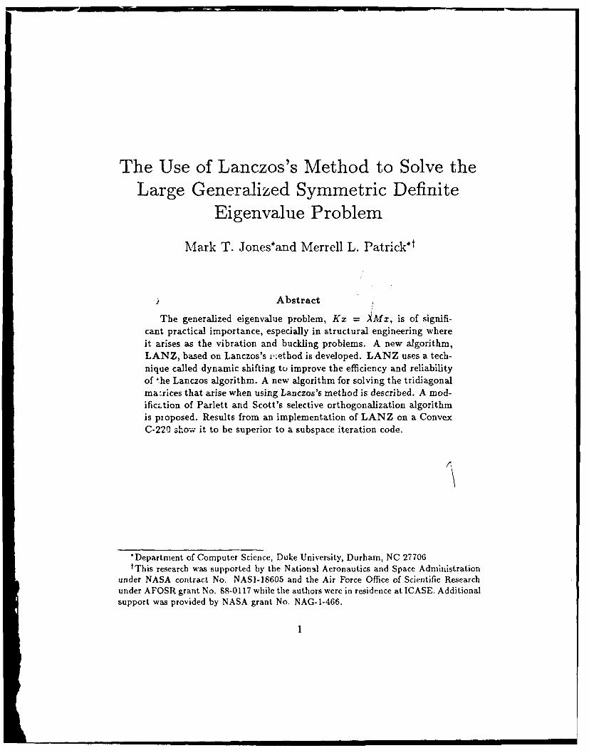
The Use of Lanczos's Method to Solve theLarge Generalized Symmetric Definite

Eigenvalue Problem

Mark T. Jones*and Merrell L. Patrick*t

Abstract

The generalized eigenvalue problem, Kx = XMx, is of signifi-cant practical importance, especially in structural engineering whereit arises as the vibration and buckling problems. A new algorithm,LANZ, based on Lanczos's i:ethod is developed. LANZ uses a tech-nique called dynamic shifting to improve the efficiency and reliabilityof the Lanczos algorithm. A new algorithm for solving the tridiagonalma:rices that arise when using Lanczos's method is described. A mod-ificztion of Parlett and Scott's selective orthogonalization algorithmis pioposed. Results from an implementation of LANZ on a ConvexC-220 show it to be superior to a subspace iteration code.

*Department of Computer Science, Duke University, Durham, NC 27706tThis research was supported by the National Aeronautics and Space Administration

under NASA contract No. NASI-18605 and the Air Force Office of Scientific Researchunder AFOSR grant No. 88-0117 while the authors were in residence at ICASE. Additionalsupport was provided by NASA grant No. NAG-1-466.

. ... mimmmmmAmio I illil~li~ii i •imim n mll I1

1 Introduction

The solution of the symmetric generalized eigenvalue problem,

Kr = AMx, (1)

where K and M are real, symmetric matrices, and either K or Af is positivesemi-definite, is of significant practical impor:ance, especially in structuralengineering as the vibration problem and the buckling problem 1BH87]. Thematrices K and M" are either banded or sparse. Usually p << n of the small-est eigenvalues of Equation 1 are sought, where n is the ordcr of the system.The method of Lanczos, suitably altercd for the generalized eigenvalue prob-lem, is shown to be useful for the efficient soiution of Equation 1. ILan50](NOPEJ87].

A sophisticated aleorithm, ha-pd on the ,;m-ple Lanczc -;shr, is

developed in this paper. The algorithm, called LANZ, has been imple-mented on supercomputer architectures at NASA Langley Research Centerand results from the implementation are discussed. Two applications fromstructural engineering are described in Section 2. The properties of the gener-alized eigenvalue problem and solution methods are given in Section 3. Thesimple Lanczos algorithm is presented in Section 4. The use of Lanczos'smethod for the generalized eigenvalue problem and the LANZ algorithmare discussed in Section 5. An execution time cost analysis of LANZ isdeveloped in Section 6. The solution of the tridiagonal matrices that arisewhen using Lanczos's method is considered in Section 7. Methods fcr solvingthe symmetric indefinite linear systems that arise in LANZ are described inSection 8. In Section 9, the performance of the LANZ algorithm is analyzedand compared to the performance of subspace iteration, the most prevalentmethod for solving this class of problems in structural engineering.

Accbssion ?or

DTIC A 0Unar-ou,! -d o

By.-

Ava. 18 :11 ty Codes 2SA,. &1 anid/or

Dist Special

2 Problems of Interest

Two important applications of LANZ which arise in structural engineeringare the vibration problem and the buckling problem. Practical problemsfrom these applications will be used to test the performance of the program.

In the free vibration problem, the vibration frequencies, w, and modeshape vectors, z, of a structure are sought. The equation

Kx = w2 MX, (2)

is solved, where K is the positive definite stiffness matrix and M is the semi-positive definite mass matrix. The mass matrix, M, can be either diagonal(in which case it is referred to as a diagonal mass matrix) or can have approx-imately the same structure as K (in which case it is referred to as a consistentmass matrix). Because K is positive definite and M is semi-positive definite,the eigenvalues of 2 are non-negative. When a dynamic load is applied to astructure, the structure begins to vibrate. If the vibration frequency is closeto a natural frequency of the structure, w, then the resulting resonance canlead to structural failure. Engineers want to ensure that a structure has nonatural frequencies near the range of frequencies of expected dynamic loads.Engineers are often interested in a few of the lowest frequencies of the struc-ture to ensure that these natural frequencies are well above the frequenciesof expected dynamic loads. [Jon89]. In some situations, all the frequenciesin a particular range may be sought. [Kni89].

In the buckling problem, the smallest load at which a structure will buckleis sought. These buckling loads of a structure, A, are the eigenvalues of thesystem,

Kx = -AKGx, (3)

where K is the positive definite stiffness matrix, KG is the geometric stiffnessmatrix, and x is the buckling mode shape vector [Mah87]. The KG matrixhas approximately the same structure as K and can be indefinite and singu-lar. Because KG is indefinite, the eigenvalues of Equation 3 can be negative,although in most practical problems they are positive. Equation 3 can haveup to n distinct eigenvalues; although only the smallest eigenvalue is of phys-ical importance since any load greater than the smallest buckling load willcause buckling [Jon89]. Designers may, however, be interested in the six toten lowest eigenvalues in order to observe the spacing of the buckling loads.

3

If the lowest buckling loads are greatly separated from other Ickling loads,the designer may seek to change the structure in order to cause the lowestbuckling loads to become closer to the other buckling loads of the structure.

[Kii89]. Because the IC matrix can be indefinite and singu!ar, the bucklingproblem is more difficult to solve numerically than the vibration problem.

4

3 The Generalized Eigenvalue Problem

3.1 Properties

Equation 1 yields n eigenvalues if and only if the rank of M is equal to n,which may not be the case in the problems under consideration [GL83]. Infact, if M is rank deficient, then the number of eigenvalues of Equation 1may be finite, empty, or infinite [GL83]. In practical problems, however, theset of eigenvalues is finite and non-empty. When K and M are symmetricand one or both of them is positive definite, the eigenvalues of Equation 1are real (without sacrificing generality, it will be assumed tbat M i!. positivedefinite). An orthogonal matrix, R, exists such that

RTM R = diag(fl) = D2 , (4)

where the fli are the eigenvalues of M and are therefore positive real. If Mis expanded to RD 2 RT, then Equation 1 becomes

(K - AM)x = (K - ARDDR T )x. (5)

Equation 5 can be rearranged to become

(K - AM)x = (RD(D-1 R T KRD- 1 - AI)DRT)x. (6)

Taking the determinant of each side yields

det(K - AM) = (det(R))2(det(D))2det(P - AI), (7)

where P = D-RTKRD- . Because R is orthogonal dei(R) = 1. Det(D) isthe product of the eigenvalues of M, which are all positive real. Therefore,the roots of det(K- A-M) are those of det(P- AI). Because P is a symmetricmatrix, its eigenvalues are all real and therefore those of Equation 1 are allreal [Wil65].

When K is positive definite and M is positive semi-definite, as they are inthe vibration problem, the eigenvalues of Equation 1 are all non-negative. Toshow that the eigenvalues are non-negative, multiply each side of Equation 1by xT to get

XT Kx - AXTMx. (8)

5

Because K is positive definite, xTKx is positive, and because Al is posi-tive semi-definite, xTMx is non-negative; therefore, A must be non-negative[Wil65].

The eigenvectors of Equation 1 satisfy M-orthogonality (xTMy = 0, if xand y are Al-orthogonal). The matrix, P, has a complete set of eigenvectors,zi, and the same eigenvalues as Equation I. Thus,

Pz1 = Ajz 1 , (9)

and,D-1RTIKRDlz = Aizi. (10)

Then, the sequence of transformations in Equation 11 show that x = RD-1 z,

KRD-1zj = ARDzj = AIRD(DRT RD-)zi = AM(RD-'zj) (11)

Because the zi are known to be orthogonal,

0 = zTzj = (DRT a)TDRT r = xAlx3 . (12)

The methuds and algorithms discussed in this paper rely on the eigenvaluesbeing real and the eigenvectors being M-orthogunal. In addition, LANZmakes use of the property that the eigenvalues in the vibration problem arenon-negative.

3.2 Solution Methods

Several methods for solving the large symmetric generalized eigenvalue prob-lem exist. A popular method, especially in structural engineering, is sub-space iteration [Bat82]. Nour-Omid, Parlett and Taylor provide convincingtheoretical and experimental evidence that Lanczos's method is superior tosubspace iteration on a sequential machine [NOPT83]. The parallelization ofsubspace iteration was investigated by Mahajan and it remains an open ques-tion as to whether Lanczos's method will be superior to subspace iterationon parallel machines [Mah87]. Another solution method for the generalizedeigenvalue problem is a two-level iterative method proposed by Szyld [Szy83].

He uses a combination of the inverse iteration and Rayleigh quotient meth-ods at the outer level, and an iterative solver for indefinite systems at theinner level. Szyld assumes, however, that Al is non-singular, which is not

6

always the case for the applications under examination. A promising methodfor parallel machines based on the Sturm sequence property is proposed byMa [Ma88]. He uses multi-sectioning or bi-sectioning to obtain the eigen-values, and then uses inverse iteration to recover the eigenvectors. Again,the assumption is made that M is non-singular. Schwarz proposes a methodwhich minimizes the Rayleigh quotient by means of the conjugate gradientmethod. The method uses a partial Choleski decomposition as a precon-ditioner to speed convcrgence [Sch89]. SOR-based methods have also beenproposed for the generalized eigenvalue problem, but these suffer from twoflaws: 1) the methods have difficulty when the eigenvalues are clustered, and2) the methods require that Ml be positive definite [Ruh74]. Other meth-ods have also been proposed [SW82] [Sch74]. Block Lanczos methods havebeen developed but are more complicated than the simple Lanczos process.Block methods are limited in that the user of the method must choose thesize of the blocks [NOC85]. One significant advantage of the block methodsis that they can easily reveal the presence of multiple eigenvalues [GU77].To the best of the authors' knowledge, no satisfactory method of choosingthis block size to best determine the multiplicity of eigenvalues has beenproposed. The block size is usually chosen to take advantage of a particularcomputing architecture [Ruh89].

7

4 Lanczos's Method

4.1 Execution in Exact Arithmetic

In order to understand Lanczos's method when applied to the generalizedeigenvalue problem, it is first necessary to examine the method when appliedto

Ax = Ax, (13)

where A is an n x n real symmetric matrix. In Lanczos's method, the matrixA is transformed into a tridiagonal matrix, T, in n steps in exact arithmetic.However, roundoff errors make the simple use of Lanczos's method as a di-rect method for tridiagonalizing A impractical [Sim84]. Palge suggests usingLanczos's method as an iterative method for finding the extremal eigenvaluesof a matrix [Pai7l]. At each step, j, of the Lanczos algorithm, a tridiagonalmatrix, T,, is generated. The extremal eigenvalues of Ti approximate thoseof A, and as j grows, the approximations become increasingly good [GL83].Both Kaniel and Saad have examined the convergence properties of Lanczosin exact arithmetic [Kan66] [Saa80). The convergence results that they de-rive imply that the speed of convergence of the eigenvalues of the T matricesto eigenvalues of A depends on the distribution of the eigenvalues of A; if anextreme eigenvalue of A is well separated from its neighbors, convergence tothis eigenvalue will be fast. However, clustered eigenvalues, or eigenvaluesthat are in the middle of the spectrum of A, will not be converged to asquickly as the extremal eigenvalues.

In Lanczos's method, a series of orthonormal vectors, q, ... q, is gener-ated which satisfy:

T = QTAQ, (14)

where the vectors qj are the columns of Q. If each side of Equation 14 ismultiplied by Q to yield,

QT = AQ, (15)

and the columns on each side are set equal, then

o3+lqj+l + qjai + qj-10j = Aq.. (16)

where the ca's and O's are the diagonal and subdiagonal, respectively, of T,

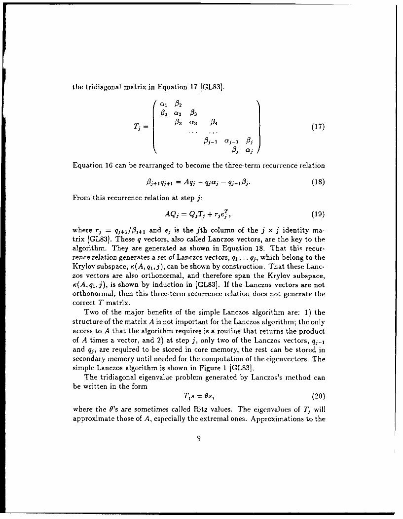
the tridiagonal matrix in Equation 17 [GL83).

032 a2 /3

Tj =3 a 3 04 (17)

#j- a,- 1 Pi,

/3, a,

Equation 16 can be rearranged to become the three-term recurrence relation

plj+lq.+, = Aqj - qja, - qj--flj. (18)

From this recurrence relation at step j:

AQj = QjTj + rje, (19)

where rj = qj+1/fi+1 and ej is the jth column of the j x j identity ma-trix [GL83]. These q vectors, also called Lanczos vectors, are the key to thealgorithm. They are generated as shown in Equation 18. That this recur-rence relation generates a set of Lanczos vectors, q, ... qj, which belong to theKrylov subspace, K (A, q1, j), can be shown by construction. That these Lanc-zos vectors are also orthonormal, and therefore span the Krylov subspace,K(A, qi,j), is shown by induction in [GL83]. If the Lanczos vectors are notorthonormal, then this three-term recurrence relation does not generate thecorrect T matrix.

Two of the major benefits of the simple Lanczos algorithm are: 1) thestructure of the matrix A is not important for the Lanczos algorithm; the onlyaccess to A that the algorithm requires is a routine that returns the productof A times a vector, and 2) at step j, only two of the Lanczos vectors, qj-1and qj, are required to be stored in core memory, the rest can be stored insecondary memory until needed for the computation of the eigenvectors. Thesimple Lanczos algorithm is shown in Figure 1 [GL83].

The tridiagonal eigenvalue problem generated by Lanczos's method canbe written in the form

Tis = Os, (20)

where the O's are sometimes called Ritz values. The eigenvalues of T willapproximate those of A, especially the extremal ones. Approximations to the

9

ro = starting vtctor

# = II ro IIqo = 0j=1

while (3, 5 0)qj= rj-1 /jct= qT Aqjrj= Aqj - ajq, - Ojqj-l

#j1= (1 rjj=j+l

Figure 1: The simple Lanczos algorithm

eigenvectors of A, called Ritz vectors, can be calculated using the equation

yi = Qjsi, (21)

where yj is the Ritz vecLor coiLesponding to s, [PNO85]. These Ritz vectorssatisfy: [NOPEJ87]

Ay, = yj= 9 4- rjs,(j). (22)

4.2 Effect of Roundoff Errors

The algorithm and equations in Subsection 4.1 hold only in exact arithmetic;they degenerate in the presence of roundoff errors, and, therefore, the Lanczosvectors can no longer be assumed to be orthonormal. When roundoff errorsare taken into account, Equation 19 becomes

AQj = QTj + rjc'+ Fj, (23)

where F is used to represent roundoff error. Then,

j1 Ay, - y2 , 1i 11_< ,+ 1F, j1, (24)

can be used to bound the error in the Ritz pair (0,, y,). The norm of F canbe bounded by n1 /2 c 11 A !'. where c is a constant based on the floating point

10

precision of the combuter, and flj. = 3j+l I si(j) [ PN0851. The bound onI! F(j) is small and can be disregarded. The most important factor thenbecomes /3i. From [Pai7l]

I yqj+ I= "00/%ii, (25)

where -y is a roundoff term approximately equal to 11 A 11. From Equation 25,the conclusion can be drawn that as Oji becomes small (and hence the errorin the Ritz pair, (0j, yi), also becomes small), the q vectors lose orthogonality[Par8O]. Equation 25 implies that convergence of a Ritz pair to an eigenpairof A results in a lack of orthogonality among the Lanczos vectors. Morespecifically, significant components of yi, the converged Ritz vector, creepinto subsequent qj's, causing spurious copies of Ritz pairs to be generated bythe Lanczcs process.

Several remedies for the loss of orthogonality have been proposed. Paigesuggests full reorthogonalization, in which the current Lanczos vector, q,, isorthogonalized against all previous Lanczos vectors [Pai7l]. Full reorthogo-nalization becomes increasingly expensive as j grows. Cullum and Willoughbyadvocate a method in which the lack of orthogonality is ignored and sophis-ticated heuristics are used to detect the eigenvalues that are being soughtamong the many spurious eigenvalues that are generated [CW85]. Simonproposes a scheme called partial reorthogonalization in which estimates forthe orthogonality of the current Lanczos vector, qj, against all previous Lanc-zos vectors are inexpensively computed. Based on the estimates, a smallset of the previous Lanczos vectors are orthogonalized against qj [Sim84].Partial reorthogonalization maintains semi-orthogonality among the Lanc-zos vectors. For all q vectors, semi-orthogonality is defined by:

qTqt<I/2 i7j. (26)

"Semi-orthogonality" among the q vectors guarantees that the T matrix gen-erated by the Lanczos algorithm executed with roundoff errors will be thesame up to working precision as the T matrix generated using exact arith-metic [PNO85]. Selective orthogonalization is used by LANZ in an adaptedform to maintain semi-orthogonality among the Lanczos vectors [PS79]. Thestrategy of selective reorthogonalization, as proposed by Parlett and Scott,orthogonalizes the current residual vector, rj, and the last Lanczos vector,qj-,, at the beginning of each step in the Lanczos algorithm against "good"

11

Ritz vectors (more details of how this occurs will be given in Section 5)."Good" Ritz vectors are those which correspond to Ritz values for whichthe value of /3 ji is below c'/2 11 A 11. A low /3ji value suggests that the Ritzvalue is converging and, therefore, from Equation 25, I Y, qj+l I is increasing.The value of fl/2 II A 11 is used to ensure that the quantity I yTqj+l I neverrises above O/2. As a result, semi-orthogonality, as defined in Equation 26,is maintained.

12

5 The LANZ Algorithm

5.1 The Spectral Transformation

In order to use Lanczos's method to find the lowest eigenvalues or the eigen-values closest to some value, a, of Kx = AMx, a transformation of theproblem must be made. The Lanczos algorithm described in Section 4 isapplicable only to Ax = Ax. Two transformations are available when K andM are symmetric and M is positive semi-definite. Each transformation inthis section will be represented by a capital letter that has no other mean-ing. Transformation A, proposed by Ericsson and Ruhe, replaces A withWT(K - aM)-'W to yield,

WT(K - aM)-'Wy = vy, (27)

where M = WW T , y- WTX, and A = a + 1/v [ER80]. Transformation B,suggested by Nour-Omid, Parlett, Ericsson and Jensen, replaces A with (K-aM)-M and uses the M-inner product, because the operator is no longersymmetric [NOPEJ87]. Note that M does not form a true inner productbecause M is not positive definite. This semi-inner product is acceptable,however, because the only situation in this algorithm in which zTMx = 0,for a non-trivial x, is when Pj+l = 0, which indicates exact convergence inthe Lanczos algorithm. (Hereafter, the semi-inner product will be referredto as just an inner product). Equation 1 becomes

(K - aM)-'Mx = vx, (28)

where the eigenvalues of the original system can be recovered via

A = (7 + 1/u. (29)

Transformation B is a shifted inverted version of Equation 1 by virtue of thefollowing steps. Substituting Equation 29 in Equation 1 yields

Kx - aMx = 1/vMx. (30)

Then, solving for x and multiplying by t/ gives

vx = (K - aM)-1 Mx. (31)

13

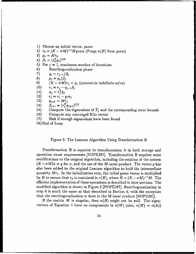
1) Choose an initial vector, guess2) ro = (K - aM)-'Mguess (Purge n(B) from guess)3) Pi = Mro4) I1 = (rojPi)' '

5) For j = 1, maximum number of iterations6) Reorthogonalization phase7) q. = r. I /88) p, = p / 89) (K - aM)ri = pj (synunetric indefinite solve)10) rr= - 111) a T

12) rj =r - q crj13) P.+l = Mrj

14) /fj+1 = (r=pj+1)1 / 2

15) Compute the eigenvalues of Ti and the corresponding error bounds16) Compute any converged Ritz vector17) Halt if enough eigenvalues have been found18) End of Loop

Figure 2: The Lanczos Algorithm Using Transformation B

Transformation B is superior to transformation A in both storage andoperation count requirements [NOPEJ87]. Transformation B requires somemodifications to the original algorithm, including the solution of the system(K - aM)x = y for x, and the use of the M-inner product. The vector p hasalso been added to the original Lanczos algorithm to hold the intermediatequantity Mri. In the initialization step, the initial guess vector is multipliedby B to ensure that r0 is contained in r(B), where B = (K -aM)-M. Theefficient implementation of these operations is described in later sections. Themodified algorithm is shown in Figure 2 [NOPEJ87]. Reorthogonalization instep 6 is much the same as that described in Section 4, with the exceptionthat the reorthogonalization is done in the M-inner product [NOPEJ87].

If the matrix M is singular, then n(B) might not be null. The eigen-vectors of Equation 1 have no components in n(M) (also, n(M) = n(B))

14

[NOPEJ87]. In exact arithmetic, if the starting vector, qo, of the Lanczosprocess is restricted to r(B), then all subsequent Lanczos vectors will be re-stricted to r(B), because they are computed by multiplying by B. However,in finite precision arithmetic, roundoff error allows components of subsequentLanczos vectors to be in n(B); therefore, the Ritz vectors calculated fromthem will have components in n(B) [NOPEJ87]. Purifying these Lanczosvectors is an expensive process, but a method exists that instead will in-expensively purify the calculated Ritz vectors. The vector wi is computed,where wi is a j + I-length vector whose first j components are calculated as,

w, = (1/0,)(Tjs,), (32)

and whose last component is

(S,(lj+1)/8,. (33)

Equation 21 then becomes:

yi = Qj+wi, (34)

where wi has replaced si.

5.2 Transformations for Buckling

Transformations A and B are not applicable to the buckling problem becauseKG can be indefinite. Transformation A fails because it requires the Choleskifactorization of KG. Transformation B fails because it requires the use of aKG-inner product which would be an indefinite inner product and introducecomplex values into the calculations. Transformation C, suggested for thebuckling problem in [Ste89b], uses the operator (K + aK) - 'K. The trans-formation (K - aKG) is actually suggested in [Ste89b], but (K + aKG) ispreferred because it yields the correct inertia for the buckling problem (notethat the inertia referred to here is not the inertia of a physical body, it isthe definition of inertia used in Sylvester's inertia theorem relating to thenumber of positive, negative, and zero eigenvalues of a matrix). The inertiaof (K + aKG) reveals how many eigenvalues of Equation 3 are less than a.Transformation C can be derived from Equation 3 by substituting orv/(v- 1)

15

for A in Equation 3, multiplying each side by (v - 1), rearranging terms, andfinally, multiplying each side by (K + oKG)- 1 to yield

vx = (K -, aK)-'Kx. (35)

To recover A, use Equation 36.

A = cV/(v - 1). (36)

Transformation C requires that a be non-zero. The factorization of (K +aKG) and the use of the K-inner product are necessary for transformationC.

In exact arithmetic, the convergence rate of the Lanczos algorithm is thesame for transformations B and C when a is fixed (B performs the sametransformation on the spectrum as A). The Kaniel-Page-Saad theory is usedto explain the convergence of eigenvalues when using the Lanczos algorithmand is now introduced to allow a comparison of the transformations andto show the effects of moving a on the convergence rate [Saa8O]. Threedefinitions that will be useful in this explanation are:

i-I

Ki' = 1- (0' - vf)/(v, - vi), (37)M=1

"yj = 1 + 2(vi - vi+ , )/(v+ 1 - v1,f), (38)

and the Chebyshev polynomial,

C.(x) = l/2((x + (x2 - 1)1/ 2 )n + (X - (X2 - 1)1/2)n). (39)

The bound on the difference between an eigenvalue of the Tj matrix, 0,, andan eigenvalue of the transformed system, vi, at the jth step of the Lanczosalgorithm is

0 < vi - 04 < (vi - vinf)(Kitan w(xj,ro)/Cj_i(-y,))2 , vi > vi+,. (40)

The tan w(x,, ro) is determined by the angle between the eigenvector, xi,associated with V, and the starting Lanczos vector, r0 . Because the angle be-tween xi and r0 does not change during the Lanczos algorithm and becauseK does not vary greatly, the term that governs the rate of the convergenceis Cij(-t). As j increases, Ciji(-yi) grows more quickly for large Oi than for

16

Eigenvalue order o =0 a=10 a=25 a=25.9

26 A, 0.2199 0.3214 4.2857 42.344230 A2 - - -

100 A, I - - I-

Figure 3: Effects of transformation on eigenvalue separation

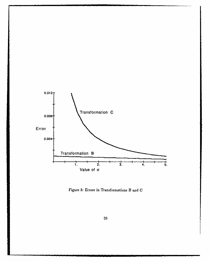
small qOi (0i is a term, I(vi-v+1 )/(v+l-j,) - , obtained from the definitionof -y). The €j reflect the separation of individual eigenvalues from their neigh-bors relative to the remaining width of the spectrum. Transformations areused to increase gi for the desired eigenvalues by transforming the spectrumsuch that the desired eigenvalues are well-separated from other eigenvalues.It can be shown that, if used with the same a, transformations B and C havethe same effect on the 4i. However, moving a closer to a desired eigenvalue,A,, increases the corresponding Oi (and therefore speeds convergence of 01 toA1). The increase in qj as a is moved closer to A, is shown in Figure 3. Thus,as a is moved closer to A, the convergence of 01 to A, is speeded up.

Transformations B and C have the same effect on the convergence ratesof the Lanczos process and C can be used in both the buckling and vibrationproblems, so the question arises "Why not use transformation C for both thebuckling and vibration problems?" Although B and C have the same effectin exact arithmetic, they each yield different v's for the same a. In finiteprecision arithmetic, transformation C is inferior to transformation B whena is small relative to the desired A's. Although each transformation requiresthe solution of a linear system and the multiplication of a matrix by a vector,the distribution of the v's for small a in transformation C leads to largeerrors in the computation of the A's. For small a, the v's of transformationC become close to 1 while the same effect is not seen when transformationB is used (note that the Oi's in each case are identical). The v's that resultwhen using transformation C become increasingly close to 1 as a is movedfrom 1.0 to 0.01, whereas the v's that result when using transformation Bshow little change (this trend is shown in Figure 4). Because the Lanczosalgorithm consists of the same calculations for each transformation, in finiteprecision arithmetic the algorithm computes perturbed values asbumcd to be

17

Eigen- order a = 1.0 a = 1.0 or = 0.01 a=0.01value v for v for v for v for

Trans. B Trans. C Trans. B Trans. C26 A, 0.04000 1.04000 0.03848 1.0003848

26 A, 0.04000 1.04000 0.03848 1.000384830 A2 0.03448 1.03448 0.03334 1.0003334100 A, 0.01010 1.01010 0.01000 1.0001000

Figure 4: Effects of transformation on eigenvalues

of the form, (1 + c)v, instead of an exact v. The effect of this perturbation onthe computed A's is the difference between the two transformations. Recallthat in transformation B, A = a + 1/vB, and that in transformation C,A = a + a/(vc - 1) (the subscript on v is introduced because the v's aredifferent in each transformation and these values are being compared). If vcis solved for in terms of vB, then

VC = aVB + 1. (41)

Let 6 AB and bAC denote the difference between the true A and the A computedusing transformations B and C, respectively. These 5A'- ar. cpressed interms of perturbed v's in the following equations:

A+ AB = O + 1/(1 + )VB, (42)

A + bAc = a + a((1 + c)vc -1). (43)

If Equation 41 is substituted into Equation 43, then

A + bAc = U + al(a B + oCVB + E). (44)

If the true A is subtracted from each side of Equations 42 and 44, then

6AB = 1I(VB + fVB) - 1/IB. (45)

6Ac = 1I(VB + (:VB + c/a) - 1/VB. (46)

Thus, the error in the computed A for transformation C increases sharplyas a decreases. To show the increase in error for transformation C, the

18

errors in the two transformations (from Equations 45 and 46) are plotted inFigure 5 for A = 10 and e = 0.0001. From this derivation and the graph ofthe functions, it is clear that transformation C should be avoided when a issmall compared to the desired A.

From the previous discussion the conclusion can be drawn that trans-formation B is preferred to C whenever possible. However, as was pointedout previously, transformation B is not applicable to the buckling problom.Therefore, a new transformation, D, which transforms the eigenvalues in thesame fashion as transformation B (when or = 0) is introduced. Transforma-tion D can be used with an indefinite KG matrix but can only be used whena is 0. Transformation D is derived from Equation 3 in the following steps[CW85]: first, substitute 1/v for A and then multiply each side by K-1v toyield

vx = K - Kx; (47)

next, expand the implicit identity matrix in each side as I = C-TCT, whereK = CCT, let y = CTx, and, finally, multiply each side by CT to y;,Id

vy = C- 1 KGC-Ty. (48)

The operator for transformation D is C-KGC-T. This transformation re-quires the Choleski factorization of K and uses the standard inner product.

The eigenvectors, x, must be recovered via the solution of a triangular linearsystem, using the foregoing equation for computing y. When an initial non-zero guess for a exists, the method used in LANZ for solving the bucklingproblem uses transformation C exclusively; when an initial guess for a isn'tavailable, the method used begins by using transformation D with a at 0,and then switches to transformation C when a shift of a is needed (the useof shifting will be described in the next subsection). Thus, the use of trans-formation C with small a is avoided, and, yet, the advantage resulting fromshifting is maintained.

5.3 The Use of Shifts

An efficient algorithm for computing several eigenva]ues requires that theshift, a, be moved as close as possible to the eigenvalues that are being com-

puted. The closer that a is to an eigenvalue being computed, the faster theconvergence to that eigenvalue. Ericcson and Ruhe describe a method for

19

0.012"

Transformation C0.008

Error

0.004"

Transformation B

1. 2. 3. 4. 5.

Value of a

Figure 5: Errors in Transformations B and C

20

selecting shifts and deciding how many Lanczos steps to take at each shift[ER80]. The efficiency of the algorithm depends on how well these shifts arechosen, and how many Lanczos steps are taken at each shift. Normally, themost expensive step in the Lanczos process is the factorization of (K - 0,M),which must be done once for each shift. But if j becomes large, the calcu-lation of an eigenvector, Equation 21, caii be very expensive. In addition,many steps could be required to converge to an eigenvalue if the shift is faraway from this eigenvalue, or if the eigenvalue is poorly separated from itsneighbors. The method used by Ericcson and Ruhe first estimates that reigenvalues will converge in j steps, where r is calculated based on the factthat the eigenvalues of Equation 1 are linearly distributed. A cost analysis ofthe algorithm is performed, and from this analysis, a determination of howmany steps to take at a shift is made. Their choice of shift depends on theinertia calculation in the factorization step [ER80].

In the problems from the NASA structures testbed [Ste89a], the distribu-tion of the eigenvalues is often anything but linear. This distribution makesthe above estimates invalid and requires a different method for deciding howmany steps to take at each shift. Instead of calculating the number of stepsto take for a shift prior to execution, LANZ uses a dynamic criterion todecide when to stop working on a shift. Later, in Section 6, a cost analy-sis of the Lanczos algorithm shown in Figure 2 is given. This cost analysisis part of the basis for the dynamic shifting algorithm. The implementa-tion of LANZ, however, uses execution timings, rather than a precalculatedcost analysis, because the cost analysis is different for each architecture onwhich the implementation is run. These timings let LANZ know how longeach Lanczos step takes and the cost of factorization at a new shift. Inaddition to the timing information, the estimated number of steps requiredfor unconverged eigenvalues to converge is calculated. The step estimateis computed by tracking the eigenvalues of T (and the corresponding errorbounds) throughout the execution of the Lanczos algorithm. The method forthis tracking and computation of eigenvalues is described in Section 7. Withestimates for the number of steps required for eigenvalues to converge andthe time needed for a step (or new factorization) to execute, the decision tokeep working on a shift or choose a new shift can be made efficiently.

The selection of a new shift depends on the information generated dur-ing the execution of LANZ on previous shifts and on inertia calculations atprevious shifts. The inertia calculations are used to identify any eigenvalues

21

that were skipped over in previous steps, including eigenvalues of multiplicitygreater than one. The estimated eigenvalues and their error bounds gener-ated during the execution of Lanczos enable the selection of a new shift basedon these estimates (if no eigenvalues were skipped in the previous run). Be-cause convergence to an eigenvalue is faster if the shift, a, is chosen to beclose to that eigenvalue, LANZ seeks to choose a shift that is near to thedesired unconverged eigenvalue. However, a must not be chosen so close toan eigenvalue that the system (K - aM)x = y becomes very ill-conditioned.In the authors' experience, Lanczos's method generates approximations toall nearby eigenvalues, so that even if an eigenvalue is not converged to, anestimate along with an error bound for a nearby eigenvalue is generated. Ifthe initial Lanczos vector is not deficient in the eigenvector correspondingto an eigenvalue, and if that eigenvalue is close to o,, then the Kaniel-Page-Saad theory shows that Lanczos's method will generate an estimate to thateigenvalue in a few steps [Kan66]. In practice, even if the initial Lanczosvector is deficient in the eigenvector, round-off error will quickly make thateigenvector a component of the Lanczos vectors [ER80].

When a new shift is chosen, the initial Lanczos vector is chosen to bea weighted linear combination of the Ritz vectors corresponding to the un-converged Ritz values of the previous shift, where the weights are chosen asthe inverse of the error bounds of those Ritz values [PS79]. The number ofRitz vectors chosen is based on the number of eigenvectors still to be foundand the number of Ritz vectors with "reasonable" error bounds. To exam-ine the effect of using a linear combination of Ritz vectors rather than arandom vector as the initial vector, several structural engineering problems(both buckling and vibration) were solved using both methods for selectingan initial vector (for an explanation of the problems used, see Section 9). Thenumber of steps taken by each method to get the same number of eigenvaluesis given in Figure 6 and from this it appears that using the linear combinationof Ritz vectors is always as good or better than choosing a random vector.

To give the reader a clearer picture of the overall execution flow of LANZ,a flow chart is shown in Figure 7.

5.4 Selective Orthogonalization

The method used to maintain "semi-orthogonality' among the Lanczos vec-tors is a modification of selective orthogonalization as proposed by Parlett

22

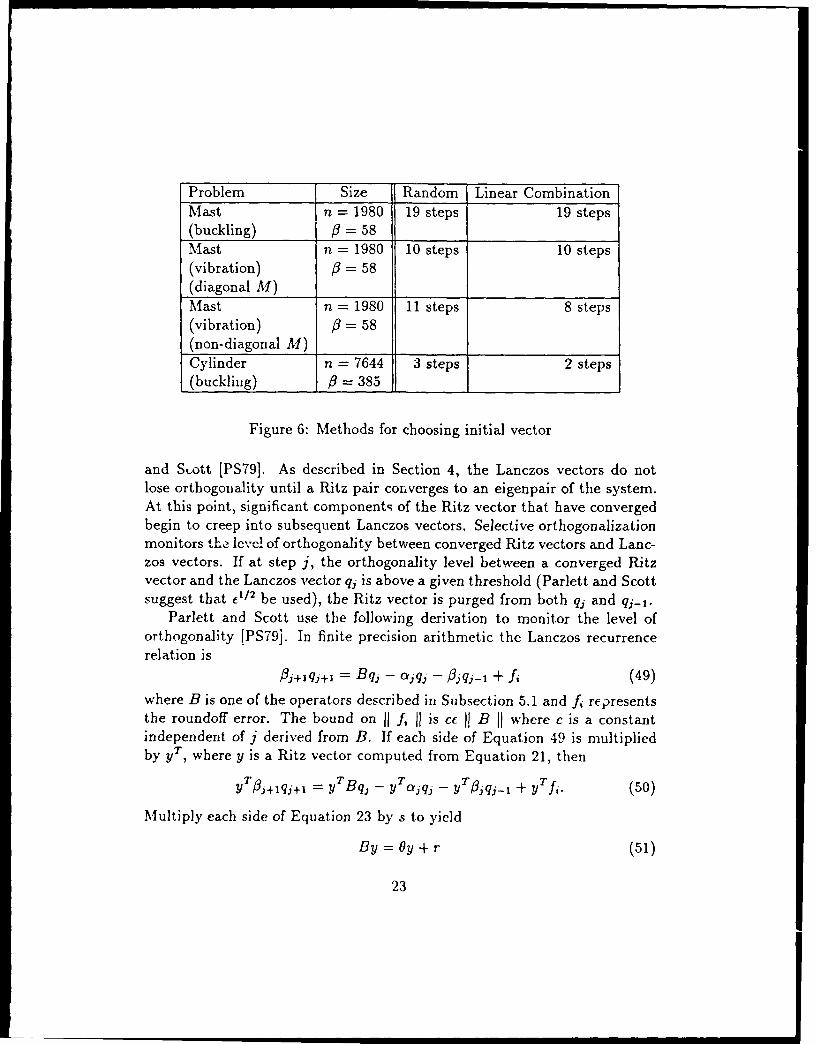
Problem Size Random Linear CombinationMast n = 1980 19 steps 19 steps(buckling) = 58Mast n = 1980 10 steps 10 steps(vibration) = 58(diagonal M)Mast n = 1980 11 steps 8 steps(vibration) = 58(non-diagonal M)Cylinder n = 7644 3 steps 2 steps(buckliug) /3 = 385

Figure 6: Methods for choosing initial vector

and Scott [PS79]. As described in Section 4, the Lanczos vectors do notlose orthogonality until a Ritz pair converges to an eigenpair of the system.At this point, significant components of the Ritz vector that have convergedbegin to creep into subsequent Lanczos vectors. Selective orthogonalizationmonitors the level of orthogonality between converged Ritz vectors and Lanc-zos vectors. If at step j, the orthogonality level between a converged Ritzvector and the Lanczos vector qj is above a given threshold (Parlett and Scottsuggest that c1/2 be used), the Ritz vector is purged from both qj and qi-j.

Parlett and Scott use the following derivation to monitor the level oforthogonality [PS79]. In finite precision arithmetic the Lanczos recurrencerelation is

oj+lq.+, = Bq - aq, - Ijqj_ + f, (49)where B is one of the operators described in Subsection 5.1 and f, representsthe roundoff error. The bound on 11 f; 11 is cc 11B 11 where c is a constantindependent of j derived from B. If each side of Equation 49 is multipliedby yT, where y is a Ritz vector computed from Equation 21, then

y Tpj+lqj+l = yTBq, - yTaiq,i - yT/3jqjl + yTf,. (50)

Multiply each side of Equation 23 by s to yield

By = Oy + r (51)

23

Start with the user's initial shiftor use 0 if none is specified

Execute the Lanczos algorithm until1) The desired number of eigenvalues are found,

2) No storage space is left, or3) LANZ determines a new shift is needed

(2) or (3) (1)

LANZ examines the convergedLANZ selects a new shift based and unconverged eigenvalueson accumulated information along with the inertia counts

to ensure that no eigenvalues~have been missed.

Not Okay __Okay

Finished

Figure 7: Execution flow of LANZ

24

where r is not rj and will be discussed below. If the bound for 11 f; I1 andEquation 51 are substituted into Equation 50, Equation 52 results.

3j+IYT qj+, = (OYT + J 0 3 yT)qj _ gjyTq_, + CC 11 B II (52)

Parlett and Scott assume that r = qk+I/3 ki for some k < j, and therefore,that

I qj 1< Oki I q+ 1 q3 I. (53)They then state: 1) I q ,+1q 1< /, because semi-orthogonality among the

Lanczos vectors is maintained, and 2) if y is a converged Ritz vector, then6Pj is less than or equal to fl/2 11 B 11. Fact 2 is caused by the definition

of a "good" Lanczos vector given in Section 4. If facts 1 and 2, along with7j =1 yTqj 1, are substituted into Equation 52, then Equation 54 :s derived.

-j+, < (1 0 - cj I ri +/3jTj.I+ )I B )) +cc )I B II)/,3j+l (54)

Because c and B 11 are small and not readily available, Parlett and Scottignore these terms and derive the following recurrence relation for 7j+,:

rj+l < (1 0 - ai I Tj + / ,)/ 3 +,. (55)

The values r0 and rl are initialized to c and whenever y is purged from qi,-rj is reset to f. From this recurrence relation, the conclusion can be drawnthat the Lanczos vectors should be orthogonalized in pairs.

This recurrence relation predicts the actual level of orthogonality very wellin practice with two exceptions. The first problem occurs when calculating,rj+l after y has been computed at step j - 1 and purged from qi, and qj. Inthis situation, a small increase in rj+l over Ti and rj-1 is expected. However,a large increase occurs. This increase is caused by the assumption on Parlettand Scott's part that I q',qj j< 0/2, when in fact that equation only holdswhen k < -. The quantity, I q'+qj J, is 1 when k = 3-1. Thus,Equation 55 holds when k < j - 1, but when k = I - 1 Equation 55 becomes:

rs+, < (I 0 - aj I r, + j/rj-1 + i-,.,)/3+,. (56)

The second problem arises when using Equation 34 to compute y. In thiscase r = Oy + .%-1,1qj + flj-%,Bq/0 assuming y is computed at step j - 1;therefore,

I r qj 1 o0rj + _-,, i1 ,4 ., 1a'/. (57)

25

The recurrence relation used for rj+l then becomes:

Tj,+l : (I 0 - C'j I 7j + fjTj_ 1 +e j-,i + Ij-l,itajlo)lflj+l (58)

If y has been computed at step j - 2, then

I rJqi 1 + _ 07 + /_ 2+ _2.,8j±o, (59)

and, because the second term is very small, the recurrence relation for rj+lbecomes

TJ+1 -< (I - aj I Tj + ljri + flj_ 2,,flj/o)/flj+1 . (60)

5.5 Orthogonalization Methods

Selective orthogonalization and partial reorthogonalization are the two bestknown orthogonalization methods other than full reorthogonalization. Par-tial reorthogonalization monitors the orthogonality of qi and q,+, versus theother Lanczos vectors. Partial orthogonalization measures the ortlhogonalitybetween qi and qk, Wjk, via the recurrence relation dcfined in the followingset of equations [Sim84]:

Wkk=I for k =,...,j, (61)Wkk-1 = qqk-1 for k =2,...,j, (62)

j+lWj+l+k = fj+lWjk+l + (ak - aj)wjk + / 3kWjk-1-%jIj- + q fk- qT fj (63)andWjk+l = Wk+lj for 1 < k < j. (64)

Simon has stated that the theoretical relationship between partial reorthogo-nalization and selective orthogonalization is not known [Sim84I. The follow-ing discussion explains the relationship between the two methods. If y7 onthe left side of Equation 50 is expanded to sTQT, and the resulting equationis divided by /3j+,, the right side becomes rj+,i, yielding

=T - T (65)Si tj qj+l -- Tj+l'i (5

From the recurrence relation for partial reorthogonalization, the productQT qj+ is the vector Wj+l,k, where k runs from 1 to j. Thus the relation-ship between the w's and the 7's is governed by

ST=j+l,k = Tj+l,k, wherc k = 1,...,j. (66)

26

This relationship in Equation 66 has also been observed in numerical exper-iments run by the authors. When a Ritz vector, yi, is purged from qj+l andtherefore rj+i,i becomes small, the Wj+l,k's for which the values of si,k are thelargest decrease significantly.

27

6 Execution-Time Cost Analysis

An analysis of the execution-time cost of the Lanczos algorithm when usingtransformation B is given in Appendix A. Because the costs for the othertransformations are almost identical their cost will not be analyzed in thissection. The analysis has two purposes: 1) to allow the computation of thetradeoff point between re-starting the Lanczos algorithm at a different shiftand continuing with the current shift, and, 2) to allow analysis of performanceon parallel and vector/parallel machines. Throughout the analysis, only thecost of floating point operations is included. The assumption is made forthis analysis that the matrices have a band structure and that the Bunch-Kaufman method (or an LDLT decomposition) is used for the solution ofthe linear systems. In order to simplify the analysis, the assumption is madethat the bandwidth of K is greater than or equal to the bandwidth of M. Thisassumption has no effect on the analysis other than to avoid making some ofthe operation costs conditional on which matrix has the larger bandwidth.Much of this analysis does not take into account "end conditions," such asthose that arise near the end of a factorization when less work needs to bedone than in the middle of a factorization. Thus, some of the expressions arenecessarily approximations.

Several observations regarding the shift tradeoff can be made from thecost analysis: 1) the single most expensive step in the algorithm is the fac-torization phase (2B) which is O(np2), 2) the cost of the reorthogonalizationphase increases as j increases because of the increasing number of "good"Ritz vectors to orthogonalize against, 3) the cost of computing a convergedRitz vector is based on j 2 and therefore increases rapidly as j increases, and4) the cost of the rest of the operations in the program loop is not affected bygrowth in j (with exception of step 15 but this step is not costly enough toconsider). To illustrate how the costs of the four operation groups per Lanc-zos step change, the number of floating point operations per step is plottedagainst j, the number of Lanczos steps, in Figure 8. The costs in the Fig-ure 8 are from an actual LANZ run during which a new shift was selectedbeginning at step 22. These costs, of course, will differ for each problem.From the cost analysis and this graph it can be seen that a tradeoff existsbetween the benefits of a taking a new shift (smaller reorthogonalization andeigenvector computation cost as well as accelerated convergence to desiredeigenvalues) and the benefit of continuing work on the current shift (avoiding

28

4,000,000

3,000,000

FLOPS

2,000,000Factorization

1,000,000

Lanczos Step Cost

I itz Vector Compuittl Reorth gonalization

04 8 12 16 20 24 28 32

Lanczos Step Number

Figure 8: Operation costs plotted against Lanczos step number

the cost of refactorization).The LANZ implementation uses actual timings of the various steps dur-

ing the current run to analyze the tradeoff, rather than substituting valuesfor the cost of various operations for the machine being used. The use oftimings is simpler to implement and makes the code more portable.

29

.... ........... . . . . . .= = I = 1 I I I II I

7 Solution of the system Ts = Os

The size, j, of the tridiagonal system, Ts = Os, generated by the Lanczosalgorithm is 1 at step 1 and increases by 1 at each Lanczos step. The sizeof T is usually very small compared to the size of the original problem, n.Therefore, the time used to solve the tridiagonal system does not greatlyaffect the sequential execution time of the LANZ algorithm. However, if therest of the algorithm is parallelized, the solution of the tridiagonal systemcould well become a large factor in the parallel execution time. Parlettand Nour-Omid have proposed a method of tracking a small group of theeigenvalues of the T matrices as they are produced by the Lanczos algorithm.An inexpensive by-product of their method is the error bounds for the Oi's[PN085). Their algorithm monitors the outermost O's whose error bounds,Ilji, indicate that they will converge in the next 2 or 3 steps; it actuallymonitors 8 eigenvalues at a time. There are two phases: 1) the previousO's and their error bounds are updated and any new O's are detected, and2) converged O's are detected and removed from the data structure. Thisalgorithm is not suitable for use by LANZ for 3 reasons: 1) it is not easilypar, Ilelizable, 2) it does not track an eigenvalue for many steps to get aconvergence rate estimate, and 3) in tests run by the authors, it often failed.

The authors have developed a new solution method that is: 1) inherentlyparallel, 2) tracks all the eigenvalues of T from step to step, and 3) has beenused successfully with LANZ to solve real structures problems. The methoduses information from step j- 1 to solve for all the eigenvalues and their errorbounds at step j. It uses Cauchy's interlace theorem, shown in Equation 67,to find ranges for the all the eigenvalues (except the outermost eigenvalues)of Tj from the eigenvalues of Tj-,.

Oil' < 60 < Oj+ ' < Oj... jj+' < 0" < 0, + ' (67)

Cauchy's interlace theorem states that the eigenvalues of Ti interlace thoseof Ti+l [Par80]. In addition to the interlace property, the error bounds, /ji,from the previous step can be used to provide even smaller ranges for someeigenvalues. If good error bounds, fjj, are not available for the outer eigenval-ues (the interlace property only gives a starting point for these eigenvalues),they can be found by extending an interval from the previous extreme eigen-value. However, a property of the Lanczos algorithm is that the extreme

30

eigenvalues are usually the first to stabilize. The algorithm for the methodjust described is given in Figure 9. For simplicity, the algorithm does notshow the code for handling extreme eigenvalues. The algorithm requires twosubroutines, the root finder described below and a function, numless, thatuses spectrum slicing to determine the number of eigenvalues of Tj less thana value. Details of how to efficiently implement these subroutines are givenby Parlett and Nour-Omid [PN085].

A root finding method, such as bisection or Newton's method, can beused to find the eigenvalues in the ranges given by the algorithm in Figure 9[PN085]. Newton's method is preferred for its fast convergence and becauseit generates the jth element in s, as a by-product, which allows for the inex-pensive computation of the error bound for Oi [PN085]. For safety's sake, theNewton root finder is protected by a bisection root finder to ensure that New-ton's method converges to the desired root. If the Ritz vector correspondingto a particular eigenvalue, Oi, needs to be computed, inverse iteration can beused to compute si. Because the calculation of every eigenvalue is indepen-dent, this algorithm is inherently parallel. In order to save time, it may bebeneficial to keep track of which eigenvalues of T have stabilized, as these donot need to be recomputed. The major difficulty in parallelizing this algo-rithm appears to be load balancing; it will take different numbers of Newtoniterations to find each eigenvalue, and only occasionally will inverse iterationbe necessary.

The algorithm developed by the authors for solving the tridiagonal systemalso tracks the eigenvalues of T from step to step. This tracking is necessaryfor two reasons. First, selective orthogonalization requires the computation ofthe Ritz vectors corresponding to the eigenvalues of Ti that become "good"(as defined in Section 4) at step j. Those Ritz vectors can be used fromstep j + 1 until the end of the Lanczos run if the eigenvalues in T+ 1 (andsubsequent Ti's) that correspond to the eigenvalues in T can be identified.Second, the rate of convergence of a particular eigenvalue is predicted bytracking its convergence over several steps (the use of the convergence ratewas described in a previous section).

31

bounded[i] 0 , for i = 1, jdo i = 1, j -1

if ((2*#ii <D8i - Oi-1) and (2*fli, < Oi+I - Oj)) thenprobe = 0, + filess = numless(probe)if (less = i) then

bounded Ii] = ielse 1* i and i + 1 are the only values numless will return, if

it returns something else, a grave error has occurred *bounded[i + 1] = i

endifendif

enddodo i = 1, j

if (boundedlil = 0) thenleftbound = Oj-1

rightbound = 0,newtonroot(leftbound,rightbound,newO, ,newfij,)

else if (bound[i] = i) thenleftbound = 0, - iriglitbound = 0,newtonroot(leftbound,rightbound,new0, ,new3 11 )

else if (bound[i] = i - 1) thenleftbound = O-rightbound = Oi-I + /Jji-1

newtonroot (leftbound ,rightbound,new0, ,newpi3~)endif

enddo

Figure 9: Tridiagonal Eigenvalue Solver

32

8 The Solution of the system (K - aM)x = y

The solution to the possibly indefinite system,

(K - aM)x = y, (68)

is normally the most time-consuming step in the Lanczos algorithm for trans-formations A, B, and C (unless there are very few non-zero elements in(K - aM)). Therefore, it makes sense to try to optimize this step of thealgorithm as much as possible. Two approaches can be taken to solvingthis system: 1) the use of direct solution methods, or 2) the use of iterativesolution methods. Because the problems under consideration can be veryill-conditioned, the use of iterative methods has been avoided.

Because this paper is focused on the problem in which K and M arebanded, the discussion in this section is limited to the banded case. In thevibration problem, because K is positive definite and M is semi-positivedefinite, if a < 0, then the system in Equation 68 is positive definite. In thebuckling problem, because K is positive definite, if a = 0, then only K mustbe factored because transformation D is used. Because K and M are alwayssymmetric, Choleski's method can be used to solve these systems. Choleski'smethod is the direct method of choice for this class of banded linear systemsbecause it is stable and results in no destruction of the bandwidth [BKP76].Choleski's method is used by LANZ for the vibration problem whenevercr < 0 and in the buckling problem whenever a = 0.

The system in Equation 68 can be indefinite whenever a > 0 in thevibration problem and may be indefinite in the buckling problem when ais non-zero. When the system is indefinite, Choleski factorization will failbecause a square root of a negative number will be taken, and the LDLTdecomposition is not stable because the growth of elements in L cannot bebounded a priori [Wil65]. The methods of choice for factoring a full symmet-ric indefinite matrix are the Bunch-Kaufman method and Aasen's method[BG76]. It was believed that both methods, however, would destroy thestructure of a banded system and not be competitive with Gaussian elimi-nation with partial pivoting, which does not destroy the band structure butignores symmetry [BK771. To address this, the authors have developed anew method of implementing the Bunch-Kaufman algorithm which is themethod of choice for factoring symmetric indefinite banded systems when

33

the systems have only a few negative eigenvalues [JP89]. This is exactly thecase which arises when moving the shift in search of the lowest eigenvaluesof Equation 1 in the vibration problem and is often the case in the bucklingproblem as well. The modified algorithm takes full advantage of the sym-metry of the system, unlike Gaussian elimination, and is therefore faster toexecute and takes less storage space. LANZ uses this algorithm wheneverthe system can be indefinite. As an additional benefit, the inertia of thesystem can be obtained virtually for free [BK77].

Regardless of which factorization method is used, the system is only fac-tored once for each a. After the factorization has taken place, each timethe solution to Equation 68 is required, only back and forward triangularsolutions (and a diagonal solution in the Bunch-Kaufman case) must be ex-ecuted.

34

9 Performance Analysis

9.1 Vectorization

From the analysis in Appendix A it appears that vectorizing LANZ would:czult in sg:nificant speedup of the solut.'n procedure. The LANZ codewas compiled using the Convex Vectorizing Fortran compiler [Cor87]. Thecode was executed using double precision on a Convex 220 in both vectorand scalar modes. Seven free vibration problems and five buckling problemsof varying sizes from the NASA Langley testbed were run. The problemsconsisted of varying sizes of three different structures. The first structure is athin circular, cylindrical shell simply supported along its edges. The bucklingeigenvalues for this structure are closely spaced and present a challenge foreigensolvers. The actual finite element model only needs to model a smallrectangle of the cylinder to correctly simulate the behavior of the structure.A plot of the entire cylinder that shows the 15 degree rectangle of the cylinderthat is modeled is given Figure 20 of Appendix A. The two lowest bucklingmodes for an axially-compressed cylinder are are also plotted in Figure 21 ofAppendix A. The second structure is a composite (graphite-epoxy) blade-stiffened panel with a discontinuous center stiffener. The finite element modelfor this structure is shown in Figure 22 of Appendix A. The third structure isa model of a deployable space mast constructed at NASA Langley ResearchCenter. A picture of the deployable mast along with a plot of the finiteelement model is shown in Figure 23 of Appendix A. Descriptions of the firsttwo structures can be found in [Ste89a]. A description of the deployable mastcan be found in [HWHB86]. In every problem, at least ten eigenpairs werefound. All times in this section are given in seconds. In each problem, n willrefer to the number of equations, and / will refer to the semi-bandwidth ofthe K matrix. The execution times for the vibration problem with a diagonalmass matrix are given in Figure 10 where a speedup due to vectorization ofup to 7.83 is shown. Speedups of up to 7.30 for the vibration problem witha consistent mass matrix are given in Figure 11. For the buckling problem,speedups of up to 7.79 can be observed in Figure 12. These speedups aresimilar to the speedups obtained by other linear algebra applications on theConvex 220. From these comparisons the conclusion can be drawn thatsignificant speedup of the solution procedures due to vectorization can beachieved.

35

Problem Size Vector Scalar Speedup(seconds) (seconds) Factor

Mast n - 1980 2.80 9.28 3.31# =58 _

Cylinder n = 16 0.40 0.92 2.303=65

Cylinder n = 1824 3.64 20.42 5.61# = 185

Cylinder n = 7644 34.77 256.47 7.38# = 385

Cylinder n = 12054 75.79 593.48 7.83#_= 485

Panel n = 477 1.04 3.69 3.55# = 142 1_1

Panel n = 2193 6.04 35.49 5.88_ _ = 237

Figure 10: Vectorization Results for the Vibration Problem with a DiagonalMass Matrix

36

Problem Size Vector Scalar SpeedupI (seconds) (seconds) Factor

Mast n = 1980 4.05 10.52 2.603= 58

Cylinder n = 216 0.44 0.96 2.18/3 = 65

Cylinder n = 1824 4.69 22.12 4.723 = 185

Cylinder n = 7644 39.26 263.73 6.723 = 385

Cylinder n = 12054 82.88 605.30 7.30_3 = 485

Panel n = 477 1.74 5.18 2.98S3 = 142 1 1 1

Panel n = 2193 10.61 43.82 4.133 = 237

Figure 11: Vectorization Results for the Vibration Problem with a ConsistentMass Matrix

Problem Size Vector Scalar Speedup(seconds) (secnds) Factor

Mast n = 1980 5.16 14.72 2.85,8 = 58

Cylinder n = 216 0.43 1.01 2.353 =65 1

Cylinder n - 1824 5.18 27.54 5.32/3 = 185

Cylinder n - 7644 70.32 510.75 7.26/3 = 385

Cylinder n = 12054 10.57 1172.39 7.79_ _ = 485 _ __

Figure 12: Vectorization Results for the Buckling Problem

37

9.2 Comparison With Subspace Iteration

The claim was made in Section 3 that Lanczos's method is significantly fasterthan subspace iteration. The results presented in this section support thisclaim. The LANZ code was compared with the EIG2 processor from theNASA Langley testbed code. The EIG2 processor uses the subspace itera-tion method [Ste89b]. Both codes were compiled and executed as in Sub-section 9.1. The same problems that were solved in 9.1 were used for thiscomparison in which the the lowest ten eigenvalues were sought. Both pro-grams were able to find the lowest ten eigenvalues in every case, althoughEIG2 took an unusually large number of iterations (over three times the rec-ommended maximum) to find them in the Mast case for both the bucklingand free vibration problems. The Mast problem has a difficult distributionof eigenvalues, and the LANZ code makes use of shifting to quickly find theeigenvaiues. Both codes were directed to find the eigenvalues to a relativeaccuracy of 10 - . However, the subspace iteration code used an accuracymeasure which was more lax than that used in the LANZ code. The mea-sure used in the subspace code,

(Ak+1 _ k)/A k+1 (69)

where k is the iteration number, is only a check to determine whether aneigenvalue has stabilized relative to itself. In the LANZ code

(11 Ky - OMyj II) 1 , (70)

is used to check the relative accuracy of the combination of the eigetivalueand the eigenvector. Therefore, the LANZ code is at a disadvantage to thesubspace code in this comparison because the eigenpairs are computed togreater accuracy than in the subspace iteration code.

When the results comparing the two codes are given, two times are re-ported for LANZ: the processing time required by the code and the totalof the system and processing time required by the code. The two times aregiven because the EIG2 processor can only report its execution time as thetotal of system and processing time. For the free vibration problem witha diagonal mass matrix, LANZ is shown in Figure 13 to be about 7 to 14times faster than subspace iteration. In Figure 14, LANZ is shown to beabout 7 to 26 times faster than subspace iteration for the vibration problem

38

Problem Size LANZ LANZ Subspace Iteration RatioProgram Total Total

(seconds) (seconds) (seconds)Mast n = 1980 2.80 2.85 29.40 10.32

13 = 58Cylinder n = 216 0.40 0.41 5.70 13.9013 = 65Cylinder n = 1824 3.64 3.73 46.40 12.44

t= 185Cylinder n = 7644 34.77 35.18 313.80 8.92

S =385Cylinder n = 12054 75.79 76.65 541.50 7.06

)3 = 485Panel n = 477 1.04 1.07 12.30 11.50

03 = 142

Panel n = 2193 6.04 6.17 82.30 13.34-P 237 1 1

Figure 13: LANZ vs. Subspace Iteration: Vibration Problem with DiagonalMass Matrix

39

Problem Size LANZ LANZ Subspace Iteration RatioProgram Total Total

(seconds) (seconds) (seconds)Mast n = 1980 4.05 4.08 107.60 26.37

/=58Cylinder n = 216 0.44 0.44 5.90 13.41

/3=65Cylinder n = 1824 4.69 4.77 51.60 10.82

/3 = 185Cylinder n = 7644 39.26 39.74 357.10 8.99

/= 385Cylinder n = 12054 82.88 83.80 585.10 6.98

/3=485Panel n = 477 1.74 1.77 20.50 11.58

# = 142 1Panel n = 2193 10.61 10.72 109.80 10.24

/3 = 237 1 1 _1 _

Figure 14: LANZ vs. Subspace Iteration: Vibration Problem with Consis-tent Mass Matrix

40

Problem Size LANZ LANZ Subspace Iteration RatioProgram Total Total

(seconds) (seconds) (seconds)Mast n = 1980 5.16 5.22 108.9C 20.86

_ = 58Cylinder n = 216 0.43 0.44 5.60 12.73

_ = 65Cylinder n = 1824 5.18 5.30 92.80 17.51

= 185Cylinder n = 7644 70.32 70.84 523.90 7.40

# = 385 1 1 1Cylinder n - 12054 150.57 151.44 992.30 6.55

8 = 485 _

Figure 15: LANZ vs. Subspace Iteration: Buckling Problem

with a consistent mass matrix. LANZ is shown to be about 6 to 21 timesfaster than subspace iteration for the buckling problem in Figure 15.

LANZ's advantage over subspace iteration appears to be diminishing asthe problem sizes increase because the factorization of the matrices takes alarger proportion of the time as the matrix size increases. Because each codecould use the same factorization technique, the time spent in factorizationdistorts the advantage that LANZ holds over subspace iteration. To moreclearly illustrate the advantage of LANZ over subspace iteration, the timefor factorizing (K - aM) was removed from the results in Figures 13, 14,and 15. Only the totals of system and processing time were accessible whencomputing the modified times. Although the time for triangular linear sys-tem solutions (the backward, forward, and diagonal linear solutions requiredat each step) is still included, the modified times will give the reader a bet-ter comparison of the time spent in the eigensolving routines. In Figure 16,LANZ now shows an advantage of up to 47.18 for the vibration problem witha diagonal mass matrix. For the vibration problem with a consistent massmatrix, a speedup of up to 31.31 can be observed in Figure 17. A speedupfor the buckling problem of up to 23.64 is shown in Figure 18. In Figures 16and 17 the LANZ code used only one factorization per problem except for

41

Problem Size LANZ Subspace Iteration Ratio(seconds) (seconds)

Mast n - 1980 2.13 121.80 47.18/3 =58

Cylinder n 216 0.36 5.30 14.72/=65 1

Cylinder n = 1824 2.07 39.20 18.940= 185 _

Cylinder n = 7644 12.65 235.50 18.62/P = 385

Cylinder n = 12054 23.45 362.00 15.44/6 = 485

Panel n = 477 0.87 11.50 13.22/# = 142 _ 1

Panel n = 2193 3.63 71.70 19.75S= 237 ' I

Figure 16: Comparison without Factorization: Vibration Problem with aDiagonal Mass Matrix

the mast problem where two factorizations were required for ten eigenval-ues to converge. In Figure 18 the LANZ code used only one factorizationper problem to converge to ten eigenvalues except in the two large cylinderproblems and the mast problem, where two factorization were required.

9.3 Performance Benefits of Tracking EigenvaluesThe value of tracking the eigenvalues will now be shown. In Section 7 analgorithm for tracking and computing the eigenvalues of Tj is given. The codewas run on a Convex C-1 computer for five free vibration problems from theNASA Langley testbed. Ten eigenvalues were sought for each problem. Toassess the benefits of the tracking algorithm, the code was run with thetracking algorithm first turned on and then turned off. The M matrices inthis experiment are diagonal; however, the benefits would be even greaterfor non-diagonal M matrices. Reductions in execution time of up to 23

42

Problem Size LANZ Subspace Iteration Ratio(seconds) (seconds)

Mast n = 1980 3.36 105.20 31.31fl=58

Cylinder n = 216 0.39 5.50 14.106= 65

Cylinder n = 1824 3.11 43.90 14.16P3 = 185

Cylinder n = 7644 17.21 284.60 16.54/3 = 385

Cylinder n = 12054 30.60 407.80 13.33fl = 485

Panel n = 477 1.57 19.80 12.61fl = 142

Panel n = 2193 8.18 99.20 12.731_ = 237 __

Figure 17: Comparison without Factorization: Vibration Problem with aConsistent Mass Matrix

Problem Size LANZ Subspace Iteration Ratio(seconds) (seconds)

Mast n = 1980 4.50 106.40 23.64# = 58

Cylinder n = 216 0.39 5.20 13.33# = 65 _

Cylinder n = 1824 3.64 86.00 23.6303 = 185 1

Cylinder n = 7644 25.78 445.90 17.301_/3 = 385

Cylinder n = 12054 45.04 808.70 17.96_ _ = 485

Figure 18: Comparison without Factorization: Buckling Problem

43

Problem Tracking No Trackingn 486 1.440 1.870/3= 16

n 476 8.540 8.880/3= 117

n = 1980 25.070 26.210/3 = 58____

n = 1824 36.990 40.150/3 = 239 1 1

n - 3548 82.920 88.610/3 = 259 _ _

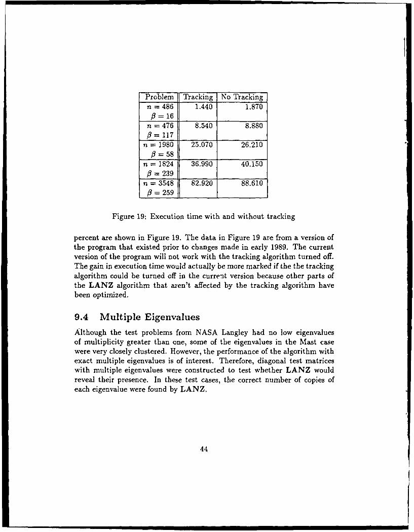
Figure 19: Execution time with and without tracking

percent are shown in Figure 19. The data in Figure 19 are from a version ofthe program that existed prior to changes made in early 1989. The currentversion of the program will not work with the tracking algorithm turned off.The gain in execution time would actually be more marked if the the trackingalgorithm could be turned off in the current version because other parts ofthe LANZ algorithm that aren't affected by the tracking algorithm havebeen optimized.

9.4 Multiple Eigenvalues

Although the test problems from NASA Langley had no low eigenvaluesof multiplicity greater than one, some of the eigenvalues in the Mast casewere very closely clustered. However, the performance of the algorithm withexact multiple eigenvalues is of interest. Therefore, diagonal test matriceswith multiple eigenvalues were constructed to test whether LANZ wouldreveal their presence. In these test cases, the correct number of copies ofeach eigenvalue were found by LANZ.

44

10 Concluding Remarks

10.1 Conclusions

For the large, generalized eigenvalue problem arising from two structuralengineering applications, the vibration and buckling problems, the LANZalgorithm was shown to be superior to the subspace iteration method. Re-sultP from sev'ral str,'ctura! engineering prcb!:ms were given to suppc. L tLL,claim. LANZ is based on the Lanczos algorithm and makes use of spectraltransformations, dynamic movement of a shift, and a modified version ofselective reorthogonalization to quickly converge to desired eigenpairs. Thedynamic shift-moving algorithm used by LANZ was described. The shifting-moving algorithm is based on a cost analysis of the Lanczos algorithm withspectral transformations and selective reorthogonalizations. A parallel algo-rithm for efficiently solving the tridiagonal matrices that arise when usingLanczos's method was also given.

10.2 Future Work

LANZ has been shown to perform well on vector machines, an importantclass of scientific computing machines. These classes show the most promisefor solving very large problems. The next step is to shown that LANZ willperform well on parallel and vector/parallel computers. An examination ofthe LANZ algorithm based on the analysis in Section 6 is the logical firststep in determining a strategy for parallelizing LANZ. A possible next stepis to use the Force programming language to parallelize the code [Jor87].This language allows parallel loops to be easily expressed and can be usedon several different shared-memory computers. The Force has been shownto be a good language for parallel linear algebra applications [JPV89]. The

outlined approach would most likely provide a good barometer with whichto assess the performance of LANZ on parallel machines.

Acknowledgements The authors would like to thank Dr. Axel Ruhefor several comments that led to the improvement of Section 5. The authorswould also like to thank Dr. Robert M. Jones whose comments were helpfulthroughout the paper and especially improved Section 2.

45

References

[Bat82] K. Bathe. Finite Element Procedures in Engineering Analysis.Prentice-Hall, Englewood Clifs, NJ, 1982.

[BG76] Victor Barwell and Alan George. "A Comparison of Algo-rithms for Solving Symmetric Indefinite Systems of Linear Equa-tions". ACM Transactions on Mathematical Software, 2(3):242-Z101, September 1976.

[BH87] Charles P. Blankenship and Robert J. Hayduk. "Potential Su-percomputer Needs for Structural Analysis". Presentation atthe Second International Conference on Supercomputing, May

3-8 1987. Santa Clara, CA.

[BK77] James R. Bunch and Linda Kaufman. "Some Stable Methodsfor Calculating Inertia and Solving Symmetric Linear Systems".Mathematics of Computation, 31(137):163-179, January 1977.

[BKP76] J. Bunch, L. Kaufman, and B. Parlett. "Decomposition of aSymmetric Matrix". Numerische Mathematik, 27:95-109, 1976.

(Cor87] Convex Corporation. CONVEX FORTRAN User's Guide, 1987.Dallas, TX.

[CW85] Jane K. Cullum and Ralph A. Willoughby. Lanczos Algorithmsfor Large Symmetric Eigenvalue Computations: Vol I Theory.Birkhauser, Boston, MA, 1985.

[ER80] Thomas Ericsson and Axel Ruhe. "The Spectral Transforma-tion Lanczos Method for the Numerical Solution of Large SparseGeneralized Symmetric Eigenvalue Problems". Mathematics ofComputation, 35(152):1251-1268, October 1980.

[GL83] Gene H. Golub and Charles F. Van Loan. Matrix Computations.The Johns Hopkins University Press, Baltimore, MD, 1983.

[GU77] G. H. Golub and R. Underwood. "The Block Lanczos Methodfor Computing Eigenvalues". In J. Rice, editor, MathematicalSoftware III, pages 361-377. Academic Press, New York, 1977.

46

[HWHB86] L. G. Horta, J. L. Walsh, G. C. Horner, and J. P. Bailey. "Anal-ysis and Simulation of the MAST (COFS-1 Flight Hardware)".NASA CP 2447, Part I, pages 515-532, Nov. 18-21, 1986.

[Jon89] Robert M. Jones. Personal communciatioi, 1989. Virginia Poly-technic Institute, Blacksburg, VA.

[Jor87] Harry Jordan. "The Force". Computer systems design group,University of Colorado, 1987.

[JPar] Mark T. Jones and Merrell L. Patrick. "Bunch-Kaufman Factor-ization for Real Symmetric Indefinite Banded Matrices". Tech-nical report, Institute for Computer Applications in Science andEngineering (ICASE), NASA Langley Research Center, Hamp-ton, VA, 1989 to appear.

[JPV89] Mark T. Jones, Merrell L. Patrick, and Robert G. Voigt. "Lan-guage Comparison for Scientific Computing on MIMD Architec-tures". Report no. 89-6, Institute for Computer Applicationsin Science and Engineering (ICASE), NASA Langley Research

Center, Hampton, VA, 1989.

[Kan66] Shmuel Kaniel. "Estimates for Some Computational Techniquesin Linear Algebra". Mathematics of Computation, 20:369-378,1966.

[Kni89] Norman Knight. Personal communciation, 1989. ComputationalStructural Mechanics, NASA Langley Reseach Center, Hamp-ton, VA.

[Lan50] Cornelius Lanczos. "An Iteration Method for the Solution of theEigenvalue Problem of Linear Differential and Integral Opera-tors". Journal of Research of the National Bureau of Standards,45(4):255-282, October 1950.

[Ma88] Shing Chong Ma. "A Parallel Algorithm Based on the SturmSequence Solution Method for the Generalized Eigenproblem,Ax = ABx". Master's thesis, Department of Computer Science,Duke University, 1988.

47

[Mah87] Umesh Mahajan. "Parallel Subspace Iteration for Solving theGeneralized Eigenvalue Problem". Master's thesis, Departmentof Computer Science, Duke University, 1987.

[NOC85] Bahram Nour-Omid and Ray W. Clough. "Block LanczosMethod for Dynamic Analysis of Structures". Earthquake Engi-neering and Structural Dynamics, 13:271-275, 1985.

[NOPEJ87] Bahran Nour-Omid, Beresford N. Parlett, Thomas Ericsson,-i d P :_1 S. J..... "F'w to _Trplement the Spectral Transfor-mation". Mathematics of Computation, 48(178):663-673, April1987.

(NOPT83j Bahram Nour-Omid, Beresford N. Parlett, and Robert L. Tay-lor. "Lancz,7s Versus Subspace Iteration For Solution of Eigen-value Problems". international Journal for Numerical Methodsin Engineering, 19:859-871, 1983.

[Pai7l] C. C. Paige. The Computations of Eigenvalues and Eigenvec-tors of Very Large Sparse Matrices. PhD thesis, Instiufe ofComputer Science, University of London, 1971.

[Par80] B. IN. Parlett. The Symmetric Eigenvalue Problem. Prentice-Hall, Englewood Cliffs, NJ, 1980.

(PNO85] Beresford N. Parlett and Bahram Nour-Omid. "The Use of aRefined Error Bound When Updating Eigenvalues of Tridiago-nals". Linear Algebra and its Applications, 68:179-219, 1985.

[PS79] B. N. Parlett and D. S. Scott. "Lanczos Algorithm With Selec-tive Orthogonalization". Mathematics of Computation, 33:217-238, 1979.

[Ruh74] Axel Ruhe. "SOR-Methods for the Eigenvalue Problemwith Large Sparse Matrices". Mathematics of Computation,28(127):695-710, July 1974.

[Ruh89] Axel Ruhe. Personal communciation, 1989. Department of Nu-merical Analysis, University of Umea, Umea, Sweden.

48

[Saa80] Y. Saad. "On The Rates of Convergence of the Lanczos and the Block-LanczosMethods." SIAM Journal of Numerical Analysis, 17(5):687-706, October 1980.

[Sch74) H. R. Schwarz. "The Method of Coordinate Overrelaxation for (A - AB)x =

0". Numerische Mathematik, 23:135-151, 1974.

[Sch89] H. R. Schwarz. "Rayleigh Quotient Minimization with Preconditioning".Journal of Computational Physics, 81:53-69, 1989.

[Sim84] Horst D. Simon. "The Lanczos Algorithm With Partial Reorthogonalization".Mathematics of Computation, 42:(165):115-142, January 1984.

[Ste89a Caroline B. Stewart. "The Computational Structural Mechanics Testbed Pro-cedure Manual", 1989. Computational Structural Mechanics, NASA LangleyResearch Center, NASA TM-100646, Hampton, VA.

[Ste89b] Caroline B. Stewart. "The Computational Structural Mechanics TestbedUser's Manual", 1989. Computational Structural Mechanics, NASA LangleyResearch Center, NASA TM-100644, Hampton, VA.

[SW82] Ahmed H. Sameh and John A. Wisniewski. "A Trace Minimization Algo-rithm for the Generalized Eigenvalue Problem". SIAM Journal of NumericalAnalysis, 19(6):1243-1259, December 1982.

[Szy831 Daniel B. Szyld. A Two-level Iterative Method for Large Sparse GeneralizedEigenvalue Calculations. Ph.D thesis, Department of Mathematics, New YorkUniversity, 1983.

[Wi165] J. H. Wilkinson. The Algebraic Eigenvalue Problem Oxford University, Ox-ford, 1965.

49

A Sequential and Vector Cost Analysis

A step-by-step cost analysis for the Lanczos algorithm when using trans-formation B (shown in Figure 2) is given below for sequential and vectormachines.

Definitions:AK: The semi-bandwidth of the K matrix.IM: The semi-bandwidth of the Al matrix.n: The number of eauations in the system.daxpy: A double precision vector operation that computes ax-ry,

where a is a scalar and x and y are vectors.

Initialization1.) Choose an initial guess, guess

Small cost (O(cn)), but might be larger depending on themethod used for choosing the guess.

2.) r0 = (K - aM)-'Mgues (Purifying ro)A.) Formation of the matrix (K - aM)

The matrix is formed from K and M and made availableto the factorization routine.Sequential. pmn subtractions and multiplicationsVector: 1 pzMn-length daxpy operation

B.) Factorization of (K - o'M)Using Bunch-Kaufman (or LDLT decomposition) as de-scribed in Section 8Sequential: n divisions

O(npK) multiplicationsO(nP2/2) multiplications and additions

Vector: n scalar divisionsn 1K-length vector by scalar multiplicationsnP1K daxpy operations of avc;-age length IK

C.) Forward Solve using factored matrix from BSequential: O(n1K) multiplications and divisionsVector: n YK-length daxpy operations

D.) Diagonal Solve using factored matrix from BSequential: 3n multiplications

50

2n additionsVector: 3 n-length daxpy operations

E.) Back Solve using factored matrix from BSequential: O(nuK) multiplications and divisionsVector. n p--length inner products

3.) Pi = AfroAn n x n banded matrix-vector multiplicationSequential: O((2PK + 1)n) multiplications

O(21UKn) additionsVector: n pK + 1-length inner products

n /K-length daxpy operations4.) I8 = (ropl)1/2

An n-length inner product and a square rootSequential: n multiplications

n - 1 additions1 square roct

Vector. 1 n-length inner product1 square root

Program Loop5.) For j = 1, maximum number of iterations6.) Reorthogonalization phase

Orthogonalize rpi- and q,-, against "good" Ritz vectorsif necessary (see section on orthogonalization for details).Steps A and B are done only once and only if reorthog-onalization is needed. Steps C and E are done for eachRitz vector that is orthogonalized against rj-1. Steps Dand F are done for each Ritz vector that is orthogonalizedagainst qj-,.A.) tj = Mrj-l

Same cost as 3B.) t2 = Mqj- 1

Same cost as 3C.) Yi = yft1

Multiplication of an n-length vector by a scalarSequential: n multiplications

51

Vector: 1 n-length vector by scalar multiplicationD.) ¢ = yft 2

Same cost as CE.) rj-1 = rj- 1 - iyi

Orthogonalize rj against y,Sequential: n multiplications

n additionsVector. 1 n-length daxpy operation

F.) qj-1 = q-- ikiySame cost as 6EOrthogonalize rj against y,

7.) qj =ri_,/ l

Division of an n-length vector by a scalarSequential. n multiplications

1 divisionVector. 1 n-length vector by scalar multiplication

1 division8.) pj = pj/ j

Same cost as 79.) (K - uM)rj = pi

Same cost as parts C, D, and E of 310.) rj = rj - qj-llj

Orthogonalize rj against qj-1Same cost as 6E

11.) = T

Same cost as 4 except no square root is needed12.) rj = rj - qjaj

Same cost as 1013.) pj+l = Mri

Same cost as 314.) g,+, = (rp,+,)1/2

15.) Compute the eigenvalue of Tj and the corresponding error bounds

A.) Calculate j eigenvalues via Newton's methodSequential and Vector. Variable, but very small (0(j32 ))

B.) Calculate j error bounds, 3jiSequential: j multiplications

52

16.) Compute any converged Ritz VectorsCost per Ritz vector of computing y,A.) Compute correction factor, wi = 1/0j(Tjsj)

Sequential: 3j multiplications2j additionsj multiplications1 division

Vector. 3 j-length daxpy operations1 j-length vector by scalar multiplication1 division

B.) Compute y, = Qj+jwjSeque-ntial: nj multiplications

n(j - 1) additionsVector. n j-length inner products

17.) Halt if enough eigenvalues have been found18.) End of Loop

53

Axially- Comnpressed Cylinder

Lp

R

-~ 6V Model for SMOOTH Mode

(uniform) 15' Model-for OIAMONO/AXI.SYM. Modes

(R/h 300) (L/R =3)

]Figure 20: Axi ally- compressed circular cylindrical shell

54

Figure 21: Lowest two buckling modes of an axially-compressed cylinder

55

Figure 22: Composite blade-stiffened panel with a discontinous stiffener

56

II

w77,3"A

F ,'lre 23: Deployable space mast

57

NReport Documentation Page1. Report No. 2. Government Accession No. 3. Recipient's Catalog No.

NASA CR- 181914ICASE Report No. 89-69

4, Title and Subtitle 5. Report Date

THE USE OF LANCZOS'S METHOD TO SOLVE THE LARGE 'eterher 1989GENERALIZED SYMMETRIC DEFINITE EIGENVALUE PROBLEM 6. Performing Organization Code

7. Author(s) 8. Performing Organization Report No.

Mark T. Jones 89-69Merrell L. Patrick 10. Work Unit No.

9. Performing Organization Name and Address 505-90-21-01Institute for Computer Applications in Science 11. Contract or Grant No.

and EngineeringMail Stop 132C, NASA Langley Research Center NASI-18605Hampton, VA 23665-5225 13. Type of Report and Period Covered

12. Sponsoring Agency Name and Address

National Aeronautics and Space Administration Contractor ReportLangley Research Center 14. Sponsoring Agency Code

Hampton, VA 23665-5225

15. Supplementary Notes

Langley Technical Monitor:Richard W. Barnwell

Final Report16. Abstract

The generalized eigenvalue problem, KX = XMX, is of significant practicalimportance, especially in structural engineering where it arises as the vibrationand buckling problems. A new algorithm, LANZ, based on Lanczos's method isdeveloped. LANZ uses a technique called dynamic shifting to improve the efficiencyand reliability of the Lanczos algorithm. A new algorithm for solving thetridiagonal matrices that arise when using Lanczos's method is described. Aodification of Parlett and Scott's selective orthogonalization algorithm isproposed. Results from an implementation of LANZ on a Convex C-220 show it to besuperior to a subspace iteration code.

17. Key Words (Suggested by Authorls)) 18. Distribution Statement

generalized eigenvalue problem, 61 - Computer Programming and Software

Lanczo's method, buckling and vibration 64 - Numerical Analysis

problems 39 - Structural Mechanics

Unclassified - Unlimited19. Security Classif. (of this report) 20. Security Classif. (of this page) 21. No. of pages 22. Price

Unclassified Unclassified 59 A04

NASA FORM 1626 OCT 86

NASA-Langley, 1g8g