Embed Size (px)
Citation preview

/
Report No. UMTA-VA-06-0053-79-1
36 • 1
R€CE\V€.D
~\i ,: 1 1979
L\BRARY
The Status of Advanced Propulsion Systems
fo r Urban Rail Vehicles
MAY 1979
Document is Available to the U.S. Public Through The National Te chnical Information Service, Springfield, Virginia 22161
Prepared for
U.S. D-2partm 2nt of Transportation Urban Mass Transporta tion Administration Office of Technology D13velopment & Deployment Office of Rail and Con3truction Technology
Washington, D. C. 20530
RECEIVED
AUG 1 0 1979 LIBRARY

' ✓
NOTICE
This document is disseminated under the sponsorship of the
Department of Transportation in the interest of information
exchange. The United States Government assumes no
liability for its contents or use thereof.
NOTICE
The United States Government does not endorse products or
manufacturers. Trade or manufacturers' names appear herein
solely because they are considered essential to the object of
this report.

1. Report No. 2. Government Accession No.
UMTA-VA-06-0053-79-1
4. Title ond Subtitle
THE STATUS OF ADVANCED PROPULSION SYSTEMS FOR URBAN RAIL VEHICLES
Technical ~eport Documentation Page
3. Recipient's Cotolog No.
S. Report Dote
May 1979 6. Performing Orgonizotion Code
MTR-79W0022 t--;;-;--:-;--,-_--------------------------1 8. Performing Orgonizotion Report No.
7. Authorls) V. D. Nene
9. Performing Orgoni zation Nome ond Address
The MITRE Corporation 1820 Dolley Madison Boulevard McLean, Virginia 22101
12. Sponsoring Agency Nome and Address
U.S. Department of Transportation Urban Mass Transportation Administration 400 Seventh Street, S.W. Washington, D. C. 20590
15. Supplementary Notes
16. Abstract
10.
11.
13.
14.
Work Unit No. (TRAIS)
VA-06-0053 Controct or Grant No.
DOT-UT-9002 Type of Report and Period Covered
Final Technical Report Oct. 1978 - May 1978
Sponsoring Agency Code
UTD-30
Rheostatic control of de traction motors has been in use for several decades. With the advent of power electronics, however, more efficient alternate propulsion systems have been developed. These include chopper controls, ac drive with induction motors, systems using onboard energy storage and ac drive with tubular axle motors. Of these concepts, chopper controllers have been in regular revenue service for several years while others are still under prototype testing.
This report describes in detail the status of all these propulsion systems. The performance characteristics, the significant advantages and disadvantages and the deployment of the hardware in revenue service for all these systems is discussed. The report concludes with a general description of alternate traction motors and power converters.
This report is a technology review of advanced traction systems. It is based on information and data gathered from propulsion equipment suppliers in Europe, Japan, and the United States.
17. Key Words
Propulsion Systems Traction Systems Power Electronics Motors Urban Rail Vehicles
19. Security Classif. (of this report)
Unclassified
Form DOT F 1700.7 C8-72l
18. Distribution Statement
AC Drives Choppers
Available to the Public through the National Technical Information Service, Springfield, Virginia 22161.
20. Security Classif. (of this page)
Unclassified
Reproduction of completed page outhori zed
21, No. of Pages 22. Price
213

MITRE Technical Report MTR-79W00022
The Status of Advanced Propulsion Systems
for Urban Rail Vehicles Interim Report .
Vilas D. N ene
February 1979
Contract Sponsor: U MTA Contract No.: DOT-UT 90002
Project No.: 12490 Dept. W-23
The MITRE Corporation Metrek Division
1820 Dolley Madison Boulevard McLean, Virginia 22102

01961
TF -4~55 .N36

ABSTRACT
Rheostatic control of de traction motors has been in use for several decades. With the advent of power electronics, however, more efficient alternate propulsion systems have been developed. These include chopper controls, ac drive with induction motors, systems using onboard energy storage and ac drive with tubular axle motors. Of these concepts, chopper controllers have been in regular revenue service for several years while others are still under prototype testing. This interim report describes in detail the status of all these propulsion systems. The performance characteristics, the significant advantages and disadvantages and the deployment of the hardware in revenue service for all these systems is discussed. The report concludes with a general description of alternate traction motors and power converters. The final version of this report will include - similar assessment of the status of linear motor propulsion systems, monomotor and radial trucks and a summary of other propulsion activities in the area of high speed ground transportation.
iii

ACKNOWLEDGEMENT
The author wishes to express his sincere thanks for the total access to the technical information extended to him by the following companies and organizations. He would also like to thank many of these organizations for the welcome extended to him during his visits and the long hours spent by their technical people during these visits.
These are: In the U.S. - GE, Westinghouse, and Garrett Corporation, NYCTA and BART. In Europe - ASEA (Sweden), Stromberg (Finland), BBC, Siemens and AEG (Germany), Alsthom (France), The French National Railways (SNCF), and the Railway Technical Center of the British Rail (U.K.). In Japan - Mitsubishi, Hitachi and Fuji Corporation.
Such a status report is clearly impossible without such cooperation.
The author also would like to thank Mr. H. Lee Tucker of the U.S. DOT/UMTA for his continued interest and support for this work.
Thanks are also due to Mr. Carl Swanson of the MITRE Corporation for carefully going through the manuscript and making very valuable suggestions.
iv
TABLE OF CONTENTS
LIST OF ILLUSTRATIONS LIST OF TABLES GLOSSARY
1.0 INTRODUCTION
2.0 PROPULSION EQUIPMENT WITH A CAM CONTROLLER
2.1 Starting and Motoring Operation 2.2 Braking Operation 2.3 Types of Cam Controllers 2.4 Energy Consumption
3.0 CHOPPER CONTROLLED PROPULSION EQUIPMENT
3.1 Operation of a Chopper Controller 3.2 Deployment of Chopper Controllers 3.3 Field Control of Traction Motors 3.4 Energy Savings by Regeneration 3.5 Advanced Cooling Methods 3.6 Use of a Microprocessor
4.0 AC DRIVES USING INDUCTION MOTORS
4.1 AC Drives for Locomotives 4.2 Urban Vehicles 4.3 Effect of Unequal Wheel Diameters
5.0 AN AC DRIVE WITH A SYNCHRONOUS MOTOR
5.1 A Self-Synchronous Propulsion System 5.2 Propulsion System Specifications 5.3 System Components 5.4 Test Results 5.5 A Locomotive Application
6.0 PROPULSION SYSTEM WITH ONBOARD ENERGY STORAGE
6.1 R-32 Energy Storage Car for NYCTA 6.2 ACT-1 Propulsion System 6.3 Improved Propulsion System for R-36 Cars of NYCTA 6.4 Noise and Vibrations 6.5 Additional Maintenance 6.6 Gyroscopic Effects
V
Page vii
xiii xiv
1
2
2 4 5
12
17
18 21 32 35 40 45
47
48 53 66
70
70 72 73 77 83
84
86 92 98 98 98
101

TABLE OF CONTENTS (concluded)
7.0 TUBULAR AXLE INDUCTION MOTOR
7.1 Motor Design 7.2 Inverter Design
8.0 CONCLUSIONS
LIST OF REFERENCES
APPENDIX I - DIFFERENT TYPES OF TRACTION MOTORS
APPENDIX II - POWER CONVERSION DEVICES
vi
102
102 103
109
113
119
171
FIGURE NUMBER
1
2
3
4
5
6
7
8
9
10
11
12
13
14
15
16
17
18
19
20
21
22
LIST OF ILLUSTRATIONS
Starting and Motoring Circuit
Braking Circuit
Load Sharing Between Two DC Generators
Typical Braking Characteristics
A Camshaft System
A Cam Controller
A Contactor
Typical Resistor Assembly
Energy Flow for Rheostatic Control
WMATA Car
Voltage Control by a Chopper
A Chopper Controller
BART Car
Subway Car of Type C9
A Thyristor Module
Complete Chopper Equipment
Articulated Tramcar
Trolleybus with Chopper Control
Wuppertal Suspension Railway
MF77 Cars of Paris Metro
Three-Coach Unit of Lyons Metro
Monomotor Truck - Lyons Metro
vii
PAGE
3
6
7
8
8
9
10
13
14
15
19
20
23
24
24
26
26
27
30
30
31
31

FIGURE NUMBER
23
24
25
26
27
28
29
30
31
32
33
34
35
36
37
38
39
40
41
42
43
44
LIST OF ILLUSTRATIONS (continued)
Automatic Variable Field Control
Field Control by a Modified Shunt
Equivalent Circuits
Field Current Waveform
Field Weakening Ratio
Energy Flow for Regenerative Chopper
Freon Cooling Systems
Heat Transfer Characteristics
DE 2500 Locomotives with AC Drive
All Electric Locomotive with AC Drive
Dual Frequency Industrial Locomotive
Other Locomotives with AC Drive
Power Circuit of VL 80K
WABCO Propulsion System
Three Modes of Motor Operation
A Coach-Pair of Series MlOO
The Main Circuit of MlOO
Berlin Subway Vehicle with AC Drive
The Main Circuit Diagram
Twin Motor Unit of Squirrel Cage Traction Motors
AC Drive by Siemens
Pulsed Mode of Inverter Operation
viii
PAGE
33
36
37
38
38
41
43
44
49
51
51
52
54
55
56
59
59
61
61
64
64
68
FIGURE NUMBER
45
46
47
48
49
50
51
52
53
54
55
56
57
58
59
60
61
62
63
64
65
66
LIST OF ILLUSTRATIONS (continued)
Effect of Unequal Wheel Diameters
System Block Diagram - Motoring Mode
Line Filter
Dual Inductor Assembly
Inverter Circuit
Capacitor Module Circuit Diagram
Cycloconverter Power Circuit
AC Traction Motor
Motoring/Braking Test Results
Torque-Speed Characteristics for Constant Inverter Frequencies
Comparison of Braking Performance
Use of Onboard Energy Storage
R-32 Energy Storage Unit
Propulsion System Schematic
Power Flow During a Typical Run
Energy Savings by Onboard Flywheel System
Typical Energy Flow of a Flywheel Car
ACT-1 Energy Storage Unit
ACT-1 Vehicle
ACT-1 Propulsion System Schematic
R-36 Propulsion System Schematic
ESU for R-36
ix
PAGE
68
71
74
74
75
76
78
78
79
80
81
85
87
88
91
93
94
96
97
99
99
100

FIGURE NUMBER
67
68
69
70
71
72
73
74
75
76
77
78
79
80
81
82
83
84
85
86
87
88
LIST OF ILLUSTRATIONS (continued)
Speed Torque Characteristics
Partially Wound TAIM Primary and the Axle
Completed TAIM Primary
Squirrel Cage Secondary in the Hollow Axle
Completely Assembled TAIM
TAIM Mounted on a Vehicle
New TAIM Design
British Rail Research Vehicle
Essential Components of a DC Motor
DC Motor Schematic
Airgap Flux Distribution in a DC Machine
Current Reversal During Commutation
DC Motor with Interpoles and Compensating Windings
DC Motor Field Structure and Windings
Armature and Commutator of a DC Motor
The Brushgear
Methods of Field Excitation
Starting of a DC Motor
Speed Control of a DC Motor
Essential Components of an Induction Motor
A Squirrel Cage Rotor
Induction Motor Windings
X
PAGE
104
104
105
105
106
106
108
108
120
121
121
122
124
125
126
127
128
130
131
135
136
139
FIGURE NUMBER
89
90
91
92
93
94
95
96
97
98
99
100
101
102
103
104
105
106
107
108
109
110
LIST OF ILLUSTRATIONS (continued)
Equivalent Circuit
Torque and Current as a Function of Slip
Power Factor and Efficiency of Induction Motor
Speed Control for Traction Applications
Synchronous Motor Schematic
Synchronous Motor Phasor Diagrams
Use of Rotating Transformer/Rectifier
Synchronous Reluctance Motor
Vernier Motor
Doubly Slotted Structure of Vernier Motor
Homopolar Inductor Motor
Two Rotor Cores
Airgap Flux Density Distributions
Rice Motor
Lundell Motor
Operating Principle of a Chopper
Chopper Circuit and its Response
Different Modes of Chopper Operations
Chopper Commutation
Filter Response
Multi-Phase Chopper
Three Phase Bridge Rectifier
xi
PAGE
139
141
143
145
148
150
154
157
157
158
162
163
164
166
168
173
175
177
177
178
179
183
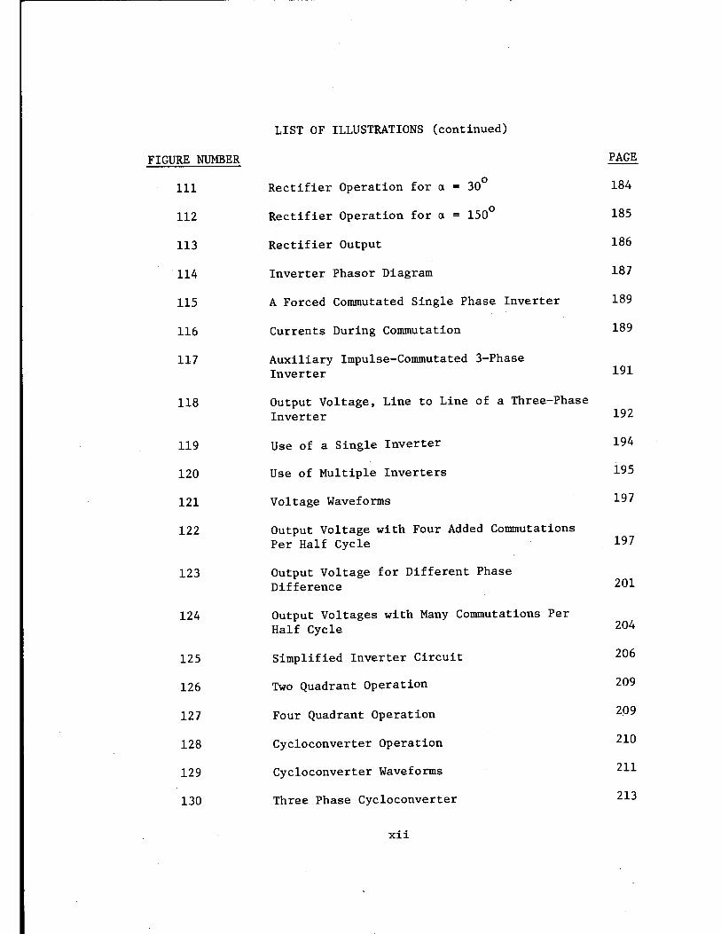
FIGURE NUMBER
111
112
113
114
115
116
117
118
119
120
121
122
123
124
125
126
127
128
129
130
LIST OF ILLUSTRATIONS (continued)
Rectifier Operation for a. = 30°
Rectifier Operation for a. = 150°
Rectifier Output
Inverter Phasor Diagram
A Forced Commutated Single Phase Inverter
Currents During Commutation
Auxiliary Impulse-Commutated 3-Phase Inverter
Output Voltage, Line to Line of a Three-Phase Inverter
Use of a Single Inverter
Use of Multiple Inverters
Voltage Waveforms
Output Voltage with Four Added Commutations Per Half Cycle
Output Voltage for Different Phase Difference
Output Voltages with Many Commutations Per Half Cycle
Simplified Inverter Circuit
Two Quadrant Operation
Four Quadrant Operation
Cycloconverter Operation
Cycloconverter Waveforms
Three Phase Cycloconverter
xii
PAGE
184
185
186
187
189
189
191
192
194
195
197
197
201
204
206
209
209
210
211
213

FIGURE NUMBER
131
TABLE NUMBER
I
II
III
IV
V
LIST OF ILLUSTRATIONS (concluded)
Full Wave Three Phase Circuit
LIST OF TABLES
Synchronous Machines
Synchronous Motors
Fundamental Amplitude Control by Varying a 1 and a 2
Elimination of the Fifth and Seventh Harmonics
Multiple Inverter Control with Elimination of the Third and Fifth Harmonics
xiii
PAGE
214
PAGE
152
169
199
200
203
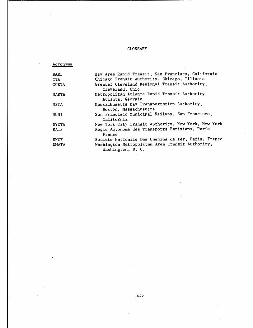
Acronyms
BART CTA GCRTA
MARTA
MBTA
MUNI
NYCTA RATP
SNCF WMATA
GLOSSARY
Bay Area Rapid Transit, San Francisco, California Chicago Transit Authority, Chicago, Illinois Greater Cleveland Regional Transit Authority,
Cleveland, Ohio Metropolitan Atlanta Rapid Transit Authority,
Atlanta, Georgia Massachusetts Bay Transportation Authority,
Boston, Massachusetts San Francisco Municipal Railway, San Francisco,
California New York City Transit Authority, New York, New York Regie Autonome des Transports Parisians, Paris
France Societe Nationale Des Chemins de Fer, Paris, France Washington Metropolitan Area Transit Authority,
Washington, D. C.
xiv
1.0 INTRODUCTION
This report summarizes the status of advanced propulsion concepts
required for the ASDP Propulsion Assessment Study (Task 2, State-of
the-Art Assessment). The assessment covers the technical performance,
reliability, maintainability, safety features and deployment status
of traction systems using chopper controlled de motors, three phase
induction motors, self-synchronous motors, flywheel energy storage
systems, and tubular axle motors.
DC series motors have been used as traction motors almost exclu
sively since the early days of electric propulsion of rail vehicles.
This is because the torque-speed characteristic of the motor is extre
mely well-suited for traction applications and the speed can be
controlled very easily by using series/parallel connections of several
motors or by using external resistances. Inherent inefficiency of the
rheostatic control and excessive maintenance costs for the commutator
of the traction motor are the two major problems associated with this
conventional traction technology. Recent advances in thyristor tech
nology have made it possible to develop new efficient traction systems
requiring less maintenance, with a reduction of overall life-cycle costs.
Chopper control of de motors and pulse-width modulated inverter .control
of induction motors are two examples. Other concepts include hybrid
systems using flywheel energy storage, tubular axle motors, and ac
self-synchronous motors. Thus, the technical problems that are of the
greatest concern to rapid rail transit operators can be addressed by
this existing technology, resulting in ~mprovements that can be
deployed to transit properties in the near term.
This report is a technology review of these advanced traction sys
tems. It is based on information and data gathered from propulsion
equipment suppliers in Europe, Japan and the U.S.
1
2.0 PROPULSION EQUIPMENT WITH A CAM CONTROLLER
Speed control of de traction motors over a wide range essentially
involves "armature control" for speeds below the base speed and "field
control" for speeds above the base speed. The classical method is
rheostatic control, accomplished by using external resistances in
series with armature and in parallel with the field winding. By con
trolling these resistances, one can control both the armature current
and the field current of the motor. In a transit car, armature control
can also be achieved by series/parallel connections of the four traction
motors on the car. With a cam controller, this rheostatic control is
obtained by means of contactors actuated by a shaft. Although pneu
matically operated cams were introduced as early as almost 60 years
ago, cam control with an electric motor driven camshaft has been in
use since early 1950's. (l-4)
2.1 Starting and Motoring Operation
The simplified circuit diagram of Figure 1 shows how the traction
motors I-IV are controlled during starting and motoring operation.
Contactors 6-19 are used to insert the appropriate resistances in
the circuit. If the switches 1, 2, 3 and 6, 9 are closed, the four
traction motors are in series and the starting resistance in the
circuit is maximum. If, however, 1, 3, 4, 5 and 6, 9 are closed,
the motors are in a series-parallel connection, where the motors
I and II are in series with each other and they are in turn parallel
to the series connection of the motors III and IV. After the starting
resistors are shorted, this series-parallel connection is the final
operating connection for motoring region. The field weakening is
then achieved at high speeds by shunting the field as required by
closing the appropriate contactor from contactors 12-19. It should
be seen here that even a simple control as described above requires
the use of several contactors.
2

w
V ► 1
6
FIELD SHUNT STARTING RESISTORS
5
STARTING RESISTORS FIELD SHUNT 1\/V'Nv,
l6L3-~ I 9 po(n( L--L-.JVV'.~
FHI
FIGURE 1 STARTING AND MOTORING CIRCUIT
2 / /4
\ f • \ I 3~1•

2.2 Braking Operation
In general, two modes of braking operation are possible when the
kinetic energy of the car is converted to electrical energy by using
the traction motors as generators. In the regenerative braking mode
electrical energy is in part returned to the source voltage; in a
dynamic braking mode the electrical energy is dissipated in braking
resistors. The following considerations, however, tend to limit the
regeneration capability of rheostatic control:
a. Voltage rise on the third rail: Whenever energy is fed back to the system, the traction motor has to generate voltages higher than the voltage of the third rail. The voltage difference required depends on the impedance between traction motor as a source and the wayside system as a sink of the energy being transferred. Because of the characteristics of the existing wayside and onboard equipment, the maximum voltage to which the system could be subjected during regeneration is severely limited.
b. Stepped Control: The cam controller switches a finite number of resistances in and out of the armature and the field circuit as required. The control, therefore, is stepped and not smooth. Hence, the motor voltage cannot be continuously matched with the braking requirements.
Considering all the factors involved, use of regenerative
braking with cam controllers cannot be economically justified for
retrofitting existing transit systems or on new systems. One can,
however, add static controllers to obtain regenerative braking of
the traction motors on a cam controlled car. In such a system all
the traction motors can be connected in series while their fields are
separately excited to control the braking action. Braking is smooth
because of the solid state control and it can be seen that it is no
longer "cam controlled" in the true sense of the words. Such a
system is, is fact, in use on commuter cars in Australia.
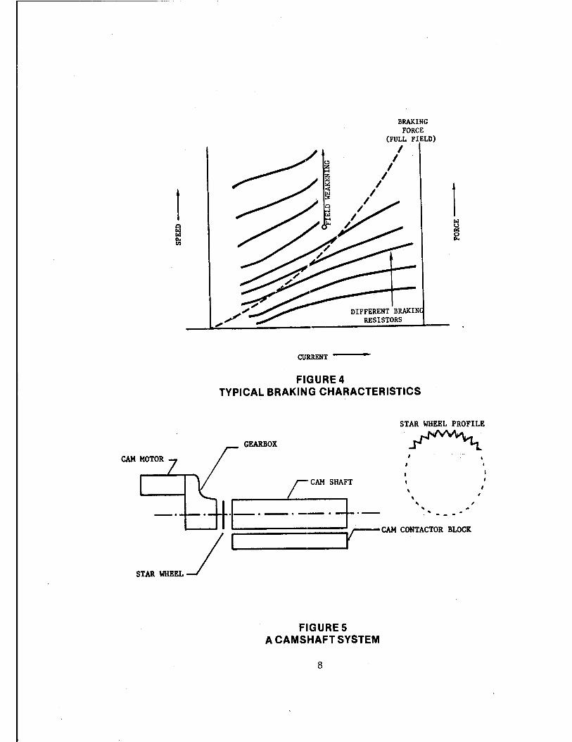
For dynamic braking, the traction motors operate as de genera
tors, converting the kinetic energy of the vehicle to electrical
4

energy that is dissipated in braking resistors. The braking force
is controlled by controlling the braking resistor and by field shunt
ing. Figure 2 shows such an operation. Here motors I and II are
connected in series, and these in turn are connected in parallel to
motors III and IV in series. Whenever two sources are connected in
parallel to feed a load, the load sharing depends on the loading
characteristics - the regulation of these sources. For example,
Figure 3(a) shows two de generators feeding power into the load. The
V-I characteristics of these two generators are shown in Figure 3(b).
For any load voltage v1
, the load on each generator can be obtained
as shown in the figure. For de generators, equal load sharing can
be ensured by cross-connecting the field windings - the field winding
of 1 being excited by the armature current of 2 and vice versa.
Under these conditions, the V-I characteristic of each generator is
controlled by the load on the other as shown in Figure 3(b) and the
load current is shared equally between the two generators. This is
precisely why the field windings in Figure 2 are cross-connected for
dynamic braking. A set of typical braking force characteristics are
shown in Figure 4.
2.3 Types of Cam Controllers
Figure 5 shows a simplified camshaft system with a camshaft driven
by an electric motor through a gear box. The star wheel enables
accurate and quick positioning of camshaft in each step. Further
details of the cam controller are shown in Figure 6 and a contactor
is shown in Figure 7.
Smoothness of control, response time and retrogression capability
are some of the important characteristics of a cam controller. A cam
control is essentially a stepped control and hence, smoothness of
control is directly related to the number of steps or notches in the
control. A large number of notches results in a longer camshaft. The
5

FIELD SHUNT FII
FI
°'
FIII FIELD SHUNT
FIV
. FIGURE2 BRAKING CIRCUIT
BRAKING RESISTOR

IL
11 I 121
(a) Electrical Circuit
CHARACTERISTIC SHIFTS , "
FOR 11 > ~ ,,,,,'
V-I CHARACTERISTIC, OF GEN. 2 , ' , ,
, ,
I 1 LOAD r- ON 2 I I
(b) Regulation Characteristics
FIGURE 3
LOAD
LOAD SHARING BETWEEN TWO DC GENERATORS
7
T VL
1
V-I CHARACTERISTIC OF GEN. 1
I
CURRENT
FIGURE 4
DIFFERENT BRAKIN RESISTORS
1
TYPICAL BRAKING CHARACTERISTICS
STAR WHEEL PROFILE
---'--,....... r GEARBOX CAM MOTOR /
~ ' • r: CAM SHAFT • • ,
·I-·-·--·+·- --. -- ___ , 1
, ..... ________ _,rCAM CONTACTOR BLOCK
STAR WHEEL_/
FIGURES A CAMSHAFT SYSTEM
8

9

FRAME---------
MAIN HINGE PIN
BLOWOUT COIL
STATIONARY CONTACT
------ MOVING CONTACT
---- INTERLOCK MOVING CONTACT ASSEMBLY
INTERLOCK STATIONARY CONTACT ASSEMBLY.
FIGURE 7 ACONTACTOR
10
response ti~e of the controller is related to the speed with which
circuit changeovers can be made. This response time can be reduced
either by adding more contacts on the camshaft (this would increase
its length) or by having a second motor driven cam. One camshaft
can control only the resistors and the other shaft can control the
contacts for circuit changeovers. Alternately one camshaft can con
trol the motoring and the other can control the braking operation.
In such a case, while the control is in motoring, the brake controller
can be continuously "spotted," i.e., be ready with the required circuit
connections depending on the vehicle speed. Another important charac
teristics of a cam controller is the possibility of retrogression.
Earlier cam controllers achieved power modulation only by forward
progression of the control. Any power reduction was possible only
by opening the line switches or in some cases by momentarily inserting
resistance before opening the line. New designs of cam controllers,
however, make it possible to modulate power by either forward motion
(progression) or by backward motion (retrogression) of the controller.
With full retrogression, it is possible to get back to series motor
connection from parallel connection and also have full field or weak
field. With such a control it is nece,ssary to equip all the main
contractors with arc blow-out chutes.
The total propulsion system hardware includes several components
which are not shown in Figures 1 and 2. For example, typical cam
controlled propulsion equipment for transit vehicles will have
following major components:
a. Manual master controller.
b. Four drive assemblies on each car, each consisting of a traction motor, gear unit, ground brush holder, speed sensors and other support hardware.
c. Main controller on each car consisting of line switches, cam drive, contactors, relays, series-parallel controller, field shunt, power-brake controller, fuse box, limit relay, control logic, etc.
11

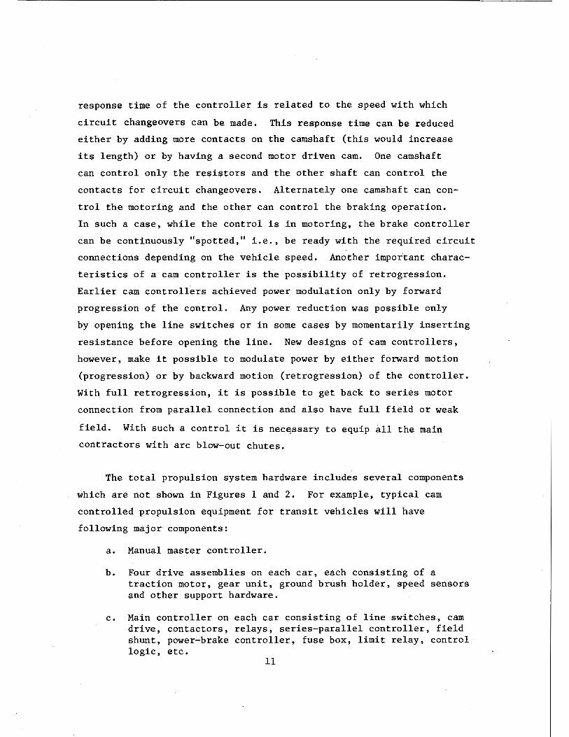
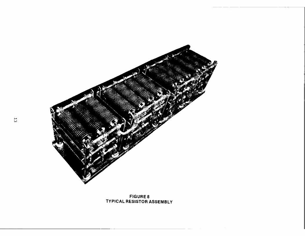
d. Set of accelerating and dynamic braking resistors consisting of many tube assemblies as shown in Figure 8. Each tube shown in the figure could be 12-18 inches long.
It also has several other components such as a cooling system, air
filters, a brake system and its mounting, etc.
2.4 (5,6) Energy Consumption
The typical rheostatic control of traction motors is very
inefficient. All the energy which is required to accelerate a
vehicle is lost. A certain amount is dissipated in starting resistors
and the rest is stored as kinetic energy in the vehicle. This kinetic
energy is then dissipated in braking resistors when the vehicle is
brought to a stop. Also, the traction motor, the onboard auxiliaries,
the substations and the third rail have electrical losses. The energy
required to maintain the cruise speed of the vehicle is quite small
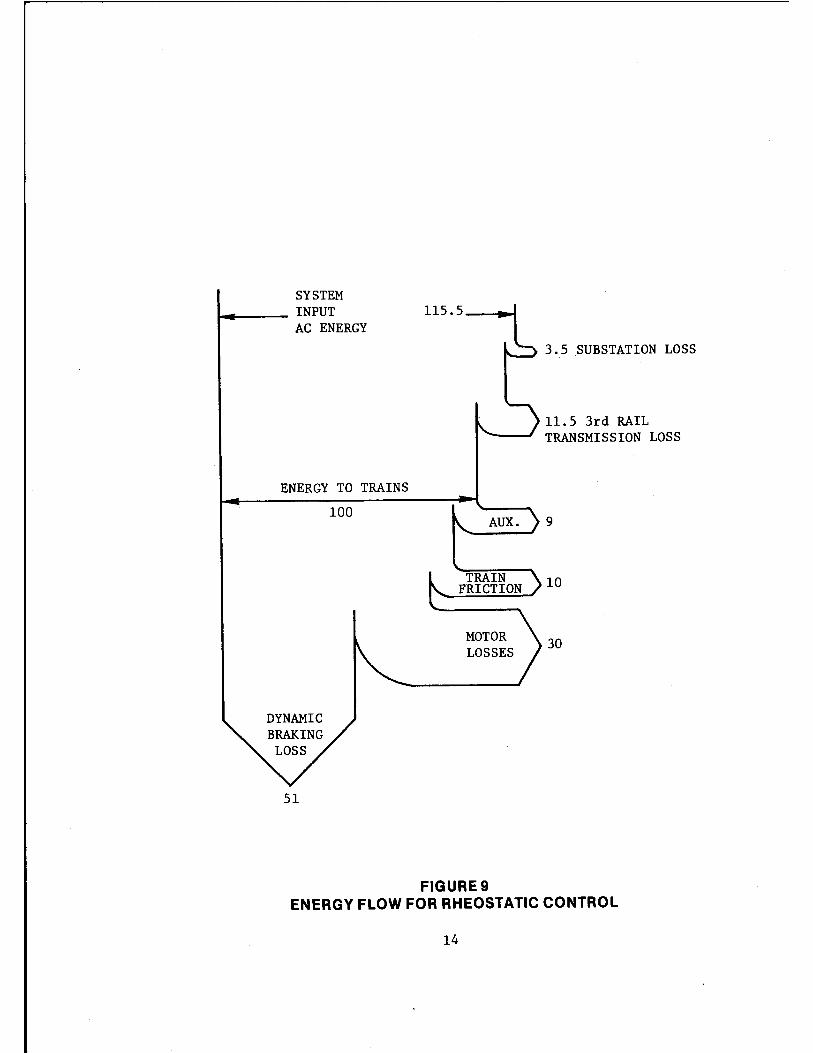
compared to the total energy consumption. The actual dissipation of
energy in the above components is highly dependent on the duty cycle
and hence, it is difficult to quote a typical distribution. Figure 9
shows the results of a specific computer simulation of transit opera
tions in the Northern Queens area of NYCTA(5). One can get a fairly
good idea of the relative share of different losses from this figure.
There are virtually thousands of transit and commuter cars
around the world using cam controller propulsion equipment. In fact
more than 1500 cars with such equipment were purchased by U.S. pro
perties alone since 1972. These include 754 R-46 cars by NYCTA, New
York (1972), 200 cars by WMATA, Washington D.C. (1973), 190 cars by
CTA, Chicago (1974) and 190 cars by MBTA, Boston (1976). Figure 10
shows the WMATA car.
In conclusion, it can be said that the cam control is a very
well proven technology and the control system is fairly simple. High
12
1--' w
FIGURES TYPICAL RESISTOR ASSEMBLY
SYSTEM ~--- INPUT
AC ENERGY
ENERGY TO TRAINS
100
DYNAMIC
51
AUX.
TRAIN FRICTION
MOTOR LOSSES
FIGURE 9
3.5 SUBSTATION LOSS
11.5 3rd RAIL TRANSMISSION LOSS
9
10
30
ENERGY FLOW FOR RHEOSTATIC CONTROL
14

r-' Vl
FIGURE 10 WMATACAR

energy consumption, maintenance and inspection (M&I) costs associated
with the contactors, the control circuits and the de traction motors,
however, are the major disadvantages of such equipment.
16

3.0 CHOPPER CONTROLLED PROPULSION EQUIPMENT
The basic function of any propulsion control is to regulate the
motoring and braking performance of the traction motors as required.
A rheostatic controller regulates the voltage applied to the motor
by using external resistances in series with the armature. A chopper
control is another means of controlling the armature voltage of a de
traction motor while eliminating the relatively large control steps
and resistor losses associated with rheostatic control. A chopper
has three basic capabilities beyond the resistor control. First is
the ability to regulate speed with a stepless control, thus elimi
nating the jerk associated with on-off control. The steady motor
torque improves the vehicle performance when operating under automatic
control and reduces slipping and sliding tendencies, permitting
better utilization of adhesion. Secondly, the chopper control being
a voltage control, the line current drawn is proportional to power
rather than to torque as with a rheostatic control, resulting in
load reduction during motoring. Finally is the ability to control
regeneration and return part of the kinetic energy of the vehicle to
the line during braking.
Since the early days of electric traction, it was realized that
a variable voltage de source can be used to efficiently control the
speed of the de traction motor. In fact, a similar system - the
Ward Leonard System - was in common use to control large de motors.
However, for transit applications it was not possible to develop such
a variable voltage de source at a reasonable cost until after the
development of high voltage power semiconductors in the middle 1960's.
Also, since the energy crises of the 1970's, the cost of energy has
risen, making it easier to justify the increased initial cost of equip
ment.
17
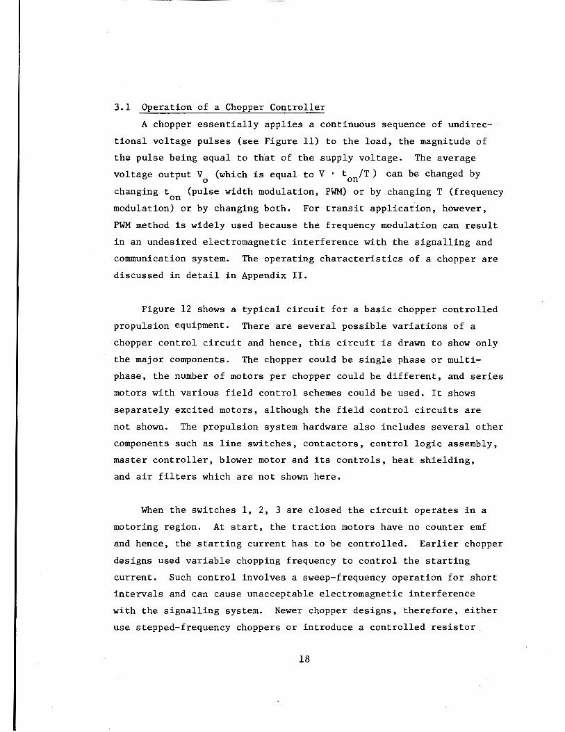
3.1 Operation of a Chopper Controller
A chopper essentially applies a continuous sequence of undirec
tional voltage pulses (see Figure 11) to the load, the magnitude of
the pulse being equal to that of the supply voltage. The average
voltage output V (which is equal to V • t /T) can be changed by o on changing t (pulse width modulation, PWM) or by changing T (frequency
on modulation) or by changing both. For transit application, however,
PWM method is widely used because the frequency modulation can result
in an undesired electromagnetic interference with the signalling and
communication system. The operating characteristics of a chopper are
discussed in detail in Appendix II.
Figure 12 shows a typical circuit for a basic chopper controlled
propulsion equipment. There are several possible variations of a
chopper control circuit and hence, this circuit is drawn to show only
the major components. The chopper could be single phase or multi
phase, the number of motors per chopper could be different, and series
motors with various field control schemes could be used. It shows
separately excited motors, although the field control circuits are
not shown. The propulsion system hardware also includes several other
components such as line switches, contactors, control logic assembly,
master controller, blower motor and its controls, heat shielding,
and air filters which are not shown here.
When the switches 1, 2, 3 are closed the circuit operates in a
motoring region. At start, the traction motors have no counter emf
and hence, the starting current has to be controlled. Earlier chopper
designs used variable chopping frequency to control the starting
current. Such control involves a sweep-frequency operation for short
intervals and can cause unacceptable electromagnetic interference
with the signalling system. Newer chopper designs, therefore, either
use stepped-frequency choppers or introduce a controlled resistor.
18

--- -C: 0
,I.I
I
- - - -
- - - -. C: 0
,I.I
- - - -
- - - -j
C: 0
,1.1·
L&J V) ..J ::::, a..
L&J CD c:( 1-..J 0 >
\ I I
I I I
I
I I
I
I
I I
I
I I
I 0
> >
39'dl10A
19
• +-'
--r 1--
I
--- --
1--
l
a: w Q. Q. 0 ::c 0 <C
..... ► ..... m W....1 a:o ::::, a: CJ t- z u.o
0 w CJ <C t....1 0 >

1
1 3 / L .... J l ...... J - & Dl & D2
CF N 0 .
4/ \...V '-V ~ y ~¾
T
1 I I /I
-
FIGURE 12 A CHOPPER CONTROLLER

in series during the start. Once the motors start and develop some
counter emf, one can eliminate the resistor (or the variable frequency
operation) and the motors can be directly controlled by choppers
Ch1 and Ch2 • These choppers can be operated with a phase difference
to give an effective multi-phase operation. Alternately one can use
two separate choppers, each controlling two motors on a truck. The
reactors 1 1 and 1 2 are used to improve load sharing between the motors
and the choppers.
Under regenerative braking conditions, the switch 3 is opened
and 4 is closed. The armature current I can now build up through a
a closed circuit - motors, choppers, and switch 4. After a sufficient
current builds up, choppers can be turned off. The reactors in the
circuit then tend to keep the armature current flowing, thereby
feeding the current back to the line through the free wheeling diodes
D1
and D2
• If the network cannot receive the current, it is directed
to a braking resistor RB by triggering the thyristor T.
3.2 (7-22) Deployment of Chopper Controllers
Chopper controlled transit equipment is being increasingly
introduced around the world. In addition to heavy rail vehicles, it
has also found application in light rail vehicles, street cars as
well as buses.
On the North American continent, chopper equipment was first
introduced on the BART (Bay Area Rapid Transit) system. Initially
250 cars (see Figure 13) were put in revenue service in 1972 and
200 cars were added during 1974-75 on the system. The cars registered
over 120 million miles in the first five years of revenue service.
This equipment was manufactured by Westinghouse Electric Corporation.
Chopper controlled propulsion equipment made by Garrett Corporation
was later introduced on the light rail system in Boston (MBTA) and
21

San Francisco (MUNI). Currently 275 of these propulsion units have been
delivered to the car builder. General Electric Company is currently
manufacturing chopper controlled propulsion equipment for revenue testing
in Chicago (10 cars) and New York (2 cars). MARTA in Atlanta has
ordered 100 cars for its new rapid transit system where revenue ser
vice is expected to start in July 1979. Propulsion equipment for
these cars using chopper control is being produced by Garrett.
Greater Cleveland Regional Transit Authority (GCRTA) has also ordered
48 chopper cars and its propulsion equipment will be made by Brown
Boveri. Toronto Transit Connnission (TTC) in Canada is buying 138 cars
(chopper propulsion equipment by Garrett Corporation) of which about
90 have already been delivered and are in operation to date. Toronto
will also be getting 200 light rail vehicles (CLRVs with chopper
equipment by Garrett Corporation) over the next few years. Similarly
Mexico City Metro has ordered 350 cars (using chopper equipment by
Mitsubishi Electric, Japan) which will be delivered over the next
few years. It can thus be seen that there are more than 1700 chopper
controlled cars in operation or on order in North America.
ASEA supplied four car-pairs of C7 type(lB) with chopper control
to Stockholm subway in 1973. Experience from revenue service has
shown that up to 35 percent of the supplied energy can be saved
depending on the line receptivity (ability of the line to receive
the braking energy). Encouraged by this experience the Stockholm sub
way ordered additional 20 cars in 1976. These chopper controlled
Cars (l9) oft C9 h . F. 14 Th .d h. h ype ares own in igure . ese can provi e ig
acceleration rates (1.3 m/s2
, 0.13 g, 2.9 mphps) and the regenerative
braking is available down to 2 km/h (1.25 mph). A typical thyristor
module consisting of a main thyristor, an auxiliary thyristor and
other relevant components is shown in Figure 15 and the complete
chopper equipment for the car is shown in Figure 16. The chopper
equipment package is roughly 5 feet wide and 11 feet long.
22

N (.;.)
& • -
~
' fiif f l f ti li:f ,; 1
" I '1 L ; i; 1,:;j ' ,,;~,o} I j I I I
FIGURE 13 BART CAR
j

FIGURE 14 SUBWAY CAR OF TYPE C9
FIGURE 15 A THYRISTOR MODULE
24
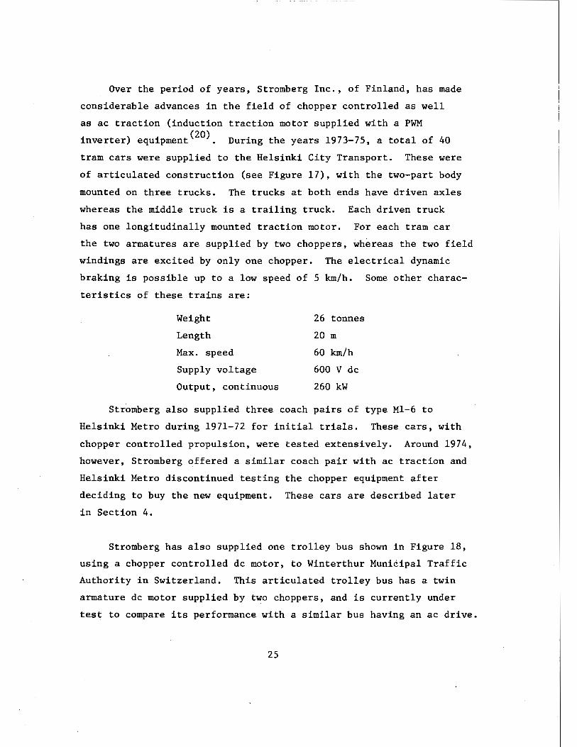
Over the period of years, Stromberg Inc., of Finland, has made
considerable advances in the field of chopper controlled as well
as ac traction (induction traction motor supplied with a PWM
inverter) equipment( 20). During the years 1973-75, a total of 40
tram cars were supplied to the Helsinki City Transport. These were
of articulated construction (see Figure 17), with the two-part body
mounted on three trucks. The trucks at both ends have driven axles
whereas the middle truck is a trailing truck. Each driven truck
has one longitudinally mounted traction motor. For each tram car
the two armatures are supplied by two choppers, whereas the two field
windings are excited by only one chopper. The electrical dynamic
braking is possible up to a low speed of 5 km/h. Some other charac
teristics of these trains are:
Weight
Length
Max. speed
Supply voltage
Output, continuous
26 tonnes
20 m
60 km/h
600 V de
260 kW
Stromberg also supplied three coach pairs of type Ml-6 to
Helsinki Metro during 1971-72 for initial trials. These cars, with
chopper controlled propulsion, were tested extensively. Around 1974,
however, Stromberg offered a similar coach pair with ac traction and
Helsinki Metro discontinued testing the chopper equipment after
deciding to buy the new equipment. These cars are described later
in Section 4.
Stromberg has also supplied one trolley bus shown in Figure 18,
using a chopper controlled de motor, to Winterthur Munieipal Traffic
Authority in Switzerland. This articulated trolley bus has a twin
armature de motor supplied by two choppers, and is currently under
test to compare its performance with a similar bus having an ac drive.
25

FIGURE 16 COMPLETE CHOPPER EQUIPMENT
FIGURE 17 ARTICULATED TRAMCAR
26

1,.", ,.j
FIGURE 18 TROLLEYBUS WITH CHOPPER CONTROL

Brown Boveri, Siemens and AEG-Telefunken are the three German
companies actively developing new propulsion equipment using de and
ac drives. Presently there are almost 200 cars with chopper control
in revenue service in Germany.
AEG, in collaboration with Siemens, supplied 28 units to
Wuppertal Suspension Railway-Monorail(2l) in 1973. As shown in
Figure 19 this is a two-car unit powered by 4 series wound de motors
rated 50 kW at 1700 rpm with a maximum speed rating of 3850 rpm. In
each car the two motors are connected in series and these in turn are
connected in parallel so that there is only one chopper for all the
four motors. Only dynamic braking is available.
The rapid transit streetcars made by AEG for Hanover are eight
axle articulated units with the two end trucks powered by individually
chopper controlled de traction motor rated at 218 kW at 1900 rpm.
Regenerative braking is used depending on the line receptivity, if
the voltage rises beyond allowable maximum dynamic braking is used.
Currently 100 units of this type are in regular operation for speeds
up to a maximum of 80 km/h. AEG has also supplied chopper controlled
tram cars to the city of Melbourne, Australia.
For heavy rail vehicles, AEG and Siemens have supplied chopper
controlled prototype equipment to Berlin and to the Munich Metro.
This equipment is still in operation since the past several years.
BBC also manufactures chopper controlled traction equipment.
Regenerative or dynamic braking is provided depending on the customer
requirements. BBC has considered two ways of using the kinetic energy
to heat the vehicle during braking. One way is to use dynamic braking
and distribute the heat lost in the braking resistor through the heat
ing system. This arrangement is very attractive where a new traction
28
system needs to be provided for an existing vehicle design. Another
way is to return the braking energy back to the line and separately
draw heating energy that can be better distributed by heating elements
along the vehicle. Such a system is in fact under consideration for
transit vehicles for Stuttgart area.
The Paris Metro (RATP) operating over 155 route miles, has more
than 900 rubber-tired cars and more than 1400 rail cars. Recently
RATP ordered 1000 new chopper controlled cars of MF 77 series shown
in Figure 20. First two cars were completed in October 1977 and the
first complete five-car trainset entered the service some time around . (22) April 1978 on Line 13 between St. Denis and Chantillon-Montrouge .
By mid-1979 all the trains on this line are expected to be of MF 77
stock. Subsequent deliveries will be for Lines 7 and 8.
The metro system of Lyons will run three-coach rubber-tired MU
equipment of Figure 21 with the possibility of adding a fourth coach
to the consist. The vehicle has monomotor trucks as shown in Fig
ure 22 and operates at a speed of 90 km/h. The braking energy cannot
be returned to the line, especially in the early morning and late at
night because the line is not receptive due to reduced traffic. This
energy is then used to feed the auxiliary power system. The
Marseilles Metro system is also expected to buy chopper controlled
equipment for their next buy.
The Sao Paulo metro system in Brazil ordered its first set of
198 chopper controlled cars in 1972, which were delivered in 1975.
The cars with traction equipment by Westinghouse have accumulated
over 33 million miles of revenue service. Since then, this metro
system has ordered 108 more carsets to be delivered over the two year
period 1978-79. Over the same period, 270 carsets with chopper con
trolled propulsion system will be delivered by Westinghouse to Rio de
Janeiro metro system in Brazil. 29

r-------------------------------------------- - -
FIGURE 19 WUPPERTAL SUSPENSION RAILWAY
FIGURE 20 MF77 CARS OF PARIS METRO
30
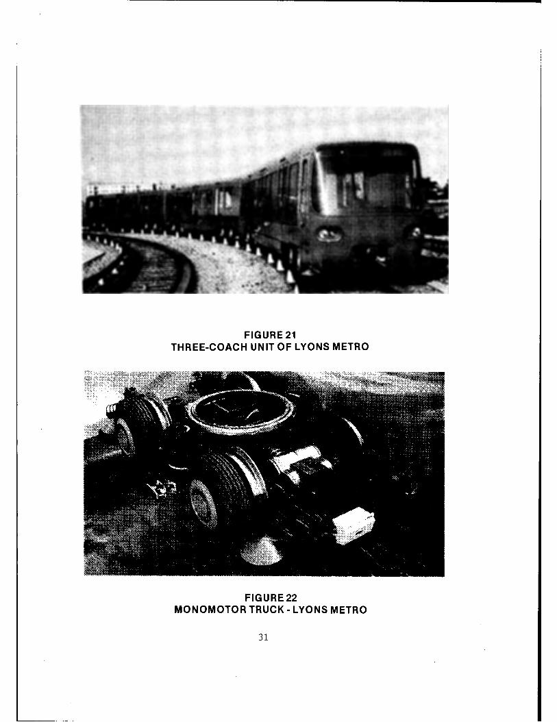
FIGURE 21 THREE-COACH UNIT OF LYONS METRO
FIGURE 22 MONOMOTOR TRUCK - LYONS METRO
31

In Japan the first prototype chopper equipment was produced in
the mid 1960's and several units were tested on Chiyoda, Ginza and
Hibiya Lines of Teito Rapid Transit Authority, Tokyo. Since then
choppers have been introduced on many transit systems such as in
Tokyo, Osaka, Sapporo, Nagoya, Kyoto. Currently about 350 cars with
chopper controllers by Mitsubishi Electric are in operation or on
order in Japan. Considering equipment by other Japanese companies it
can be estimated that there are probably more than 700 chopper cars in
operation or on order there.
3.3 Field Control of Traction Motors
If separately excited traction motors are used, a separate
chopper using thyristors or power transistors is usually used for field
control. If, however, a series motor is used, the field weakening
can be accomplished by using one of the several possible methods. One
can use a simple series/parallel connection of field windings which
gives a fixed 50% field weakening, or one can use shunt reactors in
parallel with the field or one can use additional field windings. The
time constant of the shunt reactor is usually adjusted such that there
is a proper division of current between the reactor and the field even
under transient and fault conditions. If an additional field winding
is used, it can be connected in the interrupting circuit of the arm
ature chopper to get a continuously varying field excitation for the
motor( 23 • 24). The main power circuit for this system, known as
Automatic Variable Field (AVF) system, is shown in Figure 23. The
field winding is divided into two sections: one winding F1
is connected
in series with the armature, while the other winding F2
is connected
in series with the free wheeling diodes DF1
and DF2
for motoring opera
tion. The two windings F1
and F2
are connected such that their fluxes
are cumulative. As the speed increases, the conduction ratio of the
chopper increases, thus reducing the "off" period. Since the field
F2
carries current during the "off" period, the effective field of the
32

I MOTORING
2
I BRAKING
FIGURE 23 AUTOMATIC VARIABLE FIELD CONTROL
33
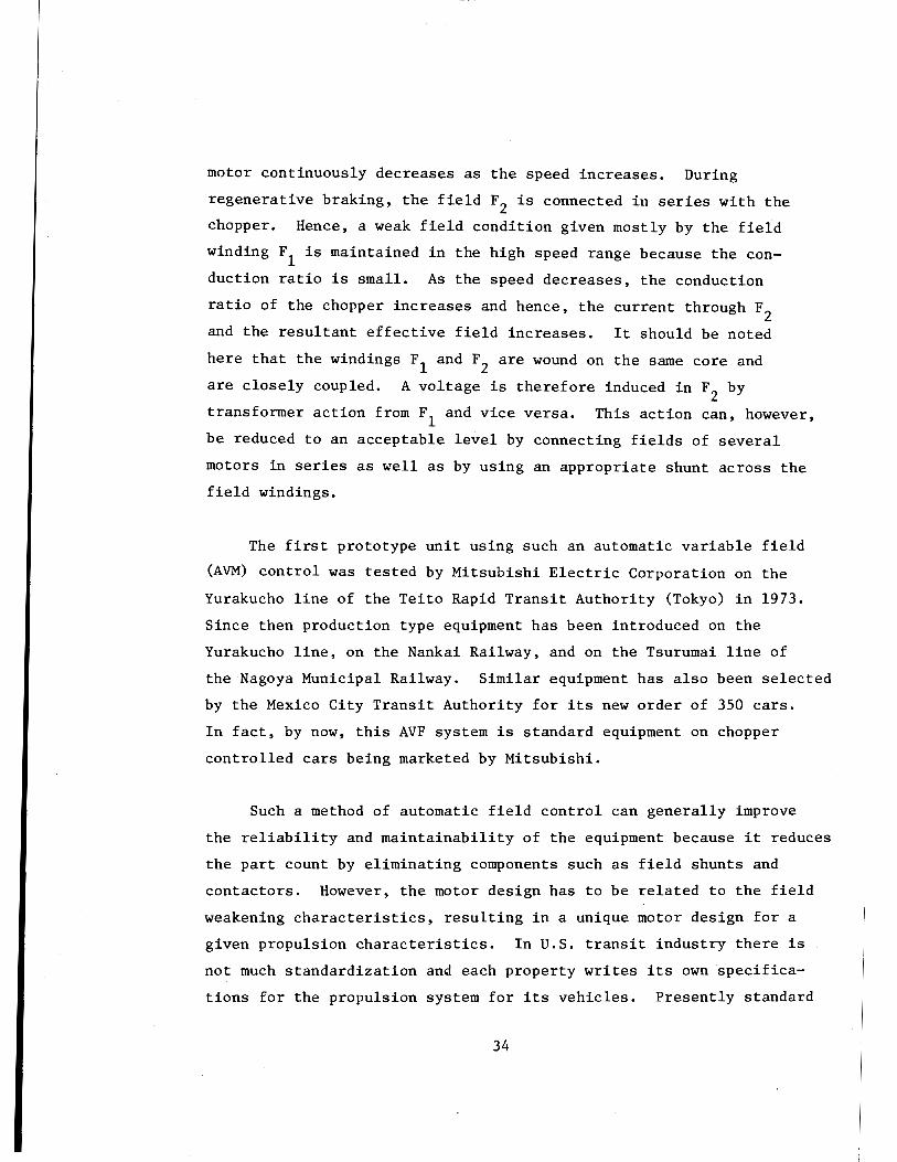
motor continuously decreases as the speed increases. During
regenerative braking, the field F2 is connected in series with the
chopper. Hence, a weak field condition given mostly by the field
winding F1 is maintained in the high speed range because the con
duction ratio is small. As the speed decreases, the conduction
ratio of the chopper increases and hence, the current through F2
and the resultant effective field increases. It should be noted
here that the windings F1
and F2
are wound on the same core and
are closely coupled. A voltage is therefore induced in F2
by
transformer action from F1
and vice versa. This action can, however,
be reduced to an acceptable level by connecting fields of several
motors in series as well as by using an appropriate shunt across the
field windings.
The first prototype unit using such an automatic variable field
(AVM) control was tested by Mitsubishi Electric Corporation on the
Yurakucho line of the Teito Rapid Transit Authority (Tokyo) in 1973.
Since then production type equipment has been introduced on the
Yurakucho line, on the Nankai Railway, and on the Tsurumai line of
the Nagoya Municipal Railway. Similar equipment has also been selected
by the Mexico City Transit Authority for its new order of 350 cars.
In fact, by now, this AVF system is standard equipment on chopper
controlled cars being marketed by Mitsubishi.
Such a method of automatic field control can generally improve
the reliability and maintainability of the equipment because it reduces
the part count by eliminating components such as field shunts and
contactors. However, the motor design has to be related to the field
weakening characteristics, resulting in a unique motor design for a
given propulsion characteristics. In U.S. transit industry there is
not much standardization and each property writes its own specifica
tions for the propulsion system for its vehicles. Presently standard
34
lines of traction motors are used for several applications and any
difference in propulsion system requirements is met by different
controller designs. It is, therefore, not clear if the application
of such an AVF system in U.S. can be economically justified at this
time. With increasing standardization in U.S. transit industry,
however, this type of field control would be of increasing value
in the future.
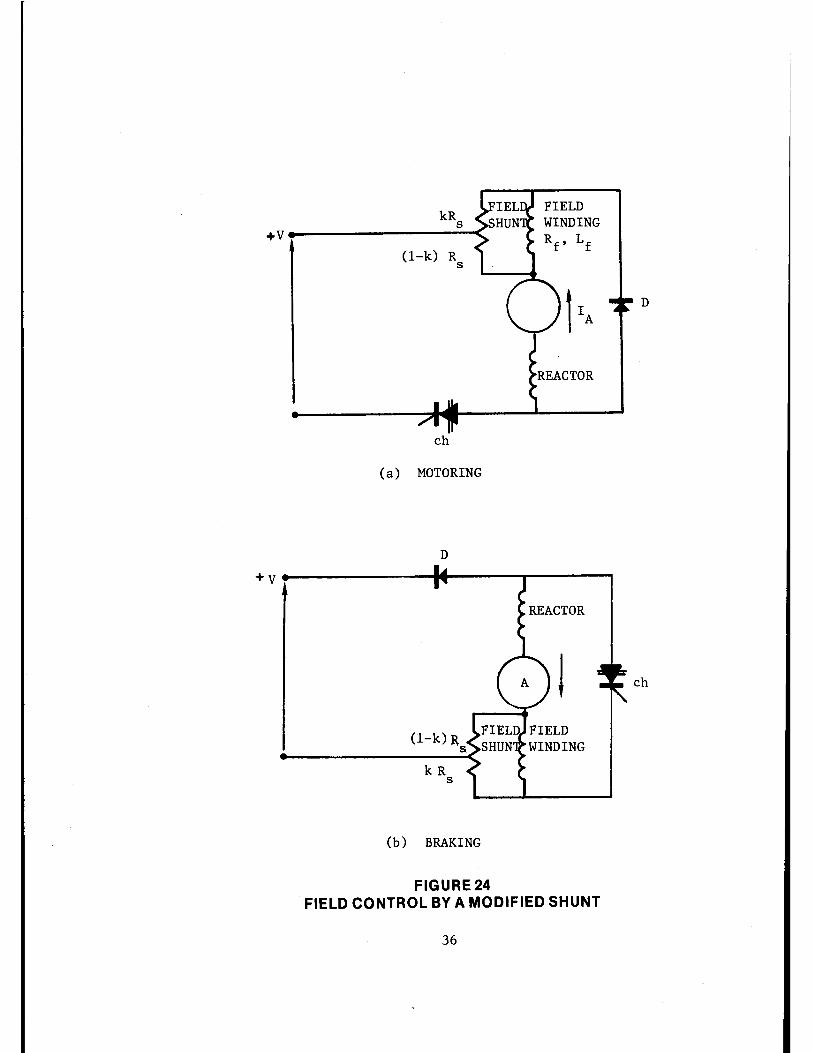
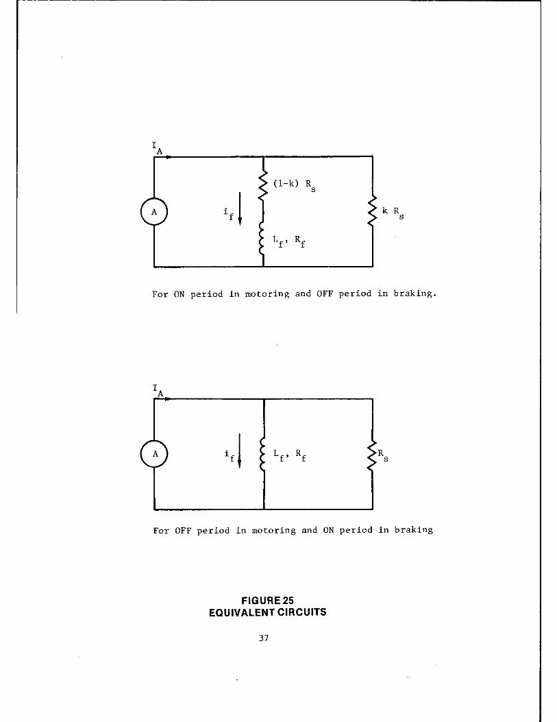
Another method of automatic field weakening of a series traction
motor can be illustrated with the help of Figure 24. A resistor is
connected in shunt with the series field winding and the power is
connected to a tap on this field shunt< 25 ). If the reactor in series
with the armature is sufficiently large, the armature current IA is
almost constant and one can obtain the equivalent circuits of Figure 25
for the operation during ON/OFF period for motoring/braking. The
instantaneous field current is thus a function of Kand the conduction
ratio a. The field current wave forms are of the type shown in
Figure 26 where the actual waveforms depend on the time constant
T = Lf/(Rf + Rs). The effective field weakening ratio is also a
function of Kand a as shown in Figure 27. At present Toshiba is
developing such a system for traction applications.
There are several other possible methods of obtaining field
control but a detailed discussion of these is beyond the scope of
this work.
3.4 Energy Savings by Regeneration
During the vehicle braking, the traction motors are used in
generating mode and convert the kinetic energy of the vehicle into
electrical form. In dynamic braking this energy is dissipated in
braking resistors while with regeneration at least a part of this
energy is returned to the line. Such a regeneration is inherently
35
kR s +v----------<
(1-k) R s
ch
(a) MOTORING
D
+v--------------------
(1-k) R s
kR s
(b) BRAKING
FIGURE 24
I
FIELD CONTROL BY A MODIFIED SHUNT
36
D
ch
(1-k) R s
k R s
For ON period in motoring and OFF period in braking.
R s
For OFF period in motoring and ON period in braking
FIGURE 25 EQUIVALENT CIRCUITS
37

0
-rand K constant
TIME
FIGURE26 FIELD CURRENT WAVEFORM
INCREASING K
CONDUCTION RATIO
FIGURE27 FIELD WEAKENING RATIO
38
INCREASING CONDUCTION RATIO a
1.0

possible with a chopper control. The magnitude of energy savings
possible for practical application, however, is widely misunderstood,
with numbers such as 50 percent energy savings often quoted. Although
these savings are possible under the most favorable conditions, the
actual energy savings are far below this figure.
There are several factors that limit the energy savings. The
most important of these is the fact that the total energy available
for regeneration is equal to the kinetic energy of the vehicle at the
moment the braking begins. This is further reduced by the energy
used in overcoming the train resistance and the losses of the motor
and associated circuits. The second factor is that full regeneration
may not be possible at high speeds when the motor voltage is higher
than the line voltage. Depending on the braking requirements, it may
be necessary to limit the current by external resistances and some
energy may be inevitably lost during the process. The third key
factor is related to the concept of line receptivity. This is a
measure of how much energy made available by regeneration can be
absorbed by the system. When the entire electrical system is con
sidered, there is a constant instantaneous energy balance between
the different sources and the sinks in the system. Line receptivity
is thus a dynamic factor depending on several system conditions
such as:
• Maximum voltage allowed onboard and on line
• Instantaneous power demand
• Substation characteristics
• Third rail impedance
• Regenerated power
All these factors vary widely and are almost never ideal at the same
time. Moreover, the actual duration of braking when regeneration is
possible and the duration of maximum power demand are very small com
pared to a typical vehicle run.
39

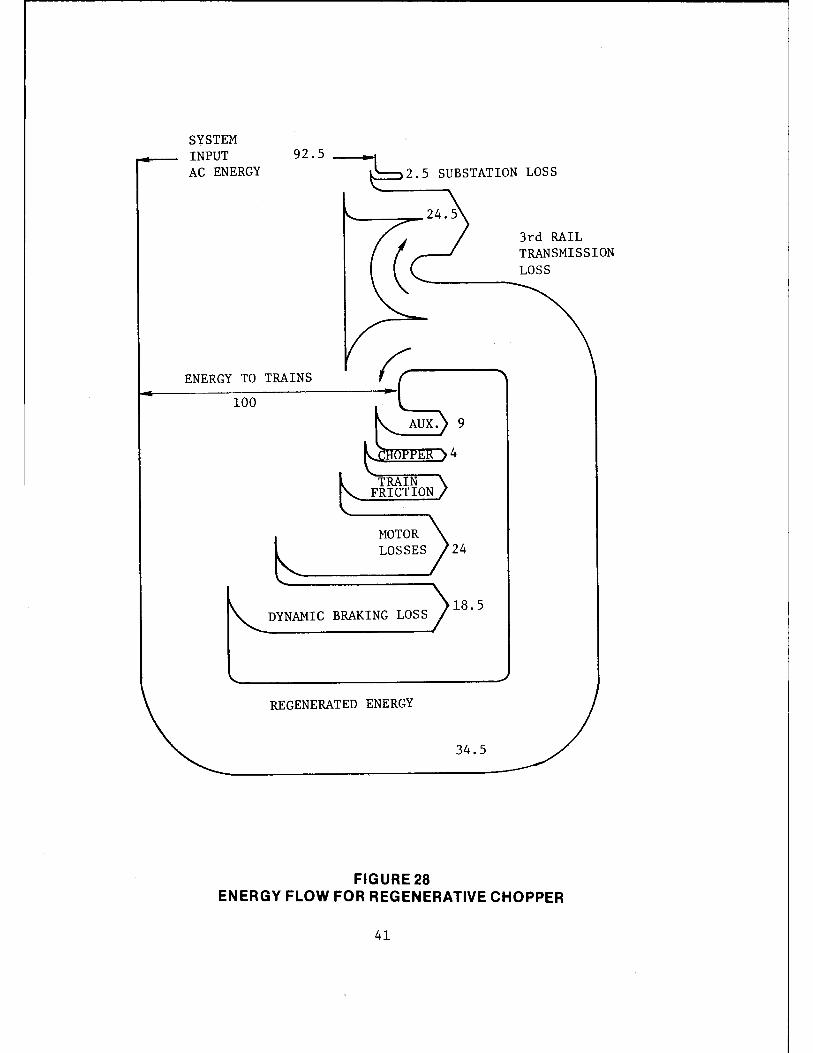
The actual energy saving possible on a typical rapid transit
system is thus limited to the order of 20 percent. This estimate is
also supported by the data obtained on the Sao Paulo Metro System in
Brazil(26 ). In the year 1977 the specific energy consumption was
reduced from about 4.2 kWh/car-km without regeneration to about
3.4 kWh/car-km with regeneration. Figure 28 shows the energy flow
with a regenerative chopper car for the NYCTA system simulation(S)
used previously (see Figure 9). As mentioned earlier, the actual
energy consumption in different components is highly dependent on
the duty cycle and these results are presented here primarily for
comparison.
3.5 Advanced Cooling Methods< 27 )
Thyristors, transistors and other electronic components require
cooling just as any other electrical apparatus. Oil cooling and
forced air cooling with a blower are two of the most common methods
of cooling choppers, inverters and other power electronic components.
In forced air cooling, outside air is first filtered and then forced
through the system, carrying heat away from heat sinks and other heat
dissipating components. One could also use a closed cycle system
where the same air is used again and again to cool the power electronics,
thereby eliminating possible contamination by dust and other unwanted
pollutants. However, for all such cooling systems, there are inevitable
maintenance and other operating costs associated with the blower, the
motor, the filter, etc.
Cooling systems using liquid freon offer great potential since
large amounts of heat energy can be dissipated without the use of a
pump. These systems were developed in the early 1970's for application
in intercity passenger equipment, wayside substation equipment and
general industrial equipment. In such a system, the heat generated
by semi-conductors is transferred to a refrigerant - liquid freon Rll3 -
40
SYSTEM INPUT 92.5 _ __. AC ENERGY 2.5 SUBSTATION LOSS
ENERGY TO TRAINS
100
TRAIN FRICTION
MOTOR LOSSES
DYNAMIC BRAKING LOSS
REGENERATED ENERGY
FIGURE 28
9
24
18.5
34.5
3rd RAIL TRANSMISSION LOSS
ENERGY FLOW FOR REGENERATIVE CHOPPER
41

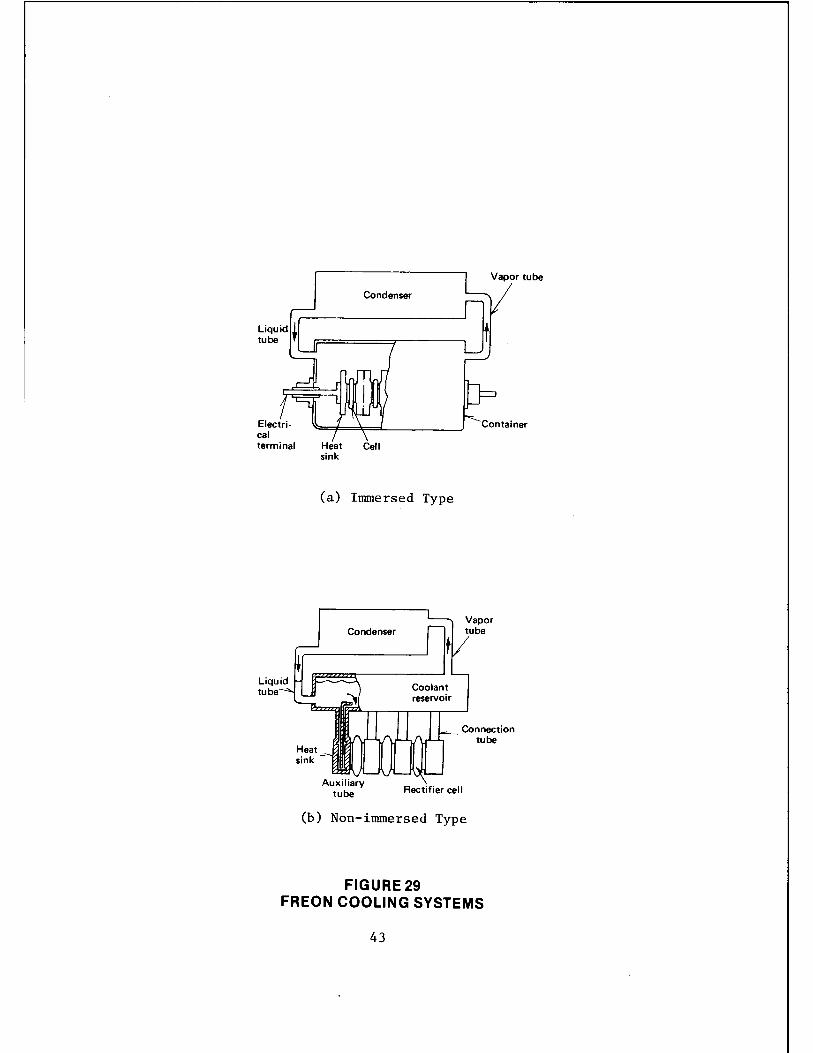
causing it to boil. The vapor thus formed passes to a condenser,
where it condenses and runs back under gravity to collect heat from
the semiconductors. The entire circulation is natural and no pump
is required. Two kinds of such systems are possible, as shown in
Figure 29. In an immersed type, the solid state equipment is immersed
in a bath of liquid freon and electrical connections are brought out
through insulated airtight terminals. In the non-immersed type, the
coolant flows from a reservoir through heat sinks and the solid state
components are directly accessible without disconnecting the cooling
system.
An effective cooling system is possible if the final temperature
of the refrigerant gives adequate heat transfer characteristics of
the heat sink within its permissible temperature range allowing for
the temperature difference between the heat sink and the actual semi
conductor junctions. The saturation or operating temperature of a
two-phase cooling system - utilizing a fluid in its liquid and vapor
form - is selected by considering the rate of heat generation and
the cooling capacity of the condenser. The vapor pressure required
within the system can then be obtained by knowing the properties of
the fluid. In any cooling system, a final temperature is attained
such that the heat generated by the equipment is equal to the heat
dissipated by the condenser at that temperature.
The transfer of heat from the heat sink to the coolant requires
that the surface of the heat sink be at a temperature somewhat greater
(~T) than the saturation temperature of the liquid. The relationship
between ~T and the heat transfer rate is highly nonlinear, as shown
in Figure 30. In the region B-C, nucleate boiling at the heat sink
surface, small changes in ~T create large changes in heat transfer
rate and this region offers very effective, stable cooling. Operation
at a greater ~Tis thermally unstable or less effective and hence avoided.
42
terminal
Heat sink
Heat sink
Cell
(a) Innnersed Type
Condenser
Container
Vapor tube
Connection tube
Rectifier cell
(b) Non-innnersed Type
FIGURE 29 FREON COOLING SYSTEMS
43

NUCLEATE BOILING
E
< i:,:i ~ < E-1 H
~ ~ -i:,:i ~ P-1 C/.l
i:.::1-E-1 O' ~: ~
0 i:,:i
H ~ C/.l
~ E-1
~ A
i:,:i ::c LOG (..1 T)
TEMPERATURE DIFFERENCE
FIGURE 30 HEAT TRANSFER CHARACTERISTICS
44

~-------------------------------------------
Such a freon cooling system has been in use on the Shinkansen
in Japan since 1972. As compared to forced air cooling, freon
cooling of a 1000 kW rectifier would reduce its weight by almost
50 percent and the volume by more than 65 percent. The first proto
type of such a system for urban rail vehicles was developed by
Mitsubishi and was tested in non-revenue service on the Chiyoda line
of Teito Rapid Transit Authority (Tokyo) in 1978. These tests were
quite satisfactory and revenue testing may be undertaken this year.
Alsthom (France) is also developing a freon cooling system for appli
cation in transit vehicles for Paris, Lyons and Marseilles.
3.6 Use of a Microprocessor
Chopper control of traction motors was introduced almost a decade
ago and improvements in the hardware have generally kept pace with
the state-of-the-art in power electronics as well as solid state logic
circuitry. Current chopper control circuits contain several analog
devices such as operational amplifiers, transistors, resistors,
capacitors and these are generally mounted on printed circuit boards.
These control systems are becoming increasingly complex because
additional functions - such as those required for diagnostics and
testing for example - are being introduced for the system to perform.
A propulsion control system regulates the systems as commanded
by the train line signals and by considering the status of all the
components. It has to control the armature and the field of all the
motors, limit the jerk, properly close and open the required contactors.
It has to sense several variables such as the line voltage, vehicle
speed and many others. In addition, it has to ensure the safety of
all components and shut down the system if necessary. These control
functions have to be designed individually for the specifications of
each specific propulsion system. Along with increasing complexity,
the reliability and maintainability requirements are also being
45

tightened and it is becoming more difficult to meet all these
severe performance envelopes.
Under these complex requirements the use of a microprocessor
in propulsion control can offer several potential benefits such as:
a. Improved reliability - Several components such as auxilliary relays and interlocks of different switches could be eliminated with microprocessor logic. This would result in a reduction of the part count and hence in improved reliability and reduced weight of equipment.
b. Hardware standardization - Standard hardware can be used for several applications with the microprocessor software providing the flexibility of design. This should have a system wide impact across the board such as reduced initial costs, improved reliability and maintainability, etc.
c. Integration of diagnostic and test capability - In addition to control of propulsion, the microprocessor can provide continuous monitoring of the system performance and suggest an operator action in case of system malfunction. The same microprocessor can be used as a diagnostic tool during trouble shooting, thus eliminating the need for separate computer-based diagnostic equipment.
Such microprocessor controlled chopper equipment for transit
cars has been developed and is currently marketed by Westinghouse
Electric Corporation of the U.S. and by Mitsubishi Electric of Japan.
After extensive development and testing in the laboratory environment,
prototype hardware was installed and operated on a transit car at
Sao Paul metro in revenue service. Based on the excellent results
of these trials, such microprocessor logic is included in the chopper
hardware for cars currently under manufacture for Rio de Janeiro
metro. Mitsubishi Electric developed and tested prototype equipment
with microprocessor control for a Dual Mode Bus and such an equip
ment has been developed for a transit car(ZS). This car will later
be tested in revenue service.
46
4.0 AC DRIVES USING INDUCTION MOTORS
An induction motor offers several important advantages over
the traditional de traction motor. These are:
• For a given motor volume, more space is available for electromagnetic structure and hence the motor has a high volume and weight power density.
• There are no sliprings, commutator and brushgear to maintain.
• The motor can be operated at higher voltage and at higher speed because of the absence of a commutator.
• The regenerative braking is inherent and no contactors are required to change over from motoring to braking.
• The steep speed-torque characteristics tend to prevent wheel slip.
• For a given horsepower per axle, a small, light motor permits a simple truck design.
These inherent advantages of using a three phase squirrel-cage
induction motor for traction were recognized long ago, but this
application could not gain ground until adequate control equipment
was available at an acceptable cost. The first research locomotive
using induction traction motor was the "Brush Hawk" developed by
Hawker Siddeley in 1965 but even then thyristor technology was not
sufficiently advanced and the inverter control required over 300
thyristors per megawatt of traction power. Recent advances in thyristor
technology have made it possible to reduce this number by a factor
of over 10.
The concept of controlling the speed of an induction motor for
traction application is discussed in detail in Appendix I and basic
operation of different kinds of inverters are discussed in Appendix II.
A brief history of ac drives for traction application will be given
here.
47
4 1 Ac D . f L . (29-37) • rives or ocomotives
Brown Boveri teamed up with Henschel to produce the first of the
three diesel electric prototypes of 2500 HP (hence the name DE 2500)
using an ac/dc/ac transmission in 1971. It was a 1840 kW, 80 tonne,
140 km/h locomotive with Co-Co axle arrangement. The other two DC 2500s
had similar ratings but one of them had Bo-Bo axle arrangement. These
units, shown in Figure 31, have been extensively tested on the Swiss
and German railway networks for different duties such as freight
service, passenger service up to 140 km/h, and shunting service at
speeds of 0-25 km/h. Two of these locomotives are in regular service
now with the German Railways.
One of the locomotives has been converted for all electric opera
tion by removing the diesel engine and the alternator and coupling it
to a 4-axle pilot car carrying the line-side power conversion equip
ment such as the transformer, power converters, filters, etc. This
unit of Figure 32 has been in operation since October 1974 and has
the following technical data:
Transformer primary voltage
Transformer secondary voltage
DC Link voltage
DC Link power, rated
Motor voltage
Power at wheels, rated
Motor frequency, maximum
Weight of locomotive
Weight of pilot car
Maximum speed
48
15 kV, 16 2/3 Hz, Single Phase
2 X 648 V
1300 V
1460 kW
1015 V/phase
~1300 kW
123 Hz
80 tonnes
54 tonnes
140 km/h

FIGURE 31 DE2500 LOCOMOTIVES WITH AC DRIVE
49

Brown Boveri has also supplied to Zechenbahn and Hafenbetrieb
Ruhr/Mitte AG (RAG) six dual frequency industrial locomotives of
the type shown in Figure 33, having the following ratings:
Power, continuous
Power, short time
Line voltage
Line frequency
Maximum speed
Weight
Axle arrangement
1.2 MW
1.5 MW
15 kV, Single Phase
15 2/3 Hz or 50 Hz
60 km/h
88 tonnes
Bo-Bo
Other locomotives by BBC also use induction motors - some under
development are Netherlands State Railway's test vehicle (1400 kW,
140 km/h, line voltage of 1500 Vdc, EDE 1000/500 industrial locomo
tives for 600 V de or diesel power and rated at 100 kW, Am 6/6 freight
and shunting locomotive of diesel-electric type as well as Ee 6/6
15 kV, 16 2/3 Hz electric locomotive for Swiss Federal Railways and
E120 Series of 5.6 MW, 160 km/h locomotives for German Federal Rail
ways. At present there are in all 37 units either in service or on
order with induction motor drive. Some of these units are shown in
Figure 34.
Russians have also been active in developing ac drives using
induction motors. An experimental system for VL80 series eight-axle
locomotive was built in 1968. The unit VL80K was one half locomo
tive(35) with 4 induction motors on 4 axles. Each motor had the
following rating:
Power - 1.2 MW
Voltage - 1200 V/phase
Maximum Speed - 1960 rpm
Frequency - 0-132 Hz
50

FIGURE 32 ALL ELECTRIC LOCOMOTIVE WITH AC DRIVE
FIGURE 33 DUAL FREQUENCY INDUSTRIAL LOCOMOTIVE
51

V, N
FIGURE 34 OTHER LOCOMOTIVES WITH AC DRIVE

The power circuit is shown in Figure 35. After initial investigations,
the Russians are now developing a full 8-axle VL80a locomotive. The
Russians have also awarded a contract to Stromberg of Helsinki, Finland,
to independently develop a competing propulsion system for the same
VL80a locomotive.
The National Railways of Finland, France and Italy are also
working on the development of ac drives for traction. Stromberg is
currently building a test locomotive for Finnish State Railways. It
will be a 4-axle locomotive with 1.2 MW per axle and is expected to
be completed by July 1979. The SNCF (France) conducted some experi
ments (1976) by putting a 500 kW induction motor on one axle of an
old locomotive and supplying it from a 600 kVA inverter( 35 ). A 1.2 MW
drive using an induction motor is currently under development by SNCF.
Italian State Railroads have built a shunting locomotive of Series
E 323 using an ac drive. This 3-axle locomotive is driven by a 280 kW
induction motor with a maximum speed of 3850 rpm at a frequency of
130 Hz.
4.2 Urban Vehicles
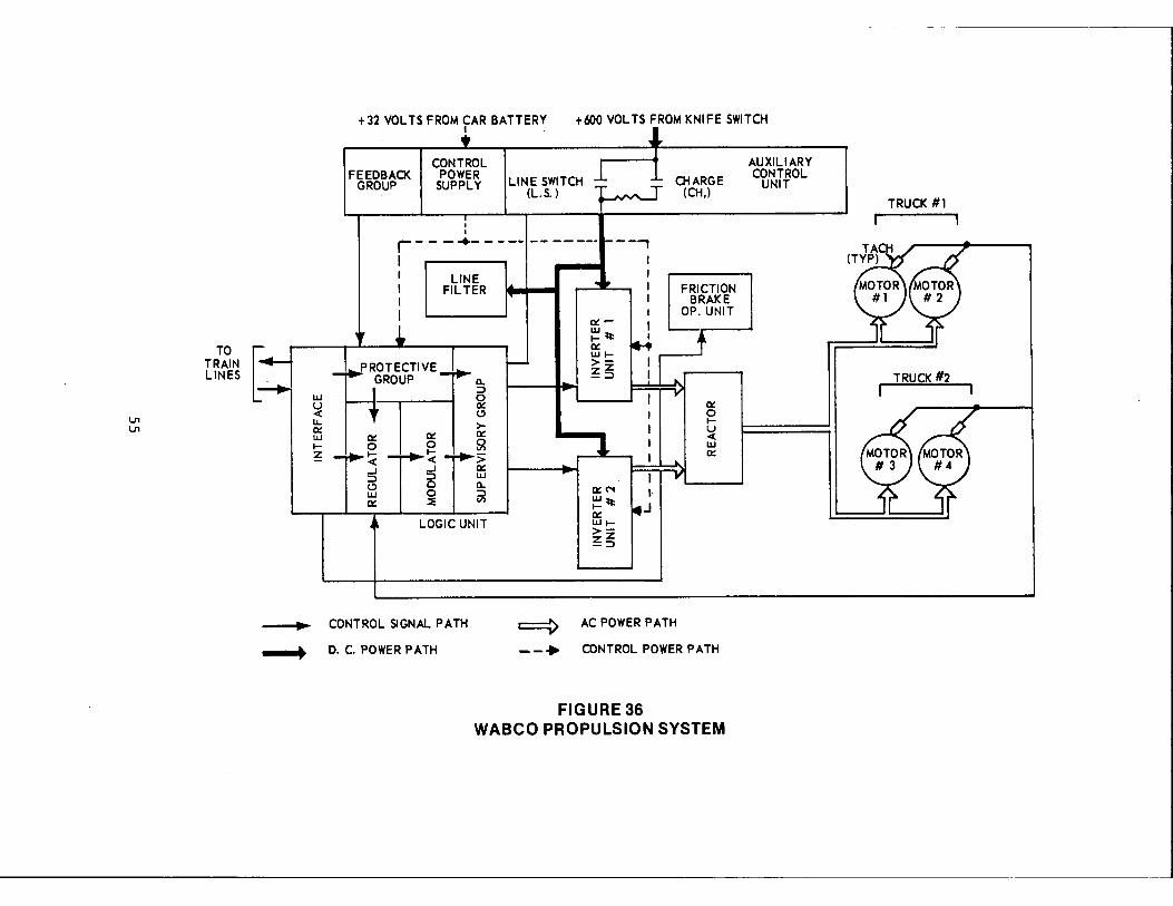
The first propulsion system using ac drive was tested on three
rapid transit cars on the Cleveland Transit System in 1972. The
propulsion equipment(38
) was developed by WABCO. The major components
of the system are shown in Figure 36. Two inverters supply all the
four motors through a paralleling reactor. The motors were four pole
motors with cast aluminum rotor and were self-ventilated. Each motor
contained a pulse-type tachometer for obtaining a speed feed-back signal.
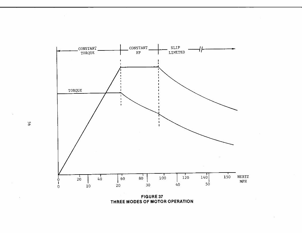
The three modes of motor operation in this WABCO system are
shown in Figure 37. They are as follows:
53

Vl ~
TRANSFORMER
~
~
~
DC/AC CONVERTERS
I I I
------------------'
FIGURE 35 POWER CIRCUIT OF VL80K
MOTORS
V, V,
+32 VOL TS FROM CAR BATTERY I
+600 VOL TS FROM KNIFE SWITCH
klNE SWITCH l 1 CHARGE
AUXILIARY CONTROL CONTROL FEEDBACK I POWER
UNIT GROUP SUPPLY I (L.S.) ~ (CH,)
I I I I r- - _ _.,_ - ---1-- -----..----,
I I
LINE I• I I 3E I I FRICTION FILTER I I
BRAKE OP. UNIT
ci:--
~~
T~N ~~ }.T,{ t: t I !i I ! I .. 1 I GROUP o.. LINES _ ::>
7 w 0
~ I Cl: u Cl: I 0 < ~ ... ~ ► I u Cl: Cl: Cl: < w ~ I w ... 0
Cl:
~ --~ T~ > ..J ..J Cl: ::> ::> w ~ 0 0..
I Q:N
~~-w O ~ ~~ Cl: :IE Cl:
LOGIC UNIT WI->-zZ -::>
---IIIIP► CONTROL SIGNAL PATH ~ AC POWER PATH
.._. D. C. POWER PATH - -♦ CONTROL POWER PATH
FIGURE 36 WABCO PROPULSION SYSTEM
I TRUCK #1
11 TRUCK_ #_2
\J1 0\
_____ CONSTANT I CONSTANT-+- SLIP __ _,,,__ _____ _
I
0 I 0
TORQUE HP LIMITED
TORQUE
20 I 4o
10
60 80 100 120
20 30 40
FIGURE 37 THREE MODES OF MOTOR OPERATION
50
150 HERTZ MPH

a. Constant torque - 1-60 Hz operation for 0-22 mph where the motor is operated at constant slip and constant airgap flux. This done by keeping the ratio V/f constant (after making an allowance for IR drop).
b. Constant horsepower - At some frequency the inverter reaches a voltage limit and if the frequency is increased further, the airgap flux decreases in inverse proportion with the frequency. It is necessary to increase the operating slip to maintain the motor current. This is possible only for slips up to a maximum value which in this case was 3 percent. This operation was for 60-95 Hz and 22-35 mph.
c. Slip limited - Once a maximum slip is reached at 95 Hz and 35 mph, the airgap flux, current, and hence the torque, are allowed to drop.
Regenerative braking was possible for speeds down to 5 mph and
a voltage limiting circuit prevented the voltage from exceeding the
prescribed maximum. The entire braking control was done without any
contactors. In case of non-receptive line, friction braking was
used to meet the requested braking rate. On the average, energy
savings by regeneration amounted to 29% on the test car( 3S).
Each motor was rated at 110 kW with a maximum speed of 4500 rpm
at 150 Hz. Each inverter was rated 350 kVA. Over a period of three
years the three cars ran about 130,000 car-km. This test program
demonstrated that an ac drive with induction motor can meet all the
functional requirements for a rapid transit rail car with possibilities
of regeneration.
As mentioned earlier, Stromberg had supplied three chopper con
trolled coach-pairs Ml-6 to Helsinki Metro during 1971-72 for initial
trials (construction of Helsinki Metro began in 1969 and the first
line, 11 km long, between Kamppi and Puotinharju will be completed
in 1981). Around 1974, however, Stromberg offered a similar coach
pair using induction motor drive< 39). After careful deliberations
57
Helsinki Metro ordered three coach-pairs of series MlOO of Figure 38
with an ac drive. Thus by mid-1976 Helsinki Metro was able to test
both types of coach-pairs, one with the de drive and the other with
an ac drive. As a result of these trails, the Helsinki Metro chose
ac induction motor drive for their transit cars and Stromberg is
currently manufacturing 42 coach-pairs of series MlOO for delivery
over 1977-84.
In the ac induction motor drive, each truck of the train has two
induction motors connected in parallel supplied by a PWM inverter as
shown in Figure 39. Thus each coach-pair has 4 inverters and 8
traction motors. The wheel diameter is 800 mm± 3 mm and there is no
slip control since the motors are in parallel and supplied with a
common inverter. Some other characteristics of these sets are as
follows:
Weight
Length
Maximum speed
Supply voltage
Output, continuous
Motor weight/output
Motor speed, rated
31 tonnes/coach
21.5 m/coach
90 km/h
750 V de
500 kW/coach
500 kg/125 kW
1,990 rpm at 68 Hz
The inverter characteristics for MlOO coach are:
Input voltage 750 V de
Output voltage 560 V ac, 3 phase
Rated output 300 kVA
Frequency 0-130 Hz
Weight 660 kg
Dimensions 1,600 X 875 X 610 mm
58

A-coach t I 1
R
FIGURE 38 A COACH-PAIR OF SERIES M100
750V -
R
FIGURE 39 THE MAIN CIRCUIT OF M100
59
8-coach T
R R
In 1977, Stromberg supplied a trolleybus using an inverter
controlled induction motor to Winterthur Muncipal Traffic Authority
in Switzerland(ZO). This articulated trolleybus has one induction
motor driven by one inverter. Some of the characteristics of this bus
are as follows:
Trolleybus
Length
Width
Weight
Max. speed
Supply voltage
Brakes
17.8 m
2.5 m
15 tonnes
60 km/h
600 V de
eddy current and air brake
A similar trolley bus using ac drive and regenerative braking is
currently under development for City of Helsinki and is scheduled
to be tested beginning early this year.
AEG Telefunken, West Berlin is also developing ac drive systems
using induction motors driven by PWM inverters for urban vehicles.
Over the years they have investigated, and also tested in part,
several alternate systems such as ac or de supply, voltage or current
drive, two quadrant or four quadrant controllers(40). From this
experience, AEG has built a prototype urban vehicle of Figure 40
which is being tested at present under operating conditions on
Berlin Metro (BVG)( 4i-43). This is a two car unit of F-76 series
with an ac drive instead of a conventional camshaft controlled de
drive.
This two-car unit has eight induction motors driving eight axles
and all these motors are connected in parallel controlled by a single
inverter (see Figure 41). During braking extra resistances are
60
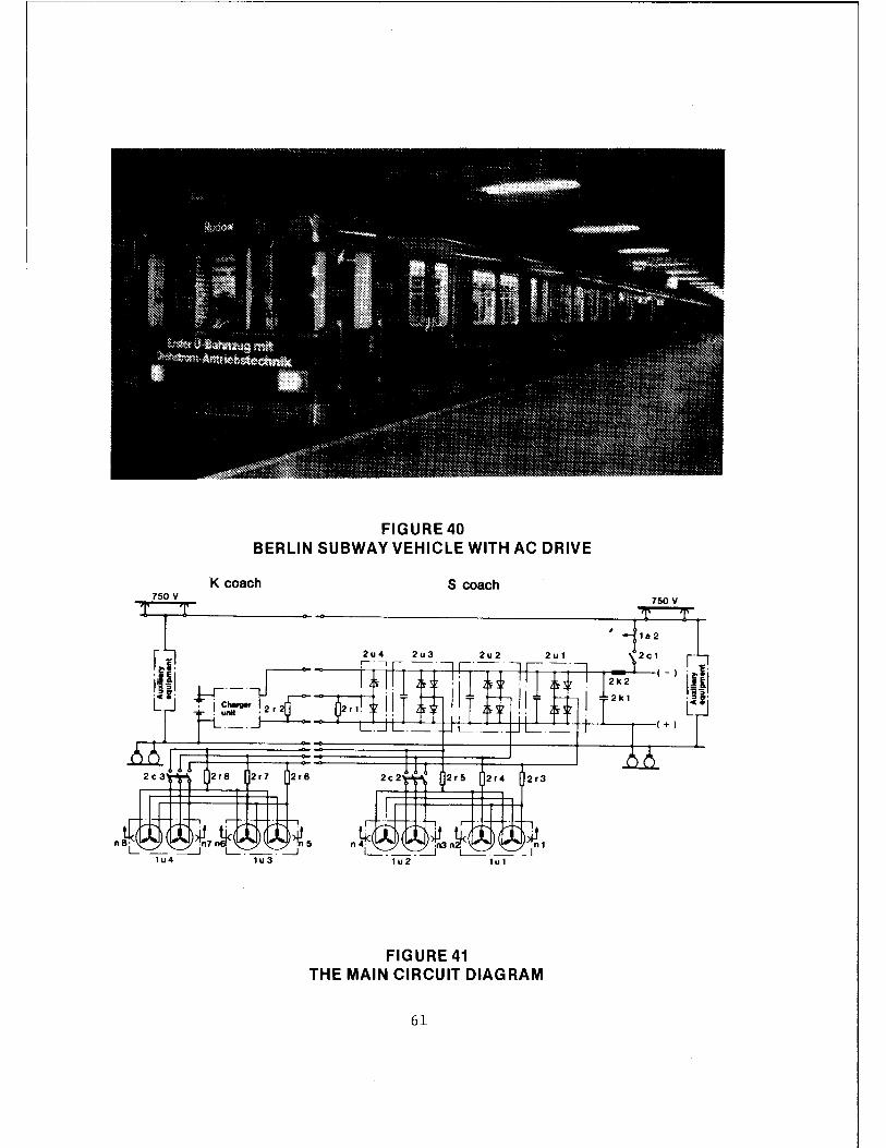
FIGURE 40 BERLIN SUBWAY VEHICLE WITH AC DRIVE
K coach S coach
2c3 2r8 2r7 2r6 2r5 2r4 2r3
FIGURE 41 THE MAIN CIRCUIT DIAGRAM
61
connected in series with the motors so that the inverter needs only
to be designed for motoring and not for the peak braking power.
This inverter has a nominal rating of 775 kVA at 560 V and 940 kVA
at a maximum allowable line voltage of 900 V. Each truck has a
two-motor unit as shown in Figure 42 where each motor drives one of
the two axles through a bevel gear. Both the axles are thus not
rigidly coupled, allowing for larger differences in the wheel
diameters in a truck. The motor is of a special high slip design
to improve load sharing. After initial testing, this vehicle has
been in regular service since January 1978 of Line 9 of BVG. The
individual traction motor is rated as follows:
Power 70 kW
Current 92 A
Voltage 560 V
Frequency 60 Hz
Speed 1153 rpm
Weight of the twin motor 1035 kg
The Berlin Metro-BVG is currently buying camshaft control equip
ment for their F76 series and their next expansion is expected to be
in 1982. AEG will probably sell 3-6 car pairs for a new pre-series
sone time around 1980 and they expect BVG to select ac traction for
the next order.
BBC is also currently developing a new traction system using
induction motor drive for Hamburg Transit Authority. This will be a
three-coach articulated vehicle with four two-axle trucks. The three
axles on each end are driven by a total of six induction traction
motors and will be powered by two inverters one in each of the end
ears. A prototype is expected to be ready for the international
exhibition in Hamburg 1979.
62
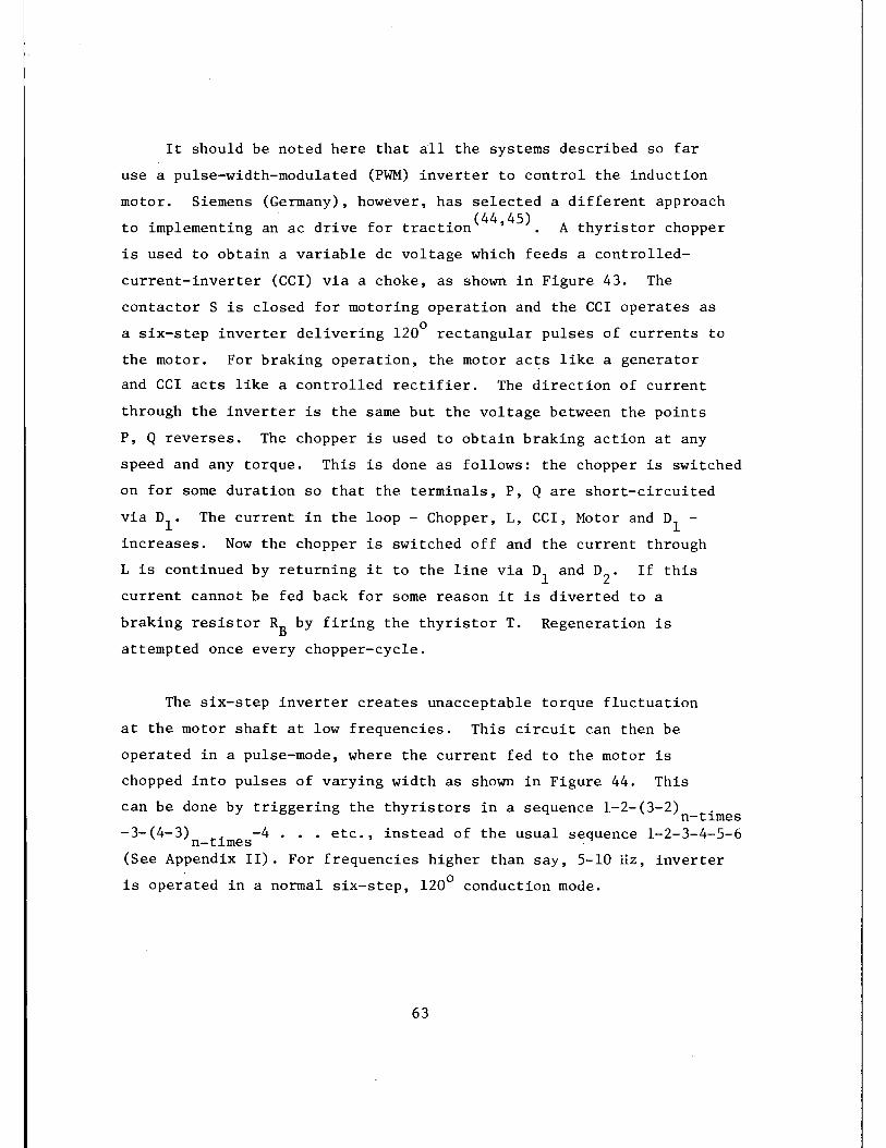
It should be noted here that all the systems described so far
use a pulse-width-modulated (PWM) inverter to control the induction
motor. Siemens (Germany), however, has selected a different approach
to implementing an ac drive for traction( 44 , 45 ). A thyristor chopper
is used to obtain a variable de voltage which feeds a controlled
current-inverter (CCI) via a choke, as shown in Figure 43. The
contactor Sis closed for motoring operation and the CCI operates as
a six-step inverter delivering 120° rectangular pulses of currents to
the motor. For braking operation, the motor acts like a generator
and CCI acts like a controlled rectifier. The direction of current
through the inverter is the same but the voltage between the points
P, Q reverses. The chopper is used to obtain braking action at any
speed and any torque. This is done as follows: the chopper is switched
on for some duration so that the terminals, P, Qare short-circuited
via n1 • The current in the loop - Chopper, L, CCI, Motor and n1
-
increases. Now the chopper is switched off and the current through
Lis continued by returning it to the line via n1
and D2
. If this
current cannot be fed back for some reason it is diverted to a
braking resistor RB by firing the thyristor T. Regeneration is
attempted once every chopper-cycle.
The six-step inverter creates unacceptable torque fluctuation
at the motor shaft at low frequencies. This circuit can then be
operated in a pulse-mode, where the current fed to the motor is
chopped into pulses of varying width as shown in Figure 44. This
can be done by triggering the thyristors in a sequence 1-2-(3-2) . n-times -3-(4-3) . -4 ... etc., instead of the usual sequence 1-2-3-4-5-6 n-times (See Appendix II). For frequencies higher than say, 5-10 Hz, inverter
is oper~ted in a normal six-step, 120° conduction mode.
63
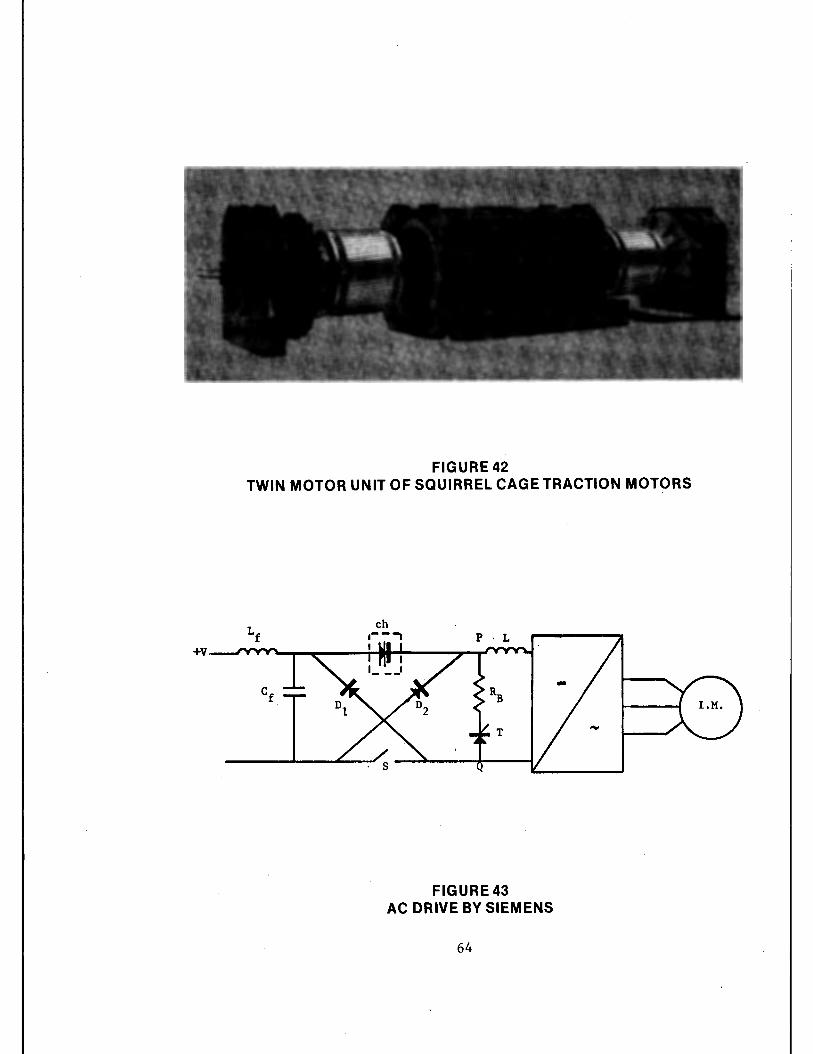
FIGURE 42 TWIN MOTOR UNIT OF SQUIRREL CAGE TRACTION MOTORS
FIGURE 43 AC DRIVE BY SIEMENS
64
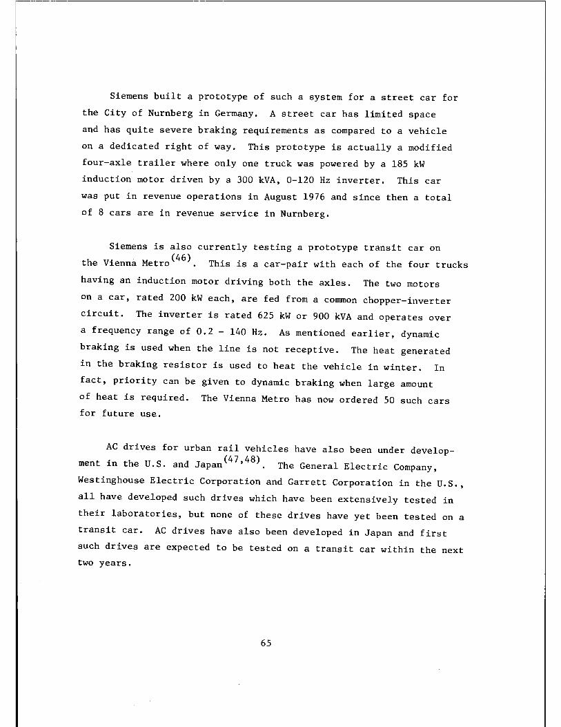
Siemens built a prototype of such a system for a street car for
the City of Nurnberg in Germany. A street car has limited space
and has quite severe braking requirements as compared to a vehicle
on a dedicated right of way. This prototype is actually a modified
four-axle trailer where only one truck was powered by a 185 kW
induction motor driven by a 300 kVA, 0-120 Hz inverter. This car
was put in revenue operations in August 1976 and since then a total
of 8 cars are in revenue service in Nurnberg.
Siemens is also currently testing a prototype transit car on
the Vienna Metro(46
). This is a car-pair with each of the four trucks
having an induction motor driving both the axles. The two motors
on a car, rated 200 kW each, are fed from a common chopper-inverter
circuit. The inverter is rated 625 kW or 900 kVA and operates over
a frequency range of 0.2 - 140 Hz. As mentioned earlier, dynamic
braking is used when the line is not receptive. The heat generated
in the braking resistor is used to heat the vehicle in winter. In
fact, priority can be given to dynamic braking when large amount
of heat is required. The Vienna Metro has now ordered 50 such cars
for future use.
AC drives for urban rail vehicles have also been under develop
ment in the U.S. and Japan(47 , 4B). The General Electric Company,
Westinghouse Electric Corporation and Garrett Corporation in the U.S.,
all have developed such drives which have been extensively tested in
their laboratories, but none of these drives have yet been tested on a
transit car. AC drives have also been developed in Japan and first
such drives are expected to be tested on a transit car within the next
two years.
65
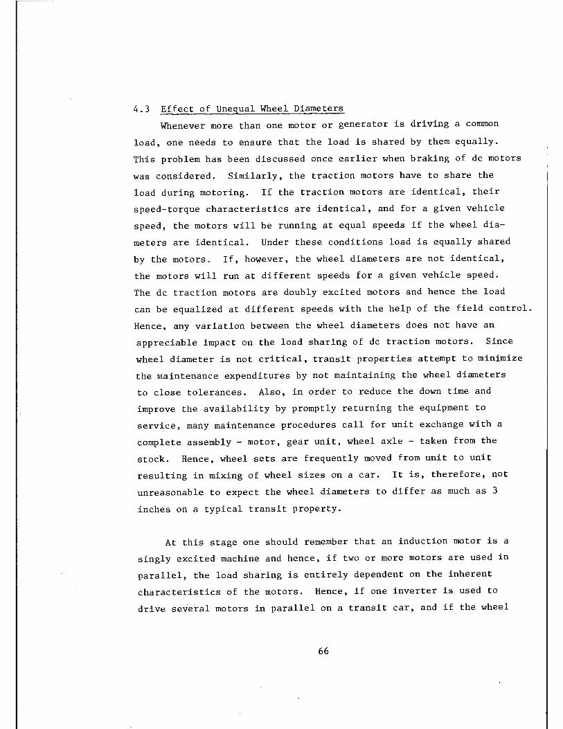
4.3 Effect of Unequal Wheel Diameters
Whenever more than one motor or generator is driving a connnon
load, one needs to ensure that the load is shared by them equally.
This problem has been discussed once earlier when braking of de motors
was considered. Similarly, the traction motors have to share the
load during motoring. If the traction motors are identical, their
speed-torque characteristics are identical, and for a given vehicle
speed, the motors will be running at equal speeds if the wheel dia
meters are identical. Under these conditions load is equally shared
by the motors. If, however, the wheel diameters are not identical,
the motors will run at different speeds for a given vehicle speed.
The de traction motors are doubly excited motors and hence the load
can be equalized at different speeds with the help of the field control.
Hence, any variation between the wheel diameters does not have an
appreciable impact on the load sharing of de traction motors. Since
wheel diameter is not critical, transit properties attempt to minimize
the maintenance expenditures by not maintaining the wheel diameters
to close tolerances. Also, in order to reduce the down time and
improve the availability by promptly returning the equipment to
service, many maintenance procedures call for unit exchange with a
complete assembly - motor, gear unit, wheel axle - taken from the
stock. Hence, wheel sets are frequently moved from unit to unit
resulting in mixing of wheel sizes on a car. It is, therefore, not
unreasonable to expect the wheel diameters to differ as much as 3
inches on a typical transit property.
At this stage one should remember that an induction motor is a
singly excited machine and hence, if two or more motors are used in
parallel, the load sharing is entirely dependent on the inherent
characteristics of the motors. Hence, if one inverter is used to
drive several motors in parallel on a transit car, and if the wheel
66

diameters are not identical, the motors will not share the load
equally and this could pose a serious problem with large difference
in wheel diameters.
Figure 45 shows a typical slip-torque characteristics of an
induction motor. For a given vehicle speed, the motor driving the
axle with large wheels will operate with lower speed. This means it
will operate at higher slips while motoring and hence will draw more
current and supply more torque. In braking region, however, the same
motor will operate at lower slip and hence will be loaded lightly.
So if motoring and braking periods are somewhat equal, the thermal
load on all motors is not highly unbalanced, although the motors will
need to have some additional thermal capacity. Furthermore, adhesion
problems may result from mismatched wheel diameters. In motoring,
the more highly loaded axle with larger wheels will tend to slip;
in braking the more highly loaded axles with smaller wheels will tend
to slide. In either case the actual slipping or sliding will be self
correcting, producing an intermittant rolling/slipping or sliding
action. Any accelerated wear from this action will, over the long
term, be self-correcting for slipping during motoring but worsen the
situation for sliding during braking.
The sensitivity of load sharing to wheel diameters can be
reduced if high slip motors are used because for these motors with
higher rotor resistance, variation of torque for a given change in
slip is smaller. These high slip motors are, however, inefficient
and hence bigger and heavier.
European and Japanese transit properties maintain the wheel
diameters to close tolerances - within 3-10 mms (< 1/2 inch). This
is not done in the U.S. and, as mentioned earlier, very often differ
ences as large as 3" are found. If ac traction is used in the U.S.,
67
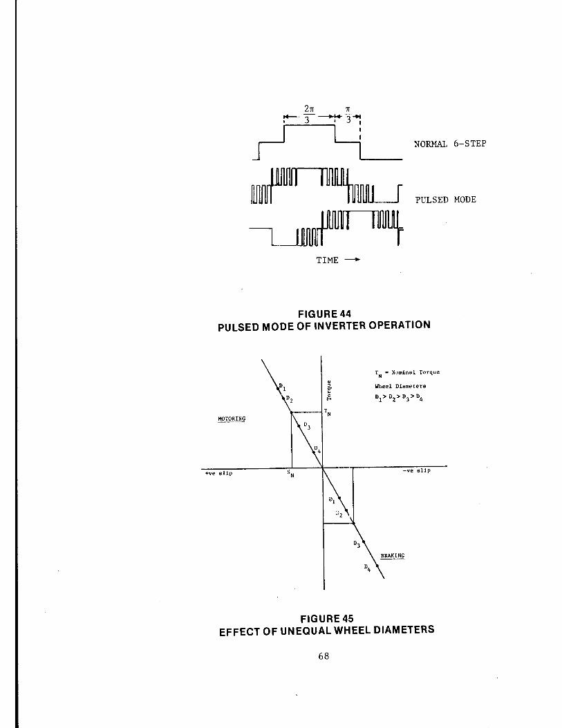
2TT TT ---3 --.... -3 .... I I I
TIME --
FIGURE 44
NORMAL 6-STEP
PULSED MODE
PULSED MODE OF INVERTER OPERATION
TN• Nominal Torque
Wheel Diameters
+ve slip -ve slip
FIGURE 45 EFFECT OF UNEQUAL WHEEL DIAMETERS
68

it is generally agreed that the wheel diameters will have to be main
tained much better than that - within say at least 3/4-1 1/4 inch.
However, a final choice cannot be made until practical limit of
adhesion considerations are experimentally determined.
69

5.0 AN AC DRIVE WITH A SYNCHRONOUS MOTOR
The synchronous motor can be advantageously used in place of the
de motor for various applications including vehicle traction. For
variable speed applications, the synchronous motor has to be supplied
from a variable voltage-variable frequency (VVVF)source. The speed
of the motor can be controlled by varying the frequency, whereas the
torque of the motor can be controlled by varying the airgap flux in
the motor. The principle of such a control is very similar to that
for an induction motor. However, doubly fed synchronous motors can
operate at leading power factors when overexcited and this has enormous
implications in the design of the inverters and/or cycloconverters
used to control these motors. The different types of synchronous
motors are discussed in Appendix I. The state of the art of such
drives will be described here.
5.1 A Self-Synchronous Propulsion System
A development of a self-synchronous system was undertaken
(October 1975) under the Advanced Subsystem Development Program (ASDP)
sponsored by the DOT/UMTA. Delco Electronics was the contractor.
Th . 1 · ( 49- 52 ) · h · 11 h . p· 46 is propu sion system is sc ematica y sown in igure .
The 600 V de supply is converted to a high frequency ac voltage with
a frequency of 350-1200 Hz. This voltage is then converted to a low
frequency ac by means of a cycloconverter. The output of the cyclo
converter with a maximum frequency of 200 Hz, is directly connected
to the stator of the motor. The rotor field winding of the motor is
supplied from a rotating transformer and a rotating rectifier placed
on the shaft of the motor. The primary of the rotating transformer
is excited by a current transformer having its primary windings in
series with the cycloconverter. With a rotor position feedback, the
characteristics of such a system are almost identical with those of
a de series motor. The motor and the associated control are oil cooled
to obtain high power density. Dynamic and/or regenerative braking is
70
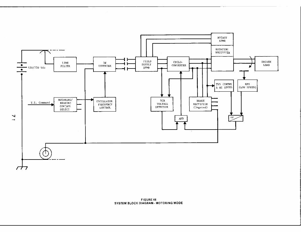
ROTARY XFMR
----- ROTATING /' RECTIFIER
---It-- - ' -- LINE 311 FIELD T - --t t-- - CYCLO- DRIVEN
• FILTER INVERTER SUPPLY CONVERTER " - 450/750 Vdc ---I t-- XFMR LOAD
• - ----I .,j~ .n T
~ TVS (INTMT RPS & HI SPEED (LOW SPEED)
,, ,r MOTORING/ ~ -
T.E. Command~ ~ OSCILLATOR SCR BRAKE
BRAKING -~ - FREQUENCY VOLTAGE RECTIFIER
CONTROL -SELECT - CONTROL DETECTOR (Un gated) -
1~ '. ....... I AND l l~I t f I
(ct) -----
-'
FIGURE46 SYSTEM BLOCK DIAGRAM - MOTORING MODE

available and is controlled by means of a separate solid state con
verter and a two-stage braking resistor switched in and out by means
of a thyristor.
5.2 Propulsion System Specifications
The propulsion system was designed to meet the following per-. (50 51)
formance requirements: '
a. Transit Route Performance
• For the conditions of a nominal wheel diameter of 30" and no wind, the energy consumption for a round-trip over the synthetic test route at the Transportation Test Center shall not exceed 10.2 kWh/car-mile without regeneration. With regeneration to a fully receptive line, this consumption shall not exceed 6.4 kWh/car-mile.
• The total round trip time for the above 18.5 mile distance shall not exceed 39 minutes.
b. Discrete Performance Requirements
• The railcar shall be able to maintain a speed of 80 mph with a wheel diameter between 28-30 inches on a level tangent track without wind.
• The car shall maintain 80 mph intermittently on a level tangent track with a 15 mph headwind.
• The car shall maintain a speed of 70 mph on a 3 percent grade for a distance of 6000 feet.
• The car shall meet the following acceleration specification
3.0 ± 0.2 mphps to 25 mph travel 700 feet in 20 secs from stop accelerate from Oto 60 mph in less than 38 secs
• Dynamic braking alone should be capable of providing deceleration of - 3.0 ± 0.2 mphps from 80 mph to 10 mph on level track without wind.
• Regenerative braking shall be available from 80 mph to 25 mph.
• Jerk rate shall not exceed 2 mphpsps
72

• The maximum capability of the cooling system shall be based onthe following duty cycle repeated over a period of 30 minutes
a full power acceleration to 80 mph followed immediately by full dynamic braking to a full stop and a rest period of 20 secs.
5.3 System Components
The propulsion system consists of the following major components(5l).
• Line Filter: The line filter consists of a dual inductor and two capacitor banks at the input of two power converters for the two drive systems per car as is shown in Figure 47. The nominal circuit constants for this filter are an inductance of 2.5 mH and a capacitance of 17600 µF. This gives a resonant frequency of 25 Hz and a resonant impedance of 0.377 ohm. The damping resistor R is adjusted to give a damping of 0.4 with the motor drives de-energized. The dual inductor assembly, shown schematically in Figure 48, consists of two parallel windings on two separate E-cores which share a commom I-section. The damping is obtained by putting a metal sheet in the airgap. The material and the dimensions of this sheet were empirically determined to obtain a desired damping response.
• Inverter: The inverter is a series inverter as shown in Figure 49. The inductors are 150 µH each with Q of 180 in free space at 1000 Hz. The capacitors are liquid cooled of a type developed for use by induction heating industry. Each of the capacitors contains two 20 µF and two 40 µF sections as shown in Figure 50(a). The equivalent circuit of this connection is shown in Figure 50(b). The 80 µF segments are coupling capacitors whereas 40 µF segments are commutating capacitors. The power semiconductors, inductors and capacitors are liquid cooled. Special low-loss design of the inverter yielded an efficiency of about 95 percent over a wide frequency range.
• Cycloconverter: The main power circuit of this cycloconverter is shown in Figure 51. At every instant one positive group of thyristors, say +A, and one negative group, say -B conduct the load current. Which particular thyristors in these groups are conducting depends on the instantaneous values of the voltages of lines X, Y and Z. The operation and characteristics of cycloconverters are explained in detail in Appendix II.
73
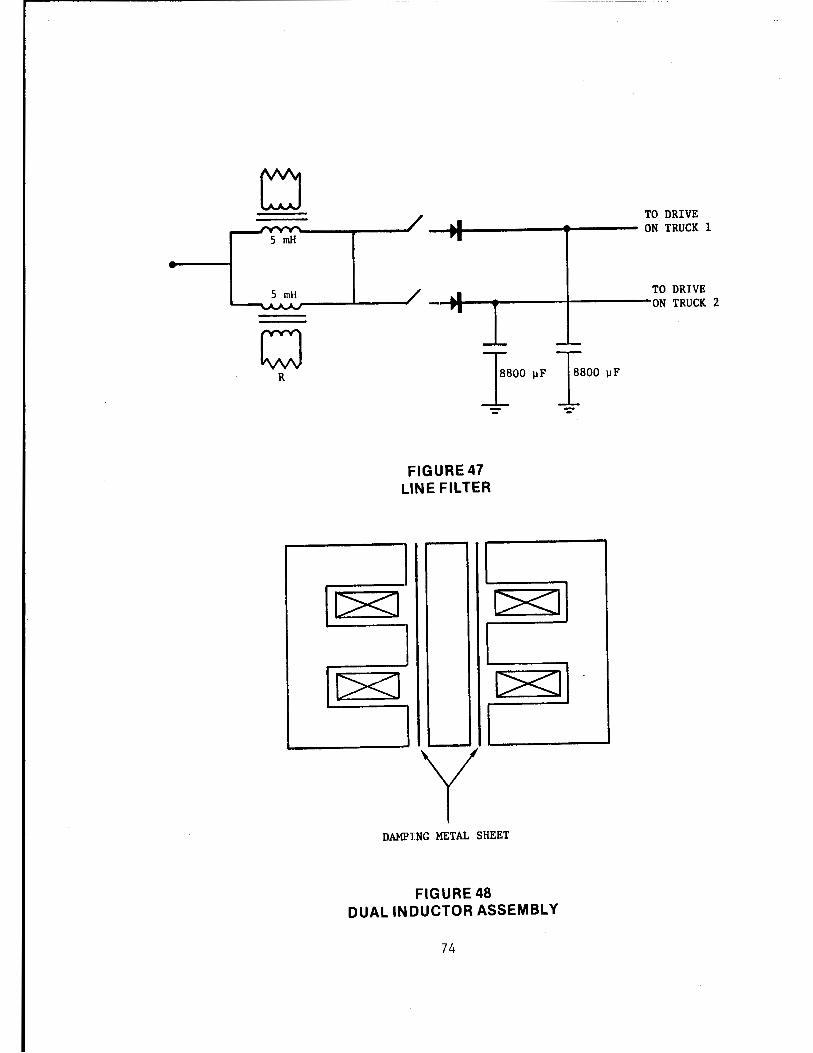
5 mH
Q R
C><I
C><l
TO DRIVE _,.._ ____ --4..,_ ___ ON TRUCK 1
TO DRIVE -ei1--------1-----0N TRUCK 2
I•• µF I•oo µF
FIGURE 47 LINE FILTER
y r><]
DAMPING METAL SHEET
FIGURE 48 DUAL INDUCTOR ASSEMBLY
74

-..J V,
500 Vdc
-- ·--- - ---· -- -· -- ---
X
-------------: } TO CYCLOCONVERTER
FIGURE 49 INVERTER CIRCUIT
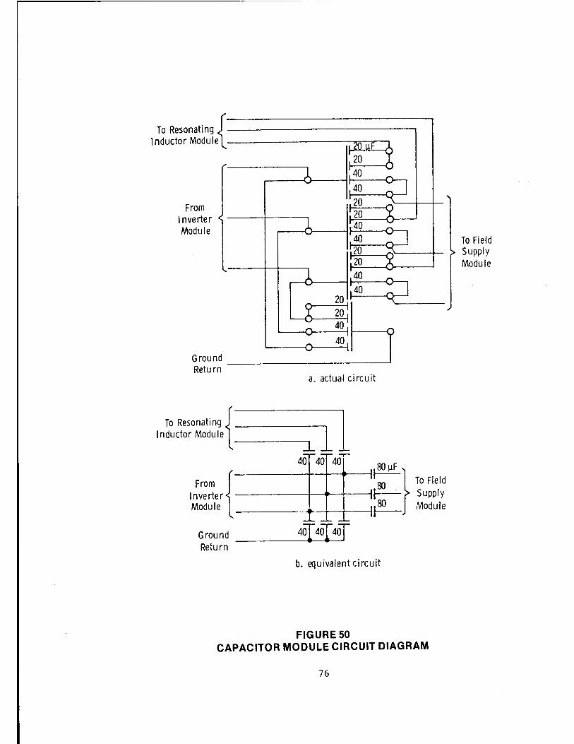
To Resonating (' _____________ ~ Inductor Madu leL
From Inverter Module
Ground Return--------------'
a. actual circuit
To Resonating { 1 Inductor Module 1
~l 40 40 40 80µF
Fro {-------~----.~} To Field lnve~er i-.:.:.-- Supply Module ~ Module
Ground _____ 4_of._4of_.._4_Jof Return
b. equivalent circuit
FIGURE 50 CAPACITOR MODULE CIRCUIT DIAGRAM
76
To Field Supply Module

• Traction Motor: The traction motor (one per truck) is a brushless four-pole machine with forced convection liquid cooling. In motoring it can produce a torque of 1560 lb-ft for a speed range of 0-1646 rpm and it can deliver a constant horsepower of 489 hp (365 kW) for a speed range of 1646-5642 rpm. It carries a rotating transformer-rotating rectifier on its shaft for supplying the field winding. A rotor position sensor is installed in one end of the motor. The rotor position sensor is installed in one end of the motor. The rotor is a one-piece forging with four poles. Laminated pole heads are bolted on the forging to hold the prewound field coils in place. The pole head also carries damper bars. To cool the motor a fire resistant silcone oil is sprayed on the stator conductors, the end turns of the rotor windings, and the rotating transformer/rectifier. The coolant is collected in a sump at the bottom of the motor frame and is recycled back to cooling assembly. Figure 52 shows a sectional view of the motor. It is about 48 inches long and weighs 1905 lbs.
Extensive computer simulations of the performance of this propulsion
system indicated that the system would in fact meet all the requirements.
5.4 Test Results
System level testing was performed using the total drive system . . (50 51)
During the system level testing ' , a large number of data points
were obtained at gradually increasing power level. These results are
illustrated in Figure 53. The torque-speed curves were also obtained
for various inverter frequencies during dynamometer testing. These
results are shown in Figure 54 where the torque discontinuity at a
speed of 2000 rmp is due to a change of control technique. Dynamic
braking performance was also obtained and compared with the predicted
performance as shown in Figure 55. Here the experimental data obtained
during component level testing and system level testing are compared
with analytical predictions.
During the extensive system level testing - February 1977 to
December 1977 - several unforeseen problems arose requiring extensive
circuit reconfigurations. Some of the problems involved the motor and
77

+C GROUP
+A GROUP -A GROUP
X X y __.,.Dlr-___._,..__•--i~- y
'---___ro,,,.o_~ z A X
z
-B GROUP
+B GROUP -C GROUP
ROTOR POSITION
SENSOR
X FIGURE 51
CYCLOCONVERTER POWER CIRCUIT
-------30.00-----, ROTARY J·,i..l·STATOR SALi ENT POLE
TRANSFORMER 'I' ROTOR
COOLANT RESERVOIR
FIGURE 52 AC TRACTION MOTOR
78
20.00 _.....,._DIA.

1600
1200
BOO
......... . 400 ..0
.-I I
.-I
.-I '--'
i:x:l ::::> CY P::: 0 H -400
-800
-1200
-1600
• ., •
• • MOTORING• •
• • • • • • • • • • •• • • •
• • • • ••
o 1q_oo 2000 0 0
~ 0 0
0
8 0
§0 & 0
0
0
0
490 hp
• • • •
• 3000 o 4000
0
8 0
0 0 0 0 0
0 0
BRAKING
0
• hp
5000 6000
• MOTORING
o BRAKING
REQUIREMENT
FIGURE 53 MOTORING/BRAKING TEST RESULTS
79
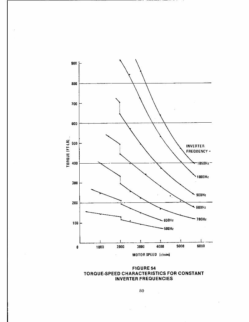
600
~ 500 ..:.. u..
w ::::, Q
~ 400 I-
300
200
100
0
~ INVERTER
1050Hz-
1000Hz
900Hz
800Hz
700Hz
1000 2000 3000 4000 5000 6000
MOTOR SPEED (r/mm)
FIGURE 54 TORQUE-SPEED CHARACTERISTICS FOR CONSTANT
INVERTER FREQUENCIES
80
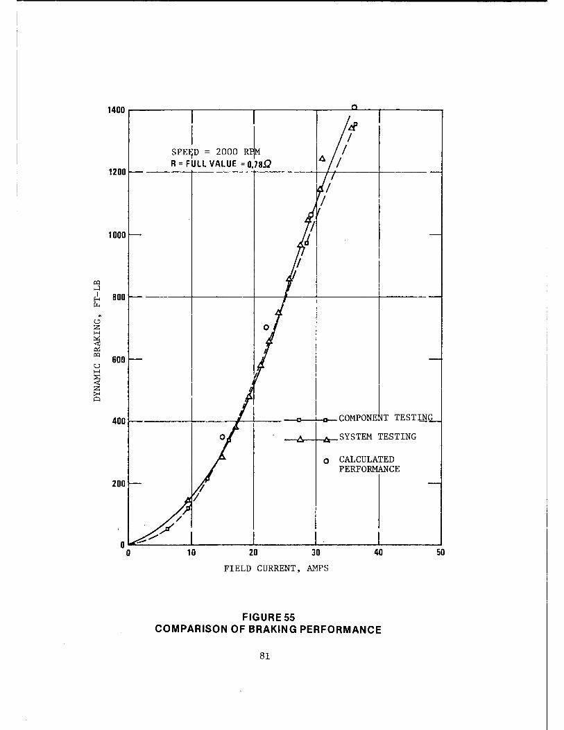
1400 ---------......------.------~--,----~
SPE~D = 2000 J 1200
R = FULL VALUE = 0,78.Q
1000
P'.l ...l
I 800 E-1 µ.,
~
c..!) z H
~ 0::: P'.l 600 u H
~ z >< Cl
400 ~ COMPONE T TESTIN
SYSTEM TESTING
0 CALCULATED PERFORMANCE
200
10 20 30 40 50
FIELD CURRENT, AMPS
FIGURE 55 COMPARISON OF BRAKING PERFORMANCE
81
and some involved power converters and control electronics. The
problems involving motor included Zener diode failures and other diode
failures in rotating solid state equipment used for field supply
and some minor problems with magnetic seals on bearings. The problems
with power and control electronics included insufficient or weak gate
drives, insufficient dv/dt and di/dt suppression, excessive noise in
control circuits and some generic problems due to interaction between
the inverter/cycloconverter and the motor. All of the above problem
areas were studied and most problems were resolved by end of 1977.
However, it was quite clear that substantial funding would be required
to complete the full-scale development program. The potential market
for such a propulsion system also appeared quite doubtful at the time.
This development of the Self-Synchronous Propulsion System was there
fore discontinued at the end of 1977.
The self-synchronous propulsion system used regenerative braking
to reduce energy consumption and a brushless synchronous motor to reduce
the high maintenance costs associated with de traction motors. The
system described in this section also used liquid cooling to obtain
high power densities. The resulting propulsion system required several
major new subsystems such as the inverter, the cycloconverter, the
rotating transformer, the rotating rectifier, the oil cooling system,
and complex electronic control systems. It is, therefore, doubtful
that this system would have improved reliability or reduced maintenance.
Hence, it does not appear to be a viable alternative to existing urban
rail transit propulsion systems.
This is, of course, not to say that synchronous machines cannot
be advantageously used for traction purposes. Other synchronous
machines, such as a permanent magnet, a homopolar machine or a
Lundell/Rice machine, might prove to be quite useful in spite of some
possible problem areas. With the permanent magnet machine, field
82

weakening is difficult and the motor needs to be de-energized
mechanically in case of a fault condition. The homopolar and Lundell/
Rice machines have a high commutating reactance. Also, any synchronous
machine would need an individual converter for control and may need
special starting circuits. But in spite of these difficulties, use
of synchronous motors would result in reduced inverter costs (inver
ters using natural-line or load - commutation are cheaper than those
using forced commutation) and hence, a synchronous motor should still
be considered as a viable alternative to a de traction motor.
5.5 A Locomotive Application
In the area of locomotive propulsion, the Russians are developing
a propulsion system using slip-ring type synchronous motors for their
VL-80 locomotive. As mentioned earlier, an induction motor system is
also being developed for this same VL-80 type locomotive. Because of
the broad gauge rail system, the Russian locomotive trucks can
accomodate synchronous motors, which are larger than equivalent induc
tion motors. Also, the Russian solid state technology is not as
advanced as that of the West and hence a possibility of reducing costs
of power converters by using a synchronous motor is more significant
in this context.
83

6.0 PROPULSION SYSTEM WITH ONBOARD ENERGY STORAGE
In the previous sections, the use of regenerative braking to
return at least part of the kinetic energy of the vehicle to the line
during braking was discussed. It was also pointed out that such
regeneration is possible if, and only if, the line is "receptive"
to this energy. The natural receptivity of a transit system depends
on several factors, such as the characteristics of substations, traffic
patterns, and the maximum allowable system voltage, all of which are
in a constant state of flux. The analysis of regeneration has to be
done essentially by obtaining the instantaneous energy balance on the
whole system. Thus the line is more receptive during peak hours when
one is more likely to find an accelerating train in the vicinity of a
decelerating train. Examples given previously show that, in general,
a typical transit system can be expected to regenerate 20-25 percent
of the propulsion energy on a long-term basis.
The problem of line receptivity can be eliminated if energy
storage capabilities can be provided on board the car, as shown in
Figure 56. The kinetic energy of the vehicle can now be temporarily
stored in the energy storage unit (ESU) during braking. This energy
can then be used to accelerate the vehicle when required. Some amount
of energy, however, is irretrievably lost in the process of effecting
these energy flows to and from the ESU. But since there is no need
to feed the vehicle kinetic energy back to the line, the resultant
energy consumption by the vehicle for a run does not depend on the
line receptivity.
In principle, any generic energy storage mechanism such as
batteries, compressed air, or a flywheel can be used for such a
system. In practice, however, the required storage capacity and the
charge/discharge rates are high enough to preclude the use of the
state-of-the-art batteries, and no major breakthroughs in battery
84

0:) V,
THIRD RAIL
PROPULSION SYSTEM
ENERGY FLOW
ENERGY FLOW DURING BRAKING
ENERGY STORAGE UNIT
DURING ACCELERATION
FIGURE 56 USEOFONBOARDENERGYSTORAGE
technology are expected to occur in the near future. A compressed
air system would be large and relatively inefficient. A flywheel
coupled to a de motor, on the other hand, is quite suitable for this
application.
6.1 R~32 Energy Storage Car for NYCTA
The first prototype equipment using onboard flywheel storage
was designed and built by Garrett and tested on two R-32 cars of NYCTA.
These cars are 60 feet long and weigh 35 tons without passengers.
These cars were modified with the following considerations:
• Only the hardware necessary to evaluate the effectiveness of the proposed propulsion system was replaced.
• Added equipment was packaged to conform to the NYCTA clearance envelope.
• Performance of the new propulsion system had to match that of the standard car in acceleration and braking, and
• The new system had to respond to the normal trainline commands.
The energy storage requirements were 3.2 kWh/car and the maximum
charging rate was 1.3 MW/car. This capability was obtained by having
two ESUs on each car. In practice a flywheel has to be able to store
about twice the energy that is to be transferred back and forth. If
a flywheel is operated over a speed range of 70-95 percent, about 40
percent of the maximum stored energy is transferable to and from the
flywheel unit. Hence the R-32 flywheel units were rated at 3.2 kWh
each at 100 percent speed and each car had two such flywheels. One
such unit is shown in Figure 57. The incremental weight of this
system was about 11,000 lbs.
Figure 58 shows the schematic of the total propulsion system. It
has four separately excited traction motors used in two parallel
groups, each having two motors in series. There are two ESUs, each
86

er: 0
~ z er: w .... -' <(
0 ::> 0 er: :I: (I)
z <( u.
-' w w :I: :i: > -' LL.
0)
.... Zen w .... :::iz - ::> C/)0 ~~
87
!::: z ::,
c., w z C,
<t ..... er: er: LI) 0 w ....
.... er: Cl)
z :::> >
w
~ C, ~ z
u. a: w
<( .... z z w
z N
<( 0
C")
a: 0 .... I
a: er: <( w c.,
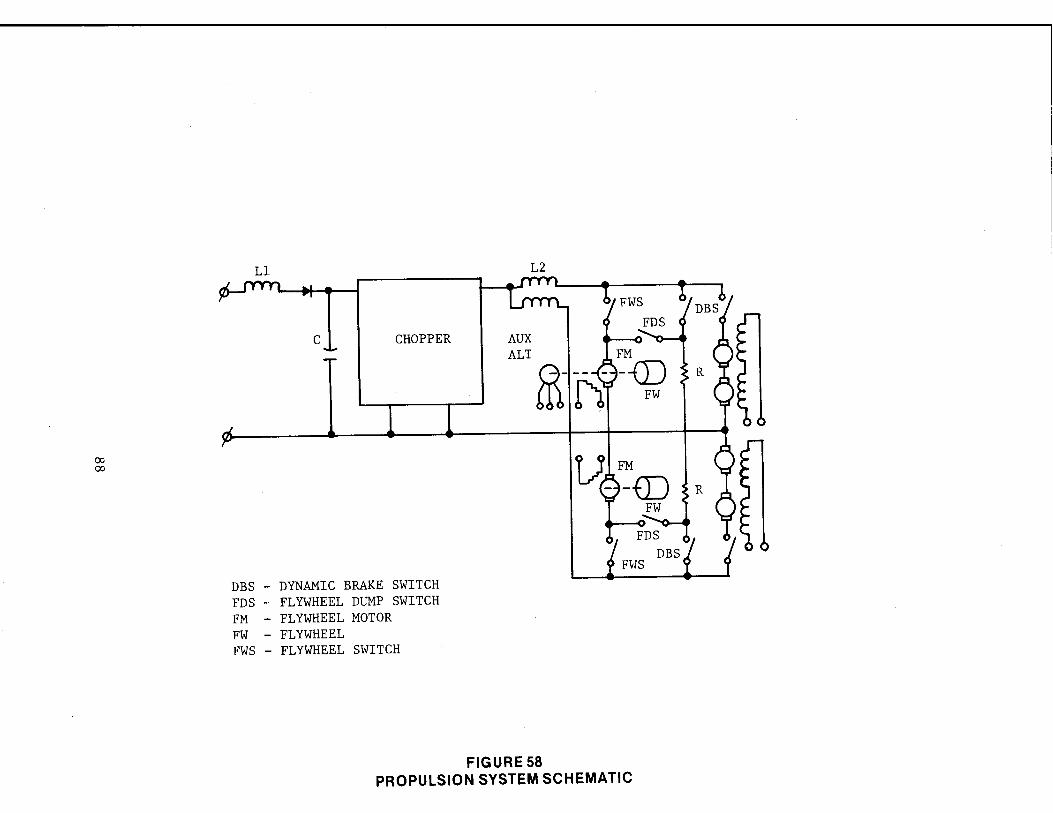
00 00
Ll
C CHOPPER
DBS - DYNAMIC BRAKE SWITCH FDS - FLYWHEEL DUMP SWITCH FM - FLYWHEEL MOTOR FW - FLYWHEEL FWS - FLYWHEEL SWITCH
L2
FIGURE 58 PROPULSION SYSTEM SCHEMATIC

consisting of a separately excited de motor driving a flywheel
through a gear train. An auxiliary alternator, mounted on one ESU,
is used to supply the auxiliary loads including the field windings
of the motor. The flywheel, made of four 2 inch thick steel discs,
rotates at a speed of 10,000-14,000 rpm under normal operation in an
evacuated (-0.5 psia) enclosure. The de motor, rated at 650 kW at
3000 rpm, drives the flywheel through a gear ratio of 3.3:1, thus
giving a maximum motor speed of 4250 rpm. The vacuum and lubricating
oil pumps are also driven by the motor/flywheel. The entire unit is
attached to the underframe of the car with rubber shock mounts.
The system operation can be described as follows. First, the
flywheels are started up by feeding the flywheel de motor armatures
through the chopper while the fields are supplied through onboard
batteries. The flywheels are charged up to an operating speed. At
about 40 percent speed (-5600 rpm) the alternator can supply all the
auxiliaries including the cooling fans. The system will remain
in this condition until vehicle acceleration is commanded.
When the vehicle is required to accelerate, the traction motors
are fully excited, the chopper is switched off and the traction motor
armatures are fed from the flywheel de machine working as a generator.
The current through traction motors is controlled by controlling the
field of the flywheel machine. This is identical to the classical
Ward-Leonard control of a de motor. The flywheel speed continues
to drop and when it drops below a certain speed, the chopper is
switched on again to maintain the required power. When the chopper
conduction ratio reaches unity, the traction motors and the flywheel
motor are controlled by field control.
89
Whenever a change in power is required it is obtained by taking
in power from the flywheel and/or the line as required, while always
maintaining the speed schedule for the flywheel.
The braking schedule of R-32 cars calls for a constan~ power
braking (0.32 MW/motor) between speeds 55-45 mph and a constant force
braking (~16,500 lbs. braking force for a vehicle of 112,000 lbs)
between speeds 45-9 mph, thus giving a deceleration of about 3 mphps.
At the start of braking, the flywheels are scheduled to be running at
about 10,000 rpm (~70 percent). During braking, the kinetic energy
of the vehicle is used to charge up the flywheel and they run at about
14,000 rpm (100 percent) at the end of the braking cycle, thus stating
1.6 kWh of•energy each. Braking of lighter cars, or braking from lower
speeds will cause less energy being stored in the flywheels. Sustained
braking of heavy cars on a downgrade, however, will warrant the use of
dynamic braking because the storage limit of the flywheel would other
wise be exceeded.
Whenever the vehicle is stopped, the flywheel continues to coast
down and if its speed drops below a certain speed, the chopper is
turned on to maintain its speed at the required level. The flywheels
can be shut down rapidly through a resistance grid when required,
such as at the end of the day.
A typical run between stations and the power flow are shown in
Figure 59. It can be seen that in addition to energy savings, the
peak power demanded from the line is reduced, resulting in improving
the line regulation as well as reducing demand charges for power
consumption.
Two converted R-32 cars were tested extensively at The Transportation
Test Center and on different lines of NYCTA(53
). These two cars were
90

t I+ II ~ .c
;:: .... "' ... QJ
;:: 0 a. C: 0
·,:;
1~ I
Acceleration Constant speed
Power from energy storage to traction motors
3rd rail power input
Power to overcome drag
Some 3rd rail power to energy storage if required
FIGURE 59
Energy pack charged
Brake
POWER FLOW DURING A TYPICAL RUN
91
Station stop
power returns to energy storage instead of generating heat

testing for about one year under non-revenue operation and then,
during a period of six months (February 1976 - August 1976), the cars
accumulated about a total of 26,000 revenue miles on different lines.
The energy savings demonstrated in comparison with the standard R-32
controlled cars are shown in Figure 60 for these lines.
In addition to the above testing, the energy consumption of
propulsion using cam control, propulsion using chopper control with
regenerative braking, and the above propulsion system was extensively
analyzed with the help of a computer simulation of the NYCTA "A"
line( 53). Various parameters such as track curves and grades, speed
restrictions, passenger loading and different duty cycles were con
sidered. The "A" line consists of 76 stops over a total round trip
of 47.23 miles at a schedule rate of 3 min/mile. The results of this
simulation showed an average energy savings of 30 percent (from ~5 kWh/
car-mile to ~3.5 kWh/car-mile) and a drop in the peak power demand of
as much as 50 percent. A typical energy flow for the car with an ESU'
is shown in Figure 61. The actual numbers are, of course, a function
of several variables and the numbers in the diagram are given for
purposes of comparison with similar computations given in Figures 9
and 28 for cam and chopper control.
6.2 ACT-1 Propulsion System
The next generation of an onboard ESU was developed under the
Advanced Concept Train (ACT-1) program of UMTA initiated in early
1972. This ESU was also developed by Garrett. Two cars with flywheel
propulsion were built and have been undergoing tests at the Transportation
Test Center since late 1977. Over a period of 15 months (October 1977 -
December 1977) the cars have run a total of 23,500 miles including
simulated revenue service for about 11,000 miles. The cars are about
75 feet long and weigh about 90,000 lbs when empty. The weight of
the propulsion equipment (excluding the traction motors) is about
92

'° w
D
MANHATTAN
N
THE BRONX
· TEST SCHEDULE
ENERGY LINE SAVINGS MILEAGE
A 32% 188
rt :jif •' ,,- ❖ ,~ X
QUEENS N 26% 92
E 31% 65
A El; 31% 82
AA 38% 79
B 28% 210
D 27% 155
F 28% 162
RJ 24% 87
RR 28% 35
FIGURE 60 ENERGY SAVINGS BY ON BOARD FLYWHEEL SYSTEM
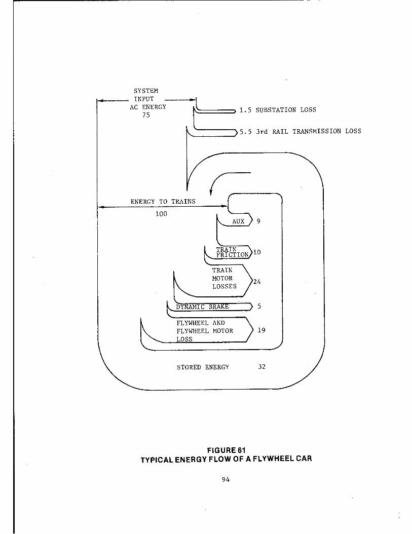
SYSTEM INPUT
AC ENERGY 75
5.5 3rd RAIL TRANSMISSION LOSS -------
c_ ENERGY TO TRAINS
100 AUX 9
TRAIN 10 FRICTION
TRAIN MOTOR 24 LOSSES
DYNAMIC BRAKE 5
FLYWHEEL AND FLYWHEEL MOTOR 19 LOSS
STORED ENERGY 32
FIGURE 61 TYPICAL ENERGY FLOW OF A FLYWHEEL CAR
94
14,000 lbs. This includes about 6,000 lbs for the ESU motor and about
5,500 lbs for the flywheel and the gearbox. Each flywheel, made of
0.1 inch thick steel laminations, is rated 4.5 kWh and there are two
such units in a car. Figures 62 and 63 show the ESU and the ACT-1
vehicle respectively.
Figure 64 shows the schematic of the propulsion system. There
are only two traction motors per car because the vehicle uses mono
motor trucks. It can be seen that the chopper used in the other design
has been eliminated. The flywheels are first started by drawing
power from the third rail and supplying the field winding from the
onboard batteries. The traction motors are started by supplying the
armature current from the flywheel motors acting like generators.
The flywheel acts as a prime mover and the field currents of the
flywheel-generators are controlled to supply the required currents
to the traction motors. The field windings of all the de machines
are supplied by an auxiliary alternator run by the flywheel itself.
The system behaves like the classical Ward-Leonard system and has
excellent control characteristics. The flywheel continues to decelerate
as the vehicle accelerates and after a certain speed, the third rail
supplies the cruising power to the motors. If under some operating
condition, the flywheel speed drops below a predetermined value, the
flywheel motors can be connected in series with the traction motors
so that the flywheel can be brought up to desired speed.
During the vehicle braking, the traction motors operate as genera
tors and drive the flywheel motors, thus storing the kinetic energy of
the vehicle into the flywheel. If the flywheel speed reaches the rated
maximum, the vehicle energy can be directed to a resistor bank for
dissipation.
95
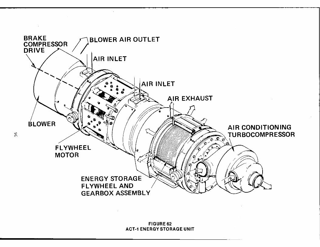
I.O C\
BRAKE COMPRESSOR DRIVE
\ ,/;BLOWER AIR OUTLET
- I I
AIR INLET
FLYWHEEL MOTOR
ENERGY STORAGE FLYWHEEL AND GEARBOX ASSEMBLY
FIGURE 62 ACT-1 ENERGY STORAGE UNIT
AIR CONDITIONING TURBOCOMPRESSOR

0
97
I.LI C") ..J (,0 (.)
I.LI ::I: a: I.LI ~> c,..-- I LL 1-
(.) <(

6.3 Improved Propulsion System for R-36 Cars of NYCTA
An improved version of the ACT-1 flywheel propulsion system
has been proposed by Garrett to NYCTA for a retrofit program on R-36
cars. This system, schematically shown in Figure 65, has only one
flywheel unit per car. The car has bimotor trucks and hence there are
four motors per car. The basic operation and the operating character
istics are similar to the ACT-1 system but the entire system has been
redesigned so as to reduce the overall complexity. Figure 66 shows
the new compact ESU unit for this system. A mulip-phase, 22-car
deployment program of such an R-36 retrofit is expected to begin in
the near future.
6.4 Noise and Vibrations
In spite of all the improvements to date, the noise and vibrations
are still the undesirable characteristics of the onboard ESU system.
The flywheel is rotating continuously and it is at peak speed in
stations when it is fully charged at the end of braking schedule.
In stations, therefore, a car with a flywheel is significantly noisy
when compared to a car without a flywheel. For a car in motion, however,
the increase in noise due to flywheel is insignificant. Similarly,
the energy storage unit causes additional vibrations in a car that
are especially noticeable in the vicinity of the storage unit. Although
the noise and vibrations could possibly be reduced further, it has to
be realized that this unit will alway increase the noise and vibration
levels in the car.
6.5 Additional Maintenance
The maintenance of de traction motors - repair and replacement
of brushgear, turning the commutators, rewinding of armatares, etc., -
is one of the major components of the overall maintenance costs of
transit cars. The required maintenance is so high that as many as
25 percent of traction motors are rewound every year on some transit
98
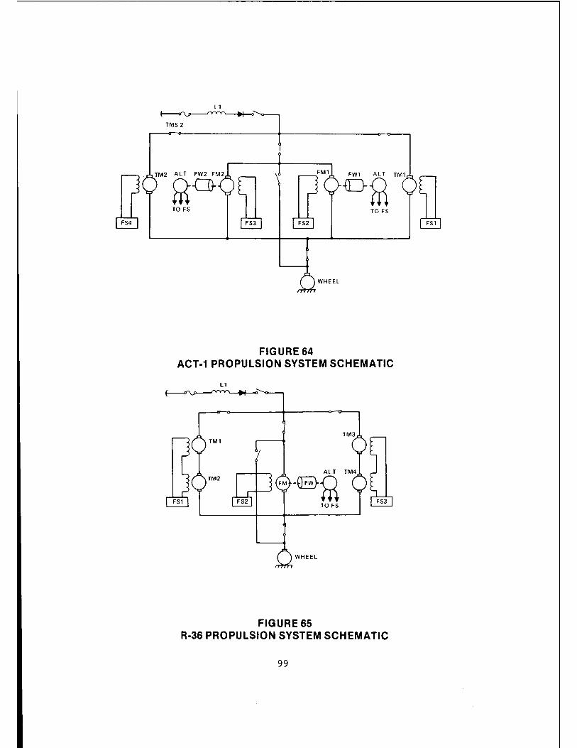
TM2 ALT FW2 FM2
20-TO FS TO FS
WHEEL
FIGURE 64 ACT-1 PROPULSION SYSTEM SCHEMATIC
TM1
ALT TM4 TM2 -~2
TO FS
WHEEL
FIGURE 65 R-36 PROPULSION SYSTEM SCHEMATIC
99

I-' 0 0
AIR OUTLET /)
BLOWER
BLOWER
MOTOR/GENERATOR
FLYWHEEL
AIR INLET
FIGURE 66 ESU FOR R-36
ALTERNATOR
/

properties. In view of this, the addition of another de motor to the
propulsion system should be considered as a significant disadvantage.
Moreover, other rotating equipment such as the flywheel, blower, and
gear box require maintenance. It is not clear how the total maintenance
costs of this system will compare with those of conventional cam and
chopper controlled equipment. Any definite conclusion in this regard
will have to wait until the necessary operating experience is obtained
on a sizable fleet of cars with such a system.
6.6 Gyroscopic Effects(55 )
The flywheel is a rotating mass and hence exhibits a gyroscopic
effect that must be considered while designing the energy storage
unit. The energy storage unit is mounted on the car with the spin
axis of the flywheel parallel to the longitudinal axis of the car.
Additional forces are, therefore, produced when a car negotiates a
curve or undergoes a pitch motion. For example, with the improved
propulsion system using one ESU, it has been estimated that for a 50 ft
car weighing about 100,000 lbs, an additional vertical force of about
684 lbs can be generated at each of the four ESU mounts when the car
goes through a curve of 145 ft radius at a speed of 33 mph. This
additional force is about 40 percent of the ESU weight at each mount.
Similary, if both ends of the car have a pitch motion of ±6 inches
at 1 cycle per second, the side loading on each mount is estimated to
increase by about 500 lbs. All these additional forces are quite
small compared to the total car weight and are not expected to have
any noticeable effect on the car performance or the operating life of
the components. However, when a single ESU is thus used, the effects
of these forces on car body motion must be evaluated.
101
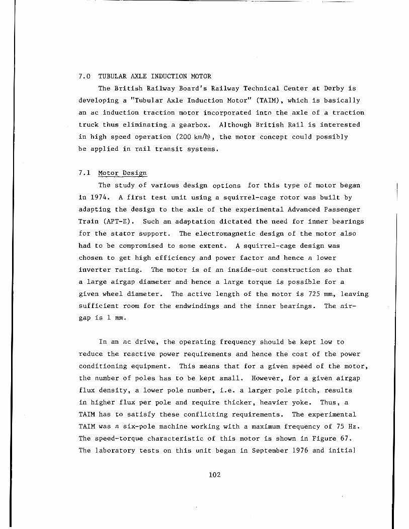
7.0 TUBULAR AXLE INDUCTION MOTOR
The British Railway Board's Railway Technical Center at Derby is
developing a "Tubular Axle Induction Motor" (TAIM), which is basically
an ac induction traction motor incorporated into the axle of a traction
truck thus eliminating a gearbox. Although British Rail is interested
in high speed operation (200 km/iv, the motor concept could possibly
be applied in rail transit systems.
7.1 Motor Design
The study of various design options for this type of motor began
in 1974. A first test unit using a squirrel-cage rotor was built by
adapting the design to the axle of the experimental Advanced Passenger
Train (APT-E). Such an adaptation dictated the need for inner bearings
for the stator support. The electromagnetic design of the motor also
had to be compromised to some extent. A squirrel-cage design was
chosen to get high efficiency and power factor and hence a lower
inverter rating. Lhe motor is of an inside-out construction so that
a large airgap diameter and hence a large torque is possible for a
given wheel diameter. The active length of the motor is 725 mm, leaving
sufficient room for the endwindings and the inner bearings. The air
gap is 1 mm.
In an ac drive, the operating frequency should be kept low to
reduce the reactive power requirements and hence the cost of the power
conditioning equipment. This means that for a given speed of the motor,
the number of poles has to be kept small. However, for a given airgap
flux density, a lower pole number, i.e. a larger pole pitch, results
in higher flux per pole and require thicker, heavier yoke. Thus, a
TAIM has to satisfy these conflicting requirements. The experimental
TAIM was a six-pole machine working with a maximum frequency of 75 Hz.
The speed-torque characteristic of this motor is shown in Figure 67.
The laboratory tests on this unit began in September 1976 and initial
102
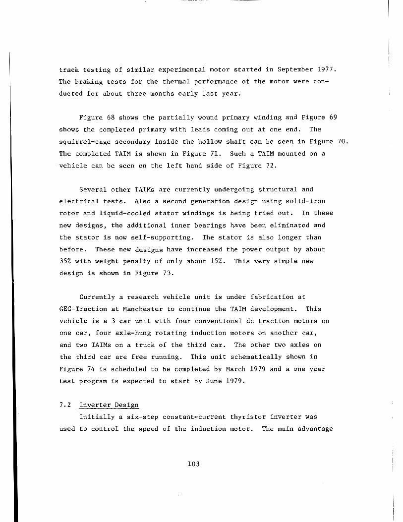
track testing of similar experimental motor started in September 1977.
The braking tests for the thermal performance of the motor were con
ducted for about three months early last year.
Figure 68 shows the partially wound primary winding and Figure 69
shows the completed primary with leads corning out at one end. The
squirrel-cage secondary inside the hollow shaft can be seen in Figure 70.
The completed TAIM is shown in Figure 71. Such a TAIM mounted on a
vehicle can be seen on the left hand side of Figure 72.
Several other TAIMs are currently undergoing structural and
electrical tests. Also a second generation design using solid-iron
rotor and liquid-cooled stator windings is being tried out. In these
new designs, the additional inner bearings have been eliminated and
the stator is now self-supporting. The stator is also longer than
before. These new designs have increased the power output by about
35% with weight penalty of only about 15%. This very simple new
design is shown in Figure 73.
Currently a research vehicle unit is under fabrication at
GEC-Traction at Manchester to continue the TAIM development. This
vehicle is a 3-car unit with four conventional de traction motors on
one car, four axle-hung rotating induction motors on another car,
and two TAIMs on a truck of the third car. The other two axles on
the third car are free running. This unit schematically shown in
Figure 74 is scheduled to be completed by March 1979 and a one year
test program is expected to start by June 1979.
7.2 Inverter Design
Initially a six-step constant-current thyristor inverter was
used to control the speed of the induction motor. The main advantage
103
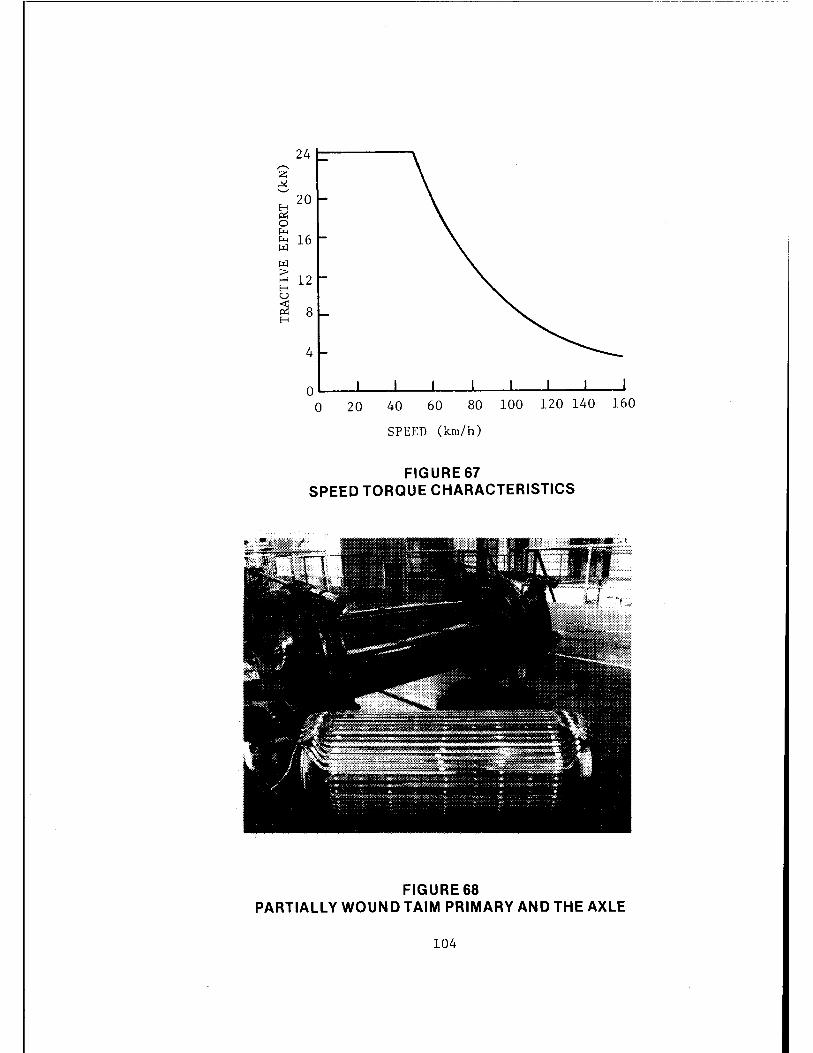
,,...._ z ~ ,._., H 20 ~ 0 ~ ~ 16 ~
~
~ 12 H u ~ 8 H
4
0 L--L-----lL-----L-----L----L-.....L---'--~
0 20 40 60 80 100 120 140 160
SPEED (km/h)
FIGURE 67 SPEED TORQUE CHARACTERISTICS
FIGURE 68 PARTIALLY WOUND TAIM PRIMARY AND THE AXLE
104
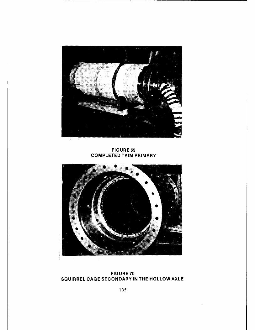
FIGURE 69 COMPLETED TAIM PRIMARY
FIGURE 70 SQUIRREL CAGE SECONDARY IN THE HOLLOW AXLE
105

FIGURE 71 COMPLETELY ASSEMBLED TAIM
FIGURE 72 TAIM MOUNTED ON A VEHICLE
106

of this type of inverter is its low cost and simplicity, but it is
not very suitable for systems requiring extensive low speed operation.
Such an operation results in unacceptably high torque pulsations and
high motor losses. PWM inverters can be used to alleviate this problem,
but thyristor PWM inverters are quite expensive. British Rail firmly
believes that with the on-going development of power transistors, PWM
inverters using power transistors will be the induction motor controllers
of the future. A 50 kVA PWM transistor inverter is presently operating
at Derby and a full power inverter for supplying the TAIM is currently
under development.
The tubular axle induction motor is a very interesting concept
but its development will take several more years. Its suitability
for propulsion of urban rail vehicles, therefore, cannot be evaluated
at this time.
107

AIR INLET
00 00 A i i t I
Axle Hung Rotating Induction Motors
CABLE DUCT
I-SECTION AXLE BEAM
FIGURE 73 NEW TAIM DESIGN
00 00 y y Free TA!Ms
Running
FIGURE 74
WHEEL BEARINGS
STATOR LAMINATIONS
00 00 t t
I t t
Conventional DC Motors
BRITISH RAIL RESEARCH VEHICLE
108

8.0 CONCLUSIONS
From this review of the state-of-the-art and on-going development
of electric traction systems it is possible to draw the following
conclusions:
AC Propulsion Using Induction Motors
AC propulsion systems using induction motors supplied by PWM
inverters have completed prototype testing and are now in revenue ser
vice. Several locomotives are now in regular operation on the German
and Swiss railway networks. Subway cars using ac drives are in revenue
service in Berlin and Vienna, and they are undergoing pre-service testing
in Helsinki.
At present, ac drives using induction motors are more expen
sive that the de chopper systems for urban transit - by 0-20% depending
on system characteristics such as line receptivity for braking energy,
allowable wheel diameter variations and auxiliary power system design.
It is expected, however, that with falling prices of solid state equip
ment as well as savings in traction motor maintenance, these ac drives
can be offered at very competitive prices within the next 3-5 years. The
future of ac drives will depend very much on the operating experience
obtained by different transit properties running the prototype vehicles.
There is no doubt that the equipment meets all the technical requirements
but there is still some uncertainty about the failure rate and mainte
nance costs associated with the PWM or other type of inverter. If the
prototype equipment performs as well as expected, the ac drives will
become standard equipment beyond a period of about five years, at least
in Germany. If ac drives are introduced in the U.S. in any appreciable
numbers, it would probably be done in the late 1980's at the earliest.
DC Propulsion with Cam Control
DC drives with cam control (rheostatic control) are the
classical traction systems for urban rail transit vehicles. The torque-
109

speed characteristic of the motor is well suited for transit applica
tions and the speed of the motor is easily controlled. The cam con
troller is well proven technology and fairly simple. Alternative
propulsion systems may be more advantageous in areas of maintenance
costs, energy consumption (efficiency and regeneration) and smoothness
of control.
The transit properties that have a big investment in conventional
cam controlled equipment may consider that the efficiency resulting
from limiting the number of types of equipment to be maintained out
weigh the advantages of alternative propulsion systems. The NYCTA
(New York) and CTA (Chicago) together operate more than 80 percent of
the U.S. fleet of cars and thus represent a major share of this market.
Both these properties are actively evaluating alternate propulsion
systems. However, CTA has decided to buy rheostatic control equipment
for its current order and if NYCTA buys any cars in the near future
it will most probably opt for rheostatic control as well.
DC Propulsion with Chopper Control
Chopper control is a significant improvement over the conven
tional cam control, particularly in providing regenerative braking. The
first prototype de chopper systems were tested during the late 1960's,
and they have now evolved into a proven reliable control technology.
Street and subway cars with chopper control are in regular operation on
transit lines in several European and North American cities.
It is likely that the de chopper will be the system of choice
for the next five years. The cost of energy has now increased to
the point where the initial incremental cost for chopper control can
generally be justified on a life-cycle cost basis. The future of
chopper systems, however, is clearly linked with the pace of continued
development and acceptance of ac drive systems using induction motors.
Some transit properties, especially in Germany, believe that sufficient
110
data about the technical performance and the operating experience of
ac drives will be available in the next 3-5 years. Therefore, they
expect to continue to use cam controllers for a few more years and
then introduce new drives.
AC Propulsion Using Synchronous Motors
The cost of solid state power conversion can be significantly
reduced with the use of synchronous motors. This is because inexpensive
line commutated inverters can be used by operating the synchronous motors
at leading power factor. AC drives using synchronous motors, however,
are not currently under active development anywhere and a major program
of development of such a drive in the U.S. was discontinued over a year
ago.
Since ac drives using synchronous motors are not currently
under active development, it is unlikely that they would be considered
competitive for a period of fifteen years or so. Drives using permanent
magnet or other types of synchronous motors will, no doubt, be con
tinually evaluated for possible development.
On-Board Energy Storage.
A propulsion system using onboard energy storage has some very
significant features such as regeneration even without any line recep
tivity and electronic control at lower power levels.
Onboard energy storage has the potential for improving traction
system efficiency. Higher weight, increased noise and vibrations and
possibly increased maintenance are some of the disadvantages of
the system. The system, therefore, opens a number of important
111
"retrofit" options for application on the existing properties with
old wayside equipment. Any final judgement on such possibilities
will, of course, have to come after some operating experience is
obtained on a sizable fleet of such cars.
Tubular Axle Induction Motor
The tubular axle induction motor is a very interesting and
attractive concept for high speed transportation although its suit
ability for low speed urban vehicles has not been investigated in
detail. Any judgement on the tubular axle induction motor concept
can be made only after evaluating the results of operational testing
and hence will have to wait for several more years.
112

LIST OF REFERENCES
1. "Electrical Equipment for Subway Cars with Rheostatic and Chopper Control," Pamphlet TB40-101E Edition 1 of Transport Division, ASEA, Sweden.
2. Gardner, A.L., "Propulsion and Automation Equipment for PATCO's Rapid Transit Cars," Trans. IEEE., Vol. IGA-7, No. 6, pp. 760-768, (1971).
3. "The Freiburg Eight-Axle Articulated Street Car - Electrical Equipment," Brochure Vl/498E 05 73 of AEG-Telefunken, West Berlin.
4. "U-Bahn-Wagen Serie F76," Brochure N3/594/1177 of AEG Telefunken, West Berlin (in German).
5. "Optimization of Power Resources," Report No. IT-09-0023-TSC210 by Gibbs and Hill, Inc., New York.
6. "Energy Conservation in the New York Subway System," Report by School of Engineering and Applied Science of Columbia University, New York (1976).
7. Wagner, R., "Thyristor Chopper Controls for DC Traction Systems," Siemens Review, Vol. XLII, No. 1, pp. 39-43, (1975).
8. Wajima, K., et.al., "High-Speed Thyristors and Their Applications," Hitachi Review, Vol. 24, No. 6, pp~ 259-67, (1975).
9. Tsuboi, T., et. al., "Newly Developed Thyristor Chopper Equipment for Electric Railcars," Trans. IEEE, Vol. IA-9, No. 3, pp. 294-301, (1973).
10. Kimura, K., et. al., "Chopper Control System for Electric Cars," Hitachi Review, Vol. 27, No. 2, pp. 77-84, (1978).
11. Sawa, K., et. al., "Thyristor Chopper Controller for Type 270 Electric Car," Fuji Electric Review, Vol. 19, No. 2. (1973).
12. Voss, U., "Electronic Controls for Rapid Transit," Brochure N3/578E 04 77 of AEG Telefunken, West Berlin.
13. Voss, U., "Chopper Technology for Rapid Transit," Brochure N3/589E/ll 77 of AEG Telefunken, West Berlin.
14. Ashiya, M., et. al., "3000 V Chopper-Controlled Rail Cars for Spain's Renfe," Mitsubishi Electric Engineer, No. 3, pp. 1-6, (1977).
113
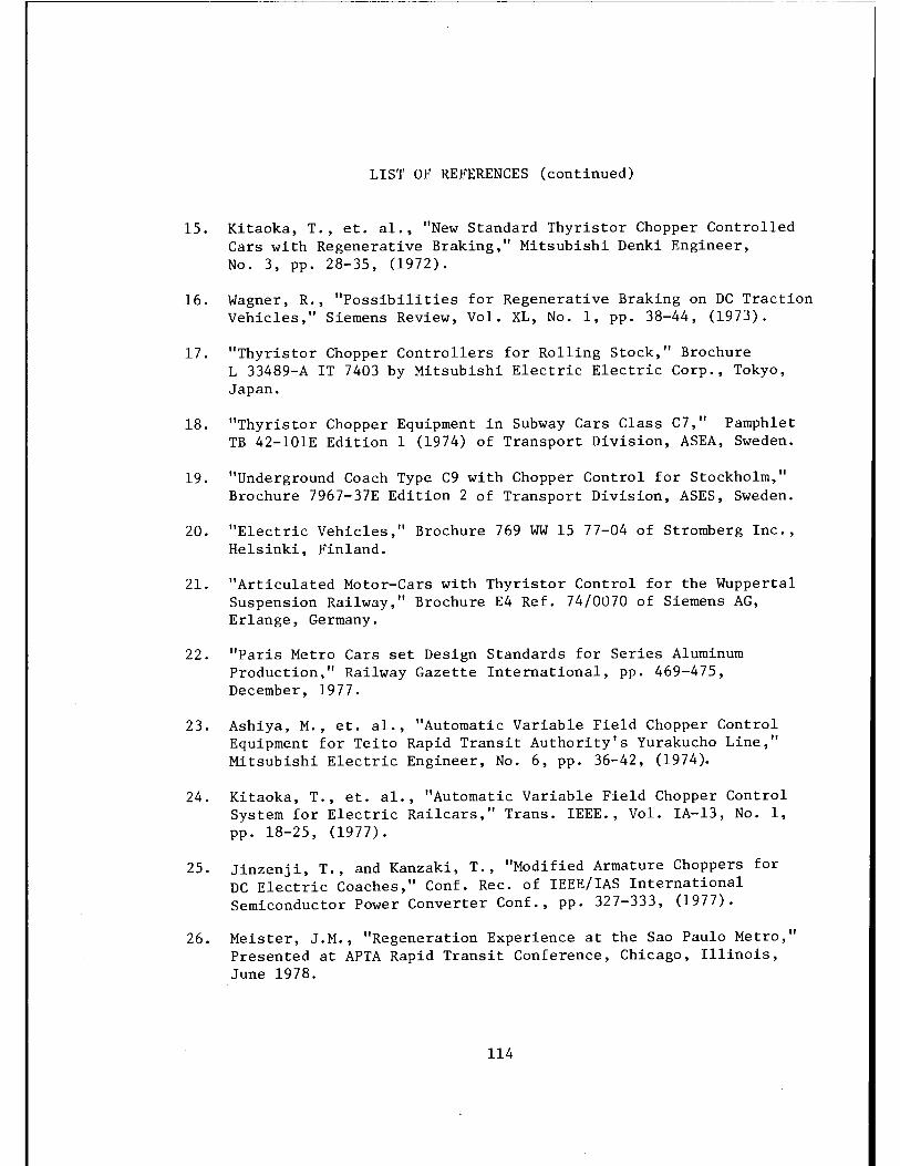
LIST OF REFERENCES (continued)
15. Kitaoka, T., et. al., "New Standard Thyristor Chopper Controlled Cars with Regenerative Braking," Mitsubishi Denki Engineer, No. 3, pp. 28-35, (1972).
16. Wagner, R., "Possibilities for Regenerative Braking on DC Traction Vehicles," Siemens Review, Vol. XL, No. 1, pp. 38-44, (1973).
17. "Thyristor Chopper Controllers for Rolling Stock," Brochure L 33489-A IT 7403 by Mitsubishi Electric Electric Corp., Tokyo, Japan.
18. "Thyristor Chopper Equipment in Subway Cars Class C7," Pamphlet TB 42-lOlE Edition 1 (1974) of Transport Division, ASEA, Sweden.
19. "Underground Coach Type C9 with Chopper Control for Stockholm," Brochure 7967-37E Edition 2 of Transport Division, ASES, Sweden.
20. "Electric Vehicles," Brochure 769 WW 15 77-04 of Stromberg Inc., Helsinki, Finland.
21. "Articulated Motor-Cars with Thyristor Control for the Wuppertal Suspension Railway," Brochure E4 Ref. 74/0070 of Siemens AG, Erlange, Germany.
22. "Paris Metro Cars set Design Standards for Series Aluminum Production," Railway Gazette International, pp. 469-475, December, 1977.
23. Ashiya, M., et. al., "Automatic Variable Field Chopper Control Equipment for Teito Rapid Transit Authority's Yurakucho Line," Mitsubishi Electric Engineer, No. 6, pp. 36-42, (1974).
24. Kitaoka, T., et. al., "Automatic Variable Field Chopper Control System for Electric Railcars," Trans. IEEE., Vol. IA-13, No. 1, pp. 18-25, (1977).
25. Jinzenji, T., and Kanzaki, T., "Modified Armature Choppers for DC Electric Coaches," Conf. Rec. of IEEE/IAS International Semiconductor Power Converter Conf., pp. 327-333, (1977).
26. Meister, J.M., "Regeneration Experience at the Sao Paulo Metro," Presented at APTA Rapid Transit Conference, Chicago, Illinois, June 1978.
114
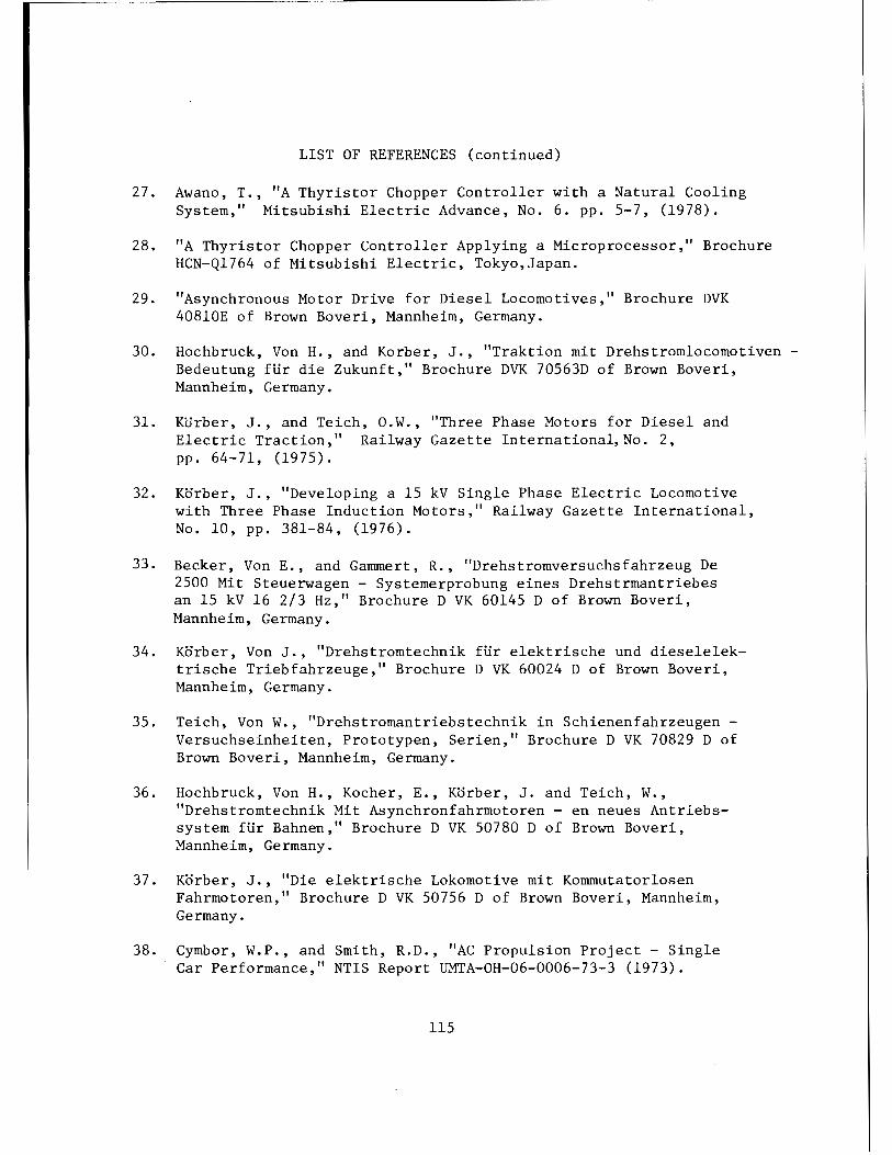
LIST OF REFERENCES (continued)
27. Awano, T., "A Thyristor Chopper Controller with a Natural Cooling System," Mitsubishi Electric Advance, No. 6. pp. 5-7, (1978).
28. "A Thyristor Chopper Controller Applying a Microprocessor," Brochure HCN-Ql764 of Mitsubishi Electric, Tokyo,Japan.
29. "Asynchronous Motor Drive for Diesel Locomotives," Brochure DVK 40810E of Brown Boveri, Mannheim, Germany.
30. Hochbruck, Von H., and Korber, J., "Traktion mit Drehstromlocomotiven -Bedeutung ftir die Zukunft," Brochure DVK 70563D of Brown Boveri, Mannheim, Germany.
31. KlJrber, J., and Teich, O.W., "Three Phase Motors for Diesel and Electric Traction,'' Railway Gazette International,No. 2, pp. 64-71, (1975).
32. Korber, J., "Developing a 15 kV Single Phase Electric Locomotive with Three Phase Induction Motors," Railway Gazette International, No. 10, pp. 381-84, (1976).
33. Becker, Von E., and Gammert, R., "Drehstromversuchsfahrzeug De 2500 Mit Steuerwagen - Systemerprobung eines Drehstrmantriebes an 15 kV 16 2/3 Hz," Brochure D VK 60145 D of Brown Boveri, Mannheim, Germany.
34. Korber, Von J., "Drehstromtechnik ftir elektrische und dieselelektrische Triebfahrzeuge," Brochure D VK 60024 D of Brown Boveri, Mannheim, Germany.
35. Teich, Von W., "Drehstromantriebstechnik in Schienenfahrzeugen -Versuchseinheiten, Prototypen, Serien," Brochure D VK 70829 D of Brown Boveri, Mannheim, Germany.
36. Hochbruck, Von H., Kocher, E., Korber, J. and Teich, W., "Drehstromtechnik Mit Asynchronfahrmotoren - en neues Antriebssystem ftir Bahnen," Brochure D VK 50780 D of Brown Boveri, Mannheim, Germany.
37. Korber, J., "Die elektrische Lokomotive mit Kommutatorlosen Fahrmotoren," Brochure D VK 50756 D of Brown Boveri, Mannheim, Germany.
38. Cymbor, W.P., and Smith, R.D., "AC Propulsion Project - Single Car Performance," NTIS Report UMTA-OH-06-0006-73-3 (1973).
115
LIST OF REFERENCES (continued)
39. "Inverter Controlled AC Induction Motor Drives in Vehicles," Brochure 772 WW125 75-03 of Stromberg Inc., Helsinki, Finland.
40. Ciessow, G., Golz, G., and Grumbrecht, P., "Three Phase AC Drive Systems for Traction Vehicles," AEG Telefunken Progress, Vol. 3, pp. 88-96 (1977).
41. "Drive Equipment with Three Phase Traction Motors for the Berlin Subway," Brochure N3/575E 05 77 of AEG-Telefunken, West Berlin.
42. Golz, G., et. al., "Wirkungsweise Neuartiger Pulsstromrichter," Elektrotechnische Zeitschrift, Vol. 98, No. 5, pp. 346-49, (1977).
43. Kratz, G., "Der Drehstrom-Asynchronmotor als neuer Fahrmotor fUr die Berliner U-Bahn," Der Stadtverkehr Vol. 22, No. 2, pp. 83-87, (1977).
44. Rudiger, W., and Brunnecker, U., "Siemens Tests AC Motors on a Tramcar," Railway Gazette International,No. 6, pp. 228-229, (1976).
45. Meissen, W., and Sauer, H., "Drehstromantrieb fUr Schienefahrzeuge am Gleich - und Wechselstrom -Fahrdraht," Eisenbahntechnische Rundschau Vol. 26, No. 7/8, pp. 445-52, (1977).
46. "DC Operated Double Unit with AC Three Phase Drives and Regenerative Brake of the Vienne Underground," Brochure El, E4 78/3 of Siemens, Erlangen, Germany.
47. Plunkett, A.B., and Plette, D.L., "Inverter-Induction Motor Drive for Transit Cars." Trans. IEEE. Vol. IA-13, No. 1, pp. 26-37, (1977).
48. Mitsuhashi, E., et. al., "Induction Motor Drive by High Frequency Pulse Width Modulation Inverter," Brochure HCN-Ql763 of Mitsubishi Electric, Tokyo, Japan.
49. Bourbeau, F.J., "Synchronous Motor Railcar Propulsion," Trans. IEEE,Vol. IA-13, No. 1, pp. 8-17, (1977).
50. "Self-Synchronous Propulsion System for Rapid Transit Railcars," Final Project Report, Vol. I, Report R78-14 by Delco Electronics, Santa Barbara, California (1978).
51. "Self Synchronous Propulsion System for Rapid Transit Railcars," Final Project Report, Vol. II, Report R78-14 by Delco Electronics, Santa Barbara, California (1978).
116

LIST OF REFERENCES (concluded)
52. Bourbeau, F.J., "Wide Speed Range Cycloconverter - AC Motor Drives Operating from Utility Frequency Power," Con£. Rec. of IEEE/IAS International Semiconductor Power Converter Conf., pp. 320-326, (1977).
53. Weinstein, C.H., "R-32 Energy Storage Propulsion System," Presented at IEEE Con£. on the Energy Crisis and Rail Transportation, New York, February 1976.
54. "Urban Rapid Rail Vehicle and Systems Program," NTIS Report No. UMTA-IT-06-0026-78-1, (1977).
55. "Energy Storage Propulsion System for New York City Transit Car," Report 77-14203-2 Addendum 3 of Garrett AiResearch Manufacturing Co., California (1977).
117

APPENDIX I
DIFFERENT TYPES OF TRACTION MOTORS
1.0 DC MOTOR
The essential components of a de machine are shown in Figure 75
and the machine is schematically represented in Figure 76. As can be
seen, the stator has salient poles excited by one or more field coils.
The airgap flux distribution created by the field excitation is cen
tered on the axis of the field pole, as shown in Figure 77. The arm
ature of a de machine is a winding that carries current through the
brushes and the connnutator. The current through an armature coil
reverses as that coil goes under the brush, as shown in Figure 78.
This current reversal is called commutation. The airgap flux distri
bution created by the armature current is centered on the brush-axis.
Under normal operating conditions, the brushes are located on the inter
polar axis - i.e., an axis displaced by 90 electrical degrees from
the field axis. The armature reaction flux increases the flux under
one pole-tip while decreasing the flux under the other pole-tip (also
shown in Figure 77). For linear magnetic materials, therefore, the
flux per pole is not affected by armature reaction. With saturation
of the iron, however, there is a net resultant reduction of the flux
per pole. In addition to this demagnetizing effect, the armature
reaction also has an adverse effect on connnutation. As shown in
Figure 78, a coil undergoing commutation is in transition between two
groups of armature coils. The current at the end'of the commutation
period must be equal and opposite to that at the beginning. For a short
time during connnutation, the armature coil is, in fact, short circuited
by the brush. It can be said that generally the resultant voltage
induced in this coil from different sources should be zero in order to
achieve linear commutation of current through the coil. This is usually
achieved by introducing an appropriate flux density in the interpolar
region by means of small narrow poles located between the main poles.
119
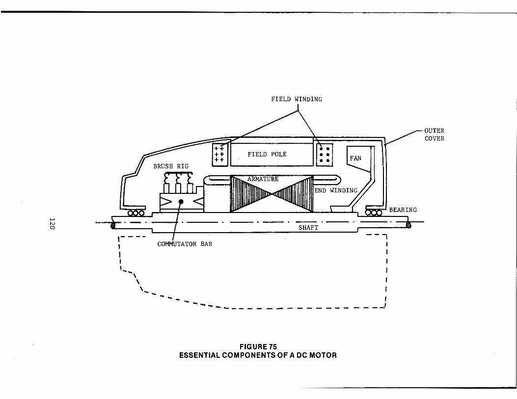
..... N 0
FIELD WINDING
FIELD POLE
BRUSH RIG
---•·-. - . ,- - - -1 I I ,_ -,
\ ,_ -
SHAFT
COMMUTATOR BAR
--- ----- ----------------
FIGURE 75 ESSENTIAL COMPONENTS OF A DC MOTOR
FAN
XX>< 1 BEARING
--7 I I
I - - _ _J
OUTER COVER

FINELY DISTRIBUTED e CONDUCTORS ON
ARMATURE
FLUX-DENSITY DISTRIBUTION ARMATURE ALONE
FIELD WINDING
MAIN FIELD POLES
BRUSHES
FIGURE 76 DC MOTOR SCHEMATIC
~ I ~
I I I
I
I
I GENERATOR I ROTATION I MOTOR ROTATION
•\ I \ ~
I FLUX-DENSITY .....--1" ·,,_ - ,_...;.;;;~ I DISTRIBUTION ·i
MAIN FIELD ALONE
FIGURE 77
t V
J
FIELD COIL
RESULTANT FLUX-DENSITY DISTRIBUTION
AIRGAP FLUX DISTRIBUTION IN A DC MACHINE
121

f-' N N
½I -a
1 2
+ -- -- kl 2 a
4 5
1
-
I a
3 4
FIGURE 78
½I a
5
- -
-
CURRENT REVERSAL DURING COMMUTATION
0 -- --½I a
-

These auxiliary poles are called interpoles. The polarity of an
interpole in a de motor is that of the main pole just behind it.
For motors subjected to heavy overloads or rapidly changing
loads or for motors operating under a weak field condition, the armature
reaction is compensated by using paleface windings. These windings
carry currents in a direction opposite to that of armature winding
facing them. Such a winding is called a compensating winding.
Figure 79 shows a de machine having interpoles and compensating windings.
Figure 80 shows the field structure and different windings in a de
motor. Figures 81 and 82 show the armature, the commutator and the
brushgear.
In general, there are several ways to excite one or more field
windings as shown in Figure 83. However, series excitation of the
field winding is the most common method for traction application.
1.1 Operating Characteristics
The operating characteristics of a de motor can be explained with
the help of the following relationships:
where
V = E + I r a a
E = K ~N e
V - terminal voltage
E - armature back emf
I - armature current a
r - armature resistance plus additional (series field or external) a
resistance, if any
123

I-' N .i:,-
• X
• X
~~- ......
LCOMPENSATING WINDING
"-COMMUTATOR
X
X
MAIN POLE
• X
• X
ROTATION
IC• c•' I "-- BRUSHES
FIGURE 79
~ INTERPOLE
• • X •
• • X •
DC MOTOR WITH INTERPOLES AND COMPENSATING WINDINGS
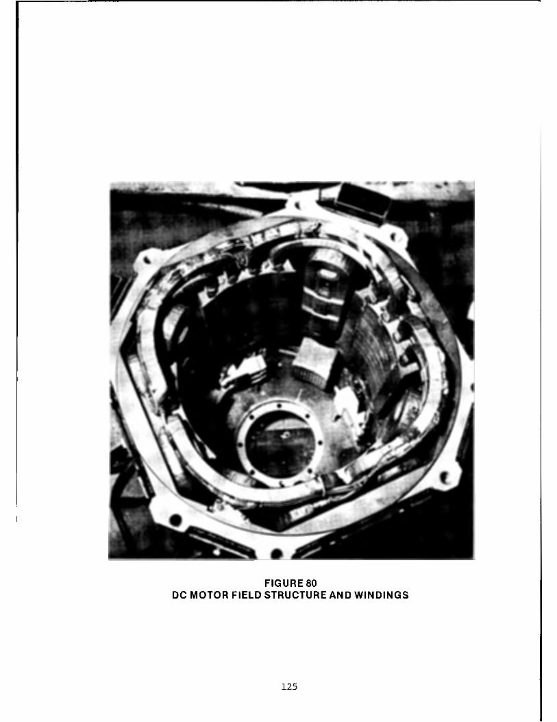
FIGURE 80 DC MOTOR FIELD STRUCTURE AND WINDINGS
125
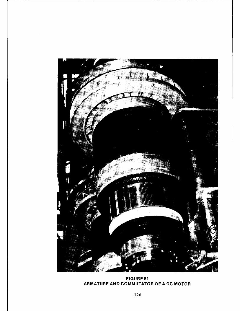
FIGURE 81 ARMATURE AND COMMUTATOR OF A DC MOTOR
126
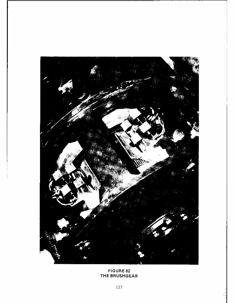
FIGURE 82 THE BRUSHGEAR
127

Series Shunt
Short-shunt Compound Long-shunt Compound
Separate
FIGURE83 METHODS OF FIELD EXCITATION
128

cp - flux per pole
N - speed
T - electromagnetic torque
K e' K t - constants
From these relationships one can obtain the speed of the motor as
V - I r N = ___ a_a_
Ke• cp
Under steady state conditions, the motor operates at a speed
where the electromagnetic torque generated by the motor equals the
load torque. The speed of operation, therefore, can be controlled
by controlling the armature (I) or the field(~). Also, the back a
emf Eis zero at start and hence the armature current I has to be a
limited either by reducing the voltage or by connecting external
resistances in series with the armature and then cutting them out,
manually or automatically, as the motor comes up to speed. Such a
starting process is shown in Figure 84.
1.2 Speed Control of DC Motors
DC motors in general are very much adaptable to adjustable-speed
application. In fact, easy control of the speed by several methods
is one of the important reasons for their wide application in propul
sion and in other industrial drives. The armature control and the
field control are the two basic methods of speed control. The
characteristics of these two control methods,shown in Figure 85,are
as follows.
1.2.1 Armature Control
As the name suggests, this method involves a control of the arma
ture circuit - reducing the armature voltage or inserting external
resistances in the armature circuit. If more than one motor is to be
129
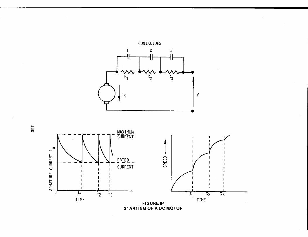
I--' w 0
Rl
! 1.
MAXIMUM - MRtNT
res ......
RATED 1-z LJ.J c:::: c::: ::::> u :- CURRENT LJ.J c::: ::::> l-ex: :E c::: CX: I • •
0 t, t2 t3 TIME
CONTACTORS 2 3
R2 R3
t 0 LJ.J LJ.J c.. (/)
FIGURE 84 STARTING OF A DC MOTOR
V
t, -c2 3 TIME
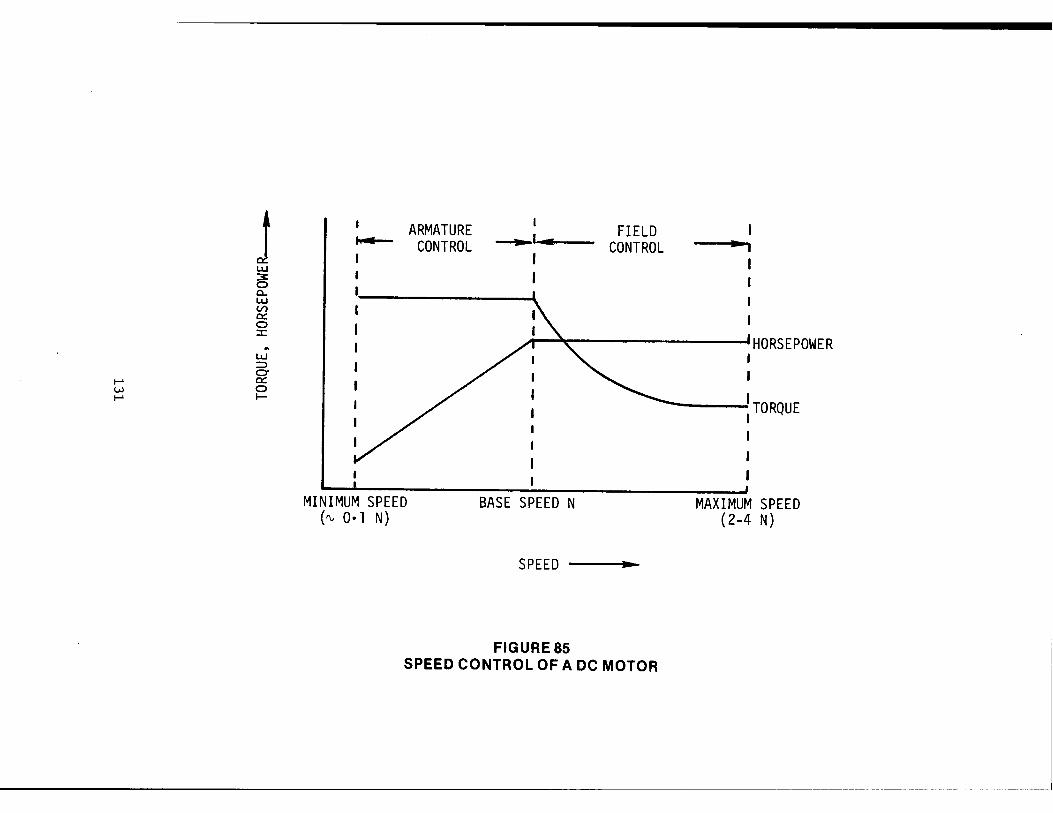
...... w ......
J LJ.J
~ 0.. LJ.J V) 0:: 0 :c
,,. LJ.J :::, CY 0:: 0 I-
I .,,.__ I
MINIMUM SPEED (tv O·l N)
ARMATURE CONTROL
~ .. , .... ___ _ FIELD CONTROL -.
I I
.. A \.\. I HORSEPOWER
BASE SPEED N
SPEED ..,
FIGURE 85
I I
-. 1TORQUE I
MAXIMUM SPEED (2-4 N)
SPEED CONTROL OF A DC MOTOR
controlled, as in the case of propulsion of rail vehicles, armature
voltage can be very easily controlled by using series or series/
parallel connection of the traction motors. It could alsc1 be controlled
by using a static controller such as a chopper. If the armature current
and the airgap flux is held constant, the motor torque is constant.
The speed can be controlled by controlling (V-I r ), thus giving a a a
constant-torque,variable-horsepower operation. This method is used
to control speeds lower than the base speed of the motor (the speed at
normal armature voltage and full field condition).
1.2.2 Field Control
At speeds higher than the base speed, the terminal voltage and
the armature current can be held constant and the speed can be con
trolled by controlling the flux per pole. If the flux r/, per pole ls
reduced, the speed N increases. However, the torque Tis also reduced,
resulting in a constant-horsepower operation. Tlll1s the field control
results in a variable-torqu~ constant-horsepower operation. For con
ventional machines, the lower limit for reliable and stable operation
is about 0.1 of the base speed, whereas the higher limit is about
4 times (preferably 2 times) the base speed. The lower limit is due
to poor speed regulation at low speeds and the higher limit is due to
the adverse effects of the armature reaction under weak field conditions.
1.3 Advantages and Disadvantages
The suitability of the de motor for propulsion of a transit vehicle
can be summarized as follows:
Advantages
• The speed-torque characteristic of a series motor is extremely well suited for traction application.
• Speed control can be easily implemented with the use of resistances and contactors
• Dynamic braking can be easily provided.
132

Disadvantages
• The presence of a commutator results in
lower volume and weight densities a limited maximum operating voltage high maintenance costs associated with the commutator and the brushgear.
• If rheostatic speed control is used, the large number of resistances and contactors require substantial maintenance.
133

2.0 THREE PHASE INDUCTION MOTOR
A three phase induction motor, as the name suggests, draws electrical
power from a three phase source. The three phase primary windings are
usually located on the stator. These distributed windings are placed
in such a way that the axes of the three phase coils are displaced by
120 electrical degrees form each other around the stator periphery.
The rotor carries either a three phase winding or a squirrel cage -
conducting bars in slots along the rotor surface, short circuited on
both ends by endrings. The rotor winding in a wound-rotor induction
motor can be excited independently of the primary using sliprings
connected to a three phase source, although they are usually short
circuited on themselves, with or without external resistances. For
traction purposes, however, only squirrel cage motors are practical
and hence this discussion is limited to such motors. The essential
components of a squirrel cage motor are shown in Figure 86, and a
squirrel cage rotor is shown in Figure 87.
2.1 Operation of the Motor
If the three phase windings schematically shown in Figure 88 of
an induction motor are excited by a balanced three phase excitation,
the three currents can be written as:
I Sin wt m
I Sin m
I Sin m
(wt ;•)
(wt - ~•) where I is the amplitude of the phase current and w (=2nf) is the
m supply frequency in radians per second. These currents create a
magnetic flux density distribution in the airgap, which can be
approximated as
134

f-' w V,
RING
I --, \ \
' \ ' ' ' ' \ '
PRIMARY LAMINATIONS
SHAFT
ROTOR LAMINATIONS
~---------_______ _,
FIGURE 86
I
I
I I
/ I I
I
COOLING FAN BLADE INTEGRAL WITH ROTOR CASTING
BEARING
' /--
ESSENTIAL COMPONENTS OF AN INDUCTION MOTOR

FIGURE 87 A SQUIRREL CAGE ROTOR
136
B (8, t) = B Sin (wt - 8) m
where B (8, t) is the normal (radial) component of the flux density
at a point 8 electrical degrees from an arbitrary origin on stator
periphery. It can be seen that the flux density varies sinusoidally
in time with an amplitude B at a fixed position in the airgap, whereas m
at any particular instant in time the flux density is sinusoidally
distributed in space. Also, a function of the form f (wt - 8) represents
a traveling wave. Thus the airgap flux distribution can be seen as a
rotating field, distributed sinusoidally in space, and rotating with
an angular speed w electrical radians/sec, determined by the supply
frequency and known as synchronous speed.
If the rotor is rotating at an angular velocity of w , the stator r
field moves past the rotor conductors with a relative velocity of
(w - w. ) . Voltages of frequency (w - w ) , also known as the slip r r
frequency, are induced in rotor circuits and slip frequency currents
flow in rotor circuits. The rotor circuit carries these currents
by "induction'' and hence the name ''induction motor". The per unit
slip of operation Sis given by the equation
s w-w
r w
Thus, if Sis known, the rotor speed can be obtained as
w = (1-S) w r
The slip frequency currents flowing in rotor circuits create a magnetic
field of their own. This rotor field, also approximately sinusoidally
distributed in space, rotates at a speed of Sw with respect to the
rotor circuits. Since the rotor itself is moving at a speed of (1-S)w
137

with respect to the stator frame, the rotational speed of the rotor
field with respect to the stator frame can be computed as
Speed of the rotor field w•r•t• the stator
= speed of the rotor field w•r•t• the rotor
+ speed of the rotor w·r•t• the stator
= Sw + (1-S)w
= w
One can thus see that the stator field and the rotor field are
stationary with respect to each other, with both fields rotating at
speed of win space, irrespective of the rotor speed. The angle
between the axes of the stator field and the rotor field depends on
the equivalent impedance of the rotor circuit. Thes two fields react
to produce a steady electromagnetic torque. If the rotor were to
rotate at synchronous speed, it would be stationary with respect to
the stator field, and hence no current would be induced in the rotor
and no torque could be produced.
2.2 Operating Characteristics
The operating characteristics of the motor can be explained with
the help of an equivalent circuit shown in Figure 89. x1
and x2
are
the leakage reactances per phase, R1
and R2 are the resistances of
the primary and the secondary circuits per phase, and X is the m
magnetizing reactance per phase of the motor. Sis the per unit slip
of operation. For a constant voltage operation, the circuit equations
can be solved to obtain 11
, Im and 12 . The torque can then be
obtained as
T = 2 R2
3 I 2 S
138
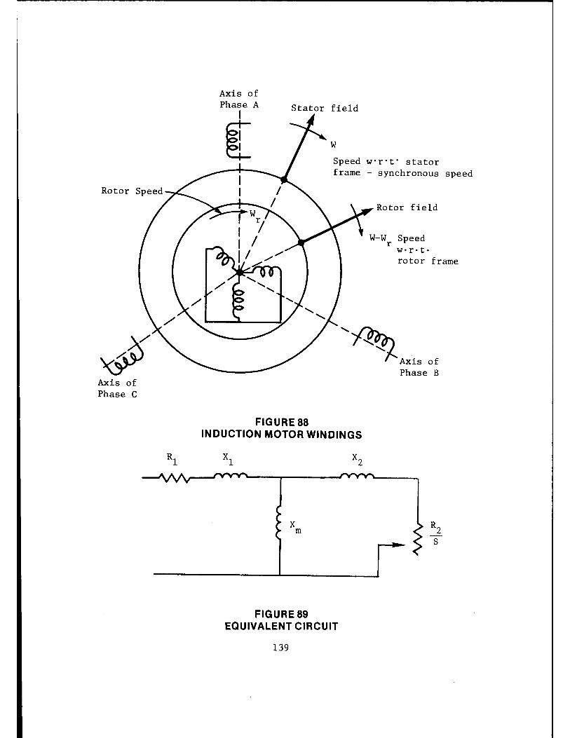
Rotor Speed
Axis of Phase C
Axis of Phase A
I Stator field
{ Speed w·r·t· stator frame - synchronous speed
FIGURE 88 INDUCTION MOTOR WINDINGS
X m
FIGURE 89 EQUIVALENT CIRCUIT
139
Rotor field
W-W Speed r w•r•t• rotor frame
-s
The torque and primary current variations with slip are shown in
Figure 90. Certain characteristics of the motor operation are evident
from this torque-speed curve.
For rotor speeds between zero and the synchronous speed, the
torque and the speed are both positive, thus resulting in a motoring
action. In this motoring region, the torque increases from its
starting value with increasing speed, reaches a maximum called the
pull-out torque, and rapidly drops to zero at synchronous speed. For
a given load characteristics, the motor operates at a speed close to
the synchronous speed (~95-99%), where the motor torque equals the
load torque - at the point P for example. This operation is very
stable because if the speed increases, the motor torque decreases
and the motor decelerates. Similarly, if the speed decreases, the
motor torque increases resulting in motor acceleration. It could also
be shown that the operation at point Q is clearly unstable. Thus for
a typical motor, the slip for the maximum torque could be in the range
0.1-0.2, and the normal full load slip could be in the range of
0.01-0.05 per unit, i.e. 1-5 percent. Thus an induction motor is
essentially a constant speed motor.
When the rotor speed is more than the synchronous speed, i.e., for
netagive slip values, the torque produced is negative, becoming a braking
torque. This mode of operation is regenerative braking. In this opera
tion, the motor is driven by the load (a vehicle going down a grade,
for example) and the kinetic energy of the load is converter to electrical
energy that is fed back to the three phase source connected to the primary.
Also, for negative rotor speeds - rotor speed in a direction opposite
to that of the rotating field - the torque is still positive, thus
opposing the rotor motion. This braking action is called "plugging".
In this operation, the kinetic energy of the load and the rotor is
wasted as heat in the rotor circuit. The primary winding continues to
draw heavy current from the supply.
140
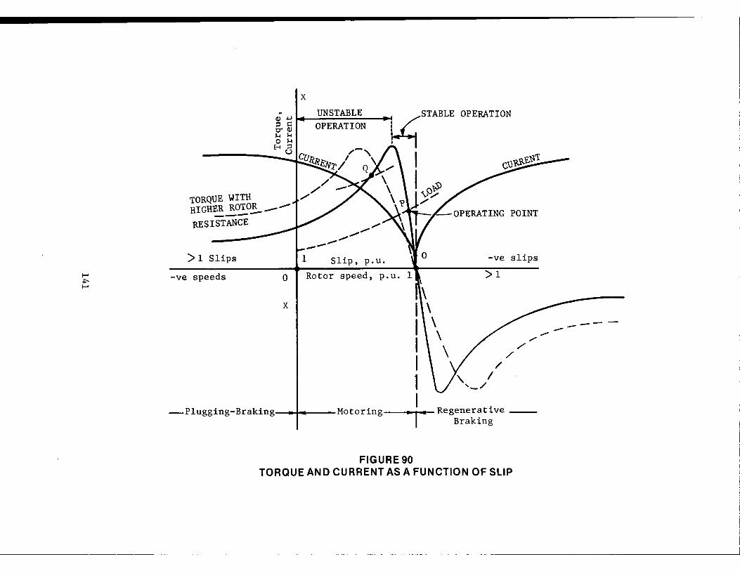
I-' .i:--1-'
X
.. I UNSTABLE Qj+J.. ..I g. ~ OPERATION I-< I-< 0 I-< E-4:::,
u
TORQUE WITH HIGHER ROTOR ---------RESISTANCE
> 1 Slips
-ve speeds 0
X
---,...,,.,,. --
1 Slip, p.u.
Rotor speed, p.u. 1
-Plugging-Braking •I• Motoring
FIGURE 90
I ' I ' I ' I '\
OPERATION
-ve slips
>1
/
' I .... _/
/
.,,,./
I 1 I Regenerative __ _
Braking
TORQUE AND CURRENT AS A FUNCTION OF SLIP
--------- -
The variations of the efficiency and the power factor of the
motor with slip are shown in Figure 91. Copper losses in the stator
and the rotor and iron losses in the stator core are the major loss
components. Iron losses in the rotor core are usually small because
the rotor carries slip frequency currents and fluxes. The power factor
depends on the airgap and the leakage reactances of the primary and
the secondary circuits.
2.3 Speed Control of Induction Motors
It can be seen from the very steep characteristics in the stable
region of Figure 90, that the induction motor is basically suitable for
a constant speed operation. The stable region can be extended by
adding external resistances in the rotor circuit. However, this is
possible only for a wound rotor motor and is clearly impossible for
a squirrel cage motor. Also, the torque can be reduced by reducing
the applied voltage. But any variable speed operation for a constant
supply frequency is possible only at increased slip and hence at
reduced efficiency. Hence, the most efficient method of speed control
requires a variable voltage variable frequency (VVVF) supply where
the speed can be controlled by changing the frequency and the torque
can be controlled by changing the voltage.
The necessity of a VVVF source for efficiently controlling the
speed of an induction motor was realized long ago, but it was not
economically feasible before the introduction of power semiconductors.
For small power applications and other applications where efficiency
considerations were not important, voltage control methods using magnetic
amplifiers, thyristors or series/parallel winding connections were
developed. For restricted speed control, pole changing motors or
pole amplitude modulation techniques were also developed. However,
none of these methods are suitable for the control of vehicle propulsion.
142

1.0
~~
0.8 /
V ~ POWER FACTOR
""ii v~ J 0.6
_,,,,,., V /" _....
l---" ~ V ---- ~
0.4 EFFICIENTYI'-- /
~ V
0.2 / /
v~ /
/
0 0.2 0.4 0.6 0.8 1.0
SPEED, p.u.
FIGURE 91 POWER FACTOR AND EFFICIENCY OF INDUCTION MOTOR
143
With a VVVF source, one can change the synchronous speed, and
hence the operating speed of an induction motor, by simply changing
the frequency of the source. The airgap flux of the motor can then be
controlled by changing the source voltage or by changing the number
of turns per phase in the motor, if possible. The operating principle
of this method of speed control can be explained with the help of
Figure 92. A typical torque-speed characteristic required for traction
application is shown. The motor is operated with a constant flux and
a constant current so that a constant torque is produced at all speeds
up to the base speed. The airgap flux can almost be held constant by
having a constant voltage/frequency ratio. Beyond the base speed, the
voltage is held constant while frequency is increased. The airgap flux
and thus the pull-out torque of the motor are reduced. A constant-current,
constant-flux, constant-torque operation (Mode A) is possible up to
higher speed for braking than for motoring. Hence, high braking torques
are possible at high speeds.
It should be pointed out here that the induction motor can operate
only at a lagging factor. This has an important impact on the design
of the VVVF source. In general, it is possible to use either line
commutated or forced commutated VVVF designs. The line commutated equip
ment is cheaper and has better fault characteristics than a forced
commutated one. However, line commutation is possible only with leading
power factor load. The induction motor, therefore, requires a forced
commutated VVVF design. The static power converters are discussed in
detail in Appendix B.
2.4 Advantages and Disadvantages
Suitability of the induction motor for propulsion of a transit
vehicle can be summarized as follows:
144

r«>DE A .. , .. MODE B
I r\ ,-...._ .,..........._~ I
t MODE A • INCREASING VOLTAGE
I- • INCREASING FREQUENCY en :::, • CONSTANT FLUX a: • CONSTANT CURRENT :c ... ... - MODE B
• CONSTANT VOLTAGE INCREASING FREQUENCY DECREASING FLUX
I ___, I ____, I I I ' ' '\. uJ => CT a:: 0 ... a:: C ...
I-' i .i:--\J1 I I \ \ IBASE
C) DESIGN z ... ~ cC a: CQ
t---\-rt-:,t-~·K/ ~ -l
--I ;' , ..-1 - _,..
" I -r«>DE A -,- MODE B
FIGURE 92 SPEED CONTROL FOR TRACTION APPLICATIONS

Advantages
• A very simple, rugged traction motor.
• High power density for weight and volume. and hence a light motor.
• High voltage and high speed operation is possible.
• Inherent tendency to control wheel slip.
• Regenerative braking without contactors
• Low initial and maintenance costs as compared to a de motor.
Disadvantages
• Requires a variable-frequency, variable-voltage power source for speed control. This results in high initial cost for the total system at this time.
• If more than one motor are used in parallel, wheel diameters need to be maintained to close tolerances.
146
3.0 THREE PHASE SYNCHRONOUS MOTOR
The operating principle of different types of synchronous motors
can best be explained with the help of a machine configuration shown
in Figure 93. Consider a three phase stator winding similar to that
of an induction motor. This winding, when excited, creates a rotating
magnetic field. This field is sinusoidally distributed in space and
rotates at a speed determined by the supply frequency. Also, consider
a salient pole rotor structure having two axes of symmetry - the polar
axis or direct axis d and the interpolar or quadrature axis q. Because
of this saliency, the magnetic flux paths have different permeances
in these two axes. The rotor is shown carrying a field winding. When
excited with a direct current, it creates a magnetic field which is
centered on the direct axis and is stationary with respect to the
rotor surface. If this rotor rotates at the synchronous speed, the
rotor field is then stationary with respect to the stator field and
an electromagnetic torque is produced. A resultant average torque
can be produced only at synchronous speed and hence these motors are
called synchronous motors.
3.1 Operating Characteristics
The airgap flux produced by the currents in the armature
(i.e., stator) winding is called the armature reaction. Since the
analysis of this armature reaction involves the rotor saliency it can
be done by resolving the armature reaction flux into components
along the rotor d-q axes. The armature currents are also resolved
into two components. The direct-axis component id causes an armature
reaction centered on the direct axis, with a reactance Xd' called the
direct axis synchronous reactance, associated with it. The quadrature
axis component i causes the armature reaction to be centered on the q
quadrature axis, with a reactance X, called the quadrature axis q
synchronous reactance, associated with it. The component Xd is
usually larger than Xq since the airgap under the direct axis is smaller
than that under the quadrature axis.
147
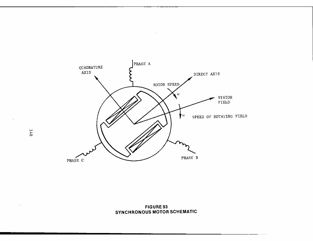
I-' ~ 00
QUADRATURE AXIS DIRECT AXIS
STATOR FIELD
w SPEED OF ROTA1ING FIELD
FIGURE 93 SYNCHRONOUS MOTOR SCHEMATIC

For a synchronous motor, the terminal voltage Vt and the excita
tion voltage Ef induced by the field winding are related as follows
(the armature resistance is assumed to be zero):
' X I J q q
This is a phasor equation that shows for a constant magnitude of the
terminal voltage Vt and of the armature current Ia' the field excitation
voltage Ef - actually the field current If - can be used to control the
power factor of the motor. This is illustrated in Figure 94. The
power factor angle~ between V and I as well as the power angle o t a
between Ef and Vt are both shown. An underexcited motor operates with
a lagging power factor and an overexcited motor operates with a leading
power factor. As mentioned earlier, less expensive thyristor power
converter equipment can be used to control a leading power factor load.
The power developed by the motor can now be obtained with the help
of the phasor diagram of Figure 94(b) as follows:
p =
-( - V Cos°) C'
Sin
') t • Vt Sin o + Vt Cos o
Xd X q
=(\E' 1 2
(x: x:) Sino + -v Sin 26 2 t
It should be seen here that the first term represents the power
due to field excitation whereas the second team represents the power
independent of excitation and due only to the rotor saleincy - i.e. the
power due to reluctance torque. The reluctance torque is produced
because of the difference in reluctance under the direct and quadrature
axes. The power expression can, therefore, be rewritten as:
149

d-axis I I
-j X I q q
1.,.::; ........ ,.._.,__-'-___ .._."'" _____________ ----- q-axis
(a) Underexcited motor, lagging power factor
d-axis
Id
I I I I I
a
-j X I q q
Ef 11i:::::;:___.-..J.---L.---------'-------t►----- q-axis
I q
(b) Overexcited motor, leading power factor
FIGURE 94 SYNCHRONOUS MOTOR PHASOR DIAGRAMS
150

p = Pf Sin 6 + P Sin 26 m rm
Where Pf and P represent the m,1ximu111 val111':; ol ti)(' powl'r d1u• to llw m rm
field excitation and reluctance v:ir i :1l i 011 1·(•:;p(•1· I i v1· I y.
3. 2 Types of Synchron0t~s __ M_o L_o r:;
on whether both Ll1l' fi.-ld t'x(·il:111"11 1,,1,111(• :111d llw J(•l1wl:11w(• l11rq111·
:ire pre:-a.•nt, dt'IH'1Hli11g 011 llw 11wllifld:; .. 1 ,-,,,,,, ,.,.,-11:il io11.
• l)ouh Iv ,·x,· I l l'd 111011ll·:; ('l'lll':.1· 1111,1 01·:; l1:1v,· :11111:1 r 111·,. :11,d ! i ,. ! rl t•x,·i[;Jt 1011 ;1111I 111·111·1· lwo lo1·q1H· 1·0111po111•11f:;. <:yl i11rlr i•·:il c,111:;tnll'I 11111 li:1:; j•,r1•;1l ly 1·(•d1w1•d 1·(•l1wl:11w•· l11n1111·).
l't·n11;111,·111 111:1r,111·I 1·:~c i I :il _i 011 l~ot,11· rit•ld windings supplied tlin1111•.l1 :;I ipri11)',:, Roto1· rit•ld supplil'd Llirougli ;1 rot:1Li111•. lr:111slor1111·r ll0111opol:1r inductor 111;l('lii11t• Lundell/Rice 111ad1 i Ill'
• Singly excited or reluctance motors (These motors hnvt• no field excitation and hence have only the reluctance torque).
Synchronous reluctance Sub-synchronous reluctance motor, i.e., a Vernier motor
The above configurations will now be described.
3.2.l Permanent Magnet Synchronous Motor
The principle of operation of this motor is the same as described
l'arlier. However, the rotor magnetic field is created by using pe::nnanenl
nmgnets instead of electromagnets. The rotor excitation is thus con-
tactless and hence there are no sliprings or brushes to wear. The
field, however, cannot, be easily controlled. Hence, weak-field con-
ditions cannot be easily achieved for traction applications. It
should also be remembered that as long as the rotor is driven, the
pennanent magnet excitation will induce armature voltages and hence
these motors cannot be deenergized. Thus, if the armature winding
of a permanent magnet sychronous motor develops a fault, the motor can
151
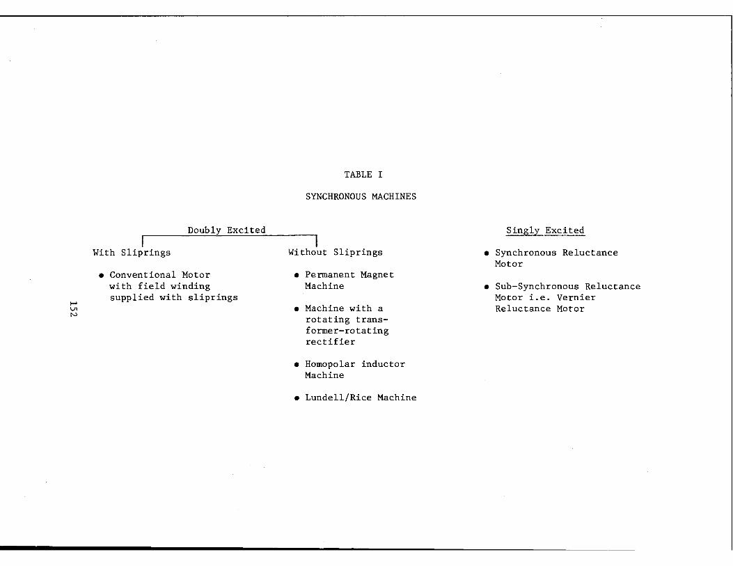
~ Vl N
Doubly Excited
With Sliprings
• Conventional Motor with field winding supplied with sliprings
TABLE I
SYNCHRONOUS MACHINES
Without Sliprings
• Permanent Magnet Machine
• Machine with a rotating transformer-rotating rectifier
• Homopolar inductor Machine
• Lundell/Rice Machine
Singly Excited
• Synchronous Reluctance Motor
• Sub-Synchronous Reluctance Motor i.e. Vernier Reluctance Motor
be burned out if the rotor is allowed to rotate, even if the motor
is disconnected from its converter. In a multi-car vehicle consist,
therefore, if one motor develops a fault, it has to be mechanically
decoupled before the vehicle is moved.
With improved, inexpensive permanent magnet materials, these
motors will, no doubt, be increasingly used for various applications.
3.2.2 Rotor Field Supplied Through Sliprings
This is the most connnon method of supplying field winding of a
synchronous machine. The rotor winding terminals are brought out
to two sliprings on the shaft and the de field current is fed through
a set of brushes. The field can then be controlled quite easily. The
brushes, of course, need regular cleaning.
For application in rail propulsion, this motor has very little
to offer. It is big and heavy compared to a squirrel-cage induction
motor and it still has a brush-gear similar to a de motor. Simple
and cheap solid state converter circuits can, however, be used with a
synchronous motor. In some countries, such as the Soviet Union for
example, this could be an overriding consideration because the solid
state technology is not as advanced. This can possibly explain their
interest in continued development of a propulsion system using slip
ring synchronous motors for their VL80 type locomotive.
3.2.3 Rotor Field Supplied Through a Rotating Transformer
The rotor field can be supplied without sliprings (contactless)
and can still be controlled if one uses a rotating transformer and
rectifier equipment as shown in Figure 95. The shaft of the synchronous
machine carries the secondary of a three phase transformer. The induced
voltage in this winding is rectified by means of a rectifier circuit,
also carried on the shaft. This rectified voltage is used directly to
153
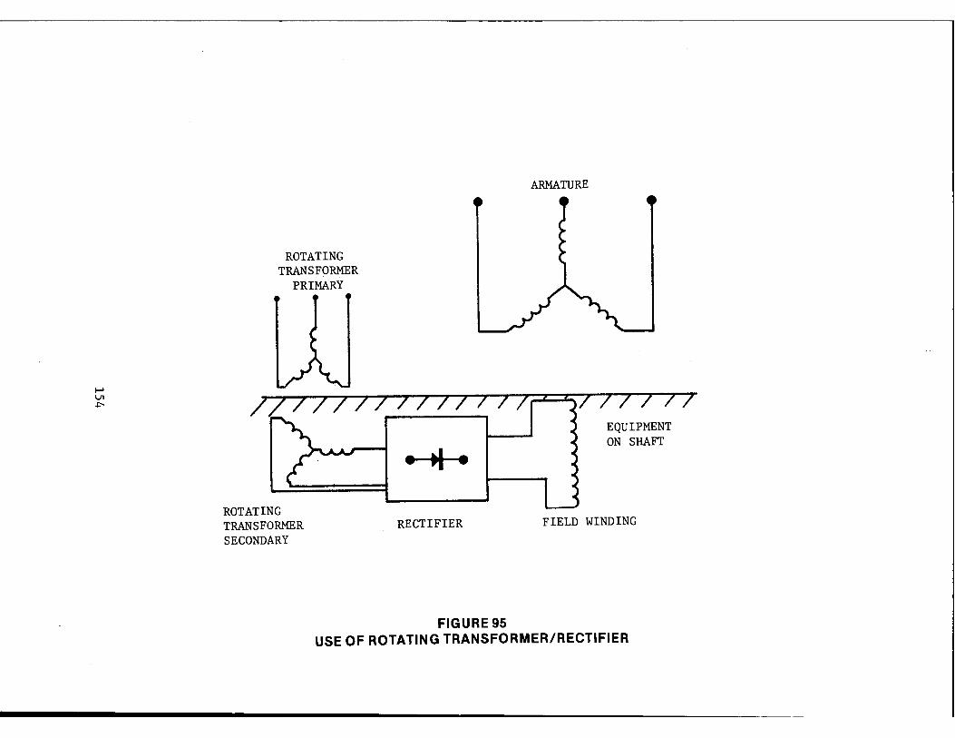
f-' \J1 .i:--
ROTATING TRANSFORMER
PRIMARY
ROTATING TRANSFORMER SECONDARY
. .. . RECTIFIER
FIGURE 95
ARMATURE
EQUIPMENT ON SHAFT
FIELD WINDING
USE OF ROTATING TRANSFORMER/RECTIFIER

excite the rotor field. There is thus no contact between the stator
and the rotor circuits and the energy to excite the field is obtained
from the primary of the rotating transformer. Such systems are currently
in use for several industrial applications.
A propulsion system for urban rail application using such a
motor is described at greater length in Section 5 of this report.
3.2.4 Synchronous Reluctance Motor
This motor is a singly excited sychronous motor, wherein torque
is generated because the airgap reluctance is a function of rotor
position. The rotor carries no windings or permanent magnets but
the airgap reluctance is different for the d-axis and the q-axis. A
reluctance torque is, therefore, generated given by the second term
of the power equation given previously. The essential features of
the machine are shown in Figure 96.
It should be noted here that the reluctance distribution along
the rotor periphery rotates at an angular velocity equal to the rotor
velocity, i.e., when the rotor moves through an angle 8, the reluctance
distribution also moves through an angle~ equal to 8. Thus the rotor
rotates at synchronous speed, keeping the rotor flux stationary with
respect to the stator flux.
The reluctance motor, being a singly excited device, cannot
operate at a leading power factor and, in fact, has a very poor power
factor. This motor is thus of little use in transportation applications.
The rotor construction, however, is simple and rugged. This motor,
therefore, is frequently used for applications in control circuits.
3.2.5 Vernier Reluctance Motor
A vernier reluctance motor is another singly excited machine in
which a reluctance torque is generated because the airgap reluctance
155

is a function of the rotor position. However, in this machine, if
the rotor moves through an angle 6, the configuration of the rotor
causes the reluctance distribution to move through an angle~.
different from e, but always a constant multiple of 6 (~ = N • 8) as
shown in Figure 97. This means that the rotor field can rotate at
synchronous speed, remaining stationary with respect to the stator
field, if the rotor rotates at a sub-synchronous speed given by
rotor speed 1 N
synchronous speed
The factor N depends on a particular design. For example, consider
a doubly slotted structure as shown in Figure 98. Here the slot pitches
are chosen such that
A s
A r
4 3
where A and A are the stator and the rotor slot pitch respectively. s r
The maximum permeance ( minimum reluctance) along the rotor periphery
is obtained where the stator and the rotor teeth are opposite each
other as shown. Now if the rotor is moved through half the stator
slot pitch, the permeance/reluctance distribution moves through two
stator slot pitches, as shown in Figure 98(b). This means that if the
rotor field rotates at the synchronous speed, the rotor will rotate
at l/4th the synchronous speed.
For a vernier motor it can also be shown that the mechanical torque
developed by the motor is N times the reluctance torque given previously,
i.e.,
T = N • T mech rel
156

Rmin R Rmin max I I I I 'd I q
I I
J I I I
I __,I.,, r--d •q
I I
FIGURE 96 SYNCHRONOUS RELUCTANCE MOTOR
I I
Id I
I e ~/ ROTOR DISPLACEMENT
I I
I / ,, .....
<P = N • 8
.....
I I
d
R-airgap reluctance
'DISPLACEMENT OF RELUCTANCE DISTRIBUTION
FIGURE 97 VERNIER MOTOR
157

I-' V, 00
Pmax I
I I I
1lJ J
I I I I
Pmax
LJ I I w I I I I I I I I
I I I
FIGURE 98(a) DOUBLY SLOTTED STRUCTURE OF VERNIER MOTOR

I-' \J1 \.Q
PERMEANCE WAVE MOVES TWO STATOR SLOT PITCHES
I I I
I ROTOR MOVES HALF I I I STAT~, SLOT PITCH Ip I p max max
I_..... ___ I_ -- --'
l i I i I I I ! I I I I I I !I - I I
l' 11111 Iii 1111111!11111 ROTOR MOTION----
F!G!JRE 98(b) DOUBLY SLOTTED STRUCTURE OF VERNIER MOTOR
Now, since
rotor speed 1 N
synchronous speed
the vernier motor behaves like a built-in electromagnetic reduction
gear.
Experimental investigations on laboratory models have shown that
slot shapes and slot combination need to be optimized for obtaining
a higher power density, and even then the power factor is very poor.
These motors also tend to be noisy because of the presence of a
doubly slotted structure.
If such a motor is used for traction applications,it could possibly
eliminate the need for a gear box and the motor could be directly
built on the shaft. The power factor will, most probably, have to be
improved by using static capacitors in order to reduce the inverter
cost. Its suitability for urban rail systems can be evaluated only
after a preliminary design of a total system including the motor and
the converter.
3.2.6 Other Doubly Excited Configurations
We have so far seen three types of doubly excited synchronous
motors. The permanent magnet motor cannot be easily operated under
weak field conditions and for transit applications and it needs to
be mechanically decoupled if fault conditions develop. The motor
with sliprings has brush wear problems and a motor with a rotating
transformer is quite a complex system. There are, however, some other
configurations in which it is possible to create rotor field without
bringing the field current into the rotor. In these configurations,
the armature and the field winding are both on the stator and the field
flux is made to go through rotor structure by developing special topo
logies. These will be described in this section. The reader should
be cautioned here that these are basically 3-dimensional topologies
160
and only an attempt can be made to explain these with the help of some
illustrations. The advantages and the limitations of these motors will
be presented, but any detailed discussion is beyond the scope of this
report.
3.2.6.1 Homopolar Inductor Motor
Consider a machine shown in Figure 99. It essentially consists
of two rotor cores, and a common field winding. The salient poles of
the rotor cores 1 and 2 are shown in Figure 100. It can be seen that
the poles are shifted by a pole pitch. The flux density distributions
along the airgap around the rotor cores is therefore as shown in
Figure 101.
The field winding, when excited, creates an airgap flux distribu
tion as follows:
a) The flux enters the rotor on one side, say core 2, goes to core 1 through the central shaft, and returns to the yoke from core 1.
b) Along the periphery of core 1 or core 2, the flux is all unidirectional, and hence the name, "homopolar motor". The flux distributions will depend on the topological constants such as the pole arc-to-pole pitch ratio, interpolar gap, etc.
The armature winding reacts with the sinusoidal component of the rotor
field to create an electromagnetic torque. The homopolar machine is
usually heavy because the magnetic structure has to handle the average
field flux which does not contribute to the thrust. The alternating
component of the airgap flux depends directly on the difference
(B - B . ). The maximum flux density is, of course, limited by max min
the saturation level and the minimum flux density depends on the
leakage characteristics. The design of such machines is quite
complex compared to say, an induction motor design, and one has to
optimize the design considering various parameters such as the pole
arc/pole pitch ratio, ac flux/average de flux ratio, etc.
161

f-1
°' N
FIELD WINDING---.. .--- STATOR CORE
YOKE
ROTOR
r:~~\ I I I I ,,;,--~ \ \ ~!h;=---=~•~!!!!!~ii;;=--=~r.. I I \ \ I I , \ 188 89 ,,,,
\ .. ------------------ 1, ' '... ,; ', ____________________ ~
' ~ .... - - - - - - - - - - - - ----- _,
FIGURE99 HOMOPOLAR INDUCTOR MOTOR
AC WINDING
SHAFT
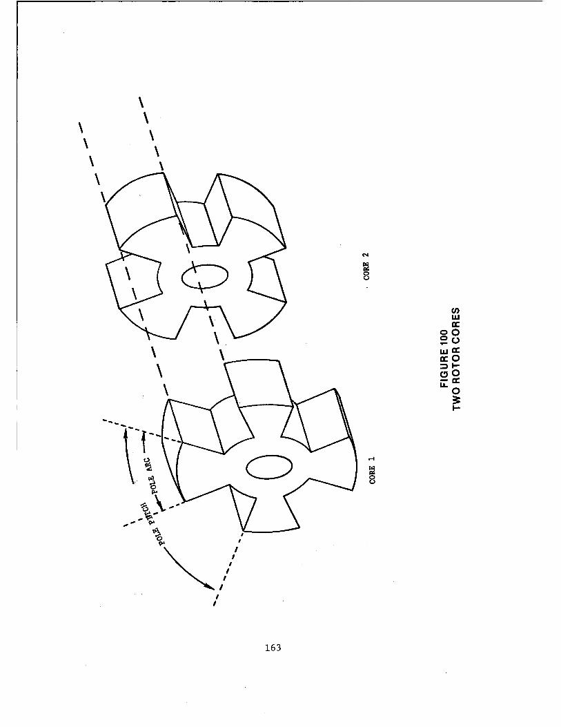
\ \ \ \ \
\ \ \ \ \
I I
163
N
....
en w a:
oo ~o w a: a: 0 ~ 1-c, O U: a:
0 31: I-

f--'
"' .i::--
BMAX
BMii.~
0 B~UN
_BMAX
CORE 2
8 •
FIGURE 101 AIRGAP FLUX DENSITY DISTRIBUTIONS

•
As can be seen, this machine has a very simple, rugged rotor
like a squirrel cage motor and it can also operate at a leading power
factor. Large weight, volume and higher commutating reactance are
some of the disadvantages of this motor. A high commutating reactance
results in an expensive converter design. This commutating reactance
could possibly be reduced by introducing some damping circuits to
reduce the effects of high field leakage reactance.
In short, the homopolar inductor motor has some significant
characteristics to make it a useful traction motor. However, there
is a need to further evaluate motor designs for traction application
before a judgement can be made on this issue.
3.2.6.2 Lundell/Rice Motor
These special motors are heteropolar synchronous machines where the
armature and the field winding are placed in the stator and the rotor
field is created by properly directing the field flux through the rotor
structure. The rotor structures of these motors are quite complex, but
there are no brushes or the sliprings to wear.
Consider for example a motor shown in Figure 102. It is
commonly known as a Rice machine. The two windings, the magnetic
and the non-magnetic parts of the structure are marked. One side
of the rotor acts like a south pole and the other side like a north
pole. The field flux path is as follows:
The yoke+ the rotor on one side (right in Figure 102) + a rotor
pole ➔ the armature+ the next rotor pole+ the rotor on the other
side (left in Figure 102) + back to the yoke.
The field flux thus covers four airgaps: two main airgaps
between the armature and the field poles and two parasitic gaps
between the yoke and the shaft. It should also be noted here that
165

f-'
°' °'
FIELD COILS
NON MAGNETIC INSULATOR
ARMATURE
._ ) FLUX PATH
STATOR ASSEMBLY
FIGURE 102 RICE MOTOR
MAGNETIC HOUSING AND END BELL

the flux does not cross between the rotor poles but goes through the
armature because the magnetic reluctance of the path through the
armature is quite small compared to the gap between the rotor poles.
A second possible topology is shown in Figure 103. It is known
as a Lundell machine. The field winding is fixed to the stator
frame, but it is housed inside the rotor, thus shortening the path
of the field flux. For a six-pole construction of Figure 103, the
shaft and the three south poles form one structure and the three
north poles are connected to the shaft with a non-magnetic separator.
The north poles extend out and over the field winding. The flux
path is as follows:
The yoke ➔ a rotor north pole+ the armature ➔ the next south
pole (on both sides) ➔ the shaft ➔ the yoke.
It should also be noted here that the field flux crosses two main
airgaps and two parasitic airgaps as in the Rice motor described
above. This Lundell motor cannot be designed for very high speeds
because of the dynamics of the complex rotor structure. Also,
because of the high leakage fluxes, it has high commutating reactance,
thus needing expensive inverter. Here again, a damping circuit can
possibly be introduced to reduce the commutating reactance.
The Lundell/Rice motor has several significant characteristics
to make it a potentially useful traction motor. The suitability of
these motors for rail propulsion, however, can be evaluated only
after a total system design is worked out.
3.3 Advantages and Disadvantages
The suitability of different types of synchronous motors can be
summarized as presented in Table II.
167

f-'
°' 00
FIELD YOKE
NON MAGNETIC HOUSING ARMATURE WINDING
STATOR ASSEMBLY
~~~~f;~~~§~=-- NORTH POLE RING , _____ NONMAGNETIC INSUL
. _,,r-SOUTH POLE
FIELD COIL
~ / SHAFT tt««A
FLUX PATH
FIGURE 103 LUNDELL MOTOR

f-'
"' '"'
Doubly Excited
Advantages
TABLE II
SYNCHRONOUS MOTORS
Advantages
Singly Excited
• Unity or leading power factor operation possible
• Gear may be eliminated by a vernier reluctance motor
• Cheap line commutated inverters can be used
• Motor-inverter optimization possible
Disadvantages
• Large, heavy, expensive motor
• One inverter per motor essential
• Special starting methods may be required
Disadvantages of Individual Types
• Permanent magnet motor
Disadvantages
• Poor power factor
• Heavy motor
- weak field conditions are difficult if not impossible
- needs to be mechanically decoupled in case of a fault
• Slipring motor - brush wear & associated maintenance
• Motor with a rotary transformer - overall system complexity
• Inductor/Lundell/Rice motor - high commutating reactance

APPENDIX II
POWER CONVERSION DEVICES
1.0 STATIC CONVERTERS
The thyristor or semiconductor controlled rectifier (SCR) was
developed in the late 1950's and became commercially available in
1960-61 in the ratings of approximately 200A and 1000V. Initially
some difficulties were encountered in thyristor applications because
the device itself was not fully understood. After these difficulties
were surmounted, however, the thyristors gained wide acceptance very
rapidly, and over the last decade, the growth of power electronics
has been phenomenal. The earlier control components - thyratrons
mercury-arc rectifiers, magnetic amplifiers, etc. - were superseded
by thyristors and quickly became obsolete. Various types of solid
state power converters were developed which could convert power from
a fixed voltage de or ac source to a variable-voltage, variable
frequency ac or variable-voltage de power. Basically, a chopper is
a de-to-de converter whereas an inverter is a dc-to-ac converter.
171

2.0 THE CHOPPER
The chopper is a de-to-de converter which varies the average
value of the direct voltage applied to a load. In general, there
are two classes of chopper circuits - a step-down chopper, where the
load voltage is less than or equal to the supply voltage, and a step
up chopper, where the load voltage is equal to or more than the
supply voltage. There are, of course, several types of chopper
configurations in each of the above classes, depending on the commu
tation circuits used. Also, several choppers can be used to obtain
a 4-quadrant circuit, i.e. circuit capable of reversal and regenera
tion.
The operating principle of a step-down chopper is shown in
Figure 104. It shows that the chopper applies a continuous sequence
of unidirectional voltage pulses to the load, the magnitude of the
pulse being equal to that of the supply voltage. The width of the
voltage pulse t and the period T of the pulses can be controlled by on
the chopper circuit.
Under ideal conditions
V 0
t on T
• V
and hence, the average load voltage V can be varied in the following 0
ways:
a. Pulse-width modulation, where t is changed while Tis held constant. on
b. Frequency modulation, where t is held constant while on Tis changed.
c. Combined pulse-width and frequency modulation.
In practice, the output voltage waveform of a chopper is different
from the ideal one shown in Figure 104 but the essential characteristics
of a chopper can be explained more easily with the idealized model.
172

t-' -..J uJ
+ ----
V CHOPPER
V 0
- --
_I -__I I ___ I I ___ I t Vo l V
... ... I t 1 on
.-
FIGURE 104 OPERATING PRINCIPLE OF A CHOPPER
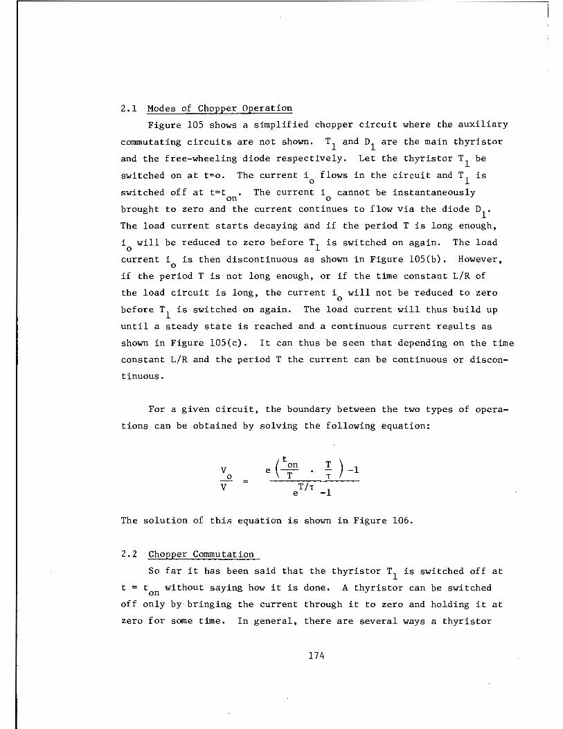
2.1 Modes of Chopper Operation
Figure 105 shows a simplified chopper circuit where the auxiliary
commutating circuits are not shown. T1 and n1
are the main thyristor
and the free-wheeling diode respectively. Let the thyristor T1 be
switched on at t=o. The current i0
flows in the circuit and T1
is
switched off at t=t The current i cannot be instantaneously on o
brought to zero and the current continues to flow via the diode n1
.
The load current starts decaying and if the period Tis long enough,
i will be reduced to zero before T1 is switched on again. The load 0
current i is then 0
discontinuous as shown in Figure lOS(b). However,
if the period T is not long enough, or if the time constant L/R of
the load circuit is long, the current i will not be reduced to zero 0
before T1
is switched on again. The load current will thus build up
until a steady state is reached and a continuous current results as
shown in Figure lOS(c). It can thus be seen that depending on the time
constant L/R and the period T the current can be continuous or discon
tinuous.
For a given circuit, the boundary between the two types of opera
tions can be obtained by solving the following equation:
V 0
V
The solution of this equation is shown in Figure 106.
2.2 Chopper Commutation
So far it has been said that the thyristor T1
is switched off at
t = t without saying how it is done. A thyristor can be switched on off only by bringing the current through it to zero and holding it at
zero for some time. In general, there are several ways a thyristor
174

i 0
i g
+
V
i _..s i
Tl
g
iD
Dl
i 0
+ L
R 0
+v - C
o.,__ ___ ...__ ________ ___..,__ __ _._ _____ ,. ton T T + t t
i 0
tl t
V V V V
0 C
t
i g
t T T + t 2T t
Imax
Imin
t
V V V
o.
FIGURE 105 t
CHOPPER CIRCUIT AND ITS RESPONSE
175
(a)
(b)
(c)

can be switched off - a transfer of load current from one thyristor to
another is called "commutation":
• The thyristor current goes through zero because of the voltage across it reverses (line commutation) or because the load current goes through zero with capacitive load (load commutation), and
• A current in a direction opposite to the load current is forced through a thyristor (forced commutation) by using auxiliary circuits.
These commutation methods will be discussed in detail later, but one
method commonly used in chopper designs is explained in Figure 107.
When T1
is triggered on, the recharging thyristor T3
is also switched
on so that the commutating capacitor C reverses its polarity. So
while T1 is conducting, the capacitor C is charged with plate "a"
having a positive potential. Now if the commutating thyristor T2
is
switched on, the capacitor C is connected in parallel with T1 , and
the load current is transferred from T1
to T2 . Also, the capacitor
C gets charged in the opposite direction, with plate "b" being positive.
T2 then switches off and the free wheeling· diode n1
begins to conduct
and the voltage across the load and the load reactor drops to zero.
The main thyristor T1
(and T3
) can be switched on again.
Although the load current in a chopper can be continuous because
of load inductance and the free-wheeling diode, the current drawn from
the supply is in the form of pulses of the duration oft No current on
is drawn from the supply during the 'off' period. An L-C filter is
usually used to smooth out the supply current. This is shown in Fig
ure 108.
2.3 Multi-Phase Choppers
Several choppers can be used in parallel to feed a common load as
shown in Figure 109. Such a circuit is commonly known as a multi-phase
chopper. The voltage waveforms of a three phase arrangement are shown
176

:> ...._ C
:> ~
0 H c--<
~ c--< :::i p... c--< :::i 0
V +
1.0
0.9
0.8
0. 7
0.6
0.5
0.4
0.3
0.2
0.1
0
0 :> ...._
0 :>
0 t /T 1.0
on
T - ➔ 00
T
0.1 0.2 0.3 0.4 0.5 0.6 0.7 0.8 0.9 1.0
CONDUCTION RATIO, t /T on
FIGURE 106 DIFFERENT MODES OF CHOPPER OPERATIONS
b a
+ C
FIGURE 107 CHOPPER COMMUTATION
177
LOAD
Tl - MAIN THYRISTOR
T2 - COMMUTATING THYRISTOR
T3
- RECHARGE THYRISTOR

f-' --.J 00
+
V
i s .. 'ff' l 1
c + -,- -
i s
ich ..
V I
C
Chopper I
ich
FIGURE 108 FILTER RESPONSE
I ILOAD
VC
i C

REACTORS
__ n_----+-rL
FIGURE 109 MULTI-PHASE CHOPPER
179

in the figure. The frequency of the load voltage can be seen to be
three times the frequency of the individual chopper. Moreover, each
chopper has to handle one third the load power. Also, the three
reactors can be wound on a common iron core so that the fluxes due to
the average current are cancelled out and hence, do not saturate the
core. The harmonic content of the supply current can also be reduced
by properly phasing the choppers with realtion to each other. Two
phase choppers are commonly employed for control of de traction motors.
180
3.0 INVERTERS
It has been generally accepted that the most efficient method of
speed control of ac drives is to use a variable-voltage, variable
frequency (VVVF) ac supply to control the ac motor. With the advent
of thyristors, it is now posible to convert power from a de source to
a VVVF ac power at reasonable costs. Inverters are a class of such
circuits for dc-to-ac conversion. There are several types of inverters,
and different types can be defined from several points of view. Depend
ing on the method of thyristor commutation - transfer of load current
from one thyristor to another - one can broadly consider three types of
inverters:
a. Line Commutated inverter: In this type of an inverter, the voltage across the thyristor reverses because of a presence of an ac line or a back-emf from the load. The thyristor, therefore, switches off when the current drops to zero. This is also called 'natural commutation' of a thyristor.
b. Load Commutated inverter: Here the current through a thyristor drops to zero because of a natural tendency of the load current to drop to zero when excited by a de source. A load with series inductances and capacitances having an oscillatory response, for example, can be controlled using a load commutated inverter. This is also called a 'natural connnutation' of a thyristor.
c, Forced Commutated inverter: Here, an auxiliary voltage source - usually a charged capacitor - is connected across a thyristor in such a way that the voltage across the thyristor reverses. The thyristor switches off and the load current can continue to flow through a free-wheeling diode connected across the load.
Out of these three types, the forced commutated and the line
commutated inverters are quite suitable for ac drive control in a tran
sit vehicle.
is1

3.1 Line Commutated Inverter
The operation of a line commutated inverter can best be explained
with the help of a 3-phase bridge rectifier circuit shown in Figure
110. Two thyristors - one odd numbered and one even numbered - conduct
at a time for continuity of the load current. The instantaneous load
voltage Vd depends on which thyristors are conducting. For example,
if T1
and T2 are conducting, Vd = Vac The instantaneous and hence,
the average output voltage can, therefore, be controlled by varying
the thyristor triggering angle. Figures 111 and 112 show the operation
of the circuit for two firing angles a= 30° and a= 150°. For
a= 30°, the average voltage is positive and for a= 150° it is negative.
It can be shown that for a 90°, the average voltage is zero. Figure
113 shows the variation of the average voltage as a function of the 0
firing angle a. It should be seen that for a< 90 , the power flow is
from the ac circuit to the de circuit and the circuit works like a
rectifier. 0
For a> 90 , however, Vd reverses and the power flows from
the de source to the ac source. This operation is called an inverter
operation.
The voltage waveforms shown in Figures 111 and 112 assume an
instantaneous commutation, i.e., the current transfers from one thyristor
to another instantaneously. In practice, however, the commutation
process is spaced over a finite time period, called the overlap period
which depends on the commutating reactance of the circuit. The average
output voltage is then less than that given by Figure 113.
It should be noted here that the commutation is achieved because
of the ac line voltage and hence, the inverter is called the line
commutated inverter. Also, the inverter operation results in a lagging
current being drawn from the ac source although the inverter supplies
real power to the ac source. This is quite clear from the phasor
diagram drawn in Figure 114 for the inverter operation with a= 150°.
182
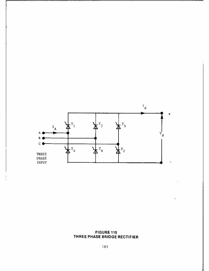
Id
+
IA Tl T3 TS
A Vd B
C
T4 T6 T2 THREE PHASE INPUT
FIGURE 110 THREE PHASE BRIDGE RECTIFIER
183

C/)
~ H c.,
~ z 0 H E-t u ;:J Q z 0 u ~ 0 E-t C/)
H ~
~ E-t
I I
I \ I\ /\ I \/\/\ 1,,,1 "'/YYX'< /\ 1\ ,\ t\ 1\ /,
I \ I ~I \/ ,,/ '/ 'v .... ___ .)',_✓ ,.,._,,. '--"' .... __ ..... ,...__..,
FIRING ANGLE a 30°
Output Voltage Vd
T . 1 1----__,I----.....J.-----------
T2
T3
T4
TS
FIGURE 111 RECTIFIER OPERATION FOR a = 30°
184

Cl)
r.:i:l H c.!)
~ :z 0 H E-1 u :::> A :z 0 u ~ 0 E-1 Cl)
H ~ :>< :::i:: E-1
I a. =150°___.J
I
Tl ._ _______ _,_ ____ ..L-___ _
T2
T3
T4
TS
T6 _________________ _
FIGURE 112 RECTIFIER OPERATION FOR a= 150°
185

1.0
0 •r-1 .µ Cl!
p::; 0 30 60 (I) 0 bO Cl! .µ r-1 0 :> r-1 tll ~
•r-1 s -0.5 ~ (I)
E-4 . CJ
I A
-1.0
120
\ \
\ \
\ \
\ \
\
', '
FIGURE 113 RECTIFIER OUTPUT
186
150 180 Firing Angle
Rectifier operation
---Inverter operation
' ' ........ --
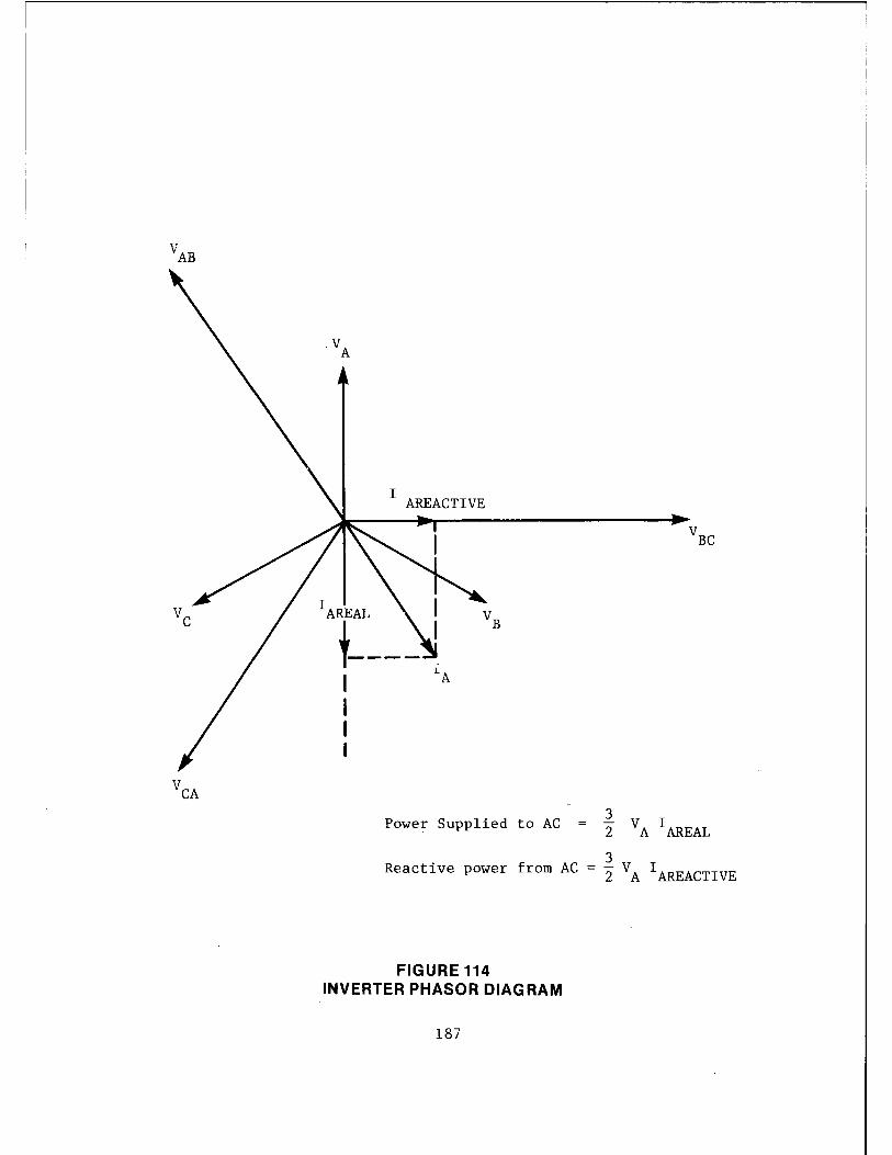
I AREACTIVE
1AREAL
t----1
I I I
3 Power Supplied to AC = 2 VA !AREAL
3 Reactive power from AC= 2 VA IAREACTIVE
FIGURE 114 INVERTER PHASOR DIAGRAM
187

This means that the ac load on the inverter must operate at a leading
power factor. An overexcited synchronous motor, for instance, can be
supplied by such a line commutated inverter.
3.2 Forced Commutated Inverter
A forced commutated inverter uses a charged capacitor to momen
tarily reverse the voltage across a conducting thyristor to switch it
off. There are several ways to use such a forced commutation, and
depending on the number of commutations required per cycle of the
output voltage, the commutation circuit requirements differ. Moreover,
the output voltage control and harmonic reduction requirements increase
the general complexity of the inverter design. A discussion of all
these inverters is clearly outside the scope of this work. However,
the basic concepts and the inverter characteristics of one type of
inverter are explained below.
3.2.1 Inverter Operation
Figure 115 shows a single phase inverter circuit which uses a
center-tapped de supply. Three phase and three phase bridge inverter
circuits can be built from this basic circuit. The main thyristors
T1 and T2 are switched on to conduct the load current during alternate
half cycles of the ac output. For a reactive load, the feedback
diodes D1 and D2 conduct for a part of each half cycle to return the
reactive power from the load to the supply. The main thyristors are
commutated by means of a commutation circuit of an inductance L, a
capacitor C and the auxilliary thyristors TlA and T2A.
Let T1 be assumed to conduct the load current and the capacitor
C charged as shown in Figure 116. Now let TlA be fired to commutate
T1 . The capacitor C now starts discharging and a current le flows
through TlA' C, Land the load as shown. This discharge current pulse
builds up and thus the current 11
through T1
is reduced.
188
When I C
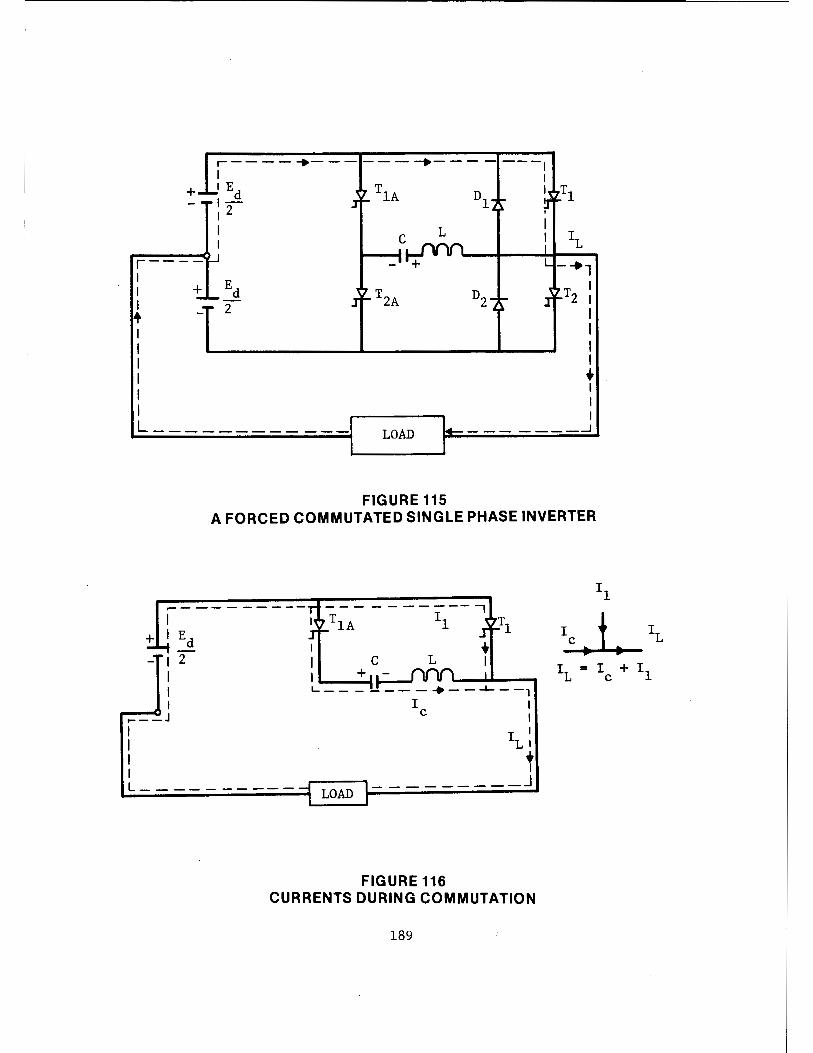
+
,--- - -.- -- --- -.- -- - ---1 I
I I Ed T I I- lA D1 ,2
I L I
r----1 I Ed I 2
-+, I
D2 T2 I
+ I I I I I I L ___________ _
LOAD
FIGURE 115
I I I I + I I I
--- ____ ...J
A FORCED COMMUTATED SINGLE PHASE INVERTER
..----------11
I + I Ed
- I 2 I
--- - ------7 TlA 11 Tl Ll.- 1
1
I
---o' ,---J I I I I L----------
L - - - - - - - -+ - - -L- - -, I I
C I
I IL I
+ I
.-------._ - - - -- - __ J LOAD
FIGURE 116 CURRENTS DURING COMMUTATION
189
IL= le+ 11

equals IL, 11 is reduced to zero. Then any excess of le over IL flows
through the feedback diode n1
• The voltage drop across n1
when it
conducts appears as a reverse voltage across T1
and turns it off.
After reaching a peak, I starts to decay and the capacitor is charged C
with polarity shown in Figure 116 (opposite to that shown in Figure
115). T2 can now be switched on, and the load current is then reversed.
The auxiliary thyristor T2A can be fired when required to commutate
T2 • The load voltage is a square wave under all conditions of loading
when the circuit is commutated only twice per output voltage cycle.
3.2.2 Three Phase Inverter Circuit
A three phase inverter circuit is shown in Figure 117. It can be
seen that the de source need not be center-tapped. The thyristors are
triggered in the order 1-2-3-4-5-6. Depending on whether a thyristor
conducts over 120 or 180 degrees in each output voltage cycle, two or
three main thyristors conduct simultaneously. It should be remembered
that at least two main thyristors have to conduct for the continuity
of the load circuit. The output voltages for these operating conditions
are shown in Figure 118. Because of the three wire system of three
phase connections, the line current and the line voltage are free of
triplen harmonics. With only two commutations per output voltage
cycle, the ac output voltage can only be controlled by controlling the
input voltage. For such an operation with varying input voltage, the
commutation networks are connected to an auxiliary de supply of fixed
voltage so that the commutating capacitor charges to this fixed voltage
irrespective of the input voltage.
3.2.3 Inverter Voltage Control
Most inverter applications require a means of voltage control.
This control may be required because of variations in the de source
voltage, regulation within the inverter, or because it is desired to
provide continuously variable voltage for the load. When the inverter
190
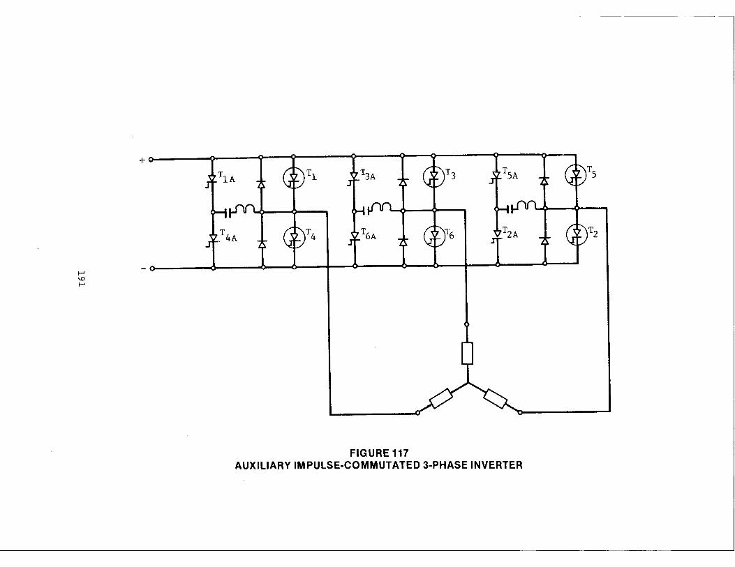
t-'
'° t-'
+o Q 9 9 'i' 'i 'i 'i 'i -,
TlA Tl T3
_T4A T4 T2A
FIGURE 117 AUXILIARY IMPULSE-COMMUTATED 3-PHASE INVERTER
T2
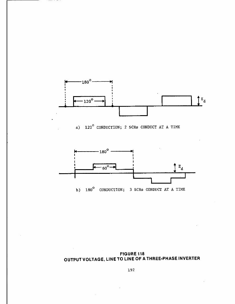
,. 180° .. , I
E1200-.1 I I I • • I I ) 1200 2 a CONDUCTION; SCRs CONDUCT AT A TIME
14 180° •I I I I I I I I F6o0 ::.j I l Ed I I
I l I
b) 180° CONDUCTION; 3 SCRs CONDUCT AT A TIME
FIGURE 118 OUTPUT VOLTAGE, LINE TO LINE OF A THREE-PHASE INVERTER
192

is used as a variable frequency - variable voltage source for traction
control, the hannonic content of the output voltage wavefonn has also
to be controlled.
There are innumerable methods of inverter voltage control, each
having many advantages and disadvantages. One can select a few of
these for a specific application depending on the power rating, the
range of voltage and frequency and the pennissible hannonic content in
the output voltage wavefonn. Finally, one particular scheme can then
be chosen depending on how each of the above relates to the "total
systems concept."
The methods of voltage control for traction application can be
divided into two groups:
as:
a. Methods using one three-phase inverter as shown in Figure 119.
b. Methods using multiple inverters as shown in Figure 120.
The circuit of Figure 119 can be operated in three different ways
a. Variable input voltage; two connnutations per cycle.
b. Fixed input voltage; four added connnutations per half cycle.
c. Variable input voltage; four added connnutations per half cycle.
The circuit of Figure 120 can also be operated in three different
ways as fixed input voltage as:
a. Four added connnutations per half cycle.
b. ~any equi-spaced connnutations per half cycle.
c. Many "progrannned" commutations per half cycle.
193
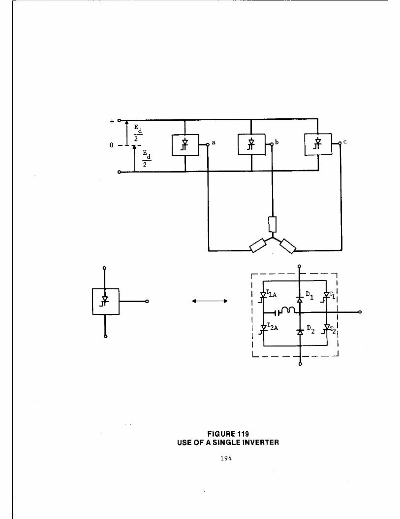
+ Ed 2 b C
0 - a
Ed 2
r---- --7 I I
I D1 I 1111 .. I
11
I I I I
I D2 ~2: I I I L ___ ___ _J
FIGURE 119 USE OF A SINGLE INVERTER
194

•• E d
2
0----;- ii- - b
,-: -------- ------- "-7 MOTOR
WINDINGS I I I I L _____ ------ ----- -----~
if - b'
FIGURE 120 USE OF MULTIPLE INVERTERS
195

3.2.3.1 Input Voltage Control: Two Commutations per Cycle
When the circuit of Figure 119 is operated with two commutations
per cycle, the instantaneous voltages of points a and b with reference
to O can be drawn as in Figure 121. The resulting line voltage between
a and bis also shown in the figure.
With proper referencing, the voltage Vab can be written to be
where
E V n n
V = n
Sin n wt
mr
n 1,5,7,11
It can be seen that the nth harmonic content of
the waveform relative to its fundamental is equal to 1/n, i.e. the
waveform contains 20% 5th harmonic, 14.3% of 7th harmonic, etc. Thus
by varying Ed one can vary all these components. One way to vary Ed
is by using a chopper in front of the inverter.
3.2.3.2 Inverter Ooeration with Four Added Commutations Per Half Cycle
The inverter of Figure 119 can be operated as shown in Figure 122
with four added commutations per half cycle. The harmonic components
of the line voltage can easily be obtained as
V = n n = 1, 5, 7, 11
It can be seen that fundamental component v1
can be varied either
by keeping Ed constant and changing a 1 and a 2 , or by keeping a 1 and a 2 constant and changing Ed, say with a chopper. If Ed is constant it is
always possible to eliminate one harmonic component while controlling
196

V ao
vbo
e r a-0 o 0
I
,_
0
I
0
I I I I I I I I I I I
I I
120 240
wt DEGREES
FIGURE 121 VOLTAGE WAVEFORMS
E
! /- n I 180° 1 L--0
a 2=33.3 . 0
a1=23.62
-180°
L I I
FIGURE 122
360
I -E d -
2 36 __,
36
- I I
OUTPUT VOLTAGE WITH FOUR ADDED COMMUTATIONS PER HALF CYCLE
197
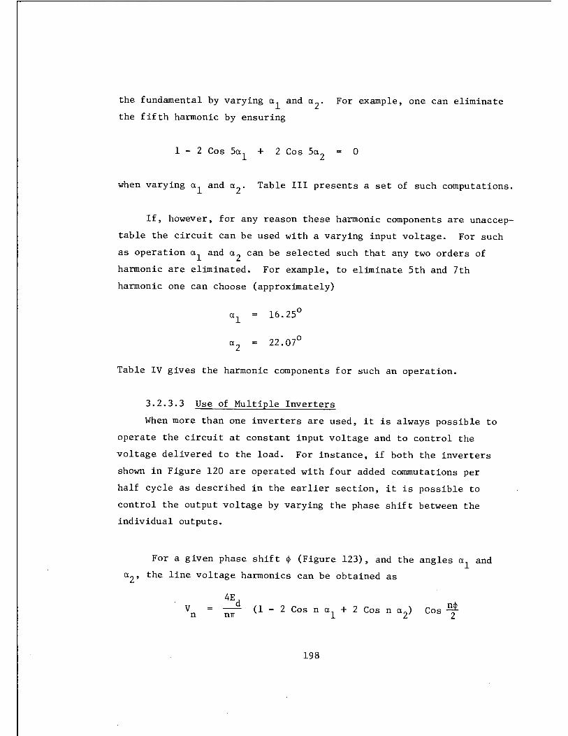
the fundamental by varying a 1 and a 2 . For example, one can eliminate
the fifth harmonic by ensuring
1 - 2 Cos 5a1
+ 2 Cos 5a2
= 0
when varying a 1 and a 2 • Table III presents a set of such computations.
If, however, for any reason these harmonic components are unaccep
table the circuit can be used with a varying input voltage. For such
as operation a 1 and a 2 can be selected such that any two orders of
harmonic are eliminated. For example, to eliminate 5th and 7th
harmonic one can choose (approximately)
16.25°
22.07°
Table IV gives the harmonic components for such an operation.
3.2.3.3 Use of Multiple Inverters
When more than one inverters are used, it is always possible to
operate the circuit at constant input voltage and to control the
voltage delivered to the load. For instance, if both the inverters
shown in Figure 120 are operated with four added commutations per
half cycle as described in the earlier section, it is possible to
control the output voltage by varying the phase shift between the
individual outputs.
For a given phase shift~ (Figure 123), and the angles a1
and
a 2 , the line voltage harmonics can be obtained as
V = n n1r
198
Cos~ 2
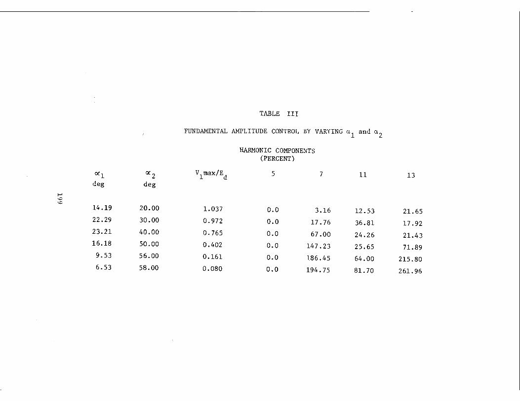
TABLE III
FUNDAMENTAL AMPLITUDE CONTROL BY VARYING a. 1 and a.2
HARMONIC COMPONENTS (PERCENT)
0(1 0( 2 V1max/Ed 5 7 11 13 deg deg
I-'
'° '° 14.19 20.00 1.037 o.o 3.16 12.53 21.65 22.29 30.00 0.972 0.0 17.76 36.81 17.92 23.21 40.00 0.765 o.o 67.00 24.26 21.43 16.18 50.00 0.402 o.o 147.23 25.65 71.89 9.53 56.00 0.161 o.o 186.45 64.00 215.80 6.53 58.00 0.080 0.0 194.75 81.70 261.96
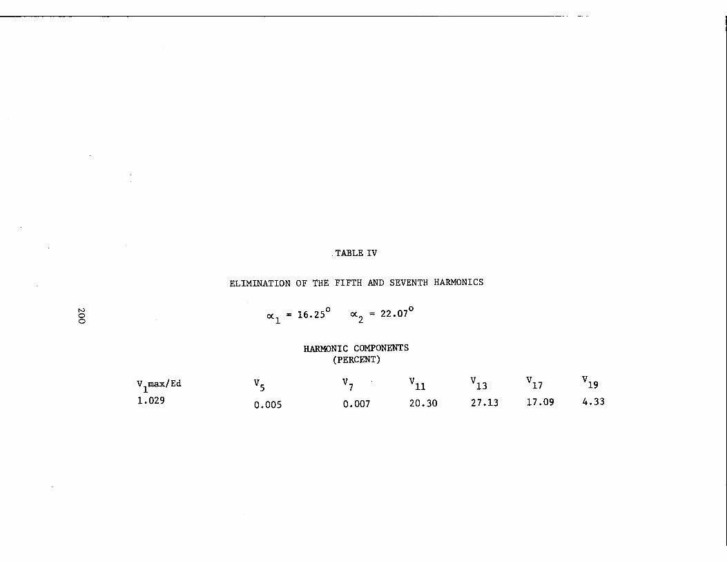
N 0 0
v1max/Ed
1.029
TABLE IV
ELIMINATION OF THE FIFTH AND SEVENTH HARMONICS
0(1 = 16.25° 0(2 = 22.07°
vs 0.005
HARMONIC COMPONENTS (PERCENT)
v7
0.007
Vll
20.30
v13
27.13
v17
17.09
Vl9
4.33

e a-0
r 00 I
e b-0 0 ~o
11
....
e a-b 0 0
I
e a-o O r 0 I
e b-O o ' 0
,--
e a-b
0 0
I
E
t /·- n r I o
180° a 2=33.3
.. ~ 0
a1
=23.62
¢=30° _l
180' - ~ ~ -
180°
... (a)
E - 2a·- n . I 180°
0 .. ...;_ a 2=33.3
I 0
a1
=23.62
¢=150° - 1r 180~ r r-..
.
l18C0
.. 1 ... .. (b) ¢=150°
FIGURE 123
E - d ..
2 00 ll 36
L....I
- -3 -.. 3 60°
- ~
~
I
Ed -2 3 -I
36 00 . ..
36 00
I
OUTPUT VOLTAGE FOR DIFFERENT PHASE DIFFERENCE
201
Again it can be seen that the angles a 1 and a 2 can be selected to
eliminate any two required orders of harmonics and V can be varied n by varying the phase shift~- In many industrial applications where
the load can be connected to the inverter through transformers, a 1 and a
2 can be selected to eliminate 5th and 7th harmonics and the
third harmonic can be avoided with proper transformer connections.
However, if the motor is directly connected to the inverter as in the
case of vehicle propulsion, a 1 and a2
should be chosen such that the
third and the fifth harmonics are eliminated, i.e.
1 - 2 Cos 3 a 1 + 2 Cos 3 a 2 = 0
1 - 2 Cos 5 a 1 + 2 Cos 5 a 2 = 0
The approximate solution of these equations is
23.62°
33.30°
The fundamental amplitude and the harmonic components for these values
of a 1 and a2
are given in Table V for different values of the phase
shift~- It should be noted that at higher values of~ when the
fundamental component is small, the harmonic components are excessive.
Another way to operate the circuit of Figure 119 is to have many
commutations per half cycle. This day it is generally possible to
eliminate all harmonics below the frequency of pulses occuring in the
output voltage. Figure 124 shows two possible operations of this
type. In Figure 124(a), a consecutive pulses have equal width and
the voltage can be controlled by simultaneously varying the width of
all pulses while maintaining the pulse frequency constant and
202

TABLE V
MULTIPLE INVERTER CONTROL WITH ELIMINATION OF THE THIRD AND FIFTH HARMONICS
HARMONIC COMPONENTS
(PERCENT)
cl> v1max
degrees Ed 3 5 7 9 11 13 15 17
N 0 1.068 0.015 0.065 29.52 48.68 36.20 3.51 19.95 16.07 0 w
30 1.032 0.011 0.017 7.91 35.60 36.20 3.51 14.60 4.31
60 0.925 o.o 0.065 29.52 o.oo 36.20 3.51 o.o 16.07
90 0.756 0.015 0.065 29.52 48.68 36.20 3.51 19.95 16.07
120 0.534 0.030 0.065 29.52 97.35 36.20 3.51 39.90 16.07
150 0.277 0.042 0.24 110.17 132.98 36.20 3.51 54.50 60.00
180 o.o o.o 0.0 0.0 0.0 o.o 0.0 o.o o.o

N 0 .i:,-
ti n n n m n n n 01800 • . . . ~ u u u 3600
ea-b 0
o I I I I I I I I LI LI LI □ -ID Li (a) PULSES OF EQUAL WIDTH
~ ~ ~ ~ m ~ ~ ~ Lao0
0° I I I I I I I I ~ ~ ~ ~ @ ~ ~ ~ ~ 36o
0
(b) PROGRAM:-tED COMMUTATION
FIGURE 124 OUTPUT VOLTAGES WITH MANY COMMUTATIONS
PER HALF CYCLE
synchronized to the output frequency. In Figure 124(b), the pulse
widths of consecutive pulses vary in sinusoidal fashion. Here the
voltage can be controlled by varying the width of all pulses while
still retaining the sinusoidal relationship and the repetition rate
of the pulses. This type of inverter is commonly known as a pulse
width-modulated i.e., a PWM inverter.
The PWM inverter is very widely used in the new generation of
rail propulsion systems using induction traction motors as described
earlier in Section 4.0.
3.3 Simplified Inverter Circuit
So far we have been discussing one type of inverter circuit which
can be operated with several commutations per half cycle of the output
voltage. Such a circuit requires auxiliary thyristors in commutation
circuit. If, however, only a six-step, 120° conduction is required, a
simple inverter circuit is possible as shown in Figure 125. The basic
operation of the inverter is very similar to that of the earlier
circuit. The commutation process is different and is explained below.
Let thyristors T1
and T2
be conducting and let the capacitor
between thyristors T1
and T3
be charged with the polarity shown in
Figure 125. Now is T3
is switched on, T1
gets reverse biased and is
turned off. The load current continues to flow via T3
and the
capacitor until the capacitor is charged in the opposite direction.
The current then flows through the diode in series with T3
into the
other line of the load. Blocking diodes are used in series with the
thyristors so that capacitors do not discharge through the load con
tinuously.
This circuit can be operated either from a current source - by
using a large reactor in series - or from a voltage source - by using
205

N 0
°'
1 3 5
D
... __
4 6 2
FIGURE 125 SIMPLIFIED INVERTER CIRCUIT
THREE PHASE LOAD
a large capacitor in parallel as shown in Figure 125. Several other
inverter circuits are possible but a discussion of all these is
clearly outside the scope of this work.
207
4.0 CYCL0C0NVERTER
It has been explained earlier that a three-phase bridge rectifier
circuit operates as a rectifier for firing angle a< 90° whereas it
works as an inverter for a> 90°. We have seen that this circuit can
provide a continuously controllable de voltage of either polarity,
although the load current can only flow in one direction. Such an
operation is a 2-quadrant operation (see Figure 126). It is possible
to obtain a 4-quadrant operation by using two such converters as
shown in Figure 127. Each converter can operate at a load voltage
of either polarity and any direction of the load current can be
obtained by using one converter at a time.
A cycloconverter is essentially a 4-quadrant converter whose
firing angle is continuously changed to produced a continuously
varying mean voltage level. By controlling the amplitude and the
frequency of firing angle variation, the amplitude and the frequency
of the output voltage can be controlled. A cycloconverter is thus
ac-to-ac converter or a frequency converter.
A cycloconverter can supply power to a load of any power factor -
leading or lagging. However, since each converter can carry a current
only in one direction, the positive half cycle of the load current
must be carried by the P-converter and the negative half cycle must
be carried by the N-converter. Each converter will, of course,
operate as a rectifier or an inverter as dictated by the load voltage.
This is shown in Figure 128.
It should be noted here that the load voltage and the load
current waveforms shown in Figure 128 represent the fundamental com
ponents of highly non-sinusoidal waveforms. The ideal waveform of
an unfiltered output voltage is shown in Figure 129. It can be seen
that the firing angle a of the circuit is a function of time and
208

3 r/, Source
I
Inverter Rectifier
-V V
FIGURE 126 TWO QUADRANT OPERATION
P-Converter N-Converter
* I
___,.p
I
Inverter Rectifier
* ....,_ I ...._ ___ ........ n
P-Converter
----+----lf-----+---lrB-- V
Rectifier Inverter N-Converter
FIGURE 127 FOUR QUADRANT OPERATION
209
3 r/, Source
:

RECT.
IDLE
I', I I ' I '~ I I'---1 I I I I I
INV IDLE
RECT.
FIGURE 128 CYCLOCONVERTER OPERATION
210
Load Current
p-converter
INV n-converter

N I-' I-'
(a) Unfiltered output voltage ---Wanted component
Output current
FIGURE 129 CYCLOCONVERTER WAVEFORMS
varies almost between 0° and 180°. It should also be remembered
that these waveforms will be different if a finite connnutation
period is considered.
So far we have considered circuits where only one converter -
P or N - is conducting at a time while the other is blocked. Such
an operation is called a 'circulating current free' mode of opera
tion. For some applications, however, a cycloconverter is operated
such that both converters are operating at the same time. They are
then controlled such that the firing angles ap and aN always add to
180°, i.e., ap + aN = 180°. With such an operation, the instanta
neous output voltages of the two converters are unequal, and hence
a center-tapped reactor is introduced in the circuit (Figure 127)
to limit the circulating current.
It is possible to build three phase cycloconverter circuits
from the basic single phase circuit discussed above. One such
circuit is shown in Figure 130. The thyristors are triggered such
that at any instant of time, two thyristor groups such as say 1 and
2, feed current into the load. Out of the six thyristors in two
groups, only two thyristors conduct at a time (ideal connnutation)
depending on the instantaneous line voltages. For large power appli
cations, however, a full wave circuit shown in Figure 131 with 36
thyristors is used.
212

A
B
C
A
B
C
4
FIGURE 130 THREEPHASECYCLOCONVERTER
213
2
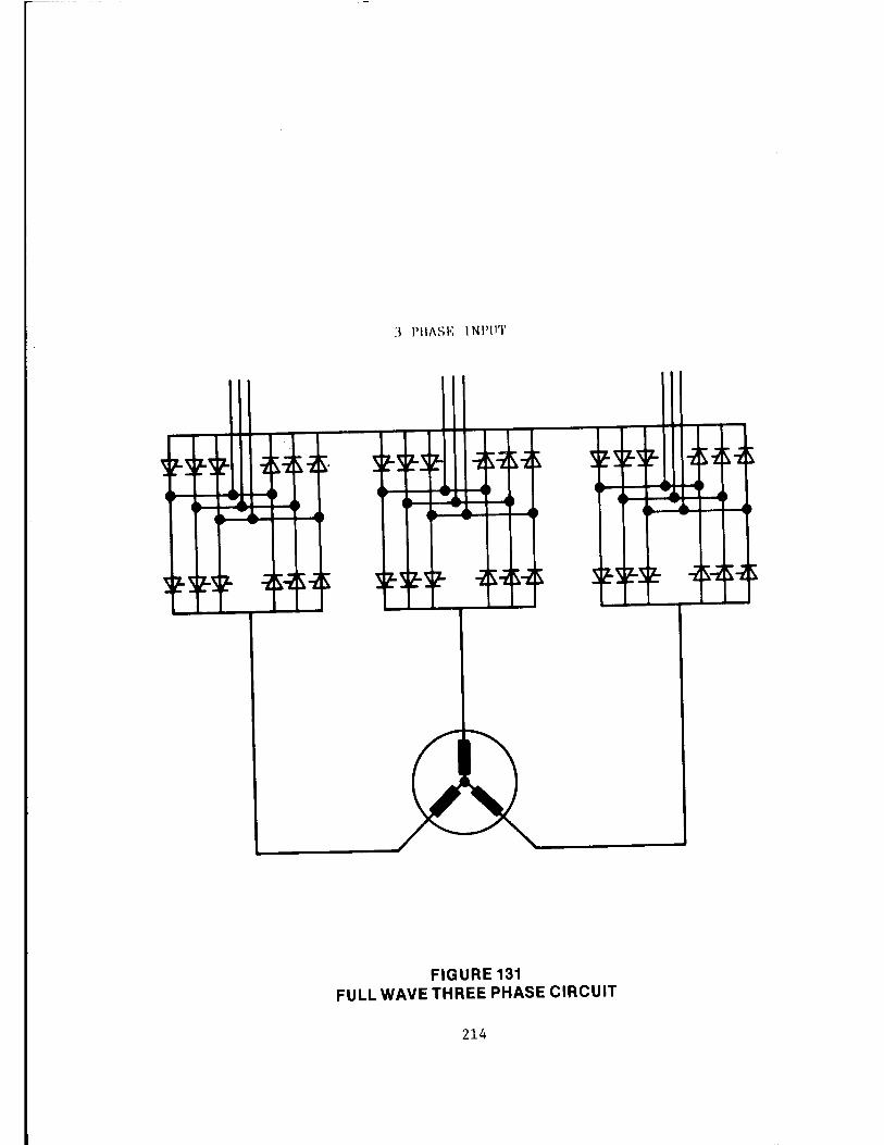
J 1'11/\SE INP\IT
FIGURE 131 FULL WAVE THREE PHASE CIRCUIT
214


![49th NCAA Wrestling Tournament 1979 3/8/1979 to … 1979.pdf49th NCAA Wrestling Tournament 1979 3/8/1979 to 3/10/1979 at Iowa State ... C.D. Mock [6] - North Carolina ... Don Finnegan,](https://img.pdfslide.us/doc/110x75/5b1e17367f8b9a397f8bb260/49th-ncaa-wrestling-tournament-1979-381979-to-1979pdf49th-ncaa-wrestling-tournament.jpg)