INTRODUCTION

Most flows occurring in nature and in engineering applications are turbulent. The boundary layer in the earth’s atmosphere is turbulent (except possibly in very stable conditions); jet streams in the upper troposphere are turbulent; cumulus clouds are in turbulent motion. The water currents below the surface of the oceans are turbulent,; the Gulf Stream is a turbulent wall-jet kind of flow. The photosphere of the sun and the photospheres of similar stars are in turbulent motion; interstellar gas clouds (gaseous nebulae) are turbulent; the wake of the earth in the solar wind is presumably a turbulent wake. Boundary layers growing on aircraft wings are turbulent. Most combustion processes involve turbulence and often even depend on it; the flow of natural gas and oil in pipelines is turbulent. Chemical engineers use turbulence to mix and homogenize fluid mixtures and to accelerate chemical reaction rates in liquids or gases. The flow of water in rivers and canals is turbulent; the wakes of ships, cars, submarines, and aircraft are in turbulent motion. The study of turbulence clearly is an interdisciplinary activity, which has a very wide range of applications. In fluid dynamics laminar flow is the exception, not the rule: one must have small dimensions and high viscosities to encounter laminar flow. The flow of lubricating oil in a bearing is a typical example.

Many turbulent flows can be observed easily; watching cumulus clouds or the plume of a smokestack is not time wasted for a student of turbulence. In the classroom, some of the films produced by the National Committee for Fluid Dynamics Films (for example, Stewart, 1969) may be used to advantage.

1 .I The nature of turbulence Everyone who, at one time or another, has observed the efflux from a smoke stack has some idea about the nature of turbulent flow. However, it is very difficult to give a precise definition of turbulence. All one can do is l is t some of the characteristics of turbulent flows.

Irregularity One characteristic is the irregularity, or randomness, of all turbulent flows. This makes a deterministic approach to turbulence problems impossible; instead, one relies on statistical methods.

2 Introduction

Diffusivity The diffusivity of turbulence, which causes rapid mixing and increased rates of momentum, heat, and mass transfer, i s another important feature of al l turbulent flows. I f a flow pattern looks random but does not exhibit spreading of velocity fluctuations through the surrounding fluid, it is surely not turbulent. The contrails of a jet aircraft are a case in point: exclud- 'ling the turbulent region just behind the aircraft, the contrails have a very nearly constant diameter for several miles. Such a flow i s not turbulent, even though it was turbulent when it was generated. The diffusivity of turbulence is the single most important feature as far as applications are concerned: it prevents boundary-layer separation on airfoils a t large (but not too large) angles of attack, it increases heat transfer rates in machinery of all kinds, it is the source of the resistance of flow in pipelines, and it increases momentum transfer between winds and Ocean currents.

Large Reynolds numbers Turbulent flows always occur a t high Reynolds numbers. Turbulence often originates as an instability of laminar flows if the Reynolds number becomes too large. The instabilities are related to the inter- action of viscous terms and nonlinear inertia terms in the equations of mo- tion. This interaction is very complex: the mathematics of nonlinear partial differential equations has not been developed to a point where general solu- tions can be given. Randomness and nonlinearity combine to make the equa- tions of turbulence nearly intractable; turbulence theory suffers from the absence of sufficiently powerful mathematical methods. This lack of tools makes all theoretical approaches to problems in turbulence trial-and-error affairs. Nonlinear concepts and mathematical tools have to be developed along the way; one cannot rely on the equations alone to obtain answers to problems. This situation makes turbulence research both frustrating and challenging: it is one of the principal unsolved problems in physics today.

Three-dimensional vorticity fluctuations Turbulence is rotational and three dimensional. Turbulence is characterized by high levels of fluctuating vor- ticity. For this reason, vorticity dynamics plays an essential role in the des- cription of turbulent flows. The random vorticity fluctuations that char- acterize turbulence could not maintain themselves if the velocity fluctuations were two dimensional, since an important vorticity-maintenance mechanism known as vortex stretching is absent in two-dimensional flow. Flows that are substantially two dimensional, such as the cyclones in the atmosphere which

3 1 .I The nature of turbulence

determine the weather, are not turbulence themselves, even though their char- acteristics may be influenced strongly by small-scale turbulence (generated somewhere by shear or buoyancy), which interacts with the large-scale flow. In summary, turbulent flows always exhibit high levels of fluctuating vor-, ticity. For example, random waves on the surface of oceans are not in turbu- lent motion since they are essentially irrotational.

Dissipation Turbulent flows are always dissipative. Viscous shear stresses perform deformation work which increases the internal energy of the fluid a t the expense of kinetic energy of the turbulence. Turbulence needs a continu- ous supply of energy to make up for these viscous losses. I f no energy is supplied, turbulence decays rapidly. Random motions, such as gravity waves in planetary atmospheres and random sound waves (acoustic noise), have insignificant viscous losses and, therefore, are not turbulent. In other words, the major distinction between random waves and turbulence is that waves are essentially nondissipative (though they often are dispersive), while turbulence is essentially dissipative.

Continuum Turbulence is a continuum phenomenon, governed by the equa- tions of fluid mechanics. Even the smallest scales occurring in a turbulent flow are ordinarily far larger than any molecular length scale. We return to this point in Section 1.5.

Turbulent flows are flows Turbulence is not a feature of fluids but of fluid flows. Most of the dynamics of turbulence is the same in all fluids, whether they are liquids or gases, i f the Reynolds number of the turbulence is large enough; the major characteristics of turbulent flows are not controlled by the molecular properties of the fluid in which the turbulence occurs. Since the equations of motion are nonlinear, each individual flow pattern has certain unique characteristics that are associated with i t s initial and boundary condi- tions. No general solution to the Navier-Stokes equations is known; conse- quently, no general solutions to problems in turbulent flow are available. Since every flow is different, it follows that every turbulent flow i s different, wen though all turbulent flows have many characteristics in common. Students of turbulence, of course, disregard the uniqueness of any particular turbulent flow and concentrate on the discovery and formulation of laws that describe entire classes or families of turbulent flows.

4 Introduction

- The characteristics of turbulence depend on i t s environment. Because of

this, turbulence theory does not attempt to deal with all kinds and types of flows in a general way. Instead, theoreticians concentrate on families of flows with fairly simple boundary conditions, like boundary layers, jets, and wakes.

1.2 Methods of analysis Turbulent flows have been investigated for more than a century, but, as was remarked earlier, no general approach to the solution of problems in turbu- lence exists. The equations of motion have been analyzed in great detail, but it is st i l l next to impossible to make accurate quantitative predictions without relying heavily on empirical data. Statistical studies of the equations of motion always lead to a situation in which there are more unknowns than equations. This is called the closure problem of turbulence theory: one has to make (very often ad hoc) assumptions to make the number of equations equal to the number of unknowns. Efforts to construct viable formal pertur- bation schemes have not been very successful so far. The success of attempts to solve problems in turbulence depends strongly on the inspiration involved in making the crucial assumption.

This book has been designed to get this point across. In turbulence, the equations do not give the entire story. One must be willing to use (and capable of using) simple physical concepts based on experience to bridge the gap between the equations and actual flows. We do not want to imply that the equations are of l i t t le use; we merely want to make it unmistakably clear that turbulence needs spirited inventors just as badly as dedicated analysts. We recognize that this i s a very specific, and possibly biased, point of view. It is possible that a t some time in the future, someone will succeed in developing a completely formal theory of turbulence. However, we believe that there is a far better chance of developing a physical model of turbulence in the spirit of the Rutherford model of the atom. The model need not be complete, but it would be very useful. The real challenge, it seems to us, is that no adequate model of turbulence exists today.

Turbulence theory is limited in the same way that general fluid dynamics would be i f the Stokes relation between stress and rate of strain in Newtonian fluids were unknown. This illustration is not arbitrary: one approach to tur- bulence theory is to postulate a relation between stress and rate of strain that involves a turbulence-generated "viscosity," which then supposedly plays a

5 1.2 Methods of analysis

role similar to that of molecular viscosity in laminar flows. This approach is based on a superficial resemblance between the way molecular motions trans- fer momentum and heat and the way in which turbulent velocity fluctuations transfer these quantities. Phenomenological concepts like "eddy viscosity" (to replace molecular viscosity) and "mixing length" (in analogy with the mean free path in the kinetic theory of gases) were developed by Taylor, Prandtl, and others. These coqcepts are studied in detail in Chapter 2.

Molecular viscosity is a property of fluids; turbulence is a characteristic of flows. Therefore, the use of an eddy viscosity to represent the effects of turbulence on a flow is liable to be misleading. However, current research seems to indicate that, in simple flows, we may, for analytical reasons, speak of a turbulent fluid rather than of a turbulent flow. Turbulent "fluids," however, are non-Newtonian: they exhibit viscoelasticity and suffer memory effects. In favorable circumstances, the memory is fading in time, so that one may be able to develop a semilocal theory relating the mean stress to the mean rate of strain.

Phenomenological theories of turbulence make crucial assumptions a t a fairly early stage in the analysis. In recent years, a group of theoreticians (Kraichnan, Edwards, Orszag, Meecham, and others) have developed very formal and sophisticated statistical theories of turbulence, in the hope of finding a formalism that does not need ad hoc assumptions (see Orszag, 1971). So far, however, rather arbitrary postulates are needed in these theories, too. The mathematical complexity of this work is so overwhelming that a discussion of i t has to be le f t out of this book.

Dimensional analysis One of the most powerful tools in the study of turbu- lent flows is dimensional analysis. In many circumstances it is possible to argue that some aspect of the structure of turbulence depends only on a few independent variables or parameters. If such a situation prevails, dimensional methods often dictate the relation between the dependent and independent variables, which results in a solution that is known except for a numerical coefficient. The outstanding example of this is the form of the spectrum of turbulent kinetic energy in what is called the "inertial subrange."

Asymptotic invariance Another frequently used approach is to exploit some of the asymptotic properties of turbulent flows. Turbulent flows are char- acterized by very high Reynolds numbers; it seems reasonable to require that

6 Introduction

any proposed descriptions of turbulence should behave properly in the limit as the Reynolds number approaches infinity. This is often a very powerful con- straint, which makes fairly specific results possible. The development of the theory of turbulent boundary layers (Chapter 5) is a case in point. The limit process involved in an asymptotic approach is related to vanishingly small effects of the molecular viscosity. Turbulent flows tend to be almost indepen- dent of the viscosity (with the exception of the very smallest scales of mo- tion); the asymptotic behavior leads to such concepts as "Reynolds-number similarity" (asymptotic invariance).

Local invariance Associated with, but distinct from, asymptotic invariance is the concept of "self-preservation" or local invariance. In simple flow geom- etries, the characteristics of the turbulent motion a t some point in time and space appear to be controlled mainly by the immediate environment. The time and length scales of the flow may vary slowly downstream, but, if the turbulence time scales are small enough to permit adjustment to the gradually changing environment, it is often possible to assume that the turbulence is dynamically similar everywhere if nondimensionalized with local length and time scales. For example, the turbulence intensity in a wake is of order 6 aU/ay, where 6 is the local width of the wake and W / a y is the average mean-velocity gradient across the wake.

Because turbulence consists of fairly large fluctuations governed by non- linear equations, one may expect a behavior like that exhibited by simple nonlinear systems with limit cycles. Such behavior should be largely indepen- dent of initial conditions; the characteristics of the limit cycle should depend only on the dynamics of the system and the constraints imposed on it. In the same way, one expects that the structure of turbulence in a given class of shear flows might be in some state of dynamical equilibrium in which local inputs of energy should approximately balance local losses. If the energy transfer mechanisms in turbulence are sufficiently rapid, so tha't effects of past events do not dominate the dynamics, one may expect that this limit- cycle type of equilibrium is governed mainly by local parameters such as scale lengths and times. Simple dimensional methods and similarity arguments can be very useful in this kind of situation. Because one may want to look for local scaling laws (both in the spatial and the spectral domain), the problem of finding appropriate length and time scales becomes an important one. Indeed, scaling laws are a t the heart of turbulence research.

7 1.3 The origin of turbulence

1.3 The origin of turbulence In flows which are originally laminar, turbulence arises from instabilities at large Reynolds numbers. Laminar pipe flow becomes turbulent at a Reynolds number (based on mean velocity and diameter) in the neighborhood of 2,000 unless great care is taken to avoid creating small disturbances that might trigger transition from laminar to turbulent flow. Boundary layers in zero pressure gradient become unstable a t a Reynolds number U6"lv = 600 approximately (6" i s the displacement thickness, U is the free-stream velo- city, and v i s the kinematic viscosity). Free shear flows, such as the flow in a mixing layer, become unstable a t very low Reynolds numbers because of an inviscid instability mechanism that does not operate in boundary-layer and pipe flow. Early stages of transition can easily be seen in the smoke rising from a cigarette.

On the other hand, turbulence cannot maintain itself but depends on its environment to obtain energy. A common source of energy for turbulent velocity fluctuations is shear in the mean flow; other sources, such as buoy- ancy, exist too. Turbulent flows are generally shear flows. If turbulence arrives in an environment where there is no shear or other maintenance mech- anism, it decays: the Reynolds number decreases and the flow tends to become laminar again. The classic example is turbulence produced by a grid in uniform flow in a wind tunnel.

Another way to make a turbulent flow laminar or to prevent a laminar flow from becoming turbulent is to provide for a mechanism that consumes turbulent kinetic energy. This situation prevails in turbulent flows with imposed magnetic fields a t low magnetic Reynolds numbers and in atmos- pheric flows with a stable density stratification, to cite two examples.

Mathematically, the details of transition from laminar to turbulent flow are rather poorly understood. Much of the theory of instabilities in laminar flows is linearized theory, valid for very small disturbances; it cannot deal with the large fluctuation levels in turbulent flow. On the other hand, almost all of the theory of turbulent flow is asymptotic theory, fairly accurate at very high Reynolds numbers but inaccurate and incomplete for Reynolds numbers a t which the turbulence cannot maintain itself. A noteworthy excep- tion is the theory of the late stage of decay of wind-tunnel turbulence (Batchelor, 1953).

Experiments have shown that transition is commonly initiated by a pri-

8 Introduction

mary instability mechanism, which in simple cases is two dimensional. The primary instability produces secondary motions, which are generally three dimensional and become unstable themselves. A sequence of this nature gen erates intense localized three-dimensional disturbances (turbulent "spots"), which arise a t random positions a t random times. These spots grow rapidly and merge with each other when they become large and numerous to form a field of developed turbulent flow. In other cases, turbulence originates from an instability that causes vortices which subsequently become unstable. Many wake flows become turbulent in this way.

1.4 Diffusivity of turbulence The outstanding characteristic of turbulent motion is i ts ability to transport or mix momentum, kinetic energy, and contaminants such as heat, particles, and moisture. The rates of transfer and mixing are several orders of magni- tude greater than the rates due to molecular diffusion: the heat transfer and combustion rates of turbulent combustion in an incinerator are orders of magnitude larger than the corresponding rates in the laminar flame of a candle.

Diffusion in a problem with an imposed length scale Contrasting laminar and turbulent diffusion rates is a useful exercise not only for getting acquainted with turbulence but also for recognizing the multifaceted role of the Rey- nolds number. Suppose one has a room (with a characteristic linear dimension L ) in which a heating element (radiator) is installed. If there is no air motion in the room, heat has to be distributed by molecular diffusion. This process is governed by the diffusion equation (8 is the temperature; 7 is the thermal diffusivity, assumed to be constant):

(1.4.1)

We are not looking for a specific solution of (1.4.1) with a given set of boundary conditions. Instead, we want to discover the gross consequences of (1.4.1) with the simple tools of dimensional analysis. Dimensionally, (1.4.1) may be interpreted as

A8 A8 - - r p ' Trn

(1.4.2)

9 1.4 Diffusivity of turbulence

where A6 is a characteristic temperature difference. From (1.4.21, we obtain

LZ T,- - ,

Y (1.4.3)

which relates the time scale T,,, of the molecular diffusion to the independent parameters L and y. If the characteristic linear dimension L (the length scale) of the room is 5 m, the time scale T, of this diffusion process is of the order of lo6 sec (more than 100 h). In this estimate the value of y for air at room temperature and pressure has been used (y = 0.20 cm2/sec). We conclude that molecular diffusion is rather ineffective in distributing heat through a room.

On the other hand, even fairly weak motions, such as those generated by small density differences (buoyancy), can disperse heat through the room quickly. Suppose that the turbulent motion of the air in the room may also be characterized by the length scale L (that is, motions are present of scales < L). This is a fair assumption, since large-scale motions are most effective in distributing heat and since the largest possible scales of motion can be no larger than the size of the room. We also need a characteristic velocity u (this u may be thought of as an rms amplitude of the velocity fluctuations in the room). For flow with a length scale L and a velocity scale u, the characteristic time is

L Tt--.

U (1.4.4)

Apparently, Tt can be determined only if u can be estimated. Suppose the radiator heats the air in i t s vicinity by A6 degrees Kelvin. This causes a buoyant acceleration g Ae/O, which is of order 0.3 m/secz if 4 6 = 10°K. This acceleration probably occurs only near the surface of the radiator. I f it has a height h = 0.1 m, the kinetic energy of the air above the radiator is ghA6/6, which is of order 0.03 (m/sec)’ per unit mass. This corresponds to a velocity of 17 cm/sec. Much of the kinetic energy, however, is lost because of the stable vertical temperature gradient in the room (the air near the ceiling tends to be hotter than the air near the floor). A characteristic velocity u of order 5cm/sec may be a reasonable average throughout the room. With u = 5 cm/sec and L = 5 m, Tt becomes 100 sec, or about 2 min. Of course, we s t i l l have to rely on molecular diffusion to even out small-scale irregularities in the temperature distribution. However, the turbulence generates eddies as small as about 1 cm (this estimate can be obtained with simple equations

10 Introduction

based on the dissipation of kinetic energy; those are discussed in Section 1.5). The temperature gradients associated with these small eddies are smeared out by molecular diffusion in a time of ordereZ/y (see Section 7.31, which is only a few seconds if e = 1 cm.

Diffusion by random motion apparently is very rapid compared to molecular diffusion. The ratio of the turbulent time scale Tt to the molecular time scale T, is the inverse of the Peclet number:

Since for gases the heat conductivity y i s of the same order of magnitude as the kinematic viscosity v (for air vly = 0.73; this ratio is known as the Prandtl number), and since we are discussing only orders of magnitude, we may write without compromise,

(1.4.6)

In our example, the Reynolds number R i s about 15,000. This exercise shows that the Reynolds number of a turbulent flow may be

interpreted as a ratio of a turbulence time scale to a molecular time scale that would prevail in the absence of turbulence in a problem with the same length scale. This point of view is often more reliable than thinking of R as a ratio of inertia terms to viscous terms in the governing equations. The latter point of view tends to be misleading because a t high Reynolds numbers viscous and other diffusion effects tend to operate on smaller length scales than inertia effects.

Eddy diffusivity Since the equations governing turbulent flow are very complicated, it is tempting to treat the diffusive nature of turbulence by means of a properly chosen effective diffusivity. In doing so, the idea of trying to understand the turbulence itself is partly discarded. If we use an effective diffusivity, we tend to treat turbulence as a property of a fluid rather than as a property of a flow. Conceptually, this is a very dangerous approach. However, it often makes the mathematics a good deal easier.

If the effects of turbulence could be represented by a simple, constant scalar diffusivity, one should be able to write for the diffusion of heat by turbulent motions,

11 1.4 Diffusivity of turbulence

ae az8 a t aX,ax, - = K - (1.4.7)

in which K is the representative diffusivity (often called "eddy" diffusivity but sometimes called the "exchange coefficient" for heat). In order to make this equation a t least a crude representation of reality, one must insist that the value of K be chosen such that the time scale of the hypothetical turbulent diffusion process is equal to that of the actual mixing process. The time scale associated with (1.4.7) is roughly

LZ T - -

K ' (1.4.8)

and the actual time scale is Tt, given by (1.4.4). Equating T with Tt, one finds

K-UL. (1.4.9)

It should be noted that this is a dimensional estimate, which cannot predict the numerical values of coefficients that may be needed. Expressions like (1.4.91, with experimentally determined coefficients, are used frequently in practical applications.

The eddy diffusivity (or viscosity) K may be compared with the kinematic viscosity Y and the thermal conductivity 7:

(1.4.1 0)

One concludes that this particular Reynolds number may also be interpreted as a ratio of apparent (or turbulent) viscosity to molecular viscosity. A note of warning is in order, though. In most flow problems, many different length scales exist, so that the interpretation of Reynolds numbers based on these length scales may not always be as straightfotward as in the example used here.

It cannot be stressed too strongly that the eddy diffusivity K is an artifice which may or may not represent the effects of turbulence faithfully. We investigate this question carefully in Chapter 2.

Diffusion in a problem with an imposed time scale As another example of the diffusivity of turbulence, we look a t boundary layers in the atmosphere. The boundary layer in the atmosphere i s exposed to the rotation of the earth.

12 Introduction

In a rotating frame of reference, flows are accelerated by the Coriolis force, which is twice the vector product of the flow velocity and the rotation rate. I f the angular velocity of the frame of reference is f/2, it follows that atmos- pheric flows have an imposed time scale of orderllf. At a latitude of 40 degrees, the value of f for a Cartesian coordinate system whose z axis is parallel to the local vertical is about sec-' (f is called the Coriolis parameter).

If the boundary layer in the atmosphere were laminar, it would be governed by a diffusion equation like (1.4.1), so that i t s length and time scales would be related by

L k - vT. (1.4.1 1)

With v = 0.15 cm2 sec-' and T = f-' = lo4 sec, this gives L, = 40 cm. In reality, however, the atmospheric boundary layer is nearly always

turbulent; a typical thickness is about lo3 m (1 km). One can obtain some appreciation for this by replacing v by K in (1.4.11) and substituting for K with (1.4.9). This yields

Lt - uT, (1.4.1 2)

which, of course, merely rephrases (1.4.4). In turbulent boundary-layer flows, the characteristic velocity of the turbulence is typically about 30 of the mean wind speed. For a wind speed of 10 m/sec, we thus estimate that u - 0.3 m/sec. With T = l / f = lo4 sec, (1.4.12) then yields L, - 3 x lo3 m (3 km), which is indeed of the same order as the observed thickness.

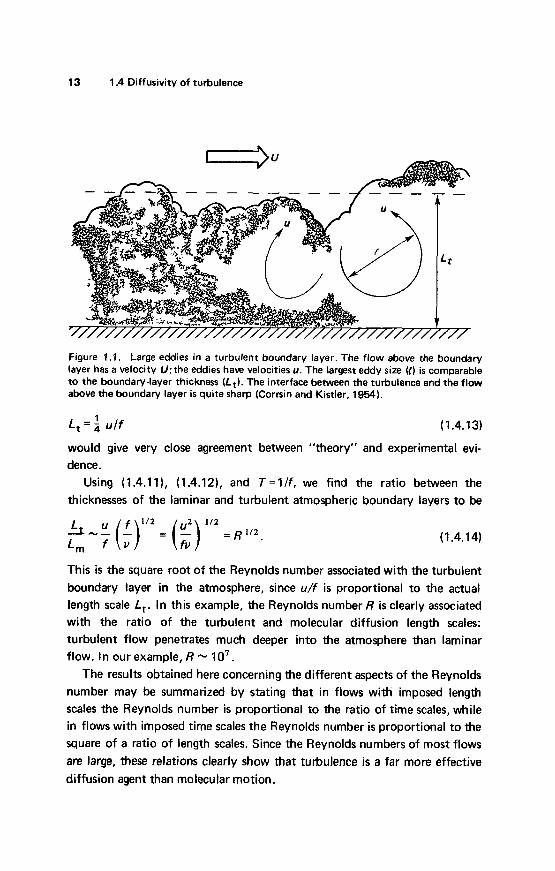
From a somewhat different point of view, we may argue that turbulent eddies with a characteristic velocity u, exposed to a Coriolis acceleration which imposes a time scale l/f, must have a size (length scale) of order u/f. It should be noted that we can equate eddy size and boundary-layer thickness only because in most turbulent flows the larger eddies seem to have sizes comparable to the characteristic size of the flow in a direction normal to the mean flow field (Figure 1.1). In estimates of diffusion or mixing, the large eddies are relevant because they perform most of the mixing (K - ueincreases with eddy size).

Arguments of this nature are often supplemented by experiments to determine the numerical coefficient in formulas like (1.4.12), because this coefficient cannot be found by dimensional reasoning. In the case of the atmospheric boundary layer,

1

13 1.4 Diffusivity of turbulence

Figure 1.1. Large eddies in a turbulent boundary layer. The flow above the boundary layer has a velocity U ; the eddies have velocities u. The largest eddy size ( l ) is comparable to the boundary-layer thickness (Lt). The interface between the turbulence and the flow above the boundary layer is quite sharp (Corrsin and Kistler, 1954).

L t =1 4 ulf (1.4.13)

would give very close agreement between ”theory” and experimental evi- dence.

Using (1.4.111, (1.4.12), and T = l / f , we find the ratio between the thicknesses of the laminar and turbulent atmospheric boundary layers to be

(1.4.14)

This is the square root of the Reynolds number associated with the turbulent boundary layer in the atmosphere, since u/f is proportional to the actual length scale L,. In this example, the Reynolds number R is clearly associated with the ratio of the turbulent and molecular diffusion length scales: turbulent flow penetrates much deeper into the atmosphere than laminar flow. In our example, R - lo’.

The results obtained here concerning the different aspects of the Reynolds number may be summarized by stating that in flows with imposed length scales the Reynolds number is proportional to the ratio of time scales, while in flows with imposed time scales the Reynolds number is proportional to the square of a ratio of length scales. Since the Reynolds numbers of most flows are large, these relations clearly show that turbulence is a far more effective diffusion agent than molecular motion.

14 Introduction

The examples discussed here are rather crude because only a single length or time scale has been taken into account. Most turbulent flows are far more complicated; this introduction would not be complete without a look a t turbulence as a multiple lengthscale problem.

1.5 Length scales in turbulent flows The fluid dynamics of flows a t high Reynolds numbers is characterized by the existence of several length scales, some of which assume very specific roles in the description and analysis of flows. In turbulent flows a wide range of length scales exists, bounded from above by the dimensions of the flow field and bounded from below by the diffusive action of molecular viscosity. Incidentally, this is the reason why spectral analysis of turbulent motion is useful.

Laminar boundary layers Let us take a look a t the problem of multiple scales in laminar shear flows. For steady flow of an incompressible fluid with constant viscosity, the Navier-Stokes equations are

(1.5.1)

One would be tempted to estimate the inertia terms as Uz/L (U being a characteristic velocity and L a characteristic length) and to estimate the viscous terms as vU/L2. The ratio of these terms is UL/v = R, indicating that viscous terms should become negligible a t large Reynolds numbers. However, boundary conditions or initial conditions may make it impossible to neglect viscous terms everywhere in the flow field. For example, a boundary layer has to exist in the flow along a solid surface to satisfy the no-slip condition. This can be understood by allowing for the possibility that viscous effects may be associated with small length scales. The viscous terms can survive a t high Reynolds numbers only by choosing a new length scale tsuch that the viscous terms are of the same order of magnitude as the inertia terms. Formally,

U2/L -vu/P. ( 1.5.2)

The viscous length t i s thus related to the scale L of the flow field as

(1.5.3)

15 1.5 Length scales in turbulent flows

The viscous length G i s a transverse length scale: it represents the width (thickness) of the boundary layer, because it relates to the molecular diffusion of momentum deficit across the flow, away from the surface. Molecular diffusion along the flow, of course, is negligible compared to the downstream transport of momentum by the flow itself. Figure 1.2 illustrates this situation.

Diffusive and convective length scales As (1.5.3) indicates, the boundary- layer thickness may be considerably smaller than the scale L of the flow field in which the boundary layer (or other laminar shear flow) develops. The distinction between a "diffusive" length scale across the flow and a "convective" length scale along the flow is essential to the understanding of all shear flows, both laminar and turbulent. Many shear flows are very slender: their width is much smaller than their "length" (that is, the distance from some suitably defined origin). The wide separation between lateral and longitudinal length scales in shear flows leads to very attractive simplifying approximations in the equations of motion; without this feature, analysis would be next to impossible.

The most powerful of the asymptotic approximations associated with d/L + 0 is that the shear flow becomes independent of most of i ts environ- ment, except for the boundary conditions imposed by the overall flow. The use of words like boundary layers, wakes, fronts in weather systems, jetstreams, and the Gulf Stream is not a semantic accident. Because of the wide difference in length scales, these shear flows are identifiable as distinct regions in flow fields. These regions have distinct dynamics and distinct

Figure 1.2. Length scales, diffusion, and convection in a laminar boundary layer over a flat plate.

16 introduction

characteristics; they are governed by specific equations of motion, which, in the asymptotic approximation &'L+ 0, may be substantially simpler than the equations governing other parts of the flow field.

Turbulent boundary layers It is useful to compare turbulent shear flows to laminar ones, even though we can do so a t t h i s moment only in a very rudimentary way. The relevant length and velocity scales in a turbulent boundary layer are illustrated in Figure 1.3. The turbulent eddies transfer momentum deficit away from the surface. With characteristic velocity fluctuations of order u, the boundary-layer thickness L' presumably increases roughly as &/dt - u (see Section 5.5). The time interval elapsed between the origin of the boundary layer and the downstream position L is of order L/U (convective time scale), so that we may estimate L'- ut - uL/U. In effect, we are equating the turbulent "diffusion" time scale t/u to the convective time scale L/U. This procedure could also have been used for laminar boundary layers. In laminar boundary layers, the diffusion distance L' increases as (vt) 1'2 ;with t = L/U, the result (1.5.2,1.5.3) i s retrieved.

In analogy to (1.4.4) and (1.4.1 2), we thus can write the scale relations for turbulent boundary layers as

t / L - u/u, (1.5.4)

e/u .-, L/U. (1.5.5)

\\\\\\\\\\\\\\\\\\\\\\\\\\\\\\\\\\\\\\'

Figure 1.3. Length and velocity scales in a turbulent boundary layer. The time passed since the fluid at L passed the origin of the boundary layer is of order L/U.

17 1.5 Length scales in turbulent flows

These relations merely relate characteristic lengths and velocities; they should not be used as formulas to compute the rate of spreading of a turbulent boundary layer. The relation between the time scales, (1.5.51, rephrases the fundamental assumption we implicitly encountered earlier, that is, that in a situation with an imposed external flow the turbulence, being part of the flow, must have a time scale commensurate with the time scale of the flow. As we will see later, this assumption conflicts with eddy-viscosity concepts. Fortunately, not all of the turbulence has such a large time scale: the small eddies in turbulence have very short time scales, which tend to make them statistically independent of the mean flow.

Laminar and turbulent friction If we compare (1.5.3) and (1.5.4) and introduce experimental data, which suggest that u/U is of the order of lo-' over a wide range of Reynolds numbers, we again get some appreciation for the relatively rapid growth of turbulent shear flows. This rapid growth should correspond to a larger drag coefficient.

For a steady laminar boundary layer in twodimensional flow on a plate with length L, the drag D per unit span is equal to the total rate of loss of momentum. Estimating the momentum loss as pU2e, where 8 is a boundary- layer thickness a t the end of the plate, we may put

D - pU 2t. (1.5.6)

The drag coefficient (or friction coefficient) Cd is defined by

(1.5.7)

Substituting (1.5.6) into (1.5.7) and using the relation for t /L given by (1.5.3), we obtain

(1.5.8)

For a turbulent boundary layer, on the other hand, the mass flow deficit a t the end of the plate is proportional to pul (see Chapter 51, so that the rate of loss of momentum is proportional to (pu4U. Consequently,

e cd N 2 - = 2R-112. L

D - puUC (1.5.9)

18 Introduction

The drag coefficient then becomes, if we use the definition (1.5.7) and the scale relation (1.5.4),

( 1.5.1 0)

Experimental evidence shows that the turbulence level u/U varies very slowly with Reynolds number, so that the drag coefficient of a turbulent boundary layer, given by (1.5.101, should be very much greater than the drag coefficient of a laminar boundary layer (1.5.8). Figure 1.4 illustrates this point. Similar conclusions are valid for heat- and mass-transfer coefficients.

Equation (1.5.4) has another interesting implication. In boundary layers and wakes u/U and t /L tend to zero as L increases beyond limit. In jets entering fluid a t rest and shear layers, on the other hand,u/U andL‘/L approach finite asymptotic values as L +m. This distinction is the origin of some important differences in the asymptotic treatment of the two different types of flow. In particular, jets and mixing layers spread linearly, while wakes and boundary layers grow slower the farther downstream they travel. Even so, most turbulent shear flows spread slowly enough to make& + 0 a useful approximation.

19 1.5 Length scales in turbulent flows

Small scales in turbulence So far only the largest eddy sizes in turbulent flows have been considered, because the large eddies do most of the transport of momentum and contaminants. We have suggested that large eddies are as big as the width of the flow and that the latter is the relevant length scale in the analysis of the interaction of the turbulence with the mean flow. For some of the other aspects of the dynamics of turbulence, however, other length scales are needed.

We shall attempt to find the smallest length scales in turbulent flows. At very small length scales, viscosity can be effective in smoothing out velocity fluctuations. The generation of small-scale fluctuations is due to the nonlinear terms in the equations of motion; the viscous terms prevent the generation of infinitely small scales of motion by dissipating small-scale energy into heat. This is characteristic of a small parameter like Y (more properly 1/R) with a singular behavior. One might expect that a t large Reynolds numbers the relative magnitude of viscosity is so small that viscous effects in a flow tend to become vanishingly small. The nonlinear terms in the Navier-Stokes equation counteract this threat by generating motion a t scales small enough to be affected by viscosity. The smallest scale of motion automatically adjusts itself to the value of the viscosity. There seems to be no way of doing away with viscosity: as soon as the scale of the flow field becomes so large that viscosity effects could conceivably be neglected, the flow creates small-scale motion, thus keeping viscosity effects (in particular dissipation rates) a t a finite level.

Since small-scale motions tend to have small time scales, one may assume that these motions are statistically independent of the relatively slow large-scale turbulence and of the mean flow. If this assumption makes sense, the small-scale motion should depend only on the rate a t which it is supplied with energy by the large-scale motion and on the kinematic viscosity. It is fair to assume that the rate of energy supply should be equal to the rate of dissipation, because the net rate of change of small-scale energy is related to the time scale of the flow as a whole. The net rate of change, therefore, should be small compared to the rate a t which energy is dissipated. This is the basis for what is called Kolmogorov's universal equilibrium theory of the small-scale structure (Chapter 8).

This discussion suggests that the parameters governing the small-scale motion include a t least the dissipation rate per unit mass E (m2 S ~ C - ~ ) and the

20 Introduction

kinematic viscosity v (mZ sec-' 1. With these parameters, one can form length, time, and velocity scales as follows:

(1.5.1 1)

These scales are referred to as the Kolmogorov microscales of length, time, and velocity (see Friedlander and Topper, 1962). In the Russian literature, these scales are called "inner" scales.

The Reynolds number formed with q and u i s equal to one

qulv = 1, (1.5.12)

which illustrates tha t the small-scale motion is qu i te viscous and tha t the viscous dissipation adjusts itself to the energy supply by adjusting length scales.

An inviscid estimate for the dissipation rate One can form an impression of the differences between the large-scale and small-scale aspects of turbulence if the dissipation rate e can be related to the length and velocity scales of the large-scale turbulence. A plausible assumption is to take the rateatwhich large eddies supply energy to small eddies to be proport ional to the reciprocal of the t ime scale of the large eddies. The amoun t of kinetic energy per unit mass in the large-scale turbulence is proport ional to u 2 ; the rate of transfer of energy is assumed to be proport ional to u/t: where [represents the size of the largest eddies or the width of the flow. We shall see later t ha t [relates to the "integral" scales of turbulence, which can be measured by statistical methods. To avoid confusion, we identi fy d' f r o m here on as the "integral scale," leaving a more precise def in i t ion for Chapter 2. Russian scientists speak of "outer" scales rather than of integral scales.

The rate of energy supply to the small-scale eddies is thus of order u2 *u/t= u3/L This energy is dissipated a t a rate e, which should be equal to the supply rate. Hence (Taylor, 1935),

e - u ~ e , (1.5.13)

which states that viscous dissipation of energy can be estimated from the large-scale dynamics, which do not involve viscosity. In this sense, dissipation again is clearly seen as a passive process in the sense tha t it proceeds a t a rate dictated by the inviscid inertial behavior of the large eddies.

The estimate (1.5.13) should not be passed over l ightly. It is one of the

21 1.5 Length scales in turbulent flows

Figure 1.5. Sketch of the nonlinear breakdown of a drop of ink in water.

cornerstone assumptions of turbulence theory; it claims that large eddies lose a significant fraction of their kinetic energy uz within one "turnover" time t/u. This implies that the nonlinear mechanism that makes small eddies out of larger ones is as "dissipative" as i t s characteristic time permits. In other words, turbulence is a strongly damped nonlinear stochastic system. Some re- searchers believe that this feature may be related to the entropy production concept embodied in the second law of thermodynamics. It should be kept in mind, however, that large eddies lose a negligible fraction of their energy to direct viscous dissipation effects. The time scale of their decay is d2 /v , so that their viscous energy loss proceeds a t a rate vu2/d2 , which is small compared to 0 3 / t i f the Reynolds number udv i s large. The nonlinear mechanism is dissipative because it creates smaller and smaller eddies until the eddy sizes become so small that viscous dissipation of their kinetic energy is almost immediate. The reader may gain some appreciation for the vigor of this process by observing drops o (Figure 1.5).

Scale relations Substituting

qlt- (~elv)-~'~ = R-3'4.

rule- r / t = (u&)-'" = R-' '2,

VIU - ( u ~ v ) - " ~ = R-'I4.

ink or mill

1.5.13) into

that are put in a glass of water

1.5.1 I), we obtain

( 1.5.1 4)

(1.5.15)

(1.5.1 6)

These relations indicate that the length, time, and velocity scales of the

22 Introduction

smallest eddies are very much smaller than those of the largest eddies. The separation in scales widens as the Reynolds number increases, so tha t one may suspect that the statistical independence and the dynamical equilibrium state of the small-scale structure of turbulence will be most evident at very large Reynolds numbers.

The main difference between two turbulent flows with different Reynolds numbers but with the same integral scale is the size of the smallest eddies: a turbulent flow at a relatively low Reynolds number has a relatively "coarse" small-scale structure (Figure 1.6). Visual evidence of the small-scale structure can be obtained if temperature fluctuations are present in the turbulence. Temperature and index of refraction gradients are steepest if they are associated with the smallest eddies; any optical system tha t is sensitive to such fluctuating gradients "sees" the small-scale structure of turbulence. The trembling, jittery horizon seen on a very hot day and the random pattern of

Figure 1.6. Turbulent jets a t different Reynolds numben: (a) relatively low Reynolds number, (b) relatively high Reynolds number (adapted from a film sequence by R . W. Stewart, 1969). The shading pattern used closely resembles the small-scale structure of turbulence seen in shadowgraph pictures.

23 1.5 Length scales in turbulent flows

light and dark seen on the wall next to a heating element in sunlight are good illustrations.

Vorticity has the dimensions of a frequency (sec-' 1. The vorticity of the small-scale eddies should be proportional to the reciprocal of the time scale 7. From (1.5.1 5) we conclude that the vorticity of the small-scale eddies is very much larger than that of the large-scale motion. On the other hand, (1.5.16) indicates that the small-scale energy is small compared to the large-scale energy. This is typical of all turbulence: most of the energy is associated with large-scale motions, most of the vorticity is associated with small-scale motions.

Molecular and turbulent scales The Kolmogorov length and time scales are the smallest scales occurring in turbulent motion. At this point, it is convenient to demonstrate that most turbulent flows are indeed continuum phenomena. The Kolmogorov scales of length and time decrease with increasing dissipation rates. High dissipation rates are associated with large values of u. In gases, large values of u are more likely to occur than in liquids. Therefore, it is sufficient to show that in gases the smallest turbulent scales of motion are normally very much larger than molecular scales of motion. The relevant molecular length scale is the mean free path t . The velocity scale of molecular motion in a gas is proportional to the speed of sound a in the gas. Kinetic theory of gases shows that the product a5 is proportional to the kinematic viscosity of the gas:

v - at. (1.5.17)

The ratio of the mean free path t to the Kolmogorov length scale q (this might be called a microstructure Knudsen number) becomes (Corrsin, 1959)

t lq - M/R 'I4, (1.5.18)

where we have used (1.5.14) and (1.5.17). In (1.5.18) the turbulence Reynolds number R = UQV and the turbulence Mach number M = u/a are used as independent variables. It is seen that turbulence might interfere with molecular motion a t high Mach numbers and low Reynolds numbers. This kind of situation is unlikely to occur, because M is seldom large, but R is typically very large. A pertinent illustration i s the situation in gaseous nebulae (cosmic gas clouds) (Spitzer, 1968). In clouds that consist mainly of neutral

24 introduction

hydrogen, the turbulent Mach number is of order 10 (u - 10 km/sec, a - 1 km/sec), while the Reynolds number is of order l o7 (1- 10l7 m, $! - 10' ' m). With (1.5.181, we compute that g/q - 1/6. In this extreme case, it seems doubtful that the smallest eddies perceive a continuum. In clouds that consist mainly of ionized hydrogen, temperatures are quite high, increasing a to about 10 km/sec and decreasing M to about 1. The mean free path .$ remains roughly the same (the density in ionized clouds is not appreciably different from that in neutral clouds), so that R reduces to about lo6 . In this case, [/q-&, which may be small enough for the smallest eddies to operate in a continuum.

The ratio of the time scale r to the collision time scale [/a associated with molecular motion is, in terms of R and M,

ra/g- R ' I 2 MP2. (1.5.19)

For M = 10 and R = lo', the smallest time scale of turbulence is 32 times as large as the collision time scale of the gas molecules; for M = 1 and R = lo6 the ratio is 1000. It should be recognized that in ionized gases other length and time scales are associated with the motion of the microscopic particles and with the several other dynamical processes (radiation, cosmic rays, magnetic fields) that may be present, so that r ) may not always be a relevant length scale.

Because the smallest time scales in turbulent motion tend to be much larger than molecular. time scales, the motion of the gas molecules is in approximate statistical equilibrium, so that molecular transport effects may indeed be represented by transport coefficients such as viscosity and heat conductivity. These representations would become invalid if the departures from equilibrium were large; the case t / q - g , ra/[ - 32 would probably re- quire treatment with the methods of statistical mechanics.

1

1.6 Outline of the material The bird's-eye view of turbulence dynamics given in the preceding sectioris sets the stage for a brief outline of this book. In Chapter 2, we deal with eddy-viscosity and mixing-length theories. The dimensional framework of these theories is useful in the analysis of typical shear flows. In Chapter 3, the energy and vorticity equations of turbulent flow are derived. In Chapter 4, some free shear flows like wakes and jets are discussed. In Chapter 5,

25 Problems

boundary layers are analyzed. To prepare a formal basis for the study of diffusion and spectral dynamics, an introduction to statistics is given in Chapter 6. In Chapter 7, turbulent diffusion and mixing are studied.

The study of the spatial dynamics of turbulent flows precedes that of the spectral dynamics. There exist many similarities and analogies between spatial and spectral dynamics of turbulence. Also, spatial dynamics can be visualized more easily by those new to the subject. Once some of the subtle features of turbulent shear flow are understood, the dynamics of turbulence in wave- number space should not be too perplexing. Spectral dynamics is studied in Chapter 8.

Problems

1.1 Estimate the energy dissipation rate in a cumulus cloud, both per unit mass and for the entirecloud. Base your estimates on velocity and length scales typical of cumulus clouds. Compute the total dissipation rate in kilowatts. Also estimate the Kolmogorov microscale 7. Use p = 1.25 kg/m3 and Y = 15 x m2/sec.

1.2 A cubical box of volume L 3 is filled with fluid in turbulent motion. No source of energy is present, so that the turbulence decays. Because the turbulence is confined to the box, i ts length scale may be assumed to be equal to L a t all times. Derive an expression for the decay of the kinetic energy ?u2 as a function of time. As the turbulence decays, i t s Reynolds number 2 decreases. If the Reynolds number uL/v becomes smaller than 10, say, the inviscid estimate f = u3/L should be replaced by an estimate of the type f = cvu2/L2, because the weak eddies remaining at low Reynolds numbers lose their energy directly to viscous dissipation. Computec by requiring that the dissipation rate i s continuous a t uL/v = 10. Derive an expression tor the decay of the kinetic energy when uL/u < 10 (this is called the "final" period of decay). I f L = 1 m, v = 15 x m2 /sec and u = 1 m/sec a t time t = 0, how long does it take before the turbulence enters the final period of decay? Assume that the effects of the walls of the box on the decay of the turbu- lence may be ignored. Can you support this assumption in any way?

1.3 The large eddies in a turbulent flow have a length scalet, a velocity scale v(fl = u, and a time scale to =&I. The smallest eddies have a length

26 introduction

scale 9, a velocity scale u, and a time scale 7. Estimate the characteristic velocity v( r ) and the characteristic time t (r) of eddies of size r , where r is any length in the range r )<r< t . Do t h i s by assuming that v(r) and t(r) are determined by E and r only. Show that your results agree with the known velocity and time scales a t r =t and r = r). The energy spectrum of turbulence is a plot of E ( K ) = K-' v2 ( K ) , where K = l / r i s the "wave number" associated with eddies of size r . Find an expression for E ( K ) and compare your result with the data in Chapter 8.

1.4 An airplane with a hot-wire anemometer mounted on its wing tip is to fly through the turbulent boundary layer of the atmosphere a t a speed of 50 m/sec. The velocity fluctuations in the atmosphere are of order 0.5 m/sec, the length scale of the large eddies i s about 100 m. The hot-wire anemometer is to be designed so that it will register the motion of the smallest eddies. What is the highest frequency the anemometer will encounter? What should the length of the hot-wire sensor be? If the noise in the electronic circuitry is expressed in terms of equivalent turbulence intensity, what is the permissible noise level?