Embed Size (px)
Citation preview

: i
,'" .. '
If you have issues viewing or accessing this file, please contact us at NCJRS.gov.
o.-====,.. ___ , ______ w -_..,....., _____ .,_l ____ ' __ -.r",.,.. ___ ~ N. - __ ==0_1"! .. .AIIr'N,......~
LOUIE L v/ A I N H R r G H T SEC RET A R Y
t .. ---·...,.===------... ------_ .. ________ ' ... · _r:t'.~a:c:au== )'«"'~ .... ,.-....." .. M,e "1IR\'WO .... ~
COMPARATIVE ANALYSIS OF POPULATION PROJECTION METHODS
Document #77-R-064
lp'1;");, 1;" P ~ In. O£1L- U] 'JI n ~ ; 1."1) 0' D u..1L ~ '-'- u Jr f.. C!. 1 1.1l. Jl..il Jl. b ,
Researcl~ arrld Statistics
• __ ... -<-4 _ .. _ .. ___ ... _-.-- ..... _.--.... ---- .. ---•• --~ ..... ---.. ' .. ~- .. -~- ....
I
----;;:-'-;--"-:-.--;:-:-;---------;-;-;-.. -.~,~~-~~-~--~~-------
... "
FLORIDA DEPARTMENT OF OFFENDER REHABILITATION LOUIE L. NAlm'lRIG1I1', SECRE'l'J\RY
.- CO~1PARATIVE ANALYSIS OF POPULATION PROJECTION METHODS
.0' .'.
'. ...~ .... , ....
SEPTEMBER 27, 1977
Robert Roesch, Bureau Chief Lonnie Fouty, Administrator of Research Robert Morgen, Intern
I ._
~~~~ ... ~~~ ~~~~. --.. ~-~. ~~----~--------~--~~------~--------~
/ /<
/
(',"
, TABLE OF CONTENTS
I. Percentage of In~rease and Liner Regression
II. IThe SIH110DG Model
Page 1
10
III. 'rhe SPACE Model . -14
IV. Survey of Methodology in Other States 16
V. Reasons for Development of the New Hodel 19
VI. Design of Sirnula ted Losses/Admissions l-1odel: Prediction of Re~eases 23
VII. Design of th~ Model: Prediction of Admissions 30 •
VIII .. Summary ..... 32
. -
-. ._ .
-.. ~ '. . _ ...
. ... --~.

1 "
P~RCENTAGE OF INCR~ASE AN~ LINEAR REGReSSION
-Effective and efficient correctional planning depends
to ~ great extent on the ability to accur~tely predict the
future irunate population. In response to this need the
Department of Offender Rehabilitation has spent consider
able tim~ in attempting to develop more satisfactory pro-
jection techniques.
For several years prior ,to 1~73, the Department used
the simple technique of projecting the past percentage of
change to estimate future population. The assumption under .. .. .
this method was that the population would change by the same
percentage in the future as it had done in the recent past.
Thus, if the inmate popul'ation had grown by 4 % over the past
year,. the projected growth rate for the future would also be
4%. In this technique, only twd data'points are used in mak-
ing projections.
In 1973, the Department began to utilize the technique
of linear regression, because of its promise of greater
accuracy. In the application of this technique by the
Department, the past values for the inmate population (the
total number of inMates at the end of each month) arc used to
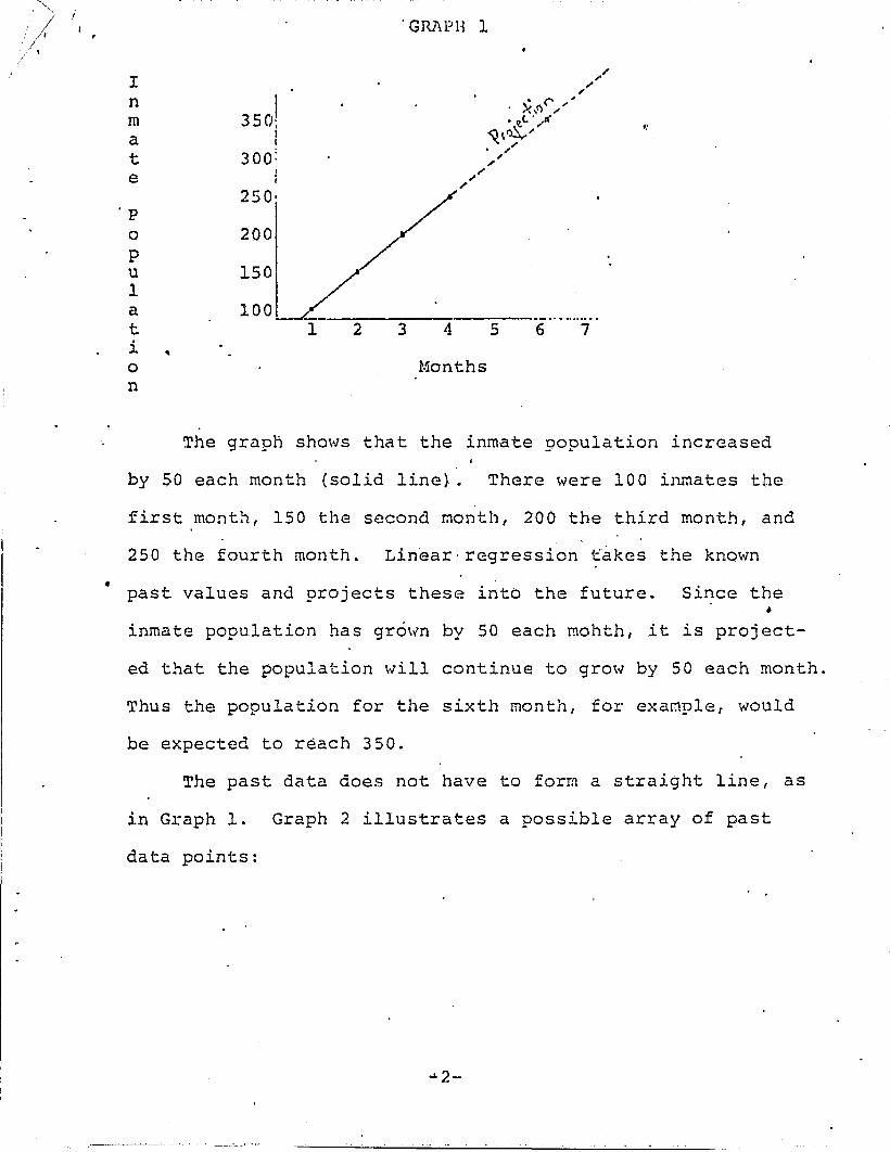
predict the future values. Graph 1 illustratas the operation
of this technique.
-1-
'( ---.--;;<--.-,.-",.-;--:--;,----;;--;-;--
/ /'
/ "
'GRAPH 1
I n m f~
a t e
p 0
p u 1 a ----------._ .......... . t 1 23456 7 i , 0 l-1onths n
The grc:tph shows that the inmate !?opulation increased
by 50 each month (solid line). There \Vere 100 inmates the
first month, 150 the second month, 200 the third month, and
250 the fourth month. Linear· regression takes the known
• past values and projects these into the future. Since the •
inmate population has grciwn by 50 each mohth, it is project-
ed that the population will continue to grow by 50 each month.
Thus the population for the sixth month, for example, would
be expected to reach 350.
The past data does not have to form a straight line, as
in Graph 1. Graph 2 illustrates a possible array of past
data points:
.J.2-
I
I .
I I
Inmate
Population
400'
3501
I 300'
I 25°1
I 200'
1501
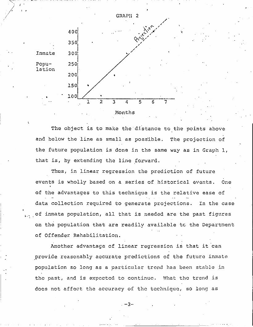
GRAPH 2
. 100 '-"'----:------------------.. -5 6 7
110nths
The object is to make the·di~tance to the points above
and below the line as small as poss'ible. The proj ection of
the future population is done in the same way as in Graph 1,
that is, by extending the line forward.
Thus r in linear reg~ession the prediction of future
events is wholly based on a series of historical events. One
of the advantages to this technique is the relative ease of
data collection required to generate projections. In the case
~,~ of inmate population, all that is needed are the past figures
on the population that are readily available te. the Depart~ent
of Offender Rehabilitation.
Another advantage of linear regression is that it 'can
.provide reasonably accurate predictions of the future inmate
population so long as a particular trend has been stable in
the past, and is e::-:pected to continue. Nhat the trend is
does not affect the Clccuracy of the tec.l1n:i.que, so long as
. -3-

/
it is a stable and linear onG. For example, there may be a .
continuous steady increase in the'inmate populntion, or a r
continuous gradual decline. ThG primary assumption of the
linear regr~ssion technique is that whatever has happened
in the pa.st !lill c:ontinue to happen :i.n the future.
Obviously, ~eal systems do not necessarily perform in
linear fashion. There are ~imes when the inmate population
fluctuat~s widely just as there are times when a stable
pattern shif~ abruptly. Under these conditions linear re-
gression is much less useful and may in fact be highly mis
leading. This is the results of limitations of the linear
regression technique in responding to major changes in critical
variables.
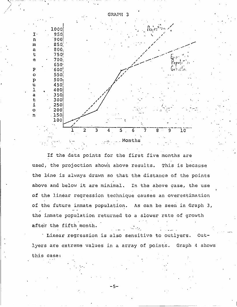
Graph 3 illustrates a situation in which linear regression
will not produce an accurate estimate. In this case there has
been a slow pattern of growth for the first three months,
folldwed by a sudden shift to a very rapid rate of growth.
-4-
,< /
/.
,---:;:-"-.-:-.-----c::-;;-;- ,
'- .
GRAPH 3
I· 10001 .. 95°1
n 900; rn 850; ZL 800·
I
t 750 t I
e 700: 650:
p . 600 1
0 5501 p 500
1 u 450 1 400 a 350 t 30°1 . '. ' . i 25°1 0 200·
I , -: '., '!t' ••
• w •• ,... :' . n . 150
100
2 3 4
. Months
If the data points for the first five months are
used, the projection show~ above results. This is because
the l'.ine is always drm·m so that the distance of the points
above and below it are minimal. In the above 9ase, the use
of the lin~ar regression technique causes an overestimation
of the future inmate populatio~. As can be seen in Graph 3,
the inmate population returned to a slower rate of growth
afte'r the fifth month. .. ... "~-
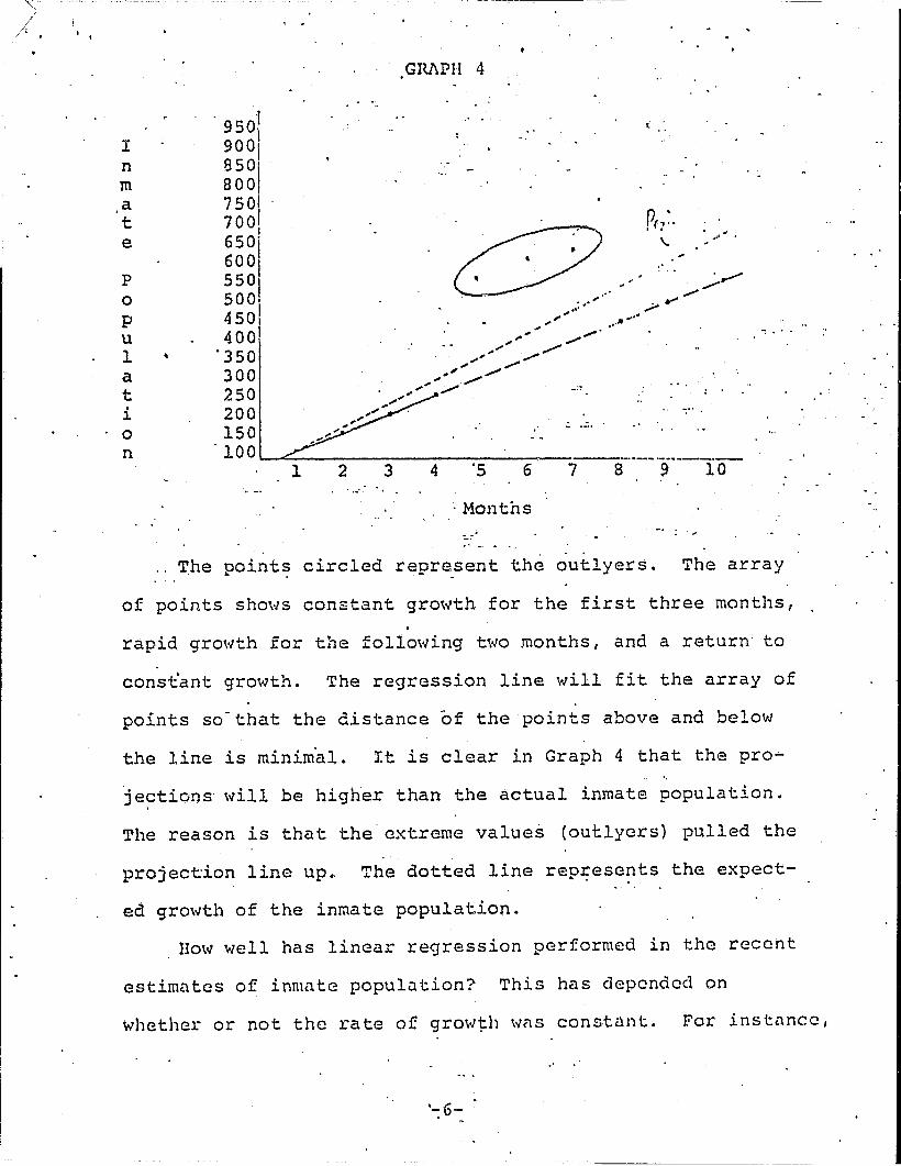
- Linear regression is also sensitive to outlyers. Out-
lyers are extreme values in a array of pointz. Graph 4 shows
this case:
.....
.'" :
-5-
.........
I
~'
/ /1 ,
I n m a t e
p 0 p u 1 a t i 0 n
,GRAPH 4
, 950' 900\ 850' 8001
r,' .',
7501 7001
I 650' 600 1
5501
5001
4501
"
.. . . ' #fII*''''»'
4001 "350 300 250 200 150 "
' 100 1 2 3 4 '5 6 7
.' _. . . ._'
. Months
-. . ' ..... , .
The point~ circled r~present the outlyers.
"
, .~ ,
The array
of points shows constant growth for the first three months, . rapid growth for the following two months, and a return' to
constant growth. The regression line will fit the array of
points so-that the distance of the points above and below
the line is minim~l. It is clear in Graph 4 that the pro
je?tions' will be higher than the actual inmate population.
The reason is that the' extreme value~ (outlycrs) pulled the
projection line up. The dotted line reoresents the expect-... ,
ed growth of the inmate population.
liow well has linear regression performed in the recent
estimntes of inmnte popul~tion? This has depended on
whether or not the rate of growth \vClS constnnt. For instnncc,
I I
i ,
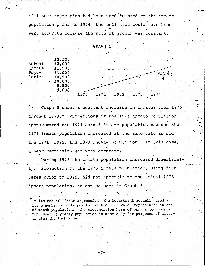
• if linear regression had been used to ~rcdict the inmate
population prior to 1974, the estimates would have been . .. . ..
. very accurate becau~e the rate Of growth was constant.
I l2,SOGi 12,OOOl
.' ~ . ...... .. .-
GRl\PH 5
, ;
_ .... -: • :....."'. - t • ,'. cd ,- ... "
....... ... Actual Inmate Population
11, 5001 11,00°1 10 150°1 10,000,
...... p' J • .. ~-.. _' _....... (,,!'~'I).' , ., I . :- • \!, .
, .... ~ .. - .. ,
9,500\ 9,000; ~"
1970 1971 1972 1973 1974
Graph s'showia constant increase in inm~tes. from 1970
through 1973.* Projections of the '1974 inmate population . ,
appro~imated the 1974 actual inmate population because the
1974 inmate population increased at the same rate as did
the 1971, 1972, and 1973 ,inmate population. In this case,
linear regression was very accurate. . .
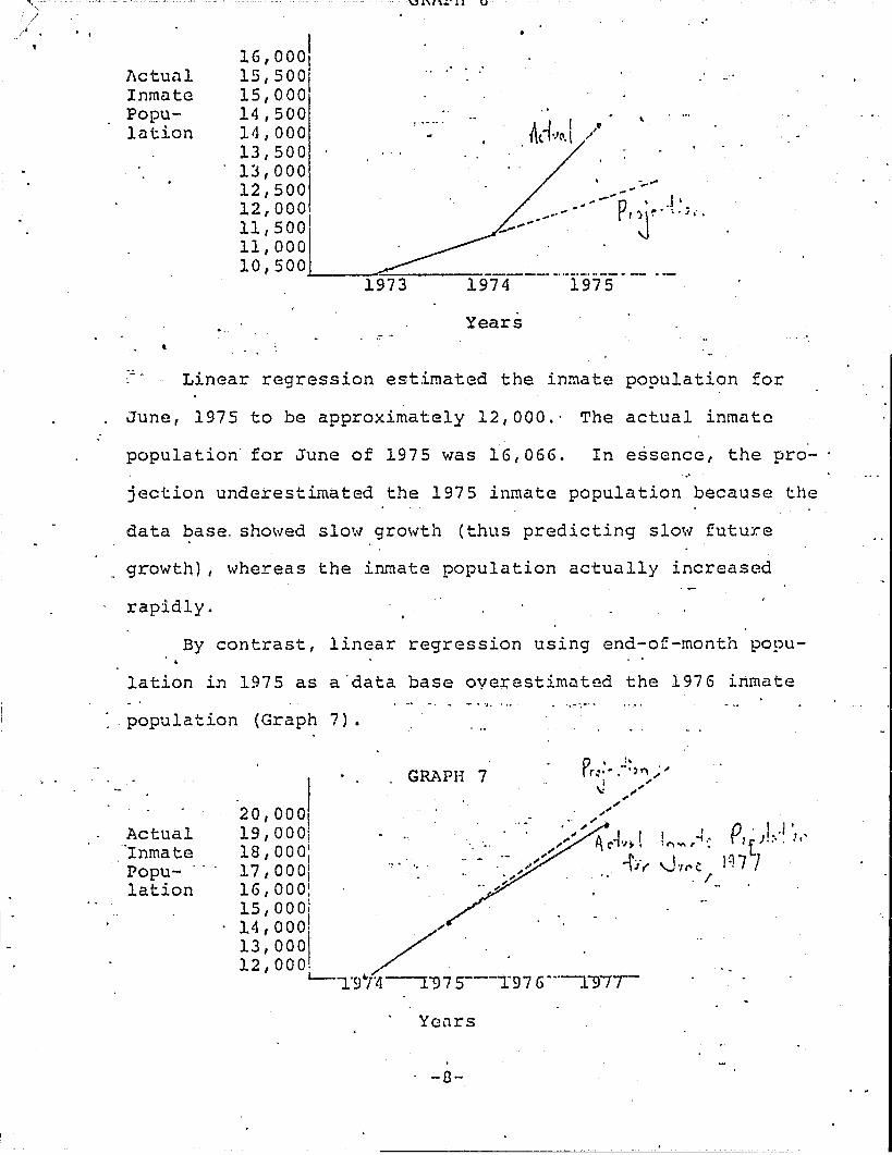
During 1975 the inmate population increased dramatical-"
ly. Projection of the 1975 inmate population, using data
bases prior to 1975, did not approximate the actual 1975
inmate population, as can be seen in Graph 6. .... ' ......... .
. " . .: ..
*1n its use of linear 'regression, t~e Department actu~il~ ~sed a large number of data points, each one of which represented an endof-month populcJ.tion. '1'he presentation here of only a few points representing yearly population is made only for purposes of illustrating the technique.
-7-
:" .'
.. '!'
.'
.., .... -
.. ". ,-
, -
}\ctu<.ll Inmate Population
,
I 16,0001 15,500' 15,0001
14,500 111,000 13,500 13,000 12,500 12,000 11,500 11,000
"
10, 5 0 O-,--_~--:-,=~ __ ~ _____ 0., __ ._. _ •• ___ ._
1974 1975
Years
.'
Linear regression estimated the inmate population for
June, 1975 to be approximately 12,000.' The actual inmate
population for June of 1975 was 16,066. In essence, the pro-
jection underestimated the 1975 inmate population because the
data base, showed slow growth (thus predicting slow future
growth), whereas the inITIate population actually increased
rapidly.
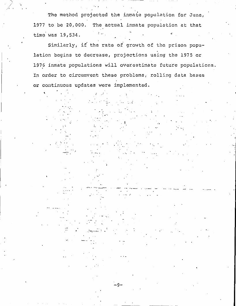
By contrast, linear regression using end-of-month popu-
lation in 1975 as a'data base overestimated the 1976 inmate - ... ~. ". . ... '~-. ~
population (Graph 7).
Actual Inmate Popu- ., , 1ation
GRAPH 7 . I 20,0001
I
19,0001
. ' .. ,.'
18,000; 17,00°1 16,OOO~ 15,000; 14,000! " ,',' . 13,0001 /'" , , . 12,00Q, /
1...-'1.·9"f'4--r"97 S---T97 6°"-r97,
Ycnrs
-8-
'I
, I
The method projected the • inmate populntion for. June,
1977 to be 20,000. The actual inr.'la te populution at that
time was 19,534. ' - r,'
Simil<lrly, if .
the rate of grO\<lth of the prison popu-.
lation begins to decrease, projections using the 1975 or
1976 inmate populations will overestimate future popuiations.
In order to circumvent these problems, rolling data bases
or continuous updates were implemented.
" ·po .. ; -" "
.. .. .,\
, ~ ','
.. ".:
.. ' ... , :.-
"
',-- - _c ........... ..
. " .. "
"
.... : '.,
....... , ...
.. --......... '-'.
, "
-9-
, ,
II
r
THE SIM~10DG MODEr .. ,
As we have indicated, the linenr regression technique
uses historical ~vents exclusively in the prediction of
future events. In the case of inmate population, the
historical events used are the past figures for total in-
mate. population. The future inmate population is seen as
following directly from the past inmate populatio~. Fairly
representative predictions are possible when the historical •
trend has been stable, and linear in nature, but not whe~
sudden shifts occur.
The problem with using the linear regression techriique
for the prediction of the future inmate population is that
there are many volatile f~ctors which may cause major shifts
in the popul~tion level. The crime rate, for exnmple, may , .
have held steady for the period of time covered by the pro~
jection, thereby increasing user confidence i~"the outcome.
This does not mean, however, that these conditions will con-
tinue unchanged ovei an indefinite period. On the contrary, .
'the crime rate may suddenly start increasing at a rapid'pace.
Using linear reg~ession, there is no way to anticipate these
important changes.
Faced with the obvious limitations of the linear re-
gression techllique, the Department of Offender Rehabilitation
-10-
.'
, . surveyed and utilized other techniquGs in an attempt to
. - . . . improve the confidence level of predictions developed by
. .. .. the DGpartrnent.
. The SIMMODG model was developed in early 1976. Rather
.than simply examining thG past innate population, the
SIMMODG model considers the criminal ju~tice system a~ a
whole. This model examines the interrelationship of prison l
parole l probation, and arrests • .
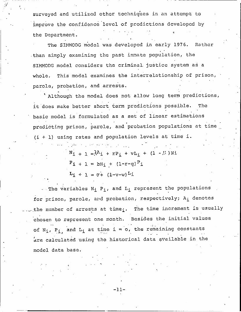
, Although the model does not allow long term predictions,
it does make better short term predictions possible. The
basic model is for~ulatcd as a set of linear estimations - ,
predi6ting prison, parole, and probation populations at time
(i + l) using rates and population levels at time i~ ~ ... . .' .... . .-
N· + I =AAi + rP' + vL' + (I - ,1.t ) N i l. l. l.
p. + 1 = bN' + (l-r-q)Pi l. l..
L· l. + 1 = 0"+ (l-V-\Ol) Li .. . The variables N' l. Pit and L· l. represent the populations
for prison, parole l a~d probation I respectively; Ai denotes
__ ._" .the number of arrests at timei' The time increment is usually
~hosen to represent one month. Besides the initial values " "
of Nil ~i, and Li at t~~e i ="0, the remaining constants I -dre calculated using the historical data available in the
model data base.
-.
-11-
,> ~~~- ---~-~~c---·~. ~-~-~~~~-~---~-----__ ~ ___________ , __ _
, '
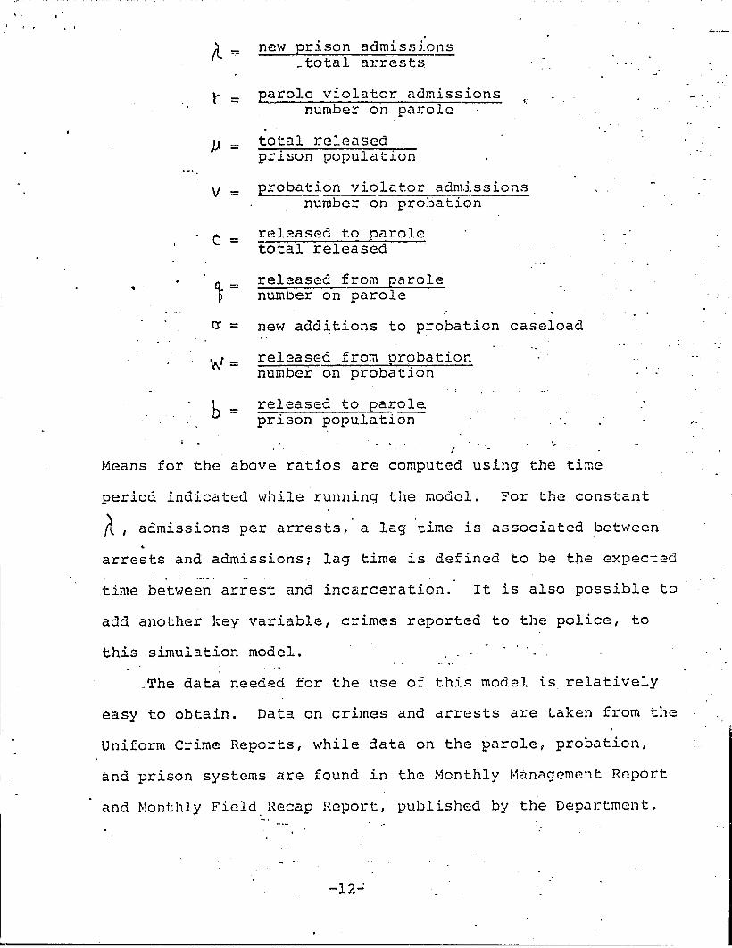
A=
t" =
)J. =
v =
. ,.. '- =
0"=
W=
b =
. new prison admissions
_total arrests
parole violator admissions number on parole
. total l:"eleascd prison population
.;
probation violator admissions number on probation
released to parole total released
released from parole number on parole
new additions to probation caseload
released from orobation number on probation
released to parole prison population
I
Means for the above ratios are computed using the time
period indicated while running the model. For the constant
(I.. , admissions per arrests,' a lag 'time is associated between
arrests and admissionsj lag time is defined to be the expected
time between arrest and incarceration. It is also possible to
add another key variable, crimes reported to the police, to
this simulation model. - .. . .
_The data needed for the use of this model is relatively
easy to obtain. Data on crimes and arrests are taken from the
uniform Crime Reports, while data on the parole, probation,
and prison systems are found in the Monthly Management Report
and Monthly Field,Recap Report, published by the Department.
-12";
· . For the. S I11t·10DG model, the pro'j actions arc vnlid for
only 6 moriths, since the primary variable is the arrcst
rate/ time lag (which at this time is estimatc~ to be six
months between arrest and cor:llni tr:1cnt). Any proj ections
exceeding 6 months are based on estimated'arrest figures,
and are thus less reliable.
The main advantage of the SI~~ODG simulation model over
the linear regression technique is that important c~anges in
the,prison population can be anticipated to some extent. The
linear regression technique discussed earlier in this paper
does not enable the Department to foresee shifts in the prison
popUlation because it assum6that past trends will continue.
With the SIMMODG model, on the other hand, the impact
of changes in the criminal justice system (especially arrest
rates) on the prison population can be gauged.
This model represen~ed an important advancement over
linear regression insofar as it used developments i~ the crimin
al justice system instead of merely relying on the end-of-month
prison population figures. Applications, however, are limited
in that projections cannot be made with confidence for an
extended time frame. When attempts were made to apply the
model, it became apparent to the Department that p~ojections
for an extended period (three years, for example) wduld depend
on making estimates of future arrest rates. This is, at
~resentt very difficult to do with any degree of confidence.
-13-
III
THE SPl\C}~ t10'DEL
Another model that wns developed for the prediction
of the inmate pop·.·.lation is the SPACE model. 'l'his model
was developed by the Council of State Governments in the
early part of 1977. Like the SIt-mODG model, SPACE attempts . , .
to si~ulate the workings of the overall criminal justic~
syste~. The purpose is to. trace the flow of offenders from
the time of their arrest to the time that they are released .. '.
from prison.
The principal purpose of the SPACE model is to predict
short-range changes in the correcti6nal population, short-
range denoting a period of not more than a year and a half.
The SPACE model can also De used to si~ulate the probable im-
pact of policy changes (such as longer sent~nces, greater
use of incarceration~ etc).
There are some significant differences between the SPACE
model and the SIMHODG model. The SPACE model uses the pro-
portion of arrests placed on, probation rather than using a
constant number of new probations. Also, this model has a time
lag built into each item that uses a rate,a feature that should
increase the accuracy of the predictions.
-14-
~. I
\ , I I
This model enables short-range predictions to be made
that turn out to be reasonably accurate. It is remarked tha t: . The Florida tes~ resul~s confir~ed the potential utility of SPACE as a valid population projection device. Using data for the period form July, 1972 until Januury, 197u,
. the program projected prison population for0ard to October, 1976, with an average margin of error of three percent.
As in the case of the SIMl'·10DG model, the SPACE model
possessed important advantages over linear regression. Once
again, however, the model~~usefulness was greatly limite~·by . . the fact ·that only short-range predictions \vere possible.
Predictions for a period of more than a year and a half are
necessary for purposes of capital improvements and budget
preparation.
As a result/ the SIlvl110DG and SPACE models were not
utilized. In 1976 the Department decided to continue using
linear regression with a moving data base while considerable
effort was made to develop improved methodologies. In the
same year, population projections were produced by applying
log transformations to the data base, and also by using a
quadratic equation with a sine curve .. The projections that
resulted from the use of these techniques indicated a huge '.. .
increase in population which appeared to the Department to
be unrealistic .. As a resul t,.· these techniques were not g i verj
further consideration. In late 1976, work'was begun on the
SIMMS model. Nork on this complex model is still in progress.
In 1977, the Department queried the other stutes on their pro-
jection methodologi.es. It also developed and began utilizing
a promising new model.
-lS-
.. • ~ I
·r'
IV
SURVEY OF l1ETHODOLOGY IN O'fnER ST1\TES ,
In its efforts to develop more sati~factory projections
of the inmate p09ulation, the Florida Dep~rtment of Offender
Rehabilitation conducted a survey of population projection
methodologies and approaches in all of the other states and
the District of Columbia. ..
Our survey shows a picture as varied as one might ex-·
pect from such a large number of diverse jurisdictions . .
Some states eschewed population projections entirely, while
others had developed rather sophisticated projection models.
In those states that hav~ done projections, and that responded
to our survey in some depth., there appears to be a general
awareness of the considerable difficulties invoived in trying
to acqurately predict the future inmate population.
One of the notable findings of the survey is the recog-
nition, in many states, that the application of linear re-
gression, using past inmate popUlation as the sole data base,
leaves a great deal to be desired. This recognition may have
come about as these states experienced the same ~udden and
unexpected surge in inmate population as occurred in Florida.
As we mentioned in Section 1 of this paper, linear regression
is of questionable value when there is a dramatic shift in a ..........
-lG-
~ 1 1 •
given pattern. This shift--to much 'higher populations-
occurred in many states between 1973 and 1975. The sudden
incrcuse in population resul ted in. crises in m~ny stu tes.
These criies invol~ed severe prison overcrowding, the use
of emergency facilities to house inmates, ~nd the effort to
quickly build-many new facilities. This situution could not ,
be anticipated using the method of linear regression. This
has led a number of states to attempt to develop more sophis
ticated methodologies.
These methodologies have often taken the form of either
mUltiple regression or simulation models. The mUltiple re
gression models are still "linear," but they utiiize more
than one factor (as the name implies}, and move away from past
inmate population levels as a predictor of future population.
The simulation models attempt to recreate the actual workings
of the criminal justice system, or part. of that system, in
order ~o gauge the impact on inmate population levels.
Several states have decided -against ,using a strict method-
ology. Instead, they have opted for a "multi-factor" approach
that takes into account a lar~e variety of factors, including
some that are difficult to quantify. In this approach a range
of estimates is frequently mad€, rather than a single es~imate.
It is apparent that there is at this time no technique
or approach that offers a "vision into the futurc" with a sure
prospect of accurate populution projections. Although much
-17-
I '
I. l'
. , valuable info~mation has been p~oduced by this survey, it is
difficult to assess the value of the competing techniques
and approaches I for two reasons .. First of all, since most "
of the promising tcchniquc~ have been developed only recently,
there has not been time to determine their us~fulness and
degree of accuracy. It may take several years to do so.
Secondly, conditions in the different states are not the same.
There are urban ~tates and rural states; states with a high
crime rate and those ~..,ith low rates; states with a high rate
of incarceration and states with a low rate of imprisonment,
and so on. A technique that is effective in one state may not .,
be effective in another state that has a different set of con-
ditions. .'
T~ble 1 shows the work that the different states have done
in the area of population projections.
.... . ......... . -. ._ I' .. '"' •• , .:" H •
··.·1 ....
; :,: ..... " .
-18-
I, I'
v
REASONS FOR DEVELOPMENT OF THe NEW MODEt
'J'hB unexDBcted qrmoJth of thB F lor ida inma te PQ~ tion
since 1973 has greatly heightened the need for more effective
forecasting tools. The inmate population, which stood at
10,669 in June,-l973: J;each~d ~9/534 by ,Inne, 1977 J an in~se
o'f 83,.1 percent in_j.u.st: fOUl: :letirs.
The very extent of this increase--in sheer numbers--makes
it essential that more accu'rate predictions be provided. The
size of the Florida system dictate requirements for facility
construction and capital outlay that are radically different
from those in a state \oJith a ~p--tisoD system. In a syste~
wi th 1, 00 a inmates. for example I afl iflerease of a 3 % !'/OU) d Ulean
the addition of 830 individuals. A similar percen~ag~ incr~ase
in Florida adced near.ly 9 1 000 inmates to the system. The re-•
quirements for additional bed spaces in the small system could
be met by the construction of one or two facilities. In a
~vstem the size of Florida's( on the other hand, an increase
of 83% in four years translates into overcrowded conditions, (
. ".
temporary erner!;d-ency housl.nq, the ne'ed for extensive construction
and huge caoital outlays. -Until recently I efforts made to predict future ininate
population levels centered around the linear regression method-
ology. As we have stated earlier in this report, the specific
I'
-19- ',' "
. ' f, I'
application of linear regression usbd by the Department
employed the moving end-of-month inmate population as the
sole data base. While utilization of this tech~ique did
not enable the Department to foresee the recent dramatic .
increase in inmute population, it also fails to show when
this increase will level off. In keeping' with the logic of
this method, it is assumed that a very l1igh rate of growth
would continue indefinitely. This is because the period .
of rapid increase was being used as the data base. It was
pla~ned that adjustments would be made to these projections , , ,
when the increase slowed, allowing the department to av6id .. :"\~.~ .
underestimation in the face of unprecedented growth.
The SIMMODG and SPACE models offered the possibility
of more reliable predictions, since they monitored develop-
ments in other parts of the criminal justice system (such as
arrest rates). The limitation of both SI~10DG and SPACE was ,....
that p~edictions could be made with confidence only for a
relatively short time period.
During the period of rapid increase in the inmate popu-
latio~ speculation centered around the question as to when
this rate of increase would level off. This spe9ulation
;.' ..
became more intense during the first six months of FY 1976-77,
as a result of a slight downturn in DOR admissions, and of re-
! . ported decreases in both crime and arrest rates.
A popular assumption was that those inmates admitted
during the period of rapid increase in FY 197A.::"·75 wOlua be
.. ' .. . . -20- "
"
. , t, It
~~~~~"'---'--~---~-"---------------""':-
released at the same rate as they had entcr:@d.-the-.I:nmate
pl"lQulation. it was. expected that the average time to be
served ,by inma tes st~IT in prison would aE.P£.oximc1 te J:he
amount of time served by inmates __ who hc1d a.1rea.9.Y-R..e-.M re-
leased from custody. It was therefore ~aLL~e~h~~.if
that over half the population admitted_in FY 1974-75 would
be released ~y the end of FY 1976-77. Honthly reports of
net qains and losses 'vere carefully scrutinized; each
month that releases exce~Qed-adm-i-s-s-~n-s-,-s.p.ec.ula tion grew
that inmate popUlation growth had, at last, leveled off . •
r,t was erroneous to assum.e..r-ho.1'Le~er, that releases -----....
would continue to exceed admissions and that the inmate
poplllat j a~'lould stabilize. Thi.s assumption resulted from
the failure to recognize the significant differences in ad
missions and releases on an_indi~Qal basis. Overall ad
missions and aggregated releases were dealt with as a
homogeneous entity, and it was therefore believed that the,
average length of tL~e served by those already released was
representative. of the time that has been and will be served
by the entire DaR population. The residual prison population
was not delineated, and its characteristics were not analyzed.
The significance of these actual characteristics of the
~mate population may be un~eratood if a hypothetical group
~f admissions and releases is examjned in a simple illus
tration. If there are 100 new admissions and 50 releases in
--a given month, the inmate population would increase in size.
"
-21-
" .
I'
- ---------~--- ~~,-----~--~~--------------
If the converse were to occur {IOO ~elcases and 50 admissions}
resulting in a net monthly loss of 50 persons, there would
be an irnmed11l~short-tcrm decrease in the size' of the..,inmate '--- --poPUla-e'±OIl. FTo\vever, if DOR released 100 persons who were
~~~~r sentences and ad~itted 50 inmates unap.r
twenty-five year sentences, the population in custody.iould
ul t'iillate-ry grO'<l over the' long rUI} q,~L, the short-term popu,lation
replaced itself ~n future months. In fact, there would have
to be1 a prolonged decline in admissions of inmates serving
relatively long sentences before a significant leveling would
occur in the growth of the inmate population, and this simply
has not happened. It is estimat'ed that it would take about
twenty-five years for the inmate population to stabilize and
reflect current moderate declines in admission without signi-
ficant changes in sentencing policy by the courts.
'.
, ' . , .
-22-
..
..
VI
DESIGN OF SD1ULATED LOSSES/l\Dt,lISSIONS MODEL: PREDICTION OF RELEl\SES
The design of the Simulated Losses/Admissions Moddl
addresses certain characteristics of the DOR inmate popu-
lation that have'not been eff~ctively considered in other ,
'foreqasts.
Historically, the growth of the'DOR inmate population
has been analyzed in terms of gross admissions and releases.
Linear projection and computation of net gains/losses treats,
each release and each admission as being statistically equal.
Prior cooparisons of numbers of admissions with nuober of
releases were appropriate for providing static head counts
but proved inadequate for ~aking long-term or even short-term
projections.
Previous inmate population forecasts did not accqunt for
the fact that the offender flow consists of a number of in-
dividual cases, each differing in length of sentence, offense,
and other demographlc and circumstantial characteristics that
de fin e th e 1 elliLth-e-:f.--t;-ime-t;.ha:t-a-n-e-:E-fende..r-w.i.J..L.ema in in .- ~
_custodJ!. ,:
Monitoring the numbers at intake and release without
determinip:J the length of time that offenders are likely to
remain in the status population makes estimation of the size
"
. . , -23-
. ' . '
I -
! •
and/or characteristics of the futuic residual population
impossibler Consideration of the characteristics of each' , ' /
offender that are significant.to the amount of , time he will
actually serve is essential to dciterming the rate o~ release
of both the residual population and the n~w admissions.
For example, t~e admission of an offender with a twenty-
year sentence cannot be accurately compared (on a one-to-one,
gross release subtracted from gr6ss admission basis) to the
releqse of a person with a three-year sentence. In terms of
the siz~ of the residual inmate population/ the admitted in-
mate replaces the released inmate for an initial three-year
period but the long-range implication over the additional
time served will not be measurable under previously used
methodologi.es.
In order to determine an indicator of the time an offend-
er would actually remain i? Drison, a number of variables
were examined. Among these were off'7nse, len<;Jth of sentence,
race I age, and prior cor.uni tment t'o DOR. The highest correla-
tion with time served (r= .66) occurred with the length of
sentence.
Once it has been established that length of sentence
co~elates most strongly with actual time served, it is
necessary to quantify the relationship so tha~ it may be
simulated. ' The greatest problem in case-by-case prediction
of release dates is that the only data available on length
'<. '. # • -24-
'.
.. I'
"
c.-~~~ .• ~~~-~~~~~~~~---~---------____ _
of time served is data dcrivad from tha records of in~atcs . \vho have already be~n released. This data has been signifi-
. ,
cantly biased as a result of the dramatic incr~ase in ad-
missions over the past four years.
As a representative sample, the automated data aase for
releases as compared to th~ unprecedented number of recent
admissions and the current status population is extremely·
limited. While ~here may be as many as 95% of the one-year
'and ~\Vo--year admissions accounted for on the release tapes
sincie FY 1974-75, the percent of releases for longer sentences
is extremely small. For instance, the number of releases re-
ported for persons sentenced to.life imprisonment was 127 over
the two year period. However, ~here are currently more than
1,650 offenders in DOR institutions serving life sentences.
Of these released, the longest time served on a life sentence
was about 19 years while some of those not released ha ...... e se'rved
more than 30 years at this time.
In order to predict release dates, we examined: 1) the
am~~n~ :ime-~erved by those already rel~ased,
2) the amount of time that has been served by those still in
prison, and 3)' the estimated amount of remaining time to be
served by those still in prison based upon the available sa~pl~
--of historical data derived from 1 and 2.
. Initially, only the average length o~ time served by
selected length-of-senten~e classes was examined. The results
of adding the average time served to each admission date for
' .. '
.:
. ~ •. . .. .'
-25- .',1 Of
-'. I .. '. . "
I'
thos~ .1.n custody, counting the numbers released over time,
and then comparing,the release pattern ovor the same period
with the actual releases, prove~ to be unacceptable. It
was determined that the 11 stundard deviation" or the UT.1ount
of variance in distribution of releases from the mean
(average) had to be considered. Release distribution curves
were thus constructed for each of the length-af-sentence
classes to be used as a basis for the simulation.
The first part of the release module was designed to
produce a series of distributions of length-of-time served
for fourteen length-of-sentence classes. These were used
to simulate the actual rate of release of inmates and to pre-
dict future releases.
There w~re just over 2,000 admissions in FY 1976-77. In
order to predict" the number of inmates among 8, 000 adr:1issions
who \vould be released after serving some. number of months
(36 months for example), the computer tapes listing offenders
released during FX 1974-75 and FY 1975-76 were examined to
determine the actual number released after 36 months.
These inmates would have been admitted during FY 1971-72 and
FY 1972-73 when admissions were about 5,000 per year. Assum-
ing the examination of this historical data indicated that 50
inmates per year had been released after 36 months, then it
would be predicted, based upon u constant proportion, that 80 . "
out of 8,000 offenders ad.~itted in FY 1976-77 \vould be released,
.. " -26-
" "
. ' after 36 months. Since 8,000 is ~.G times 5,000, each
of these SO inmates in the historical sample would have"
to be assigned a weight of 1.6 so that ~hey wdqld represent
80 inmates in the release distributions. Therefore, the
program is designed so that a weight is ~ssigned to each
release record according to the inrna~e'~ year of adrniision
as a means of adjusting for the inordinate increase in
admissions that has occurred over the last few years .
• In"addition, the length of time served for each release
record was multiplied by a varying factor for each l~ngth of
sentence class. The reason that the length of time served
had to be increased was that the unadjusted release distrib-
utions (derived from an analysi;s of time served by the set
of inmates who have been released) were not reoresentativc , .. of the time served by inmates still in the prison system.
Especially for longer ~entences, the unadjusted release dis-
tributions were based upon relatively small samples compared
with the number of inmates still in prison. Some of those
inmates not yet released have alrE~ady served terms consider-
ably longer than the sample of inmates who have been released
and upon whose records the unadjusted release distributions
are based. Adjustment of the actual release distributions
was also made to compensate for unusual levels of releases
in the parole sector. After the two adjustments were made
for each release record, the fourteen length-of-sentence
,
-27-. ' ', .. ,\~::~.,;f~, , .
' ..
"
..
, \
release distributions used in the simulation were generated
on a monthly basis.
The next part of the progrnm,works in this manner: for
the first length of sentence class, the release distribution
is called Net), where t represents the number of months to
be served and N(t) represents the number of inmates who would.
serve exactly t months. A new function r A(t), is defined as
follo~vs :
ACt} = N(l) + N(2) + + N (t) .
A(t) represents the number of inmates who would serve t months
or fewer. The inverse of A(t) is called T(n) I where n rep-
resents a nu;nbering of inmates to be released with respect "
to this distribution in the order that they would be released.
T(n} represents the number of months after which the nth in-
mate would be released. /
These functions are used in the second
part of the release module. Similar ~unctions were defined for
the other length of sentence classes.
The second part of the release module predicts monthly
releases by assigning a predicted release date tb each inmate
currently in custody or admitted to the prison system. The
June 30 1 1973, computer status tape and the admission tapes
for Fy'1973-74, FY 1974-75, and FY 1975-76 were used as the '. data base and the program predicting the releases is called
the Release Prediction Program •
. .
-2B-
For each inmate admitted to pr~son after June 30, 1973,
the adjusted release distribution N(t), along with ACt) and
Ten) is selected corresponding to the inmate's length of
sentence. A number, X, representing the inmate to be released, .
is chosen at random along the vertical axis. T(K), therefore,"
will be the predicted" length of time to be served for this
inmate. Adding this time to the admission date provides a
predicted release date. This" type of selection assures that
whenever the number of admissions is equal ~o the number of
inmates represented by the distribu.tion, the distribution of
the predicted lengths of time to be served will be alrl10st .
identical to the distribution N(t). Modifications were made
for inmates already in prison on June 30, 1973, and for inmates
who had received mandatory minimum sentences of three years
or twenty-five years.
After some further necessary adjustmen,ts f the proj ected ,
monthly populations were calculated, based on monthly admission
and release figures. These were compared with the actual
monthly popUlations. The length of sentence factors were then
adjusted in order to give close monthly predictions for the ,
four years from June 30, 1973 to J''.ne 30, 1977.
The release module is driven by piojected admissions ..
The assumption is that the distribution of admissions in ,.the
future \.;ill be proportional to the admissions for FY 1975-76 \
when distributed by length of sentence and by month of ad-
mission.
, . . . -29- .. .
DESIGN OF THE 1-10Dr.:L: PREDICTION OF l\DBISSIONS
Since the. model" is driven with numbers of admissions
to the correctIonal system l .it has been necessary to de~elop -.:....
a -method for predicting admission~_l\ftex_c_ons.ide.ra tion of
many possible variabl~~was-£oun~tbat population at
risk.and" the state une~ployment rate correlate most strong
ly with admissions.
PrQjected figures for both of these variables were
readily available to the Department. Predictions on the
population at risk have been made througll the year 2020 by
the Bureau of Economic and Business Research at tb_e __ Universi ty
of Florida. Projected unemployment rates through 1979 are
ayailable from the Florida Depar~~ent of Administration,
Economic and Tax Research Unit.
The rationale behind the use of population at risk is
as follows: within the general population, there is a subset
that contributes disproportionate numbers to those arrested,
convicted and incarcerated. Although the exact ages to be
included in this "population at risk" may vary somewhat from
study to study, the group almost invariably consists of young
males. The Department has found that the group consisting of
males between the ages of 18 and 29 is a particularly good
candidate for the appellation "population at risk". The
-30-. ' .
"

, . ~ 10
, percentage of admissions to DOR represented by this group
has been consistently over 5~rccnt since 1960. Further
more, that percentage has been growing. Whilerthe popUlation
at risk accounted for 55.8 percent of admissions in FY 1960-61,
it represented 73.5 percent of admissions in FY 1975-76.
Inmate admissions were therefore projected using a
mUltiple regression analysis of the population at risk and ~
the Florida unemployment rate. The population at risk and
the unemployment rate for a given calendar year were used
to project inmate admissio.ns for the fiscal year beginnin'g
that year.
The correlation coefficient for admissions with the popu
lation at risk was .92 and for admissions with the unemploy-
nlent rate was .67. The multiple correlation coefficient for
admissions with the population at risk and the unemployment
rate "las • 99.
T.hree year projections of admissions \'lere based on both
the population at risk and the unemployment rate. The re-
gression equation was:
ADM = 12.194*POPRISK+337.4*UNEMP-3928.3 . The long range projections of admissions~-covering a
period of twenty-three-years--werc based solely on the popu-
lation at risk. The regression equation was:
ADM = l4.436*POPRISK-3337.6
The two.sets of projected admissions were fed into the
release module producing short-term and long-term projections
of releases and population.
-31-
... I ..
VIII
c
SUMHARY
In summary, the Department has expended.considerabl'e
effort in trying to develop more effective methodologies
for the prediction of the future inmate population.
The earliest attempts to make population projections
cent~red around projecting the past percentage increase, and
the linear regression method. In the application of linear
regression utilized by the Department, the data base \Vas
the past inmate population. This particular method has some
important advantages. The necessary data is available and
is rel~tively easy to collect. Another advantage of this . technique is that reasonably accurate predictions are possible
when there has been a stable and linear historical trend,
and when that trend is expected to continue. On the other
hand, this form of linear regression has serious limitations.
The limitations involve the inability of the technique to
reveal upcoming major changes in the i~~ate population level.
An example of the itrengths and weaknesses of the method is
furnished by the experiences of the past several years. Be-
cause the pattern of growth had been fairly stable until 1974,
projections using linear regression were quite accurate. The
projections were very wide of the mark, however; for the .
period after 1974, when the inmate population suddenly began
' .. ~ '.
-32-
~~~ .. ~-----
------.---. ..
I 4
, .. growing at an unusually rapid pace.'
I
In order to try and overcome the major weaknesses of
linear regression, the Department cb~siaeied using the SI}~10DG and . ,.
SPACE models. The obj~ctive of these models was to simulate
som.e of the \'Jorkings of the criminal justice system. By ex
amining the number of arrests at a given time, as well 'as the
status of the population on probation and parole, it appeared
possible to anticipate important changes in the correctional .
populat~on. This type of prediction modei avoids the weakness
of linear regression in that it does not automatically assume
a continuation of a given historical pattern. On the contrary,
it is assu~ed that a major change at the arrest stage of the
crimin~l justice system will be reflected several months later
in the prison population.
The major weakness of these models is the short time frame
for which projections are possible. Projections covering an
extended period, say three or ten years, are not possible.
That is not an acceptable state of affairs for the Department,
which must plan for the construction of many new facilities
and the resulting capital outlay.
The Department has therefore d~.oped.J1..ew tecbni qut?s ::l n
order to more accurately predict the future inmate population.
The Simul~/Admissions Hodel breaks down the pre¢liction
into releases and admissions. Different methods are used for
each. For releases, a simulation model has been used in order . -to predict a probable release date for those currently in
" " ,,'
"
-33-

•
1/
... " .' J..,
'" custody. as well as for those not yet admitted to prison.
This method gives a far more complete picture of-J_~leases
than simply recorc:ang the gross number of annucil re.l.e.u§es.
In particular, this method makes it possible to ~tudy the
residual population-that group of inmates'serving-long
sentences that has been buildinq uo in the pri~on system. '
For predicting admissions, the Department has employed
a multiple regress~on equation. It has been found that there
are s"trong correlations bet\veen the number of ~nrnate admissi.ons
and both the population at risk and the state unemployment
rate. This method of predicting admissions has clear advantages •
over the methods previously used by. the Department. Unlike
the linear regression method, no assumption is made that past
trends in inmate population growth will ,continue indefinitely
into the future. On the contrary, inmate admissions are pre-
dieted to rise or fall depending on expected changes in the
predicting factors. The multiple regres~ion method has a
major advantage over the SIVlHODG and SPACE models in that, !?-~e-. .."
dictions can be made for a far longer time span. "·~;...:::.~;:;:.i',~I, "::
At present, tbe Department would like to simulate the .
workings of the entire cr~rninal .justice system in order ~o
improve still further its "ability to predict admissions. The
closest approximation to such a simulation appears to have
taken place in Maryland. In that state cbrrectional planners
analyzed arrests, the probability of varying dispositions
following arrests, and the expected changes in the composition
-34-

... of the state's population. The maior hindrance to a
methodology of this sort in Florida has been thd paucity
and frequent unreliability of court data. When and if
reliable court data becomes availuble, the Department will . .
utilize it in order to improve the accuracy of predictions.
At present, the Departrn~nt is confident th~t the current
methods used for the prediciton of the future in~ate popu
lation represent a significant advancement over those employ-.
ed" in the past.
"
, . . , "
-35-