Embed Size (px)
Citation preview

1
© Copyright by Yong Liu, 2001
2
MULTISCALE APPROACH TO OPTIMAL CONTROL OF IN-SITU BIOREMEDIATION OF GROUNDWATER
BY
YONG LIU
B. Engr., Tsinghua University, 1994 M. Engr., Tsinghua University, 1997
M.C.S., University of Illinois at Urbana-Champaign, 2001
THESIS
Submitted in partial fulfillment of the requirements for the degree of Doctor of Philosophy in Environmental Engineering
in the Graduate College of the University of Illinois at Urbana-Champaign, 2001
Urbana, Illinois
iii
Abstract
A previously-developed SALQR optimal control model holds great promise for
improving in-situ bioremediation design, but field-scale design is not currently possible
even with the most advanced supercomputing power available today. Our analysis
identified that the computational bottleneck of the model is the two-step method for
calculating analytical derivatives of the transition equation, which requires over 90% of
the total computing time. Since the computational effort involved in calculating the
derivatives is highly dependent on the spatial discretization used to solve the transition
equation, the primary focus of this research is on spatial multiscale methods to reduce
computational effort.
A framework for a full multiscale approach is developed that integrates a one-way
spatial multiscale method, a V-cycle multiscale derivatives method and an efficient
numerical derivatives method. The methodology for each individual component is given
and various performance enhancement strategies and modeling issues such as dispersivity
values and penalty weight are also discussed. Case studies showed significant
computational savings achieved by individual methods and the combinations of all three
components always outperform methods with only one individual component. The full
multiscale approach enables solution of a case with about 6,500 state variables within 8.8
iv
to 11.9 days, compared to one year needed by the previous single-grid model with
analytical derivatives.
This study has also identified the importance of the interaction of PDE
discretization and optimization. The bioremediation optimal control model is governed
by a set of nonlinear PDEs (the transition equation), which describe the system response
under given pumping rates. Since solving the PDEs is only a subproblem within PDE-
constrained optimization, it is critical that refining optimization solutions be performed
simultaneously with refining the mesh for the PDE. The full multiscale approach
developed in this work achieves this goal by using approximate solutions early in the run
when a broad search of the decision space is being performed. As the solution becomes
more refined later in the run, more accurate estimates are needed to finetune the solution
and finer spatial discretizations are used.

v
TO MY WIFE YUANCHENG

vi
Acknowledgements
This material is based upon work supported by a Computational Science and
Engineering (CSE) fellowship and teaching assistantship awarded to me at the University
of Illinois at Urbana-Champaign and a National Science Foundation (NSF) Career Award
under Grant No. BES 97-34076 CAR and a National Computational Science Alliance
(NCSA) Grant under contract number BCS980001N to my advisor Professor Barbara
Minsker. Any opinions, findings and conclusions or recommendations expressed in this
material are those of mine and do not necessarily reflect the views of NSF, NCSA or CSE
program.
I would like to thank my thesis advisor, Professor Barbara Minsker, for her
invaluable directions and support throughout my graduate life at UIUC. Her persistence
in facing of research uncertainties and challenges inspires me. Her guidance on academic
thinking and writing is very helpful for my future career.
I would also like to thank the members of my thesis committee, Professor Albert
Valocchi, Dr. Faisal Saied, and Professor Robert Skeel, for their valuable technical
assistance and helpful discussions. I am also grateful to Professor Achi Brandt from
Weizmann Institute of Science, for the invaluable discussions.

vii
It was an enjoyable experience during the past four years working with my fellow
graduate students and officemates, especially, Patrick Reed, Gayathri Gopalakrishnan,
Beth Padera, J. Bryan Smalley, and William J. Michael.
Last but not least, my family deserves particular recognition for their
unconditional support during past years. I am grateful to my parents, my sisters and my
elder brother for their encouragements and sacrifices. And most of all I thank my wife
Yuancheng, for her love, encouragement, optimism and sacrifices, without which all that
I have achieved was not possible.
viii
Table of Contents
CHAPTER
1 INTRODUCTION.......................................................................................................... 1 1.1 GROUNDWATER CONTAMINATION AND REMEDIATION DESIGN 1 1.2 OPTIMAL CONTROL MODEL DESCRIPTION 4 1.3 RESEARCH GOALS 6 1.4 CONTRIBUTIONS OF THIS THESIS 7 1.5 STRUCTURE OF THIS THESIS 8
2 LITERATURE REVIEW............................................................................................ 10 2.1 PDE-CONSTRAINED OPTIMIZATION PROBLEMS 10 2.2 MULTISCALE METHODS IN SIMULATION AND OPTIMIZATION 12
2.2.1 Multigrid Solvers for Groundwater Simulation Modeling13 2.2.2 Multiscale Methods for Optimization Problems 15
2.3 APPLICATIONS FOR GROUNDWATER REMEDIATION DESIGN 18 2.4 SUMMARY 20
3 ANALYSIS OF COMPUTATIONAL EFFORT OF OPTIMAL IN-SITU BIOREMEDIATION DESIGN...................................................................................... 21
3.1 PREVIOUS WORK 21 3.2 THEORETICAL ANALYSIS OF THE COMPUTATIONAL EFFORT 23 3.3 EXPERIMENTAL ANALYSIS OF THE COMPUTATIONAL EFFORTS 26 3.4 SUMMARY 28
4 ONE-WAY SPATIAL MULTISCALE METHOD.................................................. 30 4.1 DESCRIPTION OF THE METHODOLOGY 30
4.1.1 Basic Idea 30 4.1.2 Discretization Procedure 32 4.1.3 Interpolation Procedure 33 4.1.4 Algorithmic Description 35
4.2 APPLICATION OF ONE-WAY SPATIAL MULTISCALE METHOD 35 4.2.1 Description of the Test Site 37
ix
4.2.2 Three-level Case Study 42 4.3 RESULTS AND DISCUSSIONS 43
4.3.1 Objective Function Value vs. Iterations 43 4.3.2 Objective Function Value vs. CPU time 44 4.3.3 Maximum Violation vs. Iterations 45 4.3.4 The Impact of Low Dispersivities 45 4.3.5 The Impact of Penalty Weight 46
4.4 SUMMARY 48
5 EFFICIENT NUMERICAL DERIVATIVES METHOD........................................ 54 5.1 DESCRIPTION OF THE METHODOLOGY 54 5.2 DESIGN OF EFFICIENT NUMERICAL STATE VECTOR DERIVATIVES 58 5.3 THEORETICAL ANALYSIS OF THE COMPUTATIONAL EFFORT ASSOCIATED WITH THE NUMERICAL DERIVATIVES METHOD 62 5.4 CASE STUDY 63
5.4.1 Description of the Test Case 63 5.4.2 Results and Discussions 64
5.5 SUMMARY 70
6 MULTISCALE DERIVATIVES METHOD............................................................. 78 6.1 DESCRIPTION OF THE METHODOLOGY 78 6.2 DESIGN OF THE MULTISCALE DERIVATIVES 79 6.3 THEORETICAL ESTIMATION OF THE COMPUTATIONAL SAVINGS 82 6.4 RESULTS OF NUMERICAL EXPERIMENTS FOR THE MULTISCALE DERIVATIVES METHOD 82 6.5 SUMMARY 84
7 FULL MULTISCALE APPROACH FOR SALQR MODEL ................................. 87 7.1 DESCRIPTION OF THE METHODOLOGY 87 7.2 STRATEGIES FOR PERFORMANCE ENHANCEMENT 89
7.2.1 Local Effect of the Derivatives 90 7.2.2 Temporal Multiscale Approach 94 7.2.3 Configuration of the Full Multiscale Method 99
7.3 RESULTS AND DISCUSSIONS FOR FULL MULTISCALE APPROACH 100 7.4 SUMMARY 106
8 CONCLUDING REMARKS..................................................................................... 109 8.1 CONCLUSIONS 109 8.2 FUTURE WORK 113
APPENDIX
A. SIMULATION MODEL BIO2D 115 B. OPTIMAL CONTROL MODEL OF IN-SITU BIOREMEDIATION OF GROUNDWATER 118
x
C. FIRST DERIVATIVES OF THE TRANSITION EQUATION WITH RESPECT TO THE STATE VARIABLES AND CONTROL VARIABLES 121 D. CONSTRAINED SALQR METHOD 126
REFERENCES.............................................................................................................. 130
VITA............................................................................................................................... 140
xi
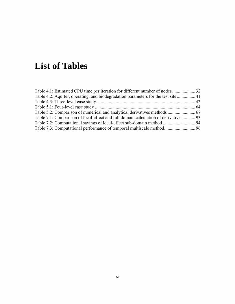
List of Tables
Table 4.1: Estimated CPU time per iteration for different number of nodes .................... 32 Table 4.2: Aquifer, operating, and biodegradation parameters for the test site ................ 41 Table 4.3: Three-level case study...................................................................................... 42 Table 5.1: Four-level case study ....................................................................................... 64 Table 5.2: Comparison of numerical and analytical derivatives methods ........................ 67 Table 7.1: Comparison of local-effect and full domain calculation of derivatives........... 93 Table 7.2: Computational savings of local-effect sub-domain method ............................ 94 Table 7.3: Computational performance of temporal multiscale method........................... 96
xii
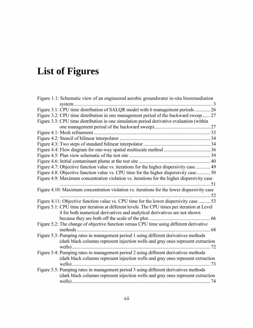
List of Figures
Figure 1.1: Schematic view of an engineered aerobic groundwater in-situ bioremediation system................................................................................................................ 3
Figure 3.1: CPU time distribution of SALQR model with 6 management periods ............. 26 Figure 3.2: CPU time distribution in one management period of the backward sweep....... 27 Figure 3.3: CPU time distribution in one simulation period derivative evaluation (within
one management period of the backward sweep)............................................... 27 Figure 4.1: Mesh refinement.................................................................................................. 33 Figure 4.2: Stencil of bilinear interpolator ............................................................................ 34 Figure 4.3: Two steps of standard bilinear interpolator ........................................................ 34 Figure 4.4: Flow diagram for one-way spatial multiscale method ....................................... 36 Figure 4.5: Plan view schematic of the test site .................................................................... 39 Figure 4.6: Initial contaminant plume at the test site ............................................................ 40 Figure 4.7: Objective function value vs. iterations for the higher dispersivity case ............ 49 Figure 4.8: Objective function value vs. CPU time for the higher dispersivity case ........... 50 Figure 4.9: Maximum concentration violation vs. iterations for the higher dispersivity case
.............................................................................................................................. 51 Figure 4.10: Maximum concentration violation vs. iterations for the lower dispersivity case
.............................................................................................................................. 52 Figure 4.11: Objective function value vs. CPU time for the lower dispersivity case .......... 53 Figure 5.1: CPU time per iteration at different levels. The CPU times per iteration at Level
4 for both numerical derivatives and analytical derivatives are not shown because they are both off the scale of the plot. ................................................... 66
Figure 5.2: The change of objective function versus CPU time using different derivative methods ................................................................................................................ 68
Figure 5.3: Pumping rates in management period 1 using different derivatives methods (dark black columns represent injection wells and gray ones represent extraction wells).................................................................................................................... 72
Figure 5.4: Pumping rates in management period 2 using different derivatives methods (dark black columns represent injection wells and gray ones represent extraction wells).................................................................................................................... 73
Figure 5.5: Pumping rates in management period 3 using different derivatives methods (dark black columns represent injection wells and gray ones represent extraction wells).................................................................................................................... 74
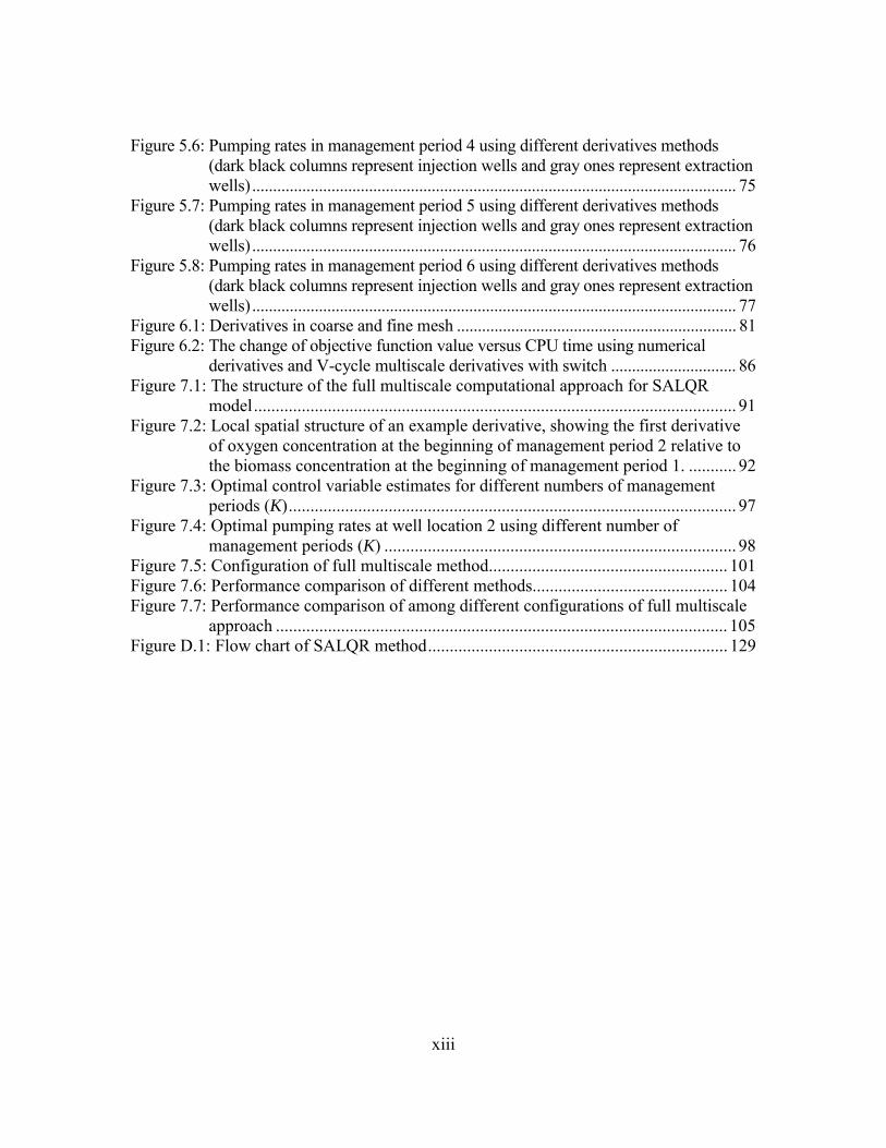
xiii
Figure 5.6: Pumping rates in management period 4 using different derivatives methods (dark black columns represent injection wells and gray ones represent extraction wells).................................................................................................................... 75
Figure 5.7: Pumping rates in management period 5 using different derivatives methods (dark black columns represent injection wells and gray ones represent extraction wells).................................................................................................................... 76
Figure 5.8: Pumping rates in management period 6 using different derivatives methods (dark black columns represent injection wells and gray ones represent extraction wells).................................................................................................................... 77
Figure 6.1: Derivatives in coarse and fine mesh ................................................................... 81 Figure 6.2: The change of objective function value versus CPU time using numerical
derivatives and V-cycle multiscale derivatives with switch .............................. 86 Figure 7.1: The structure of the full multiscale computational approach for SALQR
model............................................................................................................... 91 Figure 7.2: Local spatial structure of an example derivative, showing the first derivative
of oxygen concentration at the beginning of management period 2 relative to the biomass concentration at the beginning of management period 1. ........... 92
Figure 7.3: Optimal control variable estimates for different numbers of management periods (K)....................................................................................................... 97
Figure 7.4: Optimal pumping rates at well location 2 using different number of management periods (K) ................................................................................. 98
Figure 7.5: Configuration of full multiscale method....................................................... 101 Figure 7.6: Performance comparison of different methods............................................. 104 Figure 7.7: Performance comparison of among different configurations of full multiscale
approach ........................................................................................................ 105 Figure D.1: Flow chart of SALQR method..................................................................... 129
1
Chapter 1
Introduction Solving large-scale optimal in-situ bioremediation design problems is expected to
have huge economic benefits, yet it is constrained by the computational bottleneck in
previous existing methods. In this chapter, we introduce the background of the research
area, discuss our research goals and motivations, present major contributions of our work
and outline the rest of the dissertation.
1.1 Groundwater Contamination and Remediation Design
A range of human practices in industrial, commercial, agricultural and military
fields have contributed to groundwater contamination problems. As a result, about
300,000 to 400,000 sites have contaminated groundwater problems in the United States
(National Research Council, 1994). Typical contaminants found in the groundwater
include phenol, BTEX (Benzene, Toluene, Ethlybenzene, and Xylene) due to leaking
underground gas storage tanks and DNAPL (dense nonaqueous-phase liquids) such as
TCE (Trichloroethylene) due to the prevalent usage of industrial degreasing solvents.
Subsurface remediation is associated with tremendous cost. A recent report from
the US Environmental Protection Agency states that the remaining remediation costs for
contaminated soil and groundwater sites in the Superfund National Priorities List are
2
estimated at $187 billion in 1996 dollars (EPA, 1997). Russell et al. (1991) estimates that
about $500 billion to $1 trillion are needed in the next 30 years to cleanup the
contaminated sites in both private and public sectors to the stringent standard. Although
conventional pump-and-treat cleanup systems have been extensively used, it was found
inefficient in many scenarios due to the long remediation period and high cost. As an
alternative, in-situ bioremediation has been found to be cost-effective for cleaning up
petroleum hydrocarbon contaminants (National Research Council, 1994). This
remediation technology uses indigenous microorganisms to degrade the contaminants in-
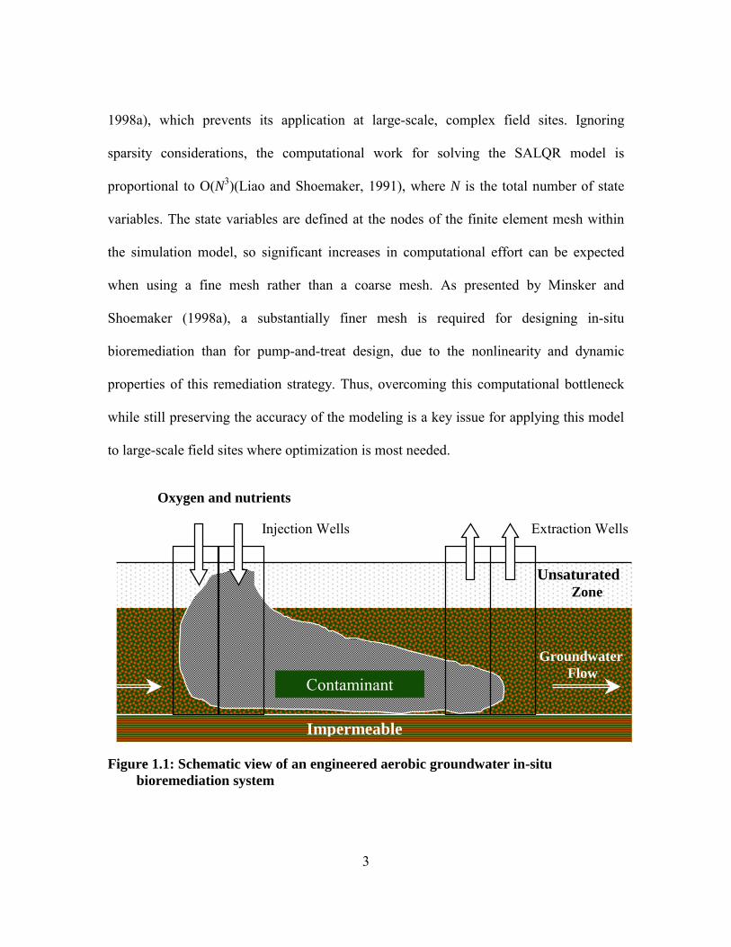
place. A typical engineered aerobic in-situ bioremediation system is shown in Figure 1.1,
where the design parameters are defined as locations and pumping rates for injection and
extraction wells. The injection wells are used to deliver oxygen and nutrients, stimulating
the growth of microorganisms and thereby accelerating degradation of pollutants. The
extraction wells are used to increase the hydraulic gradient and enhance the transport of
the injected substances.
In order to find an optimal design for in-situ bioremediation systems to achieve a
specified water quality standard at minimum cost, an optimal control method called
successive approximation linear quadratic regulator (SALQR) has been used in a coupled
simulation and optimization model (Minsker and Shoemaker, 1998b). This optimal
control model defines control variables as pumping rates and state variables as hydraulic
heads and concentrations of substrate, oxygen and biomass. The model can identify
optimal well locations and pumping rates to minimize pumping costs. However, previous
work has shown that the model is computationally intensive (Minsker and Shoemaker,
3
Impermeable
Contaminant
Groundwater Flow
Unsaturated Zone
Injection Wells Extraction Wells
Oxygen and nutrients
1998a), which prevents its application at large-scale, complex field sites. Ignoring
sparsity considerations, the computational work for solving the SALQR model is
proportional to O(N3)(Liao and Shoemaker, 1991), where N is the total number of state
variables. The state variables are defined at the nodes of the finite element mesh within
the simulation model, so significant increases in computational effort can be expected
when using a fine mesh rather than a coarse mesh. As presented by Minsker and
Shoemaker (1998a), a substantially finer mesh is required for designing in-situ
bioremediation than for pump-and-treat design, due to the nonlinearity and dynamic
properties of this remediation strategy. Thus, overcoming this computational bottleneck
while still preserving the accuracy of the modeling is a key issue for applying this model
to large-scale field sites where optimization is most needed.
Figure 1.1: Schematic view of an engineered aerobic groundwater in-situ bioremediation system
4
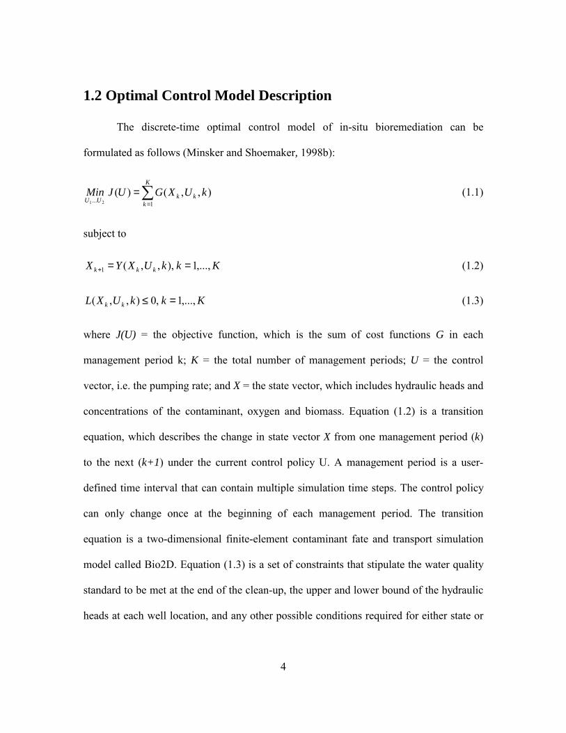
1.2 Optimal Control Model Description
The discrete-time optimal control model of in-situ bioremediation can be
formulated as follows (Minsker and Shoemaker, 1998b):
∑=
=K
kkkUU
kUXGUJMin1...
),,()(21
(1.1)
subject to
KkkUXYX kkk ,...,1),,,(1 ==+ (1.2)
KkkUXL kk ,...,1,0),,( =≤ (1.3)
where J(U) = the objective function, which is the sum of cost functions G in each
management period k; K = the total number of management periods; U = the control
vector, i.e. the pumping rate; and X = the state vector, which includes hydraulic heads and
concentrations of the contaminant, oxygen and biomass. Equation (1.2) is a transition
equation, which describes the change in state vector X from one management period (k)
to the next (k+1) under the current control policy U. A management period is a user-
defined time interval that can contain multiple simulation time steps. The control policy
can only change once at the beginning of each management period. The transition
equation is a two-dimensional finite-element contaminant fate and transport simulation
model called Bio2D. Equation (1.3) is a set of constraints that stipulate the water quality
standard to be met at the end of the clean-up, the upper and lower bound of the hydraulic
heads at each well location, and any other possible conditions required for either state or
5
control variables. Detailed formulations for the Bio2D and constraint equations can be
found in Appendix A and B, respectively.
When the model is solved using SALQR, the constraints are incorporated into the
objective function using the following penalty function:
∑∑= =
=K
k
n
qkq
q
fry1 1
001.2)],0[max( (1.4)
where y = the penalty that is added to the objective function in equation (1); fkq =
violation of the constraint q in period k, where q is any of the constraints given in
equations (1.3); nq = the number of constraints in equations (1.3); and r = a scalar penalty
weight greater than zero. The penalty weight r is initially set to a small value and the
optimal solution is found. Then the weight is increased successively by a factor of 10 and
the problem is re-solved until the constraint violations are sufficiently small.
SALQR is a variant of differential dynamic programming (DDP) in which the
second derivative of the transition equation is assumed to be zero. SALQR consists of
two iterative steps: a forward sweep and a backward sweep. An initial guess of the
control policy is needed to start the algorithm. The forward sweep runs the simulation
model to evaluate the effects of the current pumping rates, and the backward sweep
computes derivatives of the objective function and transition equation to find an
improved strategy. The algorithm stops when it converges to the optimal pumping
policy. A detailed description of the SALQR method is given in Appendix D.
6
1.3 Research Goals
The objective of this research is to develop innovative multiscale methods for
optimal in-situ bioremediation design that will enable medium- and large-scale design.
This objective will be achieved through the following goals.
Our first goal is to identify the computational bottleneck of the existing algorithm
and model. This entails computational complexity analysis both theoretically and
experimentally. Although previous works (Liao and Shoemaker, 1991; Minsker and
Shoemaker, 1998a) have done some analysis on SALQR model, the unique features of
bioremediation design have not been fully exploited. The results of this goal will provide
new insights on how we can enhance the SALQR model in general and specifically what
we should do to improve computational efficiency for optimal bioremediation design.
Our second goal is to develop innovative multiscale methods for optimal in-situ
bioremediation design and investigate the performance of each method. The motivation
for using multiscale methods in the SALQR model is to apply the general principle of
multiscale computation advocated by Brandt (1997, 2001) to overcome the computational
bottleneck posed by the current optimal in-situ bioremediation design model. These new
methods require theoretical analysis, design, implementation, and testing. Reducing the
computational effort associated with the number of nodes in space is the major target.
While these methods are developed for optimal bioremediation design, their applicability
is much broader.
Our third goal is to solve a large-scale in-situ bioremediation design with
thousands of state variables, which was not practically feasible with the previous model.
7
A case study will be solved using several multiscale methods developed in this research
and model performance will be investigated.
1.4 Contributions of this Thesis
The main contributions of this thesis are as follows:
• A detailed analysis of the SALQR model reveals the true bottleneck for optimal in-
situ bioremediation design and similar PDE-constrained optimal control models with
management period formulation to be the transition equation derivatives calculations.
• Design and implementation of efficient numerical derivatives calculation. We
exploited the calculation procedure of the one-sided divided difference derivatives
approximation of the first derivatives of transition equation with respect to the state
variables, which leads to an order of magnitude reduction in computing time for the
derivatives calculation (Liu and Minsker 2001, in press).
• Design and testing of various multiscale methods (Liu et al. 2001; Liu and Minsker
2001, in press).
• Address various modeling issues associated with optimal design of groundwater
remediation using multiscale methods, including impact of penalty terms, dispersivity
value, Peclet number, etc.
• Successful solution of large-scale case study with thousand of nodes. Our application
showed that with the full multiscale approach, a case that would have required nearly
one year to solve now only needs 9 days to converge to the optimal solution.
8
1.5 Structure of this Thesis
This thesis is organized as follows. In Chapter 2, we survey previous work on
multiscale methods in optimization, derivative-based optimization applications for
groundwater remediation design and PDE-constrained optimization problems in general.
In Chapter 3, we present detailed analysis of the SALQR model and identify the true
bottleneck of the computational performance. In Chapter 4, we develop a one-way spatial
multiscale method and apply it to different case studies. In Chapter 5, we develop an
efficient numerical derivatives approach and analyze its computational performance both
theoretically and experimentally. In Chapter 6, we present the multiscale V-cycle
derivatives method with results and analysis. In Chapter 7, we present the full multiscale
approach for optimal in-situ bioremediation design and investigate various strategies to
enhance its performance. Note that Chapters 4-6 describes the individual components of
the full multiscale method, and Chapter 7 presents the configurations and combinations
of different components of the full multiscale method. Finally, in Chapter 8, we
summarize the major findings and point out future research directions to extend and
enhance this research.
Some auxiliary materials are presented in the Appendices. In Appendix A, we
present the detail formulation of the simulation model BIO2D. In Appendix B, we
present the detailed formulation of the optimal control model for in-situ bioremediation
design. In Appendix C, we describe the first derivatives of the transition equation with
respect to the state and control variables in mathematic format. In Appendix D, we
9
present the flow chart and algorithmic description of the SALQR method with
management periods.
10
Chapter 2
Literature Review This chapter describes previous work relevant to this research. Since the
groundwater bioremediation optimal control model falls into the general category of
PDE-constrained optimization, section 2.1 gives a review of approaches taken to solving
such problems. Section 2.2 overviews previous work on multiscale methods for solving
PDEs and optimization problems. A brief summary of previous optimal groundwater
remediation design studies is given in Section 2.3. Finally, a summary of the literature
review is given in Section 2.4.
2.1 PDE-constrained Optimization Problems
The optimal groundwater bioremediation design problem considered in this work
(see Equations (1.1) to (1.4) in Chapter 1) is an example of PDE-constrained
optimization. Solving an optimization problem governed by PDEs is generally much
harder than solving PDEs alone, since solving PDEs is only a subproblem associated with
optimization. In the optimization problem, the governing PDEs are called state or
transition equations. As methods for solving large-scale PDE simulation models with
millions of unknowns have matured, interest in solving large-scale PDE-constrained
11
problems arising in many areas of science and engineering has increased. Such
optimization problems usually have two forms: inverse modeling and optimal design or
control modeling. Inverse problems involve calibrating parameters in the simulation
model using the observed known data. For example, a typical inverse problem in
groundwater modeling may require estimation of hydraulic conductivity and storativity.
Recent development and methods reviews for the groundwater inverse problem can be
found in the literature (see, e.g., Woodbury and Ulrych 2000; Schulz et al. 1999; Zio
1997; Ferraresi et al. 1996; McLaughlin and Townley 1996).
In optimal design or optimal control modeling, literature is sparse for tackling
large-scale problems. Most papers found in the literature are on optimal shape design or
optimal flow boundary control where the PDE constraints are usually the Navier-Stokes
or Euler flow equations and the objective function is an integral equation. A nonlinear
programming method called Sequential Quadratic Programming (SQP) (Boggs and Tolle
2000; Arnold and Puta 1994) is typically used to solve the optimization problem where
the PDEs are treated as equality constraints and incorporated into the objective function
using Lagrange multipliers. Biros and Ghattas (1999, 2000) proposed a parallel version of
Newton-Krylov solver to solve the resulting large-scale Karush-Kuhn-Tucker (KKT)
system after applying the first-order optimality condition to an optimal flow control
problem. A variant of SQP method was used to solve this problem with good scalability.
However, no inequality constraints for state variables or control variables are present in
their optimization problems. In addition, the control variables are located in the boundary
whose dimension can be changed with different discretizations (hence the name optimal
12
boundary control or optimal shape design) and an adjoint state equation was used to
calculate the gradient. These characteristics are quite different from the optimal control
model of groundwater bioremediation used in this research.
Another active theoretical research area is applying automatic differentiation
techniques for solving optimal control problems. Hovland et al. (2000) used automatic
differentiation to generate the Hessian matrix for an SQP-like nonlinear optimization
algorithm to solve an optimal boundary control problem similar to Biros and Ghattas
(1999, 2000). Bartholomew-Biggs et al. (2000) and Christianson and Bartholomew-Biggs
(2000) used automatic differentiation to evaluate the Newton direction for a discrete-time
optimal control algorithm called Pantojas algorithm (Pantoja 1988). Only a theoretical
analysis was performed for using automatic differentiation with Pantojas algorithm,
without any real-world application.
2.2 Multiscale Methods in Simulation and Optimization
To enable large-scale solution of PDEs and PDE-constrained optimal design or
control problems, multiscale methods have attracted considerable research interest in the
past years. The term "multiscale method" has been used extensively in the literature
within different contexts. The standard multigrid method is probably the most well-
known multiscale method. The scope of applicability of multiscale methods is
impressive, as indicated by Brandt (1997, 2001) in his survey paper. The most
extensively researched application of multiscale methods is as fast partial differential
equation (PDE) solvers known as multigrid solvers. As shown by many researchers (see,
13
e.g., Brandt 1977; Hackbusch 1979; Douglas 1984; Mavriplis and Jameson 1990),
multigrid solvers exhibit a convergence rate for solving PDEs that is independent of the
number of unknowns in the discretized system. In the following, we first sketch the basic
idea of multigrid solvers and their applications in groundwater simulation modeling. We
then review the multiscale methods applied in solving various optimization problems.
2.2.1 Multigrid Solvers for Groundwater Simulation Modeling
To understand how multigrid solvers work, it is necessary to understand the
concept of error first. Expressed in terms of a discrete Fourier series, the error (the
difference between the true solution and an approximated iterative solution) can be
represented by various Fourier components of different wave numbers. Oscillatory error
components refer to those with small wavelength, while smooth error components refer
to those with large wavelength. There are two key components in multigrid solvers:
smoothers and coarse grid correction. The smoothers are usually relaxation methods,
such as Gauss-Seidel, which can damp out the high frequency (i.e., oscillatory) error
components quite quickly but cannot effectively reduce the low frequency (i.e., smooth)
error components. However, the high or low frequency components of the error are
relative to the grid on which the solution is defined. Smooth components on a fine grid
appear oscillatory when sampled on a coarse grid. The idea of coarse grid correction
takes advantage of the grid-dependent feature of the error component. By restricting the
residual on the fine grid to the coarse grid via a restriction operator, the error equation on
the coarse grid is solved to get an error correction for the fine grid solution. After
interpolating the coarse grid correction back to the fine grid via an interpolation operator
14
and adding the correction to the approximated solution, the low frequency error
components on the fine grid now should also be reduced significantly, which is why
multigrid solvers are so effective. This process can be repeated until some convergence
criterion is met. An important aspect of the multigrid solvers is that the coarse grid
solution can be approximated by recursively using the two-grid (coarse and fine) iteration
idea. That is, on the coarse grid, relaxation is performed to reduce high frequency
components of the errors followed by the restriction of the correction equation to yet an
even coarser grid, and so on. Depending on how the algorithm moves up and down the
grids, there are many variants of multigrid solvers, such as V-cycle, W-cycle and full
multigrid. Detailed theoretical and numerical discussions of multigrid solvers can be
found in Stüben and Trottenberg (1982), Hackbusch (1985) and Briggs(1987). The book
by Joppich and Mijalković (1993) is especially helpful for engineers modeling process
simulation.
Several applications of multigrid solvers in groundwater flow and solute fate and
transport simulation can be found in the literature. Mckeon and Chu (1987) used a full
approximation scheme (FAS) of multigrid methods to solve a nonlinear two-dimensional
flow equation discretized by the finite difference method. Beckie et al. (1993) found that
mixed finite element methods combined with domain decomposition and a multigrid
solver can be effectively used to solve systems with over 4 million unknowns and
strongly heterogeneous conductivity for their two-dimensional saturated groundwater
flow simulation. Saied and Mahinthakumar (1998) presented parallel multigrid solvers
for large-scale linear systems arising from the finite-element discretization of a three-
15
dimensional steady-state groundwater flow problem. Cheng et al. (1998) used multigrid
methods to solve two existing three-dimensional finite-element subsurface flow and
transport models. Li et al. (2000) combined multigrid methods and adaptive local grid
refinement to solve a three-dimensional density-dependent groundwater flow and
substrate transport model. Jones and Woodward (2001) used multigrid methods as
preconditioners and Newton-Krylov solvers to solve a nonlinear, variably saturated
groundwater flow problem. Note that all of these papers dealt with only a simulation
model, but not a coupled simulation and optimization model, so standard multigrid
solvers could be used.
2.2.2 Multiscale Methods for Optimization Problems
Solving optimal control or optimization problems using multiscale methods,
however, is much more difficult than solving PDEs alone. One of the multiscale optimal
control methods, called "one-shot" full multigrid minimization method, can be found in
the field of optimal shape design (OSD) of aerodynamic systems, such as designing wing
shapes (Taasan 1991; Arian and Taasan 1994a). This optimal control problem is
governed by a set of elliptic equations and is solved by using an adjoint method based on
a Lagrange multiplier method. The control variables are located on the boundary. Again,
the state equation is treated as an equality constraint and the resulting KKT linear system
was solved using multigrid solvers. Their "one-shot" method was applied to a two-
dimensional OSD problem with a finite element discretization and showed efficient
convergence behavior that was independent of mesh sizes (Arian and Taasan 1994b).
Schulz and co-workers (Dreyer et al. 2000; Maar and Schulz 2000) developed similar
16
multigrid approaches as Taasan (1991) to solve the resulting KKT linear system. Both
the SQP-like optimization algorithm and interior point optimization algorithm were used
in their papers. The applications presented in their papers are again optimal shape design
problems arising in structural truss topology design and turbine blade design.
Nash and his co-workers (Nash 2000; Lewis and Nash 2000) proposed a multigrid
approach for discretized optimization problems constrained by PDEs. Their method
focuses on applying the multigrid method to the whole optimization problem. However,
there are no inequality constraints present in their example problems and the governing
equation is a single PDE, not coupled systems of PDEs with nonlinearity. The objective
function in their examples is explicitly related to the discretization of the state variables,
so that at different level of discretization, a different value of objective function can be
obtained. This type of objective function is not applicable to the groundwater
bioremediation optimal control problem considered in this work.
Within the context of stochastic control, several papers have used multigrid
methods. Akian et al. (1988) developed a full multigrid Howard (FMGH) algorithm for
solving a continuous-time stochastic control problem using dynamic programming.
Hoppe (1986) applied a multigrid method for solving Hamilton-Jacobi-Bellman
equations arising in a continuous-time optimally controlled stochastic process. Both
Akian and Hoppe used multigrid methods as a PDE solver to solve the elliptic PDE (the
objective function) in their problems. Chow and Tsitsiklis(1991) presented an optimal
one-way multigrid version of a successive approximation algorithm for solving a
discrete-time continuous-state discounted-cost Markov decision problem, in which the
17
objective function is an integral equation. The problem is solved on a coarse grid initially
and then the coarse grid solution is used as a starting point for the solution on a finer grid.
Their method goes from the coarsest grid to the finest grid with most of the work taking
place on coarse grids.
For these stochastic control problems, the multigrid methods are used in the
objective function space, where the objective function (elliptic PDE or integral equations)
is the computational bottleneck. However, in our problem, the computational burden is
associated with calculating derivatives in the state variable space (see Chapter 3 for
details). The number of control variables (pumping rates) is far less than that of state
variables (hydraulic heads and concentrations at each node of the numerical mesh).
Unlike previous multiscale studies, the objective function in our problem is quite easy to
compute and requires no discretization. Hence, our method focuses on reducing the
computational effort associated with state-space computations.
Another example of multiscale optimization is in neural networks optimization
(Mjolsness et al., 1991). A general neural network objective function for continuous
neural variables is composed of a sum of linear, quadratic, and cubic terms. An ordinary
network can be transformed into a multiscale network by the addition of smaller and
cheaper approximating networks at successive scales, with associated objective functions.
Mjolsness and co-workers achieved a speedup of a constant factor (between 2 and 5),
which is independent of the problem size, compared with the original single-scale
computational work. Again note that this type of multiscale optimization also deals with
only the objective function space.
18
There exists another well-known research field called multilevel optimization
(Migdalas et al.1998) that is sometimes confused with multiscale methods. A typical
multilevel optimization problem has a hierarchy of decision-makers and decisions are
made at different levels in this hierarchy. Thus, this approach is entirely different from
the above-mentioned multiscale methods.
2.3 Applications for Groundwater Remediation Design
This section briefly reviews the optimization methods that have been used for
pump-and-treat and in-situ bioremediation design. The focus of this review is on
applications of derivative-based optimization techniques, since that is the approach for
which the multiscale methods developed in this work are most applicable.
Optimization techniques have been applied primarily to traditional pump-and-treat
remediation design. Derivative-based nonlinear programming methods include the work
by Ahlfeld et al. (1988), Merckx (1991), Bear and Sun (1998) and many others. SALQR
(Chang et al. 1992; Mansfield and Shoemaker 1999) and SALQR with management
periods or quasi-Newton methods (Culver and Shoemaker 1992, 1993) have also been
used to find time-varying optimal pumping policies. Other applications of SALQR and
DDP in the water resources field include multireservoir control (Murray and Yakowitz,
1979), groundwater quantity management (Jones et al., 1987), estuarine management (Li
and Mays, 1995) and sedimentation control in reservoir-river systems (Carriaga and
Mays, 1995).
19
In dealing with the calculation of the derivatives, analytical derivatives (Chang et
al. 1992; Culver and Shoemaker 1992; Mansfield and Shoemaker 1999), discrete adjoint
method (Merckx, 1991; Ahlfeld, 1988), discrete sensitivity equations method (Merckx
1991) and finite-difference approximations (Ahlfeld et al.1986; Gorelick et al.1984) have
been used. The derivative calculations required a substantial amount of computing time
in all of these applications. For example, Ahlfeld et al. (1988) showed that for a test case
in his paper, about 11 hours were devoted to the calculation of the derivatives using the
adjoint sensitivity method and 15.9 hours for running the simulation model. Only a
fraction of 1 hour was used for the remaining operations of the optimization algorithm.
Whiffen (1995) showed that one-sided finite difference approximations to the derivatives
needed in SALQR took about 29 times the computing time required to compute the same
derivatives analytically, and that derivatives computed using automatic differentiation
took about 3 times the CPU of analytical derivatives.
Due to the nonlinearities related to biomass growth, a substantially finer mesh is
required for in-situ bioremediation than for pump-and-treat design. This causes the
computational challenges mentioned in Chapter 1. Minsker and Shoemaker's SALQR
model (1996) was the first application of formal optimization methods to in-situ
bioremediation design. Yoon and Shoemaker (1999) compared the computational
performance of eight different optimization methods, including SALQR, for groundwater
bioremediation design, and claimed that SALQR was consistently faster on all of the
example problems, but is not necessarily the most accurate method. However, note that
the size of the two examples presented in Yoon and Shoemaker's paper is rather small
20
(case 1 only has 90 grid points and case 2 only has 162 grid points). As mentioned in
Chapter 1, the poor scalability of the SALQR algorithm prevents application to large-
scale problems, but has less effect when the problem size is small. Investigation of
multiscale technique to allow application SALQR to middle- and large-scale problems is
the focus of this research work.
2.4 Summary
In this chapter, we have surveyed existing work on PDE-constrained optimization
problems, multiscale methods in simulation and optimization, and derivative-based
optimal design for groundwater pump-and-treat and in-situ bioremediation. As a frontier
problem in computational science and engineering, PDE-constrained optimization poses a
computational challenge even for the most advanced supercomputing power available
today. Multiscale methods have been found very efficient for handling very large-scale
simulation modeling, but very few examples were found in PDE-constrained
optimization. In subsequent chapters, we develop innovative multiscale methods for
optimal design of groundwater in-situ bioremediation. Solving large-scale optimal
bioremediation design problems is expected to be highly rewarding, since substantial cost
savings could be achieved at large complex field sites if optimal designs can be used. The
methods developed in this work are also expected to be applicable for other PDE-
constrained optimization problems.
21
Chapter 3
Analysis of Computational Effort of Optimal In-Situ Bioremediation Design This chapter will analyze the computational effort associated with both the
forward sweep and backward sweep in the SALQR method, which will reveal the exact
computational bottleneck of the existing model.
3.1 Previous Work
Earlier work on the computational complexity analysis of SALQR and DDP has
mainly focused on demonstrating the linear growth rate of the algorithm with respect to
the time steps, although the cubic growth rate of the computational complexity with
respect to the number of state variables and control variables has also been shown in the
theoretical analysis (Yakowitz and Rutherford 1984; Liao and Shoemaker 1991).
However, their analysis has mainly focused on the steps that involve updating the search
directions, but not the derivative calculations (see Appendix D for more details on these
steps). Analytical derivatives have been used in both pump-and-treat and bioremediation
design in previously published SALQR models for groundwater remediation. For the
pump-and-treat remediation design, Mansfield et al. (1998) and Mansfield and
22
Shoemaker (1999) reduced the computational complexity of calculating the first
derivatives of the transition equation with respect to the state variables by utilizing the
sparsity of the matrices. However, no complexity analysis for the management period
derivative calculations was presented in their papers. Culver and Shoemaker (1992)
presented derivative calculations for both simulation period derivatives and management
period derivatives in pump-and-treat design. They found that in their application the
calculation of the derivatives over management period requires less work than in the
general case. No complexity analysis in terms of growth rate was given for the
management period derivatives, although the overall cost for calculating derivatives was
described as O(N3), where N is the number of state variables. Minsker and Shoemaker
(1996) presented detailed derivation of the analytical derivatives of the bioremediation
transition equation used in this work with respect to the state and control variables, but no
computational complexity analysis was presented. Minsker and Shoemaker (1998a)
performed experimental analysis to show that up to 98% of the computing time was used
in the backward sweep. However, no detailed analysis was presented to discover the
exact computational bottleneck.
SALQR is a derivative-based optimization technique that requires the first and
second derivatives of the objective function, penalty function, and constraints and the
first derivatives of the transition equation. Derivatives of the objective function, penalty
function and constraints are usually easy to calculate and thus analytical derivatives are
used. Since the transition equation is often a numerical model such as a finite-element or
finite-difference simulation model for groundwater remediation design, it is a challenging
23
and computationally expensive task to calculate the analytical derivatives of the
simulation model. The following sections present analysis that reveals the exact
computational bottleneck of the bioremediation optimal control model studied in this
work.
3.2 Theoretical Analysis of the Computational Effort
As discussed in Chapter 1 (and detailed in Appendix D), SALQR is an iterative
method that consists of two steps: forward sweep and backward sweep. The forward
sweep simply involves running the simulation model under the current pumping policy.
To approximate the original continuous partial difference equations given in Appendix A,
the simulation model uses a linear basis function in space with an approximation
accuracy order of O(h)), where h is the spatial grid size. A fully-implicit backward-Euler
differencing method is used in the time stepping scheme (except for the reaction terms,
which are explicit) with an approximation accuracy order of O(t), where t is the
simulation time step. The current model uses a banded Gaussian elimination direct solver
in LAPACK (subroutines DGBSV or DGBTRF and DGBTRS) to solve the discretized
system of equations. The complexity associated with these direct solvers is O((s+1)2N),
where s is the bandwidth (e.g. for a tri-diagonal matrix, s=1; see the definition in Iserles's
book (Iserles 1996) ) and N is the total number of state variables. For this application, the
forward sweep consumes less than 5% of the total CPU time for solving the SALQR
model.
24
In the backward sweep, a quadratic approximation of the "cost to go" function,
which is the total cost from the current management period to the end, is made at each
management period running backwards from K to 1, where K is the number of the last
management period. Several matrices, such as Ak, Bk, Ck, Dk, Ek., (see Appendix D for
the definition of these matrices), must be calculated in each management period during
one iteration of the optimization procedure. However, these matrices themselves require
the first and second derivatives of the transition equation (i.e. ∂Y/ ∂X and ∂Y/∂U in
Appendix C), the objective function, and the constraints to be evaluated. The derivatives
of the objective function and constraints are easy to calculate analytically, but the
derivatives of the transition equation are quite complex. Hence, the transition equation
(i.e., simulation model) is linearized when calculating the derivatives so that at each
management period a linear quadratic regulator (LQR) is solved using the first-order
necessary condition of optimality. With this approximation, the backward sweep is
equivalent to the stagewise Newton's method (Murray and Yakowitz 1984; Dunn and
Bertsekas 1989; Pantoja 1988). However, the linearization of the transition equation
leads to a deterioration of the convergence rate of the DDP method, which has a quadratic
convergence rate, because the Hessian matrix of the original optimal control problem
(OCP) will not typically come close to that of the OCP with the linearized transition
equation (Murray and Yakowitz, 1984).
Previous numerical experiments (Minsker and Shoemaker1998a) found that about
95~98% of the total computing time were spent on the backward sweep. Our further
analysis of the CPU time distribution found that more than 90% of the total time on the
25
backward sweep was actually used on the calculation of the first derivatives of the
transition equation with respect to the state variables and control variables over each
simulation period and management period. This is the bottleneck of this model.
This computational bottleneck is caused by the current two-step method used to
calculate the first derivatives of the transition equation. The first step of the method is to
calculate the derivatives within each simulation time period, which involves a matrix
inversion and multiplication of a dense and a banded matrix. These operations involve
O(N3) computational complexity (see equations (21), (26)-(28), (32), (35)-(37), (41),
(44)-(46) and (50) in Minsker and Shoemaker 1996), where N is the total number of non-
Dirichlet state variables. The second step of the method is to use the product rule for
differentiation to obtain derivatives across each management time period, since each
management period consists of several simulation time steps (the number of simulation
time steps within one management period can be denoted as d). This involves
multiplication of matrices of dimension N by N, with O(N3) computational complexity
(see equations (13) and (14) in Culver and Shoemaker 1992). The sparsity pattern was
lost in these approaches because of the matrix inversion and multiplications. See
Appendix C for the details of the first derivative calculation at each simulation period and
management period.
To find the updated control policy in each management period, matrices Ak, Bk,
Ck, Dk, Ek , Pk, Qk (see Appendix D for the definition of these matrices) must be
calculated. However, only matrix Ak has a computational effort of O(N3); others are only
on the order of O(N2m), or O(Nm2) or O(m3), where m is the number of control variables.
26
Since the number of state variables ( N ) is usually much larger than that of control
variables (m) for this application, we know that N3>>mN2>>Nm2>>m3. Although the
calculation of matrix Ak has a computational complexity of O(N3), it is only calculated
once in each management period. Thus, its contribution to the total computing time is less
important than the calculation of the first derivatives of the transition equation. This can
be further demonstrated by the subsequent experimental analysis.
3.3 Experimental Analysis of the Computational Efforts
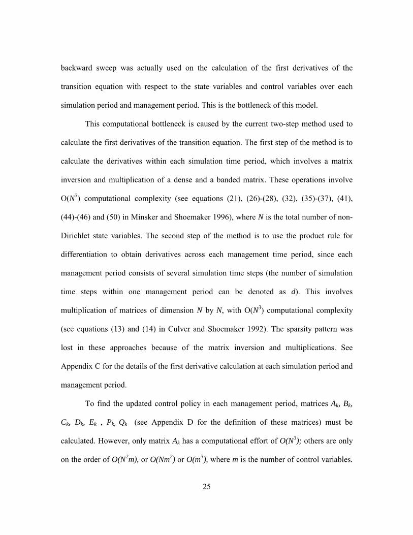
To illustrate the bottleneck of the computing time, the CPU time distribution is
derived for an example with 6 management periods. Each management period consists of
30 simulation time steps. The number of non-Dirichlet state variables N is 335 and the
dimension of the control variables m is 5.
Other operations 2%
Forward sweep 3% Backward sweep 93%
Figure 3.1: CPU time distribution of SALQR model with 6 management periods
27
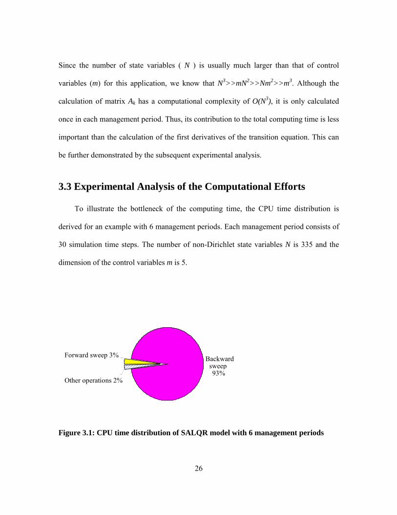
Minimization and update of
the control policy 6%
Derivatives evaluation (including simulation and management period derivatives)
94%
Figure 3.2: CPU time distribution in one management period of the backward sweep
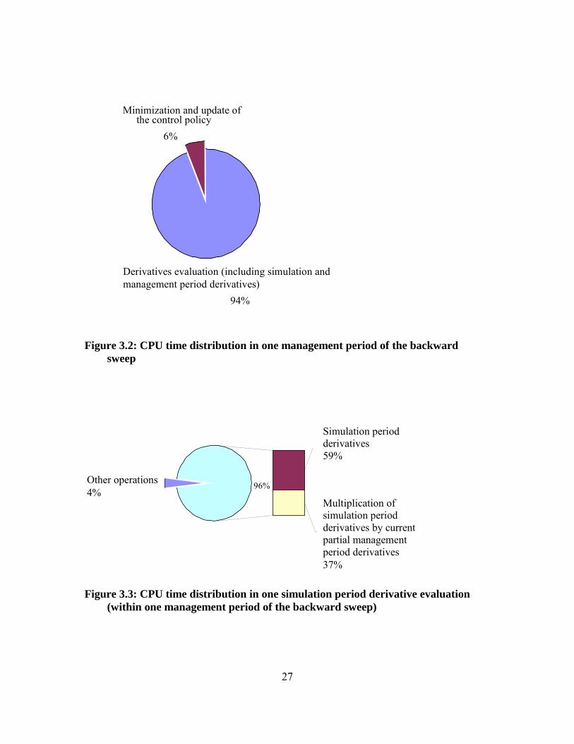
Other operations 4%
96%
Multiplication of simulation period derivatives by current partial management period derivatives 37%
Simulation period derivatives 59%
Figure 3.3: CPU time distribution in one simulation period derivative evaluation
(within one management period of the backward sweep)
28
As can be seen in Figure 3.1, about 93% of the total computing time was spent on
the backward sweep, while only 3% of the total time was used in the forward sweep.
Figure 3.2 shows that within each management period of the backward sweep, about 94%
of the computing time was used to calculate the first derivatives of the transition equation
with respect to the control variables and state variables, which includes the calculation of
both the simulation and management period derivatives. Figure 3.3 shows that in one
simulation period, about 59% of the computing time was used to calculate the current
simulation period derivative, which is the first step in the current two-step method
described above, while 37% of the time was used to obtain the partial management period
derivatives, which is the second step in the two-step method.
3.4 Summary
A detailed analysis presented in this chapter reveals the exact bottleneck of the
SALQR model, which is the two-step analytical derivatives calculation. The management
period formulation is essential for in-situ bioremediation, because the short simulation
periods (such as a half day) required to accurately model in-situ bioremediation would be
impractical for changing the pumping rates. However, the two-step analytical
management period derivatives approach developed in previous work exhibits a
computational complexity of O(N3), where N is the number of state variables. Our
experimental results further showed that more than 90% of the CPU time was spent on
the derivatives calculation. The multiscale methods presented in subsequent chapters are

29
developed to alleviate this computational bottleneck and enable large-scale solution of
bioremediation design problems.
30
Chapter 4
One-way Spatial Multiscale Method This chapter describes the one-way spatial multiscale method for optimal in-situ
bioremediation design. As shown in the previous chapters, the fundamental barrier of
applying the current optimal control model to large-scale groundwater remediation is the
cubic growth rate of the computing time with respect to the number of state variables. In
order to overcome this barrier, several spatial multiscale methods are developed and
tested in Chapters 4-7. This chapter presents the first method, which solves the
optimization problem by using a coarse grid optimal solution as a starting point for finer
grid optimization. Since this method is designed to treat the optimization problem as a
whole, it is applicable to any PDE-constrained optimization problem as long as the
governing PDEs can be spatially discretized into different scales.
4.1 Description of the Methodology
4.1.1 Basic Idea
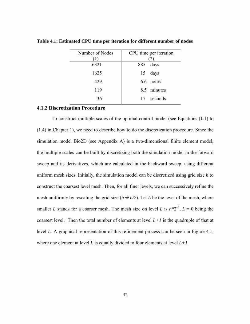
As indicated by Minsker and Shoemaker (1998a), the single-grid version of their
model is computationally intensive and field scale modeling is not possible at present.
Table 4.1 lists the estimated computing time for one iteration of the single-grid model
31
with different numbers of nodes. The estimated CPU time is based on an NCSA
SGI/Cray Origin2000 supercomputer using serial code. It's clear that the computing time
increases dramatically when the total number of nodes in the finite element mesh
increases. This means that even with cutting edge computing power, a relatively large-
scale domain cannot be modeled in a reasonable time period. However, Table 4.1 also
tells us that if initially we do some iterations on the coarse mesh and then use the result of
control policy obtained on the coarse mesh as an initial guess on the finer mesh, we could
save some computing time in the fine mesh. In principle, this idea is called nested
iteration. As stated by Joppich and Mijalković (1993), nested iteration involves finding a
reasonable initial guess for a finer grid iteration by computing approximations on coarser
grids that are successively interpolated to finer grids. This idea has been used
successfully to solve PDEs within the full multigrid (FMG) method in the literature
(Joppich and Mijalković 1993). A variant of FMG, one-way multigrid, proceeds "one-
way" from a coarse level to a fine level by interpolating the results at the coarser level to
a finer one without coarse grid correction. As pointed out by Douglas (1996), one-way
multigrid algorithm has been the standard method for combustion problems for at least 25
years and is very effective for hard engineering problems. The nested iteration principle
was also applied together with successive over relaxation (SOR) method for solving a
two-dimensional Laplace equation (Kronsjö and Dahlquist 1971). We developed a one-
way spatial multiscale method that combines the nested iteration principle with the
SALQR method. Details on the method are given in the following sections.
32
Table 4.1: Estimated CPU time per iteration for different number of nodes
Number of Nodes (1)
CPU time per iteration (2)
6321 885 days
1625 15 days
429 6.6 hours
119 8.5 minutes
36 17 seconds
4.1.2 Discretization Procedure
To construct multiple scales of the optimal control model (see Equations (1.1) to
(1.4) in Chapter 1), we need to describe how to do the discretization procedure. Since the
simulation model Bio2D (see Appendix A) is a two-dimensional finite element model,
the multiple scales can be built by discretizing both the simulation model in the forward
sweep and its derivatives, which are calculated in the backward sweep, using different
uniform mesh sizes. Initially, the simulation model can be discretized using grid size h to
construct the coarsest level mesh. Then, for all finer levels, we can successively refine the
mesh uniformly by rescaling the grid size (h! h/2). Let L be the level of the mesh, where
smaller L stands for a coarser mesh. The mesh size on level L is h*2-L, L = 0 being the
coarsest level. Then the total number of elements at level L+1 is the quadruple of that at
level L. A graphical representation of this refinement process can be seen in Figure 4.1,
where one element at level L is equally divided to four elements at level L+1.
33
!
Level L Level L+1
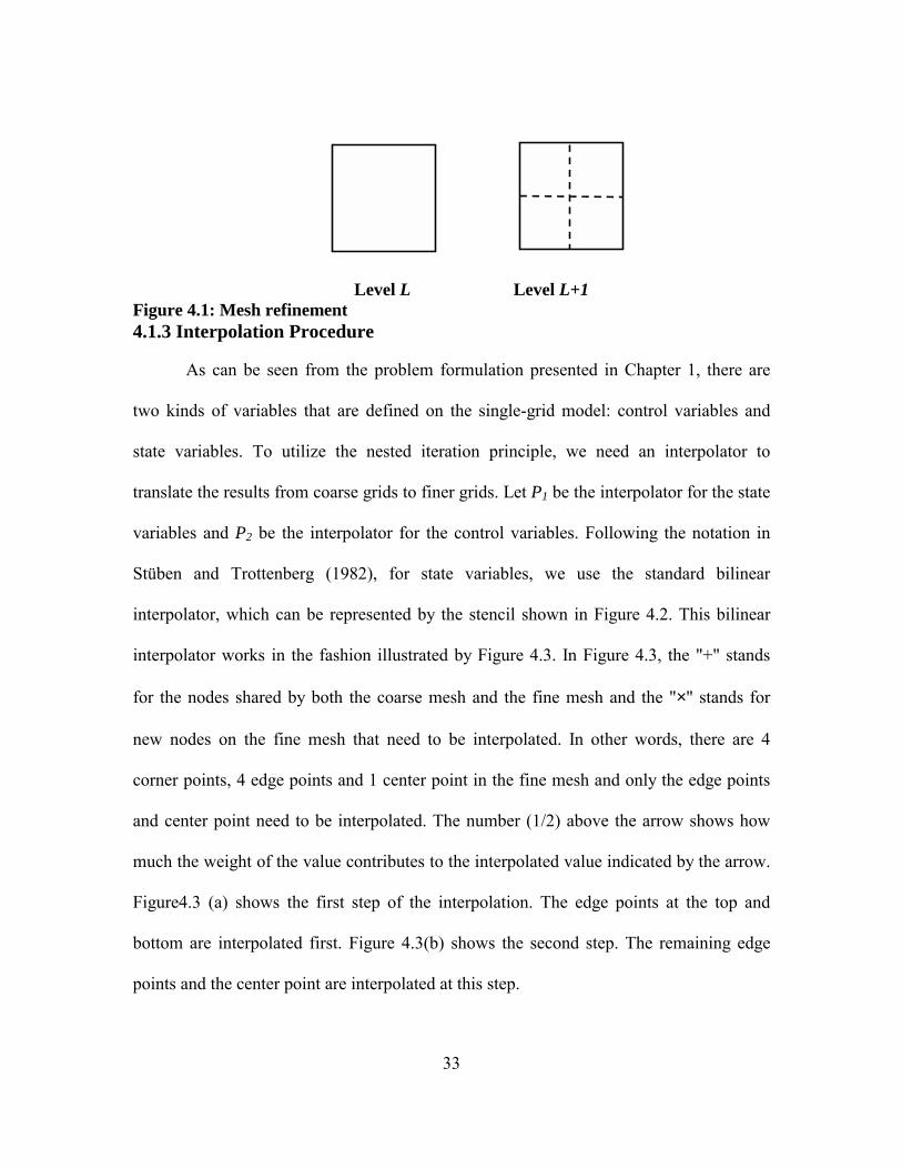
Figure 4.1: Mesh refinement 4.1.3 Interpolation Procedure
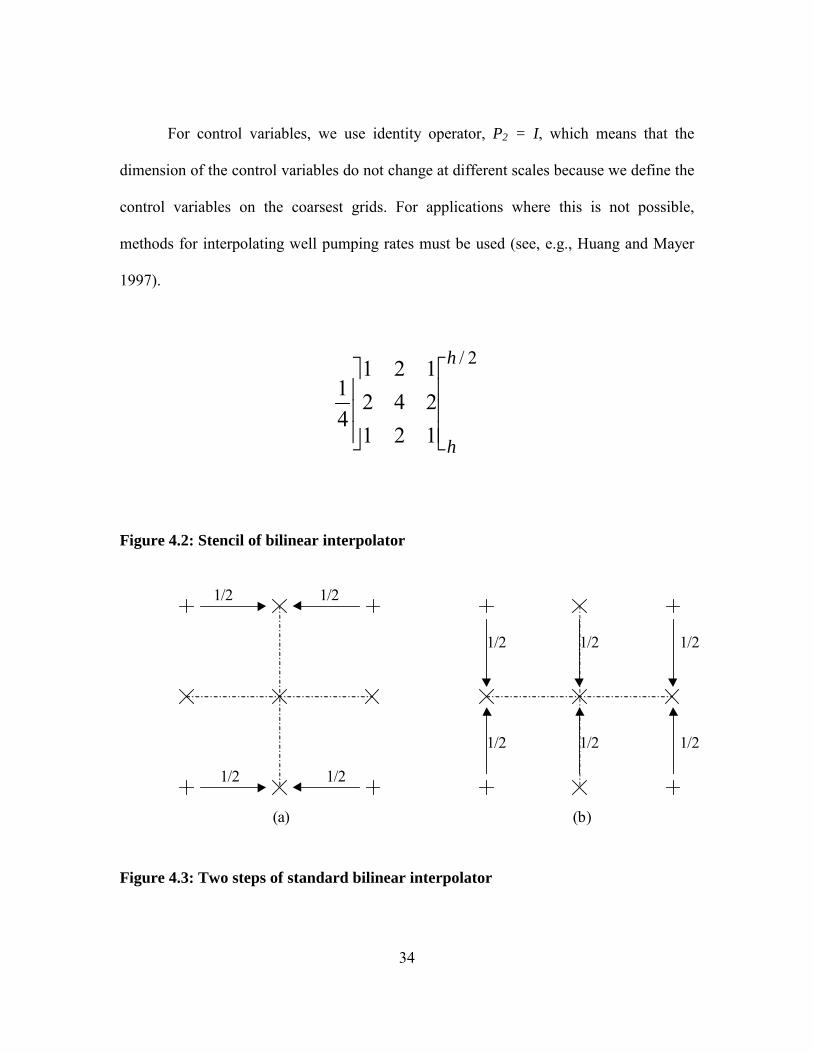
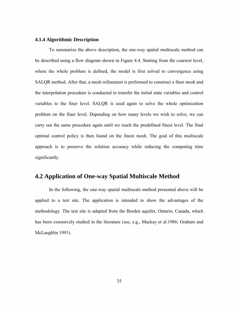
As can be seen from the problem formulation presented in Chapter 1, there are
two kinds of variables that are defined on the single-grid model: control variables and
state variables. To utilize the nested iteration principle, we need an interpolator to
translate the results from coarse grids to finer grids. Let P1 be the interpolator for the state
variables and P2 be the interpolator for the control variables. Following the notation in
Stüben and Trottenberg (1982), for state variables, we use the standard bilinear
interpolator, which can be represented by the stencil shown in Figure 4.2. This bilinear
interpolator works in the fashion illustrated by Figure 4.3. In Figure 4.3, the "+" stands
for the nodes shared by both the coarse mesh and the fine mesh and the "×" stands for
new nodes on the fine mesh that need to be interpolated. In other words, there are 4
corner points, 4 edge points and 1 center point in the fine mesh and only the edge points
and center point need to be interpolated. The number (1/2) above the arrow shows how
much the weight of the value contributes to the interpolated value indicated by the arrow.
Figure4.3 (a) shows the first step of the interpolation. The edge points at the top and
bottom are interpolated first. Figure 4.3(b) shows the second step. The remaining edge
points and the center point are interpolated at this step.
34
For control variables, we use identity operator, P2 = I, which means that the
dimension of the control variables do not change at different scales because we define the
control variables on the coarsest grids. For applications where this is not possible,
methods for interpolating well pumping rates must be used (see, e.g., Huang and Mayer
1997).
2/
121242121
41
h
h
Figure 4.2: Stencil of bilinear interpolator
1/2 1/2
1/2 1/2
1/2 1/2
1/2
1/2
1/2 1/2
(a) (b)
Figure 4.3: Two steps of standard bilinear interpolator
35
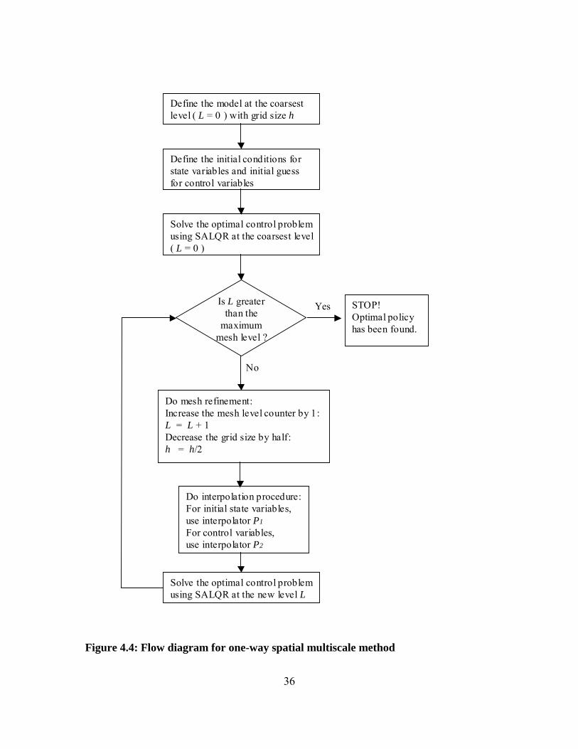
4.1.4 Algorithmic Description
To summarize the above description, the one-way spatial multiscale method can
be described using a flow diagram shown in Figure 4.4. Starting from the coarsest level,
where the whole problem is defined, the model is first solved to convergence using
SALQR method. After that, a mesh refinement is performed to construct a finer mesh and
the interpolation procedure is conducted to transfer the initial state variables and control
variables to the finer level. SALQR is used again to solve the whole optimization
problem on the finer level. Depending on how many levels we wish to solve, we can
carry out the same procedure again until we reach the predefined finest level. The final
optimal control policy is then found on the finest mesh. The goal of this multiscale
approach is to preserve the solution accuracy while reducing the computing time
significantly.
4.2 Application of One-way Spatial Multiscale Method
In the following, the one-way spatial multiscale method presented above will be
applied to a test site. The application is intended to show the advantages of the
methodology. The test site is adapted from the Borden aquifer, Ontario, Canada, which
has been extensively studied in the literature (see, e.g., Mackay et al.1986; Graham and
McLaughlin 1991).
36
Define the model at the coarsest level ( L = 0 ) with grid size h
Define the initial conditions for state variables and initial guess for control variables
Solve the optimal control problem using SALQR at the coarsest level ( L = 0 )
Is L greater than the
maximum mesh level ?
No
Yes
Do mesh refinement: Increase the mesh level counter by 1: L = L + 1 Decrease the grid size by half: h = h/2
Do interpolation procedure: For initial state variables, use interpolator P1 For control variables, use interpolator P2
Solve the optimal control problem using SALQR at the new level L
STOP! Optimal policy has been found.
Figure 4.4: Flow diagram for one-way spatial multiscale method
37
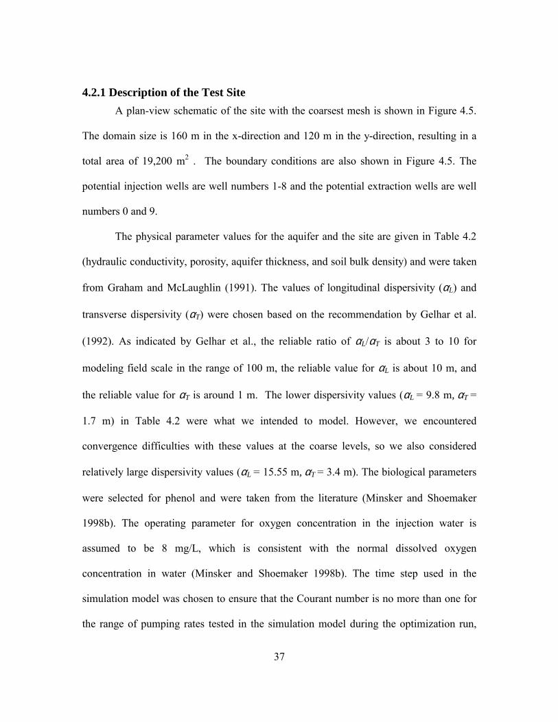
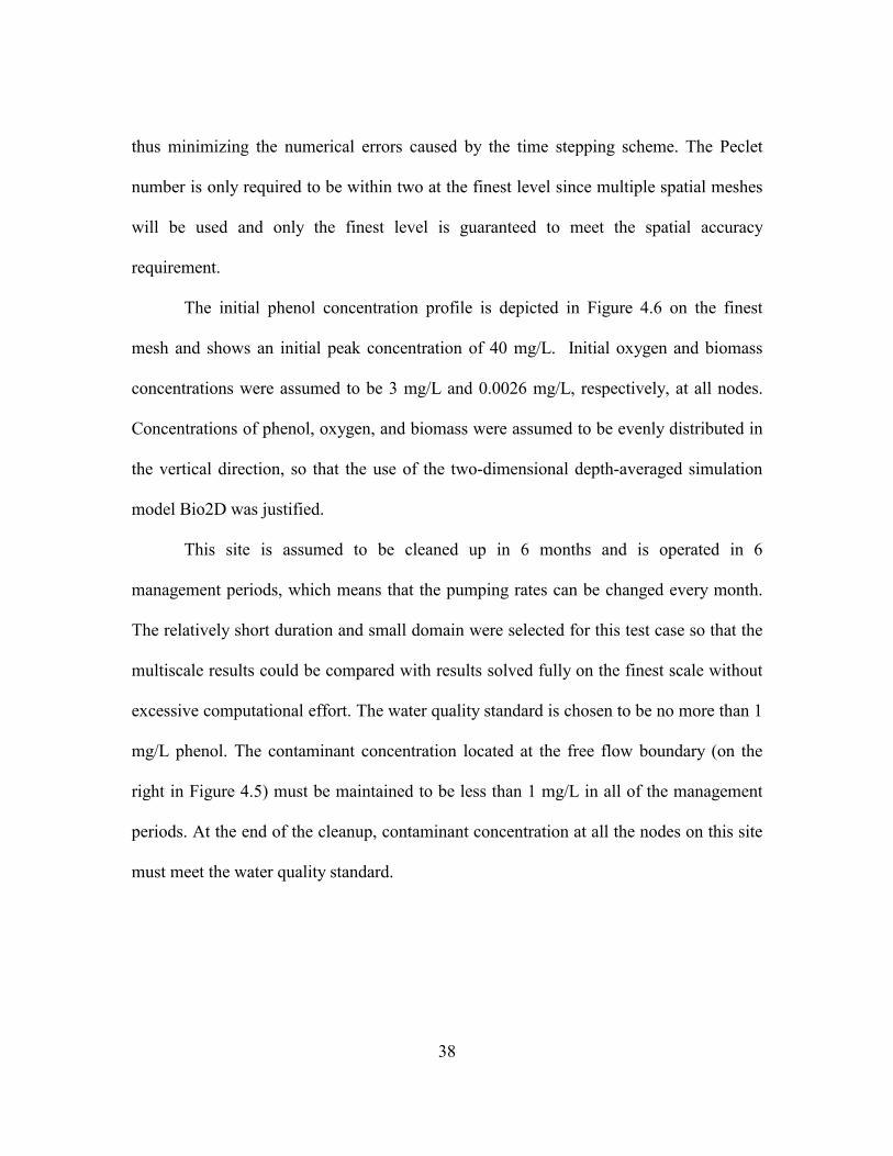
4.2.1 Description of the Test Site A plan-view schematic of the site with the coarsest mesh is shown in Figure 4.5.
The domain size is 160 m in the x-direction and 120 m in the y-direction, resulting in a
total area of 19,200 m2 . The boundary conditions are also shown in Figure 4.5. The
potential injection wells are well numbers 1-8 and the potential extraction wells are well
numbers 0 and 9.
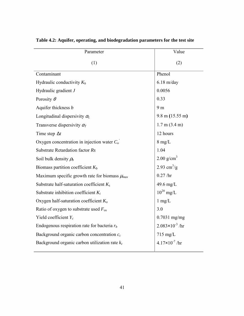
The physical parameter values for the aquifer and the site are given in Table 4.2
(hydraulic conductivity, porosity, aquifer thickness, and soil bulk density) and were taken
from Graham and McLaughlin (1991). The values of longitudinal dispersivity (αL) and
transverse dispersivity (αT) were chosen based on the recommendation by Gelhar et al.
(1992). As indicated by Gelhar et al., the reliable ratio of αL/αT is about 3 to 10 for
modeling field scale in the range of 100 m, the reliable value for αL is about 10 m, and
the reliable value for αT is around 1 m. The lower dispersivity values (αL = 9.8 m, αT =
1.7 m) in Table 4.2 were what we intended to model. However, we encountered
convergence difficulties with these values at the coarse levels, so we also considered
relatively large dispersivity values (αL = 15.55 m, αT = 3.4 m). The biological parameters
were selected for phenol and were taken from the literature (Minsker and Shoemaker
1998b). The operating parameter for oxygen concentration in the injection water is
assumed to be 8 mg/L, which is consistent with the normal dissolved oxygen
concentration in water (Minsker and Shoemaker 1998b). The time step used in the
simulation model was chosen to ensure that the Courant number is no more than one for
the range of pumping rates tested in the simulation model during the optimization run,
38
thus minimizing the numerical errors caused by the time stepping scheme. The Peclet
number is only required to be within two at the finest level since multiple spatial meshes
will be used and only the finest level is guaranteed to meet the spatial accuracy
requirement.
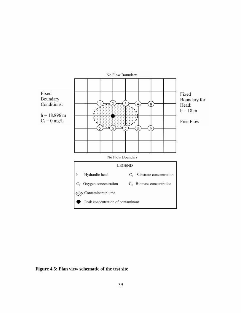
The initial phenol concentration profile is depicted in Figure 4.6 on the finest
mesh and shows an initial peak concentration of 40 mg/L. Initial oxygen and biomass
concentrations were assumed to be 3 mg/L and 0.0026 mg/L, respectively, at all nodes.
Concentrations of phenol, oxygen, and biomass were assumed to be evenly distributed in
the vertical direction, so that the use of the two-dimensional depth-averaged simulation
model Bio2D was justified.
This site is assumed to be cleaned up in 6 months and is operated in 6
management periods, which means that the pumping rates can be changed every month.
The relatively short duration and small domain were selected for this test case so that the
multiscale results could be compared with results solved fully on the finest scale without
excessive computational effort. The water quality standard is chosen to be no more than 1
mg/L phenol. The contaminant concentration located at the free flow boundary (on the
right in Figure 4.5) must be maintained to be less than 1 mg/L in all of the management
periods. At the end of the cleanup, contaminant concentration at all the nodes on this site
must meet the water quality standard.
39
2 1 3 4 0
95 6 7 8
Fixed Boundary Conditions: h = 18.896 m Cs = 0 mg/L
Fixed Boundary for Head: h = 18 m Free Flow
No Flow Boundary
No Flow Boundary
LEGEND
h Hydraulic head Cs Substrate concentration
Co Oxygen concentration Cb Biomass concentration
Contaminant plume
Peak concentration of contaminant
Figure 4.5: Plan view schematic of the test site
40
X
Y
Concentration (mg/L)
Figure 4.6: Initial contaminant plume at the test site
41
Table 4.2: Aquifer, operating, and biodegradation parameters for the test site
Parameter
(1)
Value
(2)
Contaminant Phenol
Hydraulic conductivity Kh 6.18 m/day
Hydraulic gradient J 0.0056
Porosity θ 0.33
Aquifer thickness b 9 m
Longitudinal dispersivity αL 9.8 m (15.55 m)
Transverse dispersivity αT 1.7 m (3.4 m)
Time step t∆ 12 hours
Oxygen concentration in injection water Co' 8 mg/L
Substrate Retardation factor Rs 1.04
Soil bulk density ρb 2.00 g/cm3
Biomass partition coefficient Kb 2.93 cm3/g
Maximum specific growth rate for biomass µmax 0.27 /hr
Substrate half-saturation coefficient Ks 49.6 mg/L
Substrate inhibition coefficient Ki 1020 mg/L
Oxygen half-saturation coefficient Ko 1 mg/L
Ratio of oxygen to substrate used Fos 3.0
Yield coefficient Yc 0.7031 mg/mg
Endogenous respiration rate for bacteria rb 2.083×10⁻³ /hr
Background organic carbon concentration cc 715 mg/L
Background organic carbon utilization rate kc 4.17×10⁻⁷ /hr
42
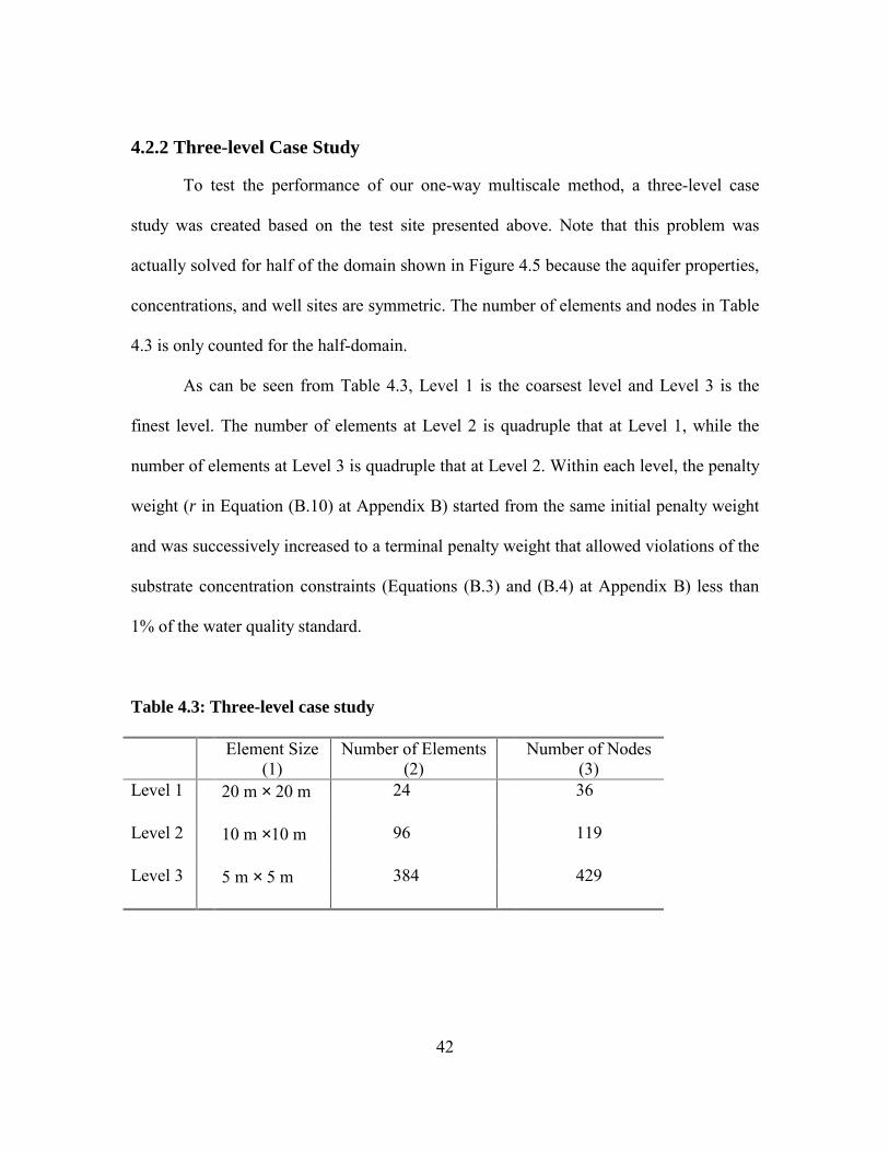
4.2.2 Three-level Case Study
To test the performance of our one-way multiscale method, a three-level case
study was created based on the test site presented above. Note that this problem was
actually solved for half of the domain shown in Figure 4.5 because the aquifer properties,
concentrations, and well sites are symmetric. The number of elements and nodes in Table
4.3 is only counted for the half-domain.
As can be seen from Table 4.3, Level 1 is the coarsest level and Level 3 is the
finest level. The number of elements at Level 2 is quadruple that at Level 1, while the
number of elements at Level 3 is quadruple that at Level 2. Within each level, the penalty
weight (r in Equation (B.10) at Appendix B) started from the same initial penalty weight
and was successively increased to a terminal penalty weight that allowed violations of the
substrate concentration constraints (Equations (B.3) and (B.4) at Appendix B) less than
1% of the water quality standard.
Table 4.3: Three-level case study
Element Size (1)
Number of Elements (2)
Number of Nodes (3)
Level 1 20 m × 20 m 24 36
Level 2 10 m ×10 m 96 119
Level 3 5 m × 5 m 384 429
43
4.3 Results and Discussions
All of the runs for the case study were conducted on an SGI Origin 2000
supercomputer using only serial code. Numerical results are discussed in the following
sections. We first discuss the results for the case with larger dispersivity values (αL =
15.55 m, αT = 3.4 m) in the first three sections and then compare them to the case with
smaller dispersivities (αL = 9.8 m, αT = 1.7 m) in the section that follows.
4.3.1 Objective Function Value vs. Iterations
The objective function value consists of the sum of the pumping costs in equation
(B.1) and the penalty value in equation (B.10) (See Appendix B). Pumping strategies that
allow water quality violations will result in adding a penalty into the objective function.
As can be seen from Figure 4.7, separate runs using the Level 1 mesh and Level 3 mesh
starting from same initial random guess result in very similar convergence behavior (in
terms of iterations). However, if we use our one-way multiscale approach to solve this
problem (i.e., the optimal pumping strategy from Level 1 mesh is used as the initial
condition on Level 2 mesh, and then the converged result on Level 2 is again used as the
initial condition on Level 3 mesh), the number of iterations needed on Level 3 is much
less than that for the standalone run on Level 3, where Level 3 is the most
computationally intensive level. A complete run of our one-way spatial multiscale
method includes 3 components, i.e., Level 1 , Level 1 to Level 2 and Level 2 to Level 3,
as plotted in all the following figures.
44
Note that the objective function value does not change significantly when
interpolating the converged result on Level 2 to Level 3 mesh, which indicates that the
optimal solution on the Level 2 mesh is a very good starting solution for the Level 3
mesh. Our later discussion explains why extra iterations were needed after the
interpolation. Also note that the significant increase in the objective function value when
interpolating the converged result on Level 1 to Level 2 results from penalties associated
with the optimal solution on the coarse mesh. After interpolation to the finer mesh, the
improvement in numerical errors results in violations of the concentration constraints.
4.3.2 Objective Function Value vs. CPU time
Figure 4.8 shows the computational savings (in terms of CPU time) associated
with solving fewer iterations on the fine mesh. It is evident from this figure that the
computing effort associated with Level 1 and Level 2 mesh solutions is much less than
that of the Level 3 mesh solution. A single run on the Level 3 mesh starting from random
initial guess needs about 117 hours, while a single run on the Level 1 mesh with the same
initial guess only needs 4.3 minutes. Using our one-way multiscale approach, however,
only about 54.5 hours are needed for the same terminal penalty weight (r = 500) to get
satisfactory results at Level 3. A terminal penalty weight refers to the last and largest
penalty weight r used in equation (B.10) (recall that r in equation (B.10) in Appendix B is
successively increased during the model solution). About 53% of the CPU time was
saved by using our one-way multiscale approach. Also note that the most CPU time
(about 98% of the total) was spent on the finest level (Level 3) for the multiscale
approach.
45
4.3.3 Maximum Violation vs. Iterations
Since we use a penalty function to convert the constrained optimization problem
to an unconstrained optimization problem, a penalty value is added to the objective
function for constraint violations. Although the objective function values change little
from Level 2 to Level 3, Figure 4.9 shows that unacceptable violations of the
concentration standards would occur if the coarser mesh solutions were used. Figure 4.9
shows the maximum (i.e., largest) violation occurring in each iteration vs. the iteration
number for the different meshes. Note that when the optimal pumping policy obtained on
the Level 1 mesh is used as an initial guess on the Level 2 mesh, a significant increase in
the maximum violation occurred. The same phenomenon was observed when
interpolating from Level 2 to Level 3, although it is not severe as from Level 1 to Level
2. This indicates that numerical errors on the Level 1 and Level 2 mesh did affect the
accuracy of the optimal solution. This also explains why 7 iterations are needed on the
finest mesh (Level 3) after interpolation to reduce the maximum violations and adjust the
optimal solution on the finest mesh to reflect the increased numerical accuracy.
4.3.4 The Impact of Low Dispersivities
In this section, we discuss the results for the case with lower dispersivity values
(αL = 9.8 m, αT = 1.7 m). We found that at Level 1 and Level 2, starting from various
random initial guesses, the case with lower dispersivity values did not converge at all.
The significant numerical errors caused by high Peclet numbers at Level 1 and Level 2
led the SALQR algorithm to choose extremely large pumping rates and diverge. To
overcome this difficulty, we modeled this case at Level 1 using artificially high
46
dispersivity values (αL = 15.55 m, αT = 3.4 m), then used the optimal results obtained at
Level 1 to interpolate to Level 2 and Level 3 using the actual lower dispersivity values.
This approach overcame the numerical difficulties caused by low dispersivity values or
high Peclet numbers. Although the converged result at Level 1 was obtained using
different and large dispersivity values, it still gave a good starting point for Level 2. Due
to the overestimation of the dispersivity values at Level 1, however, the maximum
violation after the interpolation from Level 1 to Level 2 (about 234%, see Figure 4.10) is
significantly larger than that in the previous case using the same dispersivity values at all
levels (only 49%, see Figure 4.9).
When we examine the computational savings from using our one-way spatial
multiscale approach, about 50.4% reduction in computing time at the finest level was still
achieved, as shown in Figure 4.11. Note that because of the higher dispersivity values
used at Level 1, the objective function value increased dramatically after interpolation
from Level 1 to Level 2. This is consistent with the large violations observed in Figure
4.10.
4.3.5 The Impact of Penalty Weight
During our numerical experiments, we found that, for different terminal penalty
weights used in the optimization model (r in equation (B.10) in Appendix B), the result
of interpolation was different. If a higher terminal penalty weight is used in the coarse
mesh and the converged result from the coarse mesh is used as the initial condition for
the finer mesh with the same terminal penalty weight, the number of iterations and CPU
time spent on the finer mesh will be about the same as if the model started from an initial
47
guess on the finer mesh, and the advantage of the initial solution at the coarse scale is
lost. Therefore, choosing an appropriate terminal penalty weight is a key consideration in
applying this spatial multiscale technique. Our choice of terminal penalty weight is based
on observing the maximum violations of substrate concentrations over all the monitoring
wells. If the maximum violation of substrate concentration is less than 1% of the standard
at the current penalty weight on the coarse mesh, then the penalty weight does not
increase any further. When interpolating to a finer mesh, the penalty weight is first
decreased to the same initial one used on the coarse mesh, then successively increased to
the terminal penalty weight.
To further save computing time on the finest level, which is our target solution,
we can halt the run on the finest level early before it converges with the terminal penalty
weight. Our halting criteria is that as soon as the maximum violation of substrate
concentration is less than 1% of the standard with the terminal penalty weight, we can
stop the run and accept that solution. The data presented in the above sections adopted
this halting criteria on the Level 3 mesh for both the standalone Level 3 run and the
interpolated Level 3 run.
4.4 Summary
We developed a one-way spatial multiscale method for solving an optimal control
model of in situ bioremediation of groundwater. The optimization problem is solved with
a coarse mesh initially and then the optimal strategy found with the coarse mesh is
successively interpolated to finer meshes. Initial state variables in the coarse mesh are
48
interpolated to finer meshes using a bilinear interpolation operator. Applying this
approach to a case study provided computational savings of over 50% compared with the
standalone finest mesh solution. This approach also shows advantages for modeling sites
with low dispersivities. By using relatively large dispersivities at the coarse levels and
then reducing the dispersivities at finer levels, we still achieved computational savings of
about 50%. The choice of terminal penalty weight was also shown to be critical to the
success of the spatial multiscale method. Good results were obtained when the penalty
weight was decreased after interpolation to a finer mesh and when a terminal penalty
weight was used that gave a maximum violation of the substrate concentration constraints
of less than 1% of the standard.
Our one-way spatial multiscale method shows promise for modeling larger, more
complex sites to assist in optimal in situ bioremediation design. The method is also
applicable to any other coupled simulation and optimization model in which the
simulation model can be discretized to multiple spatial scales.
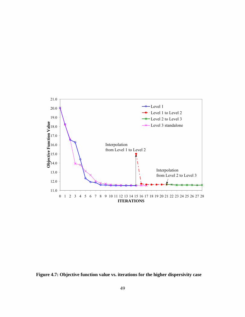
49
Figure 4.7: Objective function value vs. iterations for the higher dispersivity case
11.0
12.0
13.0
14.0
15.0
16.0
17.0
18.0
19.0
20.0
21.0
0 1 2 3 4 5 6 7 8 9 10 11 12 13 14 15 16 17 18 19 20 21 22 23 24 25 26 27 28ITERATIONS
Obj
ectiv
e Fu
nctio
n V
alue
Level 1Level 1 to Level 2Level 2 to Level 3Level 3 standalone
Interpolationfrom Level 1 to Level 2
Interpolationfrom Level 2 to Level 3
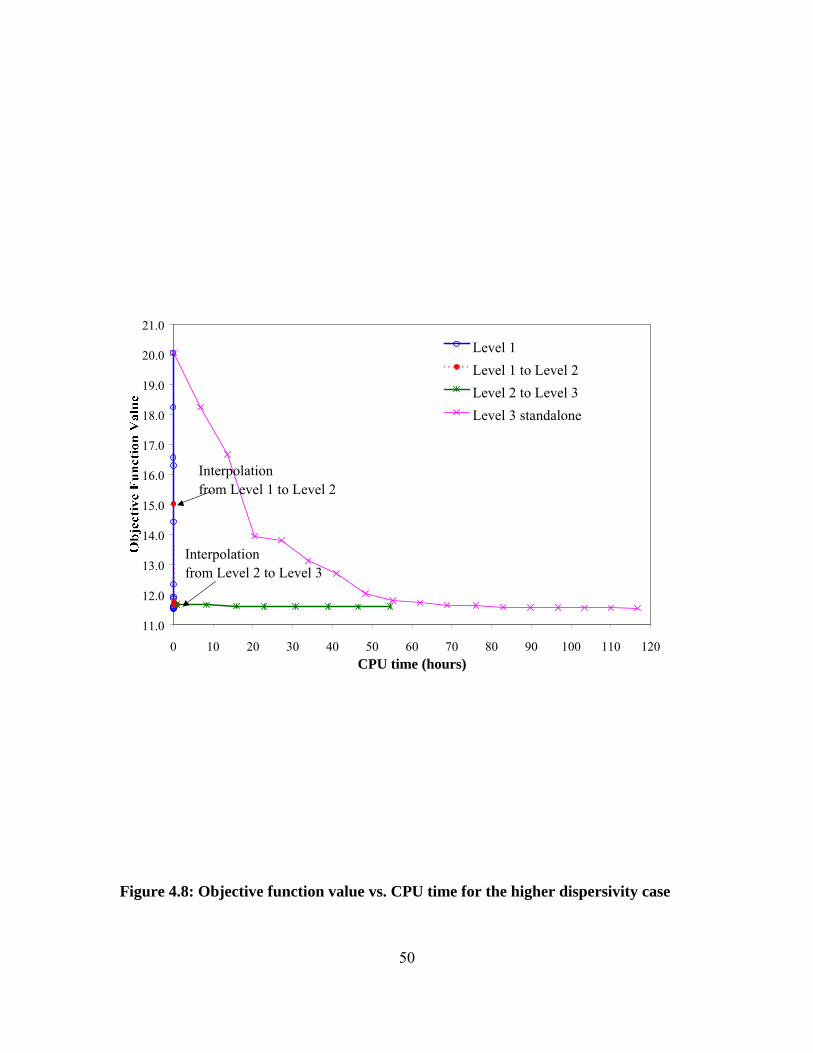
50
11.0
12.0
13.0
14.0
15.0
16.0
17.0
18.0
19.0
20.0
21.0
0 10 20 30 40 50 60 70 80 90 100 110 120CPU time (hours)
Level 1Level 1 to Level 2Level 2 to Level 3Level 3 standalone
Interpolationfrom Level 1 to Level 2
Interpolationfrom Level 2 to Level 3
Figure 4.8: Objective function value vs. CPU time for the higher dispersivity case
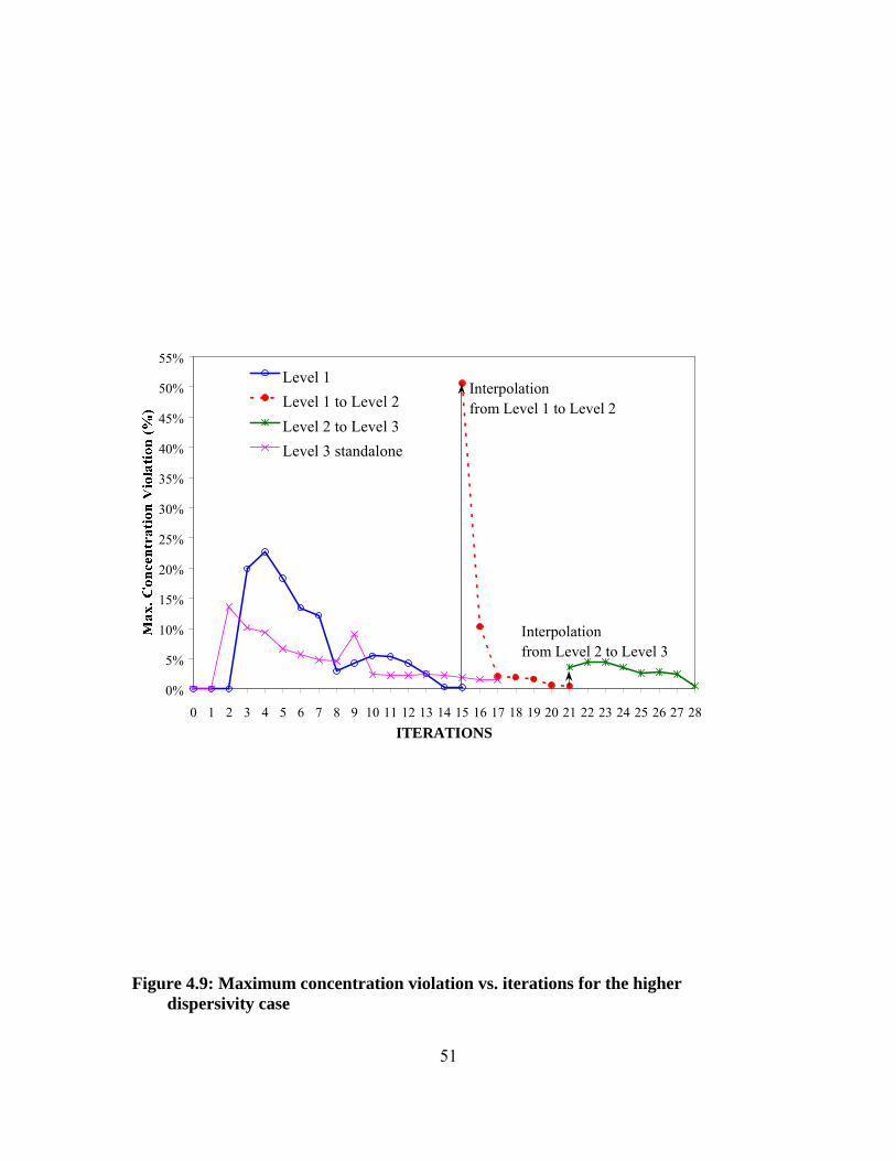
51
0%
5%
10%
15%
20%
25%
30%
35%
40%
45%
50%
55%
0 1 2 3 4 5 6 7 8 9 10 11 12 13 14 15 16 17 18 19 20 21 22 23 24 25 26 27 28ITERATIONS
Level 1Level 1 to Level 2Level 2 to Level 3Level 3 standalone
Interpolationfrom Level 1 to Level 2
Interpolationfrom Level 2 to Level 3
Figure 4.9: Maximum concentration violation vs. iterations for the higher dispersivity case
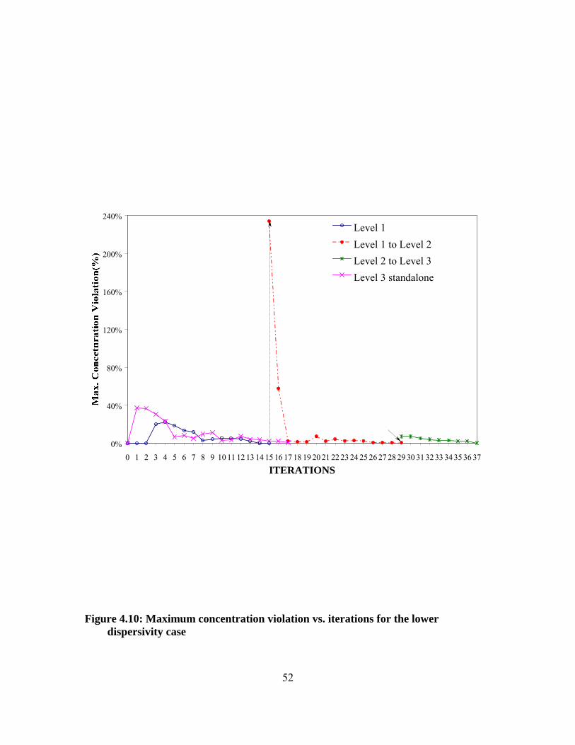
52
0%
40%
80%
120%
160%
200%
240%
0 1 2 3 4 5 6 7 8 9 10 11 12 13 14 15 16 17 18 19 20 21 22 23 24 25 26 27 28 29 30 31 32 33 34 35 36 37
ITERATIONS
Level 1Level 1 to Level 2Level 2 to Level 3Level 3 standalone
Figure 4.10: Maximum concentration violation vs. iterations for the lower dispersivity case
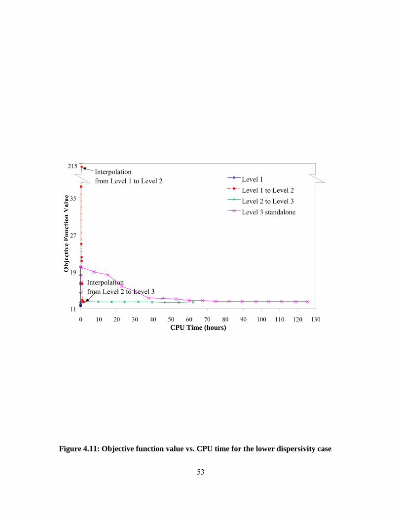
53
11
19
27
35
0 10 20 30 40 50 60 70 80 90 100 110 120 130CPU Time (hours)
Level 1Level 1 to Level 2Level 2 to Level 3Level 3 standalone
215Interpolationfrom Level 1 to Level 2
Interpolationfrom Level 2 to Level 3
Figure 4.11: Objective function value vs. CPU time for the lower dispersivity case
54
Chapter 5
Efficient Numerical Derivatives Method This chapter develops an efficient numerical derivatives method. Developing a
numerical derivatives method is necessary to implement the second spatial multiscale
method, multiscale derivatives, in the next chapter. We develop a highly efficient
implementation of one-sided forward divided difference numerical derivatives that
exploits the solution procedure for performing numerical perturbations. Both theoretical
analysis and numerical experiments are performed. Note that the one-way spatial
multiscale method developed in the last chapter is still applicable when the model uses
the efficient numerical derivatives method.
5.1 Description of the Methodology
The major concerns for implementing derivatives in an optimization model are
speed, accuracy and ease of implementation, which will be analyzed in the following
sections. Our analyses show that our numerical derivatives implementation outperforms
the previous analytical derivatives in terms of both speed and ease of implementation,
without loss of accuracy.
To understand the advantages of our numerical derivatives method, a brief review
of the previous analytical derivatives method is needed. As presented in Chapter 3, more
55
than 90% of the total CPU time for the backward sweep was used on derivative
evaluations. Moreover, the cubic growth rate of the derivatives calculation prohibits
solution of any medium- to large-scale problems with several hundred to thousands of
nodes within a reasonable time period. Furthermore, the analytical derivatives have to be
re-derived each time the simulation model changes, limiting flexibility of the
management model. Thus, this approach is human-labor intensive and impractical for
complex two- or three-dimensional simulation models.
Despite the above limitations, it is commonly held that analytical derivatives
usually provide better accuracy and faster computing times once coded. Whiffen (1995)
showed that one-sided divided difference approximations of the derivatives took 29 times
the CPU time required to compute analytical derivatives in his SALQR model. Although
the implementation details of Whiffens numerical derivatives were not given, the general
belief that numerical derivatives are slower than analytical derivatives is not necessarily
true, as will be demonstrated below.
A one-sided divided difference approximation of the derivatives ∂Y/ ∂X and
∂Y/∂U at each management period can be formulated as follows:
kNNik XY
XY
XY
XY
XY
XY
∂∂
∂∂
∂∂
∂∂
∂∂=
∂∂
−121
LL (5.1)
kmmjk XY
UY
UY
UY
UY
UY
∂∂
∂∂
∂∂
∂∂
∂∂=
∂∂
−121
LL (5.2)
ii XXoldXnew
XY
∆−=
∂∂ , i = 1,… N (5.3)
jj UXoldXnew
UY
∆−=
∂∂ , j = 1, … m (5.4)
56
where Xnew and Xold are the state vectors before and after the perturbation respectively,
which both have a dimension of N, where N is the total number of non-Dirichlet state
variables; subscript i and j are the ith state variable or jth control variable in the state
vector or control vector; and the subscript k stands for the management period counter.
The dimension of ∂Y/∂Xi is a column vector of length N. The dimension of ∂Y/∂Uj is a
column vector of length m, where m is the total number of control variables. Each of the k
matrices ∂Y/∂X has dimension N by N and is composed of N vectors of ∂Y/ ∂Xi for the kth
management period. Correspondingly, each matrix ∂Y/∂U has dimension N by m and is
composed of m vectors of ∂Y/∂Uj for the kth management period. Since the pumping rates
(control vector U) change only at each management period, ∂Y/∂X and ∂Y/∂U are only
calculated once at each management period k by direct perturbation in one step. This is in
contrast to the previous analytical derivatives method, where management period
derivatives can only be obtained at the second step after the simulation time step
derivatives have been calculated. In the numerical derivatives method, each perturbation
requires one run of the simulation model from the beginning of one management period
to the end of that management period.
Efficiency of the implementation described previously depends on how the
simulation model is run under the perturbation. The most obvious implementation would
require re-solving the simulation model without using any information available in the
forward sweep of the algorithm, which would certainly be inferior to the analytical
derivatives method. The efficient implementation of numerical derivatives presented
57
herein is based on the observation that, when calculating the first derivatives of the
transition equation with respect to the state variables, small perturbations of a single state
variable only affect the right-hand-side of the resulting linear system of equations
describing the transition equation (after all, running any numerical groundwater fate and
transport model can eventually be reduced to solving a linear system of equations). Thus,
saving the results of the previous forward sweep and the LU factorization results of the
left-hand-side matrix, where the simulation model is run normally, benefits the
perturbation run of the simulation model since only the right-hand-side of the system
equation need be reformulated and backward substitution applied to obtain the simulation
results under the perturbation. This method is general in that it is independent of the
simulation model (i.e., remediation technology) used and is much easier to implement
than the previous analytical derivatives method. Detailed implementation of this method
for the optimal control model of groundwater bioremediation is presented subsequently.
Note that only the implementation for the state vector derivatives (∂Y/∂X) is presented.
The control vector derivatives (∂Y/∂U) must be calculated using the standard method of
solving the entire simulation model for each perturbation since each perturbation affects
the left-hand-side of the transition equation. However, given that the dimension of the
control vector is usually much smaller than the state vector, computational effort is most
often driven by the state vector derivatives calculation.
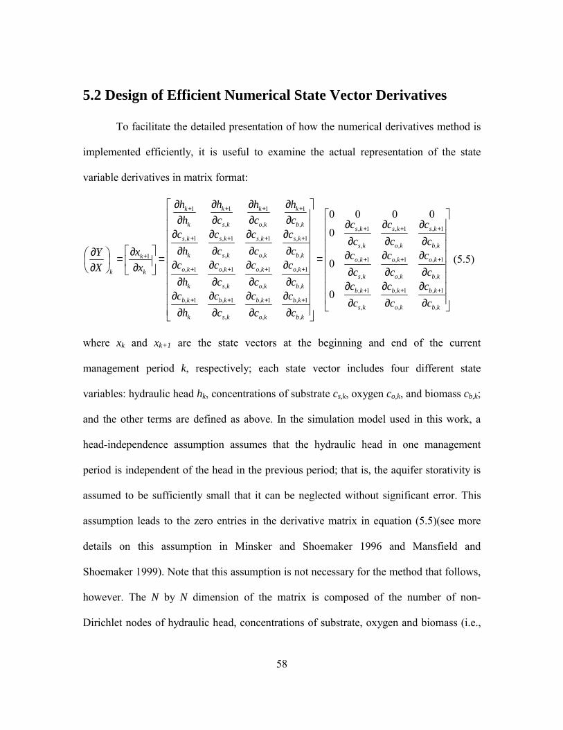
58
5.2 Design of Efficient Numerical State Vector Derivatives
To facilitate the detailed presentation of how the numerical derivatives method is
implemented efficiently, it is useful to examine the actual representation of the state
variable derivatives in matrix format:
∂∂
∂∂
∂∂
∂∂
∂∂
∂∂
∂∂
∂∂
∂∂
=
∂∂
∂∂
∂∂
∂∂
∂∂
∂∂
∂∂
∂∂
∂∂
∂∂
∂∂
∂∂
∂∂
∂∂
∂∂
∂∂
=
∂∂=
∂∂
+++
+++
+++
++++
++++
++++
++++
+
kb
kb
ko
kb
ks
kb
kb
ko
ko
ko
ks
ko
kb
ks
ko
ks
ks
ks
kb
kb
ko
kb
ks
kb
k
kb
kb
ko
ko
ko
ks
ko
k
ko
kb
ks
ko
ks
ks
ks
k
ks
kb
k
ko
k
ks
k
k
k
k
k
k
cc
cc
cc
cc
cc
cc
cc
cc
cc
cc
cc
cc
hc
cc
cc
cc
hc
cc
cc
cc
hc
ch
ch
ch
hh
xx
XY
,
1,
,
1,
,
1,
,
1,
,
1,
,
1,
,
1,
,
1,
,
1,
,
1,
,
1,
,
1,1,
,
1,
,
1,
,
1,1,
,
1,
,
1,
,
1,1,
,
1
,
1
,
11
1
0
0
0
0000
(5.5)
where xk and xk+1 are the state vectors at the beginning and end of the current
management period k, respectively; each state vector includes four different state
variables: hydraulic head hk, concentrations of substrate cs,k, oxygen co,k, and biomass cb,k;
and the other terms are defined as above. In the simulation model used in this work, a
head-independence assumption assumes that the hydraulic head in one management
period is independent of the head in the previous period; that is, the aquifer storativity is
assumed to be sufficiently small that it can be neglected without significant error. This
assumption leads to the zero entries in the derivative matrix in equation (5.5)(see more
details on this assumption in Minsker and Shoemaker 1996 and Mansfield and
Shoemaker 1999). Note that this assumption is not necessary for the method that follows,
however. The N by N dimension of the matrix is composed of the number of non-
Dirichlet nodes of hydraulic head, concentrations of substrate, oxygen and biomass (i.e.,
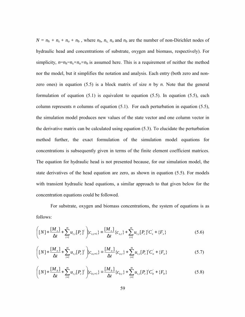
59
N = nh + ns + no + nb , where nh, ns, no and nb are the number of non-Dirichlet nodes of
hydraulic head and concentrations of substrate, oxygen and biomass, respectively). For
simplicity, n=nh=ns=no=nb is assumed here. This is a requirement of neither the method
nor the model, but it simplifies the notation and analysis. Each entry (both zero and non-
zero ones) in equation (5.5) is a block matrix of size n by n. Note that the general
formulation of equation (5.1) is equivalent to equation (5.5). In equation (5.5), each
column represents n columns of equation (5.1). For each perturbation in equation (5.5),
the simulation model produces new values of the state vector and one column vector in
the derivative matrix can be calculated using equation (5.3). To elucidate the perturbation
method further, the exact formulation of the simulation model equations for
concentrations is subsequently given in terms of the finite element coefficient matrices.
The equation for hydraulic head is not presented because, for our simulation model, the
state derivatives of the head equation are zero, as shown in equation (5.5). For models
with transient hydraulic head equations, a similar approach to that given below for the
concentration equations could be followed.
For substrate, oxygen and biomass concentrations, the system of equations is as
follows:
][][][][][ '
1,,1,
1, ss
m
i
icitts
sts
m
i
icit
s FCPuct
McPut
MN ++∆
=
+∆
+ ∑∑=
+=
(5.6)
][][][][][ '
1,,1,
1, oo
m
i
icitto
oto
m
i
icit
o FCPuct
McPut
MN ++∆
=
+∆
+ ∑∑=
+=
(5.7)
][][][][][ '
1,,1,
1, bb
m
i
icittb
btb
m
i
icit
b FCPuct
McPut
MN ++∆
=
+∆
+ ∑∑=
+=
(5.8)
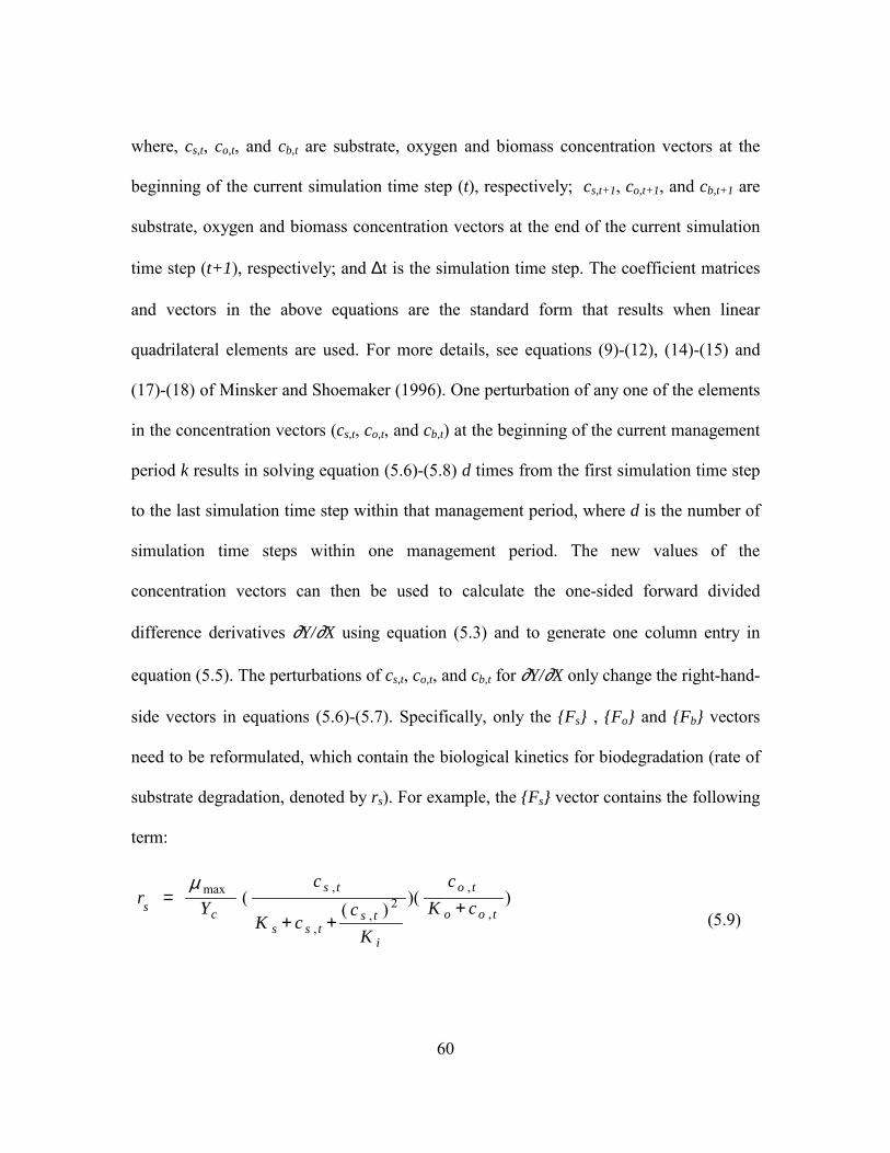
60
where, cs,t, co,t, and cb,t are substrate, oxygen and biomass concentration vectors at the
beginning of the current simulation time step (t), respectively; cs,t+1, co,t+1, and cb,t+1 are
substrate, oxygen and biomass concentration vectors at the end of the current simulation
time step (t+1), respectively; and ∆t is the simulation time step. The coefficient matrices
and vectors in the above equations are the standard form that results when linear
quadrilateral elements are used. For more details, see equations (9)-(12), (14)-(15) and
(17)-(18) of Minsker and Shoemaker (1996). One perturbation of any one of the elements
in the concentration vectors (cs,t, co,t, and cb,t) at the beginning of the current management
period k results in solving equation (5.6)-(5.8) d times from the first simulation time step
to the last simulation time step within that management period, where d is the number of
simulation time steps within one management period. The new values of the
concentration vectors can then be used to calculate the one-sided forward divided
difference derivatives ∂Y/∂X using equation (5.3) and to generate one column entry in
equation (5.5). The perturbations of cs,t, co,t, and cb,t for ∂Y/∂X only change the right-hand-
side vectors in equations (5.6)-(5.7). Specifically, only the Fs , Fo and Fb vectors
need to be reformulated, which contain the biological kinetics for biodegradation (rate of
substrate degradation, denoted by rs). For example, the Fs vector contains the following
term:
))()(
(,
,2
,,
,max
too
to
i
tstss
ts
cs cKc
Kc
cK
cYr +
++=
µ
(5.9)
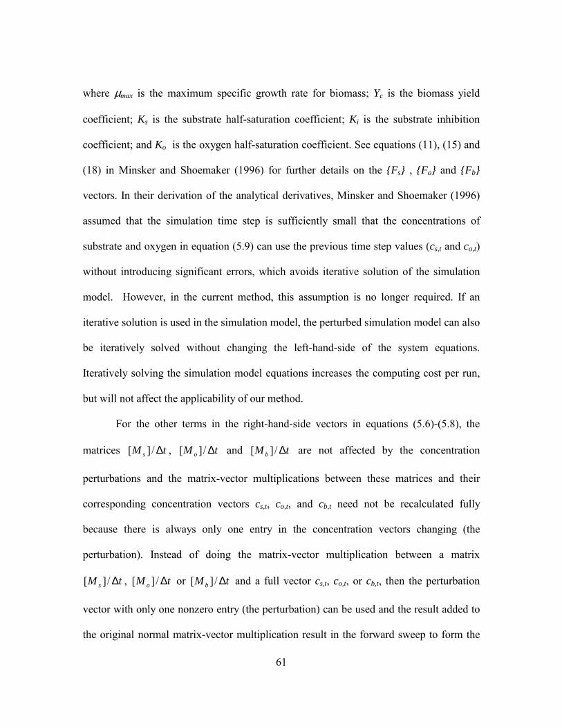
61
where µmax is the maximum specific growth rate for biomass; Yc is the biomass yield
coefficient; Ks is the substrate half-saturation coefficient; Ki is the substrate inhibition
coefficient; and Ko is the oxygen half-saturation coefficient. See equations (11), (15) and
(18) in Minsker and Shoemaker (1996) for further details on the Fs , Fo and Fb
vectors. In their derivation of the analytical derivatives, Minsker and Shoemaker (1996)
assumed that the simulation time step is sufficiently small that the concentrations of
substrate and oxygen in equation (5.9) can use the previous time step values (cs,t and co,t)
without introducing significant errors, which avoids iterative solution of the simulation
model. However, in the current method, this assumption is no longer required. If an
iterative solution is used in the simulation model, the perturbed simulation model can also
be iteratively solved without changing the left-hand-side of the system equations.
Iteratively solving the simulation model equations increases the computing cost per run,
but will not affect the applicability of our method.
For the other terms in the right-hand-side vectors in equations (5.6)-(5.8), the
matrices tM s ∆/][ , tM o ∆/][ and tM b ∆/][ are not affected by the concentration
perturbations and the matrix-vector multiplications between these matrices and their
corresponding concentration vectors cs,t, co,t, and cb,t need not be recalculated fully
because there is always only one entry in the concentration vectors changing (the
perturbation). Instead of doing the matrix-vector multiplication between a matrix
tM s ∆/][ , tM o ∆/][ or tM b ∆/][ and a full vector cs,t, co,t, or cb,t, then the perturbation
vector with only one nonzero entry (the perturbation) can be used and the result added to
the original normal matrix-vector multiplication result in the forward sweep to form the
62
first terms in equations (5.6)-(5.8). The computational effort for obtaining this term thus
reduces to O(N) from O(N2). The pumping source term '
1, ][ CPu
m
i
icit∑
=
is constant with
respect to concentrations (C’ represents the injection concentration, which is assumed to
be constant).
In summary, calculating the derivative matrices of equation (5.5) by perturbing
concentrations in (5.6)-(5.8) only changes the right-hand-side of each equation relative to
the runs in the forward sweep. This result occurs because only the right-hand-side vector
is affected by perturbations in the initial state variables at the beginning of the
management period, the importance of which is explained subsequently. Note that in
performing the perturbations, perturbation increments of 0.01% for substrate and oxygen
and 0.0001% for biomass concentrations were found to produce sufficiently accurate
numerical derivatives. Of course, the appropriate perturbation increment may vary for
different applications.
5.3 Theoretical Analysis of the Computational Effort
Associated with the Numerical Derivatives Method
Given that each perturbation to obtain equation (5.5) can be obtained by
reformulating the right-hand-side vectors and performing back substitution, the
theoretical computing effort for running the perturbed simulation model is on the order of
O(N), where N is the number of non-Dirichlet state variables. Thus, calculating derivative
63
∂Y/∂X using the one-sided divided difference method with N perturbations is only O(N2).
This is an order of magnitude reduction in the computing time compared to the previous
analytical derivatives method, which is O(N3), as we analyzed at the beginning of this
section. Calculating the first derivatives of the transition equation with respect to the
control variables (∂Y/∂U), which, as mentioned earlier, requires re-solving the whole
simulation model, entails O(m(s+1)2N) work, where s is the bandwidth (e.g., for a tri-
diagonal matrix, s=1; see the definition in Iserles, 1996) and m is the total number of
control variables. Since the number of control variables (i.e. pumping wells) is usually far
less than the number of nodes in the finite element mesh, the number of runs of the full
simulation model for ∂Y/∂U contributes less to the total computing time. In the actual
implementation of this method, the growth rate will be slightly higher than quadratic due
to the calculation of ∂Y/∂U and storage of the results of the forward sweep run.
5.4 Case Study
5.4.1 Description of the Test Case
To test the performance of our numerical derivatives method, a four-level case study
was created based on the test site presented in Chapter 4. A scenario with dispersivity
values of αL = 15.55 m and αT = 3.4 m was used in this analysis. Note that this problem
was actually solved for half of the domain shown in Figure 4.5 because the aquifer
properties, concentrations, and well sites are symmetric. The number of elements and
nodes in Table 5.1 is only counted for the half-domain. Note that the number of non-
Dirichlet state variables is four times the number of numerical nodes if the dimensions of
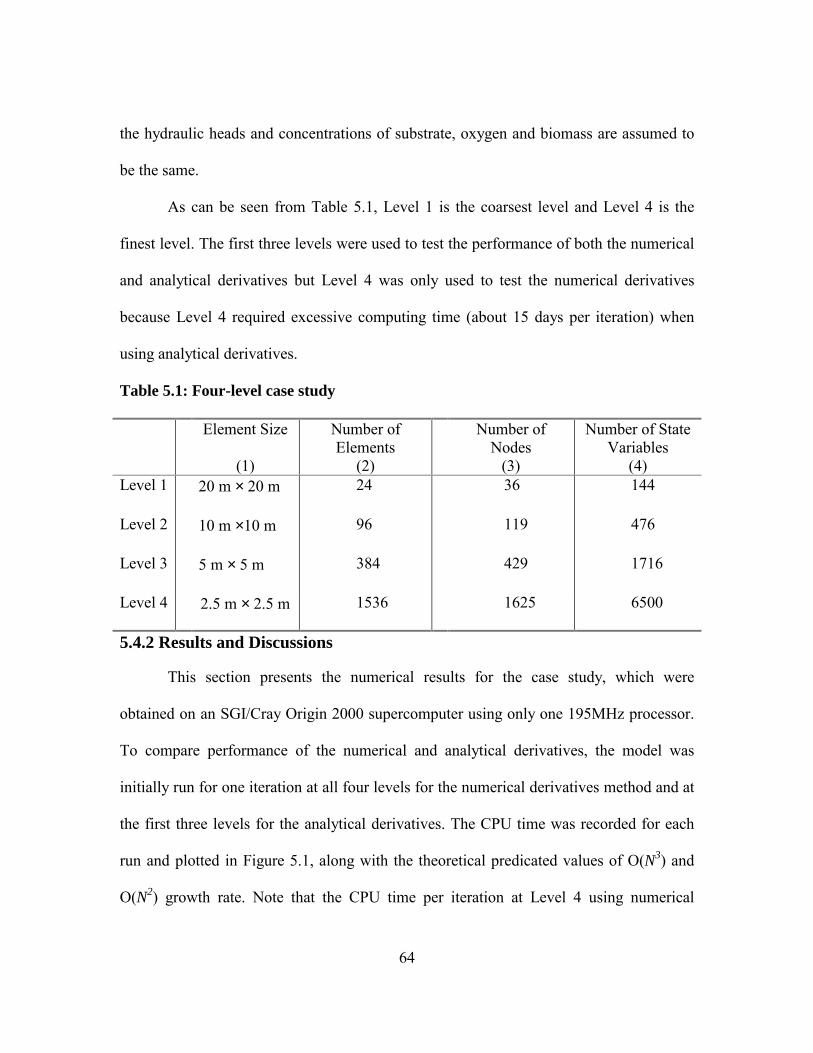
64
the hydraulic heads and concentrations of substrate, oxygen and biomass are assumed to
be the same.
As can be seen from Table 5.1, Level 1 is the coarsest level and Level 4 is the
finest level. The first three levels were used to test the performance of both the numerical
and analytical derivatives but Level 4 was only used to test the numerical derivatives
because Level 4 required excessive computing time (about 15 days per iteration) when
using analytical derivatives.
Table 5.1: Four-level case study
Element Size
(1)
Number of Elements
(2)
Number of Nodes
(3)
Number of State Variables
(4) Level 1 20 m × 20 m 24 36 144
Level 2 10 m ×10 m 96 119 476
Level 3 5 m × 5 m 384 429 1716
Level 4 2.5 m × 2.5 m 1536 1625 6500
5.4.2 Results and Discussions
This section presents the numerical results for the case study, which were
obtained on an SGI/Cray Origin 2000 supercomputer using only one 195MHz processor.
To compare performance of the numerical and analytical derivatives, the model was
initially run for one iteration at all four levels for the numerical derivatives method and at
the first three levels for the analytical derivatives. The CPU time was recorded for each
run and plotted in Figure 5.1, along with the theoretical predicated values of O(N3) and
O(N2) growth rate. Note that the CPU time per iteration at Level 4 using numerical
65
derivatives is approximately 2.3 days and the estimated CPU time per iteration at Level 4
using analytical derivatives is about 15 days, which were off the scale and are hence not
shown.
As can be seen from Figure 5.1, the CPU time per iteration using analytical
derivatives grows dramatically with the increase in level number as the number of state
variables increases (as predicted in Table 4.1). Based on the measured CPU times per
iteration using analytical derivatives, the growth rate can be fit and the result is O(N2.97),
which is very close to the theoretical prediction O(N3) of the SALQR model (Liao and
Shoemaker, 1991). In contrast, the CPU time per iteration using numerical derivatives
implemented in this study has a much lower growth rate. Based on the measured CPU
times per iteration using numerical derivatives, the growth rate can be calculated and
denoted as O(N2.18), which is close to the prediction calculated in the methodology
section. This is a significant improvement over the previous analytical derivatives
method. The lower order growth rate implies that as the number of state variables
increases, more and more computational savings can be obtained using our numerical
derivatives method over analytical derivatives. Although at Level 1 the analytical method
was actually slightly faster than the numerical method presented herein, as the grid size
increased the analytical method became much slower than the numerical method. For
realistically sized optimal control problems, it is expected that the numerical method will
be substantially faster than the analytical method.
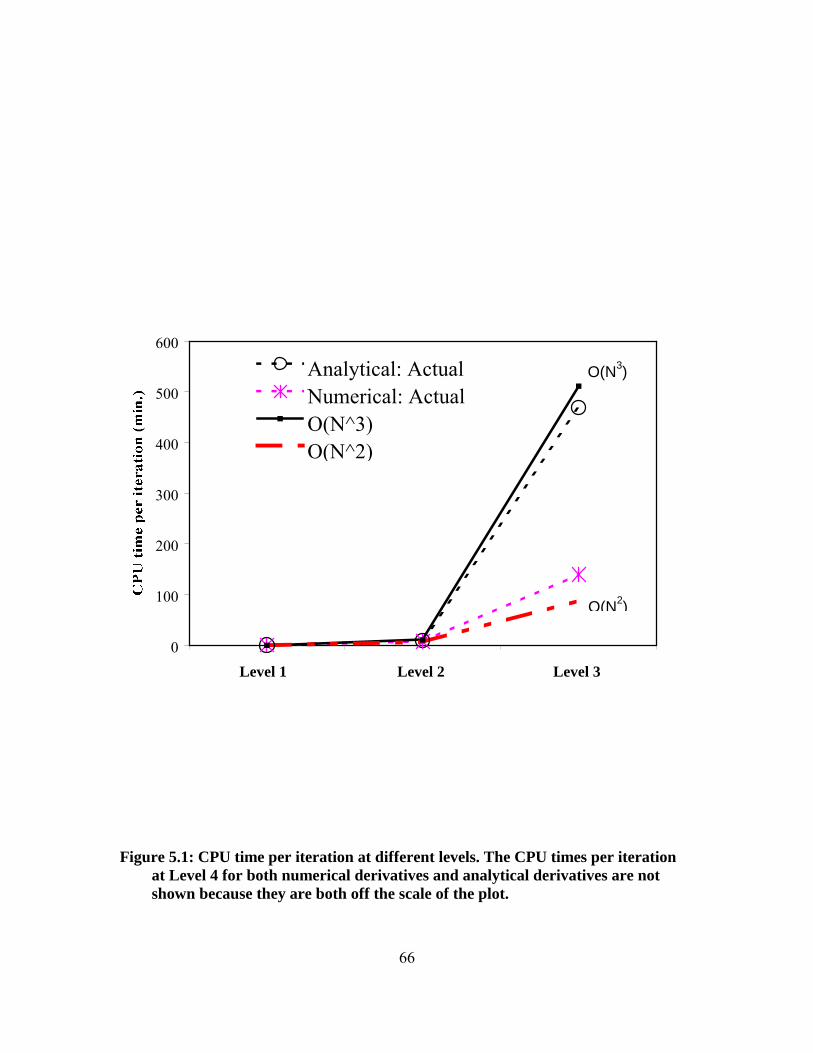
66
0
100
200
300
400
500
600
Level 1 Level 2 Level 3
Analytical: ActualNumerical: ActualO(N^3)O(N^2)
O(N3)
O(N2)
Figure 5.1: CPU time per iteration at different levels. The CPU times per iteration
at Level 4 for both numerical derivatives and analytical derivatives are not shown because they are both off the scale of the plot.
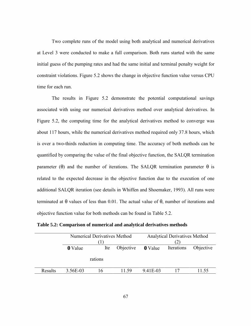
67
Two complete runs of the model using both analytical and numerical derivatives
at Level 3 were conducted to make a full comparison. Both runs started with the same
initial guess of the pumping rates and had the same initial and terminal penalty weight for
constraint violations. Figure 5.2 shows the change in objective function value versus CPU
time for each run.
The results in Figure 5.2 demonstrate the potential computational savings
associated with using our numerical derivatives method over analytical derivatives. In
Figure 5.2, the computing time for the analytical derivatives method to converge was
about 117 hours, while the numerical derivatives method required only 37.8 hours, which
is over a two-thirds reduction in computing time. The accuracy of both methods can be
quantified by comparing the value of the final objective function, the SALQR termination
parameter (θ) and the number of iterations. The SALQR termination parameter θ is
related to the expected decrease in the objective function due to the execution of one
additional SALQR iteration (see details in Whiffen and Shoemaker, 1993). All runs were
terminated at θ values of less than 0.01. The actual value of θ, number of iterations and
objective function value for both methods can be found in Table 5.2.
Table 5.2: Comparison of numerical and analytical derivatives methods
Numerical Derivatives Method (1)
Analytical Derivatives Method (2)
θθθθ Value Ite
rations
Objective θθθθ Value Iterations Objective
Results 3.56E-03 16 11.59 9.41E-03 17 11.55
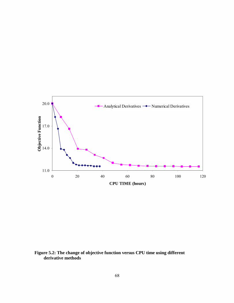
68
11.0
14.0
17.0
20.0
0 20 40 60 80 100 120
CPU TIME (hours)
Obj
ectiv
e Fu
nctio
n
Analytical Derivatives Numerical Derivatives
Figure 5.2: The change of objective function versus CPU time using different
derivative methods
69
As shown in Table 5.2, values of θ for both the numerical and analytical
derivatives methods were less than the required termination value of 0.01, which means
that all runs successfully terminated. Moreover, there is no practical difference in the
final objective function value. The number of iterations using the numerical derivatives
method was less than that using the analytical derivatives method, indicating that
accuracy does not deteriorate using the numerical derivatives method. In fact, the
numerical derivatives may even be more accurate because the management period
derivatives are directly calculated. In the analytical derivatives method, the management
period derivatives are the product of 60 simulation period derivative matrices since each
management period consists of 60 simulation time steps. When the matrices contain
numerous small floating-point numbers of different scales, these multiplications can
cause significant numerical rounding errors (Minsker and Shoemaker, 1998a).
Note that both derivatives methods identified solutions with nearly identical cost
(In fact, the costs only differ by 0.4%) but the pumping rates were somewhat different.
The optimal pumping rates obtained by both derivatives methods can be found in Figures
5.3 to 5.8. Since there are 6 management periods in this case study, for each well
location, there is a change in pumping rates in each management period. It is very
interesting that for the first 3 management periods, the pumping rates and patterns are
almost the same for both methods. However, in the last three management periods,
different pumping patterns are found to be optimal. The injection wells reach minimum
pumping rates in management period 5 for the solution obtained from the numerical
derivatives method, while the analytical derivatives method produces a solution whose
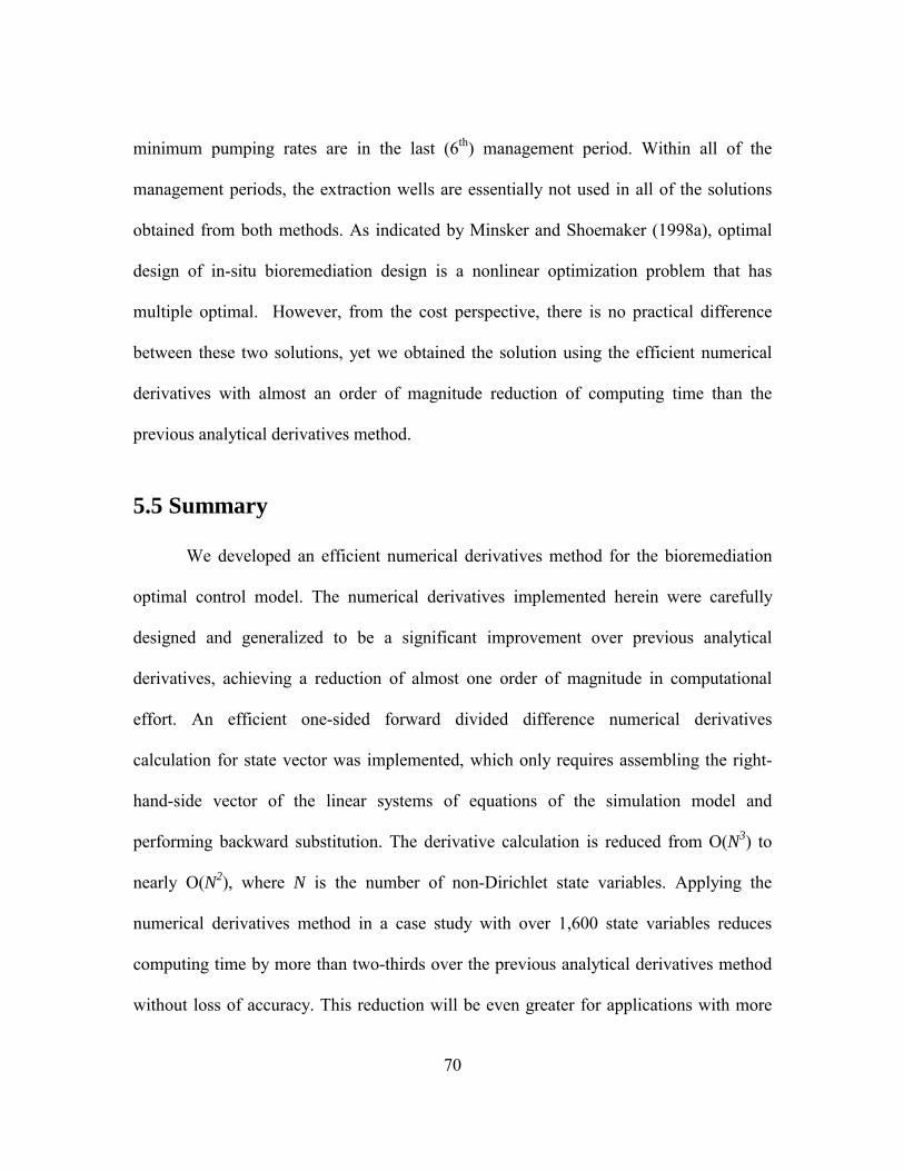
70
minimum pumping rates are in the last (6th) management period. Within all of the
management periods, the extraction wells are essentially not used in all of the solutions
obtained from both methods. As indicated by Minsker and Shoemaker (1998a), optimal
design of in-situ bioremediation design is a nonlinear optimization problem that has
multiple optimal. However, from the cost perspective, there is no practical difference
between these two solutions, yet we obtained the solution using the efficient numerical
derivatives with almost an order of magnitude reduction of computing time than the
previous analytical derivatives method.
5.5 Summary
We developed an efficient numerical derivatives method for the bioremediation
optimal control model. The numerical derivatives implemented herein were carefully
designed and generalized to be a significant improvement over previous analytical
derivatives, achieving a reduction of almost one order of magnitude in computational
effort. An efficient one-sided forward divided difference numerical derivatives
calculation for state vector was implemented, which only requires assembling the right-
hand-side vector of the linear systems of equations of the simulation model and
performing backward substitution. The derivative calculation is reduced from O(N3) to
nearly O(N2), where N is the number of non-Dirichlet state variables. Applying the
numerical derivatives method in a case study with over 1,600 state variables reduces
computing time by more than two-thirds over the previous analytical derivatives method
without loss of accuracy. This reduction will be even greater for applications with more
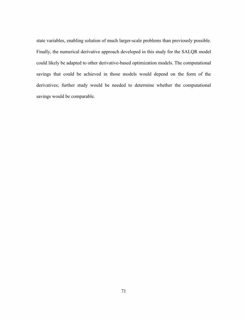
71
state variables, enabling solution of much larger-scale problems than previously possible.
Finally, the numerical derivative approach developed in this study for the SALQR model
could likely be adapted to other derivative-based optimization models. The computational
savings that could be achieved in those models would depend on the form of the
derivatives; further study would be needed to determine whether the computational
savings would be comparable.
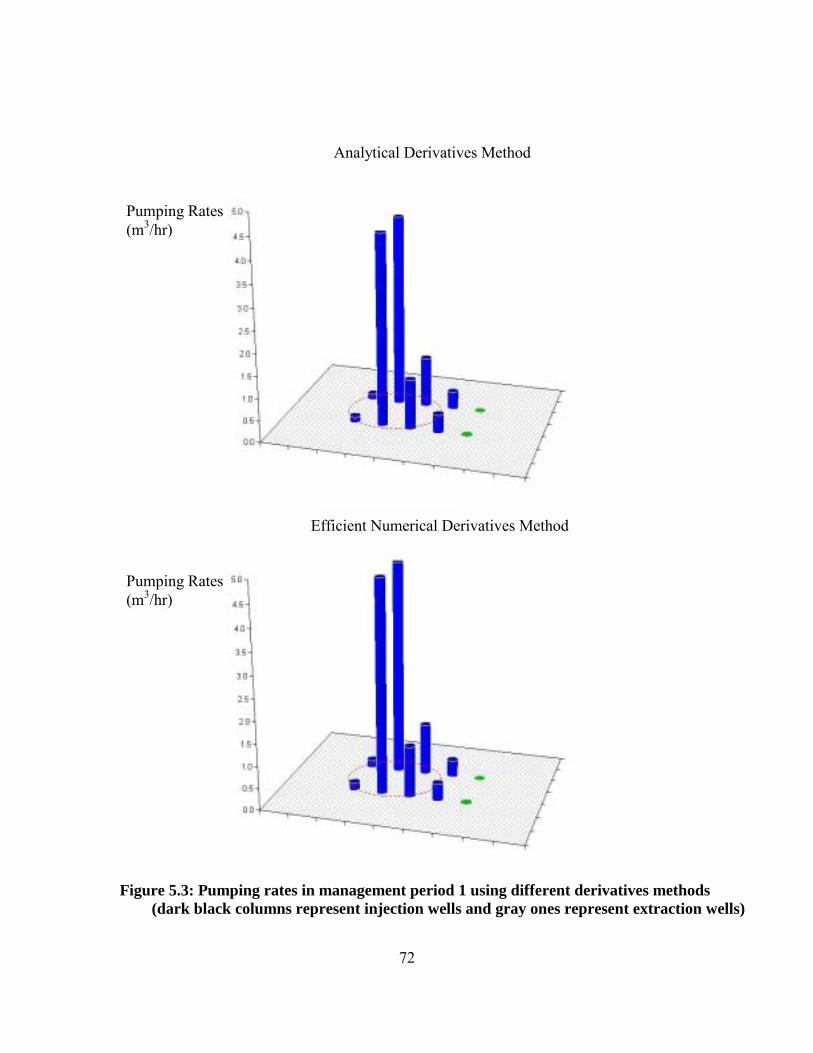
72
Figure 5.3: Pumping rates in management period 1 using different derivatives methods (dark black columns represent injection wells and gray ones represent extraction wells)
Analytical Derivatives Method
Efficient Numerical Derivatives Method
Pumping Rates (m3/hr)
Pumping Rates (m3/hr)
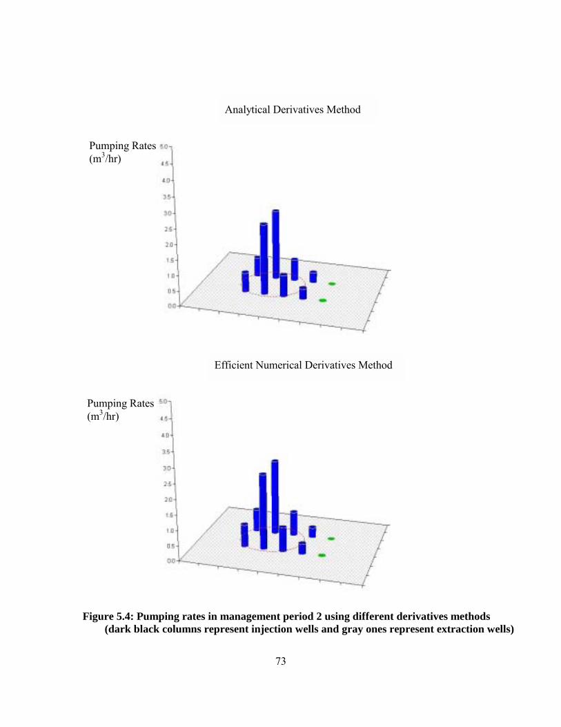
73
Figure 5.4: Pumping rates in management period 2 using different derivatives methods (dark black columns represent injection wells and gray ones represent extraction wells)
Analytical Derivatives Method Analytical Derivatives Method
Efficient Numerical Derivatives Method
Pumping Rates (m3/hr)
Pumping Rates (m3/hr)
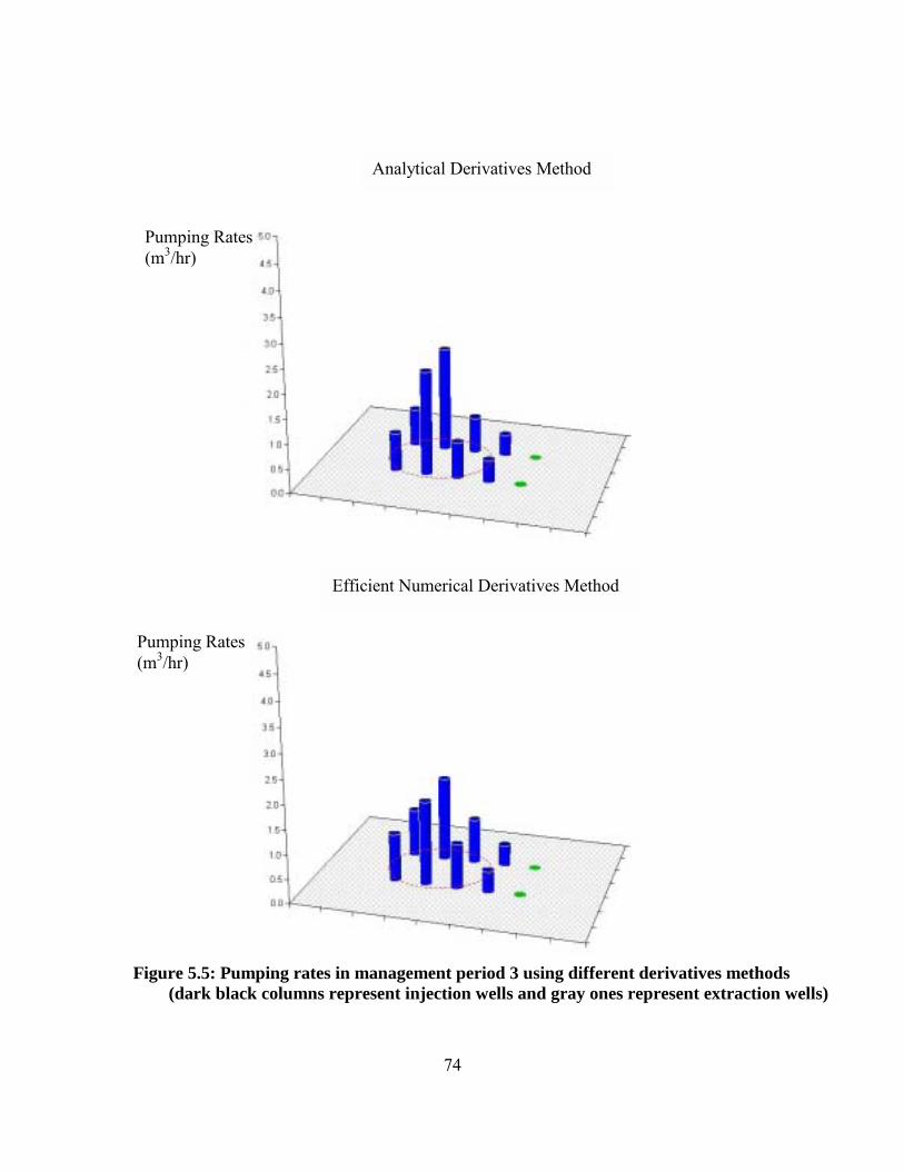
74
Figure 5.5: Pumping rates in management period 3 using different derivatives methods
(dark black columns represent injection wells and gray ones represent extraction wells)
Analytical Derivatives Method
Efficient Numerical Derivatives Method
Pumping Rates (m3/hr)
Pumping Rates (m3/hr)
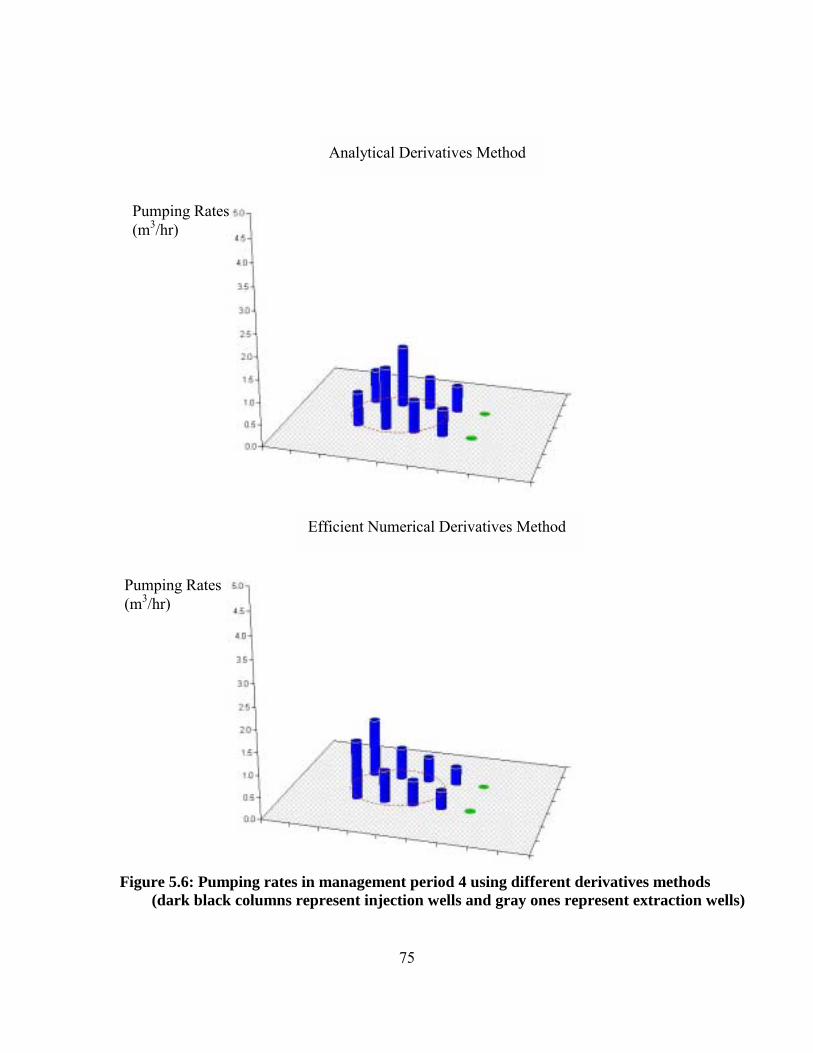
75
Figure 5.6: Pumping rates in management period 4 using different derivatives methods
(dark black columns represent injection wells and gray ones represent extraction wells)
Analytical Derivatives Method
Efficient Numerical Derivatives Method
Pumping Rates (m3/hr)
Pumping Rates (m3/hr)
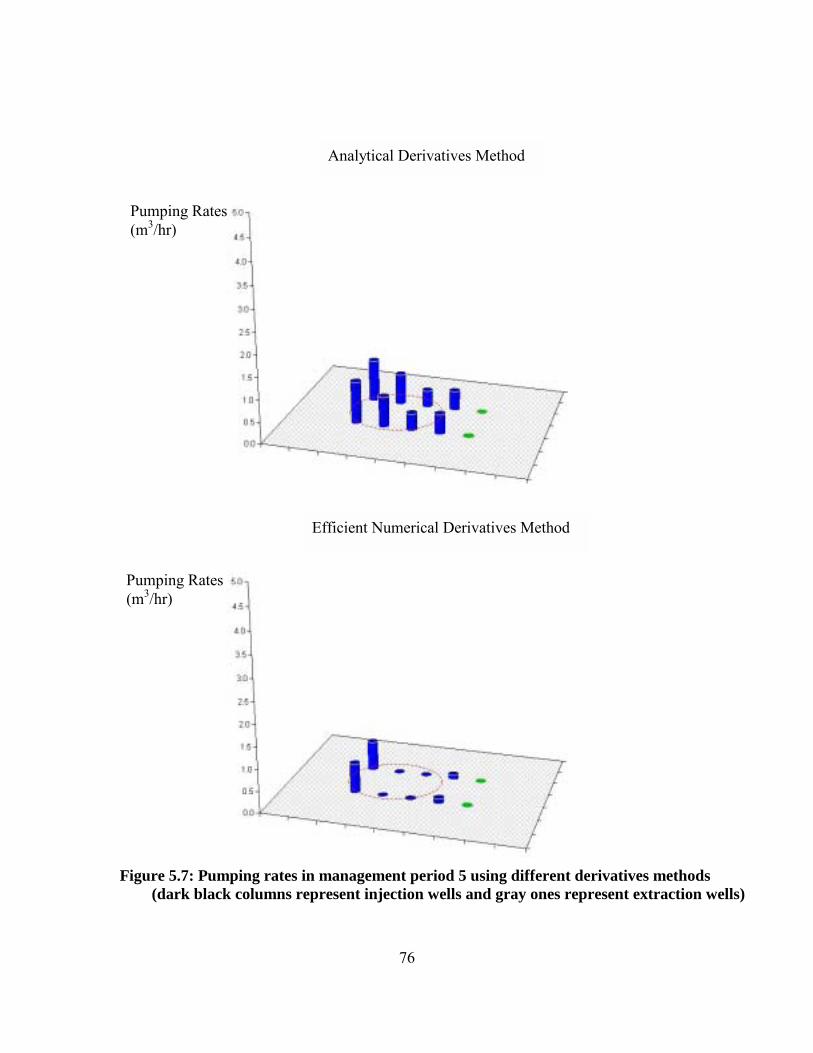
76
Figure 5.7: Pumping rates in management period 5 using different derivatives methods
(dark black columns represent injection wells and gray ones represent extraction wells)
Analytical Derivatives Method
Efficient Numerical Derivatives Method
Pumping Rates (m3/hr)
Pumping Rates (m3/hr)
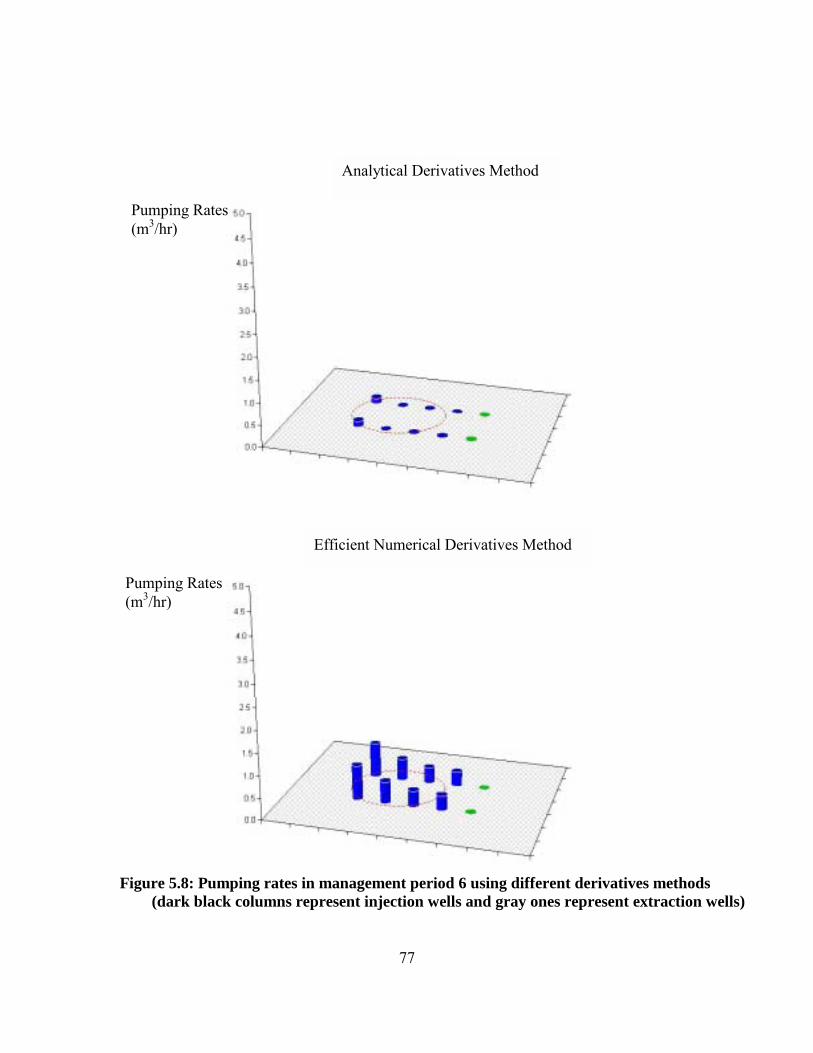
77
Figure 5.8: Pumping rates in management period 6 using different derivatives methods
(dark black columns represent injection wells and gray ones represent extraction wells)
Analytical Derivatives Method
Efficient Numerical Derivatives Method
Pumping Rates (m3/hr)
Pumping Rates (m3/hr)
78
Chapter 6
Multiscale Derivatives Method The efficient numerical derivatives method developed in the last chapter not only
reduces computing time for the derivatives calculation, but also enables implementation
of a V-cycle multiscale derivatives method, which will be described in this Chapter.
Since the derivatives calculation is the most computationally demanding part of solving
the optimal groundwater bioremediation design problem with management periods, as
discussed in Chapter 3, further reduction of computing time using multiscale derivatives
method is expected to be highly beneficial.
6.1 Description of the Methodology
When calculating the derivatives on a fine mesh, the multiscale derivatives
method first switches to a coarser mesh to calculate the derivatives at that level, and then
switches back to the fine level by interpolating the coarse grid derivatives to the fine grid
using bilinear interpolation. This switching pattern is similar to the V-cycle iteration in
multigrid solvers for partial differential equations (see Douglas 1996), although the
operations and calculations at each level are completely different. This V-cycle
switching pattern does not affect the forward sweep, which is always run at the finest
level.
79
Notice that this method is independent of the simulation model used in the
coupled simulation and optimization model, but does depend on decoupling the
derivatives at different nodes, as the subsequent description of the implementation details
will show. The efficient numerical derivatives method implemented in Chapter 5
decoupled the numerical derivatives at different nodes, which enables the multiscale
derivatives method to be used in the bioremediation optimal control model. Also note that
the multiscale derivatives method is applied only to the calculation of the first derivatives
of the transition equation with respect to the state variables, since its calculation is the
most computationally intensive portion of the model, as explained in Chapter 3 and 5.
6.2 Design of the Multiscale Derivatives
The multiscale derivatives method developed in this work consists of three steps:
switching to a coarser level when at the fine level, calculating the derivatives at the
coarser level, and interpolating the coarser derivatives back to the finer level. The first
two steps are straightforward and the coarse grid derivatives calculation follows the
methodology presented in Chapter 5. The interpolation step will be described as follows.
The interpolation process can be explained from Figure 6.1. As can be seen from
the example two-level meshes in this figure, the dimension of the coarse mesh is 12 (3×4)
and the dimension of the fine mesh is 35 (5×7). This means that the length of each
column in derivative equation (5.1) in Chapter 5 is 48 (4×12) at the coarse mesh and 140
(4×35) at the fine mesh, assuming uniform mesh refinement and the numbers of non-
Dirichlet nodes of hydraulic head and concentrations of substrate, oxygen and biomass
80
are the same. On the fine mesh, three types of derivative calculations are performed,
which will be explained subsequently.
First, for those grid points that are shared by both the fine grid and coarse grid
(denoted by black points in Figure 6.1), the derivative values at any black point with
respect to perturbations at any black point can be obtained directly from the coarse mesh.
For example, as shown in Figure 6.1, the value of ∂Cs,k+1(af)/∂Cs,k(af) is the same as that
of ∂Cs,k+1(ac)/∂Cs,k(ac), where s stands for substrate and k stands for the kth management
time period. Second, for those points that only exist on the fine mesh, such as the hollow
circle point denoted as bf, the derivative values of any point on the fine mesh with respect
to perturbations at these points must be calculated using the fine mesh because no
corresponding coarse mesh perturbations are available. For example, the value of
∂Cs,k+1(bf)/∂Cs,k(bf) or ∂Cs,k+1(af)/∂Cs,k(bf) should be calculated using a perturbation of
Cs,k at the point bf on the fine mesh. Finally, the derivative values for those points that
only exist on the fine mesh, such as point bf, with respect to the perturbation at those
points shared by both the coarse and fine meshes, can be interpolated using the coarse
grid derivatives. For example, the value of ∂Cs,k+1(bf)/∂Cs,k(af) can be obtained using a
standard bilinear interpolator at the fine mesh. See Liu et al. (2001) and Chapter 3 for
details on the bilinear interpolation method used in this work. Note that this approach
cannot be used in the analytical derivatives method because all of the derivatives were
obtained simultaneously by solving a linear system of equations with multiple right-hand-
side vectors (see Minsker and Shoemaker 1996). Furthermore, this method is applicable
to three-dimensional models, where similar derivatives must be calculated when using
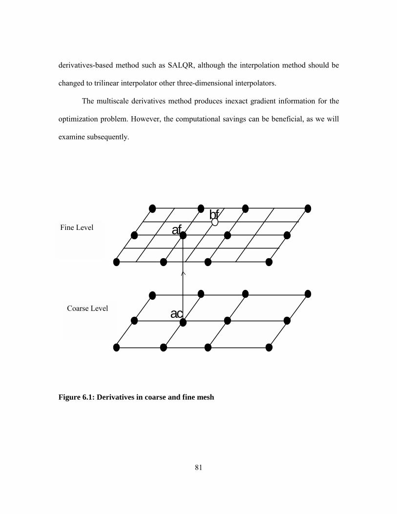
81
derivatives-based method such as SALQR, although the interpolation method should be
changed to trilinear interpolator other three-dimensional interpolators.
The multiscale derivatives method produces inexact gradient information for the
optimization problem. However, the computational savings can be beneficial, as we will
examine subsequently.
Fine Level
Coarse Level
ac
af bf
Figure 6.1: Derivatives in coarse and fine mesh
Fine Level
Coarse Level
82
6.3 Theoretical Estimation of the Computational Savings
The computing savings can be estimated by looking at how many derivatives
values were not calculated through the one-sided divided difference method on the finest
mesh. The current method uses a uniform two-dimensional mesh refinement for
simplicity. In this case, the ratio of the number of nodes in the coarse mesh to that in the
fine mesh can be calculated as follows
41
)*2(*)*2(*
)1*2(*)1*2(*
** =≈
−−=
cnycnxcnycnx
cnycnxcnycnx
fnyfnxcnycnx (6.1)
where cnx and cny are the number of nodes in the x and y directions at the coarse mesh,
respectively, and fnx and fny are the number of nodes in the x and y directions at the fine
mesh, respectively. Hence, the computational saving is theoretically about 25%, not
including the computational cost of interpolation and the coarse grid derivatives
calculation, which are usually small compared to the one-sided divided difference
calculation on the fine mesh.
6.4 Results of Numerical Experiments for the Multiscale
Derivatives Method
To demonstrate the advantages of using V-cycle multiscale numerical derivatives,
a bilevel run was performed at Level 3 and Level 2 using the V-cycle multiscale
derivatives method, based on the test case used in Chapter 5. During our numerical
experiment, we found that the V-cycle multiscale derivatives produce good convergence
behavior during the initial iterations but cannot converge if such derivatives are used
83
during late iterations when the model required accurate predications of small
perturbations near the optimal solution. This result is understandable because V-cycle
multiscale derivatives are not the exact representations of the system response at the fine
mesh level. To take advantage of the computational savings provided by the V-cycle
multiscale derivatives and still obtain convergence, a simple switch mechanism was
implemented to switch from V-cycle multiscale derivatives to normal fine-mesh
numerical derivatives once the percentage change in the objective function value between
two consecutive iterations becomes small, indicating that the current solution is likely
within the neighborhood of the optimal solution and more accurate derivatives are
required. The percentage change Ps is defined as follows
Ps = %100)( 1 ×
−+
i
ii
objobjobj
(6.2)
where obji+1 and obji are the objective function values at iteration i+1 and i, respectively.
In this problem, Ps = 0.6% is chosen, which means that when the percentage change is
less than or equal to 0.6%, the next iteration will switch to using normal one-sided
forward divided difference numerical derivatives on the fine mesh. The result of this
procedure is shown in Figure 6.2, along with the normal numerical derivative results at
Level 3 for comparison.
As can be seen from Figure 6.2, the CPU time per iteration using normal
numerical derivatives at Level 3 is about 2.3 hours, while the V-cycle multiscale
derivatives is about 1.8 hours, which is about a 22% reduction. This is close to the
theoretical prediction of 25%. The total computing time for using V-cycle multiscale
84
derivatives with the switching mechanism is about 27 hours and the total computing time
for using numerical derivatives alone is about 37.8 hours, which is about a 29% reduction
in computing time. The higher overall reduction results from the V-cycle multiscale
derivatives method with switching mechanism requiring a fewer total number of
iterations (14 iterations vs. 16 iterations for numerical derivatives alone). It is believed
that the reduction in the number of iterations results from the model following a slightly
different search path with the multiscale derivatives; hence, this reduction may not
necessarily occur in other applications of this method. Note that the combined reduction
of using multiscale derivatives with switching mechanism over the previous analytical
derivatives method (117 hours, see Chapter 5) is about 77%, a significant improvement in
computational performance.
6.5 Summary
A framework for multiscale derivative implementation in an SALQR model has
been presented. Using the numerical derivatives implementation presented in Chapter 5,
the V-cycle multiscale derivative method approximated the derivatives at the fine level
by interpolating the derivatives from the coarser level, which provides a theoretical
reduction of 25% and an actual reduction of 22% per iteration in our case study. The total
computing time for using V-cycle multiscale derivatives for the case study with more
than 1,600 state variables represented approximately a 29% reduction in computing time
compared to the numerical derivatives method alone, or a 77% reduction compared to the
previous analytical derivatives method. These methods clearly provide a substantial

85
reduction in computing time relative to previous methods even for a relatively small test
case. When these methods are combined with the one-way spatial multiscale method (Liu
et al. 2001, also see Chapter 4), even greater savings should be possible. A
comprehensive study of all of the multiscale methods developed in this work will be
presented in the next chapter.
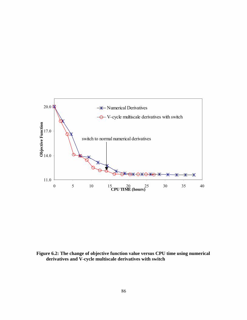
86
11.0
14.0
17.0
20.0
0 5 10 15 20 25 30 35 40CPU TIME (hours)
Obj
ectiv
e Fu
nctio
n
Numerical Derivatives
V-cycle multiscale derivatives with switch
switch to normal numerical derivatives
Figure 6.2: The change of objective function value versus CPU time using numerical
derivatives and V-cycle multiscale derivatives with switch
87
Chapter 7
Full Multiscale Approach for SALQR Model
As previous chapters have shown, individual methods, including one-way spatial
multiscale method (Chapter 4), efficient numerical derivatives method (Chapter 5), and
multiscale derivatives method (Chapter 6), can significantly reduce the computational
time associated with solving bioremediation optimal control model. To further reduce the
computing time, a full multiscale approach is developed in this Chapter, which combines
the methods developed in the previous chapters. Several strategies are also investigated to
improve the computational performance of the approach further. Case studies show the
computational savings with different configurations of different components of the full
multiscale approach.
7.1 Description of the Methodology
The full multiscale computational approach is a combination of the one-way
spatial multiscale method, efficient numerical derivatives method, and multiscale V-cycle
derivatives method. As can be seen from Figure 7.1, this method starts from the coarsest
mesh (Level 1) and solves the model to convergence. Then the converged results are
interpolated to the finer mesh (Level 2) and the model runs using the converged results
88
from Level 1 as the starting point. At Level 2, when the derivatives are needed in the
backward sweep, the V-cycle multiscale derivatives method developed in Chapter 6 is
used. The model switches back to the coarser level (Level 1), obtains the coarse grid
derivatives, and then interpolates back to the current level using a standard bilinear
interpolator. The efficient one-sided divided difference method presented in Chapter 5
(also see Liu and Minsker, 2001, in press) is used to calculate the numerical derivatives
so that those derivatives that cannot be interpolated can be calculated separately on Level
2. Once the model converges at Level 2, the solution is interpolated to the finer mesh and
a similar procedure is performed at Level 3. This process continues until the model
reaches the finest level (in Figure 7.1, the finest level is Level 3) and converges.
A more general description of the methodology is given as follows.
(1) For a given problem, set up a hierarchy of meshes where the mesh sizes h1>
h2>.>hL-1 > hL, L being the finest level with the desired level of accuracy
and 1 being the coarsest level.
(2) Starting from the coarsest level (Level 1), solve the model (both forward and
backward sweep) to convergence.
(3) For Level = 2 to L
a. Interpolate the results from Level1 to Level using a bilinear
interpolator.
b. Start with this value to perform a two-level cycle of the V-cycle
multiscale derivatives calculation.
i. Calculate derivatives at Level-1.
89
ii. Interpolate derivatives to Level using standard bilinear
interpolation.
iii. Calculate remaining derivatives at Level.
c. Continue until convergence at Level.
(4) Stop after convergence at the finest level.
Notice that in Figure 7.1, the single-line arrow stands for the interpolation of the
solution between coarse level and fine level as discussed in Chapter 4, and the double-
line arrow stands for the switch and interpolation of the derivatives between coarse level
and fine level as discussed in Chapter 6. Since the operation targets are different in these
two cases, different representations are used in Figure 7.1.
The finest level is determined by the spatial accuracy requirement of the
simulation model. As a rule of thumb, the finite element method requires a Peclet number
less than 2 for modeling accuracy in space. Since the full multiscale approach focuses on
computational time reduction in space, it is not necessary to require the Peclet number to
be less than 2 at all levels except the finest level.
7.2 Strategies for Performance Enhancement
Several possible strategies have been investigated to enhance the performance of
the full multiscale approach presented in Section 7.1. These strategies are discussed
below.
90
7.2.1 Local Effect of the Derivatives
When examining the spatial structure of the first derivatives of the transition
equation with respect to the state variables, we found two distinct regions: a peak region
and a smooth region. Figure 7.2 shows an example of the spatial structure of the first
derivative of oxygen concentration at the beginning of management period 2 with respect
to the biomass concentration at the beginning of management period 1(tb
to
cc
,
1,
∂∂ + in Appendix
C, where t =1). We call this the local-effect of the derivatives, which means that a
small perturbation of the value of one state variable can only have significant effect in the
next time step in its surrounding area but will have little effect in remote areas.
To solve the derivatives at the fine level only at the peak area, the boundary
conditions must be obtained from the coarser grid derivatives calculation. This was done
by performing a coarse grid perturbed simulation run and then using the interpolated state
variables at the finer grid as the boundary conditions for the peak areas simulation. One-
sided forward difference was then used to calculate the derivatives at the peak area.
Exploiting this type of local structure has been quite successful for solution of
PDEs (Brandt 2001) and it initially appeared quite promising for derivative calculations
as well. However, this local-effect strategy was not sufficiently accurate for calculating
derivatives. The errors come from two factors: the approximated boundary conditions
derived from the coarse grid simulation and the error propagation due to the transition in
time during one management period. The derivatives can be off by several orders of
magnitude even though satisfactory state values can be obtained.
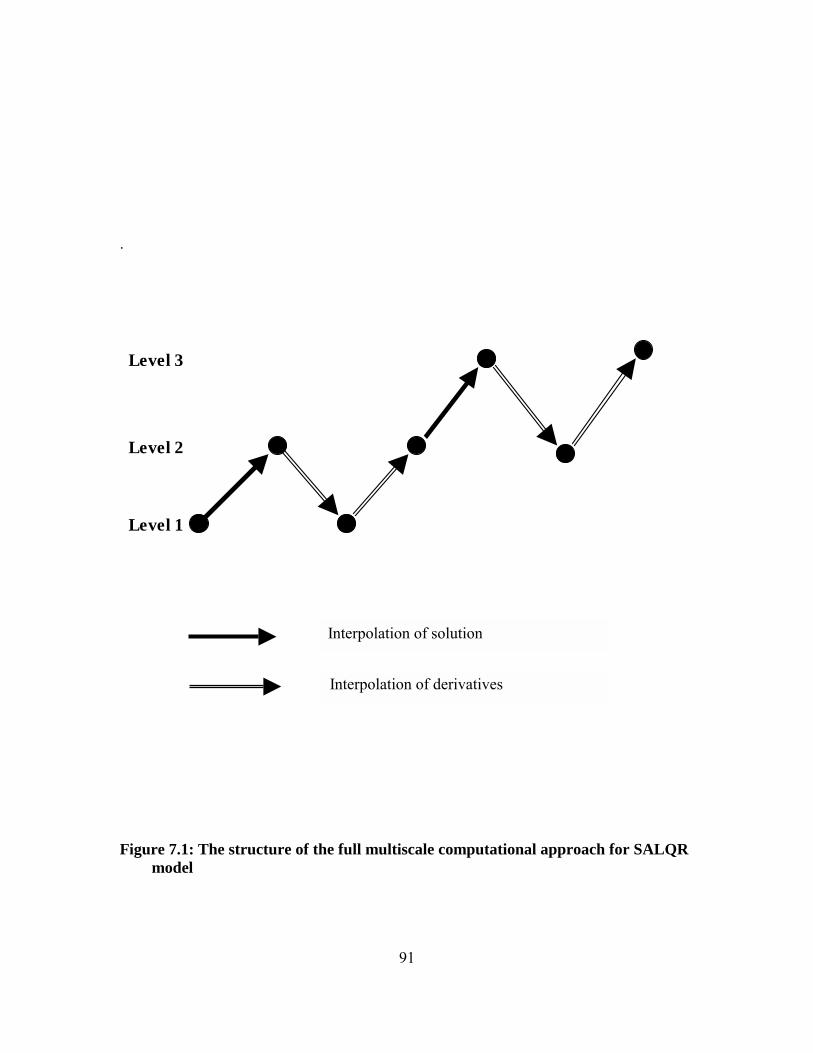
91
.
Level 1
Level 2
Level 3
Figure 7.1: The structure of the full multiscale computational approach for SALQR
model
Interpolation of solution
Interpolation of derivatives
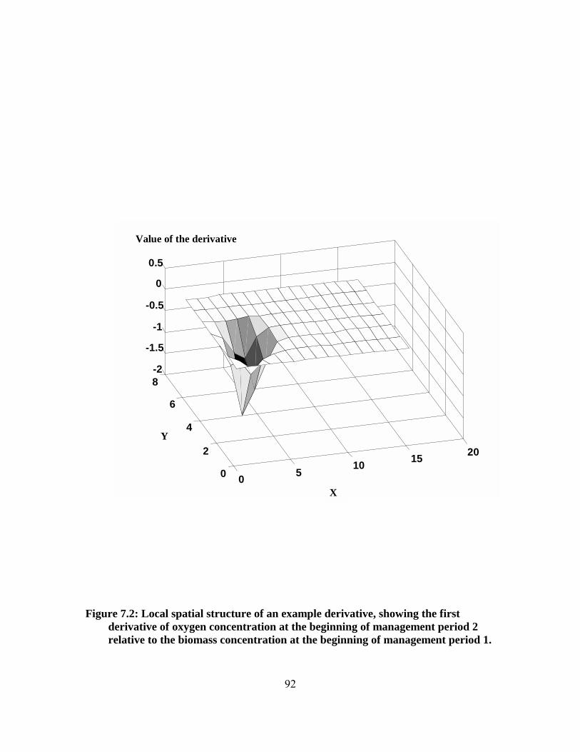
92
0 5 10 15 20
0
2
4
6
8-2
-1.5
-1
-0.5
0
0.5
X
Y
Value of the derivative
Figure 7.2: Local spatial structure of an example derivative, showing the first
derivative of oxygen concentration at the beginning of management period 2 relative to the biomass concentration at the beginning of management period 1.
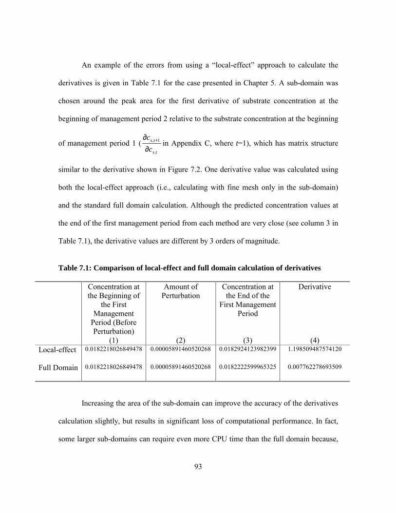
93
An example of the errors from using a local-effect approach to calculate the
derivatives is given in Table 7.1 for the case presented in Chapter 5. A sub-domain was
chosen around the peak area for the first derivative of substrate concentration at the
beginning of management period 2 relative to the substrate concentration at the beginning
of management period 1 (ts
ts
cc
,
1,
∂∂ + in Appendix C, where t=1), which has matrix structure
similar to the derivative shown in Figure 7.2. One derivative value was calculated using
both the local-effect approach (i.e., calculating with fine mesh only in the sub-domain)
and the standard full domain calculation. Although the predicted concentration values at
the end of the first management period from each method are very close (see column 3 in
Table 7.1), the derivative values are different by 3 orders of magnitude.
Table 7.1: Comparison of local-effect and full domain calculation of derivatives
Concentration at the Beginning of
the First Management
Period (Before Perturbation)
(1)
Amount of Perturbation
(2)
Concentration at the End of the
First Management Period
(3)
Derivative
(4) Local-effect 0.0182218026849478 0.00005891460520268 0.0182924123982399 1.198509487574120
Full Domain 0.0182218026849478 0.00005891460520268 0.0182222599965325 0.007762278693509
Increasing the area of the sub-domain can improve the accuracy of the derivatives
calculation slightly, but results in significant loss of computational performance. In fact,
some larger sub-domains can require even more CPU time than the full domain because,
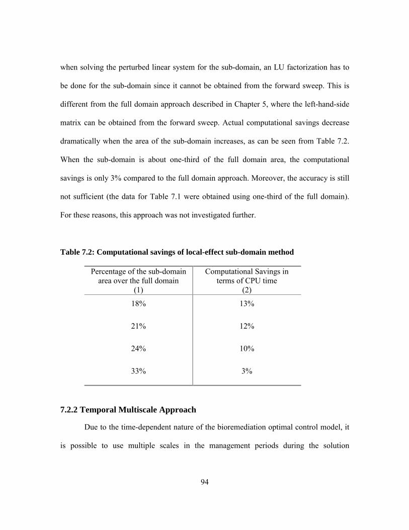
94
when solving the perturbed linear system for the sub-domain, an LU factorization has to
be done for the sub-domain since it cannot be obtained from the forward sweep. This is
different from the full domain approach described in Chapter 5, where the left-hand-side
matrix can be obtained from the forward sweep. Actual computational savings decrease
dramatically when the area of the sub-domain increases, as can be seen from Table 7.2.
When the sub-domain is about one-third of the full domain area, the computational
savings is only 3% compared to the full domain approach. Moreover, the accuracy is still
not sufficient (the data for Table 7.1 were obtained using one-third of the full domain).
For these reasons, this approach was not investigated further.
Table 7.2: Computational savings of local-effect sub-domain method
Percentage of the sub-domain area over the full domain
(1)
Computational Savings in terms of CPU time
(2)
18% 13%
21% 12%
24% 10%
33% 3%
7.2.2 Temporal Multiscale Approach
Due to the time-dependent nature of the bioremediation optimal control model, it
is possible to use multiple scales in the management periods during the solution
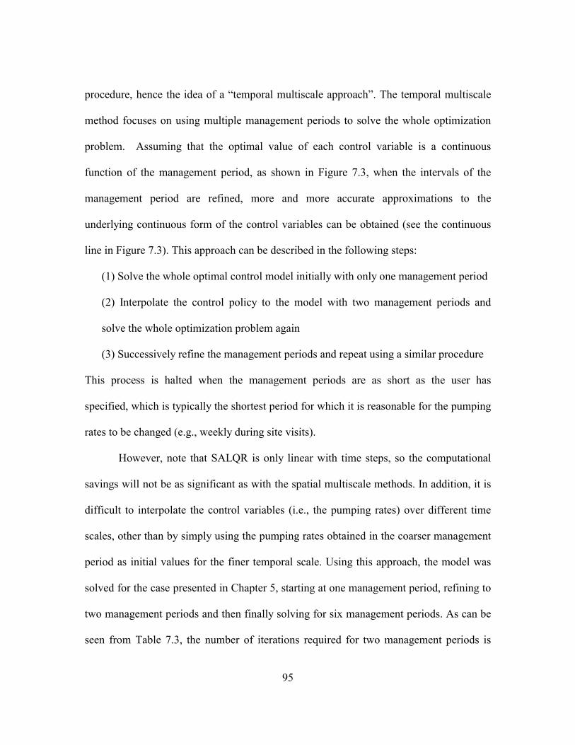
95
procedure, hence the idea of a temporal multiscale approach. The temporal multiscale
method focuses on using multiple management periods to solve the whole optimization
problem. Assuming that the optimal value of each control variable is a continuous
function of the management period, as shown in Figure 7.3, when the intervals of the
management period are refined, more and more accurate approximations to the
underlying continuous form of the control variables can be obtained (see the continuous
line in Figure 7.3). This approach can be described in the following steps:
(1) Solve the whole optimal control model initially with only one management period
(2) Interpolate the control policy to the model with two management periods and
solve the whole optimization problem again
(3) Successively refine the management periods and repeat using a similar procedure
This process is halted when the management periods are as short as the user has
specified, which is typically the shortest period for which it is reasonable for the pumping
rates to be changed (e.g., weekly during site visits).
However, note that SALQR is only linear with time steps, so the computational
savings will not be as significant as with the spatial multiscale methods. In addition, it is
difficult to interpolate the control variables (i.e., the pumping rates) over different time
scales, other than by simply using the pumping rates obtained in the coarser management
period as initial values for the finer temporal scale. Using this approach, the model was
solved for the case presented in Chapter 5, starting at one management period, refining to
two management periods and then finally solving for six management periods. As can be
seen from Table 7.3, the number of iterations required for two management periods is
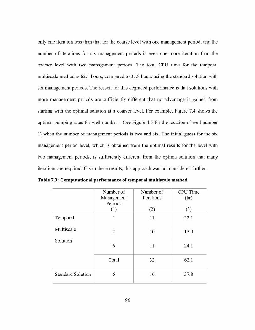
96
only one iteration less than that for the coarse level with one management period, and the
number of iterations for six management periods is even one more iteration than the
coarser level with two management periods. The total CPU time for the temporal
multiscale method is 62.1 hours, compared to 37.8 hours using the standard solution with
six management periods. The reason for this degraded performance is that solutions with
more management periods are sufficiently different that no advantage is gained from
starting with the optimal solution at a coarser level. For example, Figure 7.4 shows the
optimal pumping rates for well number 1 (see Figure 4.5 for the location of well number
1) when the number of management periods is two and six. The initial guess for the six
management period level, which is obtained from the optimal results for the level with
two management periods, is sufficiently different from the optima solution that many
iterations are required. Given these results, this approach was not considered further.
Table 7.3: Computational performance of temporal multiscale method
Number of Management
Periods (1)
Number of Iterations
(2)
CPU Time (hr)
(3)
1 11 22.1
2 10 15.9
Temporal
Multiscale
Solution 6 11 24.1
Total 32 62.1
Standard Solution 6 16 37.8
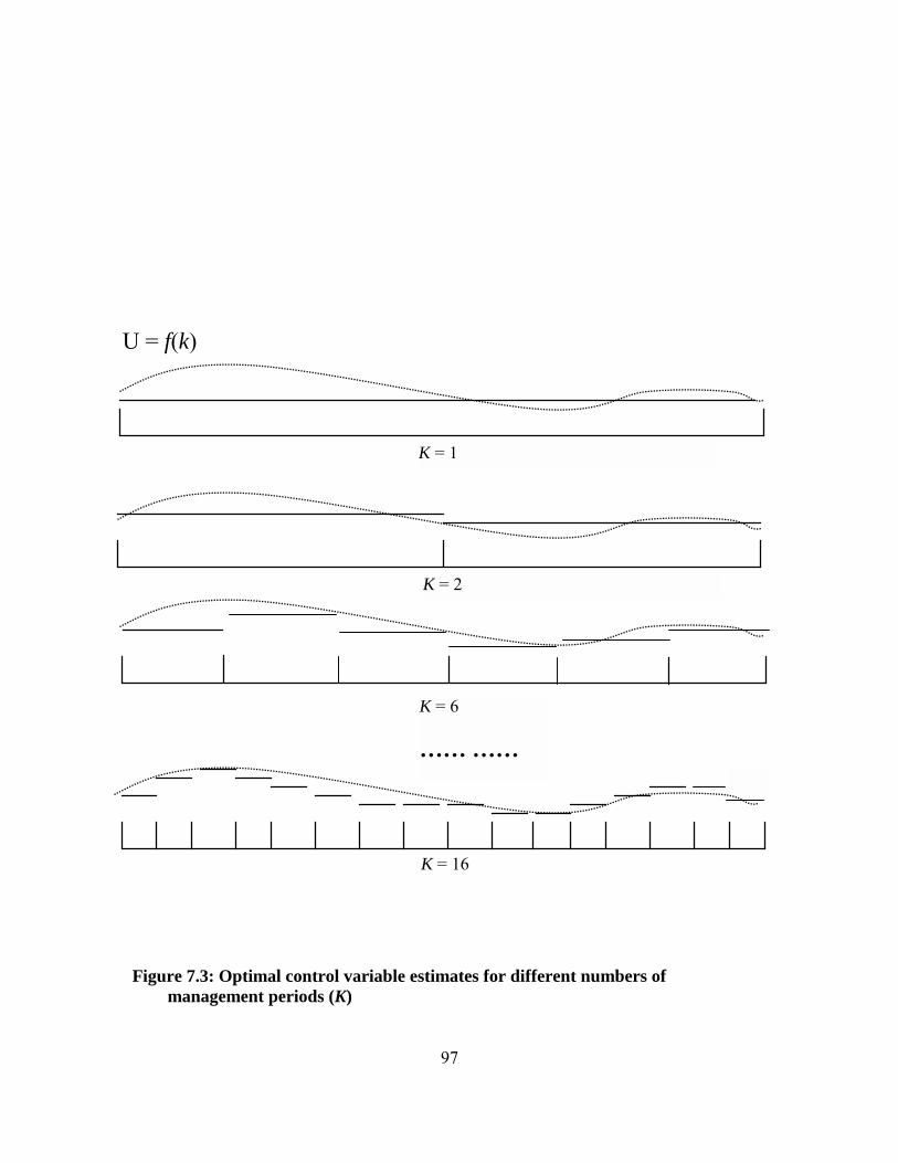
97
Figure 7.3: Optimal control variable estimates for different numbers of
management periods (K)
U = f(k)
K = 16
K = 1
K = 2
K = 6 …… ……
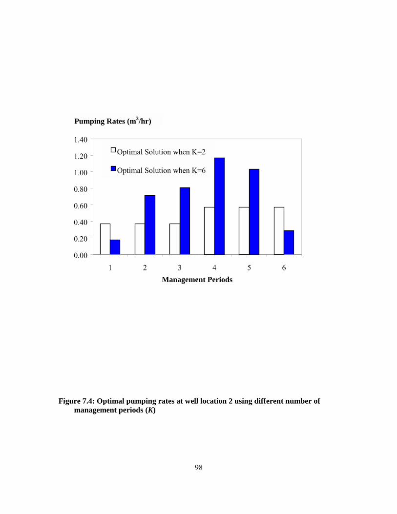
98
0.00
0.20
0.40
0.60
0.80
1.00
1.20
1.40
1 2 3 4 5 6Management Periods
Optimal Solution when K=2
Optimal Solution when K=6
Figure 7.4: Optimal pumping rates at well location 2 using different number of
management periods (K)
Pumping Rates (m3/hr)
99
7.2.3 Configuration of the Full Multiscale Method
As described in the first section of this chapter, the full multiscale method consists
of the following individual components: one-way spatial multiscale method, efficient
numerical derivatives, and V-cycle multiscale derivatives method. In order to obtain the
best possible computational performance of the full multiscale method, different
configurations of the individual components have been investigated.
Figure 7.5 shows the five configurations, or schema, that were tested. Schemas 1
to 3 use both the V-cycle derivatives calculation and the one-way spatial multiscale
method. For comparison, only the one-way spatial multiscale method is used in schema 4
and 5 with different starting levels. All five schemas use the numerical derivatives
approach because, as shown in Chapter 5, it is substantially more efficient than the
analytical derivatives approach. Moreover, the V-cycle multiscale derivatives method can
only be used with the numerical derivatives approach because it is dependent on
decoupling of the derivatives calculation.
Note that V-cycle multiscale derivatives can switch back and forth between more
than two levels, for example by calculating derivatives at Level 3 starting at Level 1.
However, since most of the computing time is still spent on the fine level (Level 3) and
coarser levels (Level 1) are not likely to improve accuracy, only a bilevel V-cycle
derivatives method is used in the configurations. A final note is that at the finest level,
which is usually determined by the accuracy requirement of the simulation model, it is
not advantageous to use the V-cycle derivatives method. At this stage, the SALQR
algorithm is fine-tuning pumping rates and the V-cycle approximation slows down
100
convergence. Variations of Schemas 1 through 3 were run with the V-cycle derivatives
approximation added at Level 4, but these runs did not converge within five iterations
(the maximum convergence required for schemas 1 through 3) and were halted. For this
reason, these schemas are not shown in Figure 7.4.
7.3 Results and Discussion for Full Multiscale Approach
To test the approaches developed in this chapter,, the case study presented in
Chapter 4 was used (see Table 4.2 for site characteristics and model parameters and
Figure 4.5 for the schematic view of the test site). The four-level mesh hierarchy
developed in Chapter 5 was implemented to test the schemas shown in Figure 7.5.
The first test of the full multiscale approach is to compare its performance to the
other methods, including solving the model at a single level with analytical derivatives
from Minsker and Shoemaker (1998a). Given the substantial computational effort
required for the analytical derivatives methods, this comparison was only performed at
Level 3 (see Table 5.1 for the level information). This comparison, given in Figure 7.6,
shows the advantage of using the full multiscale approach over other methods. In Figure
7.6, when using only a single grid (i.e., running the whole optimal control model at Level
3), the efficient numerical derivatives method outperforms the analytical derivatives with
a 68% reduction in computing time using a single grid (38 vs. 117 hours). The one-way
spatial multiscale method can be applied with either the numerical derivatives method or
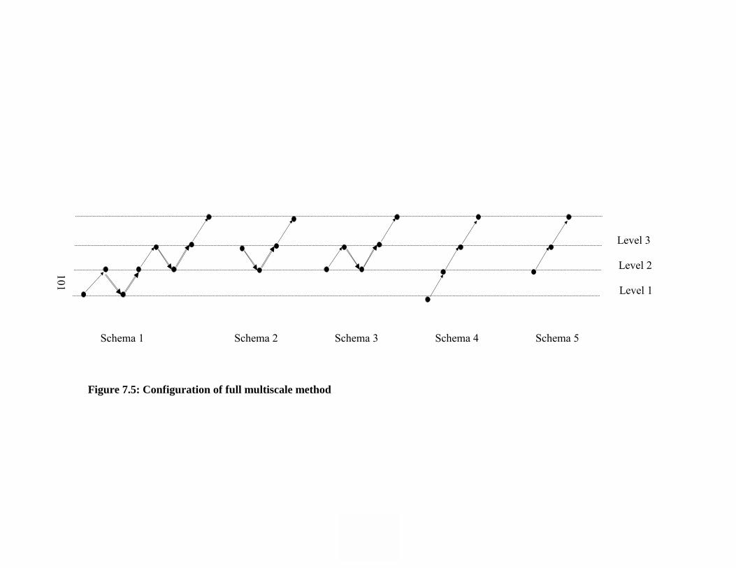
101
Schema 1 Schema 2 Schema 3 Schema 4 Schema 5
Figure 7.5: Configuration of full multiscale method
101
Level 3
Level 2
Level 1
102
the analytical derivatives method. Combining the one-way spatial multiscale method with
the efficient numerical derivatives method results in a 70% reduction in computing time
over the analytical derivatives single-grid approach and a 36% reduction over the one-
way spatial multiscale method with analytical derivatives. However, the one-way spatial
multiscale method provides only an additional 8% reduction over the single-grid case
when numerical derivatives are used.
Since analytical derivatives cannot be used in the V-cycle and full multiscale
derivatives method, only the efficient numerical derivatives method is used with those
methods. The V-cycle derivatives method and the full multiscale approach took about
29% and 32% less time to converge than the single-grid numerical derivatives approach,
respectively. The full multiscale method achieves a 78% computational savings over the
previous single-grid approach with analytical derivatives method. Note that much greater
savings would be achieved at Level 4 because the computational savings increase for
finer grids.
To find the best configuration of the full multiscale approach, several runs were
conducted using the schemas in Figure 7.5. The estimated running time for a Level 4 case
(which has about 6,500 state variables) using the previous analytical derivatives single-
grid model would be between 10 to 12 months, which is not practical to run the actual
model. As shown in Figure 7.7, the best performance is achieved by Schema 2, which
follows a checkmark stencil (see Figure 7.5) and found the optimal solution within 8.8
days. In fact, for Schema 2, the optimal control model was able to converge with only 3
additional iterations at the finest level (Level 4). The full multiscale approach starting
103
from Level 1 (i.e., Schema 1) is the second fastest with a total CPU time of 10.8 days.
These results are estimated to be more than 30 times faster than the previous optimal
control model using a single grid and analytical derivatives. Schema 3 finished with a
total CPU time of 11.9 days, which is slightly higher than Schema 2. Both Schemas 2 and
3 were able to converge with only 4 additional iterations at the finest level. It is possible
that Schema 2 follows a slightly different search path and thus converges faster.
Schemas 1, 2 and 3 are all significantly faster than Schemas 4 and 5, indicating
the advantages of incorporating the V-cycle derivatives approach in the full multiscale
method. Both Schemas 4 and 5 use only the one-way spatial multiscale method with
efficient numerical derivatives and converge with only 5 additional iterations at the finest
level. Since both schema 4 and 5 do not use the V-cycle derivatives calculation, they
exhibit a loss of performance.
These results show that inexact derivatives at the early stage of the optimization
(as in the V-cycle derivatives method) can play a significant role in reducing computing
time, especially for large-scale cases. In addition, all of the schemas show the importance
of considering the interaction of PDE discretization and the optimization procedure. Due
to the nature of PDE-constrained optimization problems, where solving PDEs is only the
subproblem of the optimization problem, refining optimization solutions must be carried
out simultaneously with the mesh refinement for the PDE. As can be seen from Figure
7.7, multiple spatial scales and mesh refinement can provide significant computational
savings while still maintaining satisfactory convergence of the optimization algorithm in
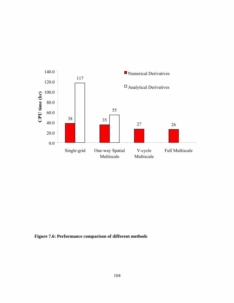
104
38 3527 26
117
55
0.0
20.0
40.0
60.0
80.0
100.0
120.0
140.0
Single-grid One-way SpatialMultiscale
V-cycleMultiscale
Full Multiscale
Numerical Derivatives
Analytical Derivatives
Figure 7.6: Performance comparison of different methods
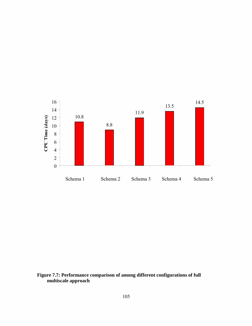
105
10.88.8
11.913.5
14.5
02468
10121416
Figure 7.7: Performance comparison of among different configurations of full
multiscale approach
Schema 1 Schema 2 Schema 3 Schema 4 Schema 5
106
the early stages of the search. However, once the model reaches the finest level, it is near
the optimal solution and accurate derivatives are necessary. This is a general principle for
solving any PDE-constrained optimization problem regardless of the optimization
algorithm used.
Finally, the results indicate that three spatial levels are usually sufficient to
provide good results and computational savings. For example, Schemas 1 and 3 only
differ in the starting level and the total number of levels, but the difference in terms of
computing time is only about 10%. Similarly, Schemas 4 provides only 7%
computational savings over schema 5, which has one less level. Moreover, with four
levels it is more difficult to ensure that pumping well locations remain in the coarsest
mesh. While methods exist to interpolate wells between mesh points (e.g., Huang and
Mayer 1997), it is not clear that the computational savings would be worth the added
complexity.
7.4 Summary
We presented a full multiscale method for an optimal control model of
groundwater in-situ bioremediation in this chapter. This method integrates the one-way
spatial multiscale method, the efficient numerical derivatives method, and the V-cycle
multiscale numerical derivatives method developed in previous chapters. Application of
the method starts from the coarsest mesh and solves for the optimal solution at that level,
then uses the optimal solution obtained as the initial guess for the finer mesh. While at
the finer mesh, the method switches back to the coarser mesh to solve for the derivatives
107
and uses those derivatives to interpolate back to the finer mesh. This procedure continues
until convergence is achieved at the finest level.
Application of the full multiscale method to a case with about 6,500 state
variables shows substantial performance gains over previous approaches. The CPU time
for the full multiscale approach ranges between 8.8 days and 11.9 days, depending on the
configuration of the approach. These are significant computational savings compared to
the previous single-grid model using analytical derivatives, which is estimated to require
nearly one year to converge. Combinations of the one-way spatial multiscale method,
efficient numerical derivatives and V-cycle multiscale derivatives method always
outperform methods with only one individual component.
The interaction of PDE discretization and optimization is discovered in this study.
Since solving PDEs is only a subproblem with PDE-constrained optimization, it is critical
that refining optimization solutions be performed simultaneously with the mesh
refinement for the PDE. At the early stage of the optimization, a coarse mesh for the PDE
can be used to facilitate broad search of the decision space. Once the search is close to the
optimal, a finer mesh is needed for the PDEs to provide more accurate information on
state variables and expedite fine-tuning of the optimal solution. This is a general principle
for solving any PDE-constrained optimization problem regardless of the optimization
algorithm used. For the derivative-based optimization algorithms, such as the SALQR
method used in this research, V-cycle derivatives calculation is very beneficial for the
early stage of the optimization and should be used in conjunction with the one-way
spatial multiscale method. We found that using the V-cycle multiscale derivatives method
108
at the finest level is not beneficial. Once the model reaches the finest level, it is already
near the optimal solution, and inexact derivatives are not beneficial for fine tuning the
optimal solution.
The number of levels used in the full multiscale approach can be traded off with
the additional complexities of interpolating pumping rates at the coarsest level when well
locations are between mesh nodes. As a rule of thumb, a three-level mesh hierarchy
appears to be sufficient for obtaining the greatest performance gains. In the case study
shown, there is no significant difference between the four-level and three-level full
multiscale method, as indicated by Schemas 1 and 3, as well as Schemas 4 and 5 because
most of the computing time is still spent on the finest level.
109
Chapter 8
Concluding Remarks 8.1 Conclusions
Applying formal optimization algorithms such as the SALQR method to assist in
optimal design of large-scale in-situ bioremediation of groundwater is expected to be
highly rewarding because substantial cost savings could be achieved if optimal designs
can be used. However, solving an optimal control model for in-situ bioremediation design
poses a computational challenge even for the most advanced supercomputing power
available today. The results and insights obtained in this research can substantially reduce
the computational burden associated with solving the SALQR optimal control model for
in-situ bioremediation. Furthermore, the multiscale methods developed in this research
are also expected to be applicable for other large-scale PDE-constrained optimization
problems, which are commonly encountered in various engineering and science
disciplines.
The SALQR optimal control model of in-situ bioremediation of groundwater uses
a management period formulation, where the pumping rates change only every
management period instead of every simulation period. Due to the dynamics and
nonlinearity of bioremediation systems, the simulation model usually requires small
110
simulation time steps. Thus, it is necessary to use a management period formulation to
avoid changing pumping rates too frequently and unrealistically. However, this causes a
significant computational burden in calculating the first derivatives of the transition
equation with respect to the state and control variables, which are needed for the SALQR
method. Our analysis found that the two-step analytical derivatives method is the
computational bottleneck of the SALQR optimal control model of in-situ bioremediation
with a management period formulation, requiring over 90% of the total computing time.
The first step requires a matrix inversion and the second step requires dense matrix
multiplication, both of which are on the order of N3, where N is the number of state
variables. Since bioremediation models usually need a fine numerical mesh, which means
large numbers of state variables, the cubic growth rate of the computing time with respect
to the number of state variables prohibits the application of this model to large-scale
design. To improve the computational performance of the model and overcome the
scale issue, new approaches to reduce both the total number of iterations and the CPU
time per iteration must be developed. The multiscale methods developed in this work
meet such objectives.
Since the bioremediation optimal control model is governed by a set of nonlinear
PDEs, which describe the system response under given pumping rates, an accurate
solution of the simulation model is necessary. However, the discretization of PDEs
introduces a large number of unknown state variables if only a single fine-grid model is
used. Because solving PDEs is only a subproblem of optimization in our study, we must
search for the optimal pumping rates and obtain accurate simulation results
111
simultaneously. The full multiscale method developed in this work achieves this goal by
using approximate solutions early in the run when a broad search of the decision space is
being performed. As the solution becomes more refined later in the run, more accurate
estimates are needed to finetune the solution and finer spatial discretizations are used.
The full multiscale approach integrates a one-way spatial multiscale method, an
efficient numerical derivatives method, and a V-cycle multiscale derivatives method. The
one-way spatial multiscale method proceeds one-way from the coarsest the finest mesh,
with the solution successively interpolated from coarse to fine level. This method is
applicable to any PDE-constrained optimization problems, as long as the governing PDEs
can be discretized into different spatial levels. For derivative-based optimization
algorithms, the one-way spatial multiscale method is independent of the approach used to
calculate derivatives (i.e., analytical or numerical derivatives). Application of the method
to a case study showed over 50% reduction of computing time relative to the previous
single-grid model.
The efficient numerical derivatives method exploits the procedure for calculating
the first derivatives of the transition equations with respect to the state variables and
reduces computational effort by an order of magnitude compared to the previous
analytical derivative method. The numerical derivatives method also decouples the
calculation of the derivatives at different nodes in the spatial discretization mesh so that
V-cycle multiscale derivatives method can be applied.
The V-cycle multiscale derivatives method approximates the fine-grid derivatives
by first switching back to the coarser level to obtain the coarser-grid derivatives and then
112
interpolating back to the fine level. These inexact derivatives values are beneficial only
for the early stage of the optimization when large changes in the pumping rates are made
and approximate response estimates are sufficient. About 25% reduction of computing
time can be achieved by using the V-cycle multiscale derivatives method in theory and
about 29% reduction in our case study.
Integrating the power of the one-way spatial multiscale method, the efficient
numerical derivatives method and the V-cycle multiscale derivatives method enables
solution of a case with about 6,500 state variables within 8.8 to 11.9 days, compared to
one year needed by the original single-grid model with analytical derivatives.
Various modeling issues associated with using multiscale methods for optimal
bioremediation design were identified in this research. Since multiple spatial scales are
used in this model, there is no need to require the Peclet number to be within 2 for the
finite element mesh at all levels except the finest level. The dispersivity values can also
be changed to higher values at the coarser levels to overcome any numerical difficulties
since the Peclet number may be too high at the coarser levels. The penalty weight used at
different levels is also critical to the search for optimal pumping rates when the model
moves up to a higher level. Our study shows that good results can be obtained when the
penalty weight is decreased after interpolation to a finer mesh and when a terminal
penalty weight is used that gives a maximum violation of the substrate concentration
constraints of less than 1% of the standard. Finally, when designing the full multiscale
approach, the number of levels can be traded off with the ease of setting up the pre-
selected candidate pumping wells to avoid discontinuity. A three-level mesh hierarchy
113
was found to be sufficient for satisfactory performance in the case study examined in this
work.
8.2 Future Work
There are a number of possible future directions that could be pursed for
improving the multiscale methods developed in this work. Since the efficient numerical
derivatives method developed in this work decouples the calculation of derivatives at
different nodes, parallelization of the independent calculations of each derivative can be
implemented readily. This will further reduce the cost of computing time per iteration and
thus enable very large-scale design.
Another possible research direction is to use adaptive mesh refinement to
effectively control the problem size even for highly heterogeneous sites. This would
require much more sophisticated and advanced simulation models to be coupled with the
optimal control algorithm. The full multiscale approach developed in this work can still
be used in this context. However, the number of state variables will grow less
dramatically than with the uniform mesh refinement method used in this research.
Changing the governing PDE equations will likely change the way the derivatives are
calculated if the SALQR method is used as the optimization algorithm, so more research
would be needed on how to efficiently calculate the derivatives in such a context. The
one-way spatial multiscale method and V-cycle derivatives calculation can be adapted to
other 2-D or 3-D simulation models without major difficulties.
114
Since the current SALQR algorithm is relatively slow when it is near the optimal
solution, it is possible to explore some new ideas on how to consider the augmented
objective function as a level-dependent function and how to use multiscale methods to
expedite the search in the objective function space. Since the penalty function
incorporates the state variables into the objective function, the augmented objective
function can be considered as level dependent. Thus it might be possible to design a
multiscale method where the coarse grid problem is to find the descent gradient direction
for the fine grid optimization problem.
It is also possible to extend the application of the multiscale methods developed in
this work into other PDE-constrained optimization problems, such as groundwater
inverse problems. Combining multiscale methods with other optimization algorithms
(both derivative-based methods such as SQP and non-derivative-based methods such as
evolutionary algorithms) is also possible.
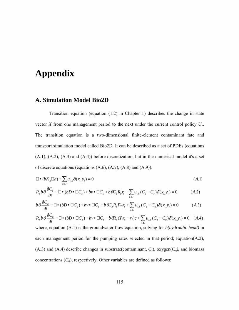
115
Appendix
A. Simulation Model Bio2D
Transition equation (equation (1.2) in Chapter 1) describes the change in state
vector X from one management period to the next under the current control policy Uk.
The transition equation is a two-dimensional finite-element contaminant fate and
transport simulation model called Bio2D. It can be described as a set of PDEs (equations
(A.1), (A.2), (A.3) and (A.4)) before discretization, but in the numerical model it's a set
of discrete equations (equations (A.6), (A.7), (A.8) and (A.9)).
)4.(0)()()()(
)3.(0)()()(
)2.(0)()()(
)1.(0)()(
,'
,
,'
,
,'
,
,,
AyxCCucrrYRbCbvCbDt
CbR
AyxCCurFRCbCbvCbDt
Cb
AyxCCurRCbCbvCbDt
CbR
AyxuhbK
iibUi
bkibscbbbb
b
iioUi
okisosbbooo
iisUi
skisbbsss
s
iiUi
kih
=−+−−∇•+∇••∇−∂
∂
=−++∇•+∇••∇−∂
∂
=−++∇•+∇••∇−∂
∂
=+∇•∇
∑
∑
∑
∑
∈
∈
∈
∈
δθθ
δθθ
δθθ
δ
where, equation (A.1) is the groundwater flow equation, solving for h(hydraulic head) in
each management period for the pumping rates selected in that period; Equation(A.2),
(A.3) and (A.4) describe changes in substrate(contaminant, Cs), oxygen(Co), and biomass
concentrations (Cb), respectively; Other variables are defined as follows:
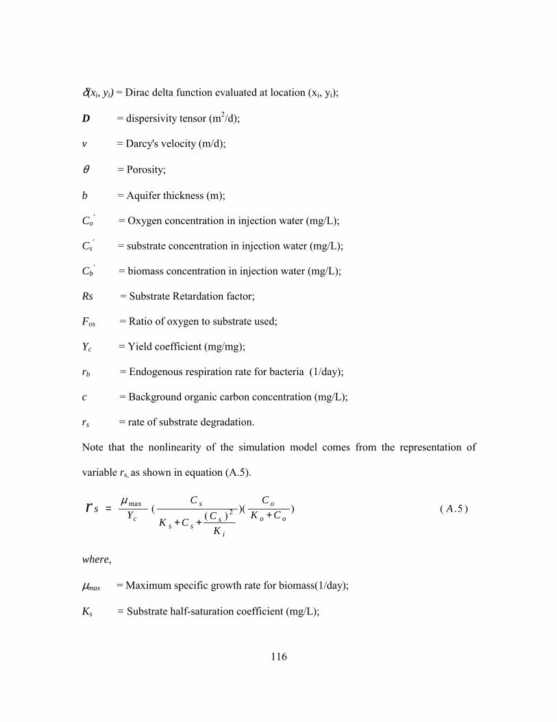
116
δ(xi, yi) = Dirac delta function evaluated at location (xi, yi);
D = dispersivity tensor (m2/d);
v = Darcy's velocity (m/d);
θ = Porosity;
b = Aquifer thickness (m);
Co' = Oxygen concentration in injection water (mg/L);
Cs' = substrate concentration in injection water (mg/L);
Cb' = biomass concentration in injection water (mg/L);
Rs = Substrate Retardation factor;
Fos = Ratio of oxygen to substrate used;
Yc = Yield coefficient (mg/mg);
rb = Endogenous respiration rate for bacteria (1/day);
c = Background organic carbon concentration (mg/L);
rs = rate of substrate degradation.
Note that the nonlinearity of the simulation model comes from the representation of
variable rs, as shown in equation (A.5).
)5.())()(
( 2max ACK
C
KCCK
CYs
oo
o
i
sss
s
cr +
++=
µ
where,
µmax = Maximum specific growth rate for biomass(1/day);
Ks = Substrate half-saturation coefficient (mg/L);
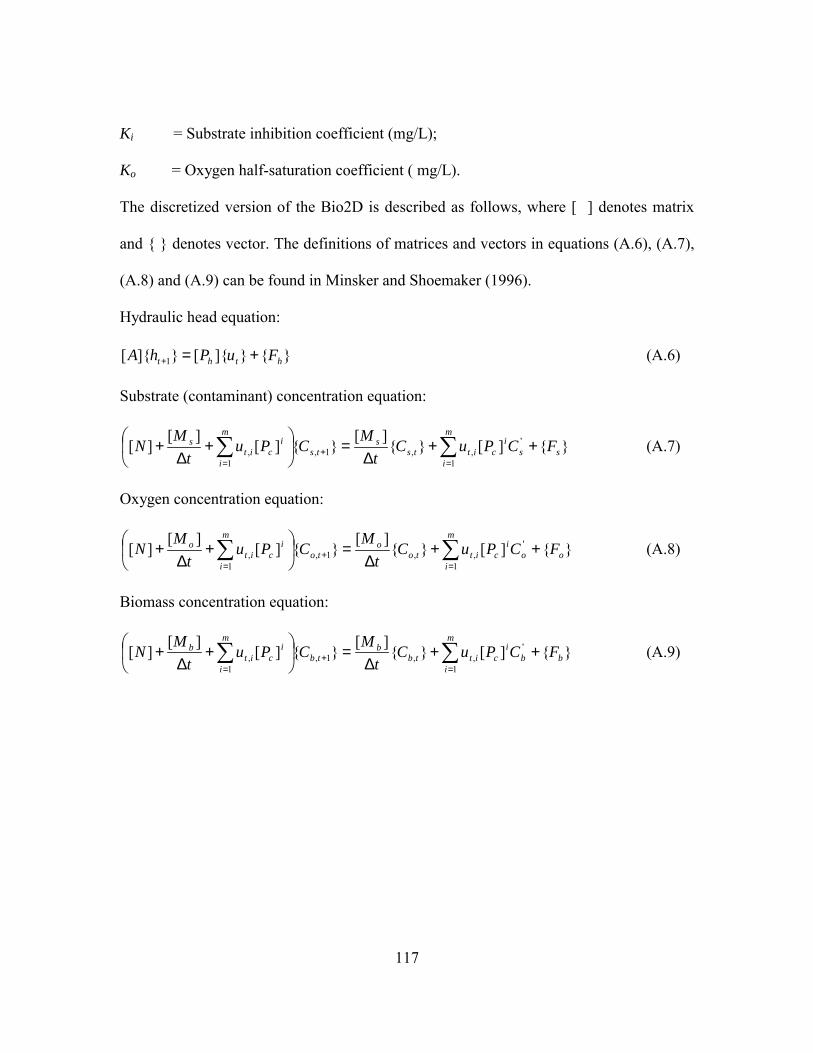
117
Ki = Substrate inhibition coefficient (mg/L);
Ko = Oxygen half-saturation coefficient ( mg/L).
The discretized version of the Bio2D is described as follows, where [ ] denotes matrix
and denotes vector. The definitions of matrices and vectors in equations (A.6), (A.7),
(A.8) and (A.9) can be found in Minsker and Shoemaker (1996).
Hydraulic head equation:
][][ 1 htht FuPhA +=+ (A.6)
Substrate (contaminant) concentration equation:
][][
][][
][ '
1,,1,
1, ss
m
i
icitts
sts
m
i
icit
s FCPuCt
MCPut
MN ++∆
=
+∆
+ ∑∑=
+=
(A.7)
Oxygen concentration equation:
][][
][][
][ '
1,,1,
1, oo
m
i
icitto
oto
m
i
icit
o FCPuCt
MCPut
MN ++∆
=
+∆
+ ∑∑=
+=
(A.8)
Biomass concentration equation:
][][
][][
][ '
1,,1,
1, bb
m
i
icittb
btb
m
i
icit
b FCPuCt
MCPut
MN ++∆
=
+∆
+ ∑∑=
+=
(A.9)
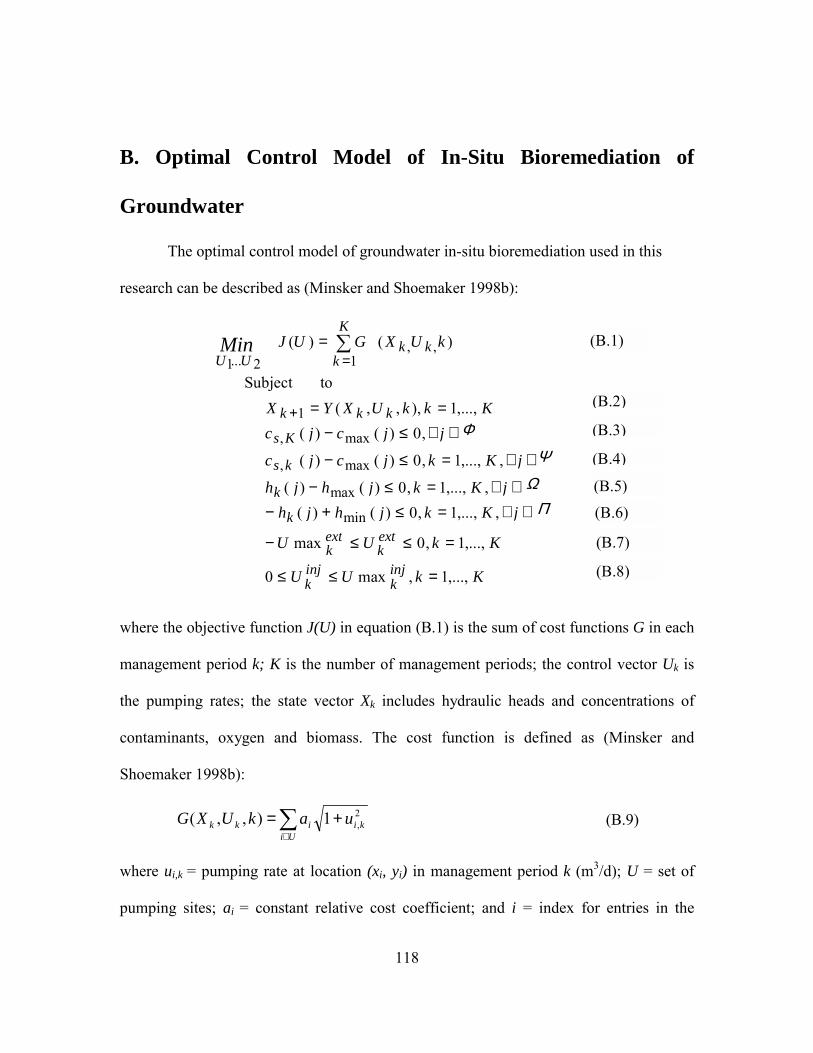
118
B. Optimal Control Model of In-Situ Bioremediation of
Groundwater
The optimal control model of groundwater in-situ bioremediation used in this
research can be described as (Minsker and Shoemaker 1998b):
K k U U
K k U U
j K k j h j h j K k j h j h
j K k j c j c
j j c j c K k k U X Y X
to Subject
k U X G U J
inj k
inj k
ext k
extk
k
k
k s
K s
kk k
k k K
k UU Min
,..., 1 , max 0
,..., 1 , 0 max
, ,..., 1 , 0 ) ( ) ( , ,..., 1 , 0 ) ( ) (
, ,..., 1 , 0 ) ( ) (
, 0 ) ( ) ( ,..., 1 ), , , (
) ( ) (
min max
max ,
max ,
1
,,12 ... 1
= ≤ ≤
= ≤ ≤ −
∈ ∀ = ≤ + − ∈ ∀ = ≤ −
∈ ∀ = ≤ − ∈ ∀ ≤ −
= =
=
+
= ∑
Π
Ω
Ψ
Φ
(B.1)
(B.2)
(B.3)
(B.4)
(B.5)
(B.6)
(B.7)
(B.8)
where the objective function J(U) in equation (B.1) is the sum of cost functions G in each
management period k; K is the number of management periods; the control vector Uk is
the pumping rates; the state vector Xk includes hydraulic heads and concentrations of
contaminants, oxygen and biomass. The cost function is defined as (Minsker and
Shoemaker 1998b):
2,1),,( ki
Uiikk uakUXG +=∑
∈ (B.9)
where ui,k = pumping rate at location (xi, yi) in management period k (m3/d); U = set of
pumping sites; ai = constant relative cost coefficient; and i = index for entries in the
119
control vector Uk. Note that in this cost function, Xk is only an implicit variable that
affects Uk through equations (B.3) and (B.4).
The transition equation (B.2) describes the change in state vector Xk from one
management period to the next under the current control policy Uk. The transition
equation Y(Xk, Uk, k) is a two-dimensional finite-element contaminant fate and transport
simulation model called Bio2D.
Equations (B.3)-(B.8) are constraints, where cmax(j) = water quality goal at node j
(mg/L); cs,k(j) = substrate concentration in period k at node j (mg/L); Φ = set of nodes
with monitoring wells where water-quality compliance must be attained by the end of the
cleanup; Ψ = set of nodes with monitoring wells at the downgradient end of the solution
domain where water quality compliance must be maintained in every management
period; hmax(j) = maximum hydraulic head allowed at node j in period k (m); Ω = set of
nodes with injection wells; hmin(j) = minimum hydraulic head allowed at node j in periods
k (m); Π = set of nodes with extraction wells; hk(j) is the hydraulic head in period k at
node j (m); extkU max = maximum allowed extraction pumping rate vector in period k
(m3/d); extkU = extraction rate vector in period k ((m3/d); inj
kU max = maximum allowed
injection pumping rate vector in period k (m3/d) and injkU = extraction rate vector in
period k (m3/d).
The constraints in equation (B.3) ensure that the water-quality standard will be
met at the specified monitoring wells by the end of the clean-up period. The constraints
listed in (B.4) prevent the contaminant plume from migrating by requiring contaminant
120
concentrations at the downgradient edge of the solution domain to remain below the
water-quality goal in every management period. The hydraulic head constraints in (B.5)
are needed to prevent the model from selecting injection rates that cause unrealistically
high hydraulic heads. Similarly, the constraints in (B.6) prevent excessively low
hydraulic heads due to high rates of extraction pumping. Constraints (B.7) and (B.8) set
lower and upper bounds on the pumping rates at extraction and injection wells,
respectively. Usually only one constraint on either hydraulic head or pumping rates
would be specified for each well. For the cases studied in this research, constraints (B.7)
and (B.8) were not used.
Equations (B.3)-(B.8) are incorporated into the objective function when this
model is solved using the following penalty function:
( B.10) )] , 0 [max( 001 . 2
1 1 ∑ ∑ = =
= K
k
q n
q kq f r y
where y = the penalty that is added to the objective function in equation (B.1); fkq =
violation of the constraint q in period k, where q is any of the constraints given in
equations (B.3)-(B.6); nq = the number of constraints in equations (B.3)-(B.6); and r = a
scalar penalty weight greater than zero. The penalty weight r is initially set to a small
value (for the cases in this paper, the initial penalty weight is 50) and the optimal solution
is found. Then the weight is increased successively by a factor of 10 and the problem is
resolved until the constraint violations are sufficiently small.
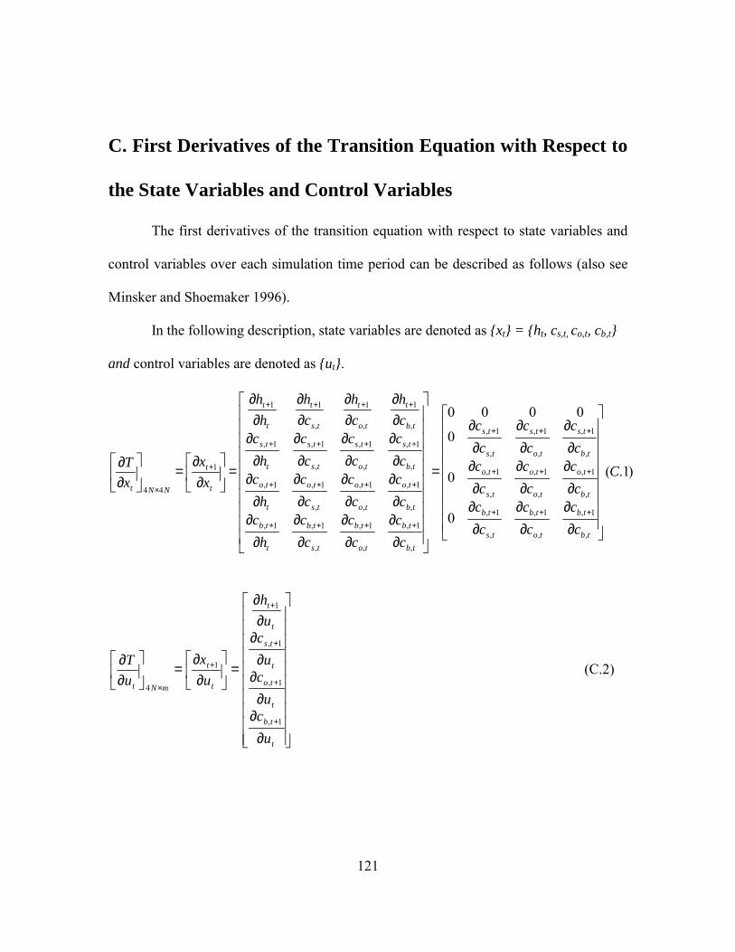
121
C. First Derivatives of the Transition Equation with Respect to
the State Variables and Control Variables
The first derivatives of the transition equation with respect to state variables and
control variables over each simulation time period can be described as follows (also see
Minsker and Shoemaker 1996).
In the following description, state variables are denoted as xt = ht, cs,t, co,t, cb,t
and control variables are denoted as ut.
)1.(
0
0
0
0000
,
1,
,
1,
,
1,
,
1,
,
1,
,
1,
,
1,
,
1,
,
1,
,
1,
,
1,
,
1,1,
,
1,
,
1,
,
1,1,
,
1,
,
1,
,
1,1,
,
1
,
1
,
11
1
44
C
cc
cc
cc
cc
cc
cc
cc
cc
cc
cc
cc
cc
hc
cc
cc
cc
hc
cc
cc
cc
hc
ch
ch
ch
hh
xx
xT
tb
tb
to
tb
ts
tb
tb
to
to
to
ts
to
tb
ts
to
ts
ts
ts
tb
tb
to
tb
ts
tb
t
tb
tb
to
to
to
ts
to
t
to
tb
ts
to
ts
ts
ts
t
ts
tb
t
to
t
ts
t
t
t
t
t
NNt
∂∂
∂∂
∂∂
∂∂
∂∂
∂∂
∂∂
∂∂
∂∂
=
∂∂
∂∂
∂∂
∂∂
∂∂
∂∂
∂∂
∂∂
∂∂
∂∂
∂∂
∂∂
∂∂
∂∂
∂∂
∂∂
=
∂
∂=
∂∂
+++
+++
+++
++++
++++
++++
++++
+
×
∂∂∂
∂∂
∂∂∂
=
∂∂
=
∂∂
+
+
+
+
+
×
t
tb
t
to
t
ts
t
t
t
t
mNt
ucu
cu
cuh
ux
uT
1,
1,
1,
1
1
4
(C.2)
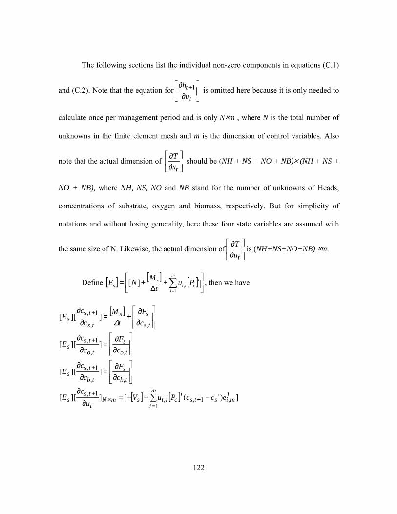
122
The following sections list the individual non-zero components in equations (C.1)
and (C.2). Note that the equation for
∂
∂ +
t
tu
h 1 is omitted here because it is only needed to
calculate once per management period and is only N×m , where N is the total number of
unknowns in the finite element mesh and m is the dimension of control variables. Also
note that the actual dimension of
∂∂
txT should be (NH + NS + NO + NB)× (NH + NS +
NO + NB), where NH, NS, NO and NB stand for the number of unknowns of Heads,
concentrations of substrate, oxygen and biomass, respectively. But for simplicity of
notations and without losing generality, here these four state variables are assumed with
the same size of N. Likewise, the actual dimension of
∂∂
tuT is (NH+NS+NO+NB) ×m.
Define [ ] [ ] [ ]
+∆
+= ∑=
m
i
icit
ss Pu
tMNE
1,][ , then we have
[ ]
[ ] [ ] ])'([]][[
]][[
]][[
]][[
,1,1
,1,
,,
1,
,,
1,
,,
1,
Tmists
m
i
icitsmN
t
tss
tb
s
tb
tss
to
s
to
tss
ts
ss
ts
tss
eccPuVu
cE
cF
cc
E
cF
cc
E
cF
tM
cc
E
−−−=∂
∂
∂∂=
∂∂
∂∂=
∂∂
∂∂+=
∂∂
+=
×+
+
+
+
∑
∆
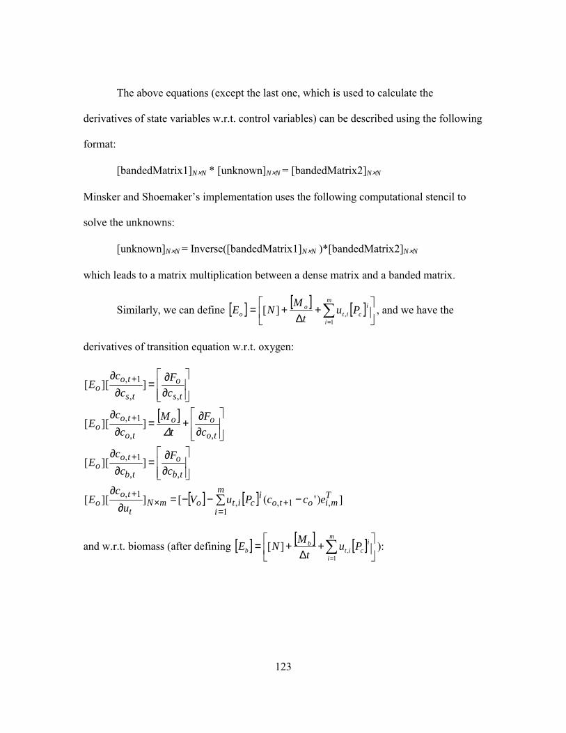
123
The above equations (except the last one, which is used to calculate the
derivatives of state variables w.r.t. control variables) can be described using the following
format:
[bandedMatrix1]N×N * [unknown]N×N = [bandedMatrix2]N×N
Minsker and Shoemakers implementation uses the following computational stencil to
solve the unknowns:
[unknown]N×N = Inverse([bandedMatrix1]N×N )*[bandedMatrix2]N×N
which leads to a matrix multiplication between a dense matrix and a banded matrix.
Similarly, we can define [ ] [ ] [ ]
+∆
+= ∑=
m
i
icit
oo Pu
tMNE
1,][ , and we have the
derivatives of transition equation w.r.t. oxygen:
[ ]
[ ] [ ] ])'([]][[
]][[
]][[
]][[
,1,1
,1,
,,
1,
,,
1,
,,
1,
Tmioto
m
i
icitomN
t
too
tb
o
tb
too
to
oo
to
too
ts
o
ts
too
eccPuVu
cE
cF
cc
E
cF
tM
cc
E
cF
cc
E
−−−=∂
∂
∂∂=
∂∂
∂∂+=
∂∂
∂∂=
∂∂
+=
×+
+
+
+
∑
∆
and w.r.t. biomass (after defining [ ] [ ] [ ]
+∆
+= ∑=
m
i
icit
bb Pu
tMNE
1,][ ):
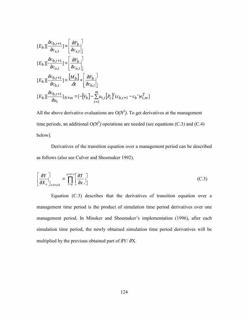
124
[ ]
[ ] [ ] ])'([]][[
]][[
]][[
]][[
,1,1
,1,
,,
1,
,,
1,
,,
1,
Tmibtb
m
i
icitbmN
t
tbb
tb
bb
tb
tbb
to
b
to
tbb
ts
b
ts
tbb
eccPuVu
cE
cF
tM
cc
E
cF
cc
E
cF
cc
E
−−−=∂
∂
∂∂+=
∂∂
∂∂=
∂∂
∂∂=
∂∂
+=
×+
+
+
+
∑
∆
All the above derivative evaluations are O(N3). To get derivatives at the management
time periods, an additional O(N3) operations are needed (see equations (C.3) and (C.4)
below).
Derivatives of the transition equation over a management period can be described
as follows (also see Culver and Shoemaker 1992).
∏−+
=×
∂∂=
∂∂ 1
44
dp
pt tNNk xT
XY (C.3)
Equation (C.3) describes that the derivatives of transition equation over a
management time period is the product of simulation time period derivatives over one
management period. In Minsker and Shoemakers implementation (1996), after each
simulation time period, the newly obtained simulation time period derivatives will be
multiplied by the previous obtained part of ∂Y/ ∂X.
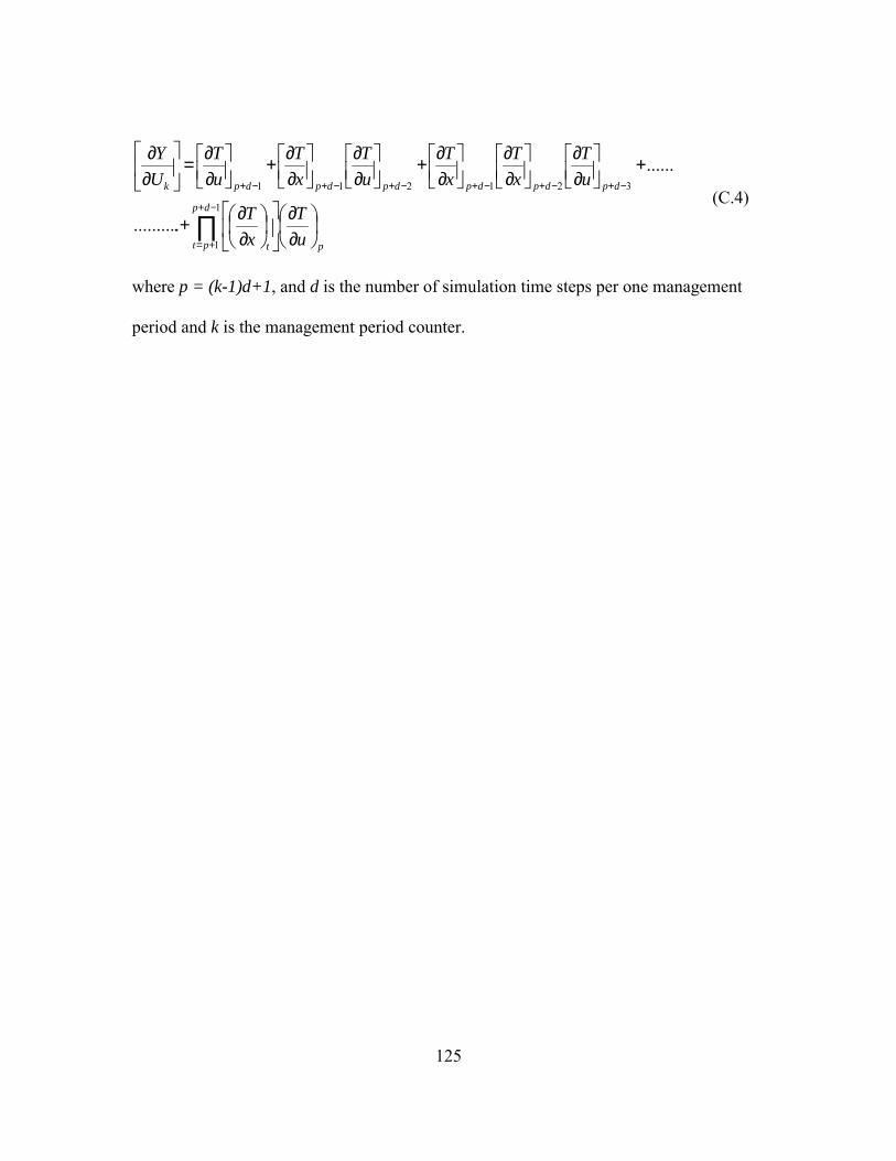
125
p
dp
pt t
dpdpdpdpdpdpk
uT
xT
uT
xT
xT
uT
xT
uT
UY
∂∂
∂∂+
+
∂∂
∂∂
∂∂+
∂∂
∂∂+
∂∂=
∂∂
∏−+
+=
−+−+−+−+−+−+
1
1
321211
...........
......
(C.4)
where p = (k-1)d+1, and d is the number of simulation time steps per one management
period and k is the management period counter.
126
D. Constrained SALQR Method
Constrained SALQR(Successive Approximation Linear Quadratic Regulator )
algorithm with management periods is described in this appendix. Note that the algorithm
given here is only the basic version of SALQR. As the penalty weight increases, penalty
term in Ck matrix (see the definition in the algorithm description) increases and Ck
becomes more and more ill conditioned. To avoid inaccuracy and convergence difficulty,
Liao and Shoemaker (1990) developed a method to partition the matrices A, B, C into A1,
A2, B1, B2, C1, C2. C1 and C2 are inverted separately, which involves QR factorization,
and then "reattached". This advanced version of SALQR is used in the code for this
research but not presented here. See Liao and Shoemaker (1990) for details. Notation is
adapted from Yakowitz and Rutherford (1984), Culver and Shoemaker (1992) and Liao
and Shoemaker (1991). Subscript k indicates management period counters, subscripts x
and u indicate derivatives with respect to X and U, and superscripts T and -1 denote
matrix transpose and inverse, respectively. G indicates the cost function, which has been
augmented by the penalty associated with violating constraints by equation (3) in Chapter
1. The following steps and the flow chart that follows can describe this algorithm.
Step 0: Select a nominal policy kU for k = 1, …, K.
Step 1: Initialize parameters and compute loss and trajectory associated with the given
policy:
(1) set PK+1 = 0NxN, QK+1=01xN, θK+1=0;
127
(2) 1X given and fixed, Xk+1=Y( kX , kU ,k), k=1,…,K;
(3) J(U) = ∑ =Kk kG1 ( kX , kU ,k).
Step 2: Backward sweep: perform the following four procedures recursively, for k =
K,…,1.
1. Compute Ak, Bk, Ck, Dk, Ek, as follows:
Ak = kkTkkxx X
YPXYG )()()(
21
1 ∂∂
∂∂+ +
Bk = kkTkkxu U
YPXYG )()(2)( 1 ∂
∂∂∂+ +
Ck = kkTkkuu U
YPUYG )()()(
21
1 ∂∂
∂∂+ +
Dk = kkk UYQ
UG
)()
( 1 ∂∂+
∂
∂+
Ek = kkk XYQ
XG
)()
( 1 ∂∂+
∂
∂+
2. Compute Pk and Qk according to
kkTkkk BCBAP 1
41 −−=
kkkTkk EBCDQ +−= −1
21
Store Pk and Qk in memory, replacing Pk+1 and Qk+1.
3. Compute αk and βk according to
αk = kk DC 121 −−
128
βk = kk BC 121 −−
and store in memory.
4. Compute
11
21
+− +−= kkk
Tkk DCD θθ
and store θk in place of θk+1.
Step 3: If θ1≤θmin then
kU is the optimal policy;
Otherwise,
Compute the updated control policy as follows:
(1) set ε = 1.0;
(2) compute kU recursively for k = 1,…, K according to the control law:
kU = εαk + βk(Xk- kX ) + kU
Xk+1 = Y( kX , kU ,k)
(3) compute the loss,J:
J(U) = ∑ =Kk kG1 ( kX , kU ,k).
(4) if J(U)-J(U )≤ε(θ1/2),
set kU = kU for k = 1,..,K and
go to Step 1.
Otherwise,
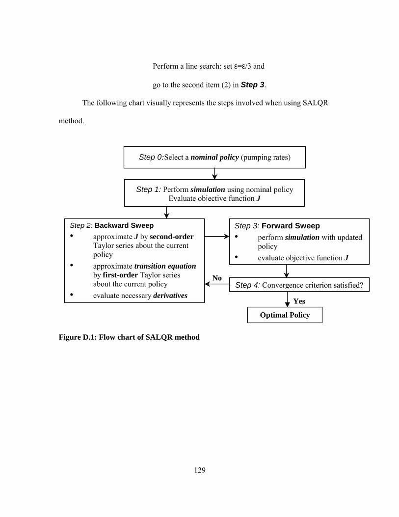
129
Step 0:Select a nominal policy (pumping rates)
Step 1: Perform simulation using nominal policy Evaluate objective function J
Step 2: Backward Sweep approximate J by second-order
Taylor series about the current policy
approximate transition equation by first-order Taylor series about the current policy
evaluate necessary derivatives
Step 3: Forward Sweep perform simulation with updated
policy evaluate objective function J
Step 4: Convergence criterion satisfied?
Yes
No
Optimal Policy
Perform a line search: set ε=ε/3 and
go to the second item (2) in Step 3.
The following chart visually represents the steps involved when using SALQR
method.
Figure D.1: Flow chart of SALQR method
130
References
Ahlfeld, D.P., Mulvey, J.M. and Pinder, G.F.(1986). Designing optimal strategies for
contaminated groundwater remediation, Advances in Water Resources, 9, 77-84.
Ahlfeld, D.P., J.M. Mulvey, G.F. Pinder and E. F. Wood (1988). Contaminated
groundwater remediation design using simulation, optimization, and sensitivity theory.
1. Model development, Water Resour. Res., 24(3), 431-441.
Akian, M., Quadrat, J. P., and Chancelier, J.P. (1988). Dynamic programming complexity
and application, in Proceedings of the 27th IEEE Conference on Decision and Control,
Austin, TX, 1551-1558.
Arian, E., and Taasan, S. (1994a). Multigrid one shot methods for optimal control
problems: infinite dimensional control, ICASE Report No.94-52, Institute for Computer
Applications in Science and Engineering, NASA Langley Research Center, Hampton,
Virginia.
Arian, E., and Ta'asan, S. (1994b). Shape optimization in one shot, in Proceedings of the
Workshop on Optimal Design and Control, Blacksburg, VA, Apr. 8-9, 1994.
(Borggaard, J. et al., eds.), Birkhäuser Boston, Cambridge, MA, 23-40.
131
Arnold, E. and Puta, H. (1994). An SQP-type solution method for constrained discrete-
time optimal control problems. In Computational Optimal Control ed. By R. Bulirsch
and D. Kraft., International Series of Numerical Mathematics, Vol.115. Birkhäuser
Verlag, Switzerland.
Bartholomew-Biggs, M., Brown, S., Christianson, B., and Dixon, L. (2000). Automatic
differentiation of algorithms, Journal of Computational and Applied Mathematics,
124(1-2), 171-190.
Bear, J., and Sun, Y.(1998). Optimization of Pump-Treat-Inject (PTI) design for the
remediation of a contaminated aquifer: multi-stage design with chance-constraints, J. of
Contaminant Hydrology, 29(3): 223-242.
Beckie, R., Wood, E. F., and Aldama, A. A. (1993). Mixed finite element simulation of
saturated groundwater flow using a multigrid accelerated domain decomposition
technique, Water Resour. Res., 29(9), 3145-3157.
Biros, G., and Ghattas, O. (2000). A Lagrange-Newton-Krylov-Schur method for PDE-
constrained optimization, SIAG/OPT Views-and-News, 11(2), August 2000.
Biros, G. and Ghatta, O. (1999). Parallel Newton-Krylov methods for PDE-constrained
optimization, In Proceedings of SC’99, November 13-19, 1999, Portland, OR.
Boggs, P.T., and Tolle, J. W. (2000). Sequential quadratic programming for large-scale
nonlinear optimization, Journal of Computational and Applied Mathematics, 124(1-2),
123-137.
Brandt, A. (1977). Multi-level adaptive solutions to boundary-value problems, Math.
Comp., 31, 333-390.
132
Brandt, A.(1997). The Gauss center research in multiscale scientific computation,
Electronic Transactions on Numerical Analysis, 6, 1-34.
Brandt, A. (2001). Multiscale Scientific Computation: Review 2000. Copper Mountain
Conferences on Multigrid Methods, Copper Mountain, CO., April 1-6, 2001,
(http://www.mgnet.org/mgnet-cm2001.html).
Briggs, W.L.(1987). A Multigrid Tutorial, SIAM, Philadelphia.
Carriaga, C.C., and Mays, L.W.(1995). Optimal control approach for sedimentation
control in alluvial rivers, J. Water Resour. Plan. Manage., 121(6), 408-417.
Chang, L.-C., Shoemaker, C.A., and Liu, P. L.-F. (1992). Optimal time-varying pumping
rates for groundwater remediation: application of a constrained optimal control
algorithm, Water Resour. Res., 28(12), 3157-3173.
Cheng, H.-P., Yeh, G.-T., Xu, J., Li, M.-H., and Carsel, R. (1998). A study of
incorporating the multigrid method into the three-dimensional finite element
discretization: a modular setting and application, International Journal for Numerical
Methods in Engineering, 41(3), 499-526.
Chow, C.-S., and Tsitsiklis, J.N. (1991). An optimal one-way multigrid algorithm for
discrete-time stochastic control, IEEE Transactions on Automatic Control, 36(8), 898-
914.
Christianson, B., and Bartholomew-Biggs, M.(2000). Generalization of Pantojas optimal
control algorithm, The 3rd International Conference/Workshop on Automatic
Differentiation: From Simulation to Optimization, June 19-23, 2000, Maison du
Séminaire, Nice, France.
133
Culver, T.B., and Shoemaker, C.A. (1992). Dynamic optimal control for groundwater
remediation with flexible management periods, Water Resour. Res., 28(3), 629-641.
Culver, T.B., and Shoemaker, C.A. (1993). Optimal control for groundwater remediation
by differential dynamic programming with quasi-Newton, Water Resour. Res., 29(4),
823-831.
Douglas, C. C.(1984). Multi-Grid algorithms with applications to elliptic boundary-value
problems, SIAM J. Numer. Anal., 21(2), 236-254.
Douglas,C.C.(1996). Multigrid methods in science and engineering, IEEE Computational
Science & Engineering, 3(4), pp.55-68.
Dunn, J.C., and Bertsekas, P.B.(1989). Efficient Dynamic Programming Implementations
of Newton's Method for Unconstrained Optimal Control Problems. Journal of
Optimization Theory and Applications, 63(1), 23-38.
Dreyer, T., Maar, B., and Schulz, V. (2000). Multigrid optimization in applications,
Journal of Computational and Applied Mathematics, 120(1-2), 67-84.
EPA (Environmental Protection Agency). (1997). Cleaning Up the Nation’s Waste Sites:
Markets and Technology Trends. EPA 542-R-96-005. Washington, D.C.: EPA, Office
of Solid Waste and Emergency Response.
Ferraresi, M., Todini, E., and Vignoli, R. (1996). A solution to the inverse problem in
groundwater hydrology based on Kalman filtering, Journal of Hydrology. 175(1-4),
567-572.
Gelhar, L.W., Welty, C. and Rehfeldt, K. R. (1992). A critical review data on field-scale
dispersion in aquifers, Water Resour. Res., 28(7), 1955-1974.
134
Gorelick, S.M., Voss, C.I., Gill, P.E., Murray, W., Saunders, M.A. and Wright,
M.H.(1984). Aquifer reclamation design: the use of contaminant transport simulation
combined with nonlinear programming, Water Resour. Res., 20(4), 415-427.
Graham, W.D., and McLaughlin, D.B. (1991). A stochastic model of solute transport in
groundwater: application to the Borden, Ontario, tracer test, Water Resour. Res., 27(6),
1345-1359.
Hackbusch, W.(1979). On the fast solving of parabolic boundary control problems, SIAM
J. Control and Optimization, 17(2), 231-244.
Hackbusch, W.(1985). Multi-grid Methods and Applications, Springer-Verlag, Berlin.
Hoppe, R.H.W.(1986). Multi-grid methods for Hamilton-Jacobi-Bellman equations,
Numerische Mathematik, 49, 239-254.
Hovland, P. D., Keyes, D. E., McInnes, L. C., and Samyono, W. (2000). Using automatic
differentiation for second-order matrix-free methods in PDE-constrained optimization,
Preprint ANL/MCS-P855-1100, Mathematics and Computer Science Division, Argonne
National Laboratory.
Huang, C. and Mayer, A. S.(1997). Pump-and-treat optimization using well locations and
pumping rates as decision variables. Water Resour. Res., 33(5), 1001-1012.
Iserles, A.(1996). A First Course in the Numerical Analysis of Differential Equations.
Cambridge University Press, New York.
Jones, L., Willis, R., and Yeh, W. W-G (1987). Optimal control of nonlinear groundwater
hydraulics using differential dynamic programming, Water Resour. Res., 23(11), 2097-
2106.
135
Jones, J.E., and Woodward C.S.(2001). Newton-Krylov-multigrid solvers for large-scale,
highly heterogeneous, variably saturated flow problems, Advances in Water Resources,
24(7), 763-774.
Joppich, W., and Mijalković, S. (1993). Multigrid Methods for Process Simulation,
Springer-Verlag /Wien, New York.
Kronsjö, L., and Dahlquist, G. (1971). On the design of nested iterations for elliptic
difference equations, BIT, 11,63-71.
Lewis, R. M., and Nash, S.G.,(2000) A multigrid approach to the optimization of systems
governed by differential equations. In Proceedings of the 8th AIAA/USAF/NASA/ISSMO
Symposium on Multidisciplinary Analysis and Optimization, Sept.6-8, 2000, Long
Beach, CA.
Li, G., and Mays, L.W. (1995). Differential dynamic programming for estuarine
management, J. Water Resour. Plan. Manage., 121(6), 455-462.
Li, M.-H., Cheng, H.-P., and Yeh, G.-T. (2000). Solving 3D subsurface flow and
transport with adaptive multigrid, Journal of Hydrologic Engineering, 5(1), 74-81.
Liao, L.-Z., and Shoemaker, C.A (1990). Constrained differential partitioning and QR
factorization to avoid numerical ill-conditioning of penalty function for constrained
nonlinear programming and control, Proc. IEEE Conf. on Decision and Control,
Honolulu, Hawaii.
Liao, L.-Z., and Shoemaker, C.A. (1991). Convergence in unconstrained discrete-time
differential dynamic programming, IEEE Trans. Autom. Control, 36, 692-706.
136
Liu,Y., Minsker, B.S., and Saied, F.(2001). A one-way spatial multiscale method for
optimal bioremediation design, J. Water Resour. Plan. Manage.,127 (2), 130-139.
Liu, Y. and Minsker, B.S. (2001, in press). Efficient multiscale methods for optimal in-
situ bioremediation design, J. Water Resour. Plan. Manage. , in press.
Mackay, D.M., Freyberg, D.L., and Roberts, P.V. (1986). A natural gradient experiment
on solute transport in a sand aquifer 1. approach and overview of plume movement,
Water Resour. Res., 22(13), 2017-2029.
Mansfield, C. M. and Shoemaker, C. A.(1999). Optimal remediation of unconfined
aquifers: Numerical applications and derivative calculations, Water Resour. Res.,
35(5), 1455-1470.
Mansfield, C. M., Shoemaker, C. A., and Liao, L-Z. (1998). Utilizing sparsity in time-
varying optimal control of aquifer cleanup, J. Water Resour. Plan. Manage., 124(1),
39-46.
Maar, B., and Schulz, V. (2000). Interior point multigrid methods for topology
optimization, Struct. Multidisc. Optim., 19(3), 214-224.
Mavriplis, D.J., and Jameson, A. (1990). Multigrid solution of the navier-stokes
equations on triangular meshes, AIAA JOURNAL, 28(8), 1415-1425.
Mckeon, T. J., and Chu, W. (1987). A multigrid model for steady flow in partially
saturated porous media, Water Resour. Res., 23(4), 542-550.
McLaughlin, D., and Townley, L. R. (1996). A reassessment of the groundwater inverse
problem, Water Resour. Res., 32(5), 1131-1162.
137
Merckx, C. (1991). Optimal pumping strategy for groundwater decontamination, Int. J.
Control, 53(4), 889-905.
Migdalas, A., Pardalos, P. M., and Värbrand, P. (1998). Multilevel Optimization:
Algorithms and Applications, Kluwer Academic Publishers, Netherlands.
Minsker, B. S., and Shoemaker, C. A. (1996). Differential a finite element biodegradation
simulation model for optimal control. Water Resour. Res., 32(1),187-192.
Minsker, B. S., and Shoemaker, C.A. (1998a). Computational issues for optimal in-situ
bioremediation design, J. Water Resour. Plan. Manage., 124(1), 39-46.
Minsker, B. S., and Shoemaker, C.A. (1998b). Dynamic optimal control of in-situ
bioremediation of groundwater, J. Water Resour. Plan. Manage., 124(3), 149-161.
Mjolsness, E., Garrett, C.D., and Miranker, W.L. (1991). Multiscale optimization in
neural nets, IEEE Transactions on Neural Networks, 2(2), 263-274.
Murray, D.M., and Yakowitz, S.J. (1979). Constrained differential dynamic programming
and its application to multireservoir control, Water Resour. Res., 15(5),1017-1027.
Murray, D.M., and Yakowitz, S.J. (1984). Differential Dynamic Programming and
Newton's Method for Discrete Optimal Control Problems. Journal of Optimization
Theory and Applications, 43(3), 395-414.
Nash, S.G. (2000). A multigrid approach to discretized optimization problems,
Optimization Methods & Software, 1(8), 1-18.
National Research Council (1994). Alternatives for Ground Water Cleanup, National
Academy Press, Washington, D.C..
138
Pantoja, J.F.A. De O. (1988). Differential Dynamic Programming and Newton's Method.
Int. J. Control, 47(5), 1539-1553.
Russell, M., Colglazier, E. W., and English, M.R. (1991). Hazardous Waste Remediation:
The Task Ahead. Knoxville: University of Tennessee, Waste Management Research and
Education Institute.
Saied, F. S., and Mahinthakumar, G. (1998). Efficient parallel multigrid based solvers
for large-scale groundwater flow simulations, Computers Math. Applic., 35(7), 45-54.
Schulz, V., Bardossy, A., and Helmig, R.(1999). Conditional statistical inverse modeling
in groundwater flow by multigrid methods, Computational Geosciences, 3(1), 49-68.
Stüben, K., and Trottenberg, U. (1982). Fundamental algorithms, model problem analysis
and applications, Multigrid Methods, edited by W. Hackbusch and U. Trottenberg,
Lecture Notes in Mathematics, Vol. 960, 1-176.
Taasan, S.(1991). One Shot methods for optimal control of distributed parameter
systems I: finite dimensional control, ICASE Report No.91-2, Institute for Computer
Applications in Science and Engineering, NASA Langley Research Center, Hampton,
Virginia.
Whiffen, G.J., and Shoemaker, C.A. (1993). Nonlinear weighted feedback control of
groundwater remediation under uncertainty, Water Resour. Res., 29, 3277-3289.
Whiffen, G.J.(1995). Optimal control for deterministic and uncertain groundwater
remediation, Ph.D. thesis, School of Civil and Environmental Engineering, Cornell
Univ., Ithaca, New York.
139
Woodbury, A. D., and Ulrych, T. J. (2000). A full-Bayesian approach to the groundwater
inverse problem for steady state flow, Water Resour. Res., 36(8), 2081-2094.
Yakowitz, S., and Rutherford, B. (1984). Computational aspects of discrete-time optimal
control, Applied Mathematics and Computation, 15, 29-45.
Yoon, J.-H., and Shoemaker, C.A. (1999). Comparison of optimization methods for
ground-water bioremediation, J. Water Resour. Plan. Manage., 125(1), 54-63.
Zio, E. (1997). Approaching the inverse problem of parameter estimation in groundwater
models by means of artificial neural networks. Progress in Nuclear Energy. 31(3), 303-
315.
140
Vita
Yong Liu received his Bachelor of Engineering and Master of Engineering
degrees, both in Environmental Engineering, from Tsinghua University, Beijing, China,
in 1994 and 1997, receptively. During his graduate study from 1994 to 1997 in Tsinghua
University, he developed a regional environmental resources and information system
using technologies from geographic information system, remote sensing and management
information systems. He was also a member of the research and development team for
Chinas provincial level environmental information systems from 1994 to 1996, where he
was responsible for the database schema design and system analysis. In August 1997, he
was admitted to the Ph.D. program in Civil and Environmental Engineering at the
University of Illinois at Urbana-Champaign. He held one-year Computational Science
and Engineering fellowship from 1997 to 1998. He received his Master of Computer
Science degree from the University of Illinois at Urbana-Champaign in May 2001. His
interests include groundwater remediation design, PDE-constrained optimization,
environmental information technology, and computational informatics.