Embed Size (px)
Citation preview
www.dbeBooks.com - An Ebook Library

The Art of Error Correcting Coding
The Art of Error Correcting Coding, Second Edition Robert H. Morelos-Zaragoza 2006 John Wiley & Sons, Ltd. ISBN: 0-470-01558-6
The Art of Error Correcting Coding
Second Edition
Robert H. Morelos-ZaragozaSan Jose State University, USA

Copyright 2006 John Wiley & Sons Ltd, The Atrium, Southern Gate, Chichester,West Sussex PO19 8SQ, England
Telephone (+44) 1243 779777
Email (for orders and customer service enquiries): [email protected] our Home Page on www.wiley.com
All Rights Reserved. No part of this publication may be reproduced, stored in a retrieval system or transmittedin any form or by any means, electronic, mechanical, photocopying, recording, scanning or otherwise, exceptunder the terms of the Copyright, Designs and Patents Act 1988 or under the terms of a licence issued by theCopyright Licensing Agency Ltd, 90 Tottenham Court Road, London W1T 4LP, UK, without the permission inwriting of the Publisher. Requests to the Publisher should be addressed to the Permissions Department, JohnWiley & Sons Ltd, The Atrium, Southern Gate, Chichester, West Sussex PO19 8SQ, England, or emailed [email protected], or faxed to (+44) 1243 770620.
Designations used by companies to distinguish their products are often claimed as trademarks. All brand namesand product names used in this book are trade names, service marks, trademarks or registered trademarks oftheir respective owners. The Publisher is not associated with any product or vendor mentioned in this book.
This publication is designed to provide accurate and authoritative information in regard to the subject mattercovered. It is sold on the understanding that the Publisher is not engaged in rendering professional services. Ifprofessional advice or other expert assistance is required, the services of a competent professional should besought.
Other Wiley Editorial Offices
John Wiley & Sons Inc., 111 River Street, Hoboken, NJ 07030, USA
Jossey-Bass, 989 Market Street, San Francisco, CA 94103-1741, USA
Wiley-VCH Verlag GmbH, Boschstr. 12, D-69469 Weinheim, Germany
John Wiley & Sons Australia Ltd, 42 McDougall Street, Milton, Queensland 4064, Australia
John Wiley & Sons (Asia) Pte Ltd, 2 Clementi Loop #02-01, Jin Xing Distripark, Singapore 129809
John Wiley & Sons Canada Ltd, 6045 Freemont Blvd, Mississauga, ONT, L5R 4J3, Canada
Wiley also publishes its books in a variety of electronic formats. Some content that appearsin print may not be available in electronic books.
British Library Cataloguing in Publication Data
A catalogue record for this book is available from the British Library
ISBN-13: 978-0-470-01558-2 (HB)ISBN-10: 0-470-01558-6 (HB)
Typeset in 10/12pt Times by Laserwords Private Limited, Chennai, India.Printed and bound in Great Britain by Antony Rowe Ltd, Chippenham, England.This book is printed on acid-free paper responsibly manufactured from sustainable forestryin which at least two trees are planted for each one used for paper production.
Contents
Preface ix
Foreword xi
The ECC web site xiii
1 Introduction 11.1 Error correcting coding: Basic concepts . . . . . . . . . . . . . . . . . . . . 4
1.1.1 Block codes and convolutional codes . . . . . . . . . . . . . . . . . 41.1.2 Hamming distance, Hamming spheres and error correcting capability 5
1.2 Linear block codes . . . . . . . . . . . . . . . . . . . . . . . . . . . . . . . 71.2.1 Generator and parity-check matrices . . . . . . . . . . . . . . . . . 71.2.2 The weight is the distance . . . . . . . . . . . . . . . . . . . . . . . 8
1.3 Encoding and decoding of linear block codes . . . . . . . . . . . . . . . . . 81.3.1 Encoding with G and H . . . . . . . . . . . . . . . . . . . . . . . . 81.3.2 Standard array decoding . . . . . . . . . . . . . . . . . . . . . . . . 101.3.3 Hamming spheres, decoding regions and the standard array . . . . . 12
1.4 Weight distribution and error performance . . . . . . . . . . . . . . . . . . 131.4.1 Weight distribution and undetected error probability over a BSC . . 141.4.2 Performance bounds over BSC, AWGN and fading channels . . . . 15
1.5 General structure of a hard-decision decoder of linear codes . . . . . . . . . 23Problems . . . . . . . . . . . . . . . . . . . . . . . . . . . . . . . . . . . . . . . 23
2 Hamming, Golay and Reed–Muller codes 272.1 Hamming codes . . . . . . . . . . . . . . . . . . . . . . . . . . . . . . . . . 27
2.1.1 Encoding and decoding procedures . . . . . . . . . . . . . . . . . . 282.2 The binary Golay code . . . . . . . . . . . . . . . . . . . . . . . . . . . . . 29
2.2.1 Encoding . . . . . . . . . . . . . . . . . . . . . . . . . . . . . . . . 292.2.2 Decoding . . . . . . . . . . . . . . . . . . . . . . . . . . . . . . . . 302.2.3 Arithmetic decoding of the extended (24, 12, 8) Golay code . . . . 30
2.3 Binary Reed–Muller codes . . . . . . . . . . . . . . . . . . . . . . . . . . . 312.3.1 Boolean polynomials and RM codes . . . . . . . . . . . . . . . . . 312.3.2 Finite geometries and majority-logic decoding . . . . . . . . . . . . 33
Problems . . . . . . . . . . . . . . . . . . . . . . . . . . . . . . . . . . . . . . . 37
vi CONTENTS
3 Binary cyclic codes and BCH codes 393.1 Binary cyclic codes . . . . . . . . . . . . . . . . . . . . . . . . . . . . . . . 39
3.1.1 Generator and parity-check polynomials . . . . . . . . . . . . . . . 393.1.2 The generator polynomial . . . . . . . . . . . . . . . . . . . . . . . 403.1.3 Encoding and decoding of binary cyclic codes . . . . . . . . . . . . 413.1.4 The parity-check polynomial . . . . . . . . . . . . . . . . . . . . . 423.1.5 Shortened cyclic codes and CRC codes . . . . . . . . . . . . . . . . 443.1.6 Fire codes . . . . . . . . . . . . . . . . . . . . . . . . . . . . . . . . 45
3.2 General decoding of cyclic codes . . . . . . . . . . . . . . . . . . . . . . . 463.2.1 GF(2m) arithmetic . . . . . . . . . . . . . . . . . . . . . . . . . . . 48
3.3 Binary BCH codes . . . . . . . . . . . . . . . . . . . . . . . . . . . . . . . 523.3.1 BCH bound . . . . . . . . . . . . . . . . . . . . . . . . . . . . . . . 53
3.4 Polynomial codes . . . . . . . . . . . . . . . . . . . . . . . . . . . . . . . . 533.5 Decoding of binary BCH codes . . . . . . . . . . . . . . . . . . . . . . . . 54
3.5.1 General decoding algorithm for BCH codes . . . . . . . . . . . . . 563.5.2 The Berlekamp–Massey algorithm (BMA) . . . . . . . . . . . . . . 573.5.3 PGZ decoder . . . . . . . . . . . . . . . . . . . . . . . . . . . . . . 603.5.4 Euclidean algorithm . . . . . . . . . . . . . . . . . . . . . . . . . . 613.5.5 Chien search and error correction . . . . . . . . . . . . . . . . . . . 633.5.6 Errors-and-erasures decoding . . . . . . . . . . . . . . . . . . . . . 63
3.6 Weight distribution and performance bounds . . . . . . . . . . . . . . . . . 653.6.1 Error performance evaluation . . . . . . . . . . . . . . . . . . . . . 66
Problems . . . . . . . . . . . . . . . . . . . . . . . . . . . . . . . . . . . . . . . 69
4 Nonbinary BCH codes: Reed–Solomon codes 734.1 RS codes as polynomial codes . . . . . . . . . . . . . . . . . . . . . . . . . 734.2 From binary BCH to RS codes . . . . . . . . . . . . . . . . . . . . . . . . 734.3 Decoding RS codes . . . . . . . . . . . . . . . . . . . . . . . . . . . . . . . 74
4.3.1 Remarks on decoding algorithms . . . . . . . . . . . . . . . . . . . 794.3.2 Errors-and-erasures decoding . . . . . . . . . . . . . . . . . . . . . 79
4.4 Weight distribution . . . . . . . . . . . . . . . . . . . . . . . . . . . . . . . 84Problems . . . . . . . . . . . . . . . . . . . . . . . . . . . . . . . . . . . . . . . 84
5 Binary convolutional codes 875.1 Basic structure . . . . . . . . . . . . . . . . . . . . . . . . . . . . . . . . . 87
5.1.1 Recursive systematic convolutional codes . . . . . . . . . . . . . . . 925.1.2 Free distance . . . . . . . . . . . . . . . . . . . . . . . . . . . . . . 94
5.2 Connections with block codes . . . . . . . . . . . . . . . . . . . . . . . . . 945.2.1 Zero-tail construction . . . . . . . . . . . . . . . . . . . . . . . . . 945.2.2 Direct-truncation construction . . . . . . . . . . . . . . . . . . . . . 955.2.3 Tail-biting construction . . . . . . . . . . . . . . . . . . . . . . . . . 955.2.4 Weight distributions . . . . . . . . . . . . . . . . . . . . . . . . . . 95
5.3 Weight enumeration . . . . . . . . . . . . . . . . . . . . . . . . . . . . . . . 975.4 Performance bounds . . . . . . . . . . . . . . . . . . . . . . . . . . . . . . 995.5 Decoding: Viterbi algorithm with Hamming metrics . . . . . . . . . . . . . 101
5.5.1 Maximum-likelihood decoding and metrics . . . . . . . . . . . . . . 101
CONTENTS vii
5.5.2 The Viterbi algorithm . . . . . . . . . . . . . . . . . . . . . . . . . 1025.5.3 Implementation issues . . . . . . . . . . . . . . . . . . . . . . . . . 104
5.6 Punctured convolutional codes . . . . . . . . . . . . . . . . . . . . . . . . . 1125.6.1 Implementation issues related to punctured convolutional codes . . . 1155.6.2 RCPC codes . . . . . . . . . . . . . . . . . . . . . . . . . . . . . . 116
Problems . . . . . . . . . . . . . . . . . . . . . . . . . . . . . . . . . . . . . . . 116
6 Modifying and combining codes 1196.1 Modifying codes . . . . . . . . . . . . . . . . . . . . . . . . . . . . . . . . 119
6.1.1 Shortening . . . . . . . . . . . . . . . . . . . . . . . . . . . . . . . 1196.1.2 Extending . . . . . . . . . . . . . . . . . . . . . . . . . . . . . . . . 1216.1.3 Puncturing . . . . . . . . . . . . . . . . . . . . . . . . . . . . . . . 1226.1.4 Augmenting, expurgating and lengthening . . . . . . . . . . . . . . 122
6.2 Combining codes . . . . . . . . . . . . . . . . . . . . . . . . . . . . . . . . 1246.2.1 Time sharing of codes . . . . . . . . . . . . . . . . . . . . . . . . . 1246.2.2 Direct sums of codes . . . . . . . . . . . . . . . . . . . . . . . . . . 1256.2.3 The |u|u + v|-construction and related techniques . . . . . . . . . . 1266.2.4 Products of codes . . . . . . . . . . . . . . . . . . . . . . . . . . . 1286.2.5 Concatenated codes . . . . . . . . . . . . . . . . . . . . . . . . . . 1346.2.6 Generalized concatenated codes . . . . . . . . . . . . . . . . . . . . 136
Problems . . . . . . . . . . . . . . . . . . . . . . . . . . . . . . . . . . . . . . . 140
7 Soft-decision decoding 1437.1 Binary transmission over AWGN channels . . . . . . . . . . . . . . . . . . 1447.2 Viterbi algorithm with Euclidean metric . . . . . . . . . . . . . . . . . . . . 1457.3 Decoding binary linear block codes with a trellis . . . . . . . . . . . . . . . 1467.4 The Chase algorithm . . . . . . . . . . . . . . . . . . . . . . . . . . . . . . 1507.5 Ordered statistics decoding . . . . . . . . . . . . . . . . . . . . . . . . . . . 1537.6 Generalized minimum distance decoding . . . . . . . . . . . . . . . . . . . 156
7.6.1 Sufficient conditions for optimality . . . . . . . . . . . . . . . . . . 1577.7 List decoding . . . . . . . . . . . . . . . . . . . . . . . . . . . . . . . . . . 1587.8 Soft-output algorithms . . . . . . . . . . . . . . . . . . . . . . . . . . . . . 158
7.8.1 Soft-output Viterbi algorithm . . . . . . . . . . . . . . . . . . . . . 1587.8.2 Maximum-a posteriori (MAP) algorithm . . . . . . . . . . . . . . . 1617.8.3 Log-MAP algorithm . . . . . . . . . . . . . . . . . . . . . . . . . . 1637.8.4 Max-Log-MAP algorithm . . . . . . . . . . . . . . . . . . . . . . . 1647.8.5 Soft-output OSD algorithm . . . . . . . . . . . . . . . . . . . . . . 164
Problems . . . . . . . . . . . . . . . . . . . . . . . . . . . . . . . . . . . . . . . 165
8 Iteratively decodable codes 1698.1 Iterative decoding . . . . . . . . . . . . . . . . . . . . . . . . . . . . . . . . 1728.2 Product codes . . . . . . . . . . . . . . . . . . . . . . . . . . . . . . . . . . 174
8.2.1 Parallel concatenation: Turbo codes . . . . . . . . . . . . . . . . . . 1748.2.2 Serial concatenation . . . . . . . . . . . . . . . . . . . . . . . . . . 1838.2.3 Block product codes . . . . . . . . . . . . . . . . . . . . . . . . . . 185
8.3 Low-density parity-check codes . . . . . . . . . . . . . . . . . . . . . . . . 1908.3.1 Tanner graphs . . . . . . . . . . . . . . . . . . . . . . . . . . . . . 190
viii CONTENTS
8.3.2 Iterative hard-decision decoding: The bit-flip algorithm . . . . . . . 1928.3.3 Iterative probabilistic decoding: Belief propagation . . . . . . . . . 196
Problems . . . . . . . . . . . . . . . . . . . . . . . . . . . . . . . . . . . . . . . 201
9 Combining codes and digital modulation 2039.1 Motivation . . . . . . . . . . . . . . . . . . . . . . . . . . . . . . . . . . . . 203
9.1.1 Examples of signal sets . . . . . . . . . . . . . . . . . . . . . . . . 2049.1.2 Coded modulation . . . . . . . . . . . . . . . . . . . . . . . . . . . 2069.1.3 Distance considerations . . . . . . . . . . . . . . . . . . . . . . . . 207
9.2 Trellis-coded modulation (TCM) . . . . . . . . . . . . . . . . . . . . . . . . 2089.2.1 Set partitioning and trellis mapping . . . . . . . . . . . . . . . . . . 2099.2.2 Maximum-likelihood decoding . . . . . . . . . . . . . . . . . . . . 2119.2.3 Distance considerations and error performance . . . . . . . . . . . . 2129.2.4 Pragmatic TCM and two-stage decoding . . . . . . . . . . . . . . . 213
9.3 Multilevel coded modulation . . . . . . . . . . . . . . . . . . . . . . . . . . 2179.3.1 Constructions and multistage decoding . . . . . . . . . . . . . . . . 2179.3.2 Unequal error protection with MCM . . . . . . . . . . . . . . . . . 221
9.4 Bit-interleaved coded modulation . . . . . . . . . . . . . . . . . . . . . . . 2259.4.1 Gray mapping . . . . . . . . . . . . . . . . . . . . . . . . . . . . . 2269.4.2 Metric generation: De-mapping . . . . . . . . . . . . . . . . . . . . 2279.4.3 Interleaving . . . . . . . . . . . . . . . . . . . . . . . . . . . . . . . 227
9.5 Turbo trellis-coded modulation . . . . . . . . . . . . . . . . . . . . . . . . . 2279.5.1 Pragmatic turbo TCM . . . . . . . . . . . . . . . . . . . . . . . . . 2289.5.2 Turbo TCM with symbol interleaving . . . . . . . . . . . . . . . . . 2289.5.3 Turbo TCM with bit interleaving . . . . . . . . . . . . . . . . . . . 229
Problems . . . . . . . . . . . . . . . . . . . . . . . . . . . . . . . . . . . . . . . 230
Appendix A Weight distributions of extended BCH codes 233A.1 Length 8 . . . . . . . . . . . . . . . . . . . . . . . . . . . . . . . . . . . . . 233A.2 Length 16 . . . . . . . . . . . . . . . . . . . . . . . . . . . . . . . . . . . . 233A.3 Length 32 . . . . . . . . . . . . . . . . . . . . . . . . . . . . . . . . . . . . 234A.4 Length 64 . . . . . . . . . . . . . . . . . . . . . . . . . . . . . . . . . . . . 235A.5 Length 128 . . . . . . . . . . . . . . . . . . . . . . . . . . . . . . . . . . . 238
Bibliography 247
Index 257
Preface
The first edition of this book was the result of hundreds of emails from all over theworld with questions on the theory and applications of error correcting coding (ECC),from colleagues from both academia and industry. Most of the questions have been fromengineers and computer scientists needing to select, implement or simulate a particularcoding scheme. The questions were sparked by a popular web site1 initially set up at ImaiLaboratory at the Institute of Industrial Science, University of Tokyo, in early 1995. Animportant aspect of this text is the absence of theorems and proofs. The approach is toteach basic concepts using simple examples. References to theoretical developments aremade when needed. This book is intended to be a reference guide to error correctingcoding techniques for graduate students and professionals interested in learning the basictechniques and applications of ECC. Computer programs that implement the basic encodingand decoding algorithms of practical coding schemes are available on a companion website. This site is referred to as the “ECC web site” throughout the text and is located at:
http://the-art-of-ecc.com
This book is unique in that it introduces the basic concepts of error correcting codes withsimple illustrative examples. Computer programs written in C language and new Matlab2
scripts are available on the ECC web site and help illustrate the implementation of basicencoding and decoding algorithms of important coding schemes, such as convolutionalcodes, Hamming codes, BCH codes, Reed–Solomon codes and turbo codes, and theirapplication in digital communication systems. There is a rich theory of ECC that will betouched upon, by referring to the appropriate material. There are many good books dealingwith the theory of ECC, for example, references (Lin and Costello 2005), (MacWilliamsand Sloane 1977), (Peterson and Weldon 1972), (Blahut 1984), (Bossert 1999), (Wicker1995), just to cite a few. Readers may wish to consult them before, during or after goingthrough the material in this book. Each chapter describes, using simple and easy-to-follownumerical examples, the basic concepts of a particular coding or decoding scheme, ratherthan going into the detail of the theory behind it. Basic analysis tools are given to help inthe assessment of the error performance of a particular ECC scheme.
The book deals with the art of error correcting coding, in the sense that it addresses theneed for selecting, implementing and simulating algorithms for encoding and decoding ofcodes for error correction and detection. New features of the second edition include addi-tional in-text examples as well as new problems at the end of each chapter, intended foruse in a course on ECC. A comprehensive bibliography is included, for readers who wish
1http://www.eccpage.com2Matlab is a registered trademark of The Mathworks, Inc.
x PREFACE
to learn more about the beautiful theory that makes it all work. The book is organized asfollows. In Chapter 1, the basic concepts of error correction and coding and decoding tech-niques are introduced. Chapter 2 deals with important and simple-to-understand families ofcodes, such as the Hamming, Golay and Reed–Muller codes. In Chapter 3, cyclic codes andthe important family of BCH codes are described. Finite-field arithmetic is introduced andbasic decoding algorithms, such as Berlekamp–Massey, Euclidean and PGZ, are described,and easy to follow examples are given to understand their operation. Chapter 4 deals withReed–Solomon codes and errors-and-erasures decoding. A comprehensive treatment of theavailable algorithms is given, along with examples of their operation. In Chapter 5, binaryconvolutional codes are introduced. Focus in this chapter is on the understanding of thebasic structure of these codes, along with a basic explanation of the Viterbi algorithm withHamming metrics. Important implementation issues are discussed. In Chapter 6, severaltechniques for modifying a single code or combining several codes are given and illus-trated by simple examples. Chapter 7 deals with soft-decision decoding algorithms, someof which have not yet received attention in the literature, such as a soft-output ordered-statistics decoding algorithm. Moreover, Chapter 8 presents a unique treatment of turbocodes, both parallel concatenated and serial concatenated, and block product codes, froma coding theoretical perspective. In the same chapter, low-density parity-check codes areexamined. For all these classes of codes, basic decoding algorithms are described and sim-ple examples are given. Finally, Chapter 9 deals with powerful techniques that combineerror correcting coding with digital modulation, and several clever decoding techniques aredescribed.
I would like to express my gratitude to the following persons for inspiring this work.Professor Francisco Garcia Ugalde, Universidad Nacional Autonoma de Mexico, for intro-ducing me to the exciting world of error correcting codes. Parts of this book are based on myBachelor’s thesis under his direction. Professor Edward Bertram, University of Hawaii, forteaching me the basics of abstract algebra. Professor David Munoz, Instituto Technologicoy de Estudios Superiores de Monterrey, Mexico, for his kindness and support. ProfessorsTadao Kasami, Hiroshima City University, Toru Fujiwara, University of Osaka, and HidekiImai, University of Tokyo, for supporting my stay as a visiting academic researcher inJapan. Dan Luthi and Advait Mogre, LSI Logic Corporation, for many stimulating dis-cussions and the opportunity to experience the process of putting ideas into silicon. MarcP. C. Fossorier of University of Hawaii for his kind help. My former colleague Dr. MisaMihaljevic of Sony Computer Science Laboratories, for pointing out connections betweendecoding and cryptoanalysis. I would also like to thank wholeheartedly Dr. Mario Tokoro,President of Sony Computer Science Laboratories, and Professor Ryuji Kohno, YokohamaNational University, for making it possible for me to have a fine environment in which towrite the first edition of this book. In particular, I want to express my eternal gratitude toProfessor Shu Lin of University of California at Davis. I am also grateful to the graduatestudents of San Jose State University who took my course and helped in designing andtesting some of the problems in the second edition.
I dedicate this book to Richard W. Hamming, Claude Shannon and Gustave Solomon,three extraordinary gentlemen who greatly impacted the way people live and work today.
Robert H. Morelos-ZaragozaSan Jose, California, USA
Foreword
In modern digital communication and storage systems design, information theory is becom-ing increasingly important. The best example of this is the appearance and quick adoptionof turbo and block product codes in many practical satellite and wireless communicationsystems. I am pleased to recommend this new book, authored by Dr. Robert Morelos-Zaragoza, to those who are interested in error correcting codes or have to apply them.The book introduces key concepts of error correcting coding (ECC) in a manner that iseasy to understand. The material is logically well structured and presented using simpleillustrative examples. This, together with the computer programs available on the web site,is a novel approach to teaching the basic techniques used in the design and application oferror correcting codes.
One of the best features of the book is that it provides a natural introduction to the prin-ciples and decoding techniques of turbo codes, LDPC codes, and product codes, from analgebraic channel coding perspective. In this context, turbo codes are viewed as puncturedproduct codes. With simple examples, the underlying ideas and structures used in the con-struction and iterative decoding of product codes are presented in an unparalleled manner.The detailed treatment of various algebraic decoding techniques for the correction of errorsand erasures using Reed–Solomon codes is also worth a mention. On the applications ofECC in combined channel coding and digital modulation, or coded modulation, the authordoes a good job in introducing the basic principles that are used in the construction ofseveral important classes of coded modulation systems.
I believe that practitioner engineers and computer scientists will find this book to beboth a good learning tool and a valuable reference. The companion ECC web site is aunique feature that is not found anywhere else. Incidentally, this web site was born in mylaboratory at the University of Tokyo in 1995, where Dr. Morelos-Zaragoza worked untilJune of 1997 and did a very good job as my associate researcher, writing many high-qualitypapers. Robert is polite, modest and hard-working, and is always friendly. In summary, Istrongly recommend The Art of Error Correcting Coding as an excellent introductory andreference book on the principles and applications of error correcting codes.
Professor Hideki ImaiThe University of Tokyo
Tokyo, Japan
The ECC web site
A companion web site for the book The Art of Error Correcting Coding has been set upand is located permanently at the following URL address:
http://the-art-of-ecc.com
The ECC web site contains computer programs written in both C and Matlab3 toimplement algorithms for encoding and decoding of important families of error correctingcodes. New scripts to analyze the performance of error correcting coding schemes havebeen added. Also, an instructor’s solutions manual is now available containing the answersto the problems at the end of each chapter. The web site is maintained by the author,to ensure that the domain name remains unchanged. An important advantage of having acompanion web site is that it allows the author to post update notes, new computer programsand simulation results relevant to the contents of the book.
The computer programs in the ECC web site are organized in two ways: by topic andby function. In the topical organization of the programs, the logical structure of the bookis closely followed, going from simple syndrome-based decoding of linear block codesto more elaborate algebraic decoding over finite fields of BCH and Reed-Solomon codes,passing through Viterbi decoding of convolutional codes and decoding of combinations andconstructions of codes, to iterative decoding of turbo and product codes, belief-propagationdecoding of low-density parity-check codes and applications in coded modulation tech-niques. The functional organization of the programs in the ECC web site is intended forreaders who already know exactly what they are looking for. In particular, this classificationof the programs is followed with respect to the decoding algorithms.
3Matlab is a registered trademark of The Mathworks, Inc.
1
Introduction
The history of error correcting coding (ECC) started with the introduction of the Hammingcodes (Hamming 1974), at or about the same time as the seminal work of Shannon (1948).Shortly after, Golay codes were invented (Golay 1974). These two first classes of codesare optimal, and will be defined in a subsequent section.
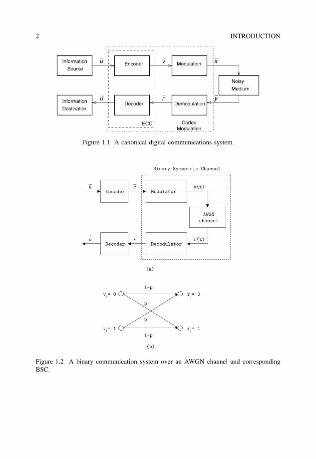
Figure 1.1 shows the block diagram of a canonical digital communications/storagesystem. This is the famous Figure 1 in most books on the theory of ECC and digitalcommunications (Benedetto and Biglieri 1999). The information source and destinationwill include any source coding scheme matched to the nature of the information. The ECCencoder takes as input the information symbols from the source and adds redundant sym-bols to it, so that most of the errors – introduced in the process of modulating a signal,transmitting it over a noisy medium and demodulating it – can be corrected (Massey 1984;McEliece 1977; Moon 2005).
Usually, the channel is assumed to be such that samples of an additive noise processare added to the modulated symbols (in their equivalent complex baseband representation).The noise samples are assumed to be independent from the source symbols. This model isrelatively easy to track mathematically and includes additive white Gaussian noise (AWGN)channels, flat Rayleigh fading channels, and binary symmetric channels (BSC). The case offrequency-selective channels can also be included, as techniques such as spread-spectrumand multicarrier modulation (MCM) effectively transform them into either AWGN channelsor flat Rayleigh fading channels.
At the receiver end, the ECC decoder utilizes the redundant symbols and their rela-tionship with the information symbols in order to correct channel errors. In the case oferror detection, the ECC decoder can be best thought of as a reencoder of the receivedinformation, followed by a check that the redundant symbols generated are the same asthose received.
In classical ECC theory, the combination of modulation, noisy medium and demod-ulation was modeled as a discrete memoryless channel with input v and output r .An example of this is binary transmission over an AWGN channel, which is modeledas a BSC. This is illustrated in Figure 1.2. The BSC has a probability of channelerror p – or transition probability – equal to the probability of a bit error for binary
The Art of Error Correcting Coding, Second Edition Robert H. Morelos-Zaragoza 2006 John Wiley & Sons, Ltd. ISBN: 0-470-01558-6
2 INTRODUCTION
_
_
_
_
_
~
Encoder
Decoder Demodulation
Noisy
Medium
Information
Source
Destination
Information
u v x
yru
Modulation
ModulationCodedECC
Figure 1.1 A canonical digital communications system.
Encoderu
u r
vModulator
AWGN
channel
Decoder Demodulator
^
Binary Symmetric Channel
v(t)
r(t)
(a)
(b)
vi
i
i
i
= 0
v = 1
r = 0
r = 1
p
p
1−p
1−p
Figure 1.2 A binary communication system over an AWGN channel and correspondingBSC.
INTRODUCTION 3
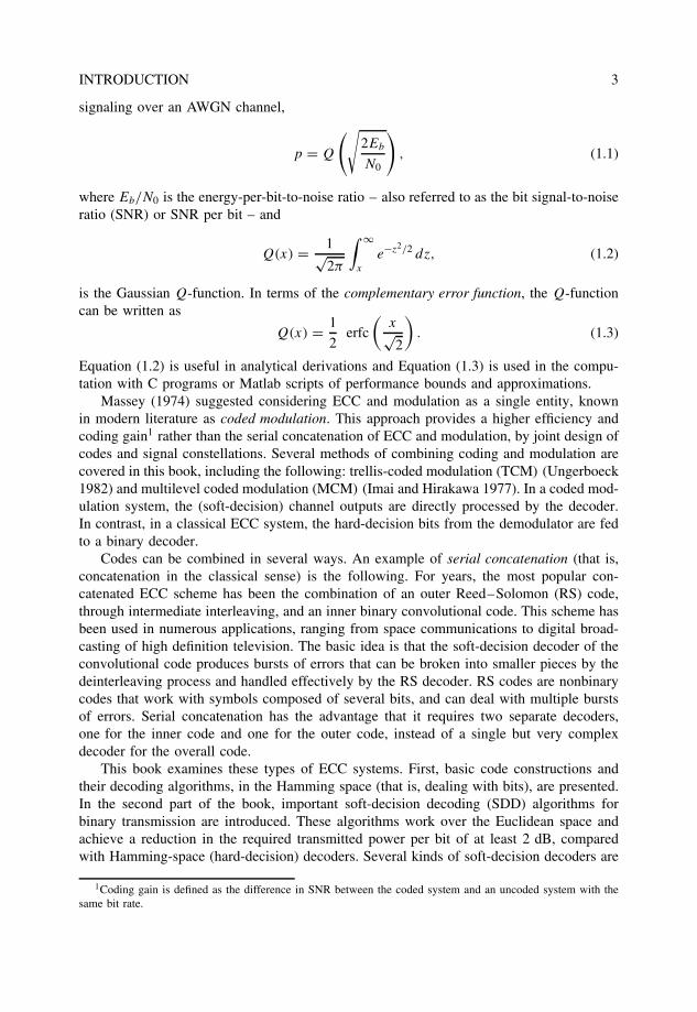
signaling over an AWGN channel,
p = Q
(√2Eb
N0
), (1.1)
where Eb/N0 is the energy-per-bit-to-noise ratio – also referred to as the bit signal-to-noiseratio (SNR) or SNR per bit – and
Q(x) = 1√2π
∫ ∞
x
e−z2/2 dz, (1.2)
is the Gaussian Q-function. In terms of the complementary error function, the Q-functioncan be written as
Q(x) = 1
2erfc
(x√2
). (1.3)
Equation (1.2) is useful in analytical derivations and Equation (1.3) is used in the compu-tation with C programs or Matlab scripts of performance bounds and approximations.
Massey (1974) suggested considering ECC and modulation as a single entity, knownin modern literature as coded modulation. This approach provides a higher efficiency andcoding gain1 rather than the serial concatenation of ECC and modulation, by joint design ofcodes and signal constellations. Several methods of combining coding and modulation arecovered in this book, including the following: trellis-coded modulation (TCM) (Ungerboeck1982) and multilevel coded modulation (MCM) (Imai and Hirakawa 1977). In a coded mod-ulation system, the (soft-decision) channel outputs are directly processed by the decoder.In contrast, in a classical ECC system, the hard-decision bits from the demodulator are fedto a binary decoder.
Codes can be combined in several ways. An example of serial concatenation (that is,concatenation in the classical sense) is the following. For years, the most popular con-catenated ECC scheme has been the combination of an outer Reed–Solomon (RS) code,through intermediate interleaving, and an inner binary convolutional code. This scheme hasbeen used in numerous applications, ranging from space communications to digital broad-casting of high definition television. The basic idea is that the soft-decision decoder of theconvolutional code produces bursts of errors that can be broken into smaller pieces by thedeinterleaving process and handled effectively by the RS decoder. RS codes are nonbinarycodes that work with symbols composed of several bits, and can deal with multiple burstsof errors. Serial concatenation has the advantage that it requires two separate decoders,one for the inner code and one for the outer code, instead of a single but very complexdecoder for the overall code.
This book examines these types of ECC systems. First, basic code constructions andtheir decoding algorithms, in the Hamming space (that is, dealing with bits), are presented.In the second part of the book, important soft-decision decoding (SDD) algorithms forbinary transmission are introduced. These algorithms work over the Euclidean space andachieve a reduction in the required transmitted power per bit of at least 2 dB, comparedwith Hamming-space (hard-decision) decoders. Several kinds of soft-decision decoders are
1Coding gain is defined as the difference in SNR between the coded system and an uncoded system with thesame bit rate.

4 INTRODUCTION
considered, with attention given to their algorithmic aspects (the “how” they work), ratherthan to their theoretical aspects (the ‘why’ they work). Finally, combinations of codes andinterleaving for iterative decoding and of coding and modulation for bandwidth-efficienttransmission are the topic of the last part of the book.
1.1 Error correcting coding: Basic concepts
All error correcting codes are based on the same basic principle: redundancy is added toinformation in order to correct any errors that may occur in the process of transmission orstorage. In a basic (and practical) form, redundant symbols are appended to informationsymbols to obtain a coded sequence or code word. For the purpose of illustration, a codeword obtained by encoding with a block code is shown in Figure 1.3. Such an encodingis said to be systematic. Systematic encoding means that the information symbols alwaysappear in the first (leftmost) k positions of a code word. The remaining (rightmost) n − k
symbols in a code word are a function of the information symbols, and provide redun-dancy that can be used for error correction and/or detection purposes2. The set of all codesequences is called an error correcting code, and will henceforth be denoted by C.
1.1.1 Block codes and convolutional codes
According to the manner in which redundancy is added to messages, ECC can be dividedinto two classes: block and convolutional. Both types of coding schemes have found practi-cal applications. Historically, convolutional codes have been preferred, apparently becauseof the availability of the soft-decision Viterbi decoding algorithm and the belief over manyyears that block codes could not be efficiently decoded with soft-decisions. However, recentdevelopments in the theory and design of SDD algorithms for linear block codes havehelped to dispel this belief. Moreover, the best ECC known to date remain block codes(long irregular low-density parity-check (LDPC) codes).
Block codes process the information on a block-by-block basis, treating each block ofinformation bits independently from others. In other words, block coding is a memorylessoperation, in the sense that code words are independent from each other. In contrast, theoutput of a convolutional encoder depends not only on the current input information, butalso on previous inputs or outputs, either on a block-by-block or a bit-by-bit basis. Forsimplicity of exposition, we begin with a study of the structural properties of block codes.Many of these properties are common to both types of codes.
It should be noted that block codes have, in fact, memory, when encoding is thought ofas a bit-by-bit process and within a code word. Most recently, the difference between block
Information
k symbols
Redundancy
n-k symbols
n symbols
Figure 1.3 A systematic block encoding for error correction.
2Note: Without loss of generality, the order of the information and redundancy can be reversed (i.e., the firstn − k positions in a code word for redundant symbols and the remaining k positions for information symbols).

INTRODUCTION 5
and convolutional codes has become less and less well defined, especially after recentadvances in the understanding of the trellis structure of block codes, and the tail-bitingstructure of some convolutional codes. Indeed, colleagues working on convolutional codessometimes refer to block codes as “codes with time-varying trellis structure.” Similarly,researchers working with block codes may consider convolutional codes as “codes with aregular trellis structure.”
1.1.2 Hamming distance, Hamming spheres and errorcorrecting capability
Consider an error correcting code C with binary elements. As mentioned above, block codesare considered for simplicity of exposition. In order to achieve error correcting capabilities,not all the 2n possible binary vectors of length n are allowed to be transmitted. Instead, C
is a subset of the n-dimensional binary vector space V2 = {0, 1}n, such that its elementsare as far apart as possible.
Consider two vectors x1 = (x1,0, x1,1, . . . , x1,n−1) and x2 = (x2,0, x2,1, . . . , x2,n−1) inV2. Then the Hamming distance between x1 and x2, denoted dH (x1, x2), is defined as thenumber of elements in which the vectors differ,
dH (x1, x2)�= ∣∣ {i : x1,i �= x2,i , 0 ≤ i < n
} ∣∣ =n−1∑i=0
x1,i ⊕ x2,i , (1.4)
where |A| denotes the number of elements in (or the cardinality of) a set A and ⊕ denotesaddition modulo-2 (exclusive-OR).
Given a code C, its minimum Hamming distance, dmin, is defined as the minimumHamming distance among all possible distinct pairs of code words in C,
dmin = minv1,v2∈C
{dH (v1, v2)|v1 �= v2} . (1.5)
Throughout the book, the array (n, k, dmin) is used to denote the parameters of a blockcode of length n, that encodes messages of length k bits and has a minimum Hammingdistance dmin. The assumption is made that the size of the code is |C| = 2k .
Example 1.1.1 The simplest error correcting code is a binary repetition code of length 3.It repeats each bit three times, so that a “0” is encoded onto the vector (000) and a “1”onto the vector (111). Since the two code words differ in all three positions, the Hammingdistance between them is equal to three. Figure 1.4 is a pictorial representation of thiscode. The three-dimensional binary space corresponds to the set of 23 = 8 vertices of thethree-dimensional unit-volume cube. The Hamming distance between code words (000) and(111) equals the number of edges in a path between them. This is equivalent to the numberof coordinates that one needs to change to convert (000) into (111), or vice versa. ThusdH ((000), (111)) = 3. There are only two code words in this case, as a result, dmin = 3.
The binary vector space V2 is also known as a Hamming space. Let v denote a codeword of an error correcting code C. A Hamming sphere St (v), of radius t and centeredaround v, is the set of vectors in V2 at a distance less than or equal to t from the center v,
St (v) = {x ∈ V2|dH (x, v) ≤ t} . (1.6)
6 INTRODUCTION
xx
x
0
1
2
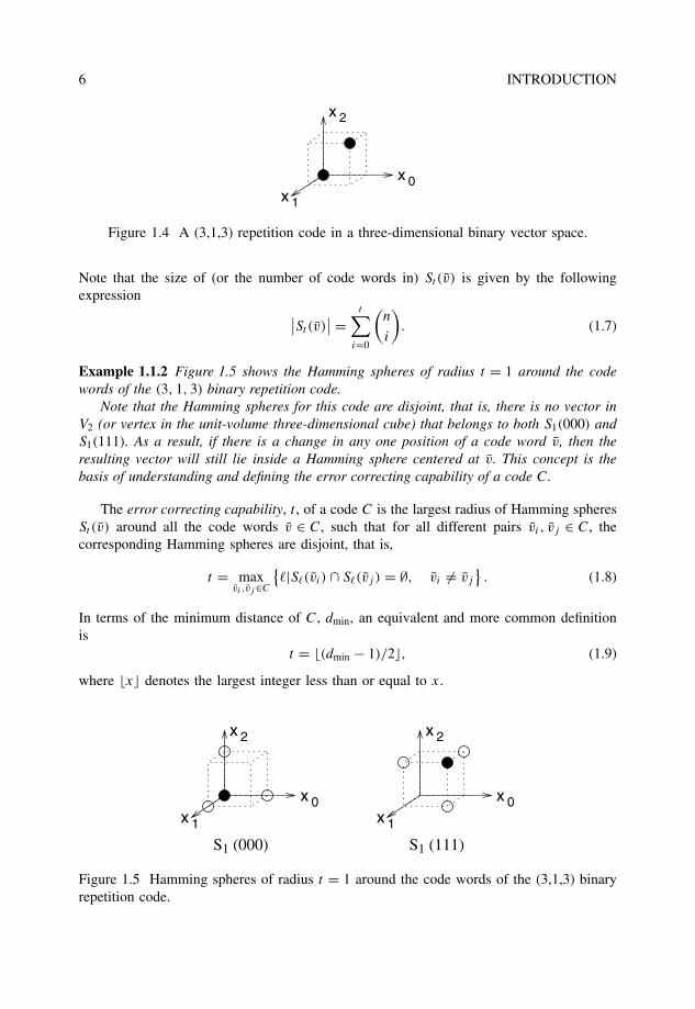
Figure 1.4 A (3,1,3) repetition code in a three-dimensional binary vector space.
Note that the size of (or the number of code words in) St (v) is given by the followingexpression ∣∣St (v)
∣∣ =t∑
i=0
(n
i
). (1.7)
Example 1.1.2 Figure 1.5 shows the Hamming spheres of radius t = 1 around the codewords of the (3, 1, 3) binary repetition code.
Note that the Hamming spheres for this code are disjoint, that is, there is no vector inV2 (or vertex in the unit-volume three-dimensional cube) that belongs to both S1(000) andS1(111). As a result, if there is a change in any one position of a code word v, then theresulting vector will still lie inside a Hamming sphere centered at v. This concept is thebasis of understanding and defining the error correcting capability of a code C.
The error correcting capability, t , of a code C is the largest radius of Hamming spheresSt (v) around all the code words v ∈ C, such that for all different pairs vi , vj ∈ C, thecorresponding Hamming spheres are disjoint, that is,
t = maxvi ,vj∈C
{�|S�(vi) ∩ S�(vj ) = ∅, vi �= vj
}. (1.8)
In terms of the minimum distance of C, dmin, an equivalent and more common definitionis
t = (dmin − 1)/2, (1.9)
where x denotes the largest integer less than or equal to x.
xx
x
0
1
2
xx
x
0
1
2
S1 (111)S1 (000)
Figure 1.5 Hamming spheres of radius t = 1 around the code words of the (3,1,3) binaryrepetition code.
INTRODUCTION 7
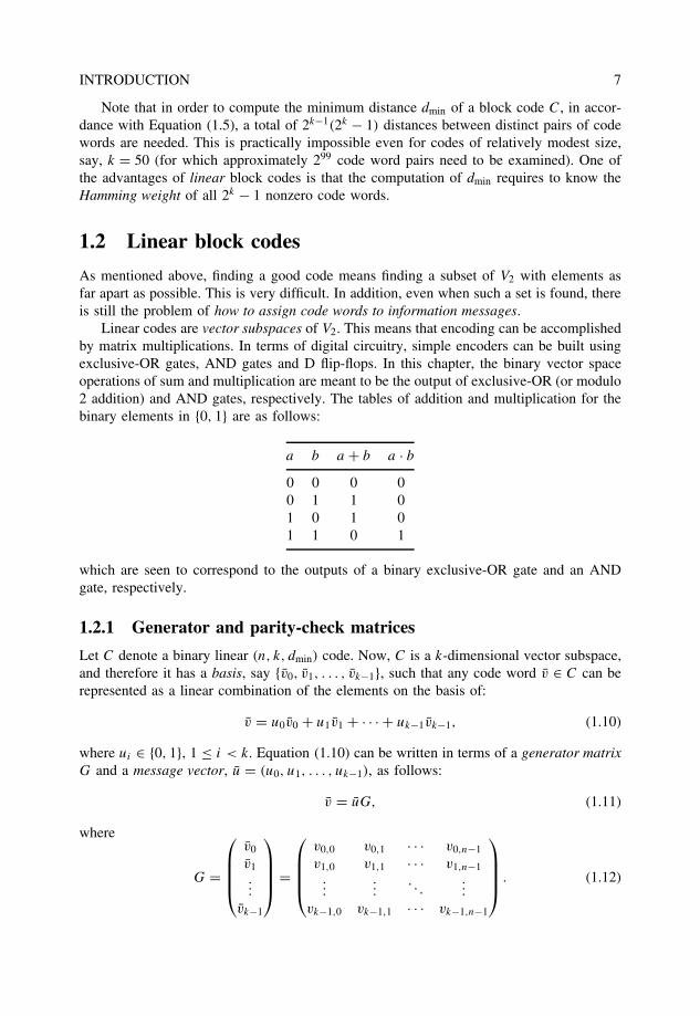
Note that in order to compute the minimum distance dmin of a block code C, in accor-dance with Equation (1.5), a total of 2k−1(2k − 1) distances between distinct pairs of codewords are needed. This is practically impossible even for codes of relatively modest size,say, k = 50 (for which approximately 299 code word pairs need to be examined). One ofthe advantages of linear block codes is that the computation of dmin requires to know theHamming weight of all 2k − 1 nonzero code words.
1.2 Linear block codes
As mentioned above, finding a good code means finding a subset of V2 with elements asfar apart as possible. This is very difficult. In addition, even when such a set is found, thereis still the problem of how to assign code words to information messages.
Linear codes are vector subspaces of V2. This means that encoding can be accomplishedby matrix multiplications. In terms of digital circuitry, simple encoders can be built usingexclusive-OR gates, AND gates and D flip-flops. In this chapter, the binary vector spaceoperations of sum and multiplication are meant to be the output of exclusive-OR (or modulo2 addition) and AND gates, respectively. The tables of addition and multiplication for thebinary elements in {0, 1} are as follows:
a b a + b a · b
0 0 0 00 1 1 01 0 1 01 1 0 1
which are seen to correspond to the outputs of a binary exclusive-OR gate and an ANDgate, respectively.
1.2.1 Generator and parity-check matrices
Let C denote a binary linear (n, k, dmin) code. Now, C is a k-dimensional vector subspace,and therefore it has a basis, say {v0, v1, . . . , vk−1}, such that any code word v ∈ C can berepresented as a linear combination of the elements on the basis of:
v = u0v0 + u1v1 + · · · + uk−1vk−1, (1.10)
where ui ∈ {0, 1}, 1 ≤ i < k. Equation (1.10) can be written in terms of a generator matrixG and a message vector, u = (u0, u1, . . . , uk−1), as follows:
v = uG, (1.11)
where
G =
v0
v1...
vk−1
=
v0,0 v0,1 · · · v0,n−1
v1,0 v1,1 · · · v1,n−1...
.... . .
...
vk−1,0 vk−1,1 · · · vk−1,n−1
. (1.12)
8 INTRODUCTION
Due to the fact that C is a k-dimensional vector space in V2, there is an (n − k)-dimensionaldual space C�, generated by the rows of a matrix H , called the parity-check matrix, suchthat GH� = 0, where H� denotes the transpose of H . In particular, note that for any codeword v ∈ C,
vH� = 0. (1.13)
Equation (1.13) is of fundamental importance in decoding of linear codes, as will be shownin section 1.3.2.
A linear code C⊥ that is generated by H is a binary linear (n, n − k, d⊥min) code, called
the dual code of C.
1.2.2 The weight is the distance
As mentioned in section 1.1.2, a nice feature of linear codes is that computing the minimumdistance of the code amounts to computing the minimum Hamming weight of its nonzerocode words. In this section, this fact is shown. The Hamming weight, wtH (x), of a vectorx = (x0, x1, . . . , xn−1) ∈ V2 is defined as the number of nonzero elements in x, which canbe expressed as the sum
wtH (x) =n−1∑i=0
xi . (1.14)
From the definition of the Hamming distance, it is easy to see that wtH (x) = dH (x, 0). Fora binary linear code C, note that the distance
dH (v1, v2) = dH (v1 + v2, 0) = wtH (v1 + v2) = wtH (v3), (1.15)
where, by linearity, v1 + v2 = v3 ∈ C. As a consequence, the minimum distance of C canbe computed by finding the minimum Hamming weight among the 2k − 1 nonzero codewords. This is simpler than the brute force search among all the pairs of code words,although still a considerable task even for codes of modest size (or dimension k).
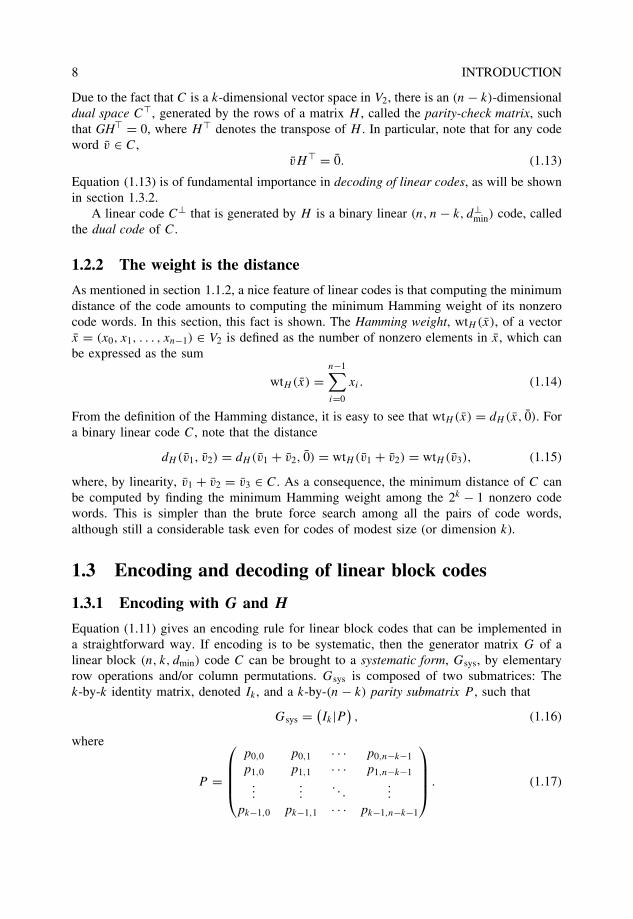
1.3 Encoding and decoding of linear block codes
1.3.1 Encoding with G and H
Equation (1.11) gives an encoding rule for linear block codes that can be implemented ina straightforward way. If encoding is to be systematic, then the generator matrix G of alinear block (n, k, dmin) code C can be brought to a systematic form, Gsys, by elementaryrow operations and/or column permutations. Gsys is composed of two submatrices: Thek-by-k identity matrix, denoted Ik , and a k-by-(n − k) parity submatrix P , such that
Gsys = (Ik|P
), (1.16)
where
P =
p0,0 p0,1 · · · p0,n−k−1
p1,0 p1,1 · · · p1,n−k−1...
.... . .
...
pk−1,0 pk−1,1 · · · pk−1,n−k−1
. (1.17)
INTRODUCTION 9
Since GH� = 0k,n−k, where 0k,n−k denotes the k-by-(n − k) all-zero matrix, it follows thatthe systematic form, Hsys, of the parity-check matrix is
Hsys = (P �|In−k
). (1.18)
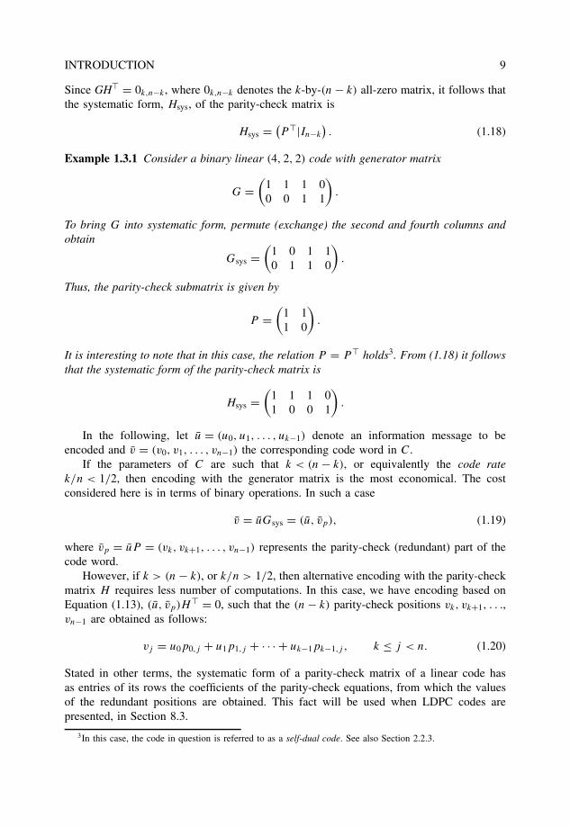
Example 1.3.1 Consider a binary linear (4, 2, 2) code with generator matrix
G =(
1 1 1 00 0 1 1
).
To bring G into systematic form, permute (exchange) the second and fourth columns andobtain
Gsys =(
1 0 1 10 1 1 0
).
Thus, the parity-check submatrix is given by
P =(
1 11 0
).
It is interesting to note that in this case, the relation P = P � holds3. From (1.18) it followsthat the systematic form of the parity-check matrix is
Hsys =(
1 1 1 01 0 0 1
).
In the following, let u = (u0, u1, . . . , uk−1) denote an information message to beencoded and v = (v0, v1, . . . , vn−1) the corresponding code word in C.
If the parameters of C are such that k < (n − k), or equivalently the code ratek/n < 1/2, then encoding with the generator matrix is the most economical. The costconsidered here is in terms of binary operations. In such a case
v = uGsys = (u, vp), (1.19)
where vp = uP = (vk, vk+1, . . . , vn−1) represents the parity-check (redundant) part of thecode word.
However, if k > (n − k), or k/n > 1/2, then alternative encoding with the parity-checkmatrix H requires less number of computations. In this case, we have encoding based onEquation (1.13), (u, vp)H� = 0, such that the (n − k) parity-check positions vk, vk+1, . . .,vn−1 are obtained as follows:
vj = u0p0,j + u1p1,j + · · · + uk−1pk−1,j , k ≤ j < n. (1.20)
Stated in other terms, the systematic form of a parity-check matrix of a linear code hasas entries of its rows the coefficients of the parity-check equations, from which the valuesof the redundant positions are obtained. This fact will be used when LDPC codes arepresented, in Section 8.3.
3In this case, the code in question is referred to as a self-dual code. See also Section 2.2.3.
10 INTRODUCTION
Example 1.3.2 Consider the binary linear (4, 2, 2) code from Example 1.3.1. Let messagesand code words be denoted by u = (u0, u1) and v = (v0, v1, v2, v3), respectively. From(1.20) it follows that
v2 = u0 + u1
v3 = u0
The correspondence between the 22 = 4 two-bit messages and code words is as follows:
(00) → (0000)
(01) → (0110)
(10) → (1011)
(11) → (1101) (1.21)
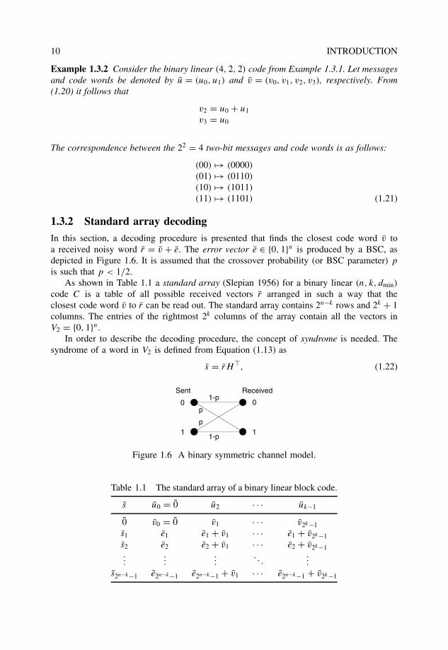
1.3.2 Standard array decoding
In this section, a decoding procedure is presented that finds the closest code word v toa received noisy word r = v + e. The error vector e ∈ {0, 1}n is produced by a BSC, asdepicted in Figure 1.6. It is assumed that the crossover probability (or BSC parameter) p
is such that p < 1/2.As shown in Table 1.1 a standard array (Slepian 1956) for a binary linear (n, k, dmin)
code C is a table of all possible received vectors r arranged in such a way that theclosest code word v to r can be read out. The standard array contains 2n−k rows and 2k + 1columns. The entries of the rightmost 2k columns of the array contain all the vectors inV2 = {0, 1}n.
In order to describe the decoding procedure, the concept of syndrome is needed. Thesyndrome of a word in V2 is defined from Equation (1.13) as
s = rH�, (1.22)
0
1
0
1
Sent Received
1-p
p
p
1-p
Figure 1.6 A binary symmetric channel model.
Table 1.1 The standard array of a binary linear block code.
s u0 = 0 u2 · · · uk−1
0 v0 = 0 v1 · · · v2k−1s1 e1 e1 + v1 · · · e1 + v2k−1s2 e2 e2 + v1 · · · e2 + v2k−1...
......
. . ....
s2n−k−1 e2n−k−1 e2n−k−1 + v1 · · · e2n−k−1 + v2k−1
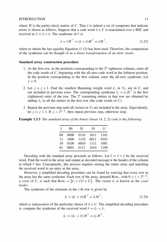
INTRODUCTION 11
where H is the parity-check matrix of C. That s is indeed a set of symptoms that indicateerrors is shown as follows. Suppose that a code word v ∈ C is transmitted over a BSC andreceived as r = v + e. The syndrome of r is
s = rH� = (v + e)H� = eH�, (1.23)
where to obtain the last equality Equation (1.13) has been used. Therefore, the computationof the syndrome can be thought of as a linear transformation of an error vector.
Standard array construction procedure
1. As the first row, in the positions corresponding to the 2k rightmost columns, enter allthe code words of C, beginning with the all-zero code word in the leftmost position.In the position corresponding to the first column, enter the all-zero syndrome. Letj = 0.
2. Let j = j + 1. Find the smallest Hamming weight word ej in V2, not in C, andnot included in previous rows. The corresponding syndrome sj = ejH
� is the first(rightmost) entry of the row. The 2k remaining entries in that row are obtained byadding ej to all the entries in the first row (the code words of C).
3. Repeat the previous step until all vectors in V2 are included in the array. Equivalently,let j = j + 1. If j < 2n−k, then repeat previous step, otherwise stop.
Example 1.3.3 The standard array of the binary linear (4, 2, 2) code is the following:
s 00 01 10 11
00 0000 0110 1011 110111 1000 1110 0011 010110 0100 0010 1111 100101 0001 0111 1010 1100
Decoding with the standard array proceeds as follows. Let r = v + e be the receivedword. Find the word in the array and output as decoded message u the header of the columnin which r lies. Conceptually, this process requires storing the entire array and matchingthe received word to an entry in the array.
However, a simplified decoding procedure can be found by noticing that every row inthe array has the same syndrome. Each row of the array, denoted Rowi , with 0 ≤ i < 2n−k ,a coset of C, is such that Rowi = {
ei + v∣∣v ∈ C
}. The vector ei is known as the coset
leader.The syndrome of the elements in the i-th row is given by
si = (ei + v)H� = eiH�, (1.24)
which is independent of the particular choice of v ∈ C. The simplified decoding procedureis: compute the syndrome of the received word r = ei′ + v,
si′ = (ei′ + v) H� = ei′H�,
12 INTRODUCTION
and find si′ in the leftmost column of the standard array. Then read out the value of ei′ ,from the second column, and add it to the received word to obtain the closest code wordv′ ∈ C to r . Therefore instead of n × 2n bits, standard array decoding can be implementedwith an array of n × 2n−k bits.
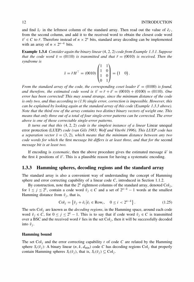
Example 1.3.4 Consider again the binary linear (4, 2, 2) code from Example 1.3.1. Supposethat the code word v = (0110) is transmitted and that r = (0010) is received. Then thesyndrome is
s = rH� = (0010)
1 11 01 00 1
= (
1 0).
From the standard array of the code, the corresponding coset leader e′ = (0100) is found,and therefore, the estimated code word is v′ = r + e′ = (0010) + (0100) = (0110). Oneerror has been corrected! This may sound strange, since the minimum distance of the codeis only two, and thus according to (1.9) single error, correction is impossible. However, thiscan be explained by looking again at the standard array of this code (Example 1.3.3 above).Note that the third row of the array contains two distinct binary vectors of weight one. Thismeans that only three out of a total of four single-error patterns can be corrected. The errorabove is one of those correctable single-error patterns.
It turns out that this (4, 2, 2) code is the simplest instance of a linear Linear unequalerror protection (LUEP) code (van Gils 1983; Wolf and Viterbi 1996). This LUEP code hasa separation vector s = (3, 2), which means that the minimum distance between any twocode words for which the first message bit differs is at least three, and that for the secondmessage bit is at least two.
If encoding is systematic, then the above procedure gives the estimated message u′ inthe first k positions of v′. This is a plausible reason for having a systematic encoding.
1.3.3 Hamming spheres, decoding regions and the standard array
The standard array is also a convenient way of understanding the concept of Hammingsphere and error correcting capability of a linear code C, introduced in Section 1.1.2.
By construction, note that the 2k rightmost columns of the standard array, denoted Colj ,for 1 ≤ j ≤ 2k , contain a code word vj ∈ C and a set of 2n−k − 1 words at the smallestHamming distance from vj , that is,
Colj = {vj + ei
∣∣ei ∈ Rowi , 0 ≤ i < 2n−k}. (1.25)
The sets Colj are known as the decoding regions, in the Hamming space, around each codeword vj ∈ C, for 0 ≤ j ≤ 2k − 1. This is to say that if code word vj ∈ C is transmittedover a BSC and the received word r lies in the set Colj , then it will be successfully decodedinto vj .
Hamming bound
The set Colj and the error correcting capability t of code C are related by the Hammingsphere St (vj ): A binary linear (n, k, dmin) code C has decoding regions Colj that properlycontain Hamming spheres St (vj ), that is, St (vj ) ⊆ Colj .
INTRODUCTION 13
By noticing that the size of Colj is 2n−k, and using Equation (1.7), we obtain thecelebrated Hamming bound
t∑i=0
(n
i
)≤ 2n−k. (1.26)
The Hamming bound has several combinatorial interpretations. One of them is:
The number of syndromes, 2n−k , must be greater than or equal to the numberof correctable error patterns,
∑ti=0
(ni
).
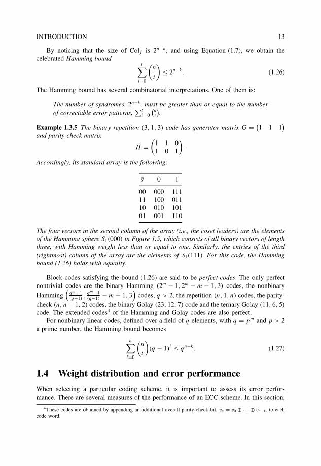
Example 1.3.5 The binary repetition (3, 1, 3) code has generator matrix G = (1 1 1
)and parity-check matrix
H =(
1 1 01 0 1
).
Accordingly, its standard array is the following:
s 0 1
00 000 11111 100 01110 010 10101 001 110
The four vectors in the second column of the array (i.e., the coset leaders) are the elementsof the Hamming sphere S1(000) in Figure 1.5, which consists of all binary vectors of lengththree, with Hamming weight less than or equal to one. Similarly, the entries of the third(rightmost) column of the array are the elements of S1(111). For this code, the Hammingbound (1.26) holds with equality.
Block codes satisfying the bound (1.26) are said to be perfect codes. The only perfectnontrivial codes are the binary Hamming (2m − 1, 2m − m − 1, 3) codes, the nonbinary
Hamming(
qm−1(q−1)
,qm−1(q−1)
− m − 1, 3)
codes, q > 2, the repetition (n, 1, n) codes, the parity-check (n, n − 1, 2) codes, the binary Golay (23, 12, 7) code and the ternary Golay (11, 6, 5)
code. The extended codes4 of the Hamming and Golay codes are also perfect.For nonbinary linear codes, defined over a field of q elements, with q = pm and p > 2
a prime number, the Hamming bound becomes
n∑i=0
(n
i
)(q − 1)i ≤ qn−k. (1.27)
1.4 Weight distribution and error performance
When selecting a particular coding scheme, it is important to assess its error perfor-mance. There are several measures of the performance of an ECC scheme. In this section,
4These codes are obtained by appending an additional overall parity-check bit, vn = v0 ⊕ · · · ⊕ vn−1, to eachcode word.
14 INTRODUCTION
expressions for linear codes are introduced, for three basic channel models: The BSC model,the AWGN channel model and the flat Rayleigh fading channel model.
1.4.1 Weight distribution and undetected error probabilityover a BSC
The weight distribution W(C) of an error correcting code C, is defined as the set of n + 1integers W(C) = {Ai, 0 ≤ i ≤ n}, such that there are Ai code words of Hamming weighti in C, for i = 0, 1, . . . , n.
An expression for the probability of undetected error of a linear code over a BSC isderived next. First, note that the Hamming weight of a word v, wtH (v) equals the Hammingdistance to the all-zero word, wtH (v) = dH (v, 0). Also, as noted before, the Hammingdistance between any two code words v1, v2 in a linear code C equals the Hamming weightof their difference,
dH (v1, v2) = dH (v1 + v2, 0) = wtH (v1 + v2) = wtH (v3),
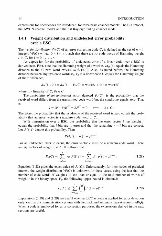
where, by linearity of C, v3 ∈ C.The probability of an undetected error, denoted Pu(C), is the probability that the
received word differs from the transmitted code word but the syndrome equals zero. Thatis,
s = (v + e)H� = eH� = 0 ⇐⇒ e ∈ C.
Therefore, the probability that the syndrome of the received word is zero equals the prob-ability that an error vector is a nonzero code word in C.
With transmission over a BSC, the probability that the error vector e has weight i
equals the probability that i bits are in error and that the remaining n − i bits are correct.Let P (e, i) denote this probability. Then
P (e, i) = pi(1 − p)n−i .
For an undetected error to occur, the error vector e must be a nonzero code word. Thereare Ai vectors of weight i in C. It follows that
Pu(C) =n∑
i=dmin
Ai P (e, i) =n∑
i=dmin
Ai pi(1 − p)n−i . (1.28)
Equation (1.28) gives the exact value of Pu(C). Unfortunately, for most codes of practicalinterest, the weight distribution W(C) is unknown. In these cases, using the fact that thenumber of code words of weight i is less than or equal to the total number of words ofweight i in the binary space V2, the following upper bound is obtained:
Pu(C) ≤n∑
i=dmin
(n
i
)pi(1 − p)n−i . (1.29)
Expressions (1.28) and (1.29) are useful when an ECC scheme is applied for error detectiononly, such as in communication systems with feedback and automatic repeat request (ARQ).When a code is employed for error correction purposes, the expressions derived in the nextsections are useful.
INTRODUCTION 15
1e-10
1e-09
1e-08
1e-07
1e-06
1e-05
0.0001
0.001
0.01
0.1
1
1e-050.00010.0010.010.1
Pu(
C)
p
"Pu(4,2,2)""Pu(4,2,2)_bound"
Figure 1.7 Exact value and upper bound on the probability of undetected error for a binarylinear (4,2,2) code over a BSC.
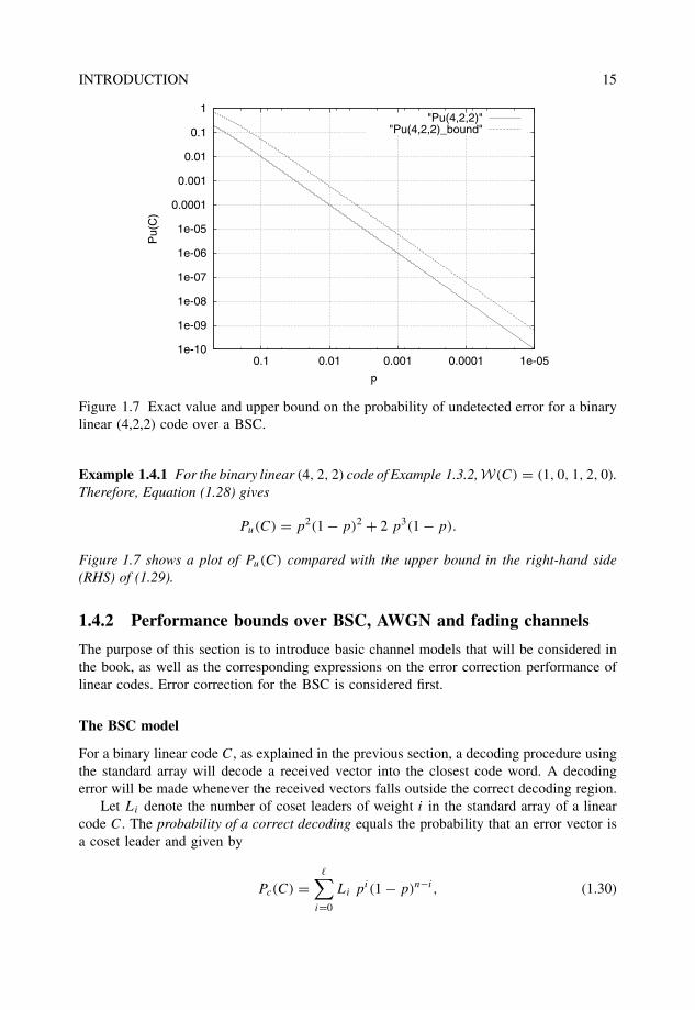
Example 1.4.1 For the binary linear (4, 2, 2) code of Example 1.3.2,W(C) = (1, 0, 1, 2, 0).Therefore, Equation (1.28) gives
Pu(C) = p2(1 − p)2 + 2 p3(1 − p).
Figure 1.7 shows a plot of Pu(C) compared with the upper bound in the right-hand side(RHS) of (1.29).
1.4.2 Performance bounds over BSC, AWGN and fading channels
The purpose of this section is to introduce basic channel models that will be considered inthe book, as well as the corresponding expressions on the error correction performance oflinear codes. Error correction for the BSC is considered first.
The BSC model
For a binary linear code C, as explained in the previous section, a decoding procedure usingthe standard array will decode a received vector into the closest code word. A decodingerror will be made whenever the received vectors falls outside the correct decoding region.
Let Li denote the number of coset leaders of weight i in the standard array of a linearcode C. The probability of a correct decoding equals the probability that an error vector isa coset leader and given by
Pc(C) =�∑
i=0
Li pi(1 − p)n−i , (1.30)
16 INTRODUCTION
where � is the largest Hamming weight of a coset leader e in the standard array. For perfectcodes, � = t , and
Li =(
n
i
), 0 ≤ i ≤ t,
such that, from the Hamming bound (1.26),
�∑i=0
Li =t∑
i=0
(n
i
)= 2n−k.
For binary codes in general, Equation (1.30) becomes a lower bound on Pc(C), sincethere exist coset leaders of weight greater than t .
The probability of incorrect decoding (PID), denoted by Pe(C), also known as theprobability of a decoding error, is equal to the probability of the complement set of theevent of correct decoding, that is, Pe(C) = 1 − Pc(C). From Equation (1.30), it followsthat
Pe(C) = 1 −�∑
i=0
Li pi(1 − p)n−i . (1.31)
Finally, based on the above discussion for Pc(C), the following upper bound is obtained,
Pe(C) ≤ 1 −t∑
i=0
(n
i
)pi(1 − p)n−i , (1.32)
which can also be expressed as
Pe(C) ≤n∑
i=t+1
(n
i
)pi(1 − p)n−i , (1.33)
with equality if, and only if, code C is perfect (satisfies the Hamming bound with equality).
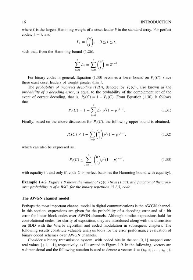
Example 1.4.2 Figure 1.8 shows the values of Pe(C) from (1.33), as a function of the cross-over probability p of a BSC, for the binary repetition (3,1,3) code.
The AWGN channel model
Perhaps the most important channel model in digital communications is the AWGN channel.In this section, expressions are given for the probability of a decoding error and of a biterror for linear block codes over AWGN channels. Although similar expressions hold forconvolutional codes, for clarity of exposition, they are introduced along with the discussionon SDD with the Viterbi algorithm and coded modulation in subsequent chapters. Thefollowing results constitute valuable analysis tools for the error performance evaluation ofbinary coded schemes over AWGN channels.
Consider a binary transmission system, with coded bits in the set {0, 1} mapped ontoreal values {+1, −1}, respectively, as illustrated in Figure 1.9. In the following, vectors aren-dimensional and the following notation is used to denote a vector: x = (x0, x1, . . . , xn−1).
INTRODUCTION 17
1e-10
1e-09
1e-08
1e-07
1e-06
1e-05
0.0001
0.001
0.01
0.1
1
1e-050.00010.0010.010.1
Pe(
C)
p
"Pe(3,1,3)_bound"
Figure 1.8 Probability of a decoding error for the binary repetition (3,1,3) code.
01
+1-1
_ _ _
_
_
Binary encoder
Mappingu v x
+
Soft-decisiondecoder
n
yu~
Informationsource
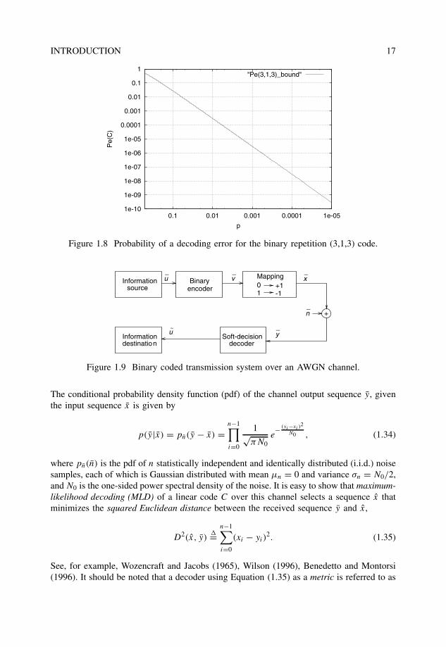
Informationdestination
Figure 1.9 Binary coded transmission system over an AWGN channel.
The conditional probability density function (pdf) of the channel output sequence y, giventhe input sequence x is given by
p(y|x) = pn(y − x) =n−1∏i=0
1√πN0
e− (yi−xi )
2
N0 , (1.34)
where pn(n) is the pdf of n statistically independent and identically distributed (i.i.d.) noisesamples, each of which is Gaussian distributed with mean µn = 0 and variance σn = N0/2,and N0 is the one-sided power spectral density of the noise. It is easy to show that maximum-likelihood decoding (MLD) of a linear code C over this channel selects a sequence x thatminimizes the squared Euclidean distance between the received sequence y and x,
D2(x, y)�=
n−1∑i=0
(xi − yi)2. (1.35)
See, for example, Wozencraft and Jacobs (1965), Wilson (1996), Benedetto and Montorsi(1996). It should be noted that a decoder using Equation (1.35) as a metric is referred to as
18 INTRODUCTION
a soft-decision decoder, independently of whether or not MLD is performed. In Chapter 7,SDD methods are considered.
The probability of a decoding error with MLD, denoted Pe(C), is equal to the probabilitythat a coded sequence x is transmitted and the noise vector n is such that the receivedsequence y = x + n is closer to a different coded sequence x ∈ C, x �= x. For a linear codeC, it can be assumed that the all-zero code word is transmitted. Then Pe(C) can be upperbounded, based on the union bound (Clark and Cain 1981) and the weight distributionW(C), as follows:
Pe(C) ≤n∑
w=dmin
Aw Q
(√2wR
Eb
N0
), (1.36)
where R = k/n is the code rate, Eb/N0 is the energy-per-bit to noise ratio (or SNR perbit) and Q(x) is given by (1.2).
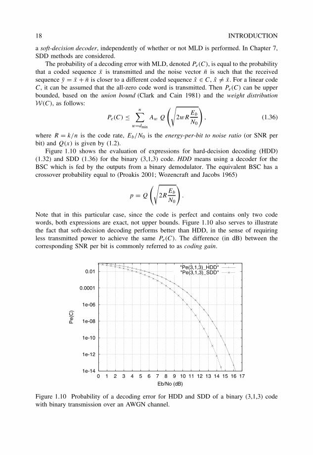
Figure 1.10 shows the evaluation of expressions for hard-decision decoding (HDD)(1.32) and SDD (1.36) for the binary (3,1,3) code. HDD means using a decoder for theBSC which is fed by the outputs from a binary demodulator. The equivalent BSC has acrossover probability equal to (Proakis 2001; Wozencraft and Jacobs 1965)
p = Q
(√2R
Eb
N0
).
Note that in this particular case, since the code is perfect and contains only two codewords, both expressions are exact, not upper bounds. Figure 1.10 also serves to illustratethe fact that soft-decision decoding performs better than HDD, in the sense of requiringless transmitted power to achieve the same Pe(C). The difference (in dB) between thecorresponding SNR per bit is commonly referred to as coding gain.
1e-14
1e-12
1e-10
1e-08
1e-06
0.0001
0.01
0 1 2 3 4 5 6 7 8 9 10 11 12 13 14 15 16 17
Pe(
C)
Eb/No (dB)
"Pe(3,1,3)_HDD""Pe(3,1,3)_SDD"
Figure 1.10 Probability of a decoding error for HDD and SDD of a binary (3,1,3) codewith binary transmission over an AWGN channel.
INTRODUCTION 19
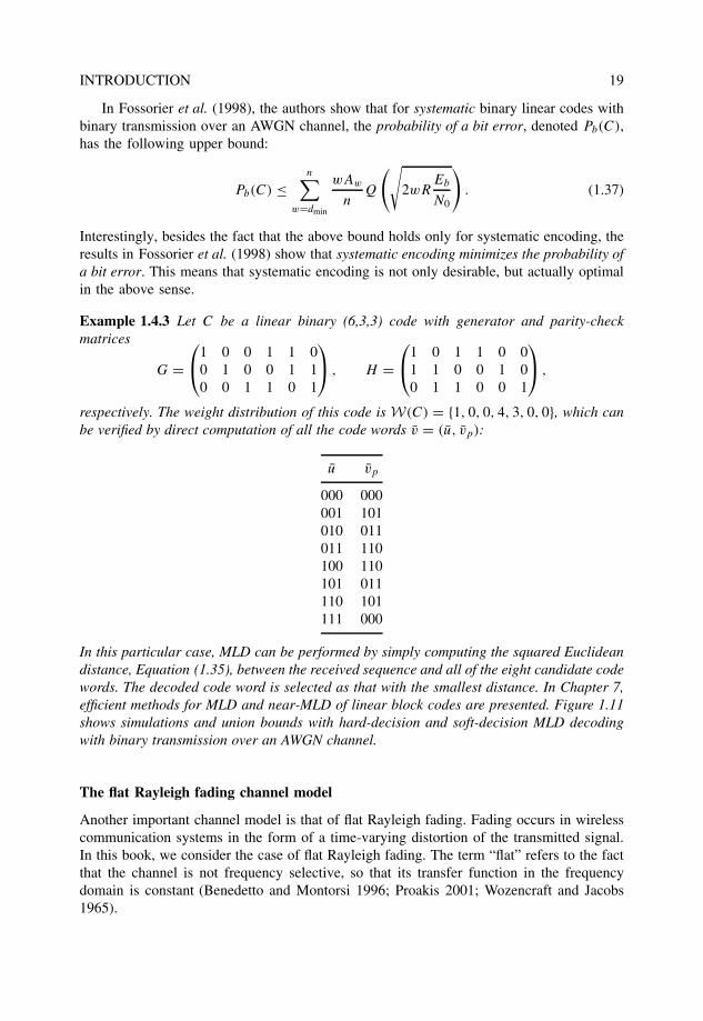
In Fossorier et al. (1998), the authors show that for systematic binary linear codes withbinary transmission over an AWGN channel, the probability of a bit error, denoted Pb(C),has the following upper bound:
Pb(C) ≤n∑
w=dmin
wAw
nQ
(√2wR
Eb
N0
). (1.37)
Interestingly, besides the fact that the above bound holds only for systematic encoding, theresults in Fossorier et al. (1998) show that systematic encoding minimizes the probability ofa bit error. This means that systematic encoding is not only desirable, but actually optimalin the above sense.
Example 1.4.3 Let C be a linear binary (6,3,3) code with generator and parity-checkmatrices
G =1 0 0 1 1 0
0 1 0 0 1 10 0 1 1 0 1
, H =
1 0 1 1 0 0
1 1 0 0 1 00 1 1 0 0 1
,
respectively. The weight distribution of this code is W(C) = {1, 0, 0, 4, 3, 0, 0}, which canbe verified by direct computation of all the code words v = (u, vp):
u vp
000 000001 101010 011011 110100 110101 011110 101111 000
In this particular case, MLD can be performed by simply computing the squared Euclideandistance, Equation (1.35), between the received sequence and all of the eight candidate codewords. The decoded code word is selected as that with the smallest distance. In Chapter 7,efficient methods for MLD and near-MLD of linear block codes are presented. Figure 1.11shows simulations and union bounds with hard-decision and soft-decision MLD decodingwith binary transmission over an AWGN channel.
The flat Rayleigh fading channel model
Another important channel model is that of flat Rayleigh fading. Fading occurs in wirelesscommunication systems in the form of a time-varying distortion of the transmitted signal.In this book, we consider the case of flat Rayleigh fading. The term “flat” refers to the factthat the channel is not frequency selective, so that its transfer function in the frequencydomain is constant (Benedetto and Montorsi 1996; Proakis 2001; Wozencraft and Jacobs1965).
20 INTRODUCTION
1e-05
0.0001
0.001
0.01
0.1
0 1 2 3 4 5 6 7 8 9 10
Pe(
C)
Eb/No (dB)
"Pe(6,3,3)_HDB""Pe(6,3,3)_HDD"
"Pe(6,3,3)_UB""Pe(6,3,3)_SDD"
Figure 1.11 Simulations and union bounds for the binary (6,3,3) code. Binary transmissionover an AWGN channel.
01
+1-1
___
_
_
_
Binary encoder
Mappingu v x
Soft-decisiondecoder
yu~
Informationsource
Informationdestinatio n
n
a
+
x
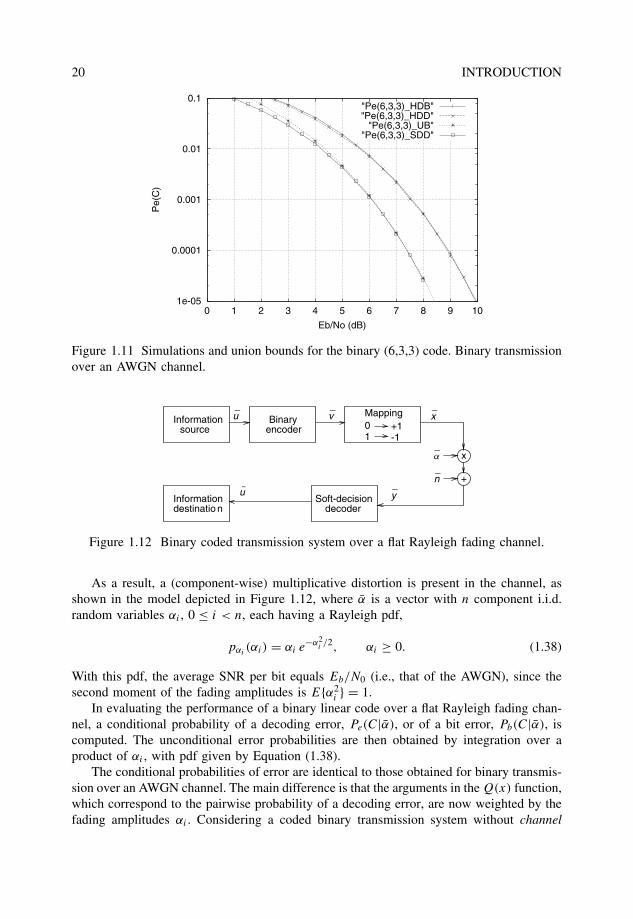
Figure 1.12 Binary coded transmission system over a flat Rayleigh fading channel.
As a result, a (component-wise) multiplicative distortion is present in the channel, asshown in the model depicted in Figure 1.12, where α is a vector with n component i.i.d.random variables αi , 0 ≤ i < n, each having a Rayleigh pdf,
pαi(αi) = αi e−α2
i/2, αi ≥ 0. (1.38)
With this pdf, the average SNR per bit equals Eb/N0 (i.e., that of the AWGN), since thesecond moment of the fading amplitudes is E{α2
i } = 1.In evaluating the performance of a binary linear code over a flat Rayleigh fading chan-
nel, a conditional probability of a decoding error, Pe(C|α), or of a bit error, Pb(C|α), iscomputed. The unconditional error probabilities are then obtained by integration over aproduct of αi , with pdf given by Equation (1.38).
The conditional probabilities of error are identical to those obtained for binary transmis-sion over an AWGN channel. The main difference is that the arguments in the Q(x) function,which correspond to the pairwise probability of a decoding error, are now weighted by thefading amplitudes αi . Considering a coded binary transmission system without channel
INTRODUCTION 21
state information (CSI), we have that
Pe(C|α) ≤n∑
w=dmin
Aw Q
(√1
w�2
w2REb
N0
), (1.39)
with
�w =w∑
i=1
αi. (1.40)
Finally, the probability of a decoding error with binary transmission over a flat Rayleighfading channel is obtained by taking the expectation with respect to �w ,
Pe(C) ≤n∑
w=dmin
Aw
∫ ∞
0Q
(√1
w�2
w2REb
N0
)p�w(�w)d�w. (1.41)
There are several methods to evaluate or further upper bound expression (1.41). One is toevaluate numerically (1.41) by Monte Carlo (MC) integration, with the approximation
Pe(C)<∼ 1
N
N∑�=1
n∑w=dmin
Aw Q
(√2�w(�)R
Eb
N0
), (1.42)
where �w(�) denotes the sum of the squares of w i.i.d. random variables with Rayleighdistribution, given by (1.40), generated in the �-th outcome of a computer program, andN is a sufficiently large number that depends on the range of values of Pe(C). A goodrule of thumb is that N should be at least 100 times larger than the inverse of Pe(C).(See Jeruchim et al. (1992), pp. 500–503.)
Another method is to bound the Q-function by an exponential function (see, e.g.,(Wozencraft and Jacobs 1965), pp. 82–84) and to perform the integration, or to find aChernoff bound. This approach results in a loose bound that, however, yields a closedexpression (see also Wilson (1996), p. 526, and Benedetto and Montorsi (1996), p. 718):
Pe(C) ≤n∑
w=dmin
Aw
1(1 + REb
N0
)w . (1.43)
The bound (1.43) is useful in cases where a first-order estimation of the code performanceis desired.
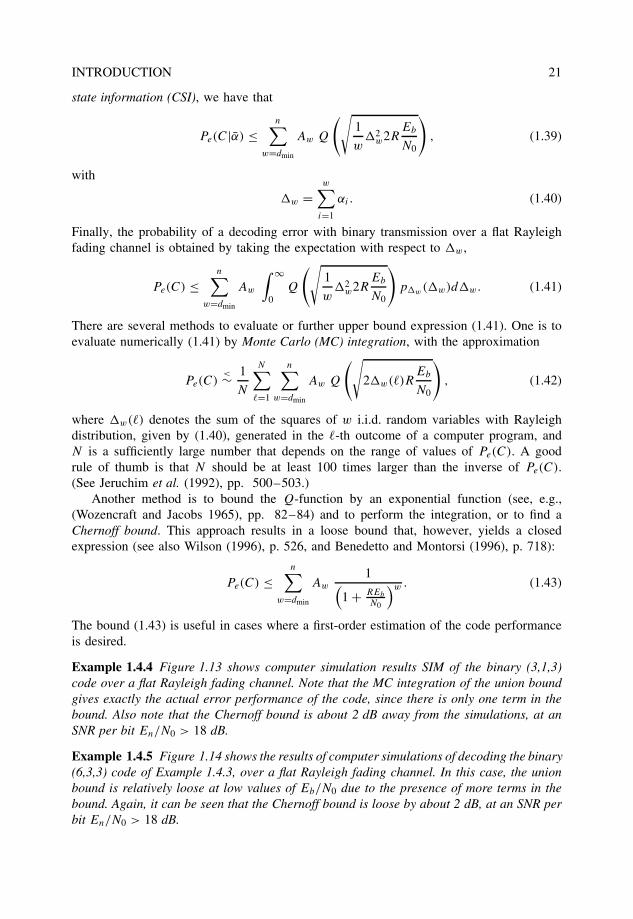
Example 1.4.4 Figure 1.13 shows computer simulation results SIM of the binary (3,1,3)code over a flat Rayleigh fading channel. Note that the MC integration of the union boundgives exactly the actual error performance of the code, since there is only one term in thebound. Also note that the Chernoff bound is about 2 dB away from the simulations, at anSNR per bit En/N0 > 18 dB.
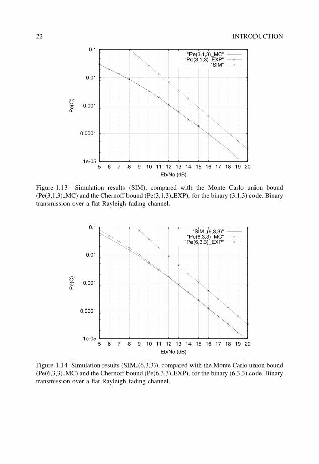
Example 1.4.5 Figure 1.14 shows the results of computer simulations of decoding the binary(6,3,3) code of Example 1.4.3, over a flat Rayleigh fading channel. In this case, the unionbound is relatively loose at low values of Eb/N0 due to the presence of more terms in thebound. Again, it can be seen that the Chernoff bound is loose by about 2 dB, at an SNR perbit En/N0 > 18 dB.
22 INTRODUCTION
1e-05
0.0001
0.001
0.01
0.1
5 6 7 8 9 10 11 12 13 14 15 16 17 18 19 20
Pe(
C)
Eb/No (dB)
"Pe(3,1,3)_MC""Pe(3,1,3)_EXP"
"SIM"
Figure 1.13 Simulation results (SIM), compared with the Monte Carlo union bound(Pe(3,1,3) MC) and the Chernoff bound (Pe(3,1,3) EXP), for the binary (3,1,3) code. Binarytransmission over a flat Rayleigh fading channel.
1e-05
0.0001
0.001
0.01
0.1
5 6 7 8 9 10 11 12 13 14 15 16 17 18 19 20
Pe(
C)
Eb/No (dB)
"SIM_(6,3,3)""Pe(6,3,3)_MC"
"Pe(6,3,3)_EXP"
Figure 1.14 Simulation results (SIM (6,3,3)), compared with the Monte Carlo union bound(Pe(6,3,3) MC) and the Chernoff bound (Pe(6,3,3) EXP), for the binary (6,3,3) code. Binarytransmission over a flat Rayleigh fading channel.
INTRODUCTION 23
Buffer received vector +
_
___Compute
syndromeFind error
vectorr s e
v ’
Figure 1.15 General structure of a hard-decision decoder of a linear block code for theBSC model.
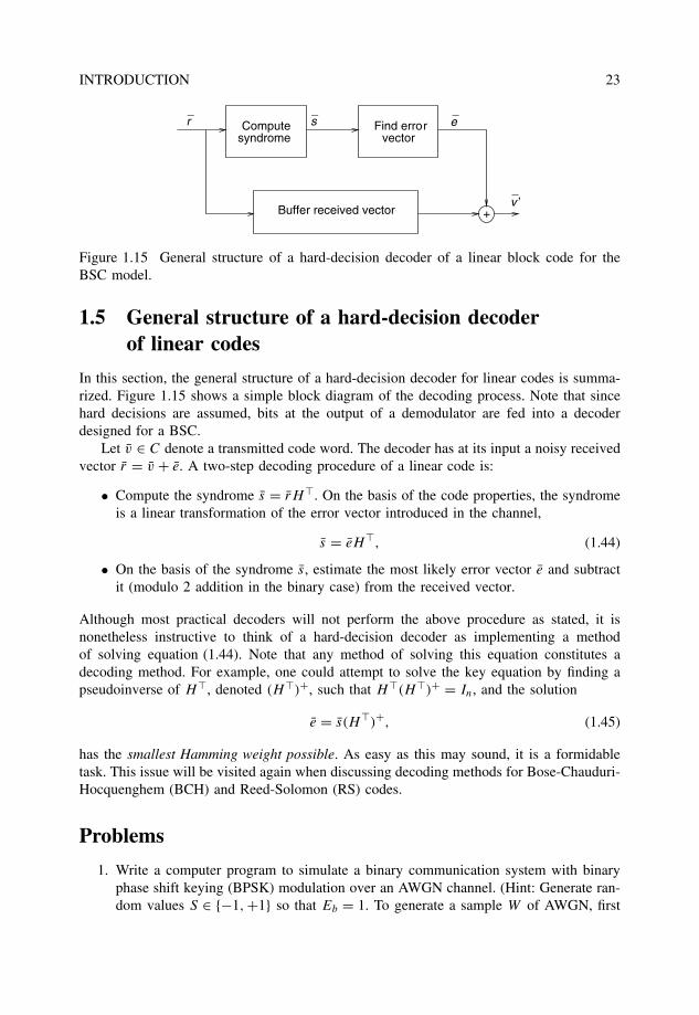
1.5 General structure of a hard-decision decoderof linear codes
In this section, the general structure of a hard-decision decoder for linear codes is summa-rized. Figure 1.15 shows a simple block diagram of the decoding process. Note that sincehard decisions are assumed, bits at the output of a demodulator are fed into a decoderdesigned for a BSC.
Let v ∈ C denote a transmitted code word. The decoder has at its input a noisy receivedvector r = v + e. A two-step decoding procedure of a linear code is:
• Compute the syndrome s = rH�. On the basis of the code properties, the syndromeis a linear transformation of the error vector introduced in the channel,
s = eH�, (1.44)
• On the basis of the syndrome s, estimate the most likely error vector e and subtractit (modulo 2 addition in the binary case) from the received vector.
Although most practical decoders will not perform the above procedure as stated, it isnonetheless instructive to think of a hard-decision decoder as implementing a methodof solving equation (1.44). Note that any method of solving this equation constitutes adecoding method. For example, one could attempt to solve the key equation by finding apseudoinverse of H�, denoted (H�)+, such that H�(H�)+ = In, and the solution
e = s(H�)+, (1.45)
has the smallest Hamming weight possible. As easy as this may sound, it is a formidabletask. This issue will be visited again when discussing decoding methods for Bose-Chauduri-Hocquenghem (BCH) and Reed-Solomon (RS) codes.
Problems
1. Write a computer program to simulate a binary communication system with binaryphase shift keying (BPSK) modulation over an AWGN channel. (Hint: Generate ran-dom values S ∈ {−1, +1} so that Eb = 1. To generate a sample W of AWGN, first
24 INTRODUCTION
generate a Gaussian random variable N of zero mean and unit variance. The transfor-mation W = σW N then results in a Gaussian random variable W of zero mean andvariance σ 2
W = N0/2. Given a value of Eb/N0 in dB, compute N0 =√
10(−(Eb/No)/10).The receiver estimates (RE) the value S based on the sign of the received valueR = S + W . An error event occurs whenever S �= S.)
2. Prove that in general a total of 2k−1(2k − 1) code word pairs need to be examinedin a block code to determine its minimum distance.
3. Prove that GsysHTsys = 0k,n−k.
4. Prove the nonbinary version of the Hamming bound, that is, inequality (1.27).
5. A binary linear block code C has a generator matrix
G =(
1 0 11 1 0
)
(a) Find the weight distribution W(C).
(b) Using elementary matrix operations, bring G into a systematic form G′ thatgenerates a binary linear block code C ′.
(c) Using the weight distribution W(C ′), argue that G and G′ generate the samelinear code, up to a permutation in bit positions.
6. A binary linear block code C has a generator matrix
G =1 0 0 1 1
0 1 0 1 00 0 1 0 1
(a) What are the values of length n and dimension k of this code?
(b) Find the weight distribution W(C) and use it to determine the probability of anundetected error.
(c) Determine the error correcting capability t of C.
(d) Find a parity-check matrix H of C.
(e) Find the standard array of C, based on H of part (c).
(f) Use standard array decoding to find the closest code word to the received wordr = (11011).
7. Carefully sketch circuits used in encoding and decoding of a binary linear (5,3,2)code with generator matrix
G =1 0 0 1 1
0 1 0 1 00 0 1 0 1
INTRODUCTION 25
8. Prove that the decoding region Colj centered around a code word vj ∈ C of a linearcode C contains the Hamming sphere St (vj ), that is,
St (vj ) ⊆ Colj
9. Use the Hamming bound to disprove the existence of a binary linear (32, 24, 5) code.
10. A network designer needs to correct up to 3 random errors in 64 information bits.What is the minimum amount of redundant bits required?
11. A memory system uses a bus with 64 information bits and 16 redundant bits. Withparallel processing (80 bits at a time), what is that maximum number of errors thatcan be corrected?
12. Determine the smallest length of a binary linear code capable of correcting any tworandom bit errors in 21 information bits.
13. Let C be a binary linear (5, 2, dmin) code.
(a) With the aid of the Hamming bound, determine the minimum Hamming distancedmin of C.
(b) Find a generator matrix and a parity-check matrix of C.
(c) Determine the exact probability of a decoding error Pe(C) over a BSC withcrossover probability p.
14. Using the union bound on the error performance of a linear block code with binarytransmission over an AWGN channel, show that the binary (3, 1, 3) repetition codeoffers no advantage over uncoded BPSK modulation. Generalize the result to allbinary (n, 1, n) repetition codes and comment on the basic trade-off involved.
15. Show that the binary (3, 1, 3) repetition code C outperforms BPSK modulation withtransmission over a flat Rayleigh fading channel. Specifically, show that the slope ofthe bit-error-rate (BER) curve of C is three times more negative than that of uncodedbinary phase shift keying (BPSK) modulation. (Thus, C has a diversity order equalto three.)
16. Compare the probability of a bit error, with binary modulation over an AWGN chan-nel, of a binary (3, 1, 3) repetition code and the binary linear (4, 2, 2) code introducedin Example 1.3.1. What is the difference in performance measured in dB?
17. Compare the performance of the two codes in the previous problem with binarytransmission over a Rayleigh fading channel.
18. (Peterson and Weldon (1972)) Given a binary linear (n1, k, d1) code and a binary lin-ear (n2, k, d2) code, construct a binary linear (n1 + n2, k, d) code with d ≥ d1 + d2.
2
Hamming, Golay andReed–Muller codes
In this chapter, important cases of linear binary codes are introduced. They serve to intro-duce more error correcting coding (ECC) concepts, as well as clever decoding algorithms.Hamming codes are perhaps the most widely known class of block codes, with the possi-ble exception of Reed–Solomon codes. As mentioned in Chapter 1, Hamming codes areoptimal in the sense that they require the smallest amount of redundancy, for a givenblock length, to correct any single error. The binary Golay code is the only other nontrivialinstance of an optimal triple-error correcting code. (The only other binary optimal codes arerepetition and single parity-check (SPC) codes.) Reed–Muller (RM) codes can be definedas codes with an elegant combinatorial definition that are easy to decode.
2.1 Hamming codes
From Equation (1.13), any code word v in a linear (n, k, dmin) block code C satisfies
vH� = 0. (2.1)
A useful interpretation of this equation is that the maximum number of linearly independentcolumns of the parity-check matrix H of C is equal to dmin − 1.
In the binary case, for dmin = 3, the above equation translates into the sum of any twocolumns of H not equal to the all-zero vector. Suppose that the columns of H are binaryvectors of length m. There are up to 2m − 1 possible nonzero distinct columns. Therefore,the length of a binary single-error correcting code is given by
n ≤ 2m − 1.
This inequality is precisely the Hamming bound (1.26) for an error correcting code of lengthn, with n − k = m and t = 1. Consequently, a code achieving this bound with equality isknown as a Hamming code.
The Art of Error Correcting Coding, Second Edition Robert H. Morelos-Zaragoza 2006 John Wiley & Sons, Ltd. ISBN: 0-470-01558-6
28 HAMMING, GOLAY AND REED–MULLER CODES
Example 2.1.1 With m = 3, we obtain the Hamming (7, 4, 3) code, with parity-check matrix
H =1 1 1 0 1 0 0
0 1 1 1 0 1 01 1 0 1 0 0 1
.
In the rest of this section, an encoding and decoding algorithm is given that is suitablefor software implementation and for simulation purposes. Later in the book, effective soft-decision decoding algorithms are given, which can be used over real-valued channels suchas the additive white Gaussian noise (AWGN) channel and the Rayleigh fading channel.
As noted before, Hamming codes contain the property of their parity-check matrix H
having different columns, for each and every one. If a single error occurs, in position j ,1 ≤ j ≤ n, then the syndrome of the received vector equals the column of H in the positionin which the error occurred. Let e denote the error vector added in the transmission of acode word over a binary symmetric channel (BSC) channel, and assume that all of itscomponents are equal to zero except for the j -th component, ej = 1. Then, the syndromeof the received word equals
s = rH� = eH� = hj , (2.2)
where hj denotes the j -th column of H , and 1 ≤ j ≤ n.
2.1.1 Encoding and decoding procedures
From Equation (2.2) above, it follows that if it is possible to express the columns of H
as the binary representation of integers, then the value of the syndrome directly gives theposition of the error. This is the idea in the algorithms for encoding and decoding presentedbelow. The columns of the parity-check matrix H are expressed as binary representationsof integer numbers i in the range [1, n] and in increasing order. Let the resulting matrix bedenoted by H ′. Clearly, the code associated with H ′ is equivalent to the original Hammingcode with the parity-check matrix H , up to a permutation (or exchange) of positions.
The parity-check matrix in its systematic form contains the (n − k) × (n − k) identitymatrix, In−k , as in Equation (1.18). Clearly, when expressing H ′ with columns equal to thebinary representation of the (integer) column number, the identity matrix is contained inthose columns of H ′ that correspond to even powers of 2, that is, of the form 2�, 0 ≤ � < m.This is illustrated in the example below.
Example 2.1.2 Let m = 3. Then a systematic parity-check matrix is
H =1 1 0 1 1 0 0
1 0 1 1 0 1 00 1 1 1 0 0 1
,
Matrix H ′ is given by the binary representation of integers 1 to 7 (in the following, thetopmost part corresponds to the least-significant bit (LSB) in the binary representation of aninteger):
H ′ =1 0 1 0 1 0 1
0 1 1 0 0 1 10 0 0 1 1 1 1
,
and matrix In−k is contained in columns 1, 2 and 4.
HAMMING, GOLAY AND REED–MULLER CODES 29
In general, for a (2m − 1, 2m − 1 − m, 3) Hamming code, the identity matrix is con-tained in column numbers 1, 2, 4, . . . , 2m−1 of H ′.
Encoding
Encoding proceeds as dictated by Equation (1.20) of Chapter 1. When computing the paritycheck bit pj , for 1 ≤ j ≤ m, the column position numbers are examined and those which arenot powers of two correspond to message positions; furthermore, the corresponding messagebits are included in the computation. This encoding procedure is somewhat more compli-cated than that of a systematic Hamming code. In return, however, decoding is extremelysimple. Depending on the application, this approach may prove the most appropriate, sinceit is usually decoding that is required to be very fast.
Decoding
Once the code words have been computed in accordance to matrix H ′, the decoding iseasy. The syndrome (2.2) equals the position number in which the error occurred! In adecoding procedure, after the computation of syndrome s, when regarded as an integer, theerroneous position is then corrected as
vs = vs ⊕ 1,
where ⊕ denotes exclusive-or (i.e., 0 ⊕ 0 = 0, 0 ⊕ 1 = 1, 1 ⊕ 0 = 1 and 1 ⊕ 1 = 0).The program hamming.c in the ECC web site implements the above encoding and
decoding procedures for binary Hamming codes.
2.2 The binary Golay code
Golay (Golay 1974) noticed that
3∑i=0
(23
i
)= 211.
This equality shows the possible existence of a perfect binary (23, 12, 7) code, with t = 3,that is, capable of correcting all possible patterns of three errors in 23 bit positions, atthe most. In his paper, Golay gave a generator matrix of such a triple-error correctingbinary code.
Because of its relatively small length (23), dimension (12) and number of redundantbits (11), the binary (23, 12, 7) Golay code can be encoded and decoded simply by usinglook-up tables (LUTs). The program golay23.c in the ECC web site uses a 16 K × 23bits encoding table and an 8 K × 23 bits decoding table.
2.2.1 Encoding
Encoding is based on an LUT that contains a list of all the 212 = 4096 code words, whichare directly indexed by the data. Let u denote a 12-bit binary vector representing the datato be encoded, and let v denote the corresponding 23-bit code word. The encoder LUT is
30 HAMMING, GOLAY AND REED–MULLER CODES
constructed by generating all the 4096 12-bit vectors and by computing the syndrome of apattern for which the 12 most-significant bit (MSB) equal to the information bits and the11 LSB equal to zero. The 11-bit syndrome then becomes the LSB part of the code word.
The LUT is a one-to-one mapping from u onto v, which can be expressed as
v = LUT(u) = (u, get syndrome(u, 0)). (2.3)
In the construction of the encoder LUT, advantage is taken from the cyclic nature ofthe Golay code. Its generator polynomial1 is
g(x) = x11 + x10 + x6 + x5 + x4 + x2 + 1,
which in hexadecimal notation equals C75. This polynomial is used to generate the syn-drome in the procedure “get syndrome” indicated in Equation (2.3) above.
2.2.2 Decoding
Recall from Chapter 1, Figure 1.15, that the decoder’s task is to estimate the most-likely(i.e., least Hamming weight) error vector e from the received vector r . The decoder for theGolay code is based on an LUT that accepts as input the syndrome s of the received vectorr , and outputs the error vector e.The procedure to construct the decoder LUT is as follows:
1. Generate all possible error patterns e of Hamming weight less than or equal to three;
2. For each error pattern, compute the corresponding syndrome s = get syndrome(e);
3. Store at location s of the LUT, the error vector e,
LUT(s) = e.
With the decoder LUT, upon reception of a corrupted received word r , the correction ofup to three bit errors is accomplished by the following:
v = r ⊕ LUT (get syndrome(r)) ,
where v denotes the corrected word.
2.2.3 Arithmetic decoding of the extended (24, 12, 8) Golay code
In this section, a decoding procedure for the extended (24, 12, 8) Golay code, C24, ispresented based on an arithmetic decoding algorithm (Vanstone and van Oorschot 1989;Wicker 1995). The algorithm utilizes the rows and columns of the parity submatrix B in theparity-check matrix H = (
B | I12×12). Note that an extended (24, 12, 8) Golay code, C ′
24,which is equivalent to C24 up to a permutation in the bit positions, can be obtained by addingan overall parity-check bit at the end of each code word in the (23, 12, 7) Golay code.
In hexadecimal notation, the 12 rows of B, denoted rowi , 1 ≤ i ≤ 12, are as follows:
0x7ff, 0xee2, 0xdc5, 0xb8b, 0xf16, 0xe2d,0xc5b, 0x8b7, 0x96e, 0xadc, 0xdb8, 0xb71.
1The definition of a generator polynomial is given in Chapter 3.
HAMMING, GOLAY AND REED–MULLER CODES 31
It is interesting to note that submatrix B of the parity-check matrix of C24 satisfies B = B�.This means that code C24 is a self-dual code. Details of self-dual codes are not covered inthis book. Interested readers are referred to (MacWilliams and Sloane 1977; Wicker 1995).
In program golay24.c, the encoding is performed by recurrence with H , as indicatedin Equation (1.20). As before, let wtH (x) denote the Hamming weight of a vector x.
The decoding steps in arithmetic decoding of the extended (24, 12, 8) Golay code areas follows (Vanstone and van Oorschot 1989; Wicker 1995):
1. Compute the syndrome s = rH�.
2. If wtH (s) ≤ 3, then set e = (s, 0) and go to step 8.
3. If wtH (s + rowi ) ≤ 2, then set e = (s + rowi , xi), where xi is a 12-bit vector withonly the i-th coordinate nonzero.
4. Compute sB.
5. If wtH (sB) ≤ 3, then set e = (0, sB) and go to step 8.
6. If wtH (sB + rowi ) ≤ 2, then set e = (xi , sB + rowi ), with xi defined as above, andgo to step 8.
7. r is corrupted by an uncorrectable error pattern, set error failure flag. End of decoding.
8. Set c = r + e. End of decoding.
2.3 Binary Reed–Muller codes
Binary RM codes constitute a family of error correcting codes that are easy to decode usingmajority-logic (ML) circuits. In addition, codes in this family are known to have relativelysimple and highly structured trellises (Lin et al. 1998). Details about trellises of linear blockcodes can be found in Chapter 7.
An elegant definition of binary RM code is obtained with the use of binary polyno-mials (or Boolean functions). With this definition, RM codes become close relatives ofBose–Chauduri–Hocquenghem (BCH) codes and Reed–Solomon codes, all members ofthe class of polynomial codes.2
2.3.1 Boolean polynomials and RM codes
This section closely follows the development of (MacWilliams and Sloane 1977). Let
f (x1, x2, . . . , xm)
denote a Boolean function on m binary-valued variables x1, x2, . . . , xm. It is well knownthat such a function can be specified by a truth table. The truth table lists the value of f
for all 2m combinations of values of its arguments. All the usual Boolean operations suchas AND (conjunction), OR (disjunction) and NOT (negation) can be defined in a Booleanfunction.
2Polynomial codes are presented in Section 3.4.
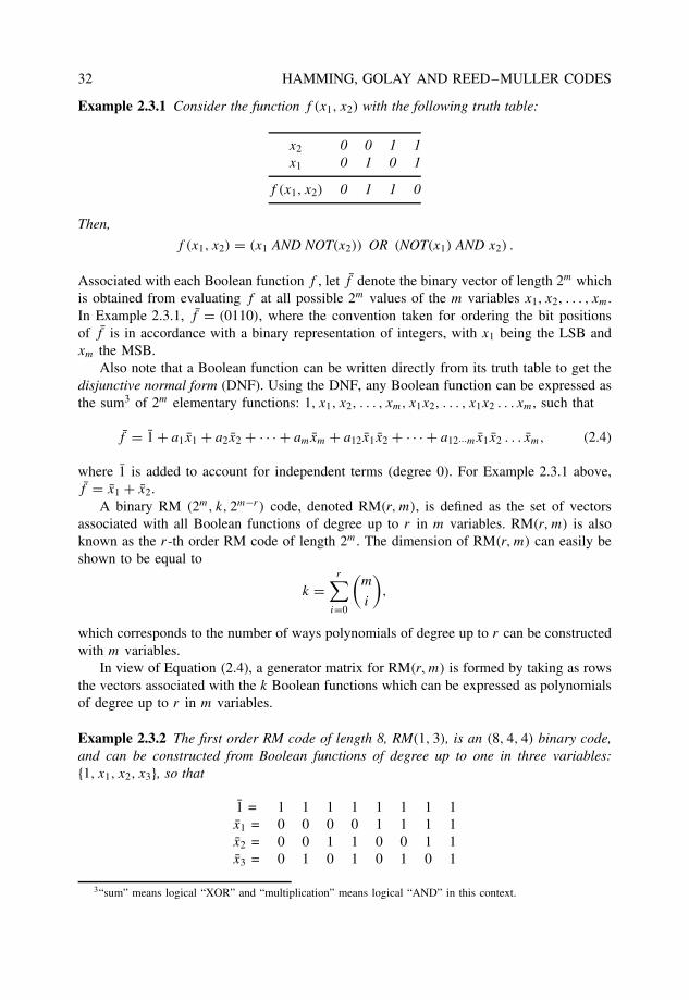
32 HAMMING, GOLAY AND REED–MULLER CODES
Example 2.3.1 Consider the function f (x1, x2) with the following truth table:
x2 0 0 1 1x1 0 1 0 1
f (x1, x2) 0 1 1 0
Then,
f (x1, x2) = (x1 AND NOT(x2)) OR (NOT(x1) AND x2) .
Associated with each Boolean function f , let f denote the binary vector of length 2m whichis obtained from evaluating f at all possible 2m values of the m variables x1, x2, . . . , xm.In Example 2.3.1, f = (0110), where the convention taken for ordering the bit positionsof f is in accordance with a binary representation of integers, with x1 being the LSB andxm the MSB.
Also note that a Boolean function can be written directly from its truth table to get thedisjunctive normal form (DNF). Using the DNF, any Boolean function can be expressed asthe sum3 of 2m elementary functions: 1, x1, x2, . . . , xm, x1x2, . . . , x1x2 . . . xm, such that
f = 1 + a1x1 + a2x2 + · · · + amxm + a12x1x2 + · · · + a12···mx1x2 . . . xm, (2.4)
where 1 is added to account for independent terms (degree 0). For Example 2.3.1 above,f = x1 + x2.
A binary RM (2m, k, 2m−r) code, denoted RM(r, m), is defined as the set of vectorsassociated with all Boolean functions of degree up to r in m variables. RM(r, m) is alsoknown as the r-th order RM code of length 2m. The dimension of RM(r, m) can easily beshown to be equal to
k =r∑
i=0
(m
i
),
which corresponds to the number of ways polynomials of degree up to r can be constructedwith m variables.
In view of Equation (2.4), a generator matrix for RM(r, m) is formed by taking as rowsthe vectors associated with the k Boolean functions which can be expressed as polynomialsof degree up to r in m variables.
Example 2.3.2 The first order RM code of length 8, RM(1, 3), is an (8, 4, 4) binary code,and can be constructed from Boolean functions of degree up to one in three variables:{1, x1, x2, x3}, so that
1 = 1 1 1 1 1 1 1 1x1 = 0 0 0 0 1 1 1 1x2 = 0 0 1 1 0 0 1 1x3 = 0 1 0 1 0 1 0 1
3“sum” means logical “XOR” and “multiplication” means logical “AND” in this context.
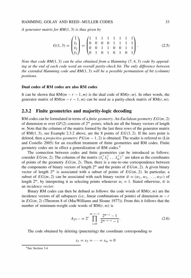
HAMMING, GOLAY AND REED–MULLER CODES 33
A generator matrix for RM(1, 3) is thus given by
G(1, 3) =
1x1
x2
x3
=
1 1 1 1 1 1 1 10 0 0 0 1 1 1 10 0 1 1 0 0 1 10 1 0 1 0 1 0 1
. (2.5)
Note that code RM(1, 3) can be also obtained from a Hamming (7, 4, 3) code by append-ing at the end of each code word an overall parity-check bit. The only difference betweenthe extended Hamming code and RM(1, 3) will be a possible permutation of bit (column)positions.
Dual codes of RM codes are also RM codes
It can be shown that RM(m − r − 1, m) is the dual code of RM(r, m). In other words, thegenerator matrix of RM(m − r − 1, m) can be used as a parity-check matrix of RM(r, m).
2.3.2 Finite geometries and majority-logic decoding
RM codes can be formulated in terms of a finite geometry. An Euclidean geometry EG(m, 2)
of dimension m over GF(2) consists of 2m points, which are all the binary vectors of lengthm. Note that the columns of the matrix formed by the last three rows of the generator matrixof RM(1, 3), see Example 2.3.2 above, are the 8 points of EG(3, 2). If the zero point isdeleted, then a projective geometry PG(m − 1, 2) is obtained. The reader is referred to (Linand Costello 2005) for an excellent treatment of finite geometries and RM codes. Finitegeometry codes are in effect a generalization of RM codes.4
The connection between codes and finite geometries can be introduced as follows:consider EG(m, 2). The columns of the matrix (x�
1 x�2 . . . x�
m)� are taken as the coordinatesof points of the geometry EG(m, 2). Then, there is a one-to-one correspondence betweenthe components of binary vectors of length 2m and the points of EG(m, 2). A given binaryvector of length 2m is associated with a subset of points of EG(m, 2). In particular, asubset of EG(m, 2) can be associated with each binary vector w = (w1, w2, . . . , w2m) oflength 2m, by interpreting it as selecting points whenever wi = 1. Stated otherwise, w isan incidence vector.
Binary RM codes can then be defined as follows: the code words of RM(r, m) are theincidence vectors of all subspaces (i.e., linear combinations of points) of dimension m − r
in EG(m, 2) (Theorem 8 of (MacWilliams and Sloane 1977)). From this it follows that thenumber of minimum-weight code words of RM(r, m) is
A2m−r = 2r
m−r−1∏i=0
2m−i − 1
2m−r−i − 1. (2.6)
The code obtained by deleting (puncturing) the coordinate corresponding to
x1 = x2 = · · · = xm = 0
4See Section 3.4.
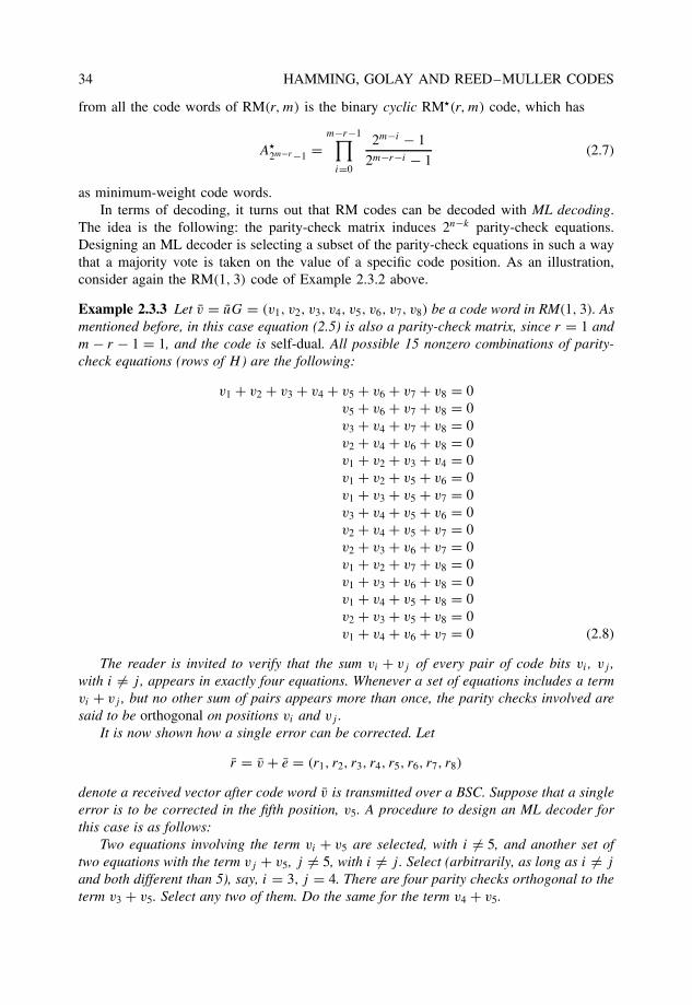
34 HAMMING, GOLAY AND REED–MULLER CODES
from all the code words of RM(r, m) is the binary cyclic RM�(r, m) code, which has
A�2m−r−1 =
m−r−1∏i=0
2m−i − 1
2m−r−i − 1(2.7)
as minimum-weight code words.In terms of decoding, it turns out that RM codes can be decoded with ML decoding.
The idea is the following: the parity-check matrix induces 2n−k parity-check equations.Designing an ML decoder is selecting a subset of the parity-check equations in such a waythat a majority vote is taken on the value of a specific code position. As an illustration,consider again the RM(1, 3) code of Example 2.3.2 above.
Example 2.3.3 Let v = uG = (v1, v2, v3, v4, v5, v6, v7, v8) be a code word in RM(1, 3). Asmentioned before, in this case equation (2.5) is also a parity-check matrix, since r = 1 andm − r − 1 = 1, and the code is self-dual. All possible 15 nonzero combinations of parity-check equations (rows of H ) are the following:
v1 + v2 + v3 + v4 + v5 + v6 + v7 + v8 = 0v5 + v6 + v7 + v8 = 0v3 + v4 + v7 + v8 = 0v2 + v4 + v6 + v8 = 0v1 + v2 + v3 + v4 = 0v1 + v2 + v5 + v6 = 0v1 + v3 + v5 + v7 = 0v3 + v4 + v5 + v6 = 0v2 + v4 + v5 + v7 = 0v2 + v3 + v6 + v7 = 0v1 + v2 + v7 + v8 = 0v1 + v3 + v6 + v8 = 0v1 + v4 + v5 + v8 = 0v2 + v3 + v5 + v8 = 0v1 + v4 + v6 + v7 = 0 (2.8)
The reader is invited to verify that the sum vi + vj of every pair of code bits vi , vj ,with i �= j , appears in exactly four equations. Whenever a set of equations includes a termvi + vj , but no other sum of pairs appears more than once, the parity checks involved aresaid to be orthogonal on positions vi and vj .
It is now shown how a single error can be corrected. Let
r = v + e = (r1, r2, r3, r4, r5, r6, r7, r8)
denote a received vector after code word v is transmitted over a BSC. Suppose that a singleerror is to be corrected in the fifth position, v5. A procedure to design an ML decoder forthis case is as follows:
Two equations involving the term vi + v5 are selected, with i �= 5, and another set oftwo equations with the term vj + v5, j �= 5, with i �= j . Select (arbitrarily, as long as i �= j
and both different than 5), say, i = 3, j = 4. There are four parity checks orthogonal to theterm v3 + v5. Select any two of them. Do the same for the term v4 + v5.
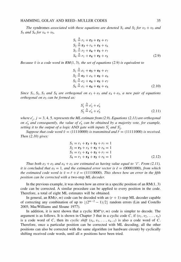
HAMMING, GOLAY AND REED–MULLER CODES 35
The syndromes associated with these equations are denoted S1 and S2 for v3 + v5 andS3 and S4 for v4 + v5,
S1�= r1 + r3 + r5 + r7
S2�= r3 + r4 + r5 + r6
S3�= r2 + r4 + r5 + r7
S4�= r1 + r4 + r5 + r8 (2.9)
Because v is a code word in RM(1, 3), the set of equations (2.9) is equivalent to
S1�= e1 + e3 + e5 + e7
S2�= e3 + e4 + e5 + e6
S3�= e2 + e4 + e5 + e7
S4�= e1 + e4 + e5 + e8 (2.10)
Since S1, S2, S3 and S4 are orthogonal on e3 + e5 and e4 + e5, a new pair of equationsorthogonal on e5 can be formed as:
S ′1
�= e′3 + e′
5
S ′2
�= e′4 + e′
5 (2.11)
where e′j , j = 3, 4, 5, represents the ML estimate from (2.9). Equations (2.11) are orthogonal
on e′5 and consequently, the value of e′
5 can be obtained by a majority vote, for example,setting it to the output of a logic AND gate with inputs S ′
1 and S ′2.
Suppose that code word v = (11110000) is transmitted and r = (11111000) is received.Then (2.10) gives:
S1 = r1 + r3 + r5 + r7 = 1S2 = r3 + r4 + r5 + r6 = 1S3 = r2 + r4 + r5 + r7 = 1S4 = r1 + r4 + r5 + r8 = 1 (2.12)
Thus both e3 + e5 and e4 + e5 are estimated as having value equal to ‘1’. From (2.11),it is concluded that e5 = 1, and the estimated error vector is e = (00001000), from whichthe estimated code word is v = r + e = (11110000). This shows how an error in the fifthposition can be corrected with a two-step ML decoder.
In the previous example, it was shown how an error in a specific position of an RM(1, 3)
code can be corrected. A similar procedure can be applied to every position in the code.Therefore, a total of eight ML estimates will be obtained.
In general, an RM(r, m) code can be decoded with an (r + 1)-step ML decoder capableof correcting any combination of up to �(2m−2 − 1)/2� random errors (Lin and Costello2005; MacWilliams and Sloane 1977).
In addition, it is next shown that a cyclic RM�(r, m) code is simpler to decode. Theargument is as follows. It is shown in Chapter 3 that in a cyclic code C, if (v1, v2, . . . , vn)
is a code word of C, then its cyclic shift (vn, v1, . . . , vn−1) is also a code word of C.Therefore, once a particular position can be corrected with ML decoding, all the otherpositions can also be corrected with the same algorithm (or hardware circuit) by cyclicallyshifting received code words, until all n positions have been tried.
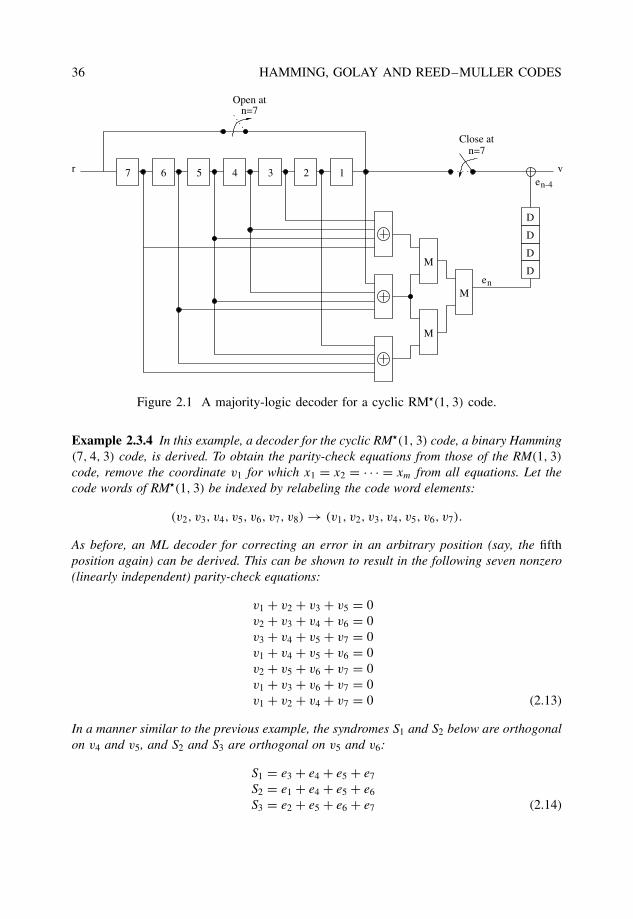
36 HAMMING, GOLAY AND REED–MULLER CODES
D
D
D
D
n=7
67 5 4 3 2 1
M
M
M
re
v
en
n-4
n=7Open at
Close at
Figure 2.1 A majority-logic decoder for a cyclic RM�(1, 3) code.
Example 2.3.4 In this example, a decoder for the cyclic RM�(1, 3) code, a binary Hamming(7, 4, 3) code, is derived. To obtain the parity-check equations from those of the RM(1, 3)
code, remove the coordinate v1 for which x1 = x2 = · · · = xm from all equations. Let thecode words of RM�(1, 3) be indexed by relabeling the code word elements:
(v2, v3, v4, v5, v6, v7, v8) → (v1, v2, v3, v4, v5, v6, v7).
As before, an ML decoder for correcting an error in an arbitrary position (say, the fifthposition again) can be derived. This can be shown to result in the following seven nonzero(linearly independent) parity-check equations:
v1 + v2 + v3 + v5 = 0v2 + v3 + v4 + v6 = 0v3 + v4 + v5 + v7 = 0v1 + v4 + v5 + v6 = 0v2 + v5 + v6 + v7 = 0v1 + v3 + v6 + v7 = 0v1 + v2 + v4 + v7 = 0 (2.13)
In a manner similar to the previous example, the syndromes S1 and S2 below are orthogonalon v4 and v5, and S2 and S3 are orthogonal on v5 and v6:
S1 = e3 + e4 + e5 + e7
S2 = e1 + e4 + e5 + e6
S3 = e2 + e5 + e6 + e7 (2.14)
HAMMING, GOLAY AND REED–MULLER CODES 37
Based on the estimates e′4 + e′
5 and e′5 + e′
6 two additional orthogonal equations on e5 canbe formed to give the final estimate,
S ′1 = e′
4 + e′5
S ′2 = e′
5 + e′6 (2.15)
where e′j , j = 4, 5, 6, represents the ML estimate from the previous step. This results in the
circuit shown in the Figure 2.1. The circuit operates as follows. Initially, the contents of theseven-bit register are set to zero. Suppose that a single error is contained in the received wordin position i, for 1 ≤ i ≤ 7. At each clock cycle, the contents of the register are cyclicallyshifted to the right by one position. Time, in clock cycles, is denoted by the subindex n inthe following.
Consider first the case i = 1. That is, there is an error in the first code word position.After three cycles, the error is contained in register 5 (v5). The output of the ML circuit is setto en = 1. Four cycles later (a total of seven cycles), the first received bit is output and theerror is corrected. Consider now the case i = 7. After nine cycles, the error is detected anden = 1. Again, four cycles later (total 13 cycles), the bit in the last position is output andthe error corrected. This decoder has a latency of 13 cycles. Every 13 cycles, the contentsof the shift register are cleared and a new code word can be processed.
Problems
1. Using the union bound, estimate the probability of a bit error of a binary Hamming(7,4,3) code, denoted CH1, with binary transmission over an AWGN channel.
2. Find the weight distribution of the (23, 12, 7) Golay code.
3. Repeat problem 1 for the binary (23, 12, 7) Golay code, denoted CG. Compare theperformances of CH1 and CG. Comment on the underlying trade-off between thecode rate and the coding gain.
4. Repeat problem 1 with binary transmission over a flat Rayleigh fading channel. (UseMonte Carlo integration for the union bound.)
5. Consider a binary Hamming (15,11) code, denoted CH2.
(a) Give the generator and parity-check matrices in systematic from, denoted Gsys
and Hsys, for this code.
(b) Suppose that the parity-check matrix is rearranged in such a way that the syn-drome vector is the binary representation of an integer denoting the positionof the error. Let Hint denote this matrix. Find the permutation of columns πc
needed to be applied to Hsys in order to obtain Hint.
(c) A code word v = uGsys is sent through a BSC and received with a single erroras r . Show that the syndrome of the vector πc(r) is the binary representationof the position of the error, where πc is the permutation in part (b).
(d) Sketch block diagrams of the circuits used in encoding and decoding CH2.
38 HAMMING, GOLAY AND REED–MULLER CODES
6. Repeat problem 1 for the binary Hamming (15,11,3) code. Compare the performancewith that of the binary Hamming (7,4,3) code. In a binary communication systemover an AWGN channel (no fading) which one of these two codes is expected toperform better?
7. Show that the extended (24,12,8) Golay code is self-dual. (Hint: Show that B = BT .)
8. Prove that the dimension of RM(r, m) is
k =r∑
i=0
(m
i
).
9. Obtain a generator matrix for the Reed–Muller code RM(2, 4).
10. Show that the generator matrix G(r, m) of the r-th order Reed–Muller code RM(r, m)
can be written in terms of the generator matrices of shorter Reed–Muller codes as5
G(r, m) =(
G(r, m − 1) G(r, m − 1)
0 G(r − 1, m − 1)
).
11. Prove that Reed–Muller codes RM(r, m) and RM(m − r − 1, m) are duals.
12. Prove that the Reed–Muller codes satisfy the following subcode property
RM(r1, m) ⊂ RM(r2, m),
where 0 ≤ r1 < r2 ≤ m.
5This is an example of the |u|u + v|-construction, discussed in Section 6.2.
3
Binary cyclic codesand BCH codes
The aim of this chapter is to introduce a minimum set of concepts necessary for theunderstanding of binary cyclic codes and for the efficient implementation of their encodingand decoding procedures. In this chapter, the important family of binary BCH codes isalso introduced. BCH codes are a family of cyclic codes, with an algebraic structure thatis useful in simplifying their encoding and decoding procedures. Binary BCH codes withminimum distance 3, better known as Hamming codes, have been a very popular choice incomputer networks and in memory devices, because of their simple and fast encoding anddecoding. Also, a shortened (48, 36, 5) BCH code was adopted in the U.S. cellular timedivision multiple access (TDMA) system specification, standard IS-54.
3.1 Binary cyclic codes
Cyclic codes are a class of error correcting codes (ECC) that can be efficiently encodedand decoded using simple shift registers and combinatorial logic elements, on the basis oftheir representation using polynomials. In this section, the fundamental concepts of cycliccodes are discussed.
3.1.1 Generator and parity-check polynomials
Let C denote a linear (n, k) block code. Let u and v denote a message and the correspondingcode word in C, respectively. Cyclic codes are linear codes with properties that make themsuitable for hardware implementation. To every code word v a polynomial v(x) is associated,
v = (v0, v1, . . . , vn−1) −→ v(x) = v0 + v1x + · · · vn−1xn−1.
The indeterminant x serves to indicate the relative position of an element vi of v as a termvix
i of v(x), 0 ≤ i < n.
The Art of Error Correcting Coding, Second Edition Robert H. Morelos-Zaragoza 2006 John Wiley & Sons, Ltd. ISBN: 0-470-01558-6
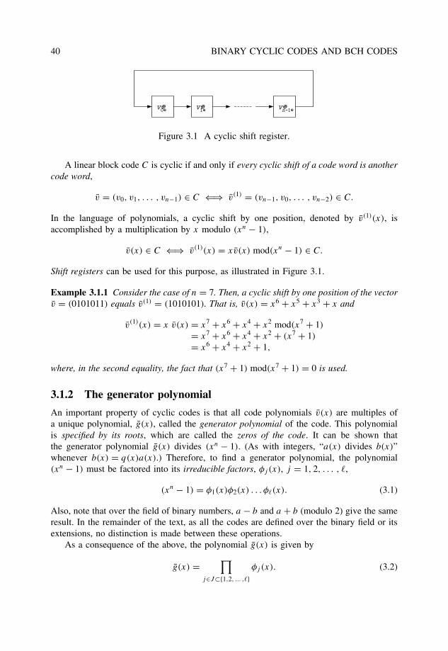
40 BINARY CYCLIC CODES AND BCH CODES
v⊕0⊕ v⊕1⊕ v⊕−n 1⊕
Figure 3.1 A cyclic shift register.
A linear block code C is cyclic if and only if every cyclic shift of a code word is anothercode word,
v = (v0, v1, . . . , vn−1) ∈ C ⇐⇒ v(1) = (vn−1, v0, . . . , vn−2) ∈ C.
In the language of polynomials, a cyclic shift by one position, denoted by v(1)(x), isaccomplished by a multiplication by x modulo (xn − 1),
v(x) ∈ C ⇐⇒ v(1)(x) = xv(x) mod(xn − 1) ∈ C.
Shift registers can be used for this purpose, as illustrated in Figure 3.1.
Example 3.1.1 Consider the case of n = 7. Then, a cyclic shift by one position of the vectorv = (0101011) equals v(1) = (1010101). That is, v(x) = x6 + x5 + x3 + x and
v(1)(x) = x v(x) = x7 + x6 + x4 + x2 mod(x7 + 1)
= x7 + x6 + x4 + x2 + (x7 + 1)
= x6 + x4 + x2 + 1,
where, in the second equality, the fact that (x7 + 1) mod(x7 + 1) = 0 is used.
3.1.2 The generator polynomial
An important property of cyclic codes is that all code polynomials v(x) are multiples ofa unique polynomial, g(x), called the generator polynomial of the code. This polynomialis specified by its roots, which are called the zeros of the code. It can be shown thatthe generator polynomial g(x) divides (xn − 1). (As with integers, “a(x) divides b(x)”whenever b(x) = q(x)a(x).) Therefore, to find a generator polynomial, the polynomial(xn − 1) must be factored into its irreducible factors, φj (x), j = 1, 2, . . . , �,
(xn − 1) = φ1(x)φ2(x) . . . φ�(x). (3.1)
Also, note that over the field of binary numbers, a − b and a + b (modulo 2) give the sameresult. In the remainder of the text, as all the codes are defined over the binary field or itsextensions, no distinction is made between these operations.
As a consequence of the above, the polynomial g(x) is given by
g(x) =∏
j∈J⊂{1,2, ... ,�}φj (x). (3.2)
BINARY CYCLIC CODES AND BCH CODES 41
Example 3.1.2 With coefficients over Z2 = {0, 1}, the polynomial x7 + 1 factors as
x7 + 1 = (x + 1)(x3 + x + 1)(x3 + x2 + 1).
Some examples of cyclic codes of length 7 are:
• A binary cyclic Hamming (7, 4, 3) code is generated by the polynomial
g(x) = x3 + x + 1.
• A binary cyclic parity-check (7, 6, 2) code is generated by
g(x) = (x3 + x + 1)(x3 + x2 + 1).
• A binary maximum-length-sequence (7, 3, 4) code is generated by
g(x) = (x + 1)(x3 + x + 1).
3.1.3 Encoding and decoding of binary cyclic codes
The dimension of a binary cyclic (n, k) code is given by
k = n − deg[g(x)],
where deg[·] denotes the degree of the argument. Since a cyclic code C is also linear, anyset of k linearly independent (LI) vectors can be selected as a generator matrix. In particular,the binary vectors associated with g(x), xg(x), . . . , xk−1g(x) are LI. These vectors canbe used as rows of a generator matrix of C. In this case, a nonsystematic encoding ruleis achieved. That is, the message bits do not appear explicitly in any position of the codewords.
Example 3.1.3 Consider the cyclic Hamming (7, 4, 3) code, with generator polynomial
g(x) = x3 + x + 1 ⇐⇒ g = (1101).
A generator matrix for this code is
G =
1 1 0 1 0 0 00 1 1 0 1 0 00 0 1 1 0 1 00 0 0 1 1 0 1
.
Alternatively, the parity submatrix of a generator matrix of a cyclic code can be con-structed with the vectors associated with the following polynomials:
xn−1 mod g(x),...
xn−k+1 mod g(x),
xn−k mod g(x),
and a systematic encoding is obtained, as illustrated in the example below.
42 BINARY CYCLIC CODES AND BCH CODES
Example 3.1.4 Let C be the cyclic Hamming (7, 4, 3) code. Then g(x) = x3 + x + 1, and
x6 mod(x3 + x + 1) = x2 + 1,
x5 mod(x3 + x + 1) = x2 + x + 1,
x4 mod(x3 + x + 1) = x2 + x,
x3 mod(x3 + x + 1) = x + 1.
It follows that a systematic generator matrix of C is
G =
1 0 0 0 1 0 10 1 0 0 1 1 10 0 1 0 1 1 00 0 0 1 0 1 1
.
Let u(x) be associated with a message to be encoded. Encoding of code words ofa binary cyclic code can be either nonsystematic or systematic, depending on how themessage is processed:
• Nonsystematic encoding
v(x) = u(x) g(x). (3.3)
• Systematic encoding
v(x) = xn−k u(x) + [xn−ku(x) mod g(x)]. (3.4)
3.1.4 The parity-check polynomial
Another polynomial, h(x), called the parity-check polynomial, can be associated withthe parity-check matrix. The generator polynomial and the parity-check polynomial arerelated by
g(x) h(x) = xn + 1. (3.5)
The parity-check polynomial can be computed from the generator polynomial as
h(x) = (xn + 1)/g(x) = h0 + h1x + · · · + hkxk.
Then, a parity-check matrix for C is given by using as rows the binary vectors associatedwith the first n − k − 1 nonzero cyclic shifts
h(j)(x) = xj h(x) mod(xn − 1), j = 0, 1, . . . , n − k − 1.
H =
h0 h1 · · · hk 0 0 · · · 00 h0 h1 · · · · · · hk 0 · · · 00 0 h0 h1 · · · · · · hk · · · 0
0 0 0. . . 0
. . .. . .
. . ....
0 0 0 0 0 · · · · · · · · · hk
. (3.6)
BINARY CYCLIC CODES AND BCH CODES 43
Example 3.1.5 The parity-check polynomial for the cyclic Hamming (7,4,3) code with thegenerator polynomial g(x) = x3 + x + 1 is
h(x) = (x7 + 1)/(x3 + x + 1) = x4 + x2 + x + 1.
A parity-check matrix for this code is
H =1 1 1 0 1 0 0
0 1 1 1 0 1 00 0 1 1 1 0 1
.
In the same manner as with linear codes, systematic encoding can be performed by arecursion with h(x) using
v(x) h(x) = 0 mod(xn + 1).
Systematic encoding can be performed as follows (Lin and Costello 2005; Peterson and Wel-don 1972). Suppose first that the code rate k/n ≤ 0.5. Let u(x) = u0 + u1x + · · · + uk−1
denote a polynomial of degree k − 1, whose coefficients u�, � = 0, 1, . . . , k − 1, are themessage bits to be encoded. Let v(x) denote the code polynomial in C corresponding to theinformation polynomial u(x). In the first step, v� = u�, for � = 0, 1, . . . , k − 1. From thecyclic structure of the code, it follows that the redundant bits can be obtained recursivelyvia the parity-check relations
v� =�−1∑j=0
vjh(�−k),j , � = k, k + 1, . . . , n − 1 (3.7)
where h(�−k),j denotes the j -th entry in the (� − k)-th row of matrix (3.6).In the case of high-rate cyclic (n, k) codes, say k/n > 0.5, encoding by the division
of xn−ku(x) by g(x) is more efficient. Either by recursion with h(x) or by division byg(x), the coefficients of the code polynomials are in the systematic form, so that the firstk coefficients are the message bits, and the remaining n − k coefficients constitute theredundant bits.
Figure 3.2 shows the block diagram of an encoder for a binary cyclic code with generatorpolynomial g(x). Initially, the switch (lower right portion of the figure) is in position 1,and the message bits are both transmitted through the channel and simultaneously fed toa sequential circuit that multiplies by xn−k and divides by g(x). After k cycles, the shiftregister contains the remainder of the division, the switch moves to position 2 and thecontents of the register are sent through the channel.
Duals of cyclic codes and maximum-length-sequence codes
By analogy with linear codes, the dual code of a cyclic code C with generator polynomialg(x) is the cyclic code C⊥ generated by the polynomial h(x). The important class ofmaximum-length-sequence (MLS) cyclic codes (Peterson and Weldon 1972) has as membersthe duals of the cyclic Hamming codes. An MLS cyclic (2m − 1, m, 2m−1) code is generatedby the polynomial g(x) = (xn + 1)/p(x), where p(x) is a primitive polynomial.1
1For a definition of primitive polynomial, see page 49.
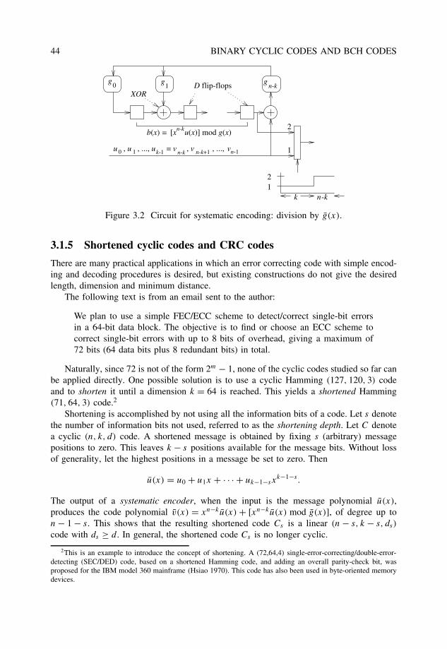
44 BINARY CYCLIC CODES AND BCH CODES
gn-k0
g g1
u , u , ..., u0 1 k-1
n-k[x u(x)] mod g(x)b(x) =
D flip-flopsXOR
n-k n-k+1 n-1 1
2
12
k n-k
= v , v , ..., v
Figure 3.2 Circuit for systematic encoding: division by g(x).
3.1.5 Shortened cyclic codes and CRC codes
There are many practical applications in which an error correcting code with simple encod-ing and decoding procedures is desired, but existing constructions do not give the desiredlength, dimension and minimum distance.
The following text is from an email sent to the author:
We plan to use a simple FEC/ECC scheme to detect/correct single-bit errorsin a 64-bit data block. The objective is to find or choose an ECC scheme tocorrect single-bit errors with up to 8 bits of overhead, giving a maximum of72 bits (64 data bits plus 8 redundant bits) in total.
Naturally, since 72 is not of the form 2m − 1, none of the cyclic codes studied so far canbe applied directly. One possible solution is to use a cyclic Hamming (127, 120, 3) codeand to shorten it until a dimension k = 64 is reached. This yields a shortened Hamming(71, 64, 3) code.2
Shortening is accomplished by not using all the information bits of a code. Let s denotethe number of information bits not used, referred to as the shortening depth. Let C denotea cyclic (n, k, d) code. A shortened message is obtained by fixing s (arbitrary) messagepositions to zero. This leaves k − s positions available for the message bits. Without lossof generality, let the highest positions in a message be set to zero. Then
u(x) = u0 + u1x + · · · + uk−1−sxk−1−s .
The output of a systematic encoder, when the input is the message polynomial u(x),produces the code polynomial v(x) = xn−ku(x) + [xn−ku(x) mod g(x)], of degree up ton − 1 − s. This shows that the resulting shortened code Cs is a linear (n − s, k − s, ds)
code with ds ≥ d. In general, the shortened code Cs is no longer cyclic.
2This is an example to introduce the concept of shortening. A (72,64,4) single-error-correcting/double-error-detecting (SEC/DED) code, based on a shortened Hamming code, and adding an overall parity-check bit, wasproposed for the IBM model 360 mainframe (Hsiao 1970). This code has also been used in byte-oriented memorydevices.
BINARY CYCLIC CODES AND BCH CODES 45
Example 3.1.6 Let C denote the cyclic Hamming (7, 4, 3) code with generator polynomialg(x) = 1 + x + x3. A new code is derived from C by sending 2 leading zeros followed bytwo information bits and the same three redundant bits computed by an encoder in C. Thisprocess gives a set of code words that forms a shortened linear (5, 2, 3) code.
The fundamental property of a shortened code Cs obtained from a cyclic code is that,although the code is generally no longer cyclic, the same encoder and decoder can be used,after the leading zeros are properly taken into account. In computer simulations, it is easyto simply pad the code words with zeros followed by the code word in Cs and use thesame encoding and decoding algorithms discussed in the book. This method is widely usedin hardware implementations of Reed–Solomon decoders. Alternatively, the leading zerosin a message do not need to be included in the code word. Instead, the decoder circuitis modified to multiply the incoming received polynomial r(x) by xn−k+s modulo g(x),instead of xn−k modulo g(x) in the conventional decoder. More details on the modifiedencoder and decoder structures for a shortened cyclic code can be found in Lin and Costello(2005), Peterson and Weldon (1972), Wicker (1995), among other references.
Another possible solution is to try to construct other classes of cyclic codes with thedesired parameters. Good families of cyclic codes not covered in the text are Euclideangeometry (EG) and projective geometry (PG) codes (Lin and Costello 2005).3
Yet another possibility is to use a nonbinary cyclic code, such as the Reed–Solomoncode discussed in Chapter 4, and to express it in terms of bits. This binary image of aReed–Solomon (RS) code will have the additional feature of being able to correct manybursts of errors. Binary images of shortened RS codes have found numerous applications,including memory devices.
CRC codes
One of the most popular forms of ECC are the cyclic redundancy check codes, or CRCcodes. These cyclic codes are used to detect errors in blocks of data. CRC codes are cycliccodes of length n ≤ 2m − 1. Typically, CRC codes have generator polynomials of the form(1 + x)g(x), where g(x) is the generator polynomial of a cyclic Hamming code. Commonvalues of m are 12, 16 and 32. The choice of the generator polynomials is dictated bythe undetected error probability, which depends on the weight distribution of the code.The computation of the undetected error probability of a cyclic code is tantamount todetermining its weight distribution. This has remained an elusive task, even after 50 yearsof coding theory, with some progress reported in Fujiwara et al. (1985), Kazakov (2001)and references therein. Table 3.1 shows a list of the most popular generator polynomials ofCRC codes, or CRC polynomials.
3.1.6 Fire codes
A natural extension of CRC codes are Fire codes. These binary cyclic (n, k, d) codes arecapable of correcting single error bursts of length b or less and have a generator polynomialof the form
g(x) = (x2b−1 + 1)p(x),
3These codes can be used to construct powerful low-density parity-check (LDPC) codes that have excellentperformance with iterative decoding techniques. See Section 8.3 in Chapter 8.
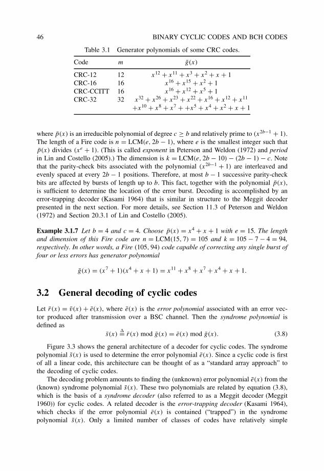
46 BINARY CYCLIC CODES AND BCH CODES
Table 3.1 Generator polynomials of some CRC codes.
Code m g(x)
CRC-12 12 x12 + x11 + x3 + x2 + x + 1CRC-16 16 x16 + x15 + x2 + 1CRC-CCITT 16 x16 + x12 + x5 + 1CRC-32 32 x32 + x26 + x23 + x22 + x16 + x12 + x11
+x10 + x8 + x7 + +x5 + x4 + x2 + x + 1
where p(x) is an irreducible polynomial of degree c ≥ b and relatively prime to (x2b−1 + 1).The length of a Fire code is n = LCM(e, 2b − 1), where e is the smallest integer such thatp(x) divides (xe + 1). (This is called exponent in Peterson and Weldon (1972) and periodin Lin and Costello (2005).) The dimension is k = LCM(e, 2b − 10) − (2b − 1) − c. Notethat the parity-check bits associated with the polynomial (x2b−1 + 1) are interleaved andevenly spaced at every 2b − 1 positions. Therefore, at most b − 1 successive parity-checkbits are affected by bursts of length up to b. This fact, together with the polynomial p(x),is sufficient to determine the location of the error burst. Decoding is accomplished by anerror-trapping decoder (Kasami 1964) that is similar in structure to the Meggit decoderpresented in the next section. For more details, see Section 11.3 of Peterson and Weldon(1972) and Section 20.3.1 of Lin and Costello (2005).
Example 3.1.7 Let b = 4 and c = 4. Choose p(x) = x4 + x + 1 with e = 15. The lengthand dimension of this Fire code are n = LCM(15, 7) = 105 and k = 105 − 7 − 4 = 94,respectively. In other words, a Fire (105, 94) code capable of correcting any single burst offour or less errors has generator polynomial
g(x) = (x7 + 1)(x4 + x + 1) = x11 + x8 + x7 + x4 + x + 1.
3.2 General decoding of cyclic codes
Let r(x) = v(x) + e(x), where e(x) is the error polynomial associated with an error vec-tor produced after transmission over a BSC channel. Then the syndrome polynomial isdefined as
s(x)�= r(x) mod g(x) = e(x) mod g(x). (3.8)
Figure 3.3 shows the general architecture of a decoder for cyclic codes. The syndromepolynomial s(x) is used to determine the error polynomial e(x). Since a cyclic code is firstof all a linear code, this architecture can be thought of as a “standard array approach” tothe decoding of cyclic codes.
The decoding problem amounts to finding the (unknown) error polynomial e(x) from the(known) syndrome polynomial s(x). These two polynomials are related by equation (3.8),which is the basis of a syndrome decoder (also referred to as a Meggit decoder (Meggit1960)) for cyclic codes. A related decoder is the error-trapping decoder (Kasami 1964),which checks if the error polynomial e(x) is contained (“trapped”) in the syndromepolynomial s(x). Only a limited number of classes of codes have relatively simple
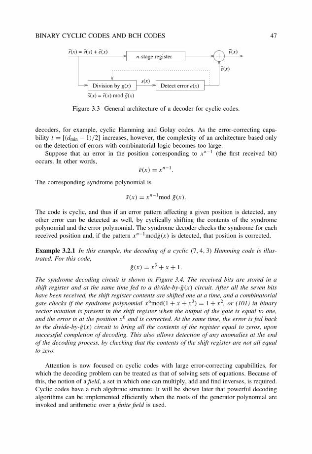
BINARY CYCLIC CODES AND BCH CODES 47
n-stage registerr(x) = v(x) + e(x) v(x)~
s(x)
s(x) = r(x) mod g(x)
e(x)
Division by g(x) Detect error e(x)
Figure 3.3 General architecture of a decoder for cyclic codes.
decoders, for example, cyclic Hamming and Golay codes. As the error-correcting capa-bility t = [(dmin − 1)/2] increases, however, the complexity of an architecture based onlyon the detection of errors with combinatorial logic becomes too large.
Suppose that an error in the position corresponding to xn−1 (the first received bit)occurs. In other words,
e(x) = xn−1.
The corresponding syndrome polynomial is
s(x) = xn−1mod g(x).
The code is cyclic, and thus if an error pattern affecting a given position is detected, anyother error can be detected as well, by cyclically shifting the contents of the syndromepolynomial and the error polynomial. The syndrome decoder checks the syndrome for eachreceived position and, if the pattern xn−1modg(x) is detected, that position is corrected.
Example 3.2.1 In this example, the decoding of a cyclic (7, 4, 3) Hamming code is illus-trated. For this code,
g(x) = x3 + x + 1.
The syndrome decoding circuit is shown in Figure 3.4. The received bits are stored in ashift register and at the same time fed to a divide-by-g(x) circuit. After all the seven bitshave been received, the shift register contents are shifted one at a time, and a combinatorialgate checks if the syndrome polynomial x6mod(1 + x + x3) = 1 + x2, or (101) in binaryvector notation is present in the shift register when the output of the gate is equal to one,and the error is at the position x6 and is corrected. At the same time, the error is fed backto the divide-by-g(x) circuit to bring all the contents of the register equal to zeros, uponsuccessful completion of decoding. This also allows detection of any anomalies at the endof the decoding process, by checking that the contents of the shift register are not all equalto zero.
Attention is now focused on cyclic codes with large error-correcting capabilities, forwhich the decoding problem can be treated as that of solving sets of equations. Because ofthis, the notion of a field, a set in which one can multiply, add and find inverses, is required.Cyclic codes have a rich algebraic structure. It will be shown later that powerful decodingalgorithms can be implemented efficiently when the roots of the generator polynomial areinvoked and arithmetic over a finite field is used.
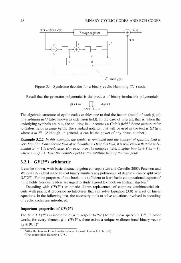
48 BINARY CYCLIC CODES AND BCH CODES
r(x) = v(x) + e(x) v(x)~7-stage register
11 0
x1 x 3
n-1x mod g(x)
e(x)
Figure 3.4 Syndrome decoder for a binary cyclic Hamming (7,4) code.
Recall that the generator polynomial is the product of binary irreducible polynomials:
g(x) =∏
j∈J⊂{1,2,... ,�}φj (x).
The algebraic structure of cyclic codes enables one to find the factors (roots) of each φj (x)
in a splitting field (also known as extension field). In the case of interest, that is, when theunderlying symbols are bits, the splitting field becomes a Galois field.4 Some authors referto Galois fields as finite fields. The standard notation that will be used in the text is GF(q),where q = 2m. (Although, in general, q can be the power of any prime number.)
Example 3.2.2 In this example, the reader is reminded that the concept of splitting field isvery familiar. Consider the field of real numbers. Over this field, it is well known that the poly-nomial x2 + 1 is irreducible. However, over the complex field, it splits into (x + i)(x − i),where i = √−1. Thus the complex field is the splitting field of the real field!
3.2.1 GF(2m) arithmeticIt can be shown, with basic abstract algebra concepts (Lin and Costello 2005; Peterson andWeldon 1972), that in the field of binary numbers any polynomial of degree m can be split overGF(2m). For the purposes of this book, it is sufficient to learn basic computational aspects offinite fields. Serious readers are urged to study a good textbook on abstract algebra.5
Decoding with GF(2m) arithmetic allows replacement of complex combinatorial cir-cuits with practical processor architectures that can solve Equation (3.8) as a set of linearequations. In the following text, the necessary tools to solve equations involved in decodingof cyclic codes are introduced.
Important properties of GF(2m)
The field GF(2m) is isomorphic (with respect to “+”) to the linear space {0, 1}m. In otherwords, for every element β ∈ GF(2m), there exists a unique m-dimensional binary vectorvβ ∈ {0, 1}m.
4After the famous French mathematician Evariste Galois (1811-1832).5The author likes Herstein (1975).
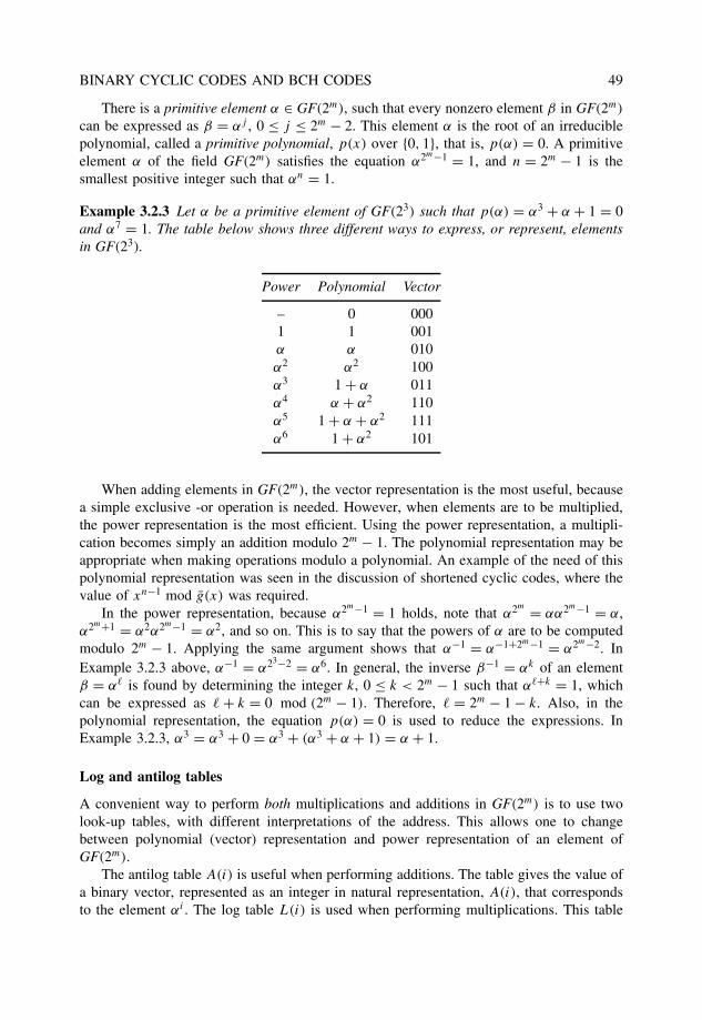
BINARY CYCLIC CODES AND BCH CODES 49
There is a primitive element α ∈ GF(2m), such that every nonzero element β in GF(2m)
can be expressed as β = αj , 0 ≤ j ≤ 2m − 2. This element α is the root of an irreduciblepolynomial, called a primitive polynomial, p(x) over {0, 1}, that is, p(α) = 0. A primitiveelement α of the field GF(2m) satisfies the equation α2m−1 = 1, and n = 2m − 1 is thesmallest positive integer such that αn = 1.
Example 3.2.3 Let α be a primitive element of GF(23) such that p(α) = α3 + α + 1 = 0and α7 = 1. The table below shows three different ways to express, or represent, elementsin GF(23).
Power Polynomial Vector
– 0 0001 1 001α α 010α2 α2 100α3 1 + α 011α4 α + α2 110α5 1 + α + α2 111α6 1 + α2 101
When adding elements in GF(2m), the vector representation is the most useful, becausea simple exclusive -or operation is needed. However, when elements are to be multiplied,the power representation is the most efficient. Using the power representation, a multipli-cation becomes simply an addition modulo 2m − 1. The polynomial representation may beappropriate when making operations modulo a polynomial. An example of the need of thispolynomial representation was seen in the discussion of shortened cyclic codes, where thevalue of xn−1 mod g(x) was required.
In the power representation, because α2m−1 = 1 holds, note that α2m = αα2m−1 = α,α2m+1 = α2α2m−1 = α2, and so on. This is to say that the powers of α are to be computedmodulo 2m − 1. Applying the same argument shows that α−1 = α−1+2m−1 = α2m−2. InExample 3.2.3 above, α−1 = α23−2 = α6. In general, the inverse β−1 = αk of an elementβ = α� is found by determining the integer k, 0 ≤ k < 2m − 1 such that α�+k = 1, whichcan be expressed as � + k = 0 mod (2m − 1). Therefore, � = 2m − 1 − k. Also, in thepolynomial representation, the equation p(α) = 0 is used to reduce the expressions. InExample 3.2.3, α3 = α3 + 0 = α3 + (α3 + α + 1) = α + 1.
Log and antilog tables
A convenient way to perform both multiplications and additions in GF(2m) is to use twolook-up tables, with different interpretations of the address. This allows one to changebetween polynomial (vector) representation and power representation of an element ofGF(2m).
The antilog table A(i) is useful when performing additions. The table gives the value ofa binary vector, represented as an integer in natural representation, A(i), that correspondsto the element αi . The log table L(i) is used when performing multiplications. This table
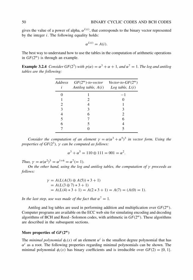
50 BINARY CYCLIC CODES AND BCH CODES
gives the value of a power of alpha, αL(i), that corresponds to the binary vector representedby the integer i. The following equality holds:
αL(i) = A(i).
The best way to understand how to use the tables in the computation of arithmetic operationsin GF(2m) is through an example.
Example 3.2.4 Consider GF(23) with p(α) = α3 + α + 1, and α7 = 1. The log and antilogtables are the following:
Address GF(2m)-to-vector Vector-to-GF(2m)
i Antilog table, A(i) Log table, L(i)
0 1 −11 2 02 4 13 3 34 6 25 7 66 5 47 0 5
Consider the computation of an element γ = α(α3 + α5)3 in vector form. Using theproperties of GF(23), γ can be computed as follows:
α3 + α5 = 110 ⊕ 111 = 001 = α2.
Thus, γ = α(α2)3 = α1+6 = α7(= 1).On the other hand, using the log and antilog tables, the computation of γ proceeds as
follows:
γ = A(L(A(3) ⊕ A(5)) ∗ 3 + 1)
= A(L(3 ⊕ 7) ∗ 3 + 1)
= A(L(4) ∗ 3 + 1) = A(2 ∗ 3 + 1) = A(7) = (A(0) = 1).
In the last step, use was made of the fact that α7 = 1.
Antilog and log tables are used in performing addition and multiplication over GF(2m).Computer programs are available on the ECC web site for simulating encoding and decodingalgorithms of BCH and Reed–Solomon codes, with arithmetic in GF(2m). These algorithmsare described in the subsequent sections.
More properties of GF(2m)
The minimal polynomial φi(x) of an element αi is the smallest degree polynomial that hasαi as a root. The following properties regarding minimal polynomials can be shown. Theminimal polynomial φi(x) has binary coefficients and is irreducible over GF(2) = {0, 1}.

BINARY CYCLIC CODES AND BCH CODES 51
Moreover, φi(x) has roots αi , α2i , . . . , α2κ−1i , where κ divides m. These elements areknown as the conjugate elements of αi in GF(2m). The powers of the conjugate elementsform a cyclotomic coset (see MacWilliams and Sloane (1977), p. 104, and (von zur Gathenand Gerhard 1999), p. 391):
Ci�= {i, 2i, 4i, . . . , 2κ−1i}.
Cyclotomic cosets (also called cycle sets in Peterson and Weldon (1972), p. 209) havethe property that they partition the set I2m−1 of integers modulo 2m − 1. In other words,cyclotomic cosets are disjoint, that is, their intersection is the empty set Ci ∩ Cj = ∅, i �= j ,and the union of all cyclotomic cosets
⋃i Ci = I2m−1.
Example 3.2.5 The cyclotomic sets modulo 7 are:
C0 = {0}C1 = {1, 2, 4}C3 = {3, 6, 5}
The primitive element α of GF(2m) satisfies the equation α2m−1 = 1, and all elements canbe expressed as powers of α. From this it follows that the polynomial (x2m−1 + 1) factorsover the binary field as
(x2m−1 + 1) =M∏
j=0
φ�j(x),
and splits completely over GF(2m) as
(x2m−1 + 1) =2m−2∏j=0
(x + αj ). (3.9)
The order ni of an element β = αi of GF(2m) is the smallest positive integer such thatβni = 1. The order ni of every element in GF(2m) divides 2m − 1.
Importantly, the degree of a minimal polynomial φi(x) is equal to the cardinality (num-ber of elements) of the cyclotomic coset Ci ,
deg [φi(x)] = |Ci |.This suggests the following method for finding all factors of (x2m−1 + 1):
1. Generate the cyclotomic cosets modulo 2m − 1.
2. For each cyclotomic coset Cs , compute the minimal polynomial φs(x) as the productof linear factors (x − αis ), where is ∈ Cs ,
φs(x) =∏is∈Cs
(x + αis ). (3.10)
This method can be used in computing the generator polynomial of any cyclic code of lengthn = 2m − 1. It is used in the computer simulation programs for BCH codes available onthe ECC web site, to compute the generator polynomial given the zeros of the code.
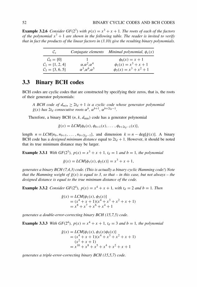
52 BINARY CYCLIC CODES AND BCH CODES
Example 3.2.6 Consider GF(23) with p(x) = x3 + x + 1. The roots of each of the factorsof the polynomial x7 + 1 are shown in the following table. The reader is invited to verifythat in fact the products of the linear factors in (3.10) give the resulting binary polynomials.
Cs Conjugate elements Minimal polynomial, φs(x)
C0 = {0} 1 φ0(x) = x + 1C1 = {1, 2, 4} α,α2,α4 φ1(x) = x3 + x + 1C3 = {3, 6, 5} α3,α6,α5 φ3(x) = x3 + x2 + 1
3.3 Binary BCH codes
BCH codes are cyclic codes that are constructed by specifying their zeros, that is, the rootsof their generator polynomials:
A BCH code of dmin ≥ 2td + 1 is a cyclic code whose generator polynomialg(x) has 2td consecutive roots αb, αb+1, αb+2td−1.
Therefore, a binary BCH (n, k, dmin) code has a generator polynomial
g(x) = LCM{φb(x), φb+1(x), . . . , φb+2td−1(x)},length n = LCM{nb, nb+1, . . . , nb+2td−1}, and dimension k = n − deg[g(x)]. A binaryBCH code has a designed minimum distance equal to 2td + 1. However, it should be notedthat its true minimum distance may be larger.
Example 3.3.1 With GF(23), p(x) = x3 + x + 1, td = 1 and b = 1, the polynomial
g(x) = LCM{φ1(x), φ2(x)} = x3 + x + 1,
generates a binary BCH (7,4,3) code. (This is actually a binary cyclic Hamming code!) Notethat the Hamming weight of g(x) is equal to 3, so that – in this case, but not always – thedesigned distance is equal to the true minimum distance of the code.
Example 3.3.2 Consider GF(24), p(x) = x4 + x + 1, with td = 2 and b = 1. Then
g(x) = LCM{φ1(x), φ3(x)}= (x4 + x + 1)(x4 + x3 + x2 + x + 1)
= x8 + x7 + x6 + x4 + 1
generates a double-error-correcting binary BCH (15,7,5) code.
Example 3.3.3 With GF(24), p(x) = x4 + x + 1, td = 3 and b = 1, the polynomial
g(x) = LCM{φ1(x), φ3(x)φ5(x)}= (x4 + x + 1)(x4 + x3 + x2 + x + 1)
(x2 + x + 1)
= x10 + x8 + x5 + x4 + x2 + x + 1
generates a triple-error-correcting binary BCH (15,5,7) code.
BINARY CYCLIC CODES AND BCH CODES 53
3.3.1 BCH bound
A lower bound on the minimum distance of a BCH code, known as the BCH bound, isderived next. This is useful not only to estimate the error-correcting capabilities of cycliccodes in general, but also to point out particular features of BCH codes. Note that theelements αb, αb+1, . . . , αb+2td−1 are roots of the generator polynomial g(x), and that everycode word v in the BCH code is associated with a polynomial v(x), which is a multiple ofg(x). It follows that
v(x) ∈ C ⇐⇒ v(αi) = 0, b ≤ i < b + 2td . (3.11)
Code word v then satisfies the following set of 2td equations, expressed in matrix form,based on (3.11):
1 1 · · · 1αb αb+1 · · · αb+2td−1
(αb)2 (αb+1)2 · · · (αb+2td−1)2
......
. . ....
(αb)n−1 (αb+1)n−1 . . . (αb+2td−1)n−1
(v0 v1 v2 · · · vn−1
) = 0. (3.12)
Consequently, the parity-check matrix of a binary cyclic BCH code is given by
H =
1 αb (αb)2 · · · (αb)n−1
1 αb+1 (αb+1)2 · · · (αb+1)n−1
......
.... . .
...
1 αb+2td−1 (αb+2td−1)2 · · · (αb+2td−1)n−1
(3.13)
This matrix H has the characteristic that every 2td × 2td submatrix (formed by an arbitraryset of 2td columns of H ) is a Vandermonde matrix (see, e.g., von zur Gathen and Gerhard(1999), p. 95). Therefore (see Section 2.1), any 2td columns of H are linearly independent,from which it follows that the minimum distance of the code is d ≥ 2td + 1. (Petersonand Weldon (1972) p. 270, MacWilliams and Sloane (1977) p. 201, and Lin and Costello(2005) p. 149.) Another interpretation of the results above is the following:
BCH bound If the generator polynomial g(x) of a cyclic (n, k, d) code has � consecutiveroots, say αb, αb+1, . . . , αb+�−1, then d ≥ 2� + 1.
3.4 Polynomial codes
The important class of cyclic polynomial codes includes cyclic RM codes, BCH andReed–Solomon codes, and finite-geometry codes (Kasami et al. 1968; Lin and Costello2005; Peterson and Weldon 1972). Polynomial codes are also specified by setting conditionson their zeros:
Let α be a primitive element of GF(2ms). Let s be a positive integer, and b a divisor of2s − 1. Then αh is a root of the generator polynomial g(x) of a µ-th order polynomial codeif and only if b divides h and
min0≤�<s
W2s (h2�) = jb, with 0 < j <[m
b
]− µ,
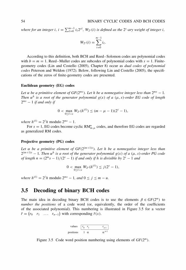
54 BINARY CYCLIC CODES AND BCH CODES
where for an integer i, i = ∑m−1�=0 i�2s�, W2s (i) is defined as the 2s-ary weight of integer i,
W2s (i) =m−1∑i=0
i�.
According to this definition, both BCH and Reed–Solomon codes are polynomial codeswith b = m = 1. Reed–Muller codes are subcodes of polynomial codes with s = 1. Finite-geometry codes (Lin and Costello (2005), Chapter 8) occur as dual codes of polynomialcodes Peterson and Weldon (1972). Below, following Lin and Costello (2005), the specifi-cations of the zeros of finite-geometry codes are presented.
Euclidean geometry (EG) codes
Let α be a primitive element of GF(2ms). Let h be a nonnegative integer less than 2ms − 1.Then αh is a root of the generator polynomial g(x) of a (µ, s)-order EG code of length2ms − 1 if and only if
0 < max0≤�<s
W2s (h(�)) ≤ (m − µ − 1)(2s − 1),
where h(�) = 2�h modulo 2ms − 1.
For s = 1, EG codes become cyclic RM�m,µ codes, and therefore EG codes are regarded
as generalized RM codes.
Projective geometry (PG) codes
Let α be a primitive element of GF(2(m+1)s). Let h be a nonnegative integer less than2(m+1)s − 1. Then αh is a root of the generator polynomial g(x) of a (µ, s)-order PG codeof length n = (2ms − 1)/(2s − 1) if and only if h is divisible by 2s − 1 and
0 < max0≤�<s
W2s (h(�)) ≤ j (2s − 1),
where h(�) = 2�h modulo 2ms − 1, and 0 ≤ j ≤ m − u.
3.5 Decoding of binary BCH codes
The main idea in decoding binary BCH codes is to use the elements β ∈ GF(2m) tonumber the positions of a code word (or, equivalently, the order of the coefficientsof the associated polynomial). This numbering is illustrated in Figure 3.5 for a vectorr = (
r0 r1 . . . rn−1)
with corresponding r(x).
1 α α
r0 r1 rn-1
n-1
values
positions
Figure 3.5 Code word position numbering using elements of GF(2m).
BINARY CYCLIC CODES AND BCH CODES 55
Using GF(2m) arithmetic, the positions of the errors can be found by solving a set ofequations. These equations can be obtained from the error polynomial e(x) and the zerosof the code, αj , for b ≤ j ≤ b + 2td − 1, as shown in the following.
Let r(x) = v(x) + e(x) represent the polynomial associated with a received code word,where the error polynomial is defined as
e(x) = ej1xj1 + ej2x
j2 + · · · + ejν xjν , (3.14)
and ν ≤ td is the number of errors. The sets {ej1, ej2, . . . , ejν }, and {αj1, αj2, . . . , αjν } areknown as the error values and error positions, respectively, where ej ∈ {0, 1} for binaryBCH codes6 and α ∈ GF(2m).
The syndromes are the evaluation of r(x) at each of the zeros of the code:
S1 = r(αb) = ej1αbj1 + · · · + ejνα
bjν
S2 = r(αb+1) = ej1α(b+1)j1 + · · · + ejνα
(b+1)jν
......
S2td = r(αb+2td−1) = ej1α(b+2td−1)j1 + · · · + ejνα
(b+2td−1)jν
and are equivalent to s = Hr�, with H given by (3.13).Let the error-locator polynomial be defined as
σ(x)�=
ν∏�=1
(1 + αj�x) = 1 + σ1x + σ2x2 + · · · + σνx
ν, (3.15)
with roots equal to the inverses of the error locations. Then the following relation betweenthe coefficients of σ(x) and the syndromes holds (see, e.g., Peterson (1974), Lin andCostello (2005) p. 154, Peterson and Weldon (1972) p. 284):
Sν+1
Sν+2...
S2ν
=
S1 S2 · · · Sν
S2 S3 · · · Sν+1...
.... . .
...
Sν Sν+1 · · · S2ν−1
σν
σν−1...
σ1
. (3.16)
Solving the key equation given by (3.16) constitutes the most computationally intensiveoperation in decoding BCH codes. Common methods to solve the key equation are:
1. Berlekamp–Massey algorithm (BMA)
The BMA was invented by Berlekamp (1984), Massey (1969). This is a computation-ally efficient method to solve the key equation, in terms of the number of operationsin GF(2m). The BMA is a popular choice to simulate or implement BCH and RSdecoders in software.
2. Euclidean algorithm (EA)
This is a method to solve the key equation in polynomial form, introduced inSugiyama et al. (1975) and further studied in Mandelbaum (1977). Owing to itsregular structure, the EA is widely used in hardware implementations of BCH andRS decoders.
6It will be seen later that for Reed–Solomon codes ej ∈ GF(2m).
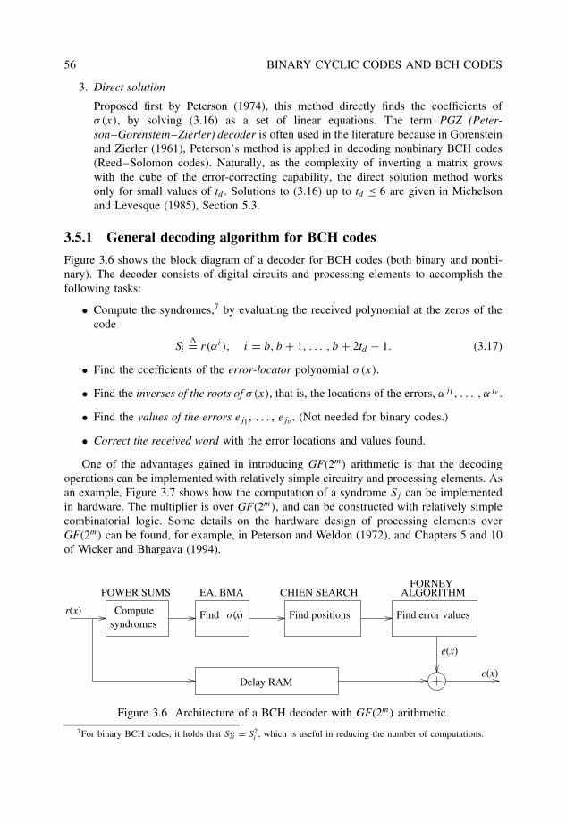
56 BINARY CYCLIC CODES AND BCH CODES
3. Direct solution
Proposed first by Peterson (1974), this method directly finds the coefficients ofσ(x), by solving (3.16) as a set of linear equations. The term PGZ (Peter-son–Gorenstein–Zierler) decoder is often used in the literature because in Gorensteinand Zierler (1961), Peterson’s method is applied in decoding nonbinary BCH codes(Reed–Solomon codes). Naturally, as the complexity of inverting a matrix growswith the cube of the error-correcting capability, the direct solution method worksonly for small values of td . Solutions to (3.16) up to td ≤ 6 are given in Michelsonand Levesque (1985), Section 5.3.
3.5.1 General decoding algorithm for BCH codes
Figure 3.6 shows the block diagram of a decoder for BCH codes (both binary and nonbi-nary). The decoder consists of digital circuits and processing elements to accomplish thefollowing tasks:
• Compute the syndromes,7 by evaluating the received polynomial at the zeros of thecode
Si�= r(αi), i = b, b + 1, . . . , b + 2td − 1. (3.17)
• Find the coefficients of the error-locator polynomial σ(x).
• Find the inverses of the roots of σ(x), that is, the locations of the errors, αj1, . . . , αjν .
• Find the values of the errors ej1 , . . . , ejν . (Not needed for binary codes.)
• Correct the received word with the error locations and values found.
One of the advantages gained in introducing GF(2m) arithmetic is that the decodingoperations can be implemented with relatively simple circuitry and processing elements. Asan example, Figure 3.7 shows how the computation of a syndrome Sj can be implementedin hardware. The multiplier is over GF(2m), and can be constructed with relatively simplecombinatorial logic. Some details on the hardware design of processing elements overGF(2m) can be found, for example, in Peterson and Weldon (1972), and Chapters 5 and 10of Wicker and Bhargava (1994).
Computesyndromes
Find x( )s Find error values
Delay RAM
r(x)
c(x)
e(x)
Find positions
POWER SUMS EA, BMA CHIEN SEARCH ALGORITHMFORNEY
Figure 3.6 Architecture of a BCH decoder with GF(2m) arithmetic.
7For binary BCH codes, it holds that S2i = S2i , which is useful in reducing the number of computations.
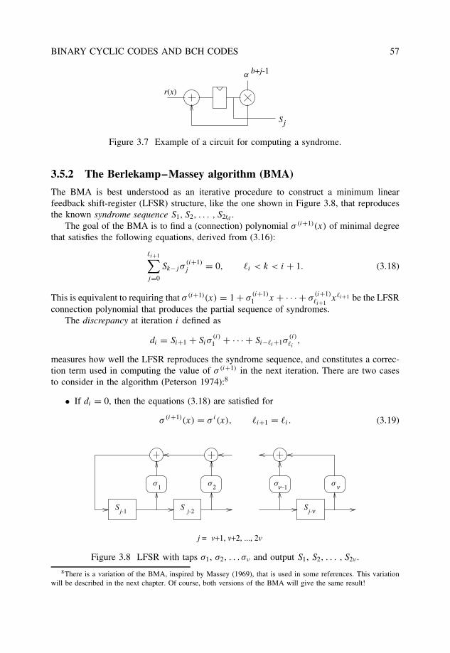
BINARY CYCLIC CODES AND BCH CODES 57
r(x)
Sj
a b+j-1
Figure 3.7 Example of a circuit for computing a syndrome.
3.5.2 The Berlekamp–Massey algorithm (BMA)
The BMA is best understood as an iterative procedure to construct a minimum linearfeedback shift-register (LFSR) structure, like the one shown in Figure 3.8, that reproducesthe known syndrome sequence S1, S2, . . . , S2td .
The goal of the BMA is to find a (connection) polynomial σ (i+1)(x) of minimal degreethat satisfies the following equations, derived from (3.16):
�i+1∑j=0
Sk−j σ(i+1)j = 0, �i < k < i + 1. (3.18)
This is equivalent to requiring that σ (i+1)(x) = 1 + σ(i+1)1 x + · · · + σ
(i+1)�i+1
x�i+1 be the LFSRconnection polynomial that produces the partial sequence of syndromes.
The discrepancy at iteration i defined as
di = Si+1 + Siσ(i)1 + · · · + Si−�i+1σ
(i)�i
,
measures how well the LFSR reproduces the syndrome sequence, and constitutes a correc-tion term used in computing the value of σ (i+1) in the next iteration. There are two casesto consider in the algorithm (Peterson 1974):8
• If di = 0, then the equations (3.18) are satisfied for
σ (i+1)(x) = σ i(x), �i+1 = �i . (3.19)
j = v+1, v+2, ..., 2v
s1
Sj-1
s2
S
s
S
−1ν νs
j-2 j-ν
Figure 3.8 LFSR with taps σ1, σ2, . . . σν and output S1, S2, . . . , S2ν .
8There is a variation of the BMA, inspired by Massey (1969), that is used in some references. This variationwill be described in the next chapter. Of course, both versions of the BMA will give the same result!
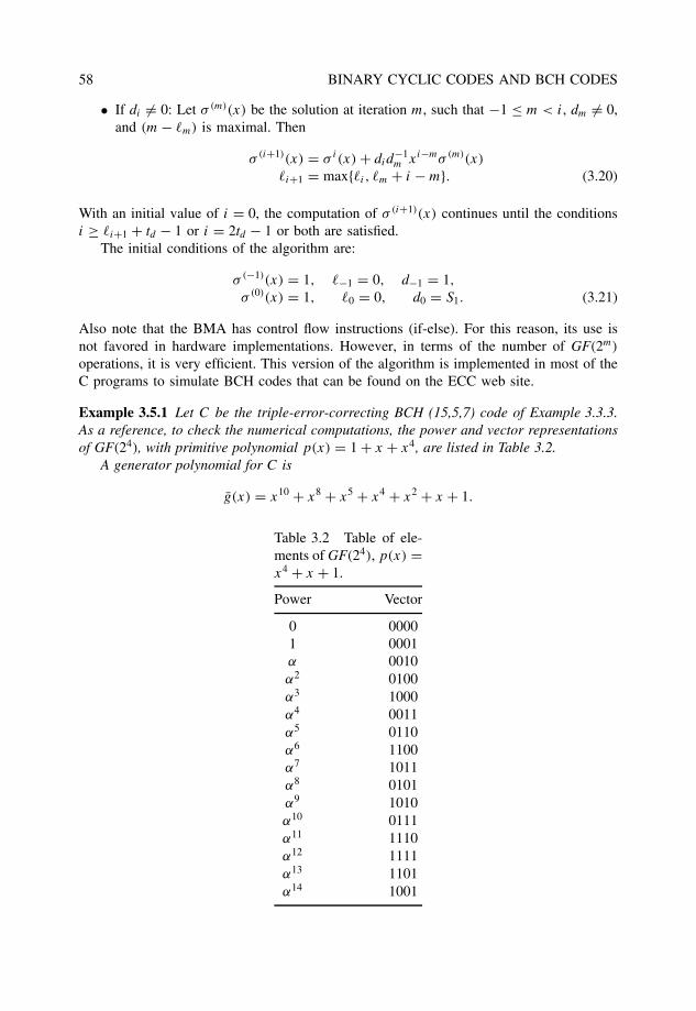
58 BINARY CYCLIC CODES AND BCH CODES
• If di �= 0: Let σ (m)(x) be the solution at iteration m, such that −1 ≤ m < i, dm �= 0,and (m − �m) is maximal. Then
σ (i+1)(x) = σ i(x) + did−1m xi−mσ (m)(x)
�i+1 = max{�i, �m + i − m}. (3.20)
With an initial value of i = 0, the computation of σ (i+1)(x) continues until the conditionsi ≥ �i+1 + td − 1 or i = 2td − 1 or both are satisfied.
The initial conditions of the algorithm are:
σ (−1)(x) = 1, �−1 = 0, d−1 = 1,
σ (0)(x) = 1, �0 = 0, d0 = S1. (3.21)
Also note that the BMA has control flow instructions (if-else). For this reason, its use isnot favored in hardware implementations. However, in terms of the number of GF(2m)
operations, it is very efficient. This version of the algorithm is implemented in most of theC programs to simulate BCH codes that can be found on the ECC web site.
Example 3.5.1 Let C be the triple-error-correcting BCH (15,5,7) code of Example 3.3.3.As a reference, to check the numerical computations, the power and vector representationsof GF(24), with primitive polynomial p(x) = 1 + x + x4, are listed in Table 3.2.
A generator polynomial for C is
g(x) = x10 + x8 + x5 + x4 + x2 + x + 1.
Table 3.2 Table of ele-ments of GF(24), p(x) =x4 + x + 1.
Power Vector
0 00001 0001α 0010α2 0100α3 1000α4 0011α5 0110α6 1100α7 1011α8 0101α9 1010α10 0111α11 1110α12 1111α13 1101α14 1001
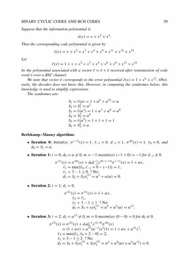
BINARY CYCLIC CODES AND BCH CODES 59
Suppose that the information polynomial is
u(x) = x + x2 + x4.
Then the corresponding code polynomial is given by
v(x) = x + x2 + x3 + x4 + x8 + x11 + x12 + x14.
Letr(x) = 1 + x + x2 + x3 + x4 + x6 + x8 + x11 + x14
be the polynomial associated with a vector r = v + e received after transmission of codeword v over a BSC channel.
We note that vector e corresponds to the error polynomial e(x) = 1 + x6 + x12. Obvi-ously, the decoder does not know this. However, in computing the syndromes below, thisknowledge is used to simplify expressions.
The syndromes are:
S1 = r(α) = 1 + α6 + α12 = α
S2 = S21 = α2
S3 = r(α3) = 1 + α3 + α6 = α8
S4 = S22 = α4
S5 = r(α5) = 1 + 1 + 1 = 1S6 = S2
3 = α
Berlekamp–Massey algorithm:
• Iteration 0: Initialize. σ (−1)(x) = 1, �−1 = 0, d−1 = 1, σ (0)(x) = 1, �0 = 0, andd0 = S1 = α.
• Iteration 1: i = 0, d0 = α �= 0, m = −1 maximizes (−1 + 0) = −1 for d−1 �= 0.
σ (1)(x) = σ (0)(x) + d0d−1−1x(0−(−1))σ (−1)(x) = 1 + αx,
�1 = max{�0, �−1 + 0 − (−1)} = 1,
�1 + 3 − 1 ≤ 0 ? No:d1 = S2 + S1σ
(1)1 = α2 + α(α) = 0.
• Iteration 2: i = 1, d1 = 0,
σ (2)(x) = σ (1)(x) = 1 + αx,
�2 = �1,
�2 + 3 − 1 ≤ 1 ? No:d2 = S3 + s2σ
(1)1 = α8 + α2(α) = α13.
• Iteration 3: i = 2, d2 = α13 �= 0, m = 0 maximizes (0 − 0) = 0 for d0 �= 0.
σ (3)(x) = σ (2)(x) + d2d−10 x(2−0)σ (0)(x)
= (1 + αx) + α13(α−1)x2(1) = 1 + αx + α12x2,
�3 = max{�2, �0 + 2 − 0} = 2,
�3 + 3 − 1 ≤ 2 ? No:d3 = S4 + S3σ
(3)1 + S2σ
(3)2 = α4 + α8(α) + α2(α12) = 0.
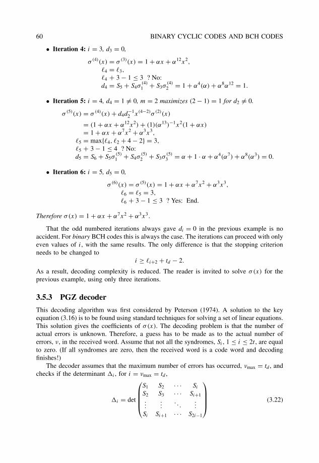
60 BINARY CYCLIC CODES AND BCH CODES
• Iteration 4: i = 3, d3 = 0,
σ (4)(x) = σ (3)(x) = 1 + αx + α12x2,
�4 = �3,
�4 + 3 − 1 ≤ 3 ? No:d4 = S5 + S4σ
(4)1 + S3σ
(4)2 = 1 + α4(α) + α8α12 = 1.
• Iteration 5: i = 4, d4 = 1 �= 0, m = 2 maximizes (2 − 1) = 1 for d2 �= 0.
σ (5)(x) = σ (4)(x) + d4d−12 x(4−2)σ (2)(x)
= (1 + αx + α12x2) + (1)(α13)−1x2(1 + αx)
= 1 + αx + α7x2 + α3x3,
�5 = max{�4, �2 + 4 − 2} = 3,
�5 + 3 − 1 ≤ 4 ? No:d5 = S6 + S5σ
(5)1 + S4σ
(5)2 + S3σ
(5)3 = α + 1 · α + α4(α7) + α8(α3) = 0.
• Iteration 6: i = 5, d5 = 0,
σ (6)(x) = σ (5)(x) = 1 + αx + α7x2 + α3x3,
�6 = �5 = 3,
�6 + 3 − 1 ≤ 3 ? Yes: End.
Therefore σ(x) = 1 + αx + α7x2 + α3x3.
That the odd numbered iterations always gave di = 0 in the previous example is noaccident. For binary BCH codes this is always the case. The iterations can proceed with onlyeven values of i, with the same results. The only difference is that the stopping criterionneeds to be changed to
i ≥ �i+2 + td − 2.
As a result, decoding complexity is reduced. The reader is invited to solve σ(x) for theprevious example, using only three iterations.
3.5.3 PGZ decoder
This decoding algorithm was first considered by Peterson (1974). A solution to the keyequation (3.16) is to be found using standard techniques for solving a set of linear equations.This solution gives the coefficients of σ(x). The decoding problem is that the number ofactual errors is unknown. Therefore, a guess has to be made as to the actual number oferrors, ν, in the received word. Assume that not all the syndromes, Si , 1 ≤ i ≤ 2t , are equalto zero. (If all syndromes are zero, then the received word is a code word and decodingfinishes!)
The decoder assumes that the maximum number of errors has occurred, νmax = td , andchecks if the determinant �i , for i = νmax = td ,
�i = det
S1 S2 · · · Si
S2 S3 · · · Si+1...
.... . .
...
Si Si+1 · · · S2i−1
(3.22)
BINARY CYCLIC CODES AND BCH CODES 61
is equal to zero. If it is, then a smaller number of errors must have occurred. The value of i
is decreased by one, and �i tested again, repeating the procedure if necessary, until i = 1.Otherwise, if �i �= 0, the inverse of the syndrome matrix is computed and the values ofσ1, σ2, . . . , σν are found, where ν = i. In the event that �i = 0, i = 1, 2, . . . , td , decodingis unsuccessful and an uncorrectable error pattern is detected.
Example 3.5.2 In this example, the error-locator polynomial for the BCH (15, 5, 7) codein Example 3.5.1 is found by the PGZ decoding algorithm. First, assume that i = td = 3errors occurred. Then the determinant �3 is computed (using cofactors) as follows:
�3 = det
α α2 α8
α2 α8 α4
α8 α4 1
= α(α8 + α8) + α2(α2 + α12) + α8(α6 + α)
= α2+7 + α8+11 = α14.
Therefore �3 �= 0 and three errors are assumed to have occurred. Substituting the syndromesfound in Example 3.5.1 into the key equation (3.16),
α α2 α8
α2 α8 α4
α8 α4 1
σ3
σ2
σ1
=
α4
1α
. (3.23)
Note that �−13 = α−14 = α−14(1) = α−14α15 = α. The solution to (3.23) is found to be:
σ3 = α det
α4 α2 α8
1 α8 α4
α α4 1
= α(α7 + α12) = α3,
σ2 = α det
α α4 α8
α2 1 α4
α8 α 1
= α(α11 + α) = α7,
σ1 = α det
α α2 α4
α2 α8 1α8 α4 α
= α(α15 + α15 + α15) = α.
It follows that σ(x) = 1 + αx + α7x2 + α3x3, which is the same as the result obtained bythe BMA in example 3.5.1.
3.5.4 Euclidean algorithm
This algorithm is a well-known recursive procedure to find the greatest common divisor(GCD) between two polynomials (or integers). Its application to BCH decoding is describednext. Let the error evaluator polynomial be defined as �(x) = σ(x)S(x), with a syndromepolynomial
S(x) = 1 + S1x + · · · + S2td x2td . (3.24)
From Equation (3.16), it follows that
�(x) = σ(x)S(x) mod x2td+1. (3.25)
62 BINARY CYCLIC CODES AND BCH CODES
The decoding problem can be translated into finding the polynomial �(x) satisfying (3.25).This can be achieved by applying the extended EA to the polynomials r0(x) = x2td+1 andr1(x) = S(x), such that if at the j -th step
rj (x) = aj (x)x2td+1 + bj (x)S(x),
with deg [rj (x)] ≤ td , then �(x) = rj (x) and σi(x) = bj (x). We note that there is nointerest, from the decoding viewpoint, in polynomial ai(x). The extended EA for computingthe GCD of two polynomials is provided below.
Euclidean algorithm: Compute GCD(r0(x),r1(x))
• Inputs: r0(x), r1(x), deg [r0(x)] ≥ deg [r1(x)]
• Initial conditions: a0(x) = 1, b0(x) = 0, a1(x) = 0, b1(x) = 1.
• At step j (j ≥ 2), apply long division to rj−2(x) and rj−1(x),
rj−2(x) = qj (x)rj−1(x) + rj (x), 0 ≤ deg [rj (x)] < deg [rj−1(x)]
and compute
aj (x) = aj−2(x) − qj (x)aj−1(x), bj (x) = bj−2(x) − qj (x)bj−1(x).
• Stop at iteration jlast when deg [rjlast(x)] = 0.
Then GCD(r0(x), r1(x)) = rk(x), k being the largest nonzero integer such that rk(x) �= 0and k < jlast.
Example 3.5.3 In this example, the error-locator polynomial σ(x) for the BCH (15, 5, 7)
code in Example 3.5.1 is computed using the EA.
• Initial conditions
r0(x) = x7,
r1(x) = S(x) = 1 + αx + α2x2 + α8x3 + α4x4 + x5 + αx6,
b0(x) = 0,
b1(x) = 1.
• j = 2:
x7 = (1 + αx + α2x2 + α8x3 + α4x4 + x5 + αx6)(α14x + α13)
+ α8x5 + α12x4 + α11x3 + α13.
r2(x) = α8x5 + α12x4 + α11x3 + α13,
q2(x) = α14x + α13, andb2(x) = b0(x) + q2(x)b1(x) = α14x + α13.
• j = 3:
S(x) = (α8x5 + α12x4 + α11x3 + α13)(α8x + α2) + α14x4 + α3x3 + α2x2 + α11x.
r3(x) = α14x4 + α3x3 + α2x2 + α11x,
q3(x) = α8x + α2, andb3(x) = b1(x) + q3(x)b2(x) = α7x2 + α11x.
BINARY CYCLIC CODES AND BCH CODES 63
• j = 4:
α8x5 + α12x4 + α11x3 + α13 = (α14x4 + α3x3 + α2x2 + α11x)(α9x) + α5x + α13.
r4(x) = α5x + α13,
q4(x) = α9x, andb4(x) = b2(x) + q4(x)b3(x) = αx3 + α5x2 + α14x + α13.
Because deg[r4(x)] = 1 ≤ 3, the algorithm stops.It follows that σ(x) = b4(x) = α13(1 + αx + α7x2 + α3x3), which has the same roots
as the polynomial obtained by the BMA and PGZ decoder (see Example 3.5.4 below), anddiffers only by a constant factor.9
As the example above illustrates, generally the error-locator polynomial obtained withthe EA will differ from that obtained by BMA or PGZ decoding by a constant factor. Indecoding, however, the roots of these polynomials are of interest and not their coefficients,and thus any of the three methods discussed so far can be used to determine σ(x).
3.5.5 Chien search and error correction
To find the roots of σ(x), a simple trial-and-error procedure – called Chien search – isperformed. All nonzero elements β of GF(2m) are generated in sequence 1, α, α2, . . . andthe condition σ(β−1) = 0 tested. This process is easy to implement in hardware. Moreover,finding roots (factoring) of polynomials over GF(2m) is a challenging mathematical problemthat remains to be solved.
For binary BCH codes, once the error locations j1, . . . , jν are known, the correspondingbits in the received word are complemented
vj�= vj�
+ 1, 1 ≤ � ≤ ν
and the estimated code word v(x) generated.
Example 3.5.4 In Example 3.5.1, the roots of σ(x) are 1, α9 = α−6 and α3 = α−12. Statedin a different way, σ(x) factors as
σ(x) = (1 + x)(1 + α6x)(1 + α12x).
Consequently, the estimated error polynomial is e(x) = 1 + x6 + x12, and
r(x) = x + x2 + x3 + x4 + x6 + x8 + x11 + x14.
Three errors have been corrected.
3.5.6 Errors-and-erasures decoding
There are many situations in which a decision on a received symbol is not consideredreliable. An example is binary transmission over an AWGN channel, with bits mapped to
9The normalized polynomial σnorm(x) = σ−10 σ(x) is identical to the one obtained in the BMA and PGZ
procedures.
64 BINARY CYCLIC CODES AND BCH CODES
real amplitudes, for example, binary phase shift keying (BPSK) with 0 �→ +1 and 1 �→ −1.If the received values are too close to zero, then it may be more advantageous, from theviewpoint of minimizing the probability of a decoding error, to declare a “no-decision”. Insuch a case, the received symbol is “erased” and it is called an erasure.10 Declaring erasuresis the simplest form of soft-decision, which will be the focus of attention in Chapter 7.
Introduction of erasures has the advantage, with respect to errors-only decoding, that thepositions are known to the decoder. Let d be the minimum distance of a code, ν be thenumber of errors and µ be the number of erasures contained in a received word. Then,the minimum Hamming distance between code words is reduced to at least d − µ in thenonerased positions. It follows that the error-correcting capability is �(d − µ − 1)/2� andthe following relation holds:
d > 2ν + µ. (3.26)
The above inequality is intuitively satisfying: for a fixed minimum distance, it is twice asdifficult to correct an error as it is to correct an erasure, because the erased positions arealready known.
For binary linear codes, including binary BCH codes, erasures can be corrected withthe following method:
1. Place zeros in all erased positions and decode to a code word v0(x).
2. Place ones in all erased positions and decode to a code word v1(x).
3. Choose as decoded word the closest vj (x) to the received word r(x) in the nonerasedpositions, j = 0, 1. (Alternatively, choose the code word that requires the smallestnumber of error corrections, (Michelson and Levesque 1985).)
As a result, erasures can be corrected with two rounds of errors-only decoding.
Example 3.5.5 Consider a binary cyclic Hamming (7, 4, 3) code with
g(x) = 1 + x + x3,
and the Galois field GF(23) with a primitive element α such that p(α) = 1 + α + α3 = 0.Suppose that v(x) = x + x2 + x4 is transmitted and that µ = 2 erasures are introduced atthe receiver. Since d = 3 > µ, these erasures can be corrected. Let
r(x) = f + x + x2 + f x3 + x4
be the polynomial associated with the received vector, where f denotes an erasure.
First decoding (f = 0):r0(x) = x + x2 + x4. The syndromes are S1 = r0(α) = 0, and S2 = S2
1 = 0. Therefore,v0(x) = r0(x) = x + x2 + x4.
Second decoding (f = 1):r1(x) = 1 + x + x2 + x3 + x4. The syndromes are S1 = α and S2 = α2. Equation (3.16)
in this case is: ασ1 = α2. Therefore σ(x) = 1 + αx, e(x) = x and
v1(x) = r1(x) + e(x) = 1 + x2 + x3 + x4,
10In information theoretical terms, the BSC channel becomes a two-input three-output binary erasure channel(BEC) (Cover and Thomas 1991).
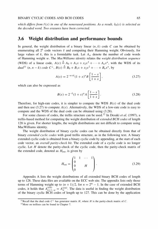
BINARY CYCLIC CODES AND BCH CODES 65
which differs from r(x) in one of the nonerased positions. As a result, v0(x) is selected asthe decoded word. Two erasures have been corrected.
3.6 Weight distribution and performance bounds
In general, the weight distribution of a binary linear (n, k) code C can be obtained byenumerating all 2k code vectors v and computing their Hamming weight. Obviously, forlarge values of k, this is a formidable task. Let Aw denote the number of code wordsof Hamming weight w. The MacWilliams identity relates the weight distribution sequence
(WDS) of a linear code, A(x)�= A0 + A1x + x2x
2 + · · · + Anxn, with the WDS of its
dual11 (n, n − k) code C⊥, B(x)�= B0 + B1x + x2x
2 + · · · + Bnxn, by
A(x) = 2−n+k(1 + x)nB
[1 − x
1 + x
], (3.27)
which can also be expressed as
B(x) = 2−k(1 + x)nA
[1 − x
1 + x
]. (3.28)
Therefore, for high-rate codes, it is simpler to compute the WDS B(x) of the dual codeand then use (3.27) to compute A(x). Alternatively, the WDS of a low-rate code is easy tocompute and the WDS of the dual code can be obtained using (3.28).
For some classes of codes, the trellis structure can be used.12 In Desaki et al. (1997), atrellis-based method for computing the weight distribution of extended BCH codes of length128 is given. For shorter lengths, the weight distributions are not difficult to compute usingMacWilliams identity.
The weight distribution of binary cyclic codes can be obtained directly from that ofbinary extended cyclic codes with good trellis structure, as in the following text. A binaryextended cyclic code is obtained from a binary cyclic code by appending, at the start of eachcode vector, an overall parity-check bit. The extended code of a cyclic code is no longercyclic. Let H denote the parity-check of the cyclic code, then the parity-check matrix ofthe extended code, denoted as Hext, is given by
Hext =
1 1 · · · 100 H
0
. (3.29)
Appendix A lists the weight distributions of all extended binary BCH codes of lengthup to 128. These data files are available on the ECC web site. The appendix lists only thoseterms of Hamming weight up to (n + 1)/2, for n = 2m − 1. In the case of extended BCHcodes, it holds that A
(ext)n+1−w = A(ext)
w . The data is useful in finding the weight distributionof the binary cyclic BCH codes of length up to 127. This can be done by the application
11Recall that the dual code C⊥ has generator matrix H , where H is the parity-check matrix of C.12More on trellises can be found in Chapter 7.
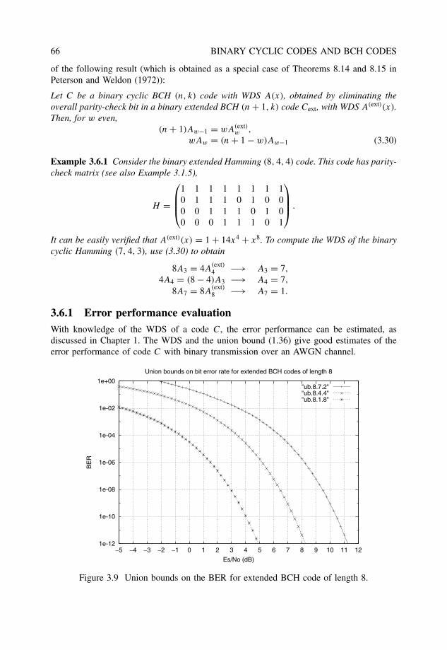
66 BINARY CYCLIC CODES AND BCH CODES
of the following result (which is obtained as a special case of Theorems 8.14 and 8.15 inPeterson and Weldon (1972)):
Let C be a binary cyclic BCH (n, k) code with WDS A(x), obtained by eliminating theoverall parity-check bit in a binary extended BCH (n + 1, k) code Cext, with WDS A(ext)(x).Then, for w even,
(n + 1)Aw−1 = wA(ext)w ,
wAw = (n + 1 − w)Aw−1 (3.30)
Example 3.6.1 Consider the binary extended Hamming (8, 4, 4) code. This code has parity-check matrix (see also Example 3.1.5),
H =
1 1 1 1 1 1 1 10 1 1 1 0 1 0 00 0 1 1 1 0 1 00 0 0 1 1 1 0 1
.
It can be easily verified that A(ext)(x) = 1 + 14x4 + x8. To compute the WDS of the binarycyclic Hamming (7, 4, 3), use (3.30) to obtain
8A3 = 4A(ext)4 −→ A3 = 7,
4A4 = (8 − 4)A3 −→ A4 = 7,
8A7 = 8A(ext)8 −→ A7 = 1.
3.6.1 Error performance evaluationWith knowledge of the WDS of a code C, the error performance can be estimated, asdiscussed in Chapter 1. The WDS and the union bound (1.36) give good estimates of theerror performance of code C with binary transmission over an AWGN channel.
1e-12
1e-10
1e-08
1e-06
1e-04
1e-02
1e+00
−5 −4 −3 −2 −1 0 1 2 3 4 5 6 7 8 9 10 11 12
BE
R
Es/No (dB)
Union bounds on bit error rate for extended BCH codes of length 8
"ub.8.7.2""ub.8.4.4""ub.8.1.8"
Figure 3.9 Union bounds on the BER for extended BCH code of length 8.
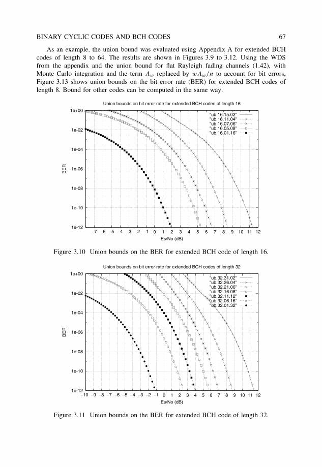
BINARY CYCLIC CODES AND BCH CODES 67
As an example, the union bound was evaluated using Appendix A for extended BCHcodes of length 8 to 64. The results are shown in Figures 3.9 to 3.12. Using the WDSfrom the appendix and the union bound for flat Rayleigh fading channels (1.42), withMonte Carlo integration and the term Aw replaced by wAw/n to account for bit errors,Figure 3.13 shows union bounds on the bit error rate (BER) for extended BCH codes oflength 8. Bound for other codes can be computed in the same way.
1e-12
1e-10
1e-08
1e-06
1e-04
1e-02
1e+00
−7 −6 −5 −4 −3 −2 −1 0 1 2 3 4 5 6 7 8 9 10 11 12
BE
R
Es/No (dB)
Union bounds on bit error rate for extended BCH codes of length 16
"ub.16.15.02""ub.16.11.04""ub.16.07.06""ub.16.05.08""ub.16.01.16"
Figure 3.10 Union bounds on the BER for extended BCH code of length 16.
1e-12
1e-10
1e-08
1e-06
1e-04
1e-02
1e+00
−10 −9 −8 −7 −6 −5 −4 −3 −2 −1 0 1 2 3 4 5 6 7 8 9 10 11 12
BE
R
Es/No (dB)
Union bounds on bit error rate for extended BCH codes of length 32
"ub.32.31.02""ub.32.26.04""ub.32.21.06""ub.32.16.08""ub.32.11.12""ub.32.06.16""ub.32.01.32"
Figure 3.11 Union bounds on the BER for extended BCH code of length 32.
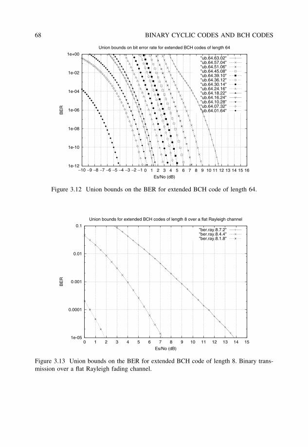
68 BINARY CYCLIC CODES AND BCH CODES
1e-12
1e-10
1e-08
1e-06
1e-04
1e-02
1e+00
−10 −9 −8 −7 −6 −5 −4 −3 −2 −1 0 1 2 3 4 5 6 7 8 9 10 11 12 13 14 15 16
BE
R
Es/No (dB)
Union bounds on bit error rate for extended BCH codes of length 64
"ub.64.63.02""ub.64.57.04""ub.64.51.06""ub.64.45.08""ub.64.39.10""ub.64.36.12""ub.64.30.14""ub.64.24.16""ub.64.18.22""ub.64.16.24""ub.64.10.28""ub.64.07.32""ub.64.01.64"
Figure 3.12 Union bounds on the BER for extended BCH code of length 64.
1e-05
0.0001
0.001
0.01
0.1
0 1 2 3 4 5 6 7 8 9 10 11 12 13 14 15
BE
R
Es/No (dB)
Union bounds for extended BCH codes of length 8 over a flat Rayleigh channel
"ber.ray.8.7.2""ber.ray.8.4.4""ber.ray.8.1.8"
Figure 3.13 Union bounds on the BER for extended BCH code of length 8. Binary trans-mission over a flat Rayleigh fading channel.
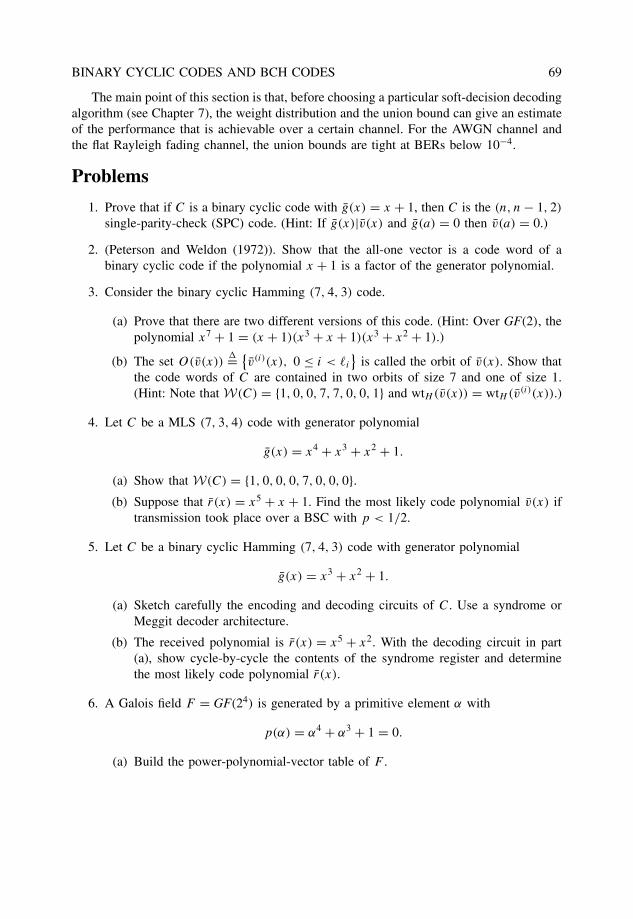
BINARY CYCLIC CODES AND BCH CODES 69
The main point of this section is that, before choosing a particular soft-decision decodingalgorithm (see Chapter 7), the weight distribution and the union bound can give an estimateof the performance that is achievable over a certain channel. For the AWGN channel andthe flat Rayleigh fading channel, the union bounds are tight at BERs below 10−4.
Problems
1. Prove that if C is a binary cyclic code with g(x) = x + 1, then C is the (n, n − 1, 2)
single-parity-check (SPC) code. (Hint: If g(x)|v(x) and g(a) = 0 then v(a) = 0.)
2. (Peterson and Weldon (1972)). Show that the all-one vector is a code word of abinary cyclic code if the polynomial x + 1 is a factor of the generator polynomial.
3. Consider the binary cyclic Hamming (7, 4, 3) code.
(a) Prove that there are two different versions of this code. (Hint: Over GF(2), thepolynomial x7 + 1 = (x + 1)(x3 + x + 1)(x3 + x2 + 1).)
(b) The set O(v(x))�= {
v(i)(x), 0 ≤ i < �i
}is called the orbit of v(x). Show that
the code words of C are contained in two orbits of size 7 and one of size 1.(Hint: Note that W(C) = {1, 0, 0, 7, 7, 0, 0, 1} and wtH (v(x)) = wtH (v(i)(x)).)
4. Let C be a MLS (7, 3, 4) code with generator polynomial
g(x) = x4 + x3 + x2 + 1.
(a) Show that W(C) = {1, 0, 0, 0, 7, 0, 0, 0}.(b) Suppose that r(x) = x5 + x + 1. Find the most likely code polynomial v(x) if
transmission took place over a BSC with p < 1/2.
5. Let C be a binary cyclic Hamming (7, 4, 3) code with generator polynomial
g(x) = x3 + x2 + 1.
(a) Sketch carefully the encoding and decoding circuits of C. Use a syndrome orMeggit decoder architecture.
(b) The received polynomial is r(x) = x5 + x2. With the decoding circuit in part(a), show cycle-by-cycle the contents of the syndrome register and determinethe most likely code polynomial r(x).
6. A Galois field F = GF(24) is generated by a primitive element α with
p(α) = α4 + α3 + 1 = 0.
(a) Build the power-polynomial-vector table of F .

70 BINARY CYCLIC CODES AND BCH CODES
(b) Find the value of X in F in the following expressions:
(i) α5X = 1
(ii) (α2 + α9)3 X = α10
(i) α11 + X = α
(c) Determine the cyclotomic sets modulo 15 and use them to find the minimalpolynomials φ3(x) and φ5(x).
7. Find the generator polynomial of a (1,2)-order EG code of length 63.
8. Show that the (0,2)-order EG code of length 15 is a binary BCH (15, 5, 7) code.
9. Show that the (1,1)-order EG code of length 15 is a binary BCH (15, 7, 5) code.
10. Find the generator polynomial of a (1,2)-order PG code of length 21. This code is abinary (21, 11) difference-set code. See Lin and Costello (2005).
11. (MacWilliams and Sloane (1977)). Use the BCH bound to show that the dual of abinary cyclic Hamming code, a binary (2m − 1, m, d) simplex code, has the minimumdistance d = 2m−1.
12. (MacWilliams and Sloane (1977)). A code C is reversible if (c0, c1, . . . , cn−1) ∈ C
implies (cn−1, cn−2, . . . , c0) ∈ C. For example, the code C = {000, 110, 101, 011} isreversible. Show that the BCH code with b = −t and designed distance d = 2t + 2is reversible.
13. Let C be a binary cyclic triple-error-correcting BCH (15, 5, 7) code.
(a) Using the field F in problem 2, determine the generator polynomial of C.
(b) The information message is u = (10101). Determine the corresponding codepolynomial v(x) in C.
(c) Suppose that the error polynomial is e(x) = x12 + x5 + x. Compute the receivedpolynomial r(x) = v(x) + e(x). Using r(x), do the following:
(i) Determine the syndromes Si = r(αi), 1 ≤ i ≤ 6.
(ii) Determine the error-locator polynomial σ(x).
(iii) Determine the error locations αji , i = 1, 2, 3.
(iv) Correct the errors in r(x) by constructing the estimated error polynomiale(x) and the estimated code polynomial c(x) = r(x) + e(x). Verify thaterrors have been corrected successfully.
14. Let Ci�= {i, 2i, 4i, . . . , 2mi−1i} mod 2m − 1 be a cyclotomic set, where i is the small-
est integer in Ci . Prove that i cannot be an even number.
15. Factor the polynomials (x4 + 1) and (x5 + 1) over GF(2).
16. Prove that for a binary BCH code, the following relation between syndromes holds:S2i = S2
i .
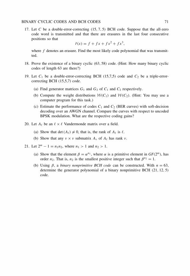
BINARY CYCLIC CODES AND BCH CODES 71
17. Let C be a double-error-correcting (15, 7, 5) BCH code. Suppose that the all-zerocode word is transmitted and that there are erasures in the last four consecutivepositions so that
r(x) = f + f x + f x2 + f x3,
where f denotes an erasure. Find the most likely code polynomial that was transmit-ted.
18. Prove the existence of a binary cyclic (63, 58) code. (Hint: How many binary cycliccodes of length 63 are there?)
19. Let C1 be a double-error-correcting BCH (15,7,5) code and C2 be a triple-error-correcting BCH (15,5,7) code.
(a) Find generator matrices G1 and G2 of C1 and C2 respectively.
(b) Compute the weight distributions W(C1) and W(C2). (Hint: You may use acomputer program for this task.)
(c) Estimate the performance of codes C1 and C2 (BER curves) with soft-decisiondecoding over an AWGN channel. Compare the curves with respect to uncodedBPSK modulation. What are the respective coding gains?
20. Let A� be an � × � Vandermonde matrix over a field.
(a) Show that det (A�) �= 0, that is, the rank of A� is �.
(b) Show that any ν × ν submatrix Aν of A� has rank ν.
21. Let 2m − 1 = n1n2, where n1 > 1 and n2 > 1.
(a) Show that the element β = αn1 , where α is a primitive element in GF(2m), hasorder n2. That is, n2 is the smallest positive integer such that βn2 = 1.
(b) Using β, a binary nonprimitive BCH code can be constructed. With n = 63,determine the generator polynomial of a binary nonprimitive BCH (21, 12, 5)
code.
4
Nonbinary BCH codes:Reed–Solomon codes
In this chapter, one of the most celebrated class of ECC schemes is introduced andtheir encoding and decoding algorithms explained. Reed–Solomon (RS) codes have foundnumerous applications in digital storage and communication systems. Examples include thefamous RS (255, 223, 33) code for NASA space communications, shortened RS codes overGF(28) for CD-ROM, DVD and Terrestrial Digital HDTV transmission applications, anextended RS (128, 122, 7) code over GF(27) for cable modems, among many others.
4.1 RS codes as polynomial codesSimilar to Reed–Muller (RM) codes, RS codes can be defined as code words with compo-nents equal to the evaluation of a certain polynomial. As a matter of fact, this was the waythat RS codes were originally defined by Reed and Solomon in Reed and Solomon (1960).RM codes, finite-geometry codes (Lin and Costello 2005) and RS codes are all membersof a large class of codes: Polynomial codes (Peterson and Weldon 1972), which are closelyrelated to algebraic-geometry (AG) codes (Pretzel 1998). Let
u(x) = u0 + u1x + · · · + uk−1xk−1 (4.1)
be an information polynomial, with ui ∈ GF(2m), 1 ≤ i < k. Clearly, there are 2mk suchpolynomials. By evaluating (4.1) over the nonzero elements of GF(2m), a code word in anRS (2m − 1, k, d) code of length 2m is obtained,
v = (u(1) u(α) u(α2) · · · u(α2m−2)
). (4.2)
4.2 From binary BCH to RS codesRS codes can also be interpreted as nonbinary BCH codes. That is, RS codes are BCHcodes in which the values of the code coefficient are taken from GF(2m). In particular,
The Art of Error Correcting Coding, Second Edition Robert H. Morelos-Zaragoza 2006 John Wiley & Sons, Ltd. ISBN: 0-470-01558-6
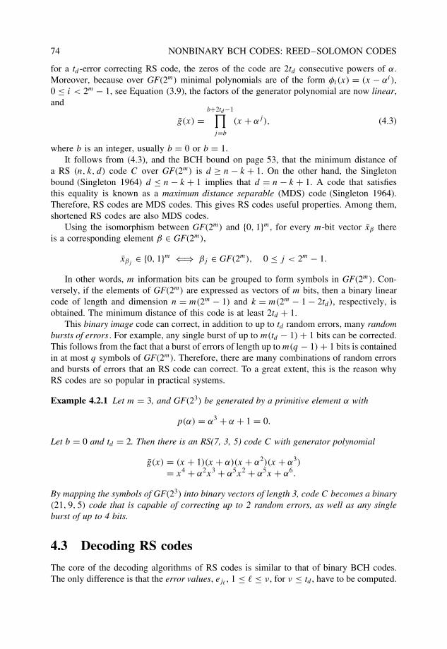
74 NONBINARY BCH CODES: REED–SOLOMON CODES
for a td -error correcting RS code, the zeros of the code are 2td consecutive powers of α.Moreover, because over GF(2m) minimal polynomials are of the form φi(x) = (x − αi),0 ≤ i < 2m − 1, see Equation (3.9), the factors of the generator polynomial are now linear,and
g(x) =b+2td−1∏
j=b
(x + αj), (4.3)
where b is an integer, usually b = 0 or b = 1.It follows from (4.3), and the BCH bound on page 53, that the minimum distance of
a RS (n, k, d) code C over GF(2m) is d ≥ n − k + 1. On the other hand, the Singletonbound (Singleton 1964) d ≤ n − k + 1 implies that d = n − k + 1. A code that satisfiesthis equality is known as a maximum distance separable (MDS) code (Singleton 1964).Therefore, RS codes are MDS codes. This gives RS codes useful properties. Among them,shortened RS codes are also MDS codes.
Using the isomorphism between GF(2m) and {0, 1}m, for every m-bit vector xβ thereis a corresponding element β ∈ GF(2m),
xβj∈ {0, 1}m ⇐⇒ βj ∈ GF(2m), 0 ≤ j < 2m − 1.
In other words, m information bits can be grouped to form symbols in GF(2m). Con-versely, if the elements of GF(2m) are expressed as vectors of m bits, then a binary linearcode of length and dimension n = m(2m − 1) and k = m(2m − 1 − 2td ), respectively, isobtained. The minimum distance of this code is at least 2td + 1.
This binary image code can correct, in addition to up to td random errors, many randombursts of errors . For example, any single burst of up to m(td − 1) + 1 bits can be corrected.This follows from the fact that a burst of errors of length up to m(q − 1) + 1 bits is containedin at most q symbols of GF(2m). Therefore, there are many combinations of random errorsand bursts of errors that an RS code can correct. To a great extent, this is the reason whyRS codes are so popular in practical systems.
Example 4.2.1 Let m = 3, and GF(23) be generated by a primitive element α with
p(α) = α3 + α + 1 = 0.
Let b = 0 and td = 2. Then there is an RS(7, 3, 5) code C with generator polynomial
g(x) = (x + 1)(x + α)(x + α2)(x + α3)
= x4 + α2x3 + α5x2 + α5x + α6.
By mapping the symbols of GF(23) into binary vectors of length 3, code C becomes a binary(21, 9, 5) code that is capable of correcting up to 2 random errors, as well as any singleburst of up to 4 bits.
4.3 Decoding RS codes
The core of the decoding algorithms of RS codes is similar to that of binary BCH codes.The only difference is that the error values, ej�
, 1 ≤ � ≤ ν, for ν ≤ td , have to be computed.
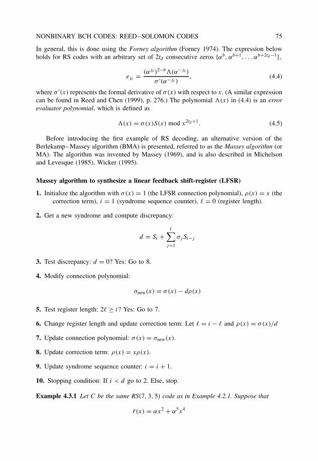
NONBINARY BCH CODES: REED–SOLOMON CODES 75
In general, this is done using the Forney algorithm (Forney 1974). The expression belowholds for RS codes with an arbitrary set of 2td consecutive zeros {αb, αb+1, . . . αb+2td−1},
ej�= (αj�)2−b�(α−j�)
σ ′(α−j�), (4.4)
where σ ′(x) represents the formal derivative of σ(x) with respect to x. (A similar expressioncan be found in Reed and Chen (1999), p. 276.) The polynomial �(x) in (4.4) is an errorevaluator polynomial, which is defined as
�(x) = σ(x)S(x) mod x2td+1. (4.5)
Before introducing the first example of RS decoding, an alternative version of theBerlekamp–Massey algorithm (BMA) is presented, referred to as the Massey algorithm (orMA). The algorithm was invented by Massey (1969), and is also described in Michelsonand Levesque (1985), Wicker (1995).
Massey algorithm to synthesize a linear feedback shift-register (LFSR)
1. Initialize the algorithm with σ(x) = 1 (the LFSR connection polynomial), ρ(x) = x (thecorrection term), i = 1 (syndrome sequence counter), � = 0 (register length).
2. Get a new syndrome and compute discrepancy:
d = Si +�∑
j=1
σjSi−j
3. Test discrepancy: d = 0? Yes: Go to 8.
4. Modify connection polynomial:
σnew(x) = σ(x) − dρ(x)
5. Test register length: 2� ≥ i? Yes: Go to 7.
6. Change register length and update correction term: Let � = i − � and ρ(x) = σ(x)/d
7. Update connection polynomial: σ(x) = σnew(x).
8. Update correction term: ρ(x) = xρ(x).
9. Update syndrome sequence counter: i = i + 1.
10. Stopping condition: If i < d go to 2. Else, stop.
Example 4.3.1 Let C be the same RS(7, 3, 5) code as in Example 4.2.1. Suppose that
r(x) = αx2 + α5x4
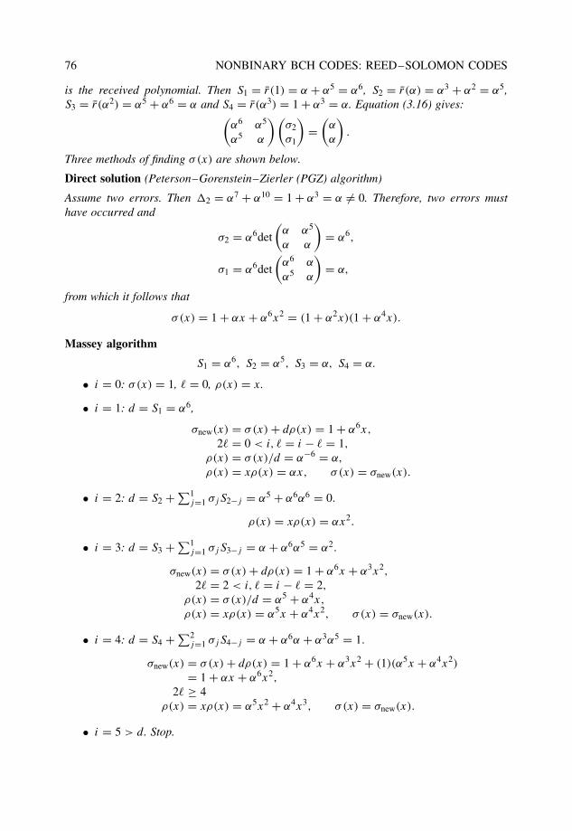
76 NONBINARY BCH CODES: REED–SOLOMON CODES
is the received polynomial. Then S1 = r(1) = α + α5 = α6, S2 = r(α) = α3 + α2 = α5,S3 = r(α2) = α5 + α6 = α and S4 = r(α3) = 1 + α3 = α. Equation (3.16) gives:(
α6 α5
α5 α
)(σ2
σ1
)=
(α
α
).
Three methods of finding σ(x) are shown below.
Direct solution (Peterson–Gorenstein–Zierler (PGZ) algorithm)
Assume two errors. Then 2 = α7 + α10 = 1 + α3 = α �= 0. Therefore, two errors musthave occurred and
σ2 = α6det
(α α5
α α
)= α6,
σ1 = α6det
(α6 α
α5 α
)= α,
from which it follows that
σ(x) = 1 + αx + α6x2 = (1 + α2x)(1 + α4x).
Massey algorithm
S1 = α6, S2 = α5, S3 = α, S4 = α.
• i = 0: σ(x) = 1, � = 0, ρ(x) = x.
• i = 1: d = S1 = α6,
σnew(x) = σ(x) + dρ(x) = 1 + α6x,
2� = 0 < i, � = i − � = 1,
ρ(x) = σ(x)/d = α−6 = α,
ρ(x) = xρ(x) = αx, σ (x) = σnew(x).
• i = 2: d = S2 + ∑1j=1 σjS2−j = α5 + α6α6 = 0.
ρ(x) = xρ(x) = αx2.
• i = 3: d = S3 + ∑1j=1 σjS3−j = α + α6α5 = α2.
σnew(x) = σ(x) + dρ(x) = 1 + α6x + α3x2,
2� = 2 < i, � = i − � = 2,
ρ(x) = σ(x)/d = α5 + α4x,
ρ(x) = xρ(x) = α5x + α4x2, σ (x) = σnew(x).
• i = 4: d = S4 + ∑2j=1 σjS4−j = α + α6α + α3α5 = 1.
σnew(x) = σ(x) + dρ(x) = 1 + α6x + α3x2 + (1)(α5x + α4x2)
= 1 + αx + α6x2,
2� ≥ 4ρ(x) = xρ(x) = α5x2 + α4x3, σ (x) = σnew(x).
• i = 5 > d. Stop.
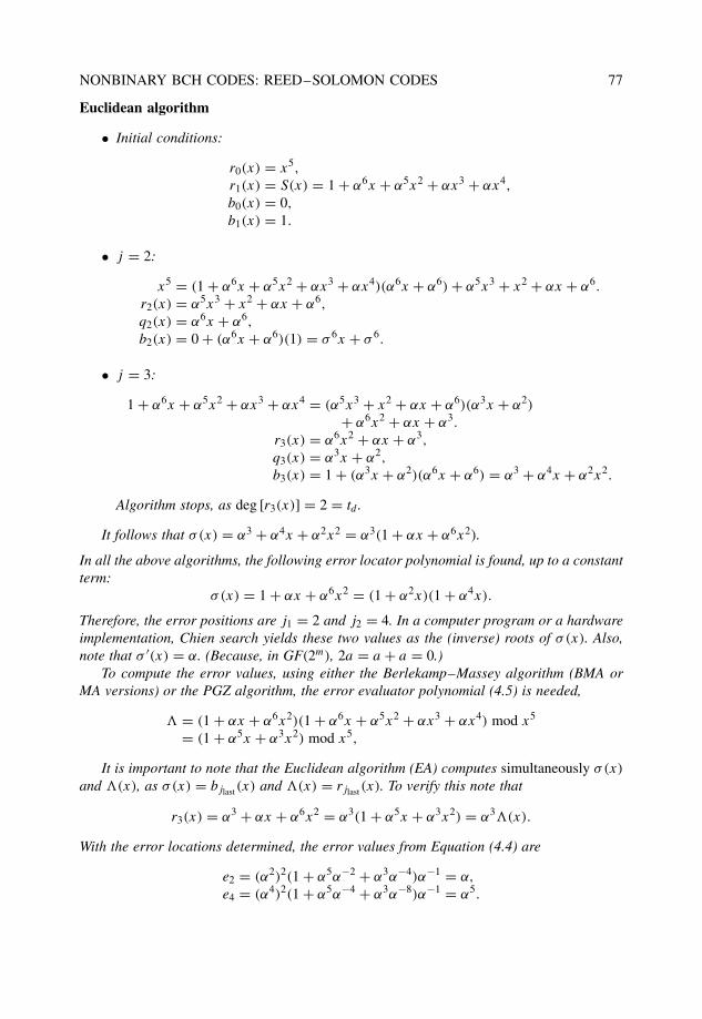
NONBINARY BCH CODES: REED–SOLOMON CODES 77
Euclidean algorithm
• Initial conditions:
r0(x) = x5,
r1(x) = S(x) = 1 + α6x + α5x2 + αx3 + αx4,
b0(x) = 0,
b1(x) = 1.
• j = 2:
x5 = (1 + α6x + α5x2 + αx3 + αx4)(α6x + α6) + α5x3 + x2 + αx + α6.
r2(x) = α5x3 + x2 + αx + α6,
q2(x) = α6x + α6,
b2(x) = 0 + (α6x + α6)(1) = σ 6x + σ 6.
• j = 3:
1 + α6x + α5x2 + αx3 + αx4 = (α5x3 + x2 + αx + α6)(α3x + α2)
+ α6x2 + αx + α3.
r3(x) = α6x2 + αx + α3,
q3(x) = α3x + α2,
b3(x) = 1 + (α3x + α2)(α6x + α6) = α3 + α4x + α2x2.
Algorithm stops, as deg [r3(x)] = 2 = td .
It follows that σ(x) = α3 + α4x + α2x2 = α3(1 + αx + α6x2).
In all the above algorithms, the following error locator polynomial is found, up to a constantterm:
σ(x) = 1 + αx + α6x2 = (1 + α2x)(1 + α4x).
Therefore, the error positions are j1 = 2 and j2 = 4. In a computer program or a hardwareimplementation, Chien search yields these two values as the (inverse) roots of σ(x). Also,note that σ ′(x) = α. (Because, in GF(2m), 2a = a + a = 0.)
To compute the error values, using either the Berlekamp–Massey algorithm (BMA orMA versions) or the PGZ algorithm, the error evaluator polynomial (4.5) is needed,
� = (1 + αx + α6x2)(1 + α6x + α5x2 + αx3 + αx4) mod x5
= (1 + α5x + α3x2) mod x5,
It is important to note that the Euclidean algorithm (EA) computes simultaneously σ(x)
and �(x), as σ(x) = bjlast(x) and �(x) = rjlast(x). To verify this note that
r3(x) = α3 + αx + α6x2 = α3(1 + α5x + α3x2) = α3�(x).
With the error locations determined, the error values from Equation (4.4) are
e2 = (α2)2(1 + α5α−2 + α3α−4)α−1 = α,
e4 = (α4)2(1 + α5α−4 + α3α−8)α−1 = α5.
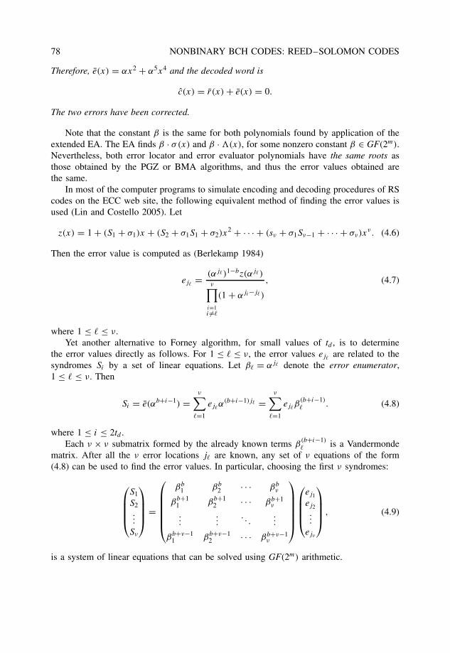
78 NONBINARY BCH CODES: REED–SOLOMON CODES
Therefore, e(x) = αx2 + α5x4 and the decoded word is
c(x) = r(x) + e(x) = 0.
The two errors have been corrected.
Note that the constant β is the same for both polynomials found by application of theextended EA. The EA finds β · σ(x) and β · �(x), for some nonzero constant β ∈ GF(2m).Nevertheless, both error locator and error evaluator polynomials have the same roots asthose obtained by the PGZ or BMA algorithms, and thus the error values obtained arethe same.
In most of the computer programs to simulate encoding and decoding procedures of RScodes on the ECC web site, the following equivalent method of finding the error values isused (Lin and Costello 2005). Let
z(x) = 1 + (S1 + σ1)x + (S2 + σ1S1 + σ2)x2 + · · · + (sν + σ1Sν−1 + · · · + σν)x
ν. (4.6)
Then the error value is computed as (Berlekamp 1984)
ej�= (αj�)1−bz(αj�)
ν∏i=1i �=�
(1 + αji−j�)
, (4.7)
where 1 ≤ � ≤ ν.Yet another alternative to Forney algorithm, for small values of td , is to determine
the error values directly as follows. For 1 ≤ � ≤ ν, the error values ej�are related to the
syndromes Si by a set of linear equations. Let β� = αj� denote the error enumerator,1 ≤ � ≤ ν. Then
Si = e(αb+i−1) =ν∑
�=1
ej�α(b+i−1)j� =
ν∑�=1
ej�β
(b+i−1)� . (4.8)
where 1 ≤ i ≤ 2td .Each ν × ν submatrix formed by the already known terms β
(b+i−1)� is a Vandermonde
matrix. After all the ν error locations j� are known, any set of ν equations of the form(4.8) can be used to find the error values. In particular, choosing the first ν syndromes:
S1
S2...
Sν
=
βb1 βb
2 · · · βbν
βb+11 βb+1
2 · · · βb+1ν
......
. . ....
βb+ν−11 βb+ν−1
2 · · · βb+ν−1ν
ej1
ej2...
ejν
, (4.9)
is a system of linear equations that can be solved using GF(2m) arithmetic.
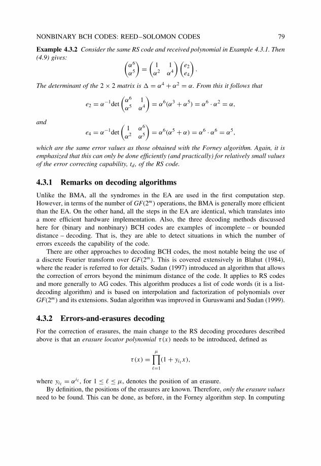
NONBINARY BCH CODES: REED–SOLOMON CODES 79
Example 4.3.2 Consider the same RS code and received polynomial in Example 4.3.1. Then(4.9) gives: (
α6
α5
)=
(1 1α2 α4
)(e2
e4
).
The determinant of the 2 × 2 matrix is = α4 + α2 = α. From this it follows that
e2 = α−1det
(α6 1α5 α4
)= α6(α3 + α5) = α6 · α2 = α,
and
e4 = α−1det
(1 α6
α2 α5
)= α6(α5 + α) = α6 · α6 = α5,
which are the same error values as those obtained with the Forney algorithm. Again, it isemphasized that this can only be done efficiently (and practically) for relatively small valuesof the error correcting capability, td , of the RS code.
4.3.1 Remarks on decoding algorithms
Unlike the BMA, all the syndromes in the EA are used in the first computation step.However, in terms of the number of GF(2m) operations, the BMA is generally more efficientthan the EA. On the other hand, all the steps in the EA are identical, which translates intoa more efficient hardware implementation. Also, the three decoding methods discussedhere for (binary and nonbinary) BCH codes are examples of incomplete – or boundeddistance – decoding. That is, they are able to detect situations in which the number oferrors exceeds the capability of the code.
There are other approaches to decoding BCH codes, the most notable being the use ofa discrete Fourier transform over GF(2m). This is covered extensively in Blahut (1984),where the reader is referred to for details. Sudan (1997) introduced an algorithm that allowsthe correction of errors beyond the minimum distance of the code. It applies to RS codesand more generally to AG codes. This algorithm produces a list of code words (it is a list-decoding algorithm) and is based on interpolation and factorization of polynomials overGF(2m) and its extensions. Sudan algorithm was improved in Guruswami and Sudan (1999).
4.3.2 Errors-and-erasures decoding
For the correction of erasures, the main change to the RS decoding procedures describedabove is that an erasure locator polynomial τ (x) needs to be introduced, defined as
τ (x) =µ∏
�=1
(1 + yi�x),
where yi� = αi� , for 1 ≤ � ≤ µ, denotes the position of an erasure.By definition, the positions of the erasures are known. Therefore, only the erasure values
need to be found. This can be done, as before, in the Forney algorithm step. In computing
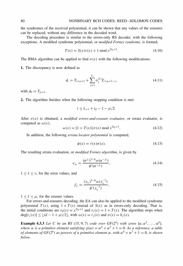
80 NONBINARY BCH CODES: REED–SOLOMON CODES
the syndromes of the received polynomial, it can be shown that any values of the erasurescan be replaced, without any difference in the decoded word.
The decoding procedure is similar to the errors-only RS decoder, with the followingexceptions. A modified syndrome polynomial, or modified Forney syndrome, is formed,
T (x) = S(x)τ (x) + 1 mod x2td+1. (4.10)
The BMA algorithm can be applied to find σ(x) with the following modifications:
1. The discrepancy is now defined as
di = Ti+µ+1 +�i∑
j=1
σ(i)j Ti+µ+1−j , (4.11)
with d0 = Tµ+1.
2. The algorithm finishes when the following stopping condition is met:
i ≥ li+1 + td − 1 − µ/2.
After σ(x) is obtained, a modified errors-and-erasure evaluator, or errata evaluator, iscomputed as ω(x),
ω(x) = [1 + T (x)] σ(x) mod x2td+1. (4.12)
In addition, the following errata locator polynomial is computed,
φ(x) = τ (x)σ (x). (4.13)
The resulting errata evaluation, or modified Forney algorithm, is given by
ej�= (αj�)2−bω(α−j�)
φ′(α−j�), (4.14)
1 ≤ � ≤ ν, for the error values, and
fi� = (yi�)2−bω(y−1
i�)
φ′(y−1i�
), (4.15)
1 ≤ � ≤ µ, for the erasure values.For errors-and-erasures decoding, the EA can also be applied to the modified syndrome
polynomial T (x), using 1 + T (x) instead of S(x) as in errors-only decoding. That is,the initial conditions are r0(x) = x2td+1 and r1(x) = 1 + T (x). The algorithm stops whendeg[rj (x)] ≤ �(d − 1 + µ)/2, with ω(x) = rj (x) and σ(x) = bj (x).
Example 4.3.3 Let C be an RS (15, 9, 7) code over GF(24) with zeros {α, α2, . . . , α6},where α is a primitive element satisfying p(α) = α4 + α3 + 1 = 0. As a reference, a tableof elements of GF(24) as powers of a primitive element α, with α4 + α3 + 1 = 0, is shownbelow.
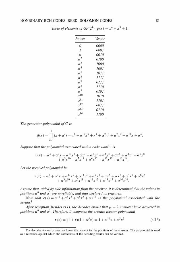
NONBINARY BCH CODES: REED–SOLOMON CODES 81
Table of elements of GF(24), p(x) = x4 + x3 + 1.
Power Vector
0 00001 0001α 0010α2 0100α3 1000α4 1001α5 1011α6 1111α7 0111α8 1110α9 0101α10 1010α11 1101α12 0011α13 0110α14 1100
The generator polynomial of C is
g(x) =6∏
i=1
(x + αi) = x6 + α12x5 + x4 + α2x3 + α7x2 + α11x + α6.
Suppose that the polynomial associated with a code word v is
v(x) = α5 + α3x + α13x2 + αx3 + α7x4 + α4x5 + αx6 + α4x7 + α6x8
+ α3x10 + α5x11 + α6x12 + α13x13 + α10x14.
Let the received polynomial be
r(x) = α7 + α3x + α13x2 + α14x3 + α7x4 + αx5 + αx6 + α4x7 + α6x8
+ α3x10 + α5x11 + α11x12 + α13x13 + α10x14.
Assume that, aided by side information from the receiver, it is determined that the values inpositions α0 and α5 are unreliable, and thus declared as erasures.
Note that e(x) = α14 + α8x3 + α5x5 + αx12 is the polynomial associated with theerrata.1
After reception, besides r(x), the decoder knows that µ = 2 erasures have occurred inpositions α0 and α5. Therefore, it computes the erasure locator polynomial
τ (x) = (1 + x)(1 + α5x) = 1 + α10x + α5x2. (4.16)
1The decoder obviously does not know this, except for the positions of the erasures. This polynomial is usedas a reference against which the correctness of the decoding results can be verified.
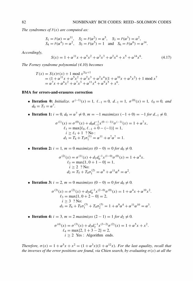
82 NONBINARY BCH CODES: REED–SOLOMON CODES
The syndromes of r(x) are computed as:
S1 = r(α) = α11, S2 = r(α2) = α5, S3 = r(α3) = α2,
S4 = r(α4) = α2, S5 = r(α5) = 1 and S6 = r(α6) = α14.
Accordingly,S(x) = 1 + α11x + α5x2 + α2x3 + α2x4 + x5 + α14x6. (4.17)
The Forney syndrome polynomial (4.10) becomes
T (x) = S(x)τ (x) + 1 mod x2td+1
= (1 + α11x + α5x2 + α2x3 + α2x4)(1 + α10x + α5x2) + 1 mod x7
= α7x + α6x2 + α7x3 + α11x4 + α9x5 + x6.
BMA for errors-and-erasures correction
• Iteration 0: Initialize. σ (−1)(x) = 1, �−1 = 0, d−1 = 1, σ (0)(x) = 1, �0 = 0, andd0 = T3 = α7.
• Iteration 1: i = 0, d0 = α7 �= 0. m = −1 maximizes (−1 + 0) = −1 for d−1 �= 0.
σ (1)(x) = σ (0)(x) + d0d−1−1x(0−(−1))σ (−1)(x) = 1 + α7x,
�1 = max{�0, �−1 + 0 − (−1)} = 1,
i ≥ �1 + 1 ? No :d1 = T4 + T3σ
(1)1 = α11 + α7α7 = 1.
• Iteration 2: i = 1, m = 0 maximizes (0 − 0) = 0 for d0 �= 0.
σ (2)(x) = σ (1)(x) + d1d−10 x(1−0)σ (0)(x) = 1 + α4x.
�2 = max{1, 0 + 1 − 0} = 1,
i ≥ 2 ? No:d2 = T5 + T4σ
(2)1 = α9 + α11α4 = α2.
• Iteration 3: i = 2, m = 0 maximizes (0 − 0) = 0 for d0 �= 0.
σ (3)(x) = σ (2)(x) + d2d−10 x(2−0)σ (0)(x) = 1 + α4x + α10x2.
�3 = max{1, 0 + 2 − 0} = 2,
i ≥ 3 ? No:d3 = T6 + T5σ
(3)1 + T4σ
(3)2 = 1 + α9α4 + α11α10 = α3.
• Iteration 4: i = 3, m = 2 maximizes (2 − 1) = 1 for d2 �= 0.
σ (4)(x) = σ (3)(x) + d3d−12 x(3−2)σ (2)(x) = 1 + α5x + x2.
�4 = max{2, 1 + 3 − 2} = 2,
i ≥ 2 Yes : Algorithm ends.
Therefore, σ(x) = 1 + α5x + x2 = (1 + α3x)(1 + α12x). For the last equality, recall thatthe inverses of the error positions are found, via Chien search, by evaluating σ(x) at all the
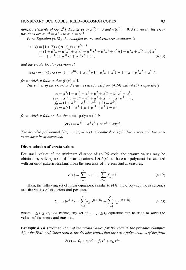
NONBINARY BCH CODES: REED–SOLOMON CODES 83
nonzero elements of GF(24). This gives σ(α12) = 0 and σ(α3) = 0. As a result, the errorpositions are α−12 = α3 and α−3 = α12.
From Equation (4.12), the modified errors-and-erasures evaluator is
ω(x) = [1 + T (x)] σ(x) mod x2td+1
= (1 + α7x + α6x2 + α7x3 + α11x4 + α9x5 + x6)(1 + α5x + x2) mod x7
= 1 + α14x + α11x2 + α11x3 + x4, (4.18)
and the errata locator polynomial
φ(x) = τ (x)σ (x) = (1 + α10x + α5x2)(1 + α5x + x2) = 1 + x + α5x2 + α5x4,
from which it follows that φ′(x) = 1.The values of the errors and erasures are found from (4.14) and (4.15), respectively,
e3 = α3(1 + α11 + α5 + α2 + α3) = α3α5 = α8,
e12 = α12(1 + α2 + α2 + α5 + α12) = α12α4 = α,
f0 = (1 + α14 + α11 + α11 + 1) = α14,
f5 = α5(1 + α9 + α + α11 + α10) = α5,
from which it follows that the errata polynomial is
e(x) = α14 + α8x3 + α5x5 + αx12.
The decoded polynomial v(x) = r(x) + e(x) is identical to v(x). Two errors and two era-sures have been corrected.
Direct solution of errata values
For small values of the minimum distance of an RS code, the erasure values may beobtained by solving a set of linear equations. Let e(x) be the error polynomial associatedwith an error pattern resulting from the presence of ν errors and µ erasures,
e(x) =ν∑
�=1
ej�xj� +
µ∑�′=0
fj ′�xj ′
� . (4.19)
Then, the following set of linear equations, similar to (4.8), hold between the syndromesand the values of the errors and positions:
Si = e(αb+i ) =ν∑
�=1
ej�α(b+i)j� +
µ∑�′=1
fj ′�α(b+i)j ′
� , (4.20)
where 1 ≤ i ≤ 2td . As before, any set of ν + µ ≤ td equations can be used to solve thevalues of the errors and erasures.
Example 4.3.4 Direct solution of the errata values for the code in the previous example:After the BMA and Chien search, the decoder knows that the error polynomial is of the form
e(x) = f0 + e3x3 + f5x
5 + e12x12.
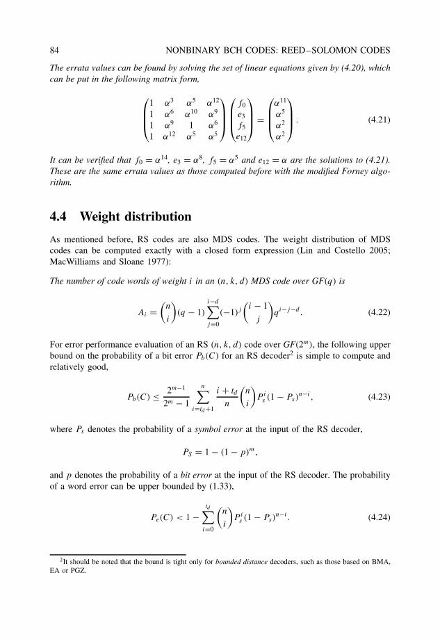
84 NONBINARY BCH CODES: REED–SOLOMON CODES
The errata values can be found by solving the set of linear equations given by (4.20), whichcan be put in the following matrix form,
1 α3 α5 α12
1 α6 α10 α9
1 α9 1 α6
1 α12 α5 α5
f0
e3
f5
e12
=
α11
α5
α2
α2
. (4.21)
It can be verified that f0 = α14, e3 = α8, f5 = α5 and e12 = α are the solutions to (4.21).These are the same errata values as those computed before with the modified Forney algo-rithm.
4.4 Weight distribution
As mentioned before, RS codes are also MDS codes. The weight distribution of MDScodes can be computed exactly with a closed form expression (Lin and Costello 2005;MacWilliams and Sloane 1977):
The number of code words of weight i in an (n, k, d) MDS code over GF(q) is
Ai =(
n
i
)(q − 1)
i−d∑j=0
(−1)j(
i − 1
j
)qi−j−d . (4.22)
For error performance evaluation of an RS (n, k, d) code over GF(2m), the following upperbound on the probability of a bit error Pb(C) for an RS decoder2 is simple to compute andrelatively good,
Pb(C) ≤ 2m−1
2m − 1
n∑i=td+1
i + td
n
(n
i
)P i
s (1 − Ps)n−i , (4.23)
where Ps denotes the probability of a symbol error at the input of the RS decoder,
PS = 1 − (1 − p)m,
and p denotes the probability of a bit error at the input of the RS decoder. The probabilityof a word error can be upper bounded by (1.33),
Pe(C) < 1 −td∑
i=0
(n
i
)P i
s (1 − Ps)n−i . (4.24)
2It should be noted that the bound is tight only for bounded distance decoders, such as those based on BMA,EA or PGZ.
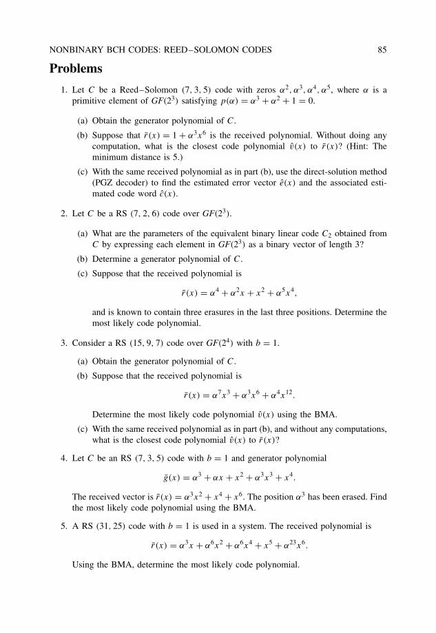
NONBINARY BCH CODES: REED–SOLOMON CODES 85
Problems
1. Let C be a Reed–Solomon (7, 3, 5) code with zeros α2, α3, α4, α5, where α is aprimitive element of GF(23) satisfying p(α) = α3 + α2 + 1 = 0.
(a) Obtain the generator polynomial of C.
(b) Suppose that r(x) = 1 + α3x6 is the received polynomial. Without doing anycomputation, what is the closest code polynomial v(x) to r(x)? (Hint: Theminimum distance is 5.)
(c) With the same received polynomial as in part (b), use the direct-solution method(PGZ decoder) to find the estimated error vector e(x) and the associated esti-mated code word c(x).
2. Let C be a RS (7, 2, 6) code over GF(23).
(a) What are the parameters of the equivalent binary linear code C2 obtained fromC by expressing each element in GF(23) as a binary vector of length 3?
(b) Determine a generator polynomial of C.
(c) Suppose that the received polynomial is
r(x) = α4 + α2x + x2 + α5x4,
and is known to contain three erasures in the last three positions. Determine themost likely code polynomial.
3. Consider a RS (15, 9, 7) code over GF(24) with b = 1.
(a) Obtain the generator polynomial of C.
(b) Suppose that the received polynomial is
r(x) = α7x3 + α3x6 + α4x12.
Determine the most likely code polynomial v(x) using the BMA.
(c) With the same received polynomial as in part (b), and without any computations,what is the closest code polynomial v(x) to r(x)?
4. Let C be an RS (7, 3, 5) code with b = 1 and generator polynomial
g(x) = α3 + αx + x2 + α3x3 + x4.
The received vector is r(x) = α3x2 + x4 + x6. The position α3 has been erased. Findthe most likely code polynomial using the BMA.
5. A RS (31, 25) code with b = 1 is used in a system. The received polynomial is
r(x) = α3x + α6x2 + α6x4 + x5 + α23x6.
Using the BMA, determine the most likely code polynomial.
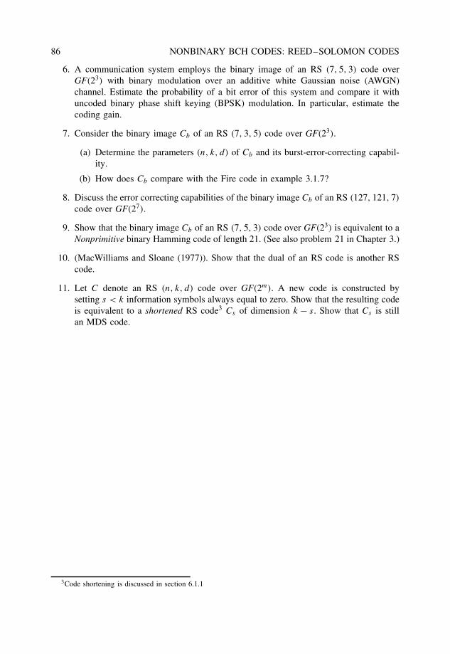
86 NONBINARY BCH CODES: REED–SOLOMON CODES
6. A communication system employs the binary image of an RS (7, 5, 3) code overGF(23) with binary modulation over an additive white Gaussian noise (AWGN)channel. Estimate the probability of a bit error of this system and compare it withuncoded binary phase shift keying (BPSK) modulation. In particular, estimate thecoding gain.
7. Consider the binary image Cb of an RS (7, 3, 5) code over GF(23).
(a) Determine the parameters (n, k, d) of Cb and its burst-error-correcting capabil-ity.
(b) How does Cb compare with the Fire code in example 3.1.7?
8. Discuss the error correcting capabilities of the binary image Cb of an RS (127, 121, 7)
code over GF(27).
9. Show that the binary image Cb of an RS (7, 5, 3) code over GF(23) is equivalent to aNonprimitive binary Hamming code of length 21. (See also problem 21 in Chapter 3.)
10. (MacWilliams and Sloane (1977)). Show that the dual of an RS code is another RScode.
11. Let C denote an RS (n, k, d) code over GF(2m). A new code is constructed bysetting s < k information symbols always equal to zero. Show that the resulting codeis equivalent to a shortened RS code3 Cs of dimension k − s. Show that Cs is stillan MDS code.
3Code shortening is discussed in section 6.1.1
5
Binary convolutional codes
First introduced by Elias (1955), binary convolutional codes are one of the most popularforms of binary error correcting codes that have found numerous applications: wirelesscommunications (IMT-2000, GSM, IS-95), digital terrestrial and satellite communicationand broadcasting systems and space communication systems, just to cite a few. They werereferred to in Elias (1955) as convolutional parity-check symbols codes. Their most populardecoding method to date, the Viterbi algorithm (Viterbi 1967), also finds applications incombinatorially equivalent problems such as maximum likelihood sequence detection (e.g.,equalization) and partial-response signaling (e.g., magnetic recording). Most recently, it hasbeen shown that convolutional codes, when combined with interleaving in a concatenatedscheme, can perform very close to the Shannon limit (Berrou et al. 1993). In this chapter,the basic properties and decoding procedures of binary convolutional codes are described.
5.1 Basic structure
A convolutional code is an error correcting code that processes information serially or,continuously, in short block lengths (Lee 1997). A convolutional encoder has memory, inthe sense that the output symbols depend not only on the input symbols but also on previousinputs and/or outputs. In other words, the encoder is a sequential circuit or a finite-statemachine. The state of the encoder is defined as the contents of the memory. In the computerprograms that implement the Viterbi algorithm and other decoding procedures involving atrellis, found on the ECC web site, a state transition table, indicating the relation betweenthe input, the previous and current state, and the current output, is employed.
A convolutional code consists of the set of all binary sequences produced by a con-volutional encoder. In theory, these sequences have infinite duration. In practice, the stateof the convolutional code is periodically forced to a known state and code sequences areproduced in a block-wise manner.
Example 5.1.1 Consider the convolutional encoder depicted in Figure 5.1. For analysisand decoding purposes, this encoder is described in Table 5.1.
The Art of Error Correcting Coding, Second Edition Robert H. Morelos-Zaragoza 2006 John Wiley & Sons, Ltd. ISBN: 0-470-01558-6
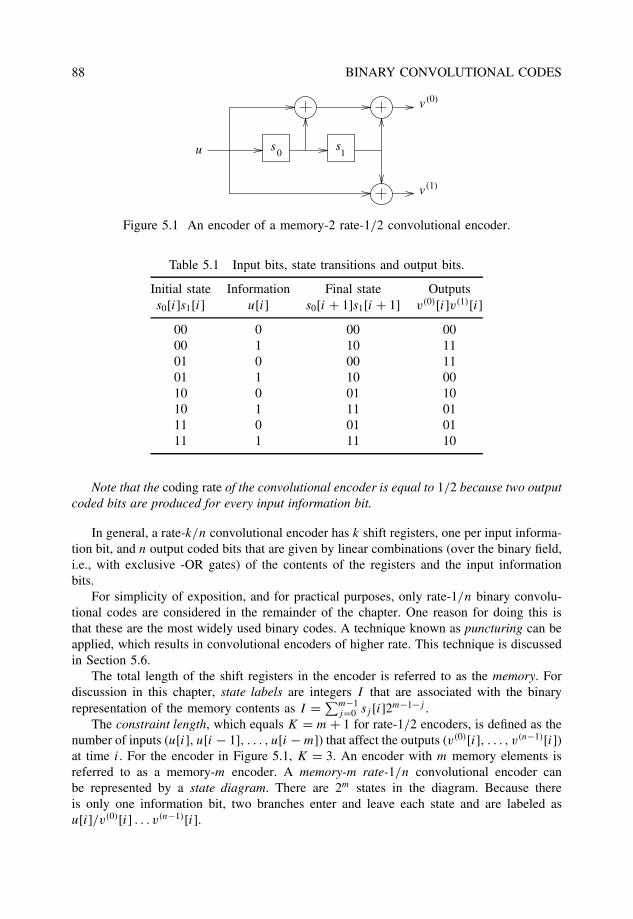
88 BINARY CONVOLUTIONAL CODES
v
v (1)
(0)
u s s0 1
Figure 5.1 An encoder of a memory-2 rate-1/2 convolutional encoder.
Table 5.1 Input bits, state transitions and output bits.
Initial state Information Final state Outputss0[i]s1[i] u[i] s0[i + 1]s1[i + 1] v(0)[i]v(1)[i]
00 0 00 0000 1 10 1101 0 00 1101 1 10 0010 0 01 1010 1 11 0111 0 01 0111 1 11 10
Note that the coding rate of the convolutional encoder is equal to 1/2 because two outputcoded bits are produced for every input information bit.
In general, a rate-k/n convolutional encoder has k shift registers, one per input informa-tion bit, and n output coded bits that are given by linear combinations (over the binary field,i.e., with exclusive -OR gates) of the contents of the registers and the input informationbits.
For simplicity of exposition, and for practical purposes, only rate-1/n binary convolu-tional codes are considered in the remainder of the chapter. One reason for doing this isthat these are the most widely used binary codes. A technique known as puncturing can beapplied, which results in convolutional encoders of higher rate. This technique is discussedin Section 5.6.
The total length of the shift registers in the encoder is referred to as the memory. Fordiscussion in this chapter, state labels are integers I that are associated with the binaryrepresentation of the memory contents as I = ∑m−1
j=0 sj [i]2m−1−j .The constraint length, which equals K = m + 1 for rate-1/2 encoders, is defined as the
number of inputs (u[i], u[i − 1], . . . , u[i − m]) that affect the outputs (v(0)[i], . . . , v(n−1)[i])at time i. For the encoder in Figure 5.1, K = 3. An encoder with m memory elements isreferred to as a memory-m encoder. A memory-m rate-1/n convolutional encoder canbe represented by a state diagram. There are 2m states in the diagram. Because thereis only one information bit, two branches enter and leave each state and are labeled asu[i]/v(0)[i] . . . v(n−1)[i].
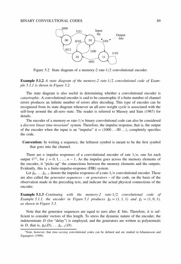
BINARY CONVOLUTIONAL CODES 89
00
01
10
11
0/001/11
0/11 1/00
0/10 1/01
1/10
0/01
Input bit Output
bits
Figure 5.2 State diagram of a memory-2 rate-1/2 convolutional encoder.
Example 5.1.2 A state diagram of the memory-2 rate-1/2 convolutional code of Exam-ple 5.1.1 is shown in Figure 5.2.
The state diagram is also useful in determining whether a convolutional encoder iscatastrophic. A convolutional encoder is said to be catastrophic if a finite number of channelerrors produces an infinite number of errors after decoding. This type of encoder can berecognized from its state diagram whenever an all-zero weight cycle is associated with theself-loop around the all-zero state. The reader is referred to Massey and Sain (1967) fordetails.
The encoder of a memory-m rate-1/n binary convolutional code can also be considereda discrete linear time-invariant1 system. Therefore, the impulse response, that is, the outputof the encoder when the input is an “impulse” u = (1000 . . . 00 . . .), completely specifiesthe code.
Convention: In writing a sequence, the leftmost symbol is meant to be the first symbolthat goes into the channel.
There are n impulse responses of a convolutional encoder of rate 1/n, one for eachoutput v(j), for j = 0, 1, . . . , n − 1. As the impulse goes across the memory elements ofthe encoder, it “picks up” the connections between the memory elements and the outputs.Evidently, this is a finite-impulse-response (FIR) system.
Let g0, . . . gn−1 denote the impulse responses of a rate-1/n convolutional encoder. Theseare also called the generator sequences – or generators – of the code, on the basis of theobservation made in the preceding text, and indicate the actual physical connections of theencoder.
Example 5.1.3 Continuing with the memory-2 rate-1/2 convolutional code ofExample 5.1.1, the encoder in Figure 5.1 produces g0 = (1, 1, 1) and g1 = (1, 0, 1),as shown in Figure 5.3.
Note that the generator sequences are equal to zero after K bits. Therefore, it is suf-ficient to consider vectors of this length. To stress the dynamic nature of the encoder, theindeterminate D (for “delay”) is employed, and the generators are written as polynomialsin D, that is, g0(D), . . . gn−1(D).
1Note, however, that time-varying convolutional codes can be defined and are studied in Johannesson andZigangirov (1999).

90 BINARY CONVOLUTIONAL CODES
0 1u
v
v
1000000...
11100000...
10100000...
(0)
(1)
s s
Figure 5.3 Generator sequences of a memory-2 rate-1/2 convolutional encoder.
Example 5.1.4 For the encoder in Figure 5.1,
g0(D) = 1 + D + D2 and g1(D) = 1 + D2.
In general, when referring to a convolutional code, the generators are expressed as
(g0, . . . , gn−1)
and written in octal form.For the encoder of Example 5.1.4 the generators are (7, 5). The most widely used
convolutional encoder to date is a memory-6 rate-1/2 encoder with generators (171,133).This is the so-called NASA standard code, as it was first used in the Voyager space mis-sions. It is also used in many digital communications standards, as well as in the Control,Communications and Display Subsystem for Satellite (CCSD) standard.
As a result of the dynamical structure of a convolutional encoder, the state diagramcan be represented, as it evolves in time, with a trellis diagram, which is constructed byplacing the state diagram of the code at each time interval, with branches connecting thestates between time i and i + 1, in correspondence with the encoder table. The branchesof the trellis are labeled in the same way as the state diagram.
Convention: When there is no dichotomy, the input information bit does not need toappear explicitly in the branch label. For FIR encoders, the information bit u can beinferred directly from the state transition2:
(s0s1 . . . sm−1) → (us0 . . . sm−2).
It should be emphasized that, in the case of a recursive systematic convolutional(RSC) (infinite-impulse-response (IIR)) encoder, this is not generally the case, as isshown in Section 5.1.1.
Example 5.1.5 For example 5.1.1, the trellis structure is shown in Figure 5.4. Note thatstate transitions (branches) from a state s[i] to a (possibly different) state s ′[i + 1], whichare caused by the input bit u[i] = 0, are the upper branches.
2This simple observation is the basis for using a traceback memory in a Viterbi decoder (VD) to recover theinformation bits from the decoded sequence.
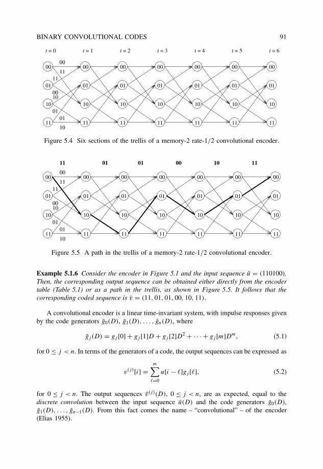
BINARY CONVOLUTIONAL CODES 91
00
01
10
11
00
01
10
11
00
01
10
11
00
01
10
11
00
01
10
11
00
01
10
11
00
01
10
11
11
00
10
01
00
11
10
01
t = 0 t = 1 t = 2 t = 3 t = 4 t = 5 t = 6
Figure 5.4 Six sections of the trellis of a memory-2 rate-1/2 convolutional encoder.
00
01
10
11
11
00
10
01
00
11
10
01
00
01
10
11
00
01
10
11
00
01
10
11
00
01
10
11
00
01
10
11
00
01
10
11
11 01 00 10 1101
Figure 5.5 A path in the trellis of a memory-2 rate-1/2 convolutional encoder.
Example 5.1.6 Consider the encoder in Figure 5.1 and the input sequence u = (110100).Then, the corresponding output sequence can be obtained either directly from the encodertable (Table 5.1) or as a path in the trellis, as shown in Figure 5.5. It follows that thecorresponding coded sequence is v = (11, 01, 01, 00, 10, 11).
A convolutional encoder is a linear time-invariant system, with impulse responses givenby the code generators g0(D), g1(D), . . . , gn(D), where
gj (D) = gj [0] + gj [1]D + gj [2]D2 + · · · + gj [m]Dm, (5.1)
for 0 ≤ j < n. In terms of the generators of a code, the output sequences can be expressed as
v(j)[i] =m∑
�=0
u[i − �]gj [�], (5.2)
for 0 ≤ j < n. The output sequences v(j)(D), 0 ≤ j < n, are as expected, equal to thediscrete convolution between the input sequence u(D) and the code generators g0(D),g1(D), . . . , gn−1(D). From this fact comes the name – “convolutional” – of the encoder(Elias 1955).
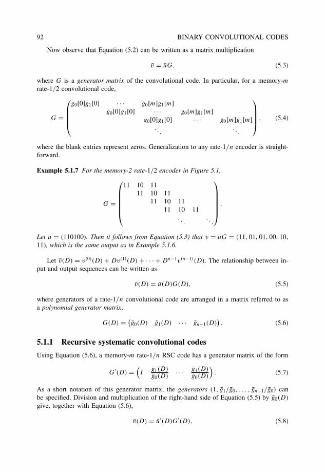
92 BINARY CONVOLUTIONAL CODES
Now observe that Equation (5.2) can be written as a matrix multiplication
v = uG, (5.3)
where G is a generator matrix of the convolutional code. In particular, for a memory-mrate-1/2 convolutional code,
G =
g0[0]g1[0] · · · g0[m]g1[m]g0[0]g1[0] · · · g0[m]g1[m]
g0[0]g1[0] · · · g0[m]g1[m]. . .
. . .
, (5.4)
where the blank entries represent zeros. Generalization to any rate-1/n encoder is straight-forward.
Example 5.1.7 For the memory-2 rate-1/2 encoder in Figure 5.1,
G =
11 10 1111 10 11
11 10 1111 10 11
. . .. . .
.
Let u = (110100). Then it follows from Equation (5.3) that v = uG = (11, 01, 01, 00, 10,
11), which is the same output as in Example 5.1.6.
Let v(D) = v(0)(D) + Dv(1)(D) + · · · + Dn−1v(n−1)(D). The relationship between in-put and output sequences can be written as
v(D) = u(D)G(D), (5.5)
where generators of a rate-1/n convolutional code are arranged in a matrix referred to asa polynomial generator matrix,
G(D) = (g0(D) g1(D) · · · gn−1(D)
). (5.6)
5.1.1 Recursive systematic convolutional codes
Using Equation (5.6), a memory-m rate-1/n RSC code has a generator matrix of the form
G′(D) =(I
g1(D)g0(D)
· · · g1(D)g0(D)
). (5.7)
As a short notation of this generator matrix, the generators (1, g1/g0, . . . , gn−1/g0) canbe specified. Division and multiplication of the right-hand side of Equation (5.5) by g0(D)
give, together with Equation (5.6),
v(D) = u′(D)G′(D), (5.8)
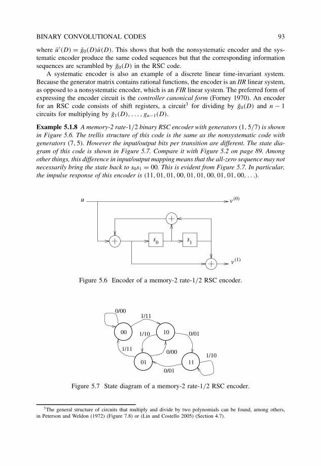
BINARY CONVOLUTIONAL CODES 93
where u′(D) = g0(D)u(D). This shows that both the nonsystematic encoder and the sys-tematic encoder produce the same coded sequences but that the corresponding informationsequences are scrambled by g0(D) in the RSC code.
A systematic encoder is also an example of a discrete linear time-invariant system.Because the generator matrix contains rational functions, the encoder is an IIR linear system,as opposed to a nonsystematic encoder, which is an FIR linear system. The preferred form ofexpressing the encoder circuit is the controller canonical form (Forney 1970). An encoderfor an RSC code consists of shift registers, a circuit3 for dividing by g0(D) and n − 1circuits for multiplying by g1(D), . . . , gn−1(D).
Example 5.1.8 A memory-2 rate-1/2 binary RSC encoder with generators (1, 5/7) is shownin Figure 5.6. The trellis structure of this code is the same as the nonsystematic code withgenerators (7, 5). However the input/output bits per transition are different. The state dia-gram of this code is shown in Figure 5.7. Compare it with Figure 5.2 on page 89. Amongother things, this difference in input/output mapping means that the all-zero sequence may notnecessarily bring the state back to s0s1 = 00. This is evident from Figure 5.7. In particular,the impulse response of this encoder is (11, 01, 01, 00, 01, 01, 00, 01, 01, 00, . . .).
0
v (1)
vu (0)
s s1
Figure 5.6 Encoder of a memory-2 rate-1/2 RSC encoder.
00
01
10
11
0/00
1/11
1/10 0/01
1/10
0/01
0/00
1/11
Figure 5.7 State diagram of a memory-2 rate-1/2 RSC encoder.
3The general structure of circuits that multiply and divide by two polynomials can be found, among others,in Peterson and Weldon (1972) (Figure 7.8) or (Lin and Costello 2005) (Section 4.7).
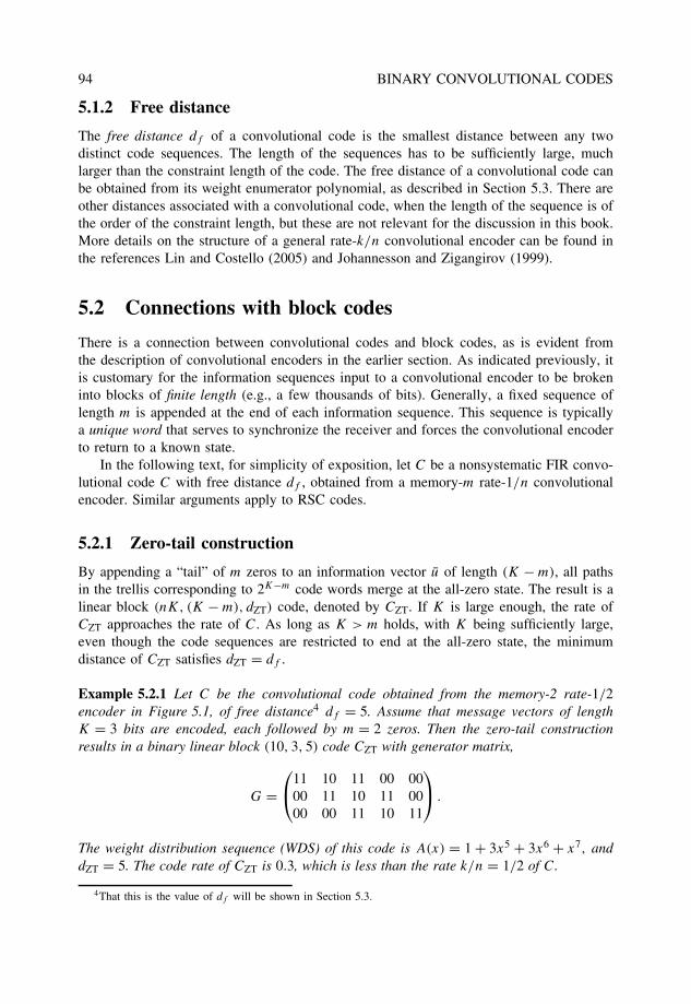
94 BINARY CONVOLUTIONAL CODES
5.1.2 Free distance
The free distance df of a convolutional code is the smallest distance between any twodistinct code sequences. The length of the sequences has to be sufficiently large, muchlarger than the constraint length of the code. The free distance of a convolutional code canbe obtained from its weight enumerator polynomial, as described in Section 5.3. There areother distances associated with a convolutional code, when the length of the sequence is ofthe order of the constraint length, but these are not relevant for the discussion in this book.More details on the structure of a general rate-k/n convolutional encoder can be found inthe references Lin and Costello (2005) and Johannesson and Zigangirov (1999).
5.2 Connections with block codes
There is a connection between convolutional codes and block codes, as is evident fromthe description of convolutional encoders in the earlier section. As indicated previously, itis customary for the information sequences input to a convolutional encoder to be brokeninto blocks of finite length (e.g., a few thousands of bits). Generally, a fixed sequence oflength m is appended at the end of each information sequence. This sequence is typicallya unique word that serves to synchronize the receiver and forces the convolutional encoderto return to a known state.
In the following text, for simplicity of exposition, let C be a nonsystematic FIR convo-lutional code C with free distance df , obtained from a memory-m rate-1/n convolutionalencoder. Similar arguments apply to RSC codes.
5.2.1 Zero-tail construction
By appending a “tail” of m zeros to an information vector u of length (K − m), all pathsin the trellis corresponding to 2K−m code words merge at the all-zero state. The result is alinear block (nK, (K − m), dZT) code, denoted by CZT. If K is large enough, the rate ofCZT approaches the rate of C. As long as K > m holds, with K being sufficiently large,even though the code sequences are restricted to end at the all-zero state, the minimumdistance of CZT satisfies dZT = df .
Example 5.2.1 Let C be the convolutional code obtained from the memory-2 rate-1/2encoder in Figure 5.1, of free distance4 df = 5. Assume that message vectors of lengthK = 3 bits are encoded, each followed by m = 2 zeros. Then the zero-tail constructionresults in a binary linear block (10, 3, 5) code CZT with generator matrix,
G =11 10 11 00 00
00 11 10 11 0000 00 11 10 11
.
The weight distribution sequence (WDS) of this code is A(x) = 1 + 3x5 + 3x6 + x7, anddZT = 5. The code rate of CZT is 0.3, which is less than the rate k/n = 1/2 of C.
4That this is the value of df will be shown in Section 5.3.
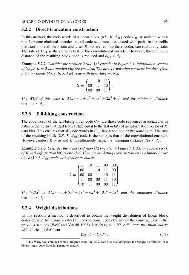
BINARY CONVOLUTIONAL CODES 95
5.2.2 Direct-truncation construction
In this method, the code words of a linear block (nK, K, dDT) code CDT associated with arate-k/n convolutional encoder are all code sequences associated with paths in the trellisthat start in the all-zero state and, after K bits are fed into the encoder, can end at any state.The rate of CDT is the same as that of the convolutional encoder. However, the minimumdistance of the resulting block code is reduced and dDT < df .
Example 5.2.2 Consider the memory-2 rate-1/2 encoder in Figure 5.1. Information vectorsof length K = 3 information bits are encoded. The direct truncation construction then givesa binary linear block (6, 3, dDT) code with generator matrix,
G =11 10 11
00 11 1000 00 11
.
The WDS of this code is A(x) = 1 + x2 + 3x3 + 2x4 + x5 and the minimum distancedDT = 2 < df .
5.2.3 Tail-biting construction
The code words of the tail-biting block code CTB are those code sequences associated withpaths in the trellis that start from a state equal to the last m bits of an information vector of K
data bits. This ensures that all code words in CTB begin and end at the same state. The rateof the resulting block (2K, K, dTB) code is the same as that of the convolutional encoder.However, unless K > m and K is sufficiently large, the minimum distance dTB ≤ df .
Example 5.2.3 Consider the memory-2 rate-1/2 encoder in Figure 5.1. Assume that a blockof K = 5 information bits is encoded. Then the tail-biting construction gives a binary linearblock (10, 5, dTB) code with generator matrix,
G =
11 10 11 00 0000 11 10 11 0000 00 11 10 1111 00 00 11 1010 11 00 00 11
.
The WDS5 is A(x) = 1 + 5x3 + 5x4 + 6x5 + 10x6 + 5x7 and the minimum distancedTB = 3 < df .
5.2.4 Weight distributions
In this section, a method is described to obtain the weight distribution of linear blockcodes derived from binary rate-1/n convolutional codes by any of the constructions in theprevious sections (Wolf and Viterbi 1996). Let �(x) be a 2m × 2m state transition matrixwith entries of the form
�ij (x) = δij xhij , (5.9)
5This WDS was obtained with a program from the ECC web site that computes the weight distribution of abinary linear code from its generator matrix.
96 BINARY CONVOLUTIONAL CODES
where δij = 1, if and only if there is a transition from state i to state j , and δij = 0otherwise, and hij is the Hamming weight of the corresponding output vector (of length n).
Example 5.2.4 For the convolutional encoder with the state diagram shown in Figure 5.2,the state transition matrix �(x) is given by
�(x) =
1 0 x2 0x2 0 1 00 x 0 x
0 x 0 x
.
The WDS of a binary linear block (n, k) code constructed from any of the previous methodscan be obtained by symbolically raising matrix �(x) to the �-th power, denoted by ��(x),and combining different terms.
The term ��ij (x) gives the weight distribution of trellis paths that start in state i and
end in state j after � time intervals. For the ZT construction, the value � = k + m is used,while for both DT and TB constructions, � = k. The WDSs for each of the constructionmethods presented in the preceding text can be computed as follows.
• ZT construction:
A(x) = �k+m00 (x).
• DT construction:
A(x) =2m∑j=0
�k0j (x).
• TB construction:
A(x) =2m∑j=0
�kjj (x).
Example 5.2.5 Consider again the memory-2 rate-1/2 convolutional encoder. Then
�3(x) =
1 + x5 x3 + x4 x2 + x3 x3 + x4
x2 + x3 x5 + x2 x4 + x x5 + x2
x3 + x4 x2 + x3 x5 + x2 x2 + x3
x3 + x4 x2 + x3 x5 + x2 x2 + x3
.
The WDS of the code from the DT construction in Example 5.2.2 is obtained by adding theterms in the first row of �3(x).
References on other methods of computing the WDS of a linear block code derivedfrom a convolutional code are Fossorier et al. (1999), Chaudhari and Khandani (2001) andDesaki et al. (1994).
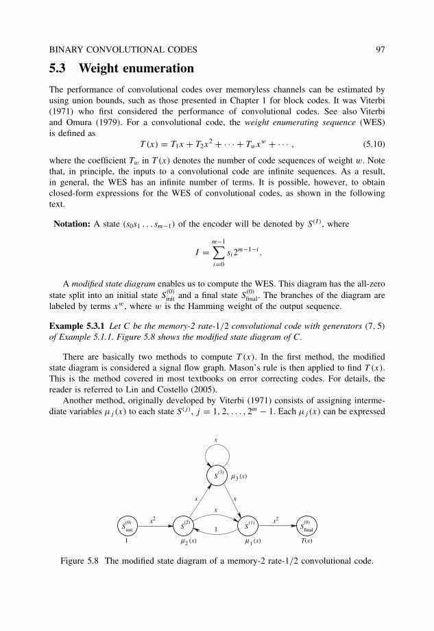
BINARY CONVOLUTIONAL CODES 97
5.3 Weight enumeration
The performance of convolutional codes over memoryless channels can be estimated byusing union bounds, such as those presented in Chapter 1 for block codes. It was Viterbi(1971) who first considered the performance of convolutional codes. See also Viterbiand Omura (1979). For a convolutional code, the weight enumerating sequence (WES)is defined as
T (x) = T1x + T2x2 + · · · + Twxw + · · · , (5.10)
where the coefficient Tw in T (x) denotes the number of code sequences of weight w. Notethat, in principle, the inputs to a convolutional code are infinite sequences. As a result,in general, the WES has an infinite number of terms. It is possible, however, to obtainclosed-form expressions for the WES of convolutional codes, as shown in the followingtext.
Notation: A state (s0s1 . . . sm−1) of the encoder will be denoted by S(I), where
I =m−1∑i=0
si2m−1−i .
A modified state diagram enables us to compute the WES. This diagram has the all-zerostate split into an initial state S
(0)init and a final state S
(0)final. The branches of the diagram are
labeled by terms xw , where w is the Hamming weight of the output sequence.
Example 5.3.1 Let C be the memory-2 rate-1/2 convolutional code with generators (7, 5)
of Example 5.1.1. Figure 5.8 shows the modified state diagram of C.
There are basically two methods to compute T (x). In the first method, the modifiedstate diagram is considered a signal flow graph. Mason’s rule is then applied to find T (x).This is the method covered in most textbooks on error correcting codes. For details, thereader is referred to Lin and Costello (2005).
Another method, originally developed by Viterbi (1971) consists of assigning interme-diate variables µj (x) to each state S(j), j = 1, 2, . . . , 2m − 1. Each µj(x) can be expressed
x2 x2
x x
x
1
x
S
S S
µ µ
µ
T(x)
S
1
init
(0) (2) (1)
(3)3
1
Sfinal
(0)
(x)
(x)
(x)2
Figure 5.8 The modified state diagram of a memory-2 rate-1/2 convolutional code.
98 BINARY CONVOLUTIONAL CODES
as a linear combination of weighted variables associated with states connected to S(j),
µj(x) =2m−1∑k=1k �=j
µk(x)δkj xhkj , (5.11)
for all k ∈ {1, 2, . . . , 2m − 1}, k �= j , and where δij and hkj are defined as in Equation (5.9).The initial state S
(0)init is assigned a variable of value 1, while WES T (x) is assigned as a
variable to the final state S(0)final.
This yields a system of linear equations that can be solved to find µ1(x), from which,using the adopted notation to designate states,
T (x) = µ1(x)xh10 . (5.12)
Example 5.3.2 Consider the modified state diagram in Figure 5.8. The following set ofequations is obtained
µ1(x) = µ2(x)x + µ3(x)x
µ2(x) = x2 + µ1(x)
µ3(x) = µ2(x)x + µ3(x)x (5.13)
and T (x) = µ1(x)x2. Equations (5.13) can be written in matrix form as 1 −x −x
−1 1 00 −x 1 − x
µ1(x)
µ2(x)
µ3(x)
=
0
x2
0
, (5.14)
and solving for µ1(x) gives
µ1(x) = x3
1 − 2x.
It follows that
T (x) = x5
1 − 2x= x5 + 2x6 + 4x7 + 8x8 + · · · (5.15)
This shows that the minimum free distance is df = 5 for the binary 4-state rate-1/2 convo-lutional code with generators (7, 5).
More detailed information about the structure of a convolutional code is obtained bylabeling the modified state diagram with terms of the form xwy�zm, where w is the Hammingweight of the coded outputs, � is the Hamming weight of the input vector (of length equalto k, in general, for a rate-k/n convolutional code) and m is the number of branchesdiffering from the all-zero sequence. (See Lin and Costello (2005), p. 493.) This resultsin a complete weight enumerator sequence (CWES), T (x, y, z), which can be used toderive various bounds on the error performance of convolutional codes (Johannesson andZigangirov 1999; Lin and Costello 2005; Viterbi 1971). A WES similar to the CWES wasused to estimate the performance of turbo codes in Benedetto and Montorsi (1996).

BINARY CONVOLUTIONAL CODES 99
x2 x2
xz
xz
x
S
S S
µ µ
µ
T(x)
S
1
init
(0) (2) (1)
(3)3
2
Sfinal
(0)
(x)
(x)
(x)
yzyz
z
xyz
yz
1
Figure 5.9 The modified state diagram of a memory-2 rate-1/2 convolutional code.
Example 5.3.3 Continuing with Example 5.3.2 , a modified state diagram for the computa-tion of the CWES is shown in Figure 5.9.
The equations are 1 −xz −xz
−yz 1 00 −xyz 1 − xyz
µ1(x)
µ2(x)
µ3(x)
=
0
x2yz
0
,
with T (x, y, z) = x2zµ1(x). The solution is:
T (x, y, z) = x5yz3
1 − xyz(1 + z)= x5yz3 + x6y2z4(1 + z) + x7y3z5(1 + z)2 + · · ·
5.4 Performance bounds
Bounds on the bit error probability of a binary convolutional code of rate k/n can beobtained with the aid of the CWES described in the previous section. For transmission overa binary symmetric channel (BSC) and binary transmission over an additive white Gaus-sian noise (AWGN) channel (Viterbi and Omura 1979) and maximum-likelihood decoding(MLD)6, the following upper bounds hold, respectively,
Pb <1
k
∂T (x, y, z)
∂y
∣∣∣∣x=√
4p(1−p),y=1,z=1, (5.16)
Pb <1
k
∂T (x, y, z)
∂y
∣∣∣∣x=e−REb/N0 ,y=1,z=1
, (5.17)
where the energy-per-bit-to-noise ratio Eb/N0 is related to the energy-per-symbol-to-noiseratio Es/N0 via the code rate R = k/n is as follows:
Eb
N0= 1
R
Es
N0. (5.18)
6An example of an MLD algorithm is the Viterbi decoder, explained in the next section.
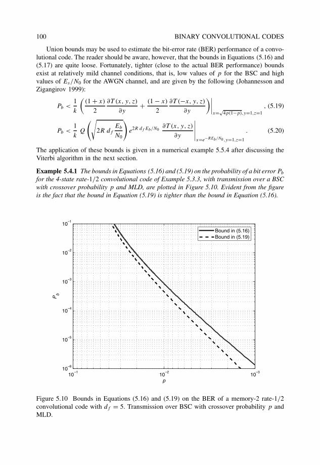
100 BINARY CONVOLUTIONAL CODES
Union bounds may be used to estimate the bit-error rate (BER) performance of a convo-lutional code. The reader should be aware, however, that the bounds in Equations (5.16) and(5.17) are quite loose. Fortunately, tighter (close to the actual BER performance) boundsexist at relatively mild channel conditions, that is, low values of p for the BSC and highvalues of Es/N0 for the AWGN channel, and are given by the following (Johannesson andZigangirov 1999):
Pb <1
k
((1 + x)
2
∂T (x, y, z)
∂y+ (1 − x)
2
∂T (−x, y, z)
∂y
)∣∣∣∣x=√
4p(1−p),y=1,z=1, (5.19)
Pb <1
kQ
(√2R df
Eb
N0
)e2R df Eb/N0
∂T (x, y, z)
∂y
∣∣∣∣∣x=e−REb/N0 ,y=1,z=1
. (5.20)
The application of these bounds is given in a numerical example 5.5.4 after discussing theViterbi algorithm in the next section.
Example 5.4.1 The bounds in Equations (5.16) and (5.19) on the probability of a bit error Pb
for the 4-state rate-1/2 convolutional code of Example 5.3.3, with transmission over a BSCwith crossover probability p and MLD, are plotted in Figure 5.10. Evident from the figureis the fact that the bound in Equation (5.19) is tighter than the bound in Equation (5.16).
10–3
10–2
10–1
10–6
10–5
10–4
10–3
10–2
10–1
p
Pb
Bound in (5.16)Bound in (5.19)
Figure 5.10 Bounds in Equations (5.16) and (5.19) on the BER of a memory-2 rate-1/2convolutional code with df = 5. Transmission over BSC with crossover probability p andMLD.
BINARY CONVOLUTIONAL CODES 101
5.5 Decoding: Viterbi algorithm with Hamming metrics
The trellis of convolutional codes has a regular structure. It is possible to take advantageof the repetitive pattern of the trellis in decoding. However, for linear block codes obtainedfrom terminating convolutional codes and long information sequences, MLD is simply toocomplex and inefficient to implement.
An efficient solution to the decoding problem is a dynamic programming algorithmknown as the Viterbi algorithm, also known as the Viterbi decoder (VD). This is a maximumlikelihood decoder in the sense that it finds the closest coded sequence v to the receivedsequence r by processing the sequences on an information bit-by-bit (branches of the trellis)basis. In other words, instead of keeping a score of each possible coded sequence, the VDtracks the states of the trellis.
5.5.1 Maximum-likelihood decoding and metrics
The likelihood of a received sequence R after transmission over a noisy memoryless channel,given that a coded sequence V is sent, is defined as the conditional probability densityfunction
pR|V (r|v) =n−1∏i=0
P (ri |vi), (5.21)
where V and R are the transmitted and received sequences, respectively.It is easy to show that for a BSC with parameter p,
pR|V (r|v) =n−1∏i=0
(1 − p)
(p
1 − p
)dH (ri ,vi )
, (5.22)
with dH (ri, vi) = 1, if ri �= vi , and dH (ri, vi) = 0, if ri = vi . That is, dH (ri, vi) is theHamming distance between bits ri and vi . For an AWGN channel, the likelihood is given by
pR|V (r|v) =n−1∏i=0
1√πN0
e− 1
N0(ri−m(vi ))
2
, (5.23)
where m(·) denotes a binary modulated signal. Here, m is defined as a one-to-one mappingbetween bits {0, 1} and real numbers {−√
Es, +√Es}, where Es is the energy per symbol.
This mapping is also known as binary phase-shift keying (BPSK) modulation or polarmapping.
An MLD selects a coded sequence v′ that maximizes Equation (5.21). By taking the log-arithm of Equation (5.21), the following can be shown. For the BSC, an MLD is equivalentto choosing the code sequence that minimizes the Hamming distance
dH (r, v) =n−1∑i=0
dH (ri, vi). (5.24)
Similarly, for the AWGN channel, it is the squared Euclidean distance
dE(r, v) =n−1∑i=0
(r − ¯m(v)
)2(5.25)
102 BINARY CONVOLUTIONAL CODES
that is minimized by the coded sequence selected by the MLD. In this section, a BSC withcrossover error probability p is considered. The AWGN channel is covered in Chapter 7.
5.5.2 The Viterbi algorithm
Let S(k)i denote a state in the trellis at stage i. Each state S
(k)i in the trellis is assigned a
state metric, or simply a metric, M(S(k)i ), and a path in the trellis, y(k). A key observation
in applying the Viterbi algorithm is:
With i being the time, most likely paths per state y(k)i (the ones closest to the
received sequence) will eventually coincide at some time i − �.
In his paper, Viterbi (1967) indicates that the value of � for memory-m rate-1/2 binaryconvolutional codes should be � > 5m. The VD operates within a range of L receivedn-tuples (output bits per state transition) known as the decoding depth. The value of L
must be such that L > �.In the following text, the Viterbi algorithm applied to a memory-m rate-1/n binary
convolutional code is described and its operation illustrated via a simple example. Someadditional notation is needed: Let
v[i] = (v0[i]v1[i] . . . vn−1[i])
denote the coded bits in a branch (state transition), and let
r[i] = (r0[i]r1[i] . . . rn−1[i])
denote the output of the channel.
Basic decoding steps
Initialization
Set i = 0. Set metrics and paths
M(S(k)0 ) = 0, y
(k)0 = () (empty).
The specific way in which the initialization of the paths is performed is irrelevant,as shown later. For the sake of clarity of presentation of the algorithm, it is assumedthat the paths are represented as lists that are initialized to the empty list.
1. Branch metric computation
At stage i, compute the partial branch metrics
BM(b)i = dH (r[i], v[i]), (5.26)
b�= ∑n−1
�=0 v�[i]2n−1−�, associated with the n outputs v[i] of every branch (or statetransition) and the n received bits r[i].
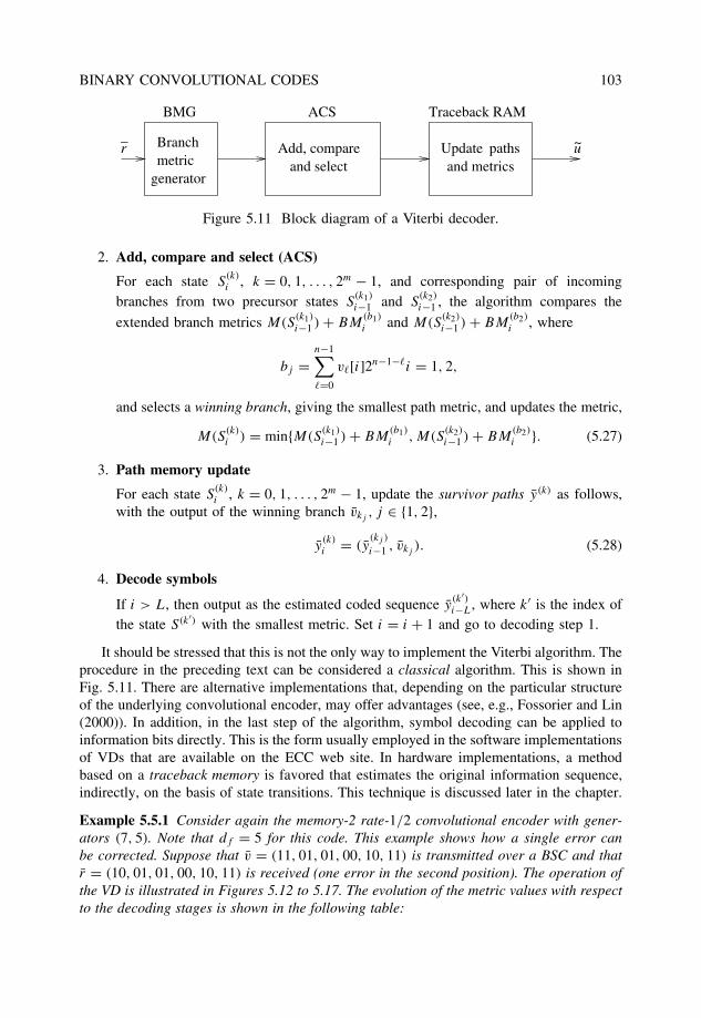
BINARY CONVOLUTIONAL CODES 103
Branchmetric
generator
Add, compareand select
Update pathsand metrics
r_
u~
BMG ACS Traceback RAM
Figure 5.11 Block diagram of a Viterbi decoder.
2. Add, compare and select (ACS)
For each state S(k)i , k = 0, 1, . . . , 2m − 1, and corresponding pair of incoming
branches from two precursor states S(k1)
i−1 and S(k2)
i−1 , the algorithm compares the
extended branch metrics M(S(k1)
i−1 ) + BM(b1)
i and M(S(k2)
i−1 ) + BM(b2)
i , where
bj =n−1∑�=0
v�[i]2n−1−�i = 1, 2,
and selects a winning branch, giving the smallest path metric, and updates the metric,
M(S(k)i ) = min{M(S
(k1)
i−1 ) + BM(b1)i , M(S
(k2)
i−1 ) + BM(b2)i }. (5.27)
3. Path memory update
For each state S(k)i , k = 0, 1, . . . , 2m − 1, update the survivor paths y(k) as follows,
with the output of the winning branch vkj, j ∈ {1, 2},
y(k)i = (y
(kj )
i−1 , vkj). (5.28)
4. Decode symbols
If i > L, then output as the estimated coded sequence y(k′)i−L, where k′ is the index of
the state S(k′) with the smallest metric. Set i = i + 1 and go to decoding step 1.
It should be stressed that this is not the only way to implement the Viterbi algorithm. Theprocedure in the preceding text can be considered a classical algorithm. This is shown inFig. 5.11. There are alternative implementations that, depending on the particular structureof the underlying convolutional encoder, may offer advantages (see, e.g., Fossorier and Lin(2000)). In addition, in the last step of the algorithm, symbol decoding can be applied toinformation bits directly. This is the form usually employed in the software implementationsof VDs that are available on the ECC web site. In hardware implementations, a methodbased on a traceback memory is favored that estimates the original information sequence,indirectly, on the basis of state transitions. This technique is discussed later in the chapter.
Example 5.5.1 Consider again the memory-2 rate-1/2 convolutional encoder with gener-ators (7, 5). Note that df = 5 for this code. This example shows how a single error canbe corrected. Suppose that v = (11, 01, 01, 00, 10, 11) is transmitted over a BSC and thatr = (10, 01, 01, 00, 10, 11) is received (one error in the second position). The operation ofthe VD is illustrated in Figures 5.12 to 5.17. The evolution of the metric values with respectto the decoding stages is shown in the following table:
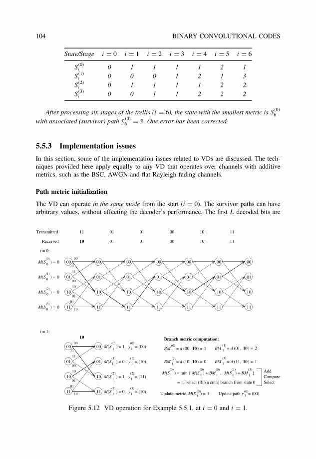
104 BINARY CONVOLUTIONAL CODES
State/Stage i = 0 i = 1 i = 2 i = 3 i = 4 i = 5 i = 6
S(0)i 0 1 1 1 1 2 1
S(1)i 0 0 0 1 2 1 3
S(2)i 0 1 1 1 1 2 2
S(3)i 0 0 1 1 2 2 2
After processing six stages of the trellis (i = 6), the state with the smallest metric is S(0)6
with associated (survivor) path y(0)6 = v. One error has been corrected.
5.5.3 Implementation issues
In this section, some of the implementation issues related to VDs are discussed. The tech-niques provided here apply equally to any VD that operates over channels with additivemetrics, such as the BSC, AWGN and flat Rayleigh fading channels.
Path metric initialization
The VD can operate in the same mode from the start (i = 0). The survivor paths can havearbitrary values, without affecting the decoder’s performance. The first L decoded bits are
00
01
10
11
11
01
AddCompareSelect
Transmitted
Received 01 00 10 11
00 10 1101
0110
t = 0:
00
01
10
11
00
01
10
11
00
01
10
11
00
01
10
11
00
01
10
11
M(S ) = 00
M(S ) = 0
M(S ) = 0
00
01
10
11
00
11
00
10
01
10
M(S ) = 00
0
0
00
01
10
11
00
11
11
00
10
01
01
10
00
01
10
11
10
(0)
(1)
(2)
(3)
t = 1:
Branch metric computation:
1 10(0)
BM = d (00, ) = 11 10
1 10 1 10
(1)
(2) (3)
(0)
1M(S ) = min { M(S ) + BM , M(S ) + BM }0 0
(0) (1)(0) (3)
1 1
Update metric M(S ) = 1(0)1 1
(0)
1
(0) (0)
1M(S ) = 1,
1 1
1 1M(S ) = 1,
1 1
(1)M(S ) = 0, y = (10)
(1)
(2) (2)
(3) (3)M(S ) = 0, y = (10)
= 1, select (flip a coin) branch from state 0
Update path y = (00)
y = (00)
y = (11)
11 01
BM = d (01, ) = 2
BM = d (11, ) = 1BM = d (10, ) = 0
Figure 5.12 VD operation for Example 5.5.1, at i = 0 and i = 1.
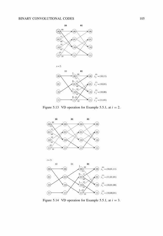
BINARY CONVOLUTIONAL CODES 105
00
11
11
00
10
01
01
10
(0)
(1)
(2)
(3)
2
2
2
2
y = (10,11)
y = (10,01)
y = (10,00)
y = (11,01)
10 01
00
01
10
11
00
11
00
10
01
10
00
01
10
11
00
01
10
11
10
00
01
10
11
1
0
1
0
t = 2:
00
01
10
11
00
01
10
11
11
01
01
Figure 5.13 VD operation for Example 5.5.1, at i = 2.
00
01
10
11
11
01
00
11
11
00
10
01
01
10
(0)
(1)
(2)
(3)y = (10,00,01)
3
3
3
3
y = (10,01,11)
y = (11,01,01)
y = (10,01,00)
00
01
10
11
00
11
00
10
01
10
00
01
10
11
10
00
01
10
11
01
00
01
10
11
1
0
1
1
01
00
01
10
11
t = 3:
00
01
10
11
00
01
10
11
0110 01
Figure 5.14 VD operation for Example 5.5.1, at i = 3.
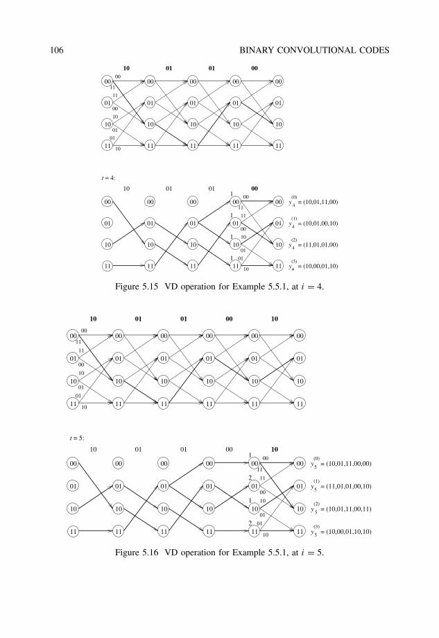
106 BINARY CONVOLUTIONAL CODES
00
01
10
11
11
01
(0)
(1)
(2)
(3)
4
4
4
4y = (10,00,01,10)
y = (10,01,11,00)
y = (10,01,00,10)
y = (11,01,01,00)
00
01
10
11
00
11
00
10
01
10
00
01
10
11
10
00
01
10
11
00
01
10
11
00
01
10
11
001
1
1
1
00
01
10
11
01 0010 01
00
01
10
11
00
01
10
11
00
01
10
11
00
11
11
00
10
01
01
10
01 01
t = 4:
Figure 5.15 VD operation for Example 5.5.1, at i = 4.
(0)
(1)
(2)
(3)
5
5
5
5y = (10,00,01,10,10)
y = (10,01,11,00,00)
y = (11,01,01,00,10)
y = (10,01,11,00,11)
00
01
10
11
00
11
00
10
01
10
00
01
10
11
10
00
01
10
11
01
00
01
10
11
01
00
01
10
11
00
00
01
10
11
00
01
10
11
1
2
1
2
10
t = 5:
01 00 1010 01
00
01
10
11
11
01
00
01
10
11
00
01
10
11
00
01
10
11
00
01
10
11
00
11
11
00
10
01
01
10
Figure 5.16 VD operation for Example 5.5.1, at i = 5.
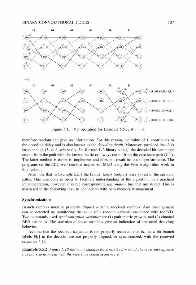
BINARY CONVOLUTIONAL CODES 107
00
01
10
11
00
11
00
10
01
10
00
01
10
11
10
00
01
10
11
01
00
01
10
11
01
00
01
10
11
00
00
01
10
11
00
01
10
11
102
1
2
2
11
00
01
10
11
t = 6:
00
11
11
00
10
01
01
10
(0)
(1)
(2)
(3)
6
6
6
6y = (10,00,01,10,10,10)
y = (11,01,01,00,10,11)
y = (10,00,01,10,10,01)
y = (10,01,11,00,00,11)
00
01
10
11
00
01
10
11
00
01
10
11
00
01
10
11
00
01
10
11
00
01
10
11
11
01
01 00 10 1110 01
Figure 5.17 VD operation for Example 5.5.1, at i = 6.
therefore random and give no information. For this reason, the value of L contributes tothe decoding delay and is also known as the decoding depth. Moreover, provided that L islarge enough (L � �, where � > 5m for rate-1/2 binary codes), the decoded bit can eitheroutput from the path with the lowest metric or always output from the zero state path (y(0)).The latter method is easier to implement and does not result in loss of performance. Theprograms on the ECC web site that implement MLD using the Viterbi algorithm work inthis fashion.
Also note that in Example 5.5.1 the branch labels (output) were stored in the survivorpaths. This was done in order to facilitate understanding of the algorithm. In a practicalimplementation, however, it is the corresponding information bits that are stored. This isdiscussed in the following text, in connection with path memory management.
Synchronization
Branch symbols must be properly aligned with the received symbols. Any misalignmentcan be detected by monitoring the value of a random variable associated with the VD.Two commonly used synchronization variables are (1) path metric growth, and (2) channelBER estimates. The statistics of these variables give an indication of abnormal decodingbehavior.
Assume that the received sequence is not properly received, that is, the n-bit branchlabels v[i] in the decoder are not properly aligned, or synchronized, with the receivedsequence r[i].
Example 5.5.2 Figure 5.18 shows an example for a rate-1/2 in which the received sequencer is not synchronized with the reference coded sequence v.
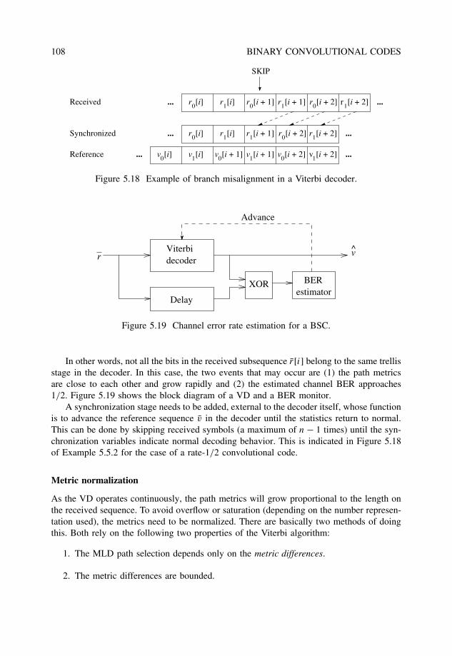
108 BINARY CONVOLUTIONAL CODES
r0[i] r1[i] r0[i + 1] r1[i + 1] r0[i + 2] 1[i + 2]r
v0[i] v1[i] v0[i + 1] v1[i + 1] v0[i + 2] 1[i + 2]v
r0[i] r1[i] r1[i + 1] r0[i + 2] 1[i + 2]rSynchronized ......
Received
Reference
SKIP
...
...
...
...
Figure 5.18 Example of branch misalignment in a Viterbi decoder.
decoder
XOR
r
BER
Viterbi
estimator
v
Advance
Delay
Figure 5.19 Channel error rate estimation for a BSC.
In other words, not all the bits in the received subsequence r[i] belong to the same trellisstage in the decoder. In this case, the two events that may occur are (1) the path metricsare close to each other and grow rapidly and (2) the estimated channel BER approaches1/2. Figure 5.19 shows the block diagram of a VD and a BER monitor.
A synchronization stage needs to be added, external to the decoder itself, whose functionis to advance the reference sequence v in the decoder until the statistics return to normal.This can be done by skipping received symbols (a maximum of n − 1 times) until the syn-chronization variables indicate normal decoding behavior. This is indicated in Figure 5.18of Example 5.5.2 for the case of a rate-1/2 convolutional code.
Metric normalization
As the VD operates continuously, the path metrics will grow proportional to the length onthe received sequence. To avoid overflow or saturation (depending on the number represen-tation used), the metrics need to be normalized. There are basically two methods of doingthis. Both rely on the following two properties of the Viterbi algorithm:
1. The MLD path selection depends only on the metric differences.
2. The metric differences are bounded.
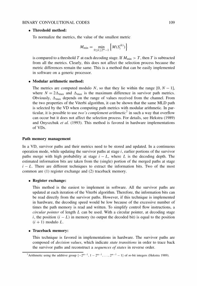
BINARY CONVOLUTIONAL CODES 109
• Threshold method:
To normalize the metrics, the value of the smallest metric
Mmin = min0≤k≤2m−1
{M(S
(k)i )
}
is compared to a threshold T at each decoding stage. If Mmin > T , then T is subtractedfrom all the metrics. Clearly, this does not affect the selection process because themetric differences remain the same. This is a method that can be easily implementedin software on a generic processor.
• Modular arithmetic method:
The metrics are computed modulo N , so that they lie within the range [0, N − 1],where N = 2�max and �max is the maximum difference in survivor path metrics.Obviously, �max depends on the range of values received from the channel. Fromthe two properties of the Viterbi algorithm, it can be shown that the same MLD pathis selected by the VD when computing path metrics with modular arithmetic. In par-ticular, it is possible to use two’s complement arithmetic7 in such a way that overflowcan occur but it does not affect the selection process. For details, see Hekstra (1989)and Onyszchuk et al. (1993). This method is favored in hardware implementationsof VDs.
Path memory management
In a VD, survivor paths and their metrics need to be stored and updated. In a continuousoperation mode, while updating the survivor paths at stage i, earlier portions of the survivorpaths merge with high probability at stage i − L, where L is the decoding depth. Theestimated information bits are taken from the (single) portion of the merged paths at stagei − L. There are different techniques to extract the information bits. Two of the mostcommon are (1) register exchange and (2) traceback memory.
• Register exchange:
This method is the easiest to implement in software. All the survivor paths areupdated at each iteration of the Viterbi algorithm. Therefore, the information bits canbe read directly from the survivor paths. However, if this technique is implementedin hardware, the decoding speed would be low because of the excessive number oftimes the path memory is read and written. To simplify control flow instructions, acircular pointer of length L can be used. With a circular pointer, at decoding stagei, the position (i − L) in memory (to output the decoded bit) is equal to the position(i + 1) modulo L.
• Traceback memory:
This technique is favored in implementations in hardware. The survivor paths arecomposed of decision values, which indicate state transitions in order to trace backthe survivor paths and reconstruct a sequences of states in reverse order.
7Arithmetic using the additive group {−2m−1, 1 − 2m−1, . . . , 2m−1 − 1} of m-bit integers (Hekstra 1989).
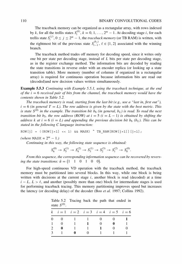
110 BINARY CONVOLUTIONAL CODES
The traceback memory can be organized as a rectangular array, with rows indexedby k, for all the trellis states S
(k)i , k = 0, 1, . . . , 2m − 1. At decoding stage i, for each
trellis state S(j)
i , 0 ≤ j ≤ 2m − 1, the traceback memory (or TB RAM) is written, with
the rightmost bit of the previous state S(bj )
i−1 , � ∈ {1, 2} associated with the winningbranch.
The traceback method trades off memory for decoding speed, since it writes onlyone bit per state per decoding stage, instead of L bits per state per decoding stage,as in the register exchange method. The information bits are decoded by readingthe state transitions in reverse order with an encoder replica (or looking up a statetransition table). More memory (number of columns if organized in a rectangulararray) is required for continuous operation because information bits are read out(decoded)and new decision values written simultaneously.
Example 5.5.3 Continuing with Example 5.5.1, using the traceback technique, at the endof the i = 6 received pair of bits from the channel, the traceback memory would have thecontents shown in Table 5.2.
The traceback memory is read, starting from the last bit (e.g., use a “last in, first out”),i = 6 (in general T = L). The row address is given by the state with the best metric. Thisis state S(0) in the example. The transition bit b6 (in general, bL) is read. To read the nexttransition bit b5, the row address (ROW) at i = 5 (i = L − 1) is obtained by shifting theaddress k at i = 6 (i = L) and appending the previous decision bit b6 (bL). This can bestated in the following C language instruction:
ROW[j] = ((ROW[j+1] << 1) && MASK) ^ TB_RAM[ROW[j+1]][j+1];
(where MASK = 2m − 1.)Continuing in this way, the following state sequence is obtained:
S(0)6 → S
(1)5 → S
(2)4 → S
(1)3 → S
(3)2 → S
(2)1 → S
(0)0 .
From this sequence, the corresponding information sequence can be recovered by revers-ing the state transitions: u = (
1 1 0 1 0 0).
For high-speed continuous VD operation with the traceback method, the tracebackmemory must be partitioned into several blocks. In this way, while one block is beingwritten with decisions at the current stage i, another block is read (decoded) at a timei − L, L > �, and another (possibly more than one) block for intermediate stages is usedfor performing traceback tracing. This memory partitioning improves speed but increasesthe latency (or decoding delay) of the decoder (Boo et al. 1997; Collins 1992).
Table 5.2 Tracing back the path that ended instate S(0).
k i = 1 i = 2 i = 3 i = 4 i = 5 i = 6
0 0 1 1 0 0 11 0 1 1 0 0 12 0 1 1 1 0 03 1 0 0 1 1 1
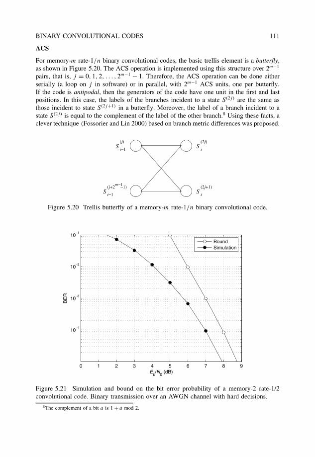
BINARY CONVOLUTIONAL CODES 111
ACS
For memory-m rate-1/n binary convolutional codes, the basic trellis element is a butterfly,as shown in Figure 5.20. The ACS operation is implemented using this structure over 2m−1
pairs, that is, j = 0, 1, 2, . . . , 2m−1 − 1. Therefore, the ACS operation can be done eitherserially (a loop on j in software) or in parallel, with 2m−1 ACS units, one per butterfly.If the code is antipodal, then the generators of the code have one unit in the first and lastpositions. In this case, the labels of the branches incident to a state S(2j) are the same asthose incident to state S(2j+1) in a butterfly. Moreover, the label of a branch incident to astate S(2j) is equal to the complement of the label of the other branch.8 Using these facts, aclever technique (Fossorier and Lin 2000) based on branch metric differences was proposed.
S
S
i−1S(j) (2j)
i
(2j+1)
iS
i−1
(j+2 −1)m−1
Figure 5.20 Trellis butterfly of a memory-m rate-1/n binary convolutional code.
0 1 2 3 4 5 6 7 8 9
10−4
10−3
10−2
10−1
Eb/N
0 (dB)
BE
R
BoundSimulation
Figure 5.21 Simulation and bound on the bit error probability of a memory-2 rate-1/2convolutional code. Binary transmission over an AWGN channel with hard decisions.
8The complement of a bit a is 1 + a mod 2.
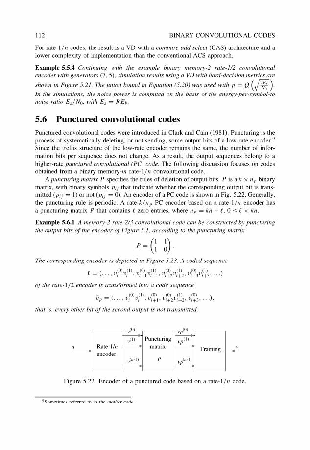
112 BINARY CONVOLUTIONAL CODES
For rate-1/n codes, the result is a VD with a compare-add-select (CAS) architecture and alower complexity of implementation than the conventional ACS approach.
Example 5.5.4 Continuing with the example binary memory-2 rate-1/2 convolutionalencoder with generators (7, 5), simulation results using a VD with hard-decision metrics are
shown in Figure 5.21. The union bound in Equation (5.20) was used with p = Q(√
2Es
N0
).
In the simulations, the noise power is computed on the basis of the energy-per-symbol-tonoise ratio Es/N0, with Es = REb.
5.6 Punctured convolutional codesPunctured convolutional codes were introduced in Clark and Cain (1981). Puncturing is theprocess of systematically deleting, or not sending, some output bits of a low-rate encoder.9
Since the trellis structure of the low-rate encoder remains the same, the number of infor-mation bits per sequence does not change. As a result, the output sequences belong to ahigher-rate punctured convolutional (PC) code. The following discussion focuses on codesobtained from a binary memory-m rate-1/n convolutional code.
A puncturing matrix P specifies the rules of deletion of output bits. P is a k × np binarymatrix, with binary symbols pij that indicate whether the corresponding output bit is trans-mitted (pij = 1) or not (pij = 0). An encoder of a PC code is shown in Fig. 5.22. Generally,the puncturing rule is periodic. A rate-k/np PC encoder based on a rate-1/n encoder hasa puncturing matrix P that contains � zero entries, where np = kn − �, 0 ≤ � < kn.
Example 5.6.1 A memory-2 rate-2/3 convolutional code can be constructed by puncturingthe output bits of the encoder of Figure 5.1, according to the puncturing matrix
P =(
1 11 0
).
The corresponding encoder is depicted in Figure 5.23. A coded sequence
v = (. . . , v(0)i v
(1)i , v
(0)i+1v
(1)i+1, v
(0)i+2v
(1)i+2, v
(0)i+3v
(1)i+3, . . .)
of the rate-1/2 encoder is transformed into a code sequence
vp = (. . . , v(0)i v
(1)i , v
(0)i+1, v
(0)i+2v
(1)i+2, v
(0)i+3, . . .),
that is, every other bit of the second output is not transmitted.
encoderRate-1/n
Puncturingmatrix
P
u
v vp
v
v
vp
vp
(0)
(1)
(n-1)
(0)
(1)
(n-1)
Framing v
Figure 5.22 Encoder of a punctured code based on a rate-1/n code.
9Sometimes referred to as the mother code.
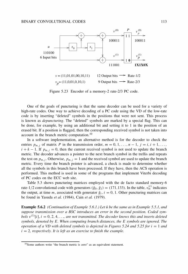
BINARY CONVOLUTIONAL CODES 113
v = (11,0,01,0,10,1)p 9 Output bits Rate-2/3
12 Output bits Rate-1/2v = (11,01,01,00,10,11)
u
110100
100011
111001
1 1
P
100011
1X1X0X1 0
6 Input bits v
v v
v
(0)
(1)
(0)
(1)p
p
s s0 1
Figure 5.23 Encoder of a memory-2 rate-2/3 PC code.
One of the goals of puncturing is that the same decoder can be used for a variety ofhigh-rate codes. One way to achieve decoding of a PC code using the VD of the low-ratecode is by inserting “deleted” symbols in the positions that were not sent. This processis known as depuncturing. The “deleted” symbols are marked by a special flag. This canbe done, for example, by using an additional bit and setting it to 1 in the position of anerased bit. If a position is flagged, then the corresponding received symbol is not taken intoaccount in the branch metric computation.10
In a software implementation, an alternative method is for the decoder to check theentries pm,j of matrix P in the transmission order, m = 0, 1, . . . , n − 1, j = i, i + 1, . . . ,
i + k − 1. If pm,j = 0, then the current received symbol is not used to update the branchmetric. The decoder advances a pointer to the next branch symbol in the trellis and repeatsthe test on pm,j . Otherwise, pm,j = 1 and the received symbol are used to update the branchmetric. Every time the branch pointer is advanced, a check is made to determine whetherall the symbols in this branch have been processed. If they have, then the ACS operation isperformed. This method is used in some of the programs that implement Viterbi decodingof PC codes on the ECC web site.
Table 5.3 shows puncturing matrices employed with the de facto standard memory-6rate-1/2 convolutional code with generators (g0, g1) = (171,133). In the table, v
(i)m indicates
the output, at time m, associated with generator gi , i = 0, 1. Other puncturing matrices canbe found in Yasuda et al. (1984), Cain et al. (1979).
Example 5.6.2 (Continuation of Example 5.6.1.) Let u be the same as in Example 5.5.1, andsuppose transmission over a BSC introduces an error in the second position. Coded sym-bols v(1)[i], i = 0, 2, 4, . . ., are not transmitted. The decoder knows this and inserts deletedsymbols, denoted by E. When computing branch distances, the E symbols are ignored. Theoperation of a VD with deleted symbols is depicted in Figures 5.24 and 5.25 for i = 1 andi = 2, respectively. It is left as an exercise to finish the example.
10Some authors write “the branch metric is zero” as an equivalent statement.
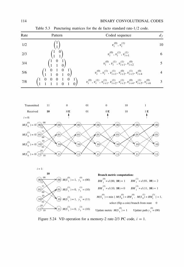
114 BINARY CONVOLUTIONAL CODES
Table 5.3 Puncturing matrices for the de facto standard rate-1/2 code.
Rate Pattern Coded sequence df
1/2
(11
)v
(0)i , v
(1)i 10
2/3
(1 01 1
)v
(0)i , v
(1)i , v
(1)i+1 6
3/4
(1 0 11 1 0
)v
(0)i , v
(1)i , v
(1)i+1, v
(0)i+2 5
5/6
(1 0 1 0 11 1 0 1 0
)v
(0)i , v
(1)i , v
(1)i+1, v
(0)i+2, v
(1)i+3, v
(0)i+4 4
7/8
(1 0 0 0 1 0 11 1 1 1 0 1 0
)v
(0)i , v
(1)i , v
(1)i+1, v
(1)i+2, v
(1)i+3, v
(0)i+4, v
(1)i+5, v
(0)i+6 3
01 10
01 0 10
10
11
00
01
10
11
00
01
10
11
00
01
10
11
00
01
10
11
00
01
10
11
00
01
10
11
00
11
00
10
01
10
00
01
10
11
00
11
11
00
10
01
01
10
00
01
10
11
10
1
(0) (0)
1M(S ) = 1,
1 1
1 1M(S ) = 1,
1 1
(1)M(S ) = 0, y = (10)
(1)
(2) (2)
(3) (3)M(S ) = 0, y = (10)
0
0 E 0 E 1 E
1
y = (00)
y = (11)
00
01
10
11
11
01
Transmitted
Received
i = 1:
Branch metric computation:
1 10(0)
BM = d (00, ) = 11 10
1 10 1 10
(1)
(2) (3)
(0)
1M(S ) = min { M(S ) + BM , M(S ) + BM } = 1,0 0
(0) (1)(0) (3)
1 1
Update metric M(S ) = 1(0)
1 1
(0)
select (flip a coin) branch from state 0
Update path y = (00)
BM = d (01, ) = 2
BM = d (10, ) = 0 BM = d (11, ) = 1
i = 0:
M(S ) = 00
M(S ) = 0
M(S ) = 0
M(S ) = 00
0
0
(0)
(1)
(2)
(3)
Figure 5.24 VD operation for a memory-2 rate-2/3 PC code, i = 1.
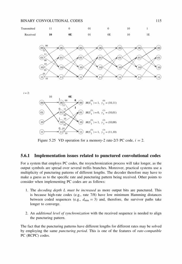
BINARY CONVOLUTIONAL CODES 115
Transmitted
Received 01 10
01 10 1
10
11
00
01
10
11
00
01
10
11
00
01
10
11
00
01
10
11
00
01
10
11
00
11
00
10
01
10
00
01
10
11
00
01
10
11
10i = 2:
00
01
10
11
1
0
1
0
(0) (0)M(S ) = 1,
M(S ) = 1,
(1)M(S ) = 0,
(1)
(2) (2)
(3) (3)
2 2
2 2
2 2
2 2
y = (10,11)
y = (10,01)
y = (10,00)
M(S ) = 1,
0E 0E 1E
0 0
0E
1
0
y = (11,10)
00
01
10
11
11
01
00
01
10
11
00
11
11
00
10
01
01
10
Figure 5.25 VD operation for a memory-2 rate-2/3 PC code, i = 2.
5.6.1 Implementation issues related to punctured convolutional codes
For a system that employs PC codes, the resynchronization process will take longer, as theoutput symbols are spread over several trellis branches. Moreover, practical systems use amultiplicity of puncturing patterns of different lengths. The decoder therefore may have tomake a guess as to the specific rate and puncturing pattern being received. Other points toconsider when implementing PC codes are as follows:
1. The decoding depth L must be increased as more output bits are punctured. Thisis because high-rate codes (e.g., rate 7/8) have low minimum Hamming distancesbetween coded sequences (e.g., dmin = 3) and, therefore, the survivor paths takelonger to converge.
2. An additional level of synchronization with the received sequence is needed to alignthe puncturing pattern.
The fact that the puncturing patterns have different lengths for different rates may be solvedby employing the same puncturing period. This is one of the features of rate-compatiblePC (RCPC) codes.
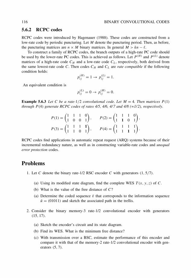
116 BINARY CONVOLUTIONAL CODES
5.6.2 RCPC codes
RCPC codes were introduced by Hagenauer (1988). These codes are constructed from alow-rate code by periodic puncturing. Let M denote the puncturing period. Then, as before,the puncturing matrices are n × M binary matrices. In general M > kn − �.
To construct a family of RCPC codes, the branch outputs of a high-rate PC code shouldbe used by the lower-rate PC codes. This is achieved as follows. Let P (H) and P (L) denotematrices of a high-rate code CH and a low-rate code CL, respectively, both derived fromthe same lowest-rate code C. Then codes CH and CL are rate compatible if the followingcondition holds:
p(H)ij = 1 → p
(L)ij = 1.
An equivalent condition is
p(L)ij = 0 → p
(H)ij = 0.
Example 5.6.3 Let C be a rate-1/2 convolutional code. Let M = 4. Then matrices P (1)
through P (4) generate RCPC codes of rates 4/5, 4/6, 4/ 7 and 4/8 (=1/ 2), respectively.
P (1) =(
1 1 1 01 0 0 1
), P (2) =
(1 1 1 01 1 0 1
),
P (3) =(
1 1 1 11 1 0 1
), P (4) =
(1 1 1 11 1 1 1
).
RCPC codes find applications in automatic repeat request (ARQ) systems because of theirincremental redundancy nature, as well as in constructing variable-rate codes and unequalerror protection codes.
Problems
1. Let C denote the binary rate-1/2 RSC encoder C with generators (1, 5/7).
(a) Using its modified state diagram, find the complete WES T (x, y, z) of C.
(b) What is the value of the free distance of C?
(a) Determine the coded sequence v that corresponds to the information sequenceu = (01011) and sketch the associated path in the trellis.
2. Consider the binary memory-3 rate-1/2 convolutional encoder with generators(15, 17).
(a) Sketch the encoder’s circuit and its state diagram.
(b) Find its WES. What is the minimum free distance?
(c) With transmission over a BSC, estimate the performance of this encoder andcompare it with that of the memory-2 rate-1/2 convolutional encoder with gen-erators (5, 7).
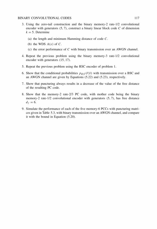
BINARY CONVOLUTIONAL CODES 117
3. Using the zero-tail construction and the binary memory-2 rate-1/2 convolutionalencoder with generators (5, 7), construct a binary linear block code C of dimensionk = 5. Determine
(a) the length and minimum Hamming distance of code C.
(b) the WDS A(x) of C.
(c) the error performance of C with binary transmission over an AWGN channel.
4. Repeat the previous problem using the binary memory-3 rate-1/2 convolutionalencoder with generators (15, 17).
5. Repeat the previous problem using the RSC encoder of problem 1.
6. Show that the conditional probabilities pR|V (r|v) with transmission over a BSC andan AWGN channel are given by Equations (5.22) and (5.23), respectively.
7. Show that puncturing always results in a decrease of the value of the free distanceof the resulting PC code.
8. Show that the memory-2 rate-2/3 PC code, with mother code being the binarymemory-2 rate-1/2 convolutional encoder with generators (5, 7), has free distancedf = 6.
9. Simulate the performance of each of the five memory-6 PCCs with puncturing matri-ces given in Table 5.3, with binary transmission over an AWGN channel, and compareit with the bound in Equation (5.20).
6
Modifying and combining codes
In this chapter, several techniques are presented that allow modification of an existing code,or the combination of several codes, in order to achieve flexibility in the design of errorcorrecting codes (ECC). Many of the best codes known to date have been obtained not frommembers of a known family of codes, but from modifying and combining codes (Brouwerand Verhoeff 1993).
6.1 Modifying codes
In the following, let C denote a linear block (n, k, d) code over GF(q) with generatormatrix G and parity-check matrix H .
6.1.1 Shortening
Shortened cyclic codes were described in Section 3.1.5. Let s be an integer, 0 ≤ s < k.In general, a linear shortened (n − s, k − s, ds) code Cs has distance ds ≥ d. A generatormatrix of Cs can be obtained from the generator matrix G of the original code C as follows.Assume that G is in systematic form, that is,
G = (Ik|P
). (6.1)
Then a (k − s) × (n − s) generator matrix Gs of the shortened code Cs is obtained byremoving s columns of the identity matrix Ik and the s rows that correspond to where theselected columns elements are nonzero. This is best illustrated by an example.
Example 6.1.1 Consider the Hamming (7, 4, 3) code, presented in Example 2.1.1. Thiscode has
G =
1 0 0 0 1 0 10 1 0 0 1 1 10 0 1 0 1 1 00 0 0 1 0 1 1
. (6.2)
The Art of Error Correcting Coding, Second Edition Robert H. Morelos-Zaragoza 2006 John Wiley & Sons, Ltd. ISBN: 0-470-01558-6
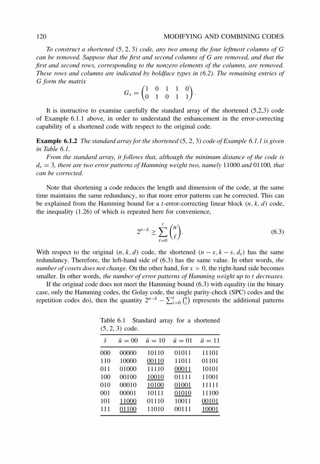
120 MODIFYING AND COMBINING CODES
To construct a shortened (5, 2, 3) code, any two among the four leftmost columns of G
can be removed. Suppose that the first and second columns of G are removed, and that thefirst and second rows, corresponding to the nonzero elements of the columns, are removed.These rows and columns are indicated by boldface types in (6.2). The remaining entries ofG form the matrix
Gs =(
1 0 1 1 00 1 0 1 1
).
It is instructive to examine carefully the standard array of the shortened (5,2,3) codeof Example 6.1.1 above, in order to understand the enhancement in the error-correctingcapability of a shortened code with respect to the original code.
Example 6.1.2 The standard array for the shortened (5, 2, 3) code of Example 6.1.1 is givenin Table 6.1.
From the standard array, it follows that, although the minimum distance of the code isds = 3, there are two error patterns of Hamming weight two, namely 11000 and 01100, thatcan be corrected.
Note that shortening a code reduces the length and dimension of the code, at the sametime maintains the same redundancy, so that more error patterns can be corrected. This canbe explained from the Hamming bound for a t-error-correcting linear block (n, k, d) code,the inequality (1.26) of which is repeated here for convenience,
2n−k ≥t∑
�=0
(n
�
). (6.3)
With respect to the original (n, k, d) code, the shortened (n − s, k − s, ds) has the sameredundancy. Therefore, the left-hand side of (6.3) has the same value. In other words, thenumber of cosets does not change. On the other hand, for s > 0, the right-hand side becomessmaller. In other words, the number of error patterns of Hamming weight up to t decreases.
If the original code does not meet the Hamming bound (6.3) with equality (in the binarycase, only the Hamming codes, the Golay code, the single parity-check (SPC) codes and therepetition codes do), then the quantity 2n−k − ∑t
i=0
(ni
)represents the additional patterns
Table 6.1 Standard array for a shortened(5, 2, 3) code.
s u = 00 u = 10 u = 01 u = 11
000 00000 10110 01011 11101110 10000 00110 11011 01101011 01000 11110 00011 10101100 00100 10010 01111 11001010 00010 10100 01001 11111001 00001 10111 01010 11100101 11000 01110 10011 00101111 01100 11010 00111 10001
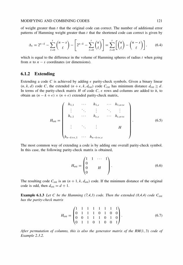
MODIFYING AND COMBINING CODES 121
of weight greater than t that the original code can correct. The number of additional errorpatterns of Hamming weight greater than t that the shortened code can correct is given by
�t = 2n−k −t∑
�=0
(n − s
�
)−
[2n−k −
t∑�=0
(n
�
)]=
t∑�=0
[(n
�
)−
(n − s
�
)], (6.4)
which is equal to the difference in the volume of Hamming spheres of radius t when goingfrom n to n − s coordinates (or dimensions).
6.1.2 Extending
Extending a code C is achieved by adding ε parity-check symbols. Given a binary linear(n, k, d) code C, the extended (n + ε, k, dext) code Cext has minimum distance dext ≥ d .In terms of the parity-check matrix H of code C, ε rows and columns are added to it, toobtain an (n − k + ε) × (n + ε) extended parity-check matrix,
Hext =
h1,1 · · · h1,ε · · · h1,n+ε
.... . .
.... . .
...
hε,1 · · · hε,ε · · · hε,n+ε
.... . .
... H
hn−k+ε,1 · · · hn−k+ε,ε
. (6.5)
The most common way of extending a code is by adding one overall parity-check symbol.In this case, the following parity-check matrix is obtained,
Hext =
1 1 · · · 100 H
0
. (6.6)
The resulting code Cext is an (n + 1, k, dext) code. If the minimum distance of the originalcode is odd, then dext = d + 1.
Example 6.1.3 Let C be the Hamming (7,4,3) code. Then the extended (8,4,4) code Cext
has the parity-check matrix
Hext =
1 1 1 1 1 1 1 10 1 1 1 0 1 0 00 0 1 1 1 0 1 00 1 1 0 1 0 0 1
. (6.7)
After permutation of columns, this is also the generator matrix of the RM(1, 3) code ofExample 2.3.2.
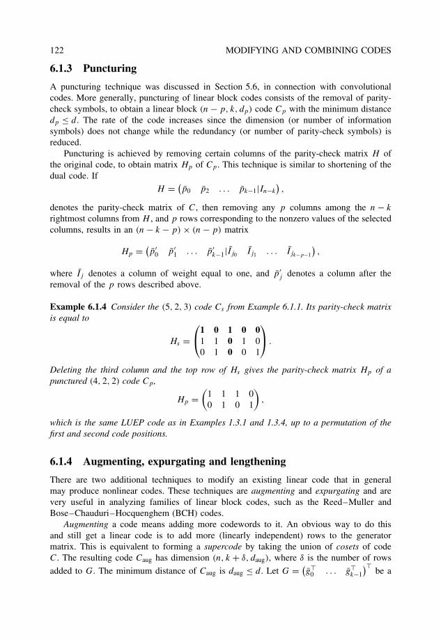
122 MODIFYING AND COMBINING CODES
6.1.3 Puncturing
A puncturing technique was discussed in Section 5.6, in connection with convolutionalcodes. More generally, puncturing of linear block codes consists of the removal of parity-check symbols, to obtain a linear block (n − p, k, dp) code Cp with the minimum distancedp ≤ d . The rate of the code increases since the dimension (or number of informationsymbols) does not change while the redundancy (or number of parity-check symbols) isreduced.
Puncturing is achieved by removing certain columns of the parity-check matrix H ofthe original code, to obtain matrix Hp of Cp. This technique is similar to shortening of thedual code. If
H = (p0 p2 . . . pk−1|In−k
),
denotes the parity-check matrix of C, then removing any p columns among the n − k
rightmost columns from H , and p rows corresponding to the nonzero values of the selectedcolumns, results in an (n − k − p) × (n − p) matrix
Hp = (p′
0 p′1 . . . p′
k−1|Ij0 Ij1 . . . Ijk−p−1
),
where Ij denotes a column of weight equal to one, and p′j denotes a column after the
removal of the p rows described above.
Example 6.1.4 Consider the (5, 2, 3) code Cs from Example 6.1.1. Its parity-check matrixis equal to
Hs =1 0 1 0 0
1 1 0 1 00 1 0 0 1
.
Deleting the third column and the top row of Hs gives the parity-check matrix Hp of apunctured (4, 2, 2) code Cp,
Hp =(
1 1 1 00 1 0 1
),
which is the same LUEP code as in Examples 1.3.1 and 1.3.4, up to a permutation of thefirst and second code positions.
6.1.4 Augmenting, expurgating and lengthening
There are two additional techniques to modify an existing linear code that in generalmay produce nonlinear codes. These techniques are augmenting and expurgating and arevery useful in analyzing families of linear block codes, such as the Reed–Muller andBose–Chauduri–Hocquenghem (BCH) codes.
Augmenting a code means adding more codewords to it. An obvious way to do thisand still get a linear code is to add more (linearly independent) rows to the generatormatrix. This is equivalent to forming a supercode by taking the union of cosets of codeC. The resulting code Caug has dimension (n, k + δ, daug), where δ is the number of rows
added to G. The minimum distance of Caug is daug ≤ d. Let G = (g�
0 . . . g�k−1
)�be a
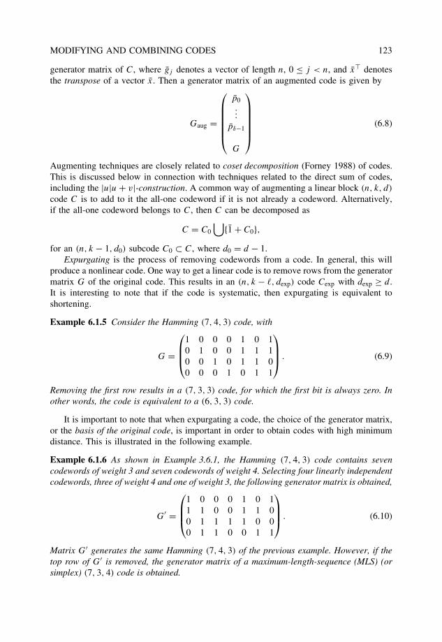
MODIFYING AND COMBINING CODES 123
generator matrix of C, where gj denotes a vector of length n, 0 ≤ j < n, and x� denotesthe transpose of a vector x. Then a generator matrix of an augmented code is given by
Gaug =
p0...
pδ−1
G
(6.8)
Augmenting techniques are closely related to coset decomposition (Forney 1988) of codes.This is discussed below in connection with techniques related to the direct sum of codes,including the |u|u + v|-construction. A common way of augmenting a linear block (n, k, d)
code C is to add to it the all-one codeword if it is not already a codeword. Alternatively,if the all-one codeword belongs to C, then C can be decomposed as
C = C0
⋃{1 + C0},
for an (n, k − 1, d0) subcode C0 ⊂ C, where d0 = d − 1.Expurgating is the process of removing codewords from a code. In general, this will
produce a nonlinear code. One way to get a linear code is to remove rows from the generatormatrix G of the original code. This results in an (n, k − �, dexp) code Cexp with dexp ≥ d .It is interesting to note that if the code is systematic, then expurgating is equivalent toshortening.
Example 6.1.5 Consider the Hamming (7, 4, 3) code, with
G =
1 0 0 0 1 0 10 1 0 0 1 1 10 0 1 0 1 1 00 0 0 1 0 1 1
. (6.9)
Removing the first row results in a (7, 3, 3) code, for which the first bit is always zero. Inother words, the code is equivalent to a (6, 3, 3) code.
It is important to note that when expurgating a code, the choice of the generator matrix,or the basis of the original code, is important in order to obtain codes with high minimumdistance. This is illustrated in the following example.
Example 6.1.6 As shown in Example 3.6.1, the Hamming (7, 4, 3) code contains sevencodewords of weight 3 and seven codewords of weight 4. Selecting four linearly independentcodewords, three of weight 4 and one of weight 3, the following generator matrix is obtained,
G′ =
1 0 0 0 1 0 11 1 0 0 1 1 00 1 1 1 1 0 00 1 1 0 0 1 1
. (6.10)
Matrix G′ generates the same Hamming (7, 4, 3) of the previous example. However, if thetop row of G′ is removed, the generator matrix of a maximum-length-sequence (MLS) (orsimplex) (7, 3, 4) code is obtained.
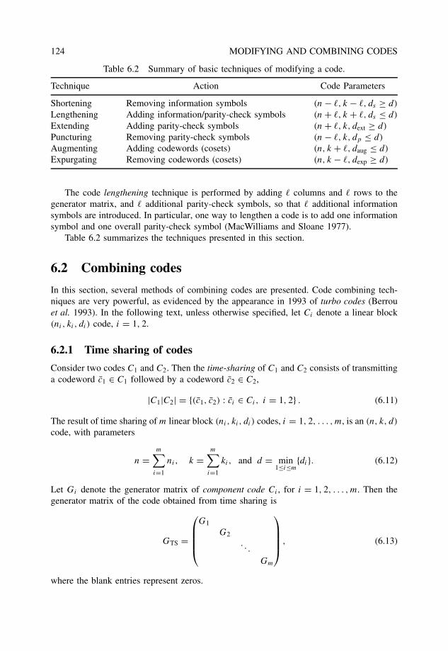
124 MODIFYING AND COMBINING CODES
Table 6.2 Summary of basic techniques of modifying a code.
Technique Action Code Parameters
Shortening Removing information symbols (n − �, k − �, ds ≥ d)
Lengthening Adding information/parity-check symbols (n + �, k + �, ds ≤ d)
Extending Adding parity-check symbols (n + �, k, dext ≥ d)
Puncturing Removing parity-check symbols (n − �, k, dp ≤ d)
Augmenting Adding codewords (cosets) (n, k + �, daug ≤ d)
Expurgating Removing codewords (cosets) (n, k − �, dexp ≥ d)
The code lengthening technique is performed by adding � columns and � rows to thegenerator matrix, and � additional parity-check symbols, so that � additional informationsymbols are introduced. In particular, one way to lengthen a code is to add one informationsymbol and one overall parity-check symbol (MacWilliams and Sloane 1977).
Table 6.2 summarizes the techniques presented in this section.
6.2 Combining codes
In this section, several methods of combining codes are presented. Code combining tech-niques are very powerful, as evidenced by the appearance in 1993 of turbo codes (Berrouet al. 1993). In the following text, unless otherwise specified, let Ci denote a linear block(ni, ki, di) code, i = 1, 2.
6.2.1 Time sharing of codes
Consider two codes C1 and C2. Then the time-sharing of C1 and C2 consists of transmittinga codeword c1 ∈ C1 followed by a codeword c2 ∈ C2,
|C1|C2| = {(c1, c2) : ci ∈ Ci, i = 1, 2} . (6.11)
The result of time sharing of m linear block (ni, ki, di) codes, i = 1, 2, . . . , m, is an (n, k, d)
code, with parameters
n =m∑
i=1
ni, k =m∑
i=1
ki, and d = min1≤i≤m
{di}. (6.12)
Let Gi denote the generator matrix of component code Ci , for i = 1, 2, . . . , m. Then thegenerator matrix of the code obtained from time sharing is
GTS =
G1
G2
. . .
Gm
, (6.13)
where the blank entries represent zeros.
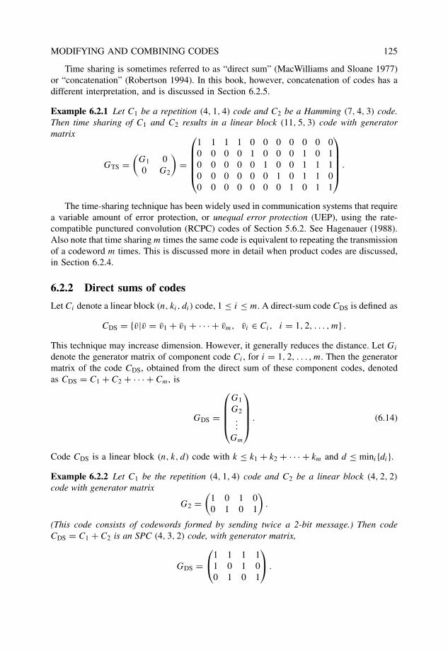
MODIFYING AND COMBINING CODES 125
Time sharing is sometimes referred to as “direct sum” (MacWilliams and Sloane 1977)or “concatenation” (Robertson 1994). In this book, however, concatenation of codes has adifferent interpretation, and is discussed in Section 6.2.5.
Example 6.2.1 Let C1 be a repetition (4, 1, 4) code and C2 be a Hamming (7, 4, 3) code.Then time sharing of C1 and C2 results in a linear block (11, 5, 3) code with generatormatrix
GTS =(
G1 00 G2
)=
1 1 1 1 0 0 0 0 0 0 00 0 0 0 1 0 0 0 1 0 10 0 0 0 0 1 0 0 1 1 10 0 0 0 0 0 1 0 1 1 00 0 0 0 0 0 0 1 0 1 1
.
The time-sharing technique has been widely used in communication systems that requirea variable amount of error protection, or unequal error protection (UEP), using the rate-compatible punctured convolution (RCPC) codes of Section 5.6.2. See Hagenauer (1988).Also note that time sharing m times the same code is equivalent to repeating the transmissionof a codeword m times. This is discussed more in detail when product codes are discussed,in Section 6.2.4.
6.2.2 Direct sums of codes
Let Ci denote a linear block (n, ki, di) code, 1 ≤ i ≤ m. A direct-sum code CDS is defined as
CDS = {v|v = v1 + v1 + · · · + vm, vi ∈ Ci, i = 1, 2, . . . , m} .
This technique may increase dimension. However, it generally reduces the distance. Let Gi
denote the generator matrix of component code Ci , for i = 1, 2, . . . , m. Then the generatormatrix of the code CDS, obtained from the direct sum of these component codes, denotedas CDS = C1 + C2 + · · · + Cm, is
GDS =
G1
G2...
Gm
. (6.14)
Code CDS is a linear block (n, k, d) code with k ≤ k1 + k2 + · · · + km and d ≤ mini{di}.Example 6.2.2 Let C1 be the repetition (4, 1, 4) code and C2 be a linear block (4, 2, 2)
code with generator matrix
G2 =(
1 0 1 00 1 0 1
).
(This code consists of codewords formed by sending twice a 2-bit message.) Then codeCDS = C1 + C2 is an SPC (4, 3, 2) code, with generator matrix,
GDS =1 1 1 1
1 0 1 00 1 0 1
.
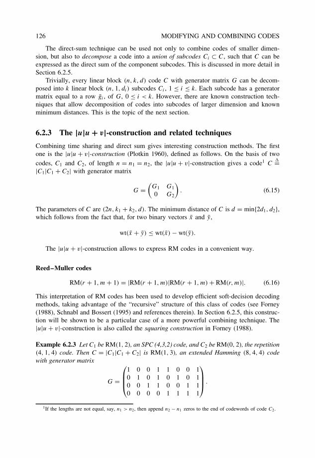
126 MODIFYING AND COMBINING CODES
The direct-sum technique can be used not only to combine codes of smaller dimen-sion, but also to decompose a code into a union of subcodes Ci ⊂ C, such that C can beexpressed as the direct sum of the component subcodes. This is discussed in more detail inSection 6.2.5.
Trivially, every linear block (n, k, d) code C with generator matrix G can be decom-posed into k linear block (n, 1, di) subcodes Ci , 1 ≤ i ≤ k. Each subcode has a generatormatrix equal to a row gi , of G, 0 ≤ i < k. However, there are known construction tech-niques that allow decomposition of codes into subcodes of larger dimension and knownminimum distances. This is the topic of the next section.
6.2.3 The |u|u + v|-construction and related techniques
Combining time sharing and direct sum gives interesting construction methods. The firstone is the |u|u + v|-construction (Plotkin 1960), defined as follows. On the basis of two
codes, C1 and C2, of length n = n1 = n2, the |u|u + v|-construction gives a code1 C�=
|C1|C1 + C2| with generator matrix
G =(
G1 G1
0 G2
). (6.15)
The parameters of C are (2n, k1 + k2, d). The minimum distance of C is d = min{2d1, d2},which follows from the fact that, for two binary vectors x and y,
wt(x + y) ≤ wt(x) − wt(y).
The |u|u + v|-construction allows to express RM codes in a convenient way.
Reed–Muller codes
RM(r + 1, m + 1) = |RM(r + 1, m)|RM(r + 1, m) + RM(r, m)|. (6.16)
This interpretation of RM codes has been used to develop efficient soft-decision decodingmethods, taking advantage of the “recursive” structure of this class of codes (see Forney(1988), Schnabl and Bossert (1995) and references therein). In Section 6.2.5, this construc-tion will be shown to be a particular case of a more powerful combining technique. The|u|u + v|-construction is also called the squaring construction in Forney (1988).
Example 6.2.3 Let C1 be RM(1, 2), an SPC (4,3,2) code, and C2 be RM(0, 2), the repetition(4, 1, 4) code. Then C = |C1|C1 + C2| is RM(1, 3), an extended Hamming (8, 4, 4) codewith generator matrix
G =
1 0 0 1 1 0 0 10 1 0 1 0 1 0 10 0 1 1 0 0 1 10 0 0 0 1 1 1 1
.
1If the lengths are not equal, say, n1 > n2, then append n2 − n1 zeros to the end of codewords of code C2.
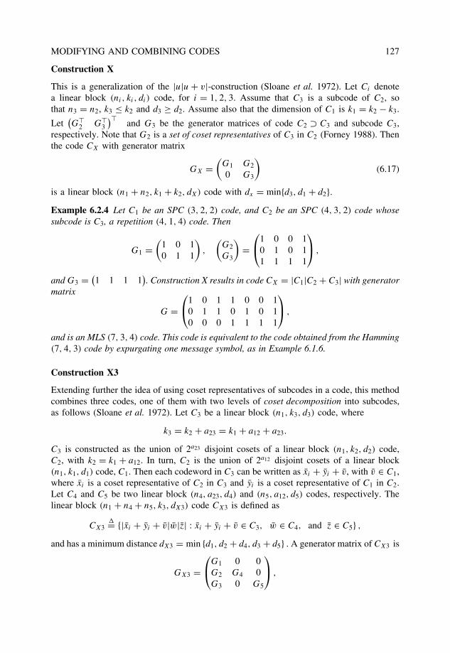
MODIFYING AND COMBINING CODES 127
Construction X
This is a generalization of the |u|u + v|-construction (Sloane et al. 1972). Let Ci denotea linear block (ni, ki, di) code, for i = 1, 2, 3. Assume that C3 is a subcode of C2, sothat n3 = n2, k3 ≤ k2 and d3 ≥ d2. Assume also that the dimension of C1 is k1 = k2 − k3.
Let(G�
2 G�3
)�and G3 be the generator matrices of code C2 ⊃ C3 and subcode C3,
respectively. Note that G2 is a set of coset representatives of C3 in C2 (Forney 1988). Thenthe code CX with generator matrix
GX =(
G1 G2
0 G3
)(6.17)
is a linear block (n1 + n2, k1 + k2, dX) code with dx = min{d3, d1 + d2}.Example 6.2.4 Let C1 be an SPC (3, 2, 2) code, and C2 be an SPC (4, 3, 2) code whosesubcode is C3, a repetition (4, 1, 4) code. Then
G1 =(
1 0 10 1 1
),
(G2
G3
)=
1 0 0 1
0 1 0 11 1 1 1
,
and G3 = (1 1 1 1
). Construction X results in code CX = |C1|C2 + C3| with generator
matrix
G =1 0 1 1 0 0 1
0 1 1 0 1 0 10 0 0 1 1 1 1
,
and is an MLS (7, 3, 4) code. This code is equivalent to the code obtained from the Hamming(7, 4, 3) code by expurgating one message symbol, as in Example 6.1.6.
Construction X3
Extending further the idea of using coset representatives of subcodes in a code, this methodcombines three codes, one of them with two levels of coset decomposition into subcodes,as follows (Sloane et al. 1972). Let C3 be a linear block (n1, k3, d3) code, where
k3 = k2 + a23 = k1 + a12 + a23.
C3 is constructed as the union of 2a23 disjoint cosets of a linear block (n1, k2, d2) code,C2, with k2 = k1 + a12. In turn, C2 is the union of 2a12 disjoint cosets of a linear block(n1, k1, d1) code, C1. Then each codeword in C3 can be written as xi + yi + v, with v ∈ C1,where xi is a coset representative of C2 in C3 and yi is a coset representative of C1 in C2.Let C4 and C5 be two linear block (n4, a23, d4) and (n5, a12, d5) codes, respectively. Thelinear block (n1 + n4 + n5, k3, dX3) code CX3 is defined as
CX3�= {|xi + yi + v|w|z| : xi + yi + v ∈ C3, w ∈ C4, and z ∈ C5} ,
and has a minimum distance dX3 = min {d1, d2 + d4, d3 + d5} . A generator matrix of CX3 is
GX3 =G1 0 0
G2 G4 0G3 0 G5
,
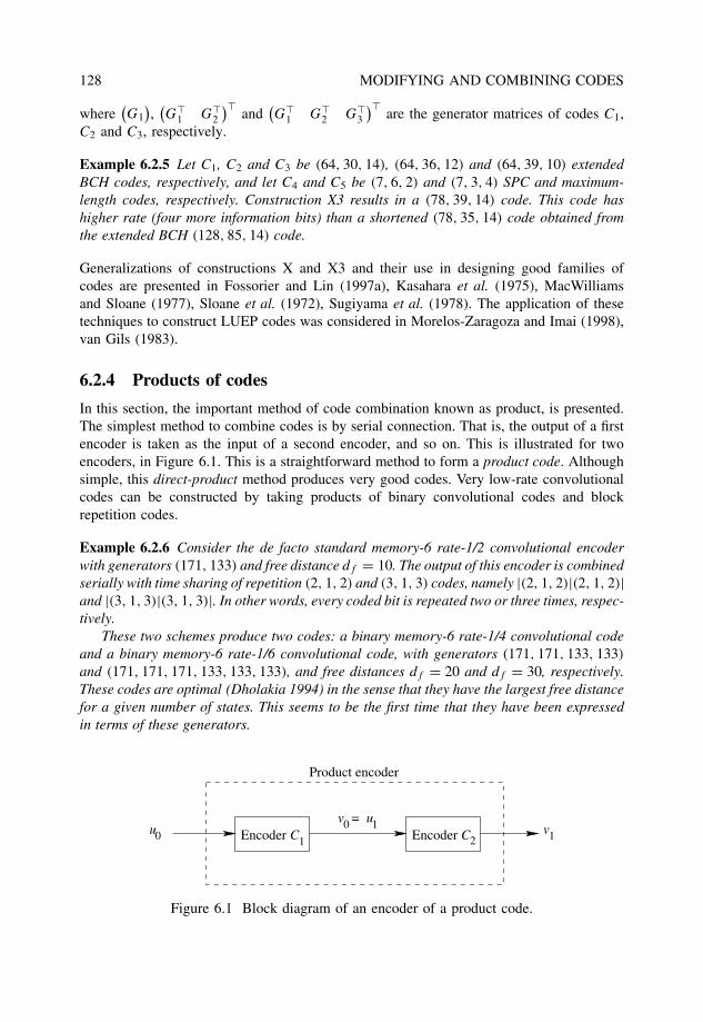
128 MODIFYING AND COMBINING CODES
where(G1
),(G�
1 G�2
)�and
(G�
1 G�2 G�
3
)�are the generator matrices of codes C1,
C2 and C3, respectively.
Example 6.2.5 Let C1, C2 and C3 be (64, 30, 14), (64, 36, 12) and (64, 39, 10) extendedBCH codes, respectively, and let C4 and C5 be (7, 6, 2) and (7, 3, 4) SPC and maximum-length codes, respectively. Construction X3 results in a (78, 39, 14) code. This code hashigher rate (four more information bits) than a shortened (78, 35, 14) code obtained fromthe extended BCH (128, 85, 14) code.
Generalizations of constructions X and X3 and their use in designing good families ofcodes are presented in Fossorier and Lin (1997a), Kasahara et al. (1975), MacWilliamsand Sloane (1977), Sloane et al. (1972), Sugiyama et al. (1978). The application of thesetechniques to construct LUEP codes was considered in Morelos-Zaragoza and Imai (1998),van Gils (1983).
6.2.4 Products of codes
In this section, the important method of code combination known as product, is presented.The simplest method to combine codes is by serial connection. That is, the output of a firstencoder is taken as the input of a second encoder, and so on. This is illustrated for twoencoders, in Figure 6.1. This is a straightforward method to form a product code. Althoughsimple, this direct-product method produces very good codes. Very low-rate convolutionalcodes can be constructed by taking products of binary convolutional codes and blockrepetition codes.
Example 6.2.6 Consider the de facto standard memory-6 rate-1/2 convolutional encoderwith generators (171, 133) and free distance df = 10. The output of this encoder is combinedserially with time sharing of repetition (2, 1, 2) and (3, 1, 3) codes, namely |(2, 1, 2)|(2, 1, 2)|and |(3, 1, 3)|(3, 1, 3)|. In other words, every coded bit is repeated two or three times, respec-tively.
These two schemes produce two codes: a binary memory-6 rate-1/4 convolutional codeand a binary memory-6 rate-1/6 convolutional code, with generators (171, 171, 133, 133)
and (171, 171, 171, 133, 133, 133), and free distances df = 20 and df = 30, respectively.These codes are optimal (Dholakia 1994) in the sense that they have the largest free distancefor a given number of states. This seems to be the first time that they have been expressedin terms of these generators.
u0
uv =0 1 v1
Product encoder
Encoder C Encoder C1 2
Figure 6.1 Block diagram of an encoder of a product code.
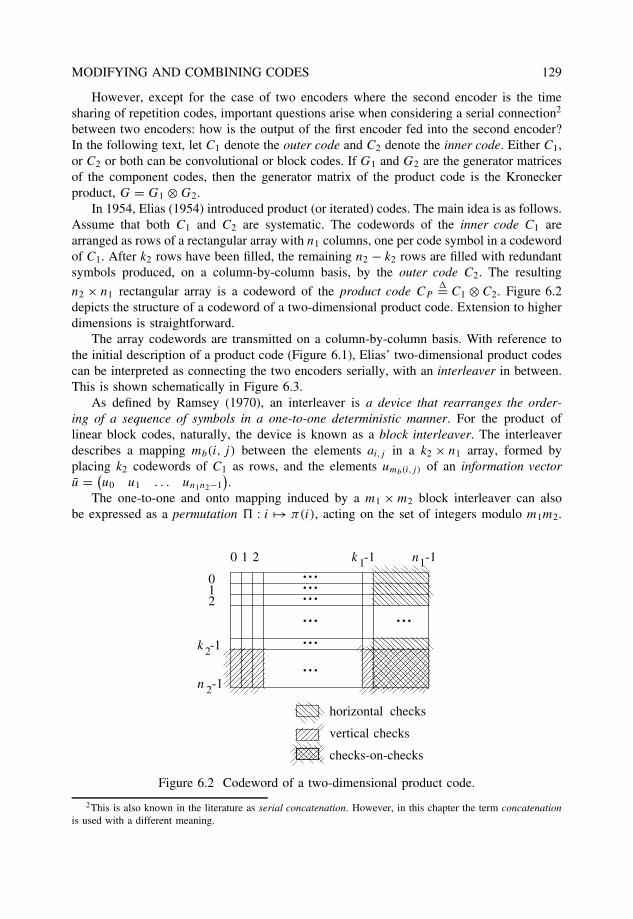
MODIFYING AND COMBINING CODES 129
However, except for the case of two encoders where the second encoder is the timesharing of repetition codes, important questions arise when considering a serial connection2
between two encoders: how is the output of the first encoder fed into the second encoder?In the following text, let C1 denote the outer code and C2 denote the inner code. Either C1,or C2 or both can be convolutional or block codes. If G1 and G2 are the generator matricesof the component codes, then the generator matrix of the product code is the Kroneckerproduct, G = G1 ⊗ G2.
In 1954, Elias (1954) introduced product (or iterated) codes. The main idea is as follows.Assume that both C1 and C2 are systematic. The codewords of the inner code C1 arearranged as rows of a rectangular array with n1 columns, one per code symbol in a codewordof C1. After k2 rows have been filled, the remaining n2 − k2 rows are filled with redundantsymbols produced, on a column-by-column basis, by the outer code C2. The resulting
n2 × n1 rectangular array is a codeword of the product code CP�= C1 ⊗ C2. Figure 6.2
depicts the structure of a codeword of a two-dimensional product code. Extension to higherdimensions is straightforward.
The array codewords are transmitted on a column-by-column basis. With reference tothe initial description of a product code (Figure 6.1), Elias’ two-dimensional product codescan be interpreted as connecting the two encoders serially, with an interleaver in between.This is shown schematically in Figure 6.3.
As defined by Ramsey (1970), an interleaver is a device that rearranges the order-ing of a sequence of symbols in a one-to-one deterministic manner. For the product oflinear block codes, naturally, the device is known as a block interleaver. The interleaverdescribes a mapping mb(i, j) between the elements ai,j in a k2 × n1 array, formed byplacing k2 codewords of C1 as rows, and the elements umb(i,j) of an information vectoru = (
u0 u1 . . . un1n2−1).
The one-to-one and onto mapping induced by a m1 × m2 block interleaver can alsobe expressed as a permutation � : i → π(i), acting on the set of integers modulo m1m2.
k -10 1 2
0 12
k -1
n -1
n -1
11
2
2
checks-on-checks
vertical checks
horizontal checks
...
...
...
.........
...
Figure 6.2 Codeword of a two-dimensional product code.
2This is also known in the literature as serial concatenation. However, in this chapter the term concatenationis used with a different meaning.
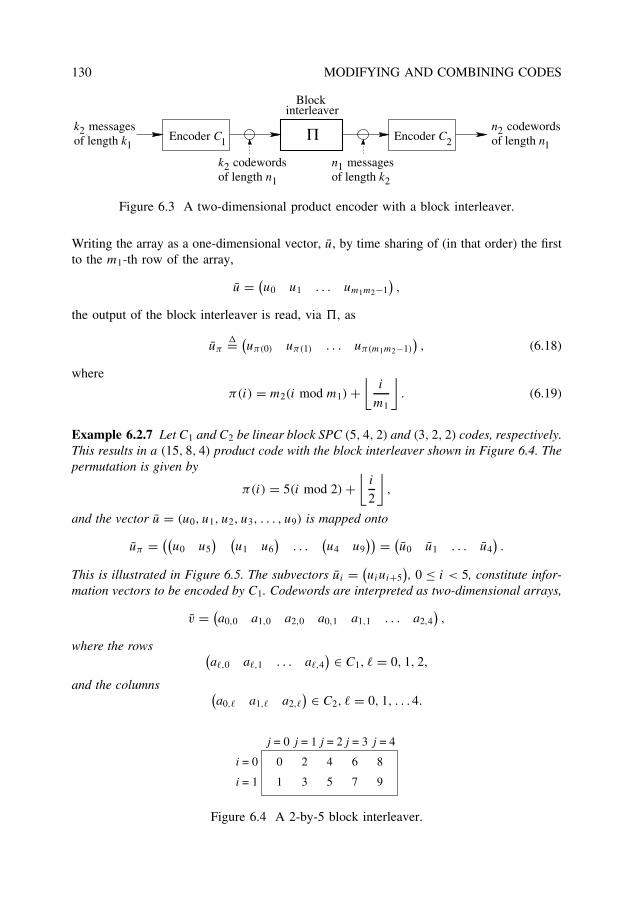
130 MODIFYING AND COMBINING CODES
Encoder C1 Πinterleaver
Block
Encoder C2
n codewordsof length n1
2
n messagesof length k2
1k codewordsof length n1
2
k messagesof length k1
2
Figure 6.3 A two-dimensional product encoder with a block interleaver.
Writing the array as a one-dimensional vector, u, by time sharing of (in that order) the firstto the m1-th row of the array,
u = (u0 u1 . . . um1m2−1
),
the output of the block interleaver is read, via �, as
uπ�= (
uπ(0) uπ(1) . . . uπ(m1m2−1)
), (6.18)
where
π(i) = m2(i mod m1) +⌊
i
m1
⌋. (6.19)
Example 6.2.7 Let C1 and C2 be linear block SPC (5, 4, 2) and (3, 2, 2) codes, respectively.This results in a (15, 8, 4) product code with the block interleaver shown in Figure 6.4. Thepermutation is given by
π(i) = 5(i mod 2) +⌊
i
2
⌋,
and the vector u = (u0, u1, u2, u3, . . . , u9) is mapped onto
uπ = ((u0 u5
) (u1 u6
). . .
(u4 u9
)) = (u0 u1 . . . u4
).
This is illustrated in Figure 6.5. The subvectors ui = (uiui+5
), 0 ≤ i < 5, constitute infor-
mation vectors to be encoded by C1. Codewords are interpreted as two-dimensional arrays,
v = (a0,0 a1,0 a2,0 a0,1 a1,1 . . . a2,4
),
where the rows (a�,0 a�,1 . . . a�,4
) ∈ C1, � = 0, 1, 2,
and the columns (a0,� a1,� a2,�
) ∈ C2, � = 0, 1, . . . 4.
0 i = 0
i = 1
j = 0 j = 1 j = 2 j = 3 j = 4
1
2
3
4
5
6
7
8
9
Figure 6.4 A 2-by-5 block interleaver.
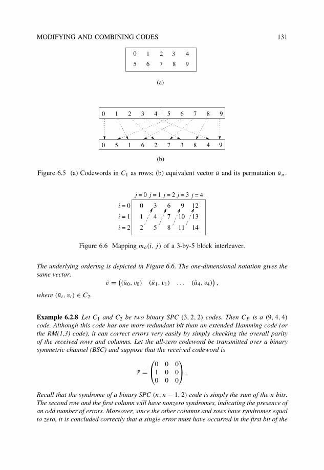
MODIFYING AND COMBINING CODES 131
0 1 2 3 4
95 6 7 8
0 1 2 3 4 95 6 7 8
0 5 1 6 2 7 3 4 98
(b)
(a)
Figure 6.5 (a) Codewords in C1 as rows; (b) equivalent vector u and its permutation uπ .
0
2
4
3
8
7
i = 0
i = 1
i = 2
9
10
j = 0 j = 1 j = 2 j = 3 j = 4
1
5
6
11 14
13
12
Figure 6.6 Mapping mb(i, j) of a 3-by-5 block interleaver.
The underlying ordering is depicted in Figure 6.6. The one-dimensional notation gives thesame vector,
v = ((u0, v0) (u1, v1) . . . (u4, v4)
),
where (ui, vi) ∈ C2.
Example 6.2.8 Let C1 and C2 be two binary SPC (3, 2, 2) codes. Then CP is a (9, 4, 4)
code. Although this code has one more redundant bit than an extended Hamming code (orthe RM(1,3) code), it can correct errors very easily by simply checking the overall parityof the received rows and columns. Let the all-zero codeword be transmitted over a binarysymmetric channel (BSC) and suppose that the received codeword is
r =0 0 0
1 0 00 0 0
.
Recall that the syndrome of a binary SPC (n, n − 1, 2) code is simply the sum of the n bits.The second row and the first column will have nonzero syndromes, indicating the presence ofan odd number of errors. Moreover, since the other columns and rows have syndromes equalto zero, it is concluded correctly that a single error must have occurred in the first bit of the
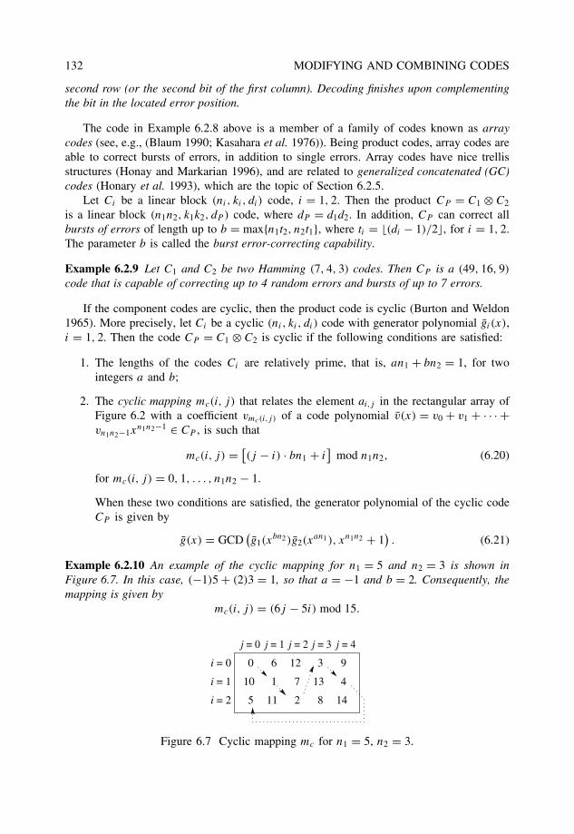
132 MODIFYING AND COMBINING CODES
second row (or the second bit of the first column). Decoding finishes upon complementingthe bit in the located error position.
The code in Example 6.2.8 above is a member of a family of codes known as arraycodes (see, e.g., (Blaum 1990; Kasahara et al. 1976)). Being product codes, array codes areable to correct bursts of errors, in addition to single errors. Array codes have nice trellisstructures (Honay and Markarian 1996), and are related to generalized concatenated (GC)codes (Honary et al. 1993), which are the topic of Section 6.2.5.
Let Ci be a linear block (ni, ki, di) code, i = 1, 2. Then the product CP = C1 ⊗ C2
is a linear block (n1n2, k1k2, dP ) code, where dP = d1d2. In addition, CP can correct allbursts of errors of length up to b = max{n1t2, n2t1}, where ti = �(di − 1)/2�, for i = 1, 2.The parameter b is called the burst error-correcting capability.
Example 6.2.9 Let C1 and C2 be two Hamming (7, 4, 3) codes. Then CP is a (49, 16, 9)
code that is capable of correcting up to 4 random errors and bursts of up to 7 errors.
If the component codes are cyclic, then the product code is cyclic (Burton and Weldon1965). More precisely, let Ci be a cyclic (ni, ki, di) code with generator polynomial gi (x),i = 1, 2. Then the code CP = C1 ⊗ C2 is cyclic if the following conditions are satisfied:
1. The lengths of the codes Ci are relatively prime, that is, an1 + bn2 = 1, for twointegers a and b;
2. The cyclic mapping mc(i, j) that relates the element ai,j in the rectangular array ofFigure 6.2 with a coefficient vmc(i,j) of a code polynomial v(x) = v0 + v1 + · · · +vn1n2−1x
n1n2−1 ∈ CP , is such that
mc(i, j) = [(j − i) · bn1 + i
]mod n1n2, (6.20)
for mc(i, j) = 0, 1, . . . , n1n2 − 1.
When these two conditions are satisfied, the generator polynomial of the cyclic codeCP is given by
g(x) = GCD(g1(x
bn2)g2(xan1), xn1n2 + 1
). (6.21)
Example 6.2.10 An example of the cyclic mapping for n1 = 5 and n2 = 3 is shown inFigure 6.7. In this case, (−1)5 + (2)3 = 1, so that a = −1 and b = 2. Consequently, themapping is given by
mc(i, j) = (6j − 5i) mod 15.
0
5
10 1
6
11 2
7
12i = 0
i = 1
i = 2
3
8
13 4
9
14
j = 0 j = 1 j = 2 j = 3 j = 4
Figure 6.7 Cyclic mapping mc for n1 = 5, n2 = 3.
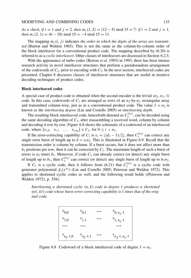
MODIFYING AND COMBINING CODES 133
As a check, if i = 1 and j = 2, then mc(1, 2) = (12 − 5) mod 15 = 7; if i = 2 and j = 1,then mc(2, 1) = (6 − 10) mod 15 = −4 mod 15 = 11.
The mapping mc(i, j) indicates the order in which the digits of the array are transmit-ted (Burton and Weldon 1965). This is not the same as the column-by-column order ofthe block interleaver for a conventional product code. The mapping described by (6.20) isreferred to as a cyclic interleaver. Other classes of interleavers are discussed in Section 6.2.5.
With the appearance of turbo codes (Berrou et al. 1993) in 1993, there has been intenseresearch activity in novel interleaver structures that perform a pseudorandom arrangementof the codewords of C1, prior to encoding with C2. In the next section, interleaved codes arepresented. Chapter 8 discusses classes of interleaver structures that are useful in iterativedecoding techniques of product codes.
Block interleaved codes
A special case of product code is obtained when the second encoder is the trivial (n2, n2, 1)
code. In this case, codewords of C1 are arranged as rows of an n2-by-n1 rectangular arrayand transmitted column-wise, just as in a conventional product code. The value I = n2 isknown as the interleaving degree (Lin and Costello 2005) or interleaving depth.
The resulting block interleaved code, henceforth denoted as C(n2)
1 , can be decoded usingthe same decoding algorithm of C1, after reassembling a received word, column by columnand decoding it row by row. Figure 6.8 shows the schematic of a codeword of an interleavedcode, where
(vi,0 vi,1 . . . vi,n0
) ∈ C1, for 0 ≤ i < n2.
If the error-correcting capability of C1 is t1 = �(d1 − 1)/2�, then C(n2)
1 can correct anysingle error burst of length up to b = t1n2. This is illustrated in Figure 6.9. Recall that thetransmission order is column by column. If a burst occurs, but it does not affect more thanb1 positions per row, then it can be corrected by C1. The maximum length of such a burst oferrors is n2 times b1. Moreover, if code C1 can already correct (or detect) any single burstof length up to b1, then C
(n2)
1 can correct (or detect) any single burst of length up to b1n2.If C1 is a cyclic code, then it follows from (6.21) that C
(n2)
1 is a cyclic code withgenerator polynomial g1(x
n2) (Lin and Costello 2005; Peterson and Weldon 1972). Thisapplies to shortened cyclic codes as well, and the following result holds ((Peterson andWeldon 1972), p. 358):
Interleaving a shortened cyclic (n, k) code to degree � produces a shortened(n�, k�) code whose burst error-correcting capability is � times that of the orig-inal code.
vn -1,0
v1,0
v0,0
vn -1,1 vn -1, n -1
v1,1 v1, n -11
v0,1 v0, n -11
1222
...
...
...... ... ...
Figure 6.8 Codeword of a block interleaved code of degree I = n2.
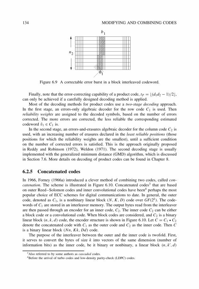
134 MODIFYING AND COMBINING CODES
b
b1
1
2n
Figure 6.9 A correctable error burst in a block interleaved codeword.
Finally, note that the error-correcting capability of a product code, tP = �(d1d2 − 1)/2�,can only be achieved if a carefully designed decoding method is applied.
Most of the decoding methods for product codes use a two-stage decoding approach.In the first stage, an errors-only algebraic decoder for the row code C1 is used. Thenreliability weights are assigned to the decoded symbols, based on the number of errorscorrected. The more errors are corrected, the less reliable the corresponding estimatedcodeword v1 ∈ C1 is.
In the second stage, an errors-and-erasures algebraic decoder for the column code C2 isused, with an increasing number of erasures declared in the least reliable positions (thosepositions for which the reliability weights are the smallest), until a sufficient conditionon the number of corrected errors is satisfied. This is the approach originally proposedin Reddy and Robinson (1972), Weldon (1971). The second decoding stage is usuallyimplemented with the generalized minimum distance (GMD) algorithm, which is discussedin Section 7.6. More details on decoding of product codes can be found in Chapter 8.
6.2.5 Concatenated codes
In 1966, Forney (1966a) introduced a clever method of combining two codes, called con-catenation. The scheme is illustrated in Figure 6.10. Concatenated codes3 that are basedon outer Reed–Solomon codes and inner convolutional codes have been4 perhaps the mostpopular choice of ECC schemes for digital communications to date. In general, the outercode, denoted as C1, is a nonbinary linear block (N, K, D) code over GF(2k). The code-words of C1 are stored in an interleaver memory. The output bytes read from the interleaverare then passed through an encoder for an inner code, C2. The inner code C2 can be eithera block code or a convolutional code. When block codes are considered, and C2 is a binarylinear block (n, k, d) code, the encoder structure is shown in Figure 6.10. Let C = C1 � C2
denote the concatenated code with C1 as the outer code and C2 as the inner code. Then C
is a binary linear block (Nn, Kk, Dd) code.The purpose of the interleaver between the outer and the inner code is twofold. First,
it serves to convert the bytes of size k into vectors of the same dimension (number ofinformation bits) as the inner code, be it binary or nonbinary, a linear block (n, k′, d)
3Also referred to by some authors as cascaded codes.4Before the arrival of turbo codes and low-density parity-check (LDPC) codes.
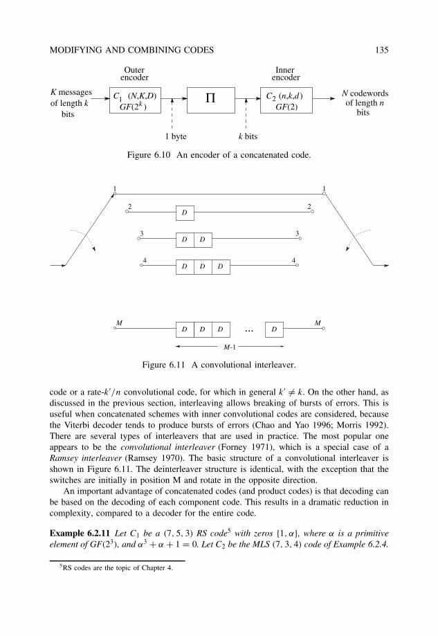
MODIFYING AND COMBINING CODES 135
Outer
kC1 (N,K,D)
GF(2 )Π
Inner
C2
encoder
GF(2)(n,k,d )
encoder
k bits1 byte
N codewordsK messagesof length k
bitsof length n
bits
Figure 6.10 An encoder of a concatenated code.
...
2
3
1
D
D
D
D D
D
D
D
D D
1
2
3
4 4
M M
M-1
Figure 6.11 A convolutional interleaver.
code or a rate-k′/n convolutional code, for which in general k′ = k. On the other hand, asdiscussed in the previous section, interleaving allows breaking of bursts of errors. This isuseful when concatenated schemes with inner convolutional codes are considered, becausethe Viterbi decoder tends to produce bursts of errors (Chao and Yao 1996; Morris 1992).There are several types of interleavers that are used in practice. The most popular oneappears to be the convolutional interleaver (Forney 1971), which is a special case of aRamsey interleaver (Ramsey 1970). The basic structure of a convolutional interleaver isshown in Figure 6.11. The deinterleaver structure is identical, with the exception that theswitches are initially in position M and rotate in the opposite direction.
An important advantage of concatenated codes (and product codes) is that decoding canbe based on the decoding of each component code. This results in a dramatic reduction incomplexity, compared to a decoder for the entire code.
Example 6.2.11 Let C1 be a (7, 5, 3) RS code5 with zeros {1, α}, where α is a primitiveelement of GF(23), and α3 + α + 1 = 0. Let C2 be the MLS (7, 3, 4) code of Example 6.2.4.
5RS codes are the topic of Chapter 4.
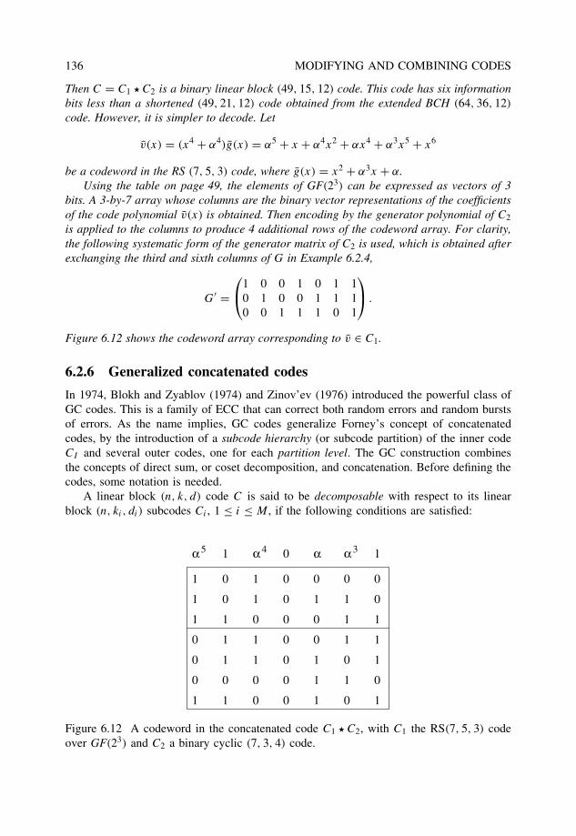
136 MODIFYING AND COMBINING CODES
Then C = C1 � C2 is a binary linear block (49, 15, 12) code. This code has six informationbits less than a shortened (49, 21, 12) code obtained from the extended BCH (64, 36, 12)
code. However, it is simpler to decode. Let
v(x) = (x4 + α4)g(x) = α5 + x + α4x2 + αx4 + α3x5 + x6
be a codeword in the RS (7, 5, 3) code, where g(x) = x2 + α3x + α.Using the table on page 49, the elements of GF(23) can be expressed as vectors of 3
bits. A 3-by-7 array whose columns are the binary vector representations of the coefficientsof the code polynomial v(x) is obtained. Then encoding by the generator polynomial of C2
is applied to the columns to produce 4 additional rows of the codeword array. For clarity,the following systematic form of the generator matrix of C2 is used, which is obtained afterexchanging the third and sixth columns of G in Example 6.2.4,
G′ =1 0 0 1 0 1 1
0 1 0 0 1 1 10 0 1 1 1 0 1
.
Figure 6.12 shows the codeword array corresponding to v ∈ C1.
6.2.6 Generalized concatenated codes
In 1974, Blokh and Zyablov (1974) and Zinov’ev (1976) introduced the powerful class ofGC codes. This is a family of ECC that can correct both random errors and random burstsof errors. As the name implies, GC codes generalize Forney’s concept of concatenatedcodes, by the introduction of a subcode hierarchy (or subcode partition) of the inner codeCI and several outer codes, one for each partition level. The GC construction combinesthe concepts of direct sum, or coset decomposition, and concatenation. Before defining thecodes, some notation is needed.
A linear block (n, k, d) code C is said to be decomposable with respect to its linearblock (n, ki, di) subcodes Ci , 1 ≤ i ≤ M , if the following conditions are satisfied:
1
1
1
0
0
0
1
α5
0
0
1
1
1
0
1
1 0
0
0
0
0
0
0
0
α
0
1
0
1
3α
1
1
0
1
0
1
0
0
1
1
1
4α
1
0
1
1
0
0
0
1
0
1
1
1
0
1
Figure 6.12 A codeword in the concatenated code C1 � C2, with C1 the RS(7, 5, 3) codeover GF(23) and C2 a binary cyclic (7, 3, 4) code.
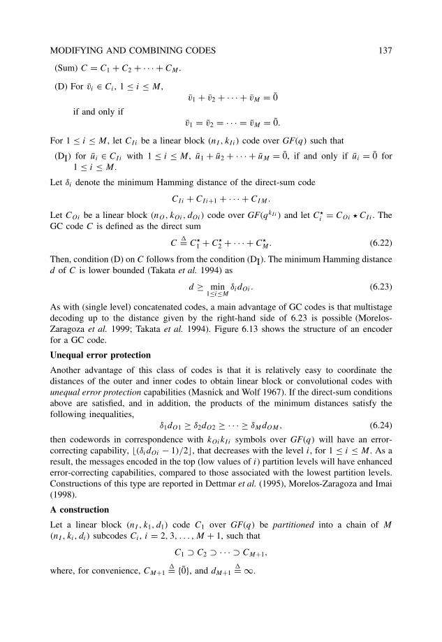
MODIFYING AND COMBINING CODES 137
(Sum) C = C1 + C2 + · · · + CM .
(D) For vi ∈ Ci , 1 ≤ i ≤ M ,v1 + v2 + · · · + vM = 0
if and only ifv1 = v2 = · · · = vM = 0.
For 1 ≤ i ≤ M , let CIi be a linear block (nI , kIi) code over GF(q) such that
(DI) for ui ∈ CIi with 1 ≤ i ≤ M , u1 + u2 + · · · + uM = 0, if and only if ui = 0 for1 ≤ i ≤ M .
Let δi denote the minimum Hamming distance of the direct-sum code
CIi + CIi+1 + · · · + CIM.
Let COi be a linear block (nO, kOi, dOi) code over GF(qkIi ) and let C�i = COi � CIi . The
GC code C is defined as the direct sum
C�= C�
1 + C�2 + · · · + C�
M. (6.22)
Then, condition (D) on C follows from the condition (DI). The minimum Hamming distanced of C is lower bounded (Takata et al. 1994) as
d ≥ min1≤i≤M
δidOi. (6.23)
As with (single level) concatenated codes, a main advantage of GC codes is that multistagedecoding up to the distance given by the right-hand side of 6.23 is possible (Morelos-Zaragoza et al. 1999; Takata et al. 1994). Figure 6.13 shows the structure of an encoderfor a GC code.
Unequal error protection
Another advantage of this class of codes is that it is relatively easy to coordinate thedistances of the outer and inner codes to obtain linear block or convolutional codes withunequal error protection capabilities (Masnick and Wolf 1967). If the direct-sum conditionsabove are satisfied, and in addition, the products of the minimum distances satisfy thefollowing inequalities,
δ1dO1 ≥ δ2dO2 ≥ · · · ≥ δMdOM, (6.24)
then codewords in correspondence with kOikIi symbols over GF(q) will have an error-correcting capability, �(δidOi − 1)/2�, that decreases with the level i, for 1 ≤ i ≤ M . As aresult, the messages encoded in the top (low values of i) partition levels will have enhancederror-correcting capabilities, compared to those associated with the lowest partition levels.Constructions of this type are reported in Dettmar et al. (1995), Morelos-Zaragoza and Imai(1998).
A construction
Let a linear block (nI , k1, d1) code C1 over GF(q) be partitioned into a chain of M
(nI , ki, di) subcodes Ci , i = 2, 3, . . . , M + 1, such that
C1 ⊃ C2 ⊃ · · · ⊃ CM+1,
where, for convenience, CM+1�= {0}, and dM+1
�= ∞.
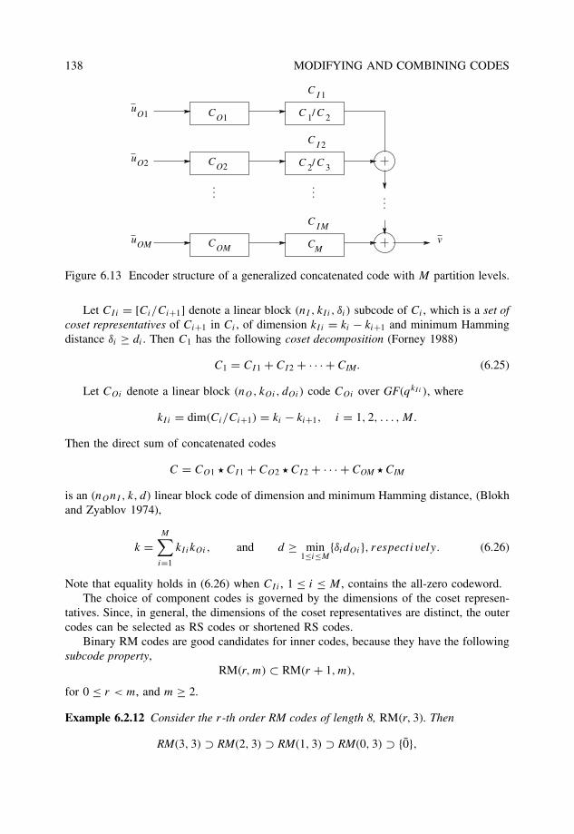
138 MODIFYING AND COMBINING CODES
O1
2O
OMO
O
O
M
2
1
v
...... ...
C 1/ C 2
C I 1
C I 2
C 2/ C 3
C I
MC
M
C
C
Cu
u
u
Figure 6.13 Encoder structure of a generalized concatenated code with M partition levels.
Let CIi = [Ci/Ci+1] denote a linear block (nI , kIi, δi) subcode of Ci , which is a set ofcoset representatives of Ci+1 in Ci , of dimension kIi = ki − ki+1 and minimum Hammingdistance δi ≥ di . Then C1 has the following coset decomposition (Forney 1988)
C1 = CI1 + CI2 + · · · + CIM. (6.25)
Let COi denote a linear block (nO, kOi, dOi) code COi over GF(qkIi ), where
kIi = dim(Ci/Ci+1) = ki − ki+1, i = 1, 2, . . . , M.
Then the direct sum of concatenated codes
C = CO1 � CI1 + CO2 � CI2 + · · · + COM � CIM
is an (nOnI , k, d) linear block code of dimension and minimum Hamming distance, (Blokhand Zyablov 1974),
k =M∑i=1
kIikOi, and d ≥ min1≤i≤M
{δidOi}, respectively. (6.26)
Note that equality holds in (6.26) when CIi , 1 ≤ i ≤ M , contains the all-zero codeword.The choice of component codes is governed by the dimensions of the coset represen-
tatives. Since, in general, the dimensions of the coset representatives are distinct, the outercodes can be selected as RS codes or shortened RS codes.
Binary RM codes are good candidates for inner codes, because they have the followingsubcode property,
RM(r, m) ⊂ RM(r + 1, m),
for 0 ≤ r < m, and m ≥ 2.
Example 6.2.12 Consider the r-th order RM codes of length 8, RM(r, 3). Then
RM(3, 3) ⊃ RM(2, 3) ⊃ RM(1, 3) ⊃ RM(0, 3) ⊃ {0},
MODIFYING AND COMBINING CODES 139
and it follows from (6.25) that
RM(3, 3) = [RM(3, 3)/RM(2, 3)] + [RM(2, 3)/RM(1, 3)]+ [RM(1, 3)/RM(0, 3)] + RM(0, 3).
This decomposition can also be appreciated from the generator matrix of RM(3, 3),expressed as
G =
G1
G2
G3
G4
=
0 0 0 0 0 0 0 1
0 0 0 0 0 0 1 10 0 0 0 0 1 0 10 0 0 1 0 0 0 1
0 0 0 0 1 1 1 10 0 1 1 0 0 1 10 1 0 1 0 1 0 1
1 1 1 1 1 1 1 1
,
where Gi has been defined as the generator matrix of the set of coset representatives ofRM(3 − i, 3) in RM(3 − i + 1, 3), or [RM(3 − i + 1, m)/RM(3 − i, m)], for i = 1, 2, 3, andwhere G4 is the generator matrix of RM(0, 3).
According to this partition of RM(3, 3), a GC code can be designed with up to four levels.Note that the outer codes should be over GF(2), for the first and fourth partition levels, andover GF(23) for the second and third partition levels.
Also, some of the subcodes of RM(3, 3) themselves can be used as inner codes to obtaina GC code with a reduced number of levels. If RM(2, 3) is used as the inner code of a GCcode, then the number of partition levels is three, as the generator matrix of RM(2, 3) isobtained from that of RM(3, 3) by removing G1 (the top row).
Let RM(2, 3) be selected as the inner code, and an RS (8, 1, 8) code CO1 over GF(23),an RS (8, 5, 4) code CO2 over GF(23), and a binary linear SPC (8, 7, 2) code CO3 as theouter code. This gives a binary linear GC (64, 25, 16) code which has one more informationbit than the binary extended BCH (64, 24, 16) code.
It is now shown how Reed–Muller codes can be expressed as GC codes. Recall fromSection 6.2.2, Equation (6.16), that the (r + 1)-th order RM code of length 2m+1 can beexpressed as
RM(r + 1, m + 1) = |RM(r + 1, m)|RM(r + 1, m) + RM(r, m)|.Let G(r, m) denote the generator matrix of RM(r, m). Then
G(r + 1, m + 1) =(
G(r + 1, m) G(r + 1, m)
0 G(r, m)
)
= G(r + 1, m)
(1 10 0
)+ G(r, m)
(0 00 1
). (6.27)
This expression holds for each r-th order RM code, with r ≥ 1 and m > 1, so thata recursion is obtained. From (6.27) it follows that RM(r + 1, m + 1) is a GC code
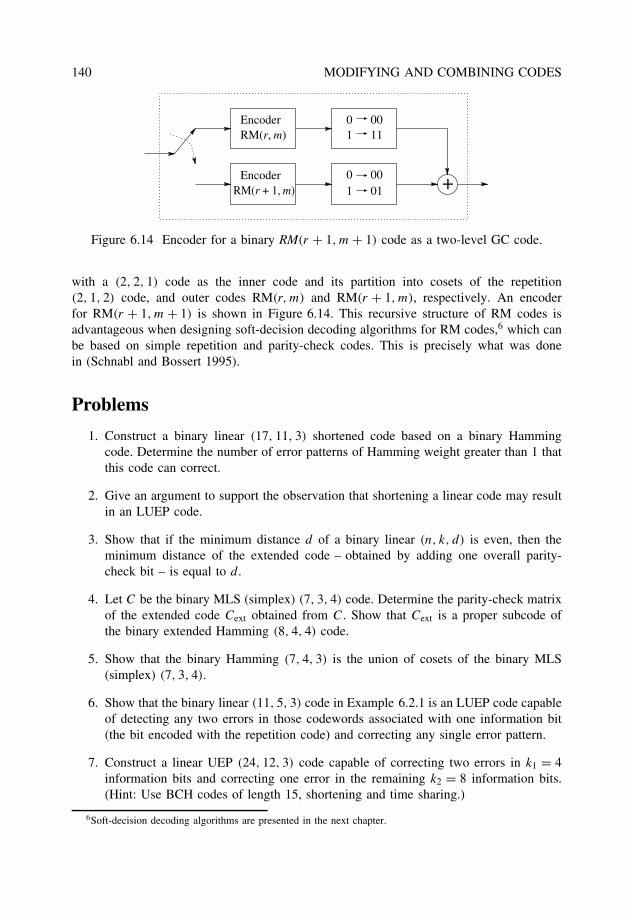
140 MODIFYING AND COMBINING CODES
0 001 11
0 00
1 01
RM(r, m)Encoder
EncoderRM(r + 1, m) +
Figure 6.14 Encoder for a binary RM(r + 1, m + 1) code as a two-level GC code.
with a (2, 2, 1) code as the inner code and its partition into cosets of the repetition(2, 1, 2) code, and outer codes RM(r, m) and RM(r + 1, m), respectively. An encoderfor RM(r + 1, m + 1) is shown in Figure 6.14. This recursive structure of RM codes isadvantageous when designing soft-decision decoding algorithms for RM codes,6 which canbe based on simple repetition and parity-check codes. This is precisely what was donein (Schnabl and Bossert 1995).
Problems
1. Construct a binary linear (17, 11, 3) shortened code based on a binary Hammingcode. Determine the number of error patterns of Hamming weight greater than 1 thatthis code can correct.
2. Give an argument to support the observation that shortening a linear code may resultin an LUEP code.
3. Show that if the minimum distance d of a binary linear (n, k, d) is even, then theminimum distance of the extended code – obtained by adding one overall parity-check bit – is equal to d.
4. Let C be the binary MLS (simplex) (7, 3, 4) code. Determine the parity-check matrixof the extended code Cext obtained from C. Show that Cext is a proper subcode ofthe binary extended Hamming (8, 4, 4) code.
5. Show that the binary Hamming (7, 4, 3) is the union of cosets of the binary MLS(simplex) (7, 3, 4).
6. Show that the binary linear (11, 5, 3) code in Example 6.2.1 is an LUEP code capableof detecting any two errors in those codewords associated with one information bit(the bit encoded with the repetition code) and correcting any single error pattern.
7. Construct a linear UEP (24, 12, 3) code capable of correcting two errors in k1 = 4information bits and correcting one error in the remaining k2 = 8 information bits.(Hint: Use BCH codes of length 15, shortening and time sharing.)
6Soft-decision decoding algorithms are presented in the next chapter.
MODIFYING AND COMBINING CODES 141
8. Show that the direct sum C = C1 ⊕ C2, using a repetition (2m, 1, 2m) code C1 andan extended simplex (2m, m, 2m−1) code C2, is the first-order RM code of length 2m.
9. Find the generator matrix of the code obtained from construction X with C1 as anSPC (4, 3, 2) code and C2 as an SPC (8, 7, 2) code that contains as a proper subcodean extended Hamming (8, 4, 4) code C3.
10. Show that the generator matrix G of the direct product of two linear codes of generatormatrices G1 and G2 is equal to the Kronecker product G = G1 ⊗ G2.
11. Show that the direct-product code CP = C1 ⊗ C2 can correct all bursts of errors oflength up to b = max{n1t2, n2t1}, where ti = �(di − 1)/2�, for i = 1, 2.
12. Design the decoder of an interleaved cyclic code CI with generator polynomialg(xI ) that uses the decoder of the original cyclic code C with generator polynomialg(x). Apply this result to an interleaved cyclic (21, 12, 3) code based on a cyclicHamming (7, 4, 3) code interleaved to degree I = 3. Give a block diagram of thedecoder.
13. Show that the minimum distance of a concatenated code with an outer (N, K, D)
code and an inner (n, k, d) is equal to Dd.
14. Let C = C1 � C2, where C1 is an RS (7, 5, 3) code over GF(23) and C2 is a binarySPC (4, 3, 2) code. Then C is a binary (28, 15, 6) code. This code has 2 bits less thana shortened (28, 17, 6) code that is obtained from an extended BCH (32, 21, 6) code.Devise a decoding algorithm for this code based on a two-stage approach, where thepositions in the RS code where the overall parity-check bit fails are erased. Use anerrors-and-erasures decoding algorithm for the RS code.
7
Soft-decision decoding
In this chapter, decoding with soft information from the channel is considered. For simplicityof exposition, binary transmission over an additive white Gaussian noise (AWGN) channelis assumed. In Chapter 9, the general case of multilevel transmission is discussed. Toprovide a motivation for the use of soft-decision decoding, it can be argued that the noiseenvironment in data retrieval or signal reception is continuous in nature, not discrete. Thismeans that the received symbols are (quantized) real numbers (voltages, currents, etc.), andnot binary or GF(2m) symbols.
When making hard decisions on the received symbols, on a symbol-by-symbol basis,errors may be introduced. This is illustrated in Figure 7.1.
Basically, there are two methods of decoding an error correcting code, based on areceived real-valued sequence.
1. Hard-decision decoding (HDD):
When hard decisions are made on the channel values, errors are introduced. The goalof HDD is to correct binary errors induced in the hard-decision process. The firstpart of the book was devoted to different techniques of HDD for linear block codes,cyclic codes, and convolutional codes.
2. Soft-decision decoding (SDD):
In this case, received values from the channel are directly processed by the decoderin order to estimate a code sequence. A special case of SDD is maximum-likelihooddecoding (MLD), in which the most likely code sequence is output by the decoder.An important point to keep in mind here is that SDD needs to know the statistics ofthe channel noise.
In general, SDD is computationally more intensive than HDD. There are two main reasonsfor this. One is that SDD needs to operate on real numbers. In a practical application, thesenumbers will be quantized to a finite number of bits. In some binary transmission systemsover an AWGN channel, it is known that eight quantization levels, or three bits, are adequateto achieve practically the same performance as with unquantized channel values (Massey1974; Onyszchuk et al. 1993).
The Art of Error Correcting Coding, Second Edition Robert H. Morelos-Zaragoza 2006 John Wiley & Sons, Ltd. ISBN: 0-470-01558-6
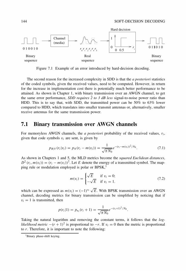
144 SOFT-DECISION DECODING
0 1 0 0 1 0
(media)Channel
r5
r4
r3
r2
r1
r0
Hard decision
ri0 0.5
0
1
0 1 0 1 01
Binary Realsequence sequence
Binarysequence
Figure 7.1 Example of an error introduced by hard-decision decoding.
The second reason for the increased complexity in SDD is that the a posteriori statisticsof the coded symbols, given the received values, need to be computed. However, in returnfor the increase in implementation cost there is potentially much better performance to beattained. As shown in Chapter 1, with binary transmission over an AWGN channel, to getthe same error performance, SDD requires 2 to 3 dB less signal-to-noise power ratio thanHDD. This is to say that, with SDD, the transmitted power can be 50% to 63% lowercompared to HDD, which translates into smaller transmit antennas or, alternatively, smallerreceive antennas for the same transmission power.
7.1 Binary transmission over AWGN channels
For memoryless AWGN channels, the a posteriori probability of the received values, ri ,given that code symbols vi are sent, is given by
pR|V (ri |vi) = pN(ri − m(vi)) = 1√πN0
e−(ri−m(vi ))2/N0 . (7.1)
As shown in Chapters 1 and 5, the MLD metrics become the squared Euclidean distances,D2 (ri, m(vi)) = (ri − m(vi))
2. Let E denote the energy of a transmitted symbol. The map-ping rule or modulation employed is polar or BPSK,1
m(vi) ={√
E if vi = 0;−√
E if vi = 1.(7.2)
which can be expressed as m(vi) = (−1)vi√
E. With BPSK transmission over an AWGNchannel, decoding metrics for binary transmission can be simplified by noticing that ifvi = 1 is transmitted, then
p(ri |1) = pni(ri + 1) = 1√
πN0e−(ri+1)2/N0 .
Taking the natural logarithm and removing the constant terms, it follows that the log-likelihood metric −(r + 1)2 is proportional to −r . If vi = 0 then the metric is proportionalto r . Therefore, it is important to note the following:
1Binary phase-shift keying.
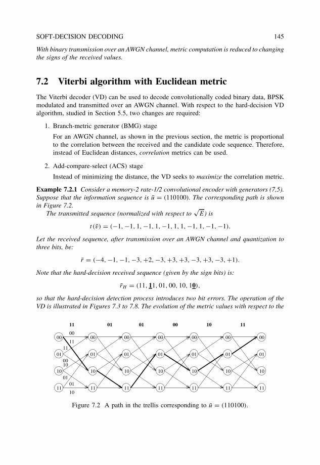
SOFT-DECISION DECODING 145
With binary transmission over an AWGN channel, metric computation is reduced to changingthe signs of the received values.
7.2 Viterbi algorithm with Euclidean metric
The Viterbi decoder (VD) can be used to decode convolutionally coded binary data, BPSKmodulated and transmitted over an AWGN channel. With respect to the hard-decision VDalgorithm, studied in Section 5.5, two changes are required:
1. Branch-metric generator (BMG) stage
For an AWGN channel, as shown in the previous section, the metric is proportionalto the correlation between the received and the candidate code sequence. Therefore,instead of Euclidean distances, correlation metrics can be used.
2. Add-compare-select (ACS) stage
Instead of minimizing the distance, the VD seeks to maximize the correlation metric.
Example 7.2.1 Consider a memory-2 rate-1/2 convolutional encoder with generators (7,5).Suppose that the information sequence is u = (110100). The corresponding path is shownin Figure 7.2.
The transmitted sequence (normalized with respect to√
E) is
t (v) = (−1, −1, 1, −1, 1, −1, 1, 1, −1, 1, −1, −1).
Let the received sequence, after transmission over an AWGN channel and quantization tothree bits, be:
r = (−4, −1, −1, −3, +2, −3, +3, +3, −3, +3, −3, +1).
Note that the hard-decision received sequence (given by the sign bits) is:
rH = (11, 11, 01, 00, 10, 10),
so that the hard-decision detection process introduces two bit errors. The operation of theVD is illustrated in Figures 7.3 to 7.8. The evolution of the metric values with respect to the
00
01
10
11
11
00
10
01
00
11
10
01
00
01
10
11
00
01
10
11
00
01
10
11
00
01
10
11
00
01
10
11
00
01
10
11
11 01 00 10 1101
Figure 7.2 A path in the trellis corresponding to u = (110100).
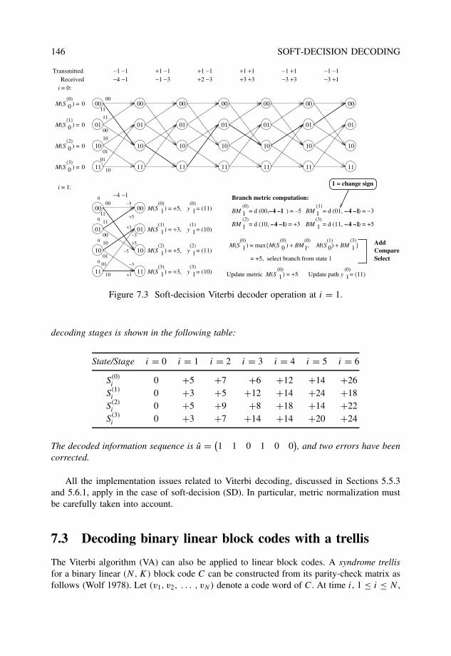
146 SOFT-DECISION DECODING
00
01
10
11
11
01
AddCompareSelect
TransmittedReceived
i = 0:
00
01
10
11
00
01
10
11
00
01
10
11
00
01
10
11
00
01
10
11
M(S ) = 00
M(S ) = 0
M(S ) = 0
00
01
10
11
00
11
00
10
01
10
M(S ) = 00
0
0
00
01
10
11
00
11
11
00
10
01
10
00
01
10
11
−4 −1
(0)
(1)
(2)
(3)
i = 1:
Branch metric computation:
(0)
1 M(S ) + BM }0(1) (3)
1
1 1(0)
1(0)
M(S ) = +5,
1
1
1
(1)
(2)
(3)
−1 −1 +1 −1 +1 −1 +1 +1 −1 +1 −1 −1−4 −1 −1 −3 +2 −3 +3 +3 −3 +3 −3 +1
–4 –1
–4 –1 –4 –1
–4 –1
= +5, select branch from state 1
Update metric M(S ) = +5 Update path y = (11)
(0)
1
1
1
1
y = (10)(1)
(2)
(3)y = (10)
y = (11)
y = (11)
M(S ) = +3,
M(S ) = +5,
M(S ) = +3,
0 1M(S ) = max{M(S ) + BM ,(0) (0)
(0)
1 = change sign
−5
+5
+3
−3
+5
−5
+3
−3
0
0
0
0 01
BM = d (00, ) = –5
BM = d (10, ) = +3
BM = d (01, ) = −3
BM = d (11, ) = +5
1(0)
(2)
1
(1)
1
1(3)
Figure 7.3 Soft-decision Viterbi decoder operation at i = 1.
decoding stages is shown in the following table:
State/Stage i = 0 i = 1 i = 2 i = 3 i = 4 i = 5 i = 6
S(0)i 0 +5 +7 +6 +12 +14 +26
S(1)i 0 +3 +5 +12 +14 +24 +18
S(2)i 0 +5 +9 +8 +18 +14 +22
S(3)i 0 +3 +7 +14 +14 +20 +24
The decoded information sequence is u = (1 1 0 1 0 0
), and two errors have been
corrected.
All the implementation issues related to Viterbi decoding, discussed in Sections 5.5.3and 5.6.1, apply in the case of soft-decision (SD). In particular, metric normalization mustbe carefully taken into account.
7.3 Decoding binary linear block codes with a trellis
The Viterbi algorithm (VA) can also be applied to linear block codes. A syndrome trellisfor a binary linear (N, K) block code C can be constructed from its parity-check matrix asfollows (Wolf 1978). Let (v1, v2, . . . , vN) denote a code word of C. At time i, 1 ≤ i ≤ N ,
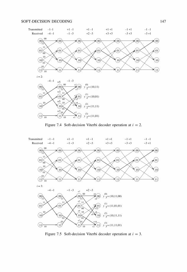
SOFT-DECISION DECODING 147
00
01
10
11
11
01
(0)
(1)
(2)
(3)
y = (10,11)
y = (11,11)
y = (11,01)
2
2
2
2
y = (10,01)
00
01
10
11
00
01
10
11
00
01
10
11
00
01
10
11
00
01
10
11
00
01
10
11
00
11
00
10
01
10
00
01
10
11
–1–1 +1 –1 +1 –1 +1 +1 –1 +1 –1 –1
–4 –1 –1 –3 +2 –3 +3 +3 –3 +3 –3 +1
00
01
10
11
00
11
00
10
01
10
00
01
10
11
–4 –1 –1 –3
+7
+1
+3
01
+5
+3
+5
+3
11
+9–1
+7
+1
11
11
10
10
+5
Transmitted
Received
i = 2:
Figure 7.4 Soft-decision Viterbi decoder operation at i = 2.
00
01
10
11
11
01
(0)
(1)
(2)
(3)
y = (10,11,00)
y = (11,01,01)
y = (10,11,11)
y = (11,11,01)
3
3
3
3
00
01
10
11
00
01
10
11
00
01
10
11
00
01
10
11
00
01
10
11
00
01
10
11
00
11
00
10
01
10
00
01
10
11
−1 −1 +1 −1 +1 −1 +1 +1 −1 +1 −1 −1
−4 −1 −1 −3 +2 −3 +3 +3 −3 +3 −3 +1
00
01
10
11
−4 −1
11
11
10
00
01
10
11
11
01
−1 −3
1100
01
10
11
00
11
00
10
01
10
01
11
+7
+9
+7
+2 −3+6
+4
+12
+8
+14
+2
01
10
+5+6
+4
Transmitted
Received
i = 3:
Figure 7.5 Soft-decision Viterbi decoder operation at i = 3.
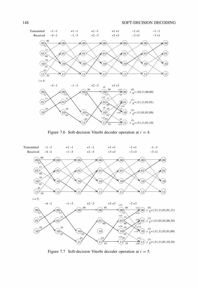
148 SOFT-DECISION DECODING
00
01
10
11
11
01
(0)
(1)
(2)
(3)
y = (10,11,00,00)
y = (11,11,01,01)
y = (11,01,01,00)
y = (11,11,01,10)
4
4
4
4
00
01
10
11
00
01
10
11
00
01
10
11
00
01
10
11
00
01
10
11
00
01
10
11
00
11
00
10
01
10
00
01
10
−1 −1 +1 −1 +1 −1 +1 +1 −1 +1 −1 −1
−4 −1 −1 −3 +2 −3 +3 +3 −3 +3 −3 +1
00
01
10
−4 −1
11
11
10
00
10
11
11
10
01
−1 −3
1100
01
10
11
00
01
01
11
+2 −3
00
01
10
11
00
11
00
10
01
10
01
11
+6
+12
+8
+14
+3 +3+12
+6
+8
+140
+18
+8
+14
Transmitted
Received
i = 4:
Figure 7.6 Soft-decision Viterbi decoder operation at i = 4.
00
01
10
11
11
01
(0)
(1)
(2)
(3)
5
5
5
5
y = (11,01,01,00,10)
y = (11,11,01,01,00)
y = (11,11,01,10,10)
y = (11,11,01,01,11)
00
01
10
11
00
01
10
11
00
01
10
11
00
01
10
11
00
01
10
11
00
01
10
11
00
11
00
10
01
10
00
01
10
−1 −1 +1 −1 +1 −1 +1 +1 −1 +1 −1 −1
−4 −1 −1 −3 +2 −3 +3 +3 −3 +1
00
01
10
−4 −1
11
11
10
00
10
11
11
10
01
−1 −3
1100
01
10
11
00
01
01
+2 −3
00
01
10
11
00
00
10
01
+3 +3
00
01
10
11
00
11
00
10
01
10
01
11
+12
−3 +3
−3 +3+12
+14
+18
+14
+14
+14
+24
+12
+20
+8+12
Transmitted
Received
i = 5:
Figure 7.7 Soft-decision Viterbi decoder operation at i = 5.
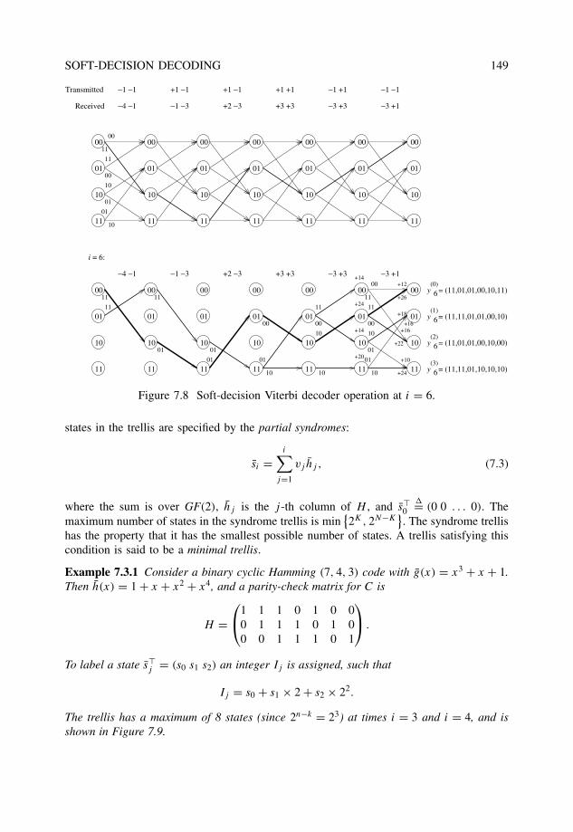
SOFT-DECISION DECODING 149
00
01
10
11
11
01
(0)
(1)
(2)
(3)
6
6
6
6
y = (11,01,01,00,10,11)
y = (11,11,01,01,00,10)
y = (11,01,01,00,10,00)
y = (11,11,01,10,10,10)
00
01
10
11
00
01
10
11
00
01
10
11
00
01
10
11
00
01
10
11
00
01
10
11
00
11
00
10
01
10
00
01
10
11
−1 −1 +1 −1 +1 −1 +1 +1 −1 +1 −1 −1
−4 −1 −1 −3 +2 −3 +3 +3 −3 +1
00
01
10
11
−4 −1
11
11
00
01
10
11
01
−1 −3
1100
01
10
11
01
01
+2 −3
00
01
10
11
00
10
01
+3 +3
−3 +3
00
01
10
11
11
00
10
10
−3 +3
00
01
10
11
00
11
00
10
01
10
01
+12+14
+24
+14
+20
11
−3 +1
+26
+18
+16+16
+22
+10
+24
Transmitted
Received
i = 6:
Figure 7.8 Soft-decision Viterbi decoder operation at i = 6.
states in the trellis are specified by the partial syndromes:
si =i∑
j=1
vj hj , (7.3)
where the sum is over GF(2), hj is the j -th column of H , and s�0
�= (0 0 . . . 0). Themaximum number of states in the syndrome trellis is min
{2K, 2N−K
}. The syndrome trellis
has the property that it has the smallest possible number of states. A trellis satisfying thiscondition is said to be a minimal trellis.
Example 7.3.1 Consider a binary cyclic Hamming (7, 4, 3) code with g(x) = x3 + x + 1.Then h(x) = 1 + x + x2 + x4, and a parity-check matrix for C is
H =1 1 1 0 1 0 0
0 1 1 1 0 1 00 0 1 1 1 0 1
.
To label a state s�j = (s0 s1 s2) an integer Ij is assigned, such that
Ij = s0 + s1 × 2 + s2 × 22.
The trellis has a maximum of 8 states (since 2n−k = 23) at times i = 3 and i = 4, and isshown in Figure 7.9.
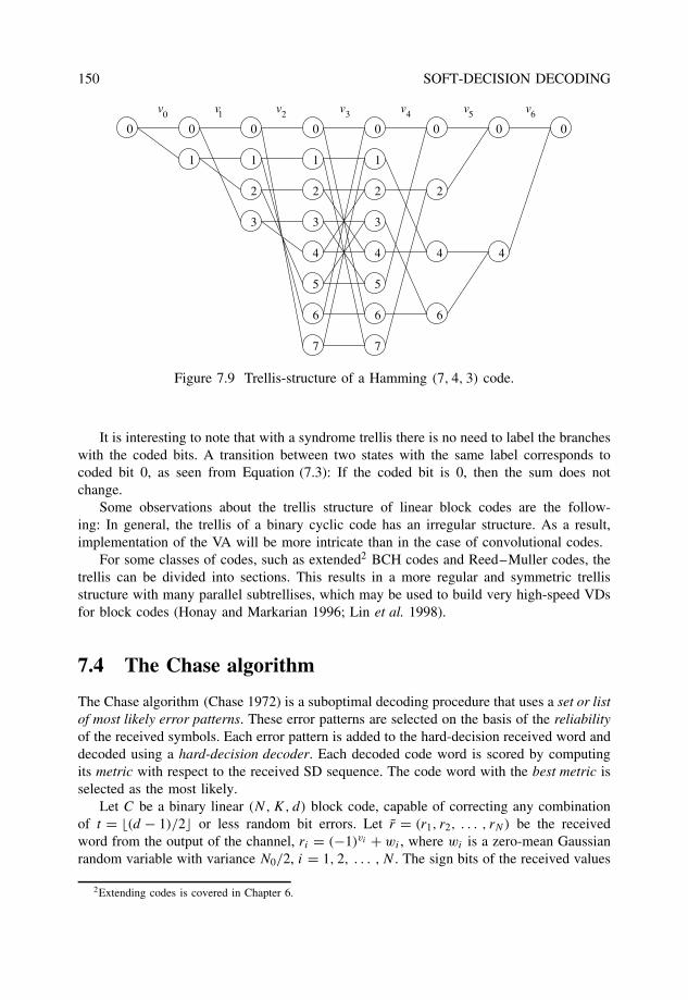
150 SOFT-DECISION DECODING
3
2
3
2
4
5
6
7
3
2
4
5
6
7
0
1
0
1
0
1
0
1
0 0 0 0
2
4
6
4
v0 1 2 3 4 5 6v v v v v v
Figure 7.9 Trellis-structure of a Hamming (7, 4, 3) code.
It is interesting to note that with a syndrome trellis there is no need to label the brancheswith the coded bits. A transition between two states with the same label corresponds tocoded bit 0, as seen from Equation (7.3): If the coded bit is 0, then the sum does notchange.
Some observations about the trellis structure of linear block codes are the follow-ing: In general, the trellis of a binary cyclic code has an irregular structure. As a result,implementation of the VA will be more intricate than in the case of convolutional codes.
For some classes of codes, such as extended2 BCH codes and Reed–Muller codes, thetrellis can be divided into sections. This results in a more regular and symmetric trellisstructure with many parallel subtrellises, which may be used to build very high-speed VDsfor block codes (Honay and Markarian 1996; Lin et al. 1998).
7.4 The Chase algorithm
The Chase algorithm (Chase 1972) is a suboptimal decoding procedure that uses a set or listof most likely error patterns. These error patterns are selected on the basis of the reliabilityof the received symbols. Each error pattern is added to the hard-decision received word anddecoded using a hard-decision decoder. Each decoded code word is scored by computingits metric with respect to the received SD sequence. The code word with the best metric isselected as the most likely.
Let C be a binary linear (N, K, d) block code, capable of correcting any combinationof t = �(d − 1)/2� or less random bit errors. Let r = (r1, r2, . . . , rN) be the receivedword from the output of the channel, ri = (−1)vi + wi , where wi is a zero-mean Gaussianrandom variable with variance N0/2, i = 1, 2, . . . , N . The sign bits of the received values
2Extending codes is covered in Chapter 6.
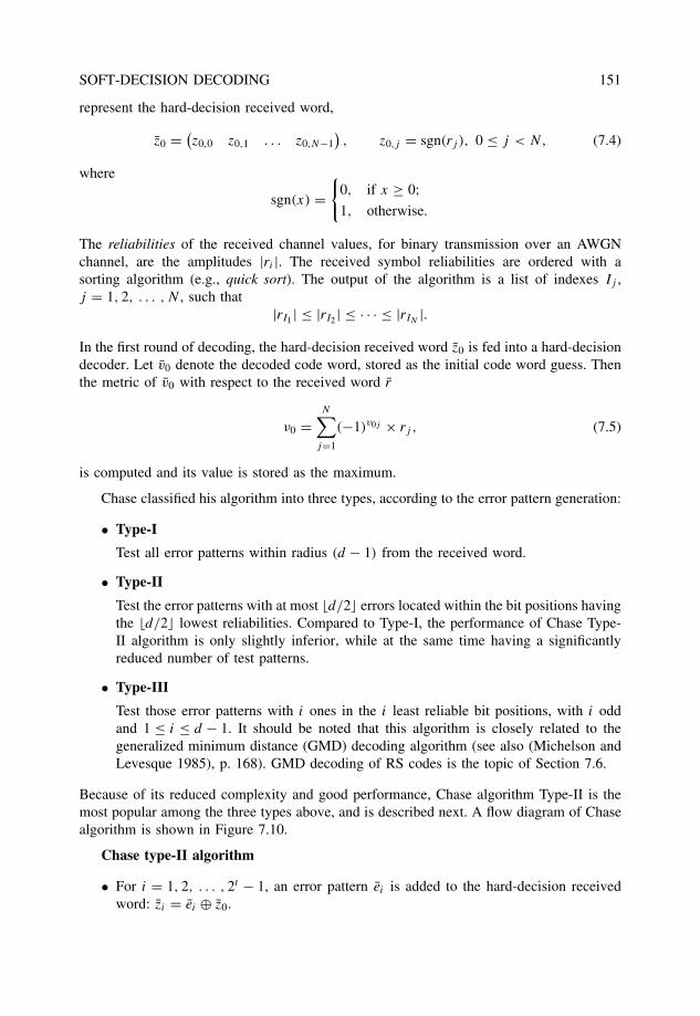
SOFT-DECISION DECODING 151
represent the hard-decision received word,
z0 = (z0,0 z0,1 . . . z0,N−1
), z0,j = sgn(rj ), 0 ≤ j < N, (7.4)
where
sgn(x) ={
0, if x ≥ 0;1, otherwise.
The reliabilities of the received channel values, for binary transmission over an AWGNchannel, are the amplitudes |ri |. The received symbol reliabilities are ordered with asorting algorithm (e.g., quick sort). The output of the algorithm is a list of indexes Ij ,j = 1, 2, . . . , N , such that
|rI1 | ≤ |rI2 | ≤ · · · ≤ |rIN |.
In the first round of decoding, the hard-decision received word z0 is fed into a hard-decisiondecoder. Let v0 denote the decoded code word, stored as the initial code word guess. Thenthe metric of v0 with respect to the received word r
ν0 =N∑
j=1
(−1)v0j × rj , (7.5)
is computed and its value is stored as the maximum.
Chase classified his algorithm into three types, according to the error pattern generation:
• Type-I
Test all error patterns within radius (d − 1) from the received word.
• Type-II
Test the error patterns with at most �d/2� errors located within the bit positions havingthe �d/2� lowest reliabilities. Compared to Type-I, the performance of Chase Type-II algorithm is only slightly inferior, while at the same time having a significantlyreduced number of test patterns.
• Type-III
Test those error patterns with i ones in the i least reliable bit positions, with i oddand 1 ≤ i ≤ d − 1. It should be noted that this algorithm is closely related to thegeneralized minimum distance (GMD) decoding algorithm (see also (Michelson andLevesque 1985), p. 168). GMD decoding of RS codes is the topic of Section 7.6.
Because of its reduced complexity and good performance, Chase algorithm Type-II is themost popular among the three types above, and is described next. A flow diagram of Chasealgorithm is shown in Figure 7.10.
Chase type-II algorithm
• For i = 1, 2, . . . , 2t − 1, an error pattern ei is added to the hard-decision receivedword: zi = ei ⊕ z0.
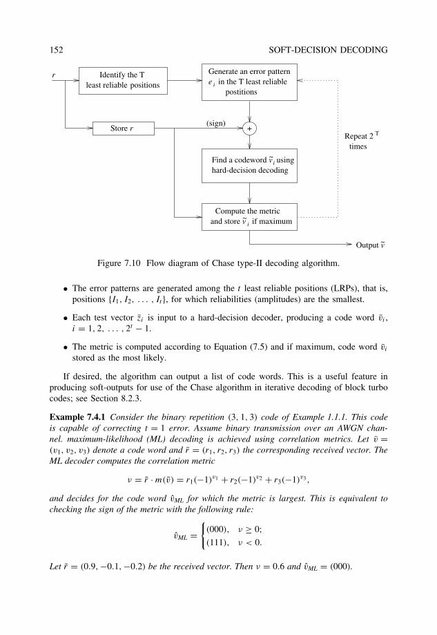
152 SOFT-DECISION DECODING
i
i
i
rleast reliable positions
Identify the T Generate an error patterne in the T least reliable
postitions
+
hard-decision decoding
~
Compute the metric and store v if maximum
Store rRepeat 2
times
T
Output v~
~
(sign)
Find a codeword v using
Figure 7.10 Flow diagram of Chase type-II decoding algorithm.
• The error patterns are generated among the t least reliable positions (LRPs), that is,positions {I1, I2, . . . , It }, for which reliabilities (amplitudes) are the smallest.
• Each test vector zi is input to a hard-decision decoder, producing a code word vi ,i = 1, 2, . . . , 2t − 1.
• The metric is computed according to Equation (7.5) and if maximum, code word vi
stored as the most likely.
If desired, the algorithm can output a list of code words. This is a useful feature inproducing soft-outputs for use of the Chase algorithm in iterative decoding of block turbocodes; see Section 8.2.3.
Example 7.4.1 Consider the binary repetition (3, 1, 3) code of Example 1.1.1. This codeis capable of correcting t = 1 error. Assume binary transmission over an AWGN chan-nel. maximum-likelihood (ML) decoding is achieved using correlation metrics. Let v =(v1, v2, v3) denote a code word and r = (r1, r2, r3) the corresponding received vector. TheML decoder computes the correlation metric
ν = r · m(v) = r1(−1)v1 + r2(−1)v2 + r3(−1)v3,
and decides for the code word vML for which the metric is largest. This is equivalent tochecking the sign of the metric with the following rule:
vML ={
(000), ν ≥ 0;(111), ν < 0.
Let r = (0.9, −0.1, −0.2) be the received vector. Then ν = 0.6 and vML = (000).
SOFT-DECISION DECODING 153
Using Chase type-II algorithm, the hard-decision received word is
z0 = sgn(r) = (011),
which is decoded as v0 = (111). This is the initial code word guess, which is stored togetherwith the metric
ν0 = −r1 − r2 − r3 = −0.9 + 0.1 + 0.2 = −0.6
The reliabilities of the received values are sorted, resulting in |r2| < |r3| < |r1|. There-fore, the second position is the least reliable. The number of error patterns here is 2t =1 : {(010)}, i.e., one error in the second position. This results in
z1 = z0 ⊕ (010) = (001),
which is decoded as v1 = (000), with metric
ν1 = r1 + r2 + r3 = 0.6.
Since ν1 > ν0, the decoder decides that v = v1 = (000) is the most likely code word. In thiscase, the Chase type-II algorithm finds the ML code word successfully.
7.5 Ordered statistics decoding
The ordered statistics decoding (OSD) algorithm (Fossorier and Lin 1995) is similar to theChase algorithm in the sense of creating a list of error patterns and using hard-decisiondecoding. However, unlike the algorithm in the previous section, which deals with leastreliable code positions, OSD considers a list of code words drawn from a set of (permuted)most reliable information positions.
Assume that an (N, K) linear block code C, with generator matrix G and minimumdistance dH ≥ 2t + 1, is used with binary transmission over an AWGN channel. Let
c = (c1, c2, . . . , cN)
denote a code word of C, and let
r = (r1, r2, . . . , rN)
be the received sequence.As in the Chase algorithm above, the decoding process begins by reordering the com-
ponents of the received sequence in decreasing order of reliability value. Let
y = (y1, y2, . . . , yN)
denote the resulting sequence, where |y1| ≥ |y2| ≥ · · · ≥ |yN |. This reordering defines apermutation mapping λ1 such that y = λ1 [r] .
The next step is to permute the columns of G using λ1:
G′ = λ1 [G] = (g′
1 g′2 . . . g′
N
),
where g′j denotes the j -th column of G′.
154 SOFT-DECISION DECODING
A most reliable basis is obtained in the next step of the algorithm as follows:Starting from the first column of G′, find the first K linearly independent (LI) columns
with the largest associated reliability values. Then, these K LI columns are used as thefirst K columns of a new matrix G′′, maintaining their reliability order. The remaining(N − K) columns of G′′ are also arranged in decreasing reliability order. This processdefines a second permutation mapping λ2, such that
G′′ = λ2[G′] = λ2 [λ1 [G]] .
Applying the map λ2 to y results in the reordered received sequence:
z = λ2[y] = (z1, z2, . . . , zk, zk+1, . . . , zN),
with |z1| ≥ |z2| ≥ · · · ≥ |zK | and |zk+1| ≥ · · · ≥ |zN |. By performing elementary row oper-ations on G′′, a systematic form G1 can be obtained:
G1 = (Ik P
) =
1 0 · · · 0 p1,1 · · · p1,N−K
0 1 · · · 0 p2,1 · · · p2,N−K
......
. . ....
.... . .
...
0 0 · · · 1 pk,1 · · · pk,N−K
.
It is easy to see that the code generated by G1 is equivalent to G, in the sense that thesame code words are generated, with permuted code bit positions.
The next step is to perform HDD based on the k most reliable (MR) values of thepermuted received sequence z. Let ua = (u1, u2, . . . , uK) denote the result. Then, thecorresponding code word in C1 can be computed as
v = uaG1 = (v0 v1 . . . vK−1 vK . . . vN
).
The estimated code word vHD in C can be obtained from v, via the inverse mappingλ−1
1 λ−12 , as
vHD = λ−11
[λ−1
2 [v]]. (7.6)
On the basis of the hard-decision–decoded code word v, the algorithm proceeds to reprocessit until either practically optimum or a predefined desired error performance is achieved.
Order-� reprocessing
For 1 ≤ i ≤ �, make all possible changes of i of the k MR bits of v.
For each change, find the corresponding code word v′ in C1 and map it onto a binaryreal sequence x ′, via the mapping {0, 1} → {+1, −1}.For each candidate code word generated, compute the squared Euclidean distance3
between the generated sequence x ′ and the reordered received sequence z. After allthe
∑�i=0
(K
i
)code words have been generated and their distances compared, the
algorithm outputs the code word v∗ which is closest to z.
From v∗, using the inverse map (7.6), the most likely code sequence v∗ML is computed.
3See equation (1.35) of Chapter 1.
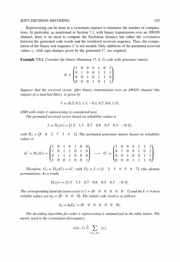
SOFT-DECISION DECODING 155
Reprocessing can be done in a systematic manner to minimize the number of computa-tions. In particular, as mentioned in Section 7.1, with binary transmission over an AWGNchannel, there is no need to compute the Euclidean distance but rather the correlationbetween the generated code words and the reordered received sequence. Thus, the compu-tation of the binary real sequence x ′ is not needed. Only additions of the permuted receivedvalues zi , with sign changes given by the generated v∗, are required.
Example 7.5.1 Consider the binary Hamming (7, 4, 3) code with generator matrix
G =
1 0 0 0 1 0 10 1 0 0 1 1 10 0 1 0 1 1 00 0 0 1 0 1 1
.
Suppose that the received vector, after binary transmission over an AWGN channel (theoutputs of a matched filter), is given by
r = (0.5, 0.3, 1.3, −0.1, 0.7, 0.6, 1.5).
OSD with order-1 reprocessing is considered next.The permuted received vector based on reliability values is
y = �1(r) = (1.5 1.3 0.7 0.6 0.5 0.3 −0.1
),
with �1 = (5 6 2 7 3 4 1
). The permuted generator matrix based on reliability
values is
G′ = �1(G) =
1 0 1 0 1 0 01 0 1 1 0 1 00 1 1 1 0 0 01 0 0 1 0 0 1
−→ G′ =
1 0 0 0 1 1 10 1 0 0 1 0 10 0 1 0 0 1 10 0 0 1 1 1 0
.
Therefore, G1 = �2(G′) = G′, with �2 = I = (
1 2 3 4 5 6 7)
(the identitypermutation). As a result,
�2(y) = (1.5 1.3 0.7 0.6 0.5 0.3 −0.1
).
The corresponding hard-decision vector is z = (0 0 0 0 0 0 1
)and the k = 4 most
reliable values are u0 = (0 0 0 0
). The initial code word is as follows:
v0 = u0G1 = (0 0 0 0 0 0 0
).
The decoding algorithm for order-1 reprocessing is summarized in the table below. Themetric used is the correlation discrepancy:
λ(v�, z)�=
∑i:v�,i �=zi
|yi |.
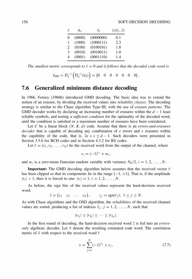
156 SOFT-DECISION DECODING
� u� v� λ(v�, z)
0 (0000) (0000000) 0.11 (1000) (1000111) 2.32 (0100) (0100101) 1.83 (0010) (0010011) 1.04 (0001) (0001110) 1.4
The smallest metric corresponds to � = 0 and it follows that the decoded code word is
vHD = �−11
(�−1
2 (v0))
= (0 0 0 0 0 0 0
).
7.6 Generalized minimum distance decoding
In 1966, Forney (1966b) introduced GMD decoding. The basic idea was to extend thenotion of an erasure, by dividing the received values into reliability classes. The decodingstrategy is similar to the Chase algorithm Type-III, with the use of erasure patterns. TheGMD decoder works by declaring an increasing number of erasures within the d − 1 leastreliable symbols, and testing a sufficient condition for the optimality of the decoded word,until the condition is satisfied or a maximum number of erasures have been considered.
Let C be a linear block (N, K, d) code. Assume that there is an errors-and-erasuresdecoder that is capable of decoding any combination of e errors and s erasures withinthe capability of the code, that is, 2e + s ≤ d − 1. Such decoders were presented inSection 3.5.6 for BCH codes and in Section 4.3.2 for RS codes.
Let r = (r1, r2, . . . , rN) be the received word from the output of the channel, where
ri = (−1)ci + wi,
and wi is a zero-mean Gaussian random variable with variance N0/2, i = 1, 2, . . . , N .
Important: The GMD decoding algorithm below assumes that the received vector r
has been clipped so that its components lie in the range [−1, +1]. That is, if the amplitude|ri | > 1, then it is forced to one: |ri | = 1, i = 1, 2, . . . , N .
As before, the sign bits of the received values represent the hard-decision receivedword,
z = (z1 z2 . . . zN
), zj = sgn(rj ), 1 ≤ j ≤ N.
As with Chase algorithms and the OSD algorithm, the reliabilities of the received channelvalues are sorted, producing a list of indexes Ij , j = 1, 2, . . . , N , such that
|rI1 | ≤ |rI2 | ≤ · · · ≤ |rIN |.In the first round of decoding, the hard-decision received word z is fed into an errors-
only algebraic decoder. Let v denote the resulting estimated code word. The correlationmetric of v with respect to the received word r
ν =N∑
j=1
(−1)vj × rj , (7.7)
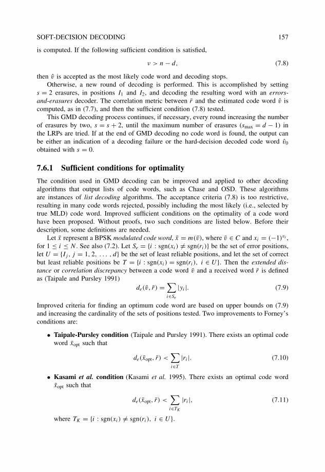
SOFT-DECISION DECODING 157
is computed. If the following sufficient condition is satisfied,
ν > n − d, (7.8)
then v is accepted as the most likely code word and decoding stops.Otherwise, a new round of decoding is performed. This is accomplished by setting
s = 2 erasures, in positions I1 and I2, and decoding the resulting word with an errors-and-erasures decoder. The correlation metric between r and the estimated code word v iscomputed, as in (7.7), and then the sufficient condition (7.8) tested.
This GMD decoding process continues, if necessary, every round increasing the numberof erasures by two, s = s + 2, until the maximum number of erasures (smax = d − 1) inthe LRPs are tried. If at the end of GMD decoding no code word is found, the output canbe either an indication of a decoding failure or the hard-decision decoded code word v0
obtained with s = 0.
7.6.1 Sufficient conditions for optimality
The condition used in GMD decoding can be improved and applied to other decodingalgorithms that output lists of code words, such as Chase and OSD. These algorithmsare instances of list decoding algorithms. The acceptance criteria (7.8) is too restrictive,resulting in many code words rejected, possibly including the most likely (i.e., selected bytrue MLD) code word. Improved sufficient conditions on the optimality of a code wordhave been proposed. Without proofs, two such conditions are listed below. Before theirdescription, some definitions are needed.
Let x represent a BPSK modulated code word, x = m(v), where v ∈ C and xi = (−1)vi ,for 1 ≤ i ≤ N . See also (7.2). Let Se = {i : sgn(xi) �= sgn(ri)} be the set of error positions,let U = {Ij , j = 1, 2, . . . , d} be the set of least reliable positions, and let the set of correctbut least reliable positions be T = {i : sgn(xi) = sgn(ri), i ∈ U}. Then the extended dis-tance or correlation discrepancy between a code word v and a received word r is definedas (Taipale and Pursley 1991)
de(v, r) =∑i∈Se
|yi |. (7.9)
Improved criteria for finding an optimum code word are based on upper bounds on (7.9)and increasing the cardinality of the sets of positions tested. Two improvements to Forney’sconditions are:
• Taipale-Pursley condition (Taipale and Pursley 1991). There exists an optimal codeword xopt such that
de(xopt, r) <∑i∈T
|ri |. (7.10)
• Kasami et al. condition (Kasami et al. 1995). There exists an optimal code wordxopt such that
de(xopt, r) <∑i∈TK
|ri |, (7.11)
where TK = {i : sgn(xi) �= sgn(ri), i ∈ U}.
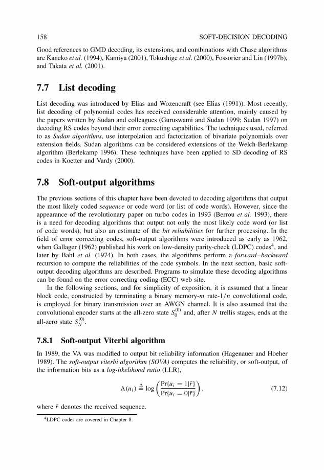
158 SOFT-DECISION DECODING
Good references to GMD decoding, its extensions, and combinations with Chase algorithmsare Kaneko et al. (1994), Kamiya (2001), Tokushige et al. (2000), Fossorier and Lin (1997b),and Takata et al. (2001).
7.7 List decoding
List decoding was introduced by Elias and Wozencraft (see Elias (1991)). Most recently,list decoding of polynomial codes has received considerable attention, mainly caused bythe papers written by Sudan and colleagues (Guruswami and Sudan 1999; Sudan 1997) ondecoding RS codes beyond their error correcting capabilities. The techniques used, referredto as Sudan algorithms, use interpolation and factorization of bivariate polynomials overextension fields. Sudan algorithms can be considered extensions of the Welch-Berlekampalgorithm (Berlekamp 1996). These techniques have been applied to SD decoding of RScodes in Koetter and Vardy (2000).
7.8 Soft-output algorithms
The previous sections of this chapter have been devoted to decoding algorithms that outputthe most likely coded sequence or code word (or list of code words). However, since theappearance of the revolutionary paper on turbo codes in 1993 (Berrou et al. 1993), thereis a need for decoding algorithms that output not only the most likely code word (or listof code words), but also an estimate of the bit reliabilities for further processing. In thefield of error correcting codes, soft-output algorithms were introduced as early as 1962,when Gallager (1962) published his work on low-density parity-check (LDPC) codes4, andlater by Bahl et al. (1974). In both cases, the algorithms perform a forward–backwardrecursion to compute the reliabilities of the code symbols. In the next section, basic soft-output decoding algorithms are described. Programs to simulate these decoding algorithmscan be found on the error correcting coding (ECC) web site.
In the following sections, and for simplicity of exposition, it is assumed that a linearblock code, constructed by terminating a binary memory-m rate-1/n convolutional code,is employed for binary transmission over an AWGN channel. It is also assumed that theconvolutional encoder starts at the all-zero state S
(0)0 and, after N trellis stages, ends at the
all-zero state S(0)N .
7.8.1 Soft-output Viterbi algorithm
In 1989, the VA was modified to output bit reliability information (Hagenauer and Hoeher1989). The soft-output viterbi algorithm (SOVA) computes the reliability, or soft-output, ofthe information bits as a log-likelihood ratio (LLR),
�(ui)�= log
(Pr{ui = 1|r}Pr{ui = 0|r}
), (7.12)
where r denotes the received sequence.
4LDPC codes are covered in Chapter 8.
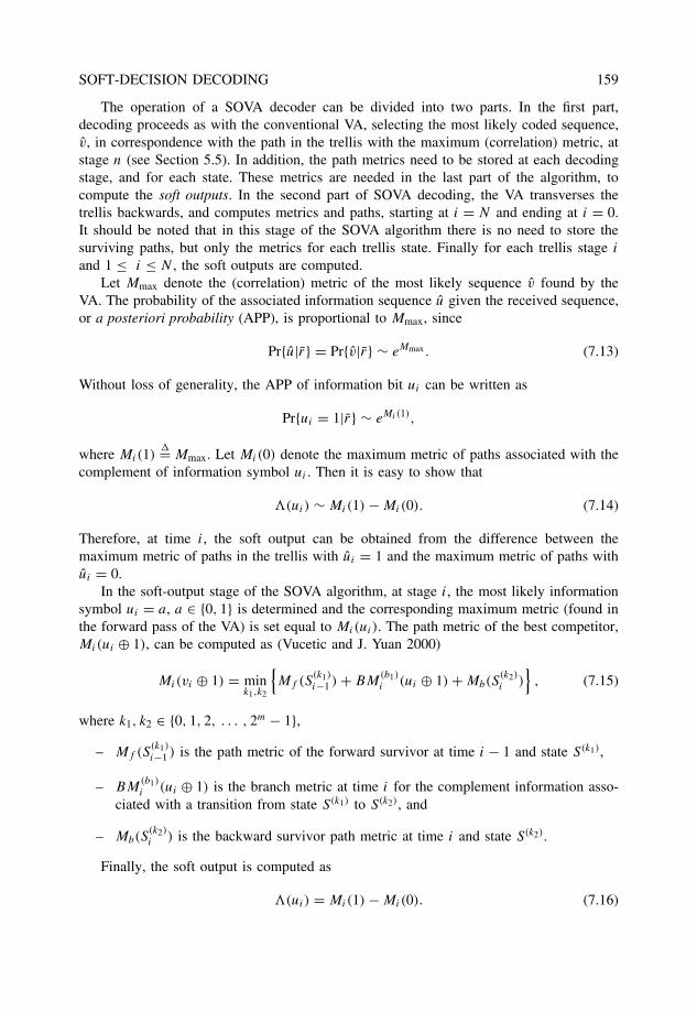
SOFT-DECISION DECODING 159
The operation of a SOVA decoder can be divided into two parts. In the first part,decoding proceeds as with the conventional VA, selecting the most likely coded sequence,v, in correspondence with the path in the trellis with the maximum (correlation) metric, atstage n (see Section 5.5). In addition, the path metrics need to be stored at each decodingstage, and for each state. These metrics are needed in the last part of the algorithm, tocompute the soft outputs. In the second part of SOVA decoding, the VA transverses thetrellis backwards, and computes metrics and paths, starting at i = N and ending at i = 0.It should be noted that in this stage of the SOVA algorithm there is no need to store thesurviving paths, but only the metrics for each trellis state. Finally for each trellis stage i
and 1 ≤ i ≤ N , the soft outputs are computed.Let Mmax denote the (correlation) metric of the most likely sequence v found by the
VA. The probability of the associated information sequence u given the received sequence,or a posteriori probability (APP), is proportional to Mmax, since
Pr{u|r} = Pr{v|r} ∼ eMmax . (7.13)
Without loss of generality, the APP of information bit ui can be written as
Pr{ui = 1|r} ∼ eMi(1),
where Mi(1)�= Mmax. Let Mi(0) denote the maximum metric of paths associated with the
complement of information symbol ui . Then it is easy to show that
�(ui) ∼ Mi(1) − Mi(0). (7.14)
Therefore, at time i, the soft output can be obtained from the difference between themaximum metric of paths in the trellis with ui = 1 and the maximum metric of paths withui = 0.
In the soft-output stage of the SOVA algorithm, at stage i, the most likely informationsymbol ui = a, a ∈ {0, 1} is determined and the corresponding maximum metric (found inthe forward pass of the VA) is set equal to Mi(ui). The path metric of the best competitor,Mi(ui ⊕ 1), can be computed as (Vucetic and J. Yuan 2000)
Mi(vi ⊕ 1) = mink1,k2
{Mf (S
(k1)
i−1 ) + BM(b1)
i (ui ⊕ 1) + Mb(S(k2)
i )}
, (7.15)
where k1, k2 ∈ {0, 1, 2, . . . , 2m − 1},– Mf (S
(k1)
i−1 ) is the path metric of the forward survivor at time i − 1 and state S(k1),
– BM(b1)i (ui ⊕ 1) is the branch metric at time i for the complement information asso-
ciated with a transition from state S(k1) to S(k2), and
– Mb(S(k2)
i ) is the backward survivor path metric at time i and state S(k2).
Finally, the soft output is computed as
�(ui) = Mi(1) − Mi(0). (7.16)
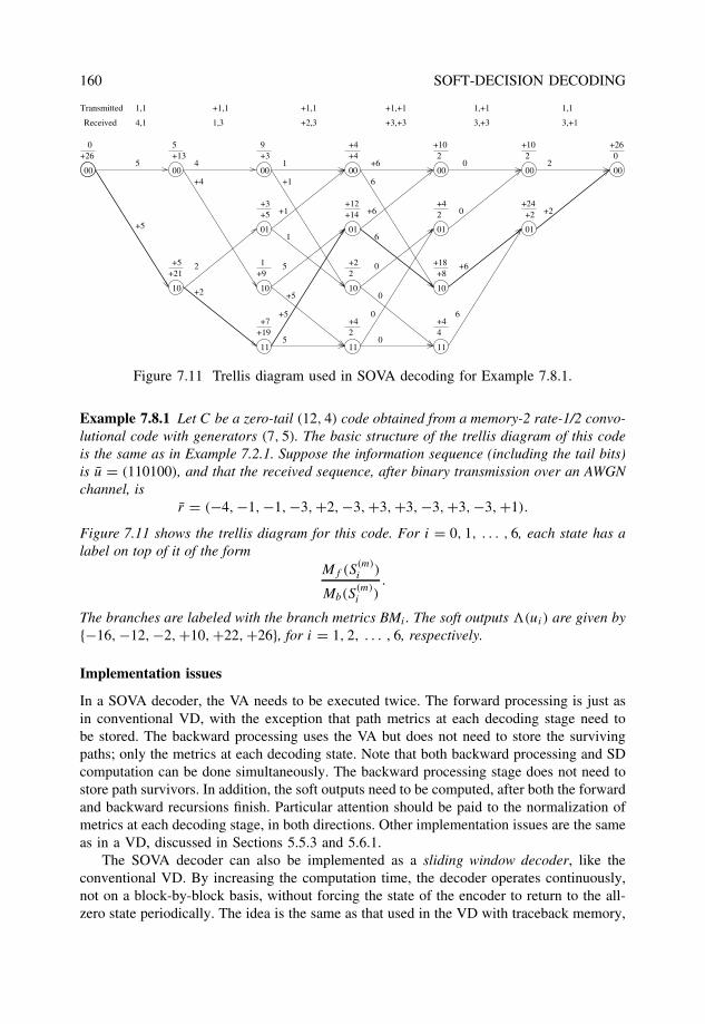
160 SOFT-DECISION DECODING
Transmitted
00 00
10
00
10
11
01
00
10
11
01
00
10
11
01
00
01
005
+5
2
+2
+1
+1
1
+5
5
5
+5
6
6
+6
0
0
0
0
+4
4 1 +6 0
+6
6
2
+20
+260
+21
+14
+19
5+13
+5
+39
+3+5
+91
+7
+4+4
+12
2+2
2+4
+102
+42
+18+8
4+4
+102
+2+24
0+26
4,1 1,3 +2,3 +3,+3 3,+3 3,+1
1,1 +1,1 +1,1 +1,+1 1,+1 1,1
Received
Figure 7.11 Trellis diagram used in SOVA decoding for Example 7.8.1.
Example 7.8.1 Let C be a zero-tail (12, 4) code obtained from a memory-2 rate-1/2 convo-lutional code with generators (7, 5). The basic structure of the trellis diagram of this codeis the same as in Example 7.2.1. Suppose the information sequence (including the tail bits)is u = (110100), and that the received sequence, after binary transmission over an AWGNchannel, is
r = (−4, −1, −1, −3, +2, −3, +3, +3, −3, +3, −3, +1).
Figure 7.11 shows the trellis diagram for this code. For i = 0, 1, . . . , 6, each state has alabel on top of it of the form
Mf (S(m)i )
Mb(S(m)i )
.
The branches are labeled with the branch metrics BMi . The soft outputs �(ui) are given by{−16, −12, −2, +10, +22, +26}, for i = 1, 2, . . . , 6, respectively.
Implementation issues
In a SOVA decoder, the VA needs to be executed twice. The forward processing is just asin conventional VD, with the exception that path metrics at each decoding stage need tobe stored. The backward processing uses the VA but does not need to store the survivingpaths; only the metrics at each decoding state. Note that both backward processing and SDcomputation can be done simultaneously. The backward processing stage does not need tostore path survivors. In addition, the soft outputs need to be computed, after both the forwardand backward recursions finish. Particular attention should be paid to the normalization ofmetrics at each decoding stage, in both directions. Other implementation issues are the sameas in a VD, discussed in Sections 5.5.3 and 5.6.1.
The SOVA decoder can also be implemented as a sliding window decoder, like theconventional VD. By increasing the computation time, the decoder operates continuously,not on a block-by-block basis, without forcing the state of the encoder to return to the all-zero state periodically. The idea is the same as that used in the VD with traceback memory,
SOFT-DECISION DECODING 161
as discussed in Section 5.5.3, where forward recursion, traceback and backward recursion,and soft-output computations are implemented in several memory blocks (see also (Viterbi1998)).
7.8.2 Maximum-a posteriori (MAP) algorithm
The Bahl-Cocke-Jelinek-Raviv (BCJR) algorithm (Bahl et al. 1974) is an optimal symbol-by-symbol MAP decoding method for linear block codes that minimizes the probability ofa symbol error. The goal of this MAP decoder is to examine the received sequence r and tocompute the a posteriori probabilities of the input information bits, as in (7.12). The MAPalgorithm is described next, following closely the arguments in Bahl et al. (1974).
The state transitions (or branches) in the trellis have probabilities
Pr{S
(m)i |S(m′)
i−1
}, (7.17)
and for the output symbols vi ,
qi(xi |m′, m)�= Pr
{xi = x|S(m′)
i−1 , S(m)i
}, (7.18)
where x = ±1, and xi = m(vi) = (−1)vi , 0 < i ≤ N .The sequence x is transmitted over an AWGN channel and received as a sequence r ,
with transition probabilities
Pr {r|x} =N∏
i=1
p(ri |xi ) =N∏
i=1
n−1∏j=0
p(ri,j |xi,j ), (7.19)
where p(ri,j |xi,j ) is given by (7.1).
Let B(j)
i be the set of branches connecting state S(m′)i−1 to state S
(m)i such that the asso-
ciated information bit ui = j , with j ∈ {0, 1}. Then
Pr {ui = j |r} =∑
(m′,m)∈B(j)i
Pr{S
(m′)i−1 , S
(m)i , r
}�=
∑(m′,m)∈B
(j)i
σi(m′, m). (7.20)
The value of σi(m′, m) in (7.20) is equal to
σi(m′, m) = αi−1(m
′) · γ(j)
i (m′, m) · βi(m), (7.21)
where the joint probability αi(m)�= Pr
{S
(m)i , rp
}is given recursively by
αi(m) =∑m′
αi−1(m′) ·
1∑j=0
γ(j)
i (m′, m), (7.22)
and is referred to as the forward metric.
The conditional probability γ(j)
i (m′, m)�= Pr
{S
(m)i , r|S(m′)
i−1
}is given by
γ(j)
i (m′, m) =∑
x
pi(m|m′)Pr{xi = x|S(m′)
i−1 , S(m)i
}· Pr {ri |x} (7.23)
162 SOFT-DECISION DECODING
where pi(m|m′) = Pr{S
(m)i |S(m′)
i−1
}, which for the AWGN channel can be put in the form
γ(j)
i (m′, m) = Pr {ui = j} · δij (m, m′) · exp
− 1
N0
n−1∑q=0
(ri,q − xi,q)2
, (7.24)
where δij (m, m′) = 1 if {m′, m} ∈ B(j)
i , and δij (m, m′) = 0 otherwise. γ(j)
i (m′, m) isreferred to as the branch metric.
The conditional probability βi(m)�= Pr
{rf |S(m)
i
}is given by
βi(m) =∑m′
βi+1(m′) ·
1∑j=0
γ(j)
i (m′, m), (7.25)
and referred to as the backward metric.Combining (7.25), (7.24), (7.22) , (7.21) and (7.12), the soft output (LLR) of information
bit ui is given by
�(ui) = log
(Pr{ui = 1|r}Pr{ui = 0|r}
)= log
∑m
∑m′
αi−1(m′)γ (1)
i (m′, m)βi(m)
∑m
∑m′
αi−1(m′)γ (0)
i (m′, m)βi(m)
, (7.26)
where the hard-decision output is given by ui = sgn(�(ui)) and the reliability of the bit ui
is |�(ui)|. The above equations can be interpreted as follows. A bidirectional Viterbi-likealgorithm can be applied, just as in SOVA decoding (previous section). In the forwardrecursion, given the probability of a state transition at time i, the joint probability of thereceived sequence up to time i and the state at time i is evaluated. In the backward recursion,the probability of the received sequence from time i + 1 to time N , given the state at timei is computed. Then the soft output depends on the joint probability of the state transitionand the received symbol at time i.
The MAP algorithm can be summarized as follows:
• Initialization
For m = 0, 1, . . . , 2m − 1,
α0(0) = 1, α0(m) = 0, m �= 0,
For m′ = 0, 1, . . . , 2m − 1,
βN(0) = 1, βN(m′) = 0, m′ �= 0,
• Forward recursion
For i = 1, 2, . . . , N ,
1. For j = 0, 1, compute and store the branch metrics γ(j)
i (m′, m) as in (7.24).
2. For m = 0, 1, . . . , 2m − 1, compute and store the forward metrics αi(m) as in(7.22).
SOFT-DECISION DECODING 163
• Backward recursion
For i = N − 1, N − 2, . . . , 0,
1. Compute the backward metrics βi(m) as in (7.25), using the branch metriccomputed in the forward recursion.
2. Compute the LLR �(ui) as in (7.26).
Implementation issues
The implementation of a MAP decoder is similar to that of a SOVA decoder, as bothdecoders perform forward and backward recursions. All the issues mentioned in the previoussection apply to a MAP decoder. In addition, note that branch metrics depend on thenoise power density N0, which should be estimated to keep optimality. To avoid numericalinstabilities, the probabilities αi(m) and βi(m) need to be scaled at every decoding stage,such that
∑m αi(m) = ∑
m βi(m) = 1.
7.8.3 Log-MAP algorithm
To reduce the computational complexity of the MAP algorithm, the logarithms of the metricsmay be used. This results in the so-called log-MAP algorithm.
From (7.22) and (7.25) (Robertson et al. 1995),
log αi(m) = log
∑
m′
1∑j=0
exp(
log αi−1(m′) + log γ
(j)
i (m′, m)) ,
log βi(m) = log
∑
m′
1∑j=0
exp(
log βi+1(m′) + log γ
(j)
i (m′, m)) . (7.27)
Taking the logarithm of γ(j)
i (m′, m) in (7.24),
log γ(j)
i (m′, m) = δij (m, m′)
log Pr {ui = j} − 1
N0
n−1∑q=0
(ri,q − xi,q)2
(7.28)
By defining αi(m) = log αi(m), βi(m) = log βi(m) and γ(j)
i (m′, m) = log γ(j)
i (m′, m),(7.26) can be written as
�(ui) = log
∑m
∑m′
exp(αi−1(m
′) + γ(0)i (m′, m) + βi (m)
)∑m
∑m′
exp(αi−1(m
′) + γ(1)i (m′, m) + βi (m)
) , (7.29)
and an algorithm that works in the log-domain is obtained.The following expression, known as the Jacobian logarithm (Robertson et al. 1995), is
used to avoid the sum of exponential terms,
log(eδ1 + eδ2
) = max (δ1, δ2) + log(1 + e−|δ1−δ2|) , (7.30)
164 SOFT-DECISION DECODING
The function log(1 + e−|δ1−δ2|) can be stored in a small look-up table (LUT), as only a
few values (eight reported in Robertson et al. (1995)) are required to achieve practicallythe same performance as the MAP algorithm. Therefore, instead of several calls to slow(or hardware-expensive) exp(x) functions, simple LUT accesses give practically the sameresult.
7.8.4 Max-Log-MAP algorithm
A more computationally efficient, albeit suboptimal derivative of the MAP algorithm is theMax-Log-MAP algorithm. It is obtained as before, by taking the logarithms of the MAPmetrics and using the approximation (Robertson et al. 1995)
log(eδ1 + eδ2
) ≈ max (δ1, δ2) , (7.31)
which is equal to the first term on the right-hand side of (7.30). As a result, the LLR ofinformation bit ui is given by
�(ui) ≈ maxm′,m
{αi−1(m
′) + γ(0)i (m′, m) + βi (m)
}− max
m′,m
{αi−1(m
′) + γ(1)i (m′, m) + βi(m)
}. (7.32)
The forward and backward computations can now be expressed as
αi(m) = maxm′ max
j∈{0,1}
{αi−1(m
′) + γ(j)
i (m′, m)}
,
βi(m) = maxm′ max
j∈{0,1}
{βi+1(m
′) + γ(j)
i (m′, m)}
. (7.33)
For binary codes based on rate-1/n convolutional encoders, in terms of decoding complexity(measured in number of additions and multiplications), the SOVA algorithm requires theleast amount, about half of that of the max-log-MAP algorithm. The log-MAP algorithmis approximately twice as complex compared to the max-log-MAP algorithm. In terms ofperformance, it has been shown (Fossorier et al. 1998) that the max-log-MAP algorithmis equivalent to a modified SOVA algorithm. The log-MAP and MAP algorithms have thesame best error performance.
7.8.5 Soft-output OSD algorithm
The OSD algorithm of Section 7.5 can be modified to output the symbol reliabili-ties (Fossorier and Lin 1998). This modification is referred to as the soft-output OSD,or SO-OSD. The SO-OSD algorithm is a two-stage order-i reprocessing. The first stage isthe same as conventional OSD, determining the most likely code word vML up to order-ireprocessing. To describe the second stage, the following definitions are required.
For each most reliable position j , 1 ≤ j ≤ K , define the code word vML(j) obtainedby complementing position j in vML,
vML(j) = vML ⊕ e(j),
SOFT-DECISION DECODING 165
where e(j) is the set of all length-K vectors of Hamming weight one. The vector e(j) isthe coset representative of the partition of code C1 (equivalent to the original code afterreordering, as in OSD, see Section 7.5) into two sets of code words, having the j -th positionequal to zero, or one in code words of C. These sets, after removing position j , becomepunctured subcodes of C1, and are denoted C(0) and C(1). Let C(j) = C(0).
The SO-OSD algorithm consists of the following steps:
1. Determine the most likely code word vML covered by order-i reprocessing.
2. For each subcode C(j), 1 ≤ j ≤ K ,
(a) Initialize all soft output values of the LRPs based on vML and vML(j). That is,compute
Lj = rj +∑� �=j
v�(0) �=v�(1)
m(v�(1))r�, (7.34)
where m(vi) = (−1)vi .
(b) Determine the most likely code word v(j) ∈ C(j) covered by order-i repro-cessing.
(c) Evaluate Lj (7.34) on the basis of vML and v(j).
(d) Update soft output values of LRP in the positions of vML ⊕ v(j) with Lj .
3. For K + 1 ≤ j ≤ N , choose the smallest output value associated with each LRP j .
The performance of SO-OSD is the same as max-log-MAP decoding for many binary linearblock codes of length up to 128 and high-rate codes (Fossorier and Lin 1998). In addition,scaling down the extrinsic values (7.34) improves the performance by a few tenths of a dB.
Problems
1. Let C be the binary memory-2 convolutional encoder with generators (7, 5).
(a) Simulate the performance of C over an AWGN channel with BPSK modulationand SD Viterbi decoding.
(b) Use the bounds for hard- (HD) and soft-decision (SD) decoding and comparethem with your simulations. What is the difference between required Eb/N0
(dB) between HD and SD in order to achieve a probability of error Pe ≈ 10−4?
2. Repeat Problem 1 for the binary memory-2 recursive systematic convolutional (RSC)encoder with generators (1, 5/7).
3. Let CO be an RS (7, 5, 3) code over GF(23) and CI be the binary rate-1/2 K = 3 non-systematic convolutional code with generators g = (7, 5). Consider a concatenatedcode CO CI with CO as outer code and CI as inner code, as depicted below:
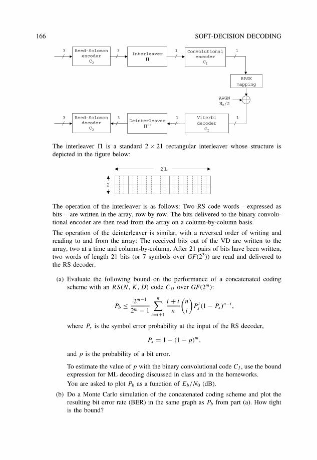
166 SOFT-DECISION DECODING
Reed-Solomonencoder
CO
InterleaverΠ
Convolutionalencoder
CI
BPSKmapping
3 3 1 1
AWGNN0/2
Reed-Solomondecoder
CO
DeinterleaverΠ−1
Viterbidecoder
CI
3 3 1 1
The interleaver � is a standard 2 × 21 rectangular interleaver whose structure isdepicted in the figure below:
21
2
The operation of the interleaver is as follows: Two RS code words – expressed asbits – are written in the array, row by row. The bits delivered to the binary convolu-tional encoder are then read from the array on a column-by-column basis.
The operation of the deinterleaver is similar, with a reversed order of writing andreading to and from the array: The received bits out of the VD are written to thearray, two at a time and column-by-column. After 21 pairs of bits have been written,two words of length 21 bits (or 7 symbols over GF(23)) are read and delivered tothe RS decoder.
(a) Evaluate the following bound on the performance of a concatenated codingscheme with an RS(N, K, D) code CO over GF(2m):
Pb ≤ 2m−1
2m − 1
n∑i=t+1
i + t
n
(n
i
)P i
s (1 − Ps)n−i ,
where Ps is the symbol error probability at the input of the RS decoder,
Ps = 1 − (1 − p)m,
and p is the probability of a bit error.
To estimate the value of p with the binary convolutional code CI , use the boundexpression for ML decoding discussed in class and in the homeworks.
You are asked to plot Pb as a function of Eb/N0 (dB).
(b) Do a Monte Carlo simulation of the concatenated coding scheme and plot theresulting bit error rate (BER) in the same graph as Pb from part (a). How tightis the bound?

SOFT-DECISION DECODING 167
4. Consider the binary repetition (5, 1, 5) code, denoted by C. In this problem youare asked to analyze the performance of C with binary transmission BPSK over anAWGN channel. Write computer programs to accomplish the following tasks:
(a) Simulate the BER performance of ML decoding. (Hint: Look at the sign of the
correlation ν = ∑5i=1 ri , where (r1, r2, r3, r4, r5) is the received vector.)
(b) Simulate the BER performance of Chase type-II algorithm. (Hint: t = 2.)
(c) Plot the results of (a) and (b) together with the union bound.
5. Simulate the performance of SD Viterbi decoding of the binary rate-1/2 convolutionalcodes listed below and compare the plots. On the basis of your simulations, estimatethe increment in coding gain that results from doubling the number of states of theencoder.
Constraint length, K Generators (g0, g1) dfree
4 (15,17) 65 (23,35) 76 (53,75) 87 (133,171) 109 (561,753) 12
6. Let C be a binary Hamming (7, 4) code.
(a) List all the 16 code words of C.
(b) Build a computer model of an ML decoder of C for binary modulation over anAWGN channel. Assume that the mapping is “0” → +1 and “1” → −1. Thedecoder computes a total of 16 metrics, one per code word, and selects the codeword with maximum metric as the ML code word. Simulate the performanceof this ML decoder and compare with that of a hard-decision decoder.
(c) Build a computer model of a soft-decision (SD) decoder of C using the Type-IIChase algorithm. Simulate the performance of this SD decoder and comparewith the ML decoder.
(d) Suppose that the received vector (from the outputs of the matched filter) is
r = (0.8, −0.1, 1.1, −0.2, 0.4, 0.6, 1.5).
Using ordered-statistics decoding with order-1 reprocessing, determine the MLcodeword.
7. Give a geometric interpretation of decoding of the binary repetition (3, 1, 3) codewith Chase type-II algorithm presented in Example 7.4.1.
8. Show that the Chase decoding algorithms (types 1 through 3) and ML decoding havethe same asymptotic behavior. That is, the probability of error decreases exponentiallywith Eb/N0 within a constant factor. (Hint: Section IV of Chase (1972).)
168 SOFT-DECISION DECODING
9. For the convolutional encoder and information sequence in Example 7.8.1, computethe soft outputs using the BCJR algorithm.
10. (Lin and Costello) Consider a memory-1 RSC encoder with generators (1, 1/3). Usingthe zero-tail construction, a binary linear (8, 3) code C is constructed.
(a) What is the minimum distance of C?
(b) Assume that the received sequence is
r = (+0.8, +0.1, +1.0, −0.5, −1.8, +1.1, +1.6, −1.6),
which is normalized with respect to√
Es . Assume also that Es/N0 = 1/4. Usingthe BCJR (MAP) algorithm, determine the most likely information sequence.
8
Iteratively decodable codes
Iterative decoding may be defined as a technique employing a soft-output decoding algo-rithm that is iterated several times to improve the error performance of a coding scheme,with the aim of approaching true maximum-likelihood decoding (MLD) with least com-plexity. When the underlying error correcting code is well designed, increasing the numberof iterations results in an improvement of the error performance.
Iterative decoding techniques date back to 1954 with the work of Elias (1954) oniterated codes. Later, in the 1960s, Gallager (1962) and Massey (1963) made importantcontributions. Iterative decoding in those days was referred to as probabilistic decoding.The main concept was then, as it is today, to maximize the a posteriori probability of asymbol being sent, given a noisy version of the coded sequence.
In this chapter, code constructions that can be iteratively decoded are presented. Else-where in the literature, these coding schemes have been named turbo-like codes. In termsof the application of iterative decoding algorithms, and for the purpose of this chapter, ECCschemes can be broadly classified into two classes:
Product codes
Examples of codes in this class include parallel concatenated codes or turbo codesand serially concatenated codes. They have found applications in third-generation(3G) cellular systems and deep-space communications. Members of this class arealso block product codes, presented in Section 6.2.4.
Low-density parity-check (LDPC) codes
These are linear codes with the property that their parity-check matrix has a smallratio of number of nonzero elements to the total number of elements. LDPC codeshave found applications in second-generation satellite broadcasting systems (DVB-S2), in gigabit ethernet systems (10Gbase-T), and are being considered in high-speedwireless LAN systems (IEEE 802.3an).
In both the above classes of codes, the component codes can be either convolutional or blockcodes, with systematic or nonsystematic encoding, or any combination thereof. To provide
The Art of Error Correcting Coding, Second Edition Robert H. Morelos-Zaragoza 2006 John Wiley & Sons, Ltd. ISBN: 0-470-01558-6
170 ITERATIVELY DECODABLE CODES
a motivation for the study of iterative decoding techniques, the fundamental structure ofturbo codes is discussed next.
Turbo codes
Over the past eight years, there has been an enormous amount of research effort dedicatedto the analysis of iterative decoding algorithms and the construction of iteratively decodablecodes or “turbo-like codes” that approach the Shannon limit.1 Turbo codes were introducedin 1993 (Berrou et al. 1993). The results reported there sent a shock wave throughout theresearch community.
With binary transmission over an AWGN channel, a rate-1/2 coding scheme, based ona combination of two rate-1/2 16-state RSC codes, connected with an interleaver of size256 × 256, achieved BER rates of 10−5 at a signal-to-noise ratio (SNR) per bit, or Eb/N0
of 0.7 dB very close to the Shannon limit (0.2 dB).The basic elements in the turbo coding scheme proposed in Berrou et al. (1993) are the
following:
Coding structure
A two-dimensional product code2 structure with constituent recursive systematic con-volutional encoders.
Reliability-based decoding
Employ soft-input soft-output (SISO) maximum a posteriori (MAP) decoders for thecomponent codes in order to generate log-likelihood ratios.
Iterative decoding
The use of feedback of part of the symbol reliabilities, in the form of extrinsicinformation from an outer (column) decoder to an inner (row) decoder, and viceversa.
Random permutation
A long random interleaver applied between the two encoders. Its main function is toensure that, at each iteration, the component MAP decoders get independent estimateson the information symbols.
These four elements have been extensively studied over the years. References Heegard andWicker 1999; ISTC 1997, 2000; JSAC-I 2001; JSAC-II 2001; Vucetic and J. Yuan 2000continue to be a good sample of the research efforts.
Log-likelihood ratio (LLR) value
In the iterative decoding algorithms presented next, the LLR log-likelihood ratio (LLR)value becomes very important and is defined as
�(u)�= log
(Pr{u = 1}Pr{u = 0}
)= log
(Pr{m(u) = −1}Pr{m(u) = +1}
)= log
(p1
p0
),
1The Shannon limit refers to the capacity of a discrete-input continuous output channel.2A product code is referred to in the original paper (Berrou et al. 1993) as a parallel concatenated code.
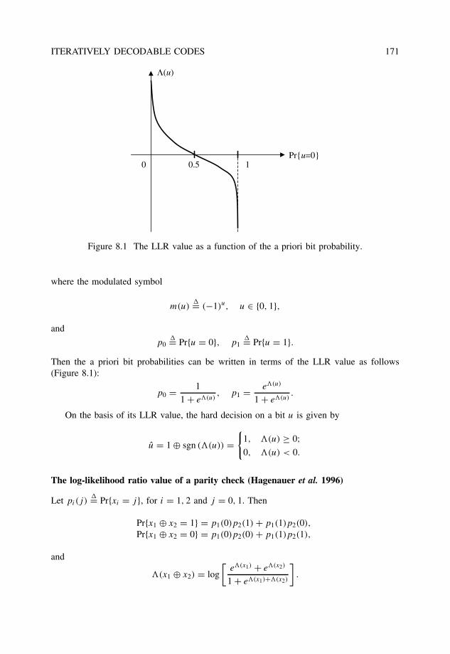
ITERATIVELY DECODABLE CODES 171
Pr{u=0}10.50
Λ(u)
Figure 8.1 The LLR value as a function of the a priori bit probability.
where the modulated symbol
m(u)�= (−1)u, u ∈ {0, 1},
and
p0�= Pr{u = 0}, p1
�= Pr{u = 1}.Then the a priori bit probabilities can be written in terms of the LLR value as follows(Figure 8.1):
p0 = 1
1 + e�(u), p1 = e�(u)
1 + e�(u).
On the basis of its LLR value, the hard decision on a bit u is given by
u = 1 ⊕ sgn (�(u)) ={
1, �(u) ≥ 0;0, �(u) < 0.
The log-likelihood ratio value of a parity check (Hagenauer et al. 1996)
Let pi(j)�= Pr{xi = j}, for i = 1, 2 and j = 0, 1. Then
Pr{x1 ⊕ x2 = 1} = p1(0)p2(1) + p1(1)p2(0),
Pr{x1 ⊕ x2 = 0} = p1(0)p2(0) + p1(1)p2(1),
and
�(x1 ⊕ x2) = log
[e�(x1) + e�(x2)
1 + e�(x1)+�(x2)
].
172 ITERATIVELY DECODABLE CODES
8.1 Iterative decoding
The purpose of this section is to introduce basic concepts behind iterative decoding. Con-sider the a posteriori LLR3 of an information symbol, Equation (7.12) repeated here forconvenience,
�(ui)�= log
(Pr{ui = 1|r}Pr{ui = 0|r}
). (8.1)
Let Ci(0) and Ci(1) denote the set of modulated coded sequences x = m(v) ∈ m(C) suchthat the i-th position in v ∈ C is equal to zero and one, respectively. Recall that modulationwas a one-to-one and onto mapping from v ∈ {0, 1} to x ∈ {+1, −1} as in Equation (7.2).Then the symbol LLR (8.1) can be written as
�(ui) = log
∑x∈Ci(1)
N∏�=1
p(r�, x�)
∑x∈Ci(0)
N∏�=1
p(r�, x�)
= log
p(ri |xi = −1)Pr{xi = −1}∑
x∈Ci(1)
N∏�=1��=i
p(r�, x�)
p(ri |xi = +1)Pr{xi = +1}∑
x∈Ci(0)
N∏�=1��=i
p(r�, x�)
, (8.2)
from which it follows that the LLR of an information symbol can be expressed as
�(ui) = �ci + �a(ui) + �i,e(C), (8.3)
where �ci is known as the channel LLR and given by
�ci = log
(p(ri |xi = −1)
p(ri |xi = +1)
)
=
−(−1)ri log(
1−p
p
), for a BSC channel with parameter p;
− 4
N0ri, for an AWGN channel (σ 2
n = N0/2); and
− 4
N0airi, for a flat Rayleigh fading channel.
(8.4)
�a(ui) = log
(Pr{xi = −1}Pr{xi = +1}
)= log
(Pr{ui = 1}Pr{ui = 0}
)(8.5)
3The LLR is also referred to as “L-value” by some authors.
ITERATIVELY DECODABLE CODES 173
is the a priori LLR of the information bit, and
�i,e(C) = log
∑x∈Ci(1)
N∏�=1��=i
p(r�, x�)
∑x∈Ci(0)
N∏�=1��=i
p(r�, x�)
(8.6)
is the extrinsic LLR, which is specified by the constraints imposed by the code on the otherinformation symbols.
Assume that binary transmission is performed over an AWGN channel and that binaryrate-1/n RSC encoders are used as components. In an iterative decoding procedure, theextrinsic information provided by �i,e(C) can be fed back to the decoder as a prioriprobability for a second round of decoding. In terms of forward–backward decoding usinga trellis (see Section 7.8.2), the extrinsic LLR can be written as
�i,e(C) = log
∑(m,m′)∈Bi(1)
αi−1(m′)ξi(m
′, m)βi(m)
∑(m,m′)∈Bi(0)
αi−1(m′)ξi(m
′, m)βi(m)
, (8.7)
where αi(m) and βi(m) are given by Equations (7.22) and (7.25), respectively.A modified branch metric is needed to compute the extrinsic LLR
ξi(m′, m) = δij (m, m′) exp
E
N0
n−1∑q=1
ri,qxi,q
, (8.8)
where, as before,
δij (m, m′) ={
1, if (m′, m) ∈ B(j)
i
0, otherwise.
This extrinsic LLR, for an information position i, does not contain any variable directlyrelated to ui , for i = 1, 2, . . . , N . It should be noted that because of the assumption thatencoding is systematic, the branch labels in the trellis are of the form (ui, vi,1, . . . , vi,n−1),and therefore the sum in the modified branch metric (8.8) starts at q = 1.4
In the more general case of a two-dimensional product coding scheme, the first (e.g.,row) decoder produces �
(1)i,e (C) which is given to the second (e.g., column) decoder as a
priori probability �(2)a (ui) to be used in the computation of the LLR of information symbol
ui . In other words, the extrinsic information provides a soft output that involves only softinputs (reliabilities) that are not directly related to the information symbol ui . Iterativedecoding of product codes is the topic of the next section.
4Compare this with the expression of the branch metric γ(j)
i (m′,m) in (7.24).
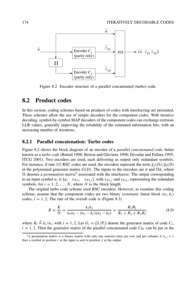
174 ITERATIVELY DECODABLE CODES
u
Πv
P2
vP1
u
(parity only)
(parity only)
P/S )vP2v
P1u(Encoder C
Encoder C
1
2
Figure 8.2 Encoder structure of a parallel concatenated (turbo) code.
8.2 Product codes
In this section, coding schemes based on products of codes with interleaving are presented.These schemes allow the use of simple decoders for the component codes. With iterativedecoding, symbol-by-symbol MAP decoders of the component codes can exchange extrinsicLLR values, generally improving the reliability of the estimated information bits, with anincreasing number of iterations.
8.2.1 Parallel concatenation: Turbo codes
Figure 8.2 shows the block diagram of an encoder of a parallel concatenated code, betterknown as a turbo code (Battail 1998; Berrou and Glavieux 1998; Divsalar and Pollara 1995;ITCG 2001). Two encoders are used, each delivering as output only redundant symbols.For instance, if rate-1/2 RSC codes are used, the encoders represent the term g1(D)/g0(D)
in the polynomial generator matrix G(D). The inputs to the encoders are u and u, where denotes a permutation matrix5 associated with the interleaver. The output correspondingto an input symbol ui is
(ui vP 1,i vP 2,i
), with vP 1,i and vP 2,i representing the redundant
symbols, for i = 1, 2, . . . , N , where N is the block length.The original turbo code scheme used RSC encoders. However, to examine this coding
scheme, assume that the component codes are two binary systematic linear block (ni, ki)
codes, i = 1, 2. The rate of the overall code is (Figure 8.3)
R = K
N= k1k2
n1n2 − (n1 − k1)(n2 − k2)= R1R2
R1 + R2 + R1R2, (8.9)
where Ri�= ki/ni , with i = 1, 2. Let Gi = (
Ii |Pi
)denote the generator matrix of code Ci ,
i = 1, 2. Then the generator matrix of the parallel concatenated code CPC can be put in the
5A permutation matrix is a binary matrix with only one nonzero entry per row and per column; if πi,j = 1then a symbol in position i at the input is sent to position j at the output.
ITERATIVELY DECODABLE CODES 175
following form:
GPC =
Ik1k2
P1
P1
. . .
P1
P2
P2
. . .
P2
= (Ik1k2 | P ′
1 | P ′2
), (8.10)
where is the permutation matrix associated with the interleaver, and Pi is the paritysubmatrix of code Ci , i = 1, 2. The number of times that P1 appears in the middle part P ′
1of GPC is k2, while the number of times that P2 appears in the leftmost portion P ′
2 of GPC
is k1. All other entries in P ′1 and P ′
2 are zero. It follows that codewords of CPC are of theform
(u | uP ′
1 | uP ′2
).
Example 8.2.1 Let C1 be a binary repetition (2, 1, 2) code and C2 be a binary SPC (3, 2, 2)
code. Then k1k2 = 2. There is only one possible permutation matrix in this case. The paritysubmatrices and permutation matrix are
P1 = (1), P2 =
(11
), =
(0 11 0
),
respectively. From Equation (8.10), it follows that the generator matrix of the parallel con-catenated (5, 2) code CPC is
GPC =((
1 00 1
) ((1)
00
(1)) (
0 11 0
) (11
))
=((
1 00 1
) ((1)
00
(1)) (
11
))
=(
1 0 1 0 10 1 0 1 1
).
Note that the minimum distance is dPC = 3, which is less than that of the product of C1 andC2.
One way to interpret a parallel concatenated (turbo) code, from the point of view oflinear block codes, is as a punctured product code in which the redundant symbols corre-sponding to the checks-on-checks are deleted. This interpretation is shown in Figure 8.3.The only essential difference between a turbo code and a block product code is that theinterleaver is not simply a row-by-row, column-by-column interleaver, but one that intro-duces sufficient disorder in the information sequence so that iterative decoding works. Wheninterpreted as a linear block code, a turbo code can be further interpreted as a generalizedconcatenated code6, after replacing the puncturing operation with an equivalent multiplica-tion by a binary matrix and a direct sum. Let M1 be a 1 × N matrix with n1k2 successiveones followed by N − n1k2 zeros. Let M2 be another 1 × N matrix with N − (n2 − k2)k1
zeros followed by (n2 − k2)k1 ones. Then a turbo encoder can be visualized as an encoderof a GC code as shown in Figure 8.4.
6See Section 6.2.6.
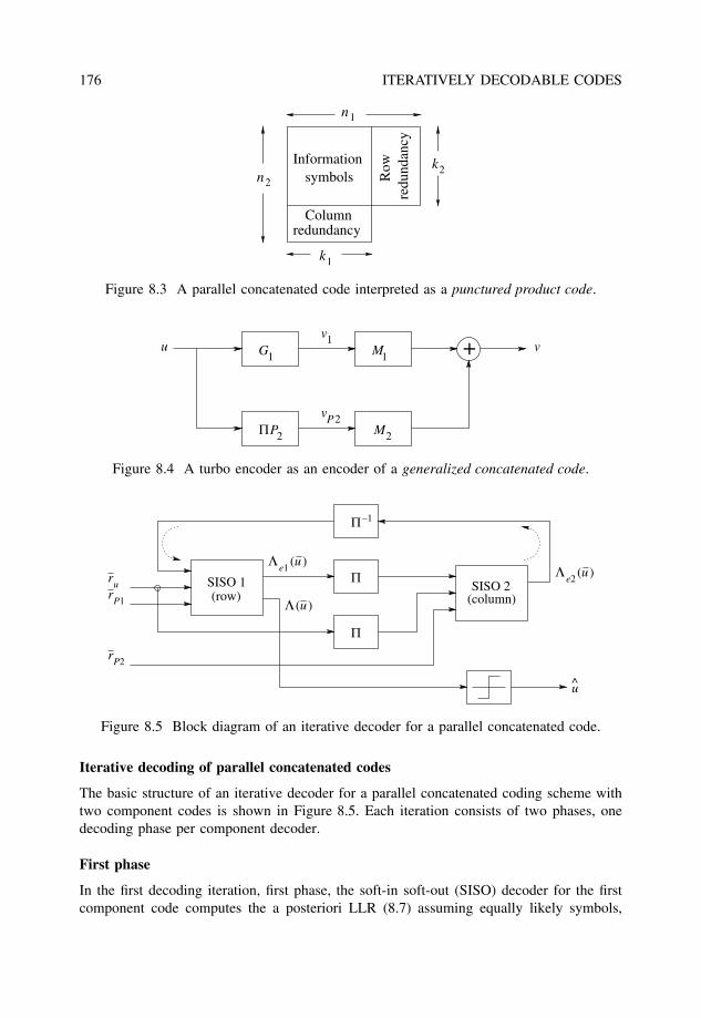
176 ITERATIVELY DECODABLE CODES
Informationsymbols
Columnredundancy
Row
redu
ndan
cy
k1
n1
n2
k2
Figure 8.3 A parallel concatenated code interpreted as a punctured product code.
2
G1
PΠ
+u 1v
vP2
M1
M2
v
Figure 8.4 A turbo encoder as an encoder of a generalized concatenated code.
Λe1 (u )
Λe2 (u )Π
Π
rr
Π−1
Λ(u )
r
u
P1
P2
u
(column)SISO 2 SISO 1
(row)
Figure 8.5 Block diagram of an iterative decoder for a parallel concatenated code.
Iterative decoding of parallel concatenated codes
The basic structure of an iterative decoder for a parallel concatenated coding scheme withtwo component codes is shown in Figure 8.5. Each iteration consists of two phases, onedecoding phase per component decoder.
First phase
In the first decoding iteration, first phase, the soft-in soft-out (SISO) decoder for the firstcomponent code computes the a posteriori LLR (8.7) assuming equally likely symbols,
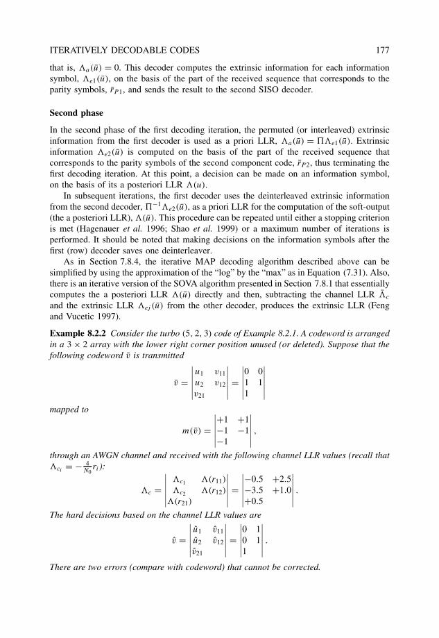
ITERATIVELY DECODABLE CODES 177
that is, �a(u) = 0. This decoder computes the extrinsic information for each informationsymbol, �e1(u), on the basis of the part of the received sequence that corresponds to theparity symbols, rP 1, and sends the result to the second SISO decoder.
Second phase
In the second phase of the first decoding iteration, the permuted (or interleaved) extrinsicinformation from the first decoder is used as a priori LLR, �a(u) = �e1(u). Extrinsicinformation �e2(u) is computed on the basis of the part of the received sequence thatcorresponds to the parity symbols of the second component code, rP 2, thus terminating thefirst decoding iteration. At this point, a decision can be made on an information symbol,on the basis of its a posteriori LLR �(u).
In subsequent iterations, the first decoder uses the deinterleaved extrinsic informationfrom the second decoder, −1�e2(u), as a priori LLR for the computation of the soft-output(the a posteriori LLR), �(u). This procedure can be repeated until either a stopping criterionis met (Hagenauer et al. 1996; Shao et al. 1999) or a maximum number of iterations isperformed. It should be noted that making decisions on the information symbols after thefirst (row) decoder saves one deinterleaver.
As in Section 7.8.4, the iterative MAP decoding algorithm described above can besimplified by using the approximation of the “log” by the “max” as in Equation (7.31). Also,there is an iterative version of the SOVA algorithm presented in Section 7.8.1 that essentiallycomputes the a posteriori LLR �(u) directly and then, subtracting the channel LLR �c
and the extrinsic LLR �ej (u) from the other decoder, produces the extrinsic LLR (Fengand Vucetic 1997).
Example 8.2.2 Consider the turbo (5, 2, 3) code of Example 8.2.1. A codeword is arrangedin a 3 × 2 array with the lower right corner position unused (or deleted). Suppose that thefollowing codeword v is transmitted
v =∣∣∣∣∣∣u1 v11
u2 v12
v21
∣∣∣∣∣∣ =∣∣∣∣∣∣0 01 11
∣∣∣∣∣∣mapped to
m(v) =∣∣∣∣∣∣+1 +1−1 −1−1
∣∣∣∣∣∣ ,through an AWGN channel and received with the following channel LLR values (recall that�ci
= − 4N0
ri):
�c =∣∣∣∣∣∣
�c1 �(r11)
�c2 �(r12)
�(r21)
∣∣∣∣∣∣ =∣∣∣∣∣∣−0.5 +2.5−3.5 +1.0+0.5
∣∣∣∣∣∣ .The hard decisions based on the channel LLR values are
v =∣∣∣∣∣∣u1 v11
u2 v12
v21
∣∣∣∣∣∣ =∣∣∣∣∣∣0 10 11
∣∣∣∣∣∣ .There are two errors (compare with codeword) that cannot be corrected.
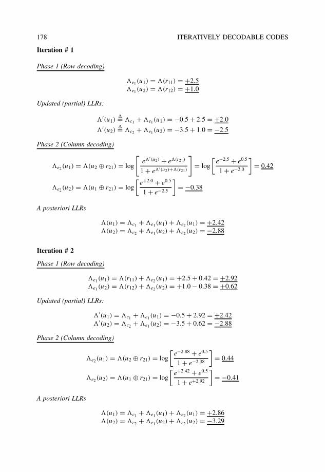
178 ITERATIVELY DECODABLE CODES
Iteration # 1
Phase 1 (Row decoding)
�e1(u1) = �(r11) = +2.5�e1(u2) = �(r12) = +1.0
Updated (partial) LLRs:
�′(u1)�= �c1 + �e1(u1) = −0.5 + 2.5 = +2.0
�′(u2)�= �c2 + �e1(u2) = −3.5 + 1.0 = −2.5
Phase 2 (Column decoding)
�e2(u1) = �(u2 ⊕ r21) = log
[e�′(u2) + e�(r21)
1 + e�′(u2)+�(r21)
]= log
[e−2.5 + e0.5
1 + e−2.0
]= 0.42
�e2(u2) = �(u1 ⊕ r21) = log
[e+2.0 + e0.5
1 + e−2.5
]= −0.38
A posteriori LLRs
�(u1) = �c1 + �e1(u1) + �e2(u1) = +2.42�(u2) = �c2 + �e1(u2) + �e2(u2) = −2.88
Iteration # 2
Phase 1 (Row decoding)
�e1(u1) = �(r11) + �e2(u1) = +2.5 + 0.42 = +2.92�e1(u2) = �(r12) + �e2(u2) = +1.0 − 0.38 = +0.62
Updated (partial) LLRs:
�′(u1) = �c1 + �e1(u1) = −0.5 + 2.92 = +2.42�′(u2) = �c2 + �e1(u2) = −3.5 + 0.62 = −2.88
Phase 2 (Column decoding)
�e2(u1) = �(u2 ⊕ r21) = log
[e−2.88 + e0.5
1 + e−2.38
]= 0.44
�e2(u2) = �(u1 ⊕ r21) = log
[e+2.42 + e0.5
1 + e+2.92
]= −0.41
A posteriori LLRs
�(u1) = �c1 + �e1(u1) + �e2(u1) = +2.86�(u2) = �c2 + �e1(u2) + �e2(u2) = −3.29
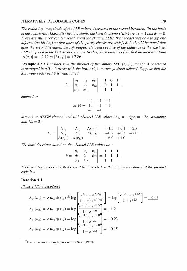
ITERATIVELY DECODABLE CODES 179
The reliability (magnitude of the LLR values) increases in the second iteration. On the basisof the a posteriori LLRs after two iterations, the hard decisions (HDs) are u1 = 1 and u2 = 0.These are still incorrect. However, given the channel LLRs, the decoder was able to flip oneinformation bit (u1) so that most of the parity checks are satisfied. It should be noted thatafter the second iteration, the soft outputs changed because of the influence of the extrinsicLLR computed in the first iteration. In particular, the reliability of the first bit increases from|�(u1)| = +2.42 to |�(u1)| = +2.86.
Example 8.2.3 Consider now the product of two binary SPC (3,2,2) codes.7 A codewordis arranged in a 3 × 3 array with the lower right corner position deleted. Suppose that thefollowing codeword v is transmitted
v =∣∣∣∣∣∣u1 u2 v11
u3 u4 v12
v21 v22
∣∣∣∣∣∣ =∣∣∣∣∣∣1 0 10 1 11 1
∣∣∣∣∣∣ ,mapped to
m(v) =∣∣∣∣∣∣−1 +1 −1+1 −1 −1−1 −1
∣∣∣∣∣∣ ,through an AWGN channel and with channel LLR values (�ci
= − 4N0
ri = −2ri , assumingthat N0 = 2):
�c =∣∣∣∣∣∣
�c1 �c2 �(r11)
�c3 �c4 �(r12)
�(r21) �(r22)
∣∣∣∣∣∣ =∣∣∣∣∣∣+1.5 +0.1 +2.5+0.2 +0.3 +2.0+6.0 +1.0
∣∣∣∣∣∣ .The hard decisions based on the channel LLR values are:
v =∣∣∣∣∣∣u1 u2 v11
u3 u4 v12
v21 v22
∣∣∣∣∣∣ =∣∣∣∣∣∣1 1 11 1 11 1
∣∣∣∣∣∣ .There are two errors in v that cannot be corrected as the minimum distance of the productcode is 4.
Iteration # 1
Phase 1 (Row decoding)
�e1(u1) = �(u2 ⊕ r11)�= log
[e�c2 + e�(r11)
1 + e�c2 +�(r21)
]= log
[e+0.1 + e+2.5
1 + e+2.6
]= −0.08
�e1(u2) = �(u1 ⊕ r11) = log
[e+1.5 + e+2.5
1 + e+4.0
]= −1.2
�e1(u3) = �(u4 ⊕ r12) = log
[e+0.3 + e+2.0
1 + e+2.3
]= −0.23
�e1(u4) = �(u3 ⊕ r12) = log
[e+0.2 + e+2.0
1 + e+2.2
]= −0.15
7This is the same example presented in Sklar (1997).
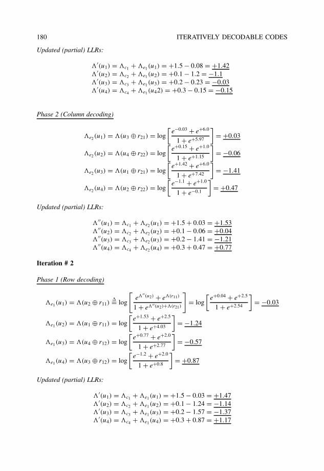
180 ITERATIVELY DECODABLE CODES
Updated (partial) LLRs:
�′(u1) = �c1 + �e1(u1) = +1.5 − 0.08 = +1.42�′(u2) = �c2 + �e1(u2) = +0.1 − 1.2 = −1.1�′(u3) = �c3 + �e1(u3) = +0.2 − 0.23 = −0.03�′(u4) = �c4 + �e1(u42) = +0.3 − 0.15 = −0.15
Phase 2 (Column decoding)
�e2(u1) = �(u3 ⊕ r21) = log
[e−0.03 + e+6.0
1 + e+5.97
]= +0.03
�e2(u2) = �(u4 ⊕ r22) = log
[e+0.15 + e+1.0
1 + e+1.15
]= −0.06
�e2(u3) = �(u1 ⊕ r21) = log
[e+1.42 + e+6.0
1 + e+7.42
]= −1.41
�e2(u4) = �(u2 ⊕ r22) = log
[e−1.1 + e+1.0
1 + e−0.1
]= +0.47
Updated (partial) LLRs:
�′′(u1) = �c1 + �e2(u1) = +1.5 + 0.03 = +1.53�′′(u2) = �c2 + �e2(u2) = +0.1 − 0.06 = +0.04�′′(u3) = �c3 + �e2(u3) = +0.2 − 1.41 = −1.21�′′(u4) = �c4 + �e2(u4) = +0.3 + 0.47 = +0.77
Iteration # 2
Phase 1 (Row decoding)
�e1(u1) = �(u2 ⊕ r11)�= log
[e�′′(u2) + e�(r11)
1 + e�′′(u2)+�(r21)
]= log
[e+0.04 + e+2.5
1 + e+2.54
]= −0.03
�e1(u2) = �(u1 ⊕ r11) = log
[e+1.53 + e+2.5
1 + e+4.03
]= −1.24
�e1(u3) = �(u4 ⊕ r12) = log
[e+0.77 + e+2.0
1 + e+2.77
]= −0.57
�e1(u4) = �(u3 ⊕ r12) = log
[e−1.2 + e+2.0
1 + e+0.8
]= +0.87
Updated (partial) LLRs:
�′(u1) = �c1 + �e1(u1) = +1.5 − 0.03 = +1.47�′(u2) = �c2 + �e1(u2) = +0.1 − 1.24 = −1.14�′(u3) = �c3 + �e1(u3) = +0.2 − 1.57 = −1.37�′(u4) = �c4 + �e1(u4) = +0.3 + 0.87 = +1.17
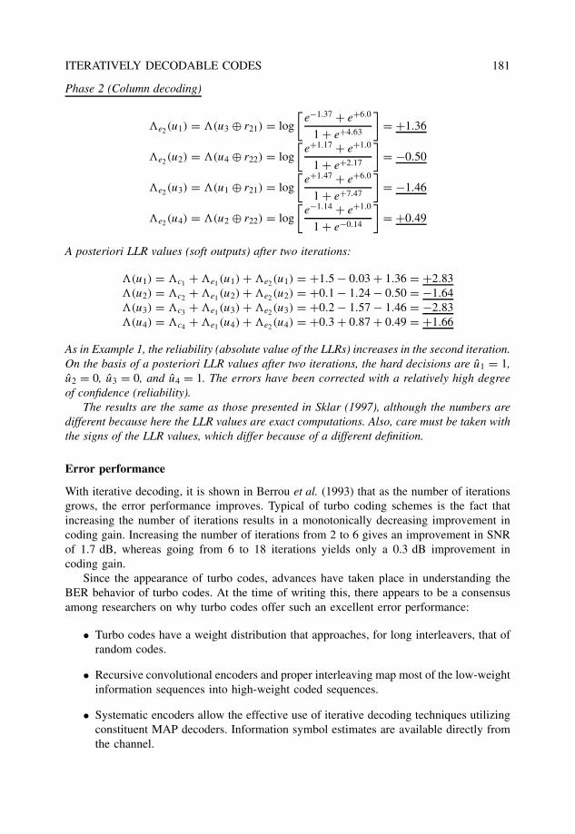
ITERATIVELY DECODABLE CODES 181
Phase 2 (Column decoding)
�e2(u1) = �(u3 ⊕ r21) = log
[e−1.37 + e+6.0
1 + e+4.63
]= +1.36
�e2(u2) = �(u4 ⊕ r22) = log
[e+1.17 + e+1.0
1 + e+2.17
]= −0.50
�e2(u3) = �(u1 ⊕ r21) = log
[e+1.47 + e+6.0
1 + e+7.47
]= −1.46
�e2(u4) = �(u2 ⊕ r22) = log
[e−1.14 + e+1.0
1 + e−0.14
]= +0.49
A posteriori LLR values (soft outputs) after two iterations:
�(u1) = �c1 + �e1(u1) + �e2(u1) = +1.5 − 0.03 + 1.36 = +2.83�(u2) = �c2 + �e1(u2) + �e2(u2) = +0.1 − 1.24 − 0.50 = −1.64�(u3) = �c3 + �e1(u3) + �e2(u3) = +0.2 − 1.57 − 1.46 = −2.83�(u4) = �c4 + �e1(u4) + �e2(u4) = +0.3 + 0.87 + 0.49 = +1.66
As in Example 1, the reliability (absolute value of the LLRs) increases in the second iteration.On the basis of a posteriori LLR values after two iterations, the hard decisions are u1 = 1,u2 = 0, u3 = 0, and u4 = 1. The errors have been corrected with a relatively high degreeof confidence (reliability).
The results are the same as those presented in Sklar (1997), although the numbers aredifferent because here the LLR values are exact computations. Also, care must be taken withthe signs of the LLR values, which differ because of a different definition.
Error performance
With iterative decoding, it is shown in Berrou et al. (1993) that as the number of iterationsgrows, the error performance improves. Typical of turbo coding schemes is the fact thatincreasing the number of iterations results in a monotonically decreasing improvement incoding gain. Increasing the number of iterations from 2 to 6 gives an improvement in SNRof 1.7 dB, whereas going from 6 to 18 iterations yields only a 0.3 dB improvement incoding gain.
Since the appearance of turbo codes, advances have taken place in understanding theBER behavior of turbo codes. At the time of writing this, there appears to be a consensusamong researchers on why turbo codes offer such an excellent error performance:
• Turbo codes have a weight distribution that approaches, for long interleavers, that ofrandom codes.
• Recursive convolutional encoders and proper interleaving map most of the low-weightinformation sequences into high-weight coded sequences.
• Systematic encoders allow the effective use of iterative decoding techniques utilizingconstituent MAP decoders. Information symbol estimates are available directly fromthe channel.
182 ITERATIVELY DECODABLE CODES
In addition, a number of interesting semianalytical tools have appeared, in density evo-lution (Richardson and Urbanke 2001), Gaussian approximation (Gamal and Hammons2001), and mutual information (ten Brink 1999, 2001) or SNR transfer (Divsalar et al.2001) characteristics, to study the convergence properties of iterative decoding algorithms.
The art of interleaving
A critical component in achieving good performance with iterative decoding of a turbo codeis the interleaver. In turbo codes, the interleaver serves three main purposes: (1) build verylong codes with weight distributions that approach those of random codes, (2) help in theiterative decoding process by decorrelating the input LLRs to the SISO decoders as muchas possible, and (3) proper termination of the trellis in a known state, after the transmissionof short to medium length frames, to avoid edge effects that increase the multiplicity oflow-weight paths in the trellises of the component codes. To emphasize, the specific typeof interleaver becomes an important factor to consider as the frame lengths (or interleaverlengths) become relatively small, say, up to one thousand symbols. There is a wealth ofpublications devoted to interleaver design for turbo codes. In this section, a brief descriptionof the basic interleaver types and pointers to the literature are given.
In 1970, several types of optimum interleavers were introduced (Ramsey 1970). Inparticular, an (n1, n2) interleaver was defined as a device that “reorders a sequence so thatno contiguous sequence of n2 symbols in the reordered sequence contains any symbols thatare separated by fewer than n1 symbols in the original ordering.”
Let . . . , a�1 , a�2, a�3, . . . denote the output sequence from an (n1, n2) interleaver, where�1, �2, . . . are the positions of these symbols in the input sequence. Then the definition inthe previous paragraph translates into the following condition:
|�i − �j | ≥ n1
whenever|i − j | < n2.
It can be shown that the deinterleaver of an (n1, n2) interleaver is itself an (n1, n2) inter-leaver. The delay of the interleaver and deinterleaver are both equal to the delay introducedby the overall interleaving–deinterleaving operation. Another important parameter of aninterleaver is the amount of storage or memory required. Ramsey showed four types of(n1, n2) interleavers that are optimum in the sense of minimizing the delay and memoryrequired to implement them. These interleavers are known as Ramsey interleavers. At aboutthe same time, Forney (1971) proposed an interleaver with the same basic structure of an(n1, n2) Ramsey interleaver, known as a convolutional interleaver. Convolutional inter-leavers were discussed in Section 6.2.4 and have been applied to the design of good turbocoding schemes (Hall and Wilson 2001).
There are several novel approaches to the analysis and design of interleavers: oneis based on a random interleaver with a spreading property. Such a structure was firstproposed in Divsalar and Pollara (1993), together with a simple algorithm to constructS-random interleavers: Generate random integers in the range [1, N ], and use a constrainton the interleaving distance. This constraint is seen to be equivalent to the definition of aRamsey (S2, S1 + 1) interleaver (this is noted in Vucetic and J. Yuan (2000), pp. 211–213).Additional constraints, for example, based on the empirical correlation between successive
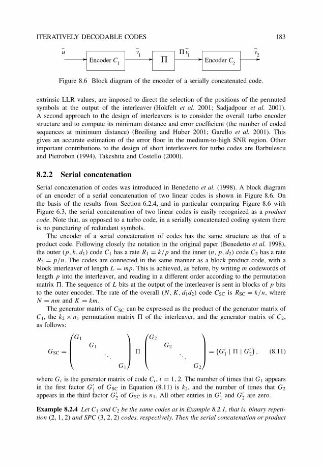
ITERATIVELY DECODABLE CODES 183
Πv1 v2
Encoder C Encoder C21
Π v1u
Figure 8.6 Block diagram of the encoder of a serially concatenated code.
extrinsic LLR values, are imposed to direct the selection of the positions of the permutedsymbols at the output of the interleaver (Hokfelt et al. 2001; Sadjadpour et al. 2001).A second approach to the design of interleavers is to consider the overall turbo encoderstructure and to compute its minimum distance and error coefficient (the number of codedsequences at minimum distance) (Breiling and Huber 2001; Garello et al. 2001). Thisgives an accurate estimation of the error floor in the medium-to-high SNR region. Otherimportant contributions to the design of short interleavers for turbo codes are Barbulescuand Pietrobon (1994), Takeshita and Costello (2000).
8.2.2 Serial concatenation
Serial concatenation of codes was introduced in Benedetto et al. (1998). A block diagramof an encoder of a serial concatenation of two linear codes is shown in Figure 8.6. Onthe basis of the results from Section 6.2.4, and in particular comparing Figure 8.6 withFigure 6.3, the serial concatenation of two linear codes is easily recognized as a productcode. Note that, as opposed to a turbo code, in a serially concatenated coding system thereis no puncturing of redundant symbols.
The encoder of a serial concatenation of codes has the same structure as that of aproduct code. Following closely the notation in the original paper (Benedetto et al. 1998),the outer (p, k, d1) code C1 has a rate R1 = k/p and the inner (n, p, d2) code C2 has a rateR2 = p/n. The codes are connected in the same manner as a block product code, with ablock interleaver of length L = mp. This is achieved, as before, by writing m codewords oflength p into the interleaver, and reading in a different order according to the permutationmatrix . The sequence of L bits at the output of the interleaver is sent in blocks of p bitsto the outer encoder. The rate of the overall (N, K, d1d2) code CSC is RSC = k/n, whereN = nm and K = km.
The generator matrix of CSC can be expressed as the product of the generator matrix ofC1, the k2 × n1 permutation matrix of the interleaver, and the generator matrix of C2,as follows:
GSC =
G1
G1
. . .
G1
G2
G2
. . .
G2
= (
G′1 | | G′
2
), (8.11)
where Gi is the generator matrix of code Ci , i = 1, 2. The number of times that G1 appearsin the first factor G′
1 of GSC in Equation (8.11) is k2, and the number of times that G2
appears in the third factor G′2 of GSC is n1. All other entries in G′
1 and G′2 are zero.
Example 8.2.4 Let C1 and C2 be the same codes as in Example 8.2.1, that is, binary repeti-tion (2, 1, 2) and SPC (3, 2, 2) codes, respectively. Then the serial concatenation or product
184 ITERATIVELY DECODABLE CODES
of C1 and C2, CSC, is a binary linear block (6, 2, 4) code. Note that the minimum distance ofCSC is larger than that of CPC in Example 8.2.1. The generator matrices are G1 = (
1 1)
and G2 =(
1 0 10 1 1
). Assuming that a conventional product code is employed, the per-
mutation matrix, associated with a row-by-row and column-by-column interleaver, is
=
1 0 0 00 0 1 00 1 0 00 0 0 1
.
Therefore, the generator matrix of CSC is
GSC =((
1 1)
012
012(1 1
))
1 0 0 00 0 1 00 1 0 00 0 0 1
(1 0 10 1 1
)023
023
(1 0 10 1 1
)
=(
1 0 1 00 1 0 1
)
(1 0 10 1 1
)023
023
(1 0 10 1 1
)
=((
1 0 1) (
1 0 1)(
0 1 1) (
0 1 1))
=((
1 0 10 1 1
) (1 0 10 1 1
)),
where 0ij denotes the i × j all-zero matrix.The result can be verified by noticing that the last equality contains the generator matrix
of the SPC (3, 2, 2) code twice because of the repetition (2, 1, 2) code. It is also interesting tonote that this is the smallest member of the family of repeat-and-accumulate codes (Divsalaret al. 1998).
It should be noted that the main difference between the serial concatenated codingscheme and product coding discussed in Section 6.2.4 is that the interleaver was either arow-by-row column-by-column interleaver or a cyclic interleaver (if the component codeswere cyclic). In contrast, as with turbo codes, the good performance of serial concatenationschemes generally depends on an interleaver that is chosen as “randomly” as possible.
Contrary to turbo codes, serially concatenated codes do not exhibit “interleaver gainsaturation” (i.e., there is no error floor). Using a random argument for interleavers oflength N , it can be shown that the error probability for a product code contains a factorN−[(dOf +1)/2], where dOf denotes the minimum distance of the outer code as opposed to afactor N−1 for parallel concatenated codes (Benedetto et al. 1998).
As a result, product codes outperform turbo codes in the SNR region where the errorfloor appears. At low SNR values, however, the better weight distribution properties ofturbo codes (Perez et al. 1996) leads to better performance than product codes.
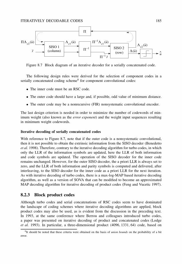
ITERATIVELY DECODABLE CODES 185
rΠ−1
Λe1 (u)
Λe2 (u)
u
Π
Π Λ(u)
−1ΠΠΛe2 (u) Λ
e1 (u)
r (column)SISO 1
(row)SISO 2 −1
Figure 8.7 Block diagram of an iterative decoder for a serially concatenated code.
The following design rules were derived for the selection of component codes in aserially concatenated coding scheme8 for component convolutional codes:
• The inner code must be an RSC code.
• The outer code should have a large and, if possible, odd value of minimum distance.
• The outer code may be a nonrecursive (FIR) nonsystematic convolutional encoder.
The last design criterion is needed in order to minimize the number of codewords of min-imum weight (also known as the error exponent) and the weight input sequences resultingin minimum weight codewords.
Iterative decoding of serially concatenated codes
With reference to Figure 8.7, note that if the outer code is a nonsystematic convolutional,then it is not possible to obtain the extrinsic information from the SISO decoder (Benedettoet al. 1998). Therefore, contrary to the iterative decoding algorithm for turbo codes, in whichonly the LLR of the information symbols are updated, here the LLR of both informationand code symbols are updated. The operation of the SISO decoder for the inner coderemains unchanged. However, for the outer SISO decoder, the a priori LLR is always set tozero, and the LLR of both information and parity symbols is computed and delivered, afterinterleaving, to the SISO decoder for the inner code as a priori LLR for the next iteration.As with iterative decoding of turbo codes, there is a max-log-MAP based iterative decodingalgorithm, as well as a version of SOVA that can be modified to become an approximatedMAP decoding algorithm for iterative decoding of product codes (Feng and Vucetic 1997).
8.2.3 Block product codes
Although turbo codes and serial concatenations of RSC codes seem to have dominatedthe landscape of coding schemes where iterative decoding algorithms are applied, blockproduct codes may also be used, as is evident from the discussion in the preceding text.In 1993, at the same conference where Berrou and colleagues introduced turbo codes,a paper was presented on iterative decoding of product and concatenated codes (Lodgeet al. 1993). In particular, a three-dimensional product (4096, 1331, 64) code, based on
8It should be noted that these criteria were obtained on the basis of union bounds on the probability of a biterror.
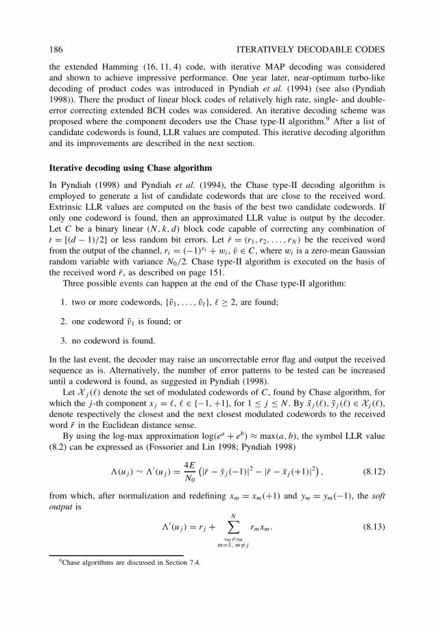
186 ITERATIVELY DECODABLE CODES
the extended Hamming (16, 11, 4) code, with iterative MAP decoding was consideredand shown to achieve impressive performance. One year later, near-optimum turbo-likedecoding of product codes was introduced in Pyndiah et al. (1994) (see also (Pyndiah1998)). There the product of linear block codes of relatively high rate, single- and double-error correcting extended BCH codes was considered. An iterative decoding scheme wasproposed where the component decoders use the Chase type-II algorithm.9 After a list ofcandidate codewords is found, LLR values are computed. This iterative decoding algorithmand its improvements are described in the next section.
Iterative decoding using Chase algorithm
In Pyndiah (1998) and Pyndiah et al. (1994), the Chase type-II decoding algorithm isemployed to generate a list of candidate codewords that are close to the received word.Extrinsic LLR values are computed on the basis of the best two candidate codewords. Ifonly one codeword is found, then an approximated LLR value is output by the decoder.Let C be a binary linear (N, k, d) block code capable of correcting any combination oft = [(d − 1)/2] or less random bit errors. Let r = (r1, r2, . . . , rN) be the received wordfrom the output of the channel, ri = (−1)vi + wi , v ∈ C, where wi is a zero-mean Gaussianrandom variable with variance N0/2. Chase type-II algorithm is executed on the basis ofthe received word r , as described on page 151.
Three possible events can happen at the end of the Chase type-II algorithm:
1. two or more codewords, {v1, . . . , v�}, � ≥ 2, are found;
2. one codeword v1 is found; or
3. no codeword is found.
In the last event, the decoder may raise an uncorrectable error flag and output the receivedsequence as is. Alternatively, the number of error patterns to be tested can be increaseduntil a codeword is found, as suggested in Pyndiah (1998).
Let X j (�) denote the set of modulated codewords of C, found by Chase algorithm, forwhich the j -th component xj = �, � ∈ {−1, +1}, for 1 ≤ j ≤ N . By xj (�), yj (�) ∈ Xj (�),denote respectively the closest and the next closest modulated codewords to the receivedword r in the Euclidean distance sense.
By using the log-max approximation log(ea + eb) ≈ max(a, b), the symbol LLR value(8.2) can be expressed as (Fossorier and Lin 1998; Pyndiah 1998)
�(uj ) ∼ �′(uj ) = 4E
N0
(|r − yj (−1)|2 − |r − xj (+1)|2) , (8.12)
from which, after normalization and redefining xm = xm(+1) and ym = ym(−1), the softoutput is
�′(uj ) = rj +N∑
xm �=ymm=1, m�=j
rmxm. (8.13)
9Chase algorithms are discussed in Section 7.4.
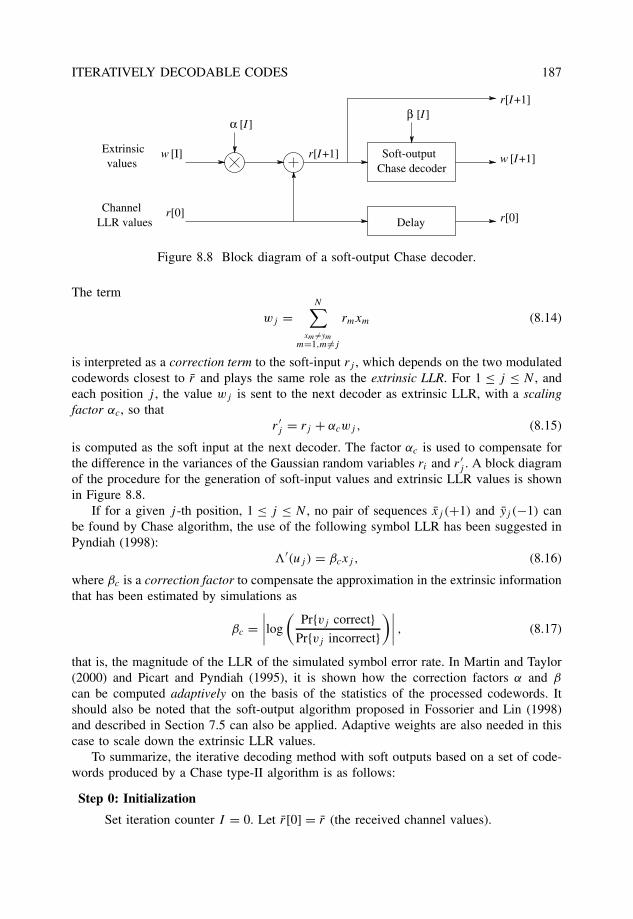
ITERATIVELY DECODABLE CODES 187
r
[I+1]w
[0]
w
α [I ]
r[I+1]
r[0]ChannelLLR values
Extrinsicvalues
[I]
β [I ]
Soft-outputChase decoder
Delay
[I+1]r
Figure 8.8 Block diagram of a soft-output Chase decoder.
The term
wj =N∑
xm �=ymm=1,m�=j
rmxm (8.14)
is interpreted as a correction term to the soft-input rj , which depends on the two modulatedcodewords closest to r and plays the same role as the extrinsic LLR. For 1 ≤ j ≤ N , andeach position j , the value wj is sent to the next decoder as extrinsic LLR, with a scalingfactor αc, so that
r ′j = rj + αcwj , (8.15)
is computed as the soft input at the next decoder. The factor αc is used to compensate forthe difference in the variances of the Gaussian random variables ri and r ′
j . A block diagramof the procedure for the generation of soft-input values and extrinsic LLR values is shownin Figure 8.8.
If for a given j -th position, 1 ≤ j ≤ N , no pair of sequences xj (+1) and yj (−1) canbe found by Chase algorithm, the use of the following symbol LLR has been suggested inPyndiah (1998):
�′(uj ) = βcxj , (8.16)
where βc is a correction factor to compensate the approximation in the extrinsic informationthat has been estimated by simulations as
βc =∣∣∣∣log
(Pr{vj correct}
Pr{vj incorrect})∣∣∣∣ , (8.17)
that is, the magnitude of the LLR of the simulated symbol error rate. In Martin and Taylor(2000) and Picart and Pyndiah (1995), it is shown how the correction factors α and β
can be computed adaptively on the basis of the statistics of the processed codewords. Itshould also be noted that the soft-output algorithm proposed in Fossorier and Lin (1998)and described in Section 7.5 can also be applied. Adaptive weights are also needed in thiscase to scale down the extrinsic LLR values.
To summarize, the iterative decoding method with soft outputs based on a set of code-words produced by a Chase type-II algorithm is as follows:
Step 0: Initialization
Set iteration counter I = 0. Let r[0] = r (the received channel values).
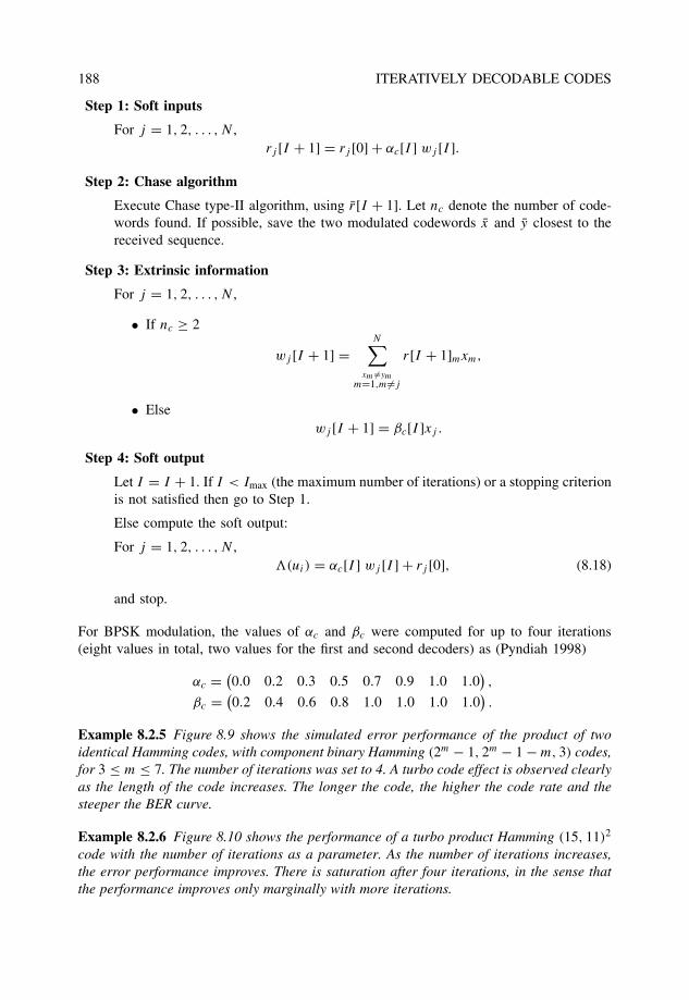
188 ITERATIVELY DECODABLE CODES
Step 1: Soft inputs
For j = 1, 2, . . . , N ,rj [I + 1] = rj [0] + αc[I ] wj [I ].
Step 2: Chase algorithm
Execute Chase type-II algorithm, using r[I + 1]. Let nc denote the number of code-words found. If possible, save the two modulated codewords x and y closest to thereceived sequence.
Step 3: Extrinsic information
For j = 1, 2, . . . , N ,
• If nc ≥ 2
wj [I + 1] =N∑
xm �=ymm=1,m�=j
r[I + 1]mxm,
• Elsewj [I + 1] = βc[I ]xj .
Step 4: Soft output
Let I = I + 1. If I < Imax (the maximum number of iterations) or a stopping criterionis not satisfied then go to Step 1.
Else compute the soft output:
For j = 1, 2, . . . , N ,�(ui) = αc[I ] wj [I ] + rj [0], (8.18)
and stop.
For BPSK modulation, the values of αc and βc were computed for up to four iterations(eight values in total, two values for the first and second decoders) as (Pyndiah 1998)
αc = (0.0 0.2 0.3 0.5 0.7 0.9 1.0 1.0
),
βc = (0.2 0.4 0.6 0.8 1.0 1.0 1.0 1.0
).
Example 8.2.5 Figure 8.9 shows the simulated error performance of the product of twoidentical Hamming codes, with component binary Hamming (2m − 1, 2m − 1 − m, 3) codes,for 3 ≤ m ≤ 7. The number of iterations was set to 4. A turbo code effect is observed clearlyas the length of the code increases. The longer the code, the higher the code rate and thesteeper the BER curve.
Example 8.2.6 Figure 8.10 shows the performance of a turbo product Hamming (15, 11)2
code with the number of iterations as a parameter. As the number of iterations increases,the error performance improves. There is saturation after four iterations, in the sense thatthe performance improves only marginally with more iterations.
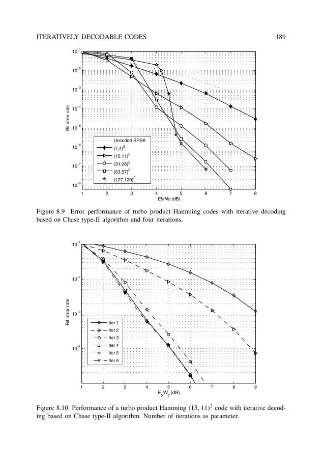
ITERATIVELY DECODABLE CODES 189
1 2 3 4 5 6 7 8
10−8
10−7
10−6
10−5
10−4
10−3
10−2
10−1
Eb/No (dB)
Bit
erro
r ra
te
Uncoded BPSK
(7,4)2
(15,11)2
(31,26)2
(63,57)2
(127,120)2
Figure 8.9 Error performance of turbo product Hamming codes with iterative decodingbased on Chase type-II algorithm and four iterations.
1 2 3 4 5 6 7 8 9
10−4
10−3
10−2
10−1
Eb/N
0 (dB)
Bit
erro
r ra
te
Iter 1
Iter 2
Iter 3
Iter 4
Iter 5
Iter 6
Figure 8.10 Performance of a turbo product Hamming (15, 11)2 code with iterative decod-ing based on Chase type-II algorithm. Number of iterations as parameter.
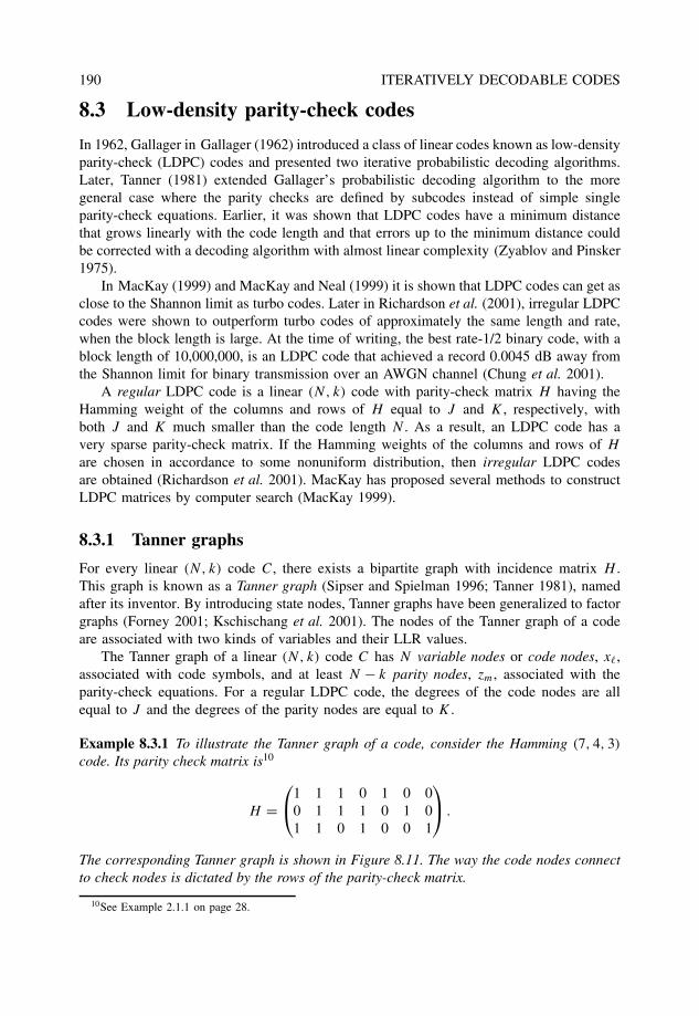
190 ITERATIVELY DECODABLE CODES
8.3 Low-density parity-check codes
In 1962, Gallager in Gallager (1962) introduced a class of linear codes known as low-densityparity-check (LDPC) codes and presented two iterative probabilistic decoding algorithms.Later, Tanner (1981) extended Gallager’s probabilistic decoding algorithm to the moregeneral case where the parity checks are defined by subcodes instead of simple singleparity-check equations. Earlier, it was shown that LDPC codes have a minimum distancethat grows linearly with the code length and that errors up to the minimum distance couldbe corrected with a decoding algorithm with almost linear complexity (Zyablov and Pinsker1975).
In MacKay (1999) and MacKay and Neal (1999) it is shown that LDPC codes can get asclose to the Shannon limit as turbo codes. Later in Richardson et al. (2001), irregular LDPCcodes were shown to outperform turbo codes of approximately the same length and rate,when the block length is large. At the time of writing, the best rate-1/2 binary code, with ablock length of 10,000,000, is an LDPC code that achieved a record 0.0045 dB away fromthe Shannon limit for binary transmission over an AWGN channel (Chung et al. 2001).
A regular LDPC code is a linear (N, k) code with parity-check matrix H having theHamming weight of the columns and rows of H equal to J and K , respectively, withboth J and K much smaller than the code length N . As a result, an LDPC code has avery sparse parity-check matrix. If the Hamming weights of the columns and rows of H
are chosen in accordance to some nonuniform distribution, then irregular LDPC codesare obtained (Richardson et al. 2001). MacKay has proposed several methods to constructLDPC matrices by computer search (MacKay 1999).
8.3.1 Tanner graphs
For every linear (N, k) code C, there exists a bipartite graph with incidence matrix H .This graph is known as a Tanner graph (Sipser and Spielman 1996; Tanner 1981), namedafter its inventor. By introducing state nodes, Tanner graphs have been generalized to factorgraphs (Forney 2001; Kschischang et al. 2001). The nodes of the Tanner graph of a codeare associated with two kinds of variables and their LLR values.
The Tanner graph of a linear (N, k) code C has N variable nodes or code nodes, x�,associated with code symbols, and at least N − k parity nodes, zm, associated with theparity-check equations. For a regular LDPC code, the degrees of the code nodes are allequal to J and the degrees of the parity nodes are equal to K .
Example 8.3.1 To illustrate the Tanner graph of a code, consider the Hamming (7, 4, 3)
code. Its parity check matrix is10
H =1 1 1 0 1 0 0
0 1 1 1 0 1 01 1 0 1 0 0 1
.
The corresponding Tanner graph is shown in Figure 8.11. The way the code nodes connectto check nodes is dictated by the rows of the parity-check matrix.
10See Example 2.1.1 on page 28.
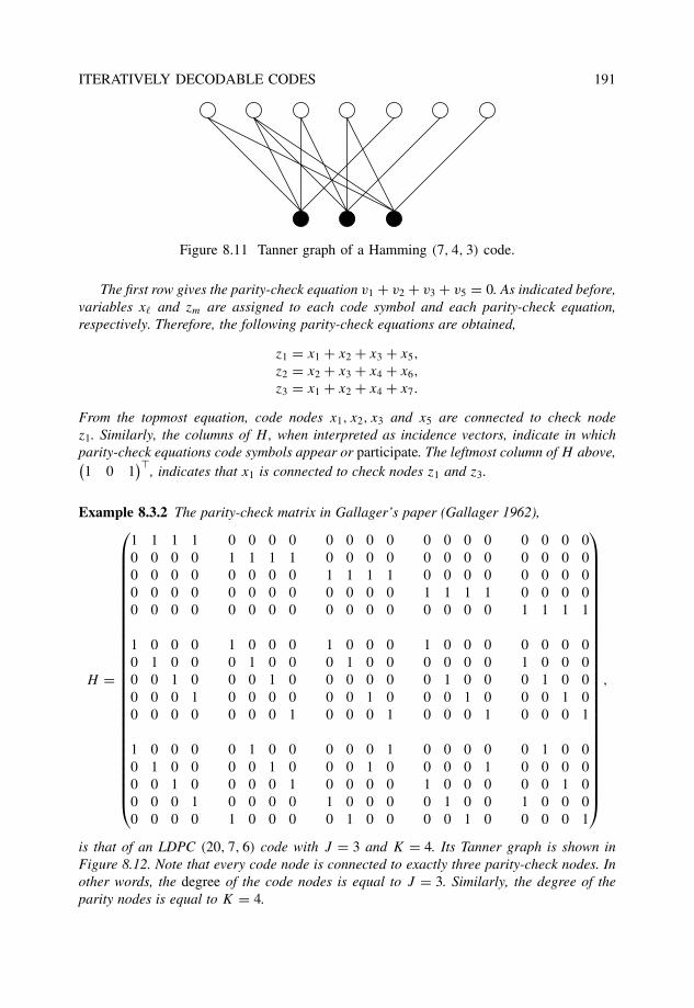
ITERATIVELY DECODABLE CODES 191
Figure 8.11 Tanner graph of a Hamming (7, 4, 3) code.
The first row gives the parity-check equation v1 + v2 + v3 + v5 = 0. As indicated before,variables x� and zm are assigned to each code symbol and each parity-check equation,respectively. Therefore, the following parity-check equations are obtained,
z1 = x1 + x2 + x3 + x5,
z2 = x2 + x3 + x4 + x6,
z3 = x1 + x2 + x4 + x7.
From the topmost equation, code nodes x1, x2, x3 and x5 are connected to check nodez1. Similarly, the columns of H , when interpreted as incidence vectors, indicate in whichparity-check equations code symbols appear or participate. The leftmost column of H above,(1 0 1
), indicates that x1 is connected to check nodes z1 and z3.
Example 8.3.2 The parity-check matrix in Gallager’s paper (Gallager 1962),
H =
1 1 1 1 0 0 0 0 0 0 0 0 0 0 0 0 0 0 0 00 0 0 0 1 1 1 1 0 0 0 0 0 0 0 0 0 0 0 00 0 0 0 0 0 0 0 1 1 1 1 0 0 0 0 0 0 0 00 0 0 0 0 0 0 0 0 0 0 0 1 1 1 1 0 0 0 00 0 0 0 0 0 0 0 0 0 0 0 0 0 0 0 1 1 1 1
1 0 0 0 1 0 0 0 1 0 0 0 1 0 0 0 0 0 0 00 1 0 0 0 1 0 0 0 1 0 0 0 0 0 0 1 0 0 00 0 1 0 0 0 1 0 0 0 0 0 0 1 0 0 0 1 0 00 0 0 1 0 0 0 0 0 0 1 0 0 0 1 0 0 0 1 00 0 0 0 0 0 0 1 0 0 0 1 0 0 0 1 0 0 0 1
1 0 0 0 0 1 0 0 0 0 0 1 0 0 0 0 0 1 0 00 1 0 0 0 0 1 0 0 0 1 0 0 0 0 1 0 0 0 00 0 1 0 0 0 0 1 0 0 0 0 1 0 0 0 0 0 1 00 0 0 1 0 0 0 0 1 0 0 0 0 1 0 0 1 0 0 00 0 0 0 1 0 0 0 0 1 0 0 0 0 1 0 0 0 0 1
,
is that of an LDPC (20, 7, 6) code with J = 3 and K = 4. Its Tanner graph is shown inFigure 8.12. Note that every code node is connected to exactly three parity-check nodes. Inother words, the degree of the code nodes is equal to J = 3. Similarly, the degree of theparity nodes is equal to K = 4.
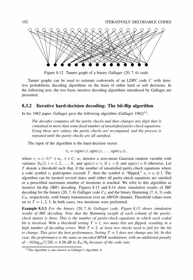
192 ITERATIVELY DECODABLE CODES
Figure 8.12 Tanner graph of a binary Gallager (20, 7, 6) code.
Tanner graphs can be used to estimate codewords of an LDPC code C with itera-tive probabilistic decoding algorithms on the basis of either hard or soft decisions. Inthe following text, the two basic iterative decoding algorithms introduced by Gallager arepresented.
8.3.2 Iterative hard-decision decoding: The bit-flip algorithm
In his 1962 paper, Gallager gave the following algorithm (Gallager 1962)11:
The decoder computes all the parity checks and then changes any digit that iscontained in more than some fixed number of unsatisfied parity-check equations.Using these new values, the parity checks are recomputed, and the process isrepeated until the parity checks are all satisfied.
The input of the algorithm is the hard-decision vector
rh = (sgn(r1), sgn(r2), . . . , sgn(rN)) ,
where ri = (−1)vi + wi , v ∈ C, wi denotes a zero-mean Gaussian random variable withvariance N0/2, i = 1, 2, . . . , N , and sgn(x) = 1, if x < 0, and sgn(x) = 0 otherwise. LetT denote a threshold such that, if the number of unsatisfied parity-check equations wherea code symbol vi participates exceeds T , then the symbol is “flipped,” vi = vi ⊕ 1. Thealgorithm can be iterated several times until either all parity-check equations are satisfiedor a prescribed maximum number of iterations is reached. We refer to this algorithm asiterative bit-flip (IBF) decoding. Figures 8.13 and 8.14 show simulation results of IBFdecoding for the binary (20, 7, 6) Gallager code CG and the binary Hamming (7, 4, 3) codeCH , respectively, with binary transmission over an AWGN channel. Threshold values wereset to T = 1, 2, 3. In both cases, two iterations were performed.
Example 8.3.3 For the binary (20, 7, 6) Gallager code, Figure 8.13 shows simulationresults of IBF decoding. Note that the Hamming weight of each column of the parity-check matrix is three. This is the number of parity-check equations in which each codedbit is involved. With a threshold setting T = 1, too many bits are flipped, resulting in ahigh number of decoding errors. With T = 2, at least two checks need to fail for the bitto change. This gives the best performance. Setting T = 3 does not change any bit. In thiscase, the performance is the same as uncoded BPSK modulation, with an additional penaltyof −10 log10(7/20) = 4.56 dB in Eb/N0 because of the code rate.
11This algorithm is also known as Gallager’s algorithm A.
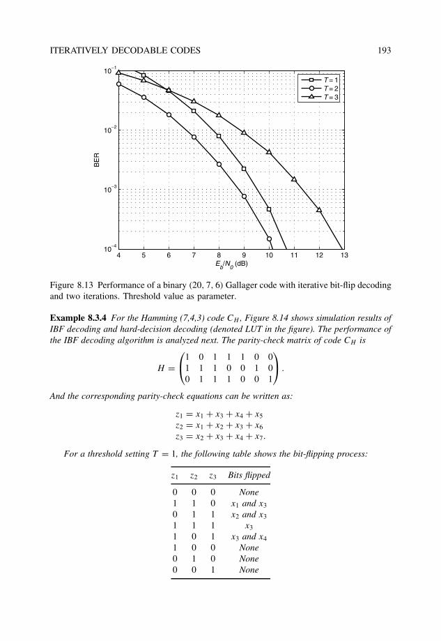
ITERATIVELY DECODABLE CODES 193
4 5 6 7 8 9 10 11 12 1310
−4
10−3
10−2
10−1
Eb/N
0 (dB)
BE
R
T = 1T = 2T = 3
Figure 8.13 Performance of a binary (20, 7, 6) Gallager code with iterative bit-flip decodingand two iterations. Threshold value as parameter.
Example 8.3.4 For the Hamming (7,4,3) code CH , Figure 8.14 shows simulation results ofIBF decoding and hard-decision decoding (denoted LUT in the figure). The performance ofthe IBF decoding algorithm is analyzed next. The parity-check matrix of code CH is
H =1 0 1 1 1 0 0
1 1 1 0 0 1 00 1 1 1 0 0 1
.
And the corresponding parity-check equations can be written as:
z1 = x1 + x3 + x4 + x5
z2 = x1 + x2 + x3 + x6
z3 = x2 + x3 + x4 + x7.
For a threshold setting T = 1, the following table shows the bit-flipping process:
z1 z2 z3 Bits flipped
0 0 0 None1 1 0 x1 and x3
0 1 1 x2 and x3
1 1 1 x3
1 0 1 x3 and x4
1 0 0 None0 1 0 None0 0 1 None
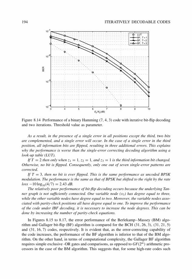
194 ITERATIVELY DECODABLE CODES
3 4 5 6 7 8 9 1010
−4
10−3
10−2
10−1
Eb/N0 (dB)
BE
R
LUTBF, T = 1BF, T = 2BF, T = 3
Figure 8.14 Performance of a binary Hamming (7, 4, 3) code with iterative bit-flip decodingand two iterations. Threshold value as parameter.
As a result, in the presence of a single error in all positions except the third, two bitsare complemented, and a single error will occur. In the case of a single error in the thirdposition, all information bits are flipped, resulting in three additional errors. This explainswhy the performance is worse than the single-error correcting decoding algorithm using alook-up table (LUT).
If T = 2 then only when z1 = 1, z2 = 1, and z3 = 1 is the third information bit changed.Otherwise, no bit is flipped. Consequently, only one out of seven single-error patterns arecorrected.
If T = 3, then no bit is ever flipped. This is the same performance as uncoded BPSKmodulation. The performance is the same as that of BPSK but shifted to the right by the rateloss −10 log10(4/7) = 2.43 dB.
The relatively poor performance of bit-flip decoding occurs because the underlying Tan-ner graph is not sufficiently connected. One variable node (x3) has degree equal to three,while the other variable nodes have degree equal to two. Moreover, the variable nodes asso-ciated with parity-check positions all have degree equal to one. To improve the performanceof the code under IBF decoding, it is necessary to increase the node degrees. This can bedone by increasing the number of parity-check equations.
In Figures 8.15 to 8.17, the error performance of the Berlekamp–Massey (BM) algo-rithm and Gallager bit-flip (BF) algorithm is compared for the BCH (31, 26, 3), (31, 21, 5)
and (31, 16, 7) codes, respectively. It is evident that, as the error-correcting capability ofthe code increases, the performance of the BF algorithm is inferior to that of the BM algo-rithm. On the other hand, in terms of computational complexity, the Gallager BF algorithmrequires simple exclusive -OR gates and comparisons, as opposed to GF(2m) arithmetic pro-cessors in the case of the BM algorithm. This suggests that, for some high-rate codes such
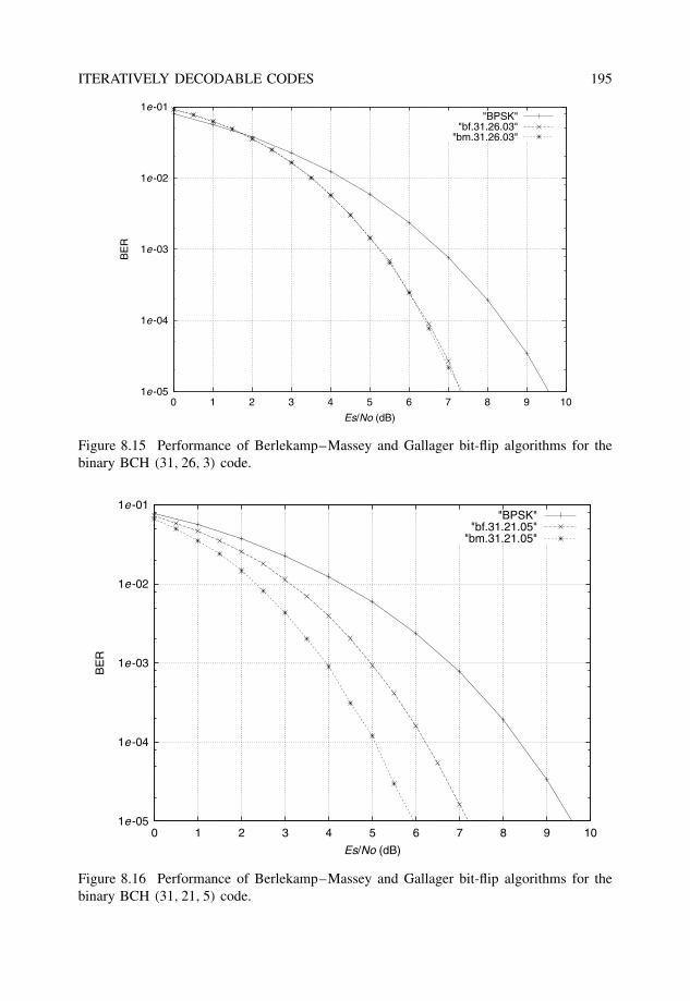
ITERATIVELY DECODABLE CODES 195
1e-05
1e-04
1e-03
1e-02
1e-01
0 1 2 3 4 5 6 7 8 9 10
BE
R
Es/No (dB)
"BPSK""bf.31.26.03"
"bm.31.26.03"
Figure 8.15 Performance of Berlekamp–Massey and Gallager bit-flip algorithms for thebinary BCH (31, 26, 3) code.
1e-05
1e-04
1e-03
1e-02
1e-01
0 1 2 3 4 5 6 7 8 9 10
BE
R
Es/No (dB)
"BPSK""bf.31.21.05"
"bm.31.21.05"
Figure 8.16 Performance of Berlekamp–Massey and Gallager bit-flip algorithms for thebinary BCH (31, 21, 5) code.
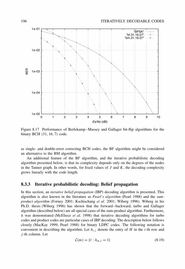
196 ITERATIVELY DECODABLE CODES
1e-05
1e-04
1e-03
1e-02
1e-01
0 1 2 3 4 5 6 7 8 9 10
BE
R
Es/No (dB)
"BPSK""bf.31.16.07"
"bm.31.16.07"
Figure 8.17 Performance of Berlekamp–Massey and Gallager bit-flip algorithms for thebinary BCH (31, 16, 7) code.
as single- and double-error correcting BCH codes, the BF algorithm might be consideredan alternative to the BM algorithm.
An additional feature of the BF algorithm, and the iterative probabilistic decodingalgorithm presented below, is that its complexity depends only on the degrees of the nodesin the Tanner graph. In other words, for fixed values of J and K , the decoding complexitygrows linearly with the code length.
8.3.3 Iterative probabilistic decoding: Belief propagation
In this section, an iterative belief-propagation (IBP) decoding algorithm is presented. Thisalgorithm is also known in the literature as Pearl’s algorithm (Pearl 1988) and the sum-product algorithm (Forney 2001; Kschischang et al. 2001; Wiberg 1996). Wiberg in hisPh.D. thesis (Wiberg 1996) has shown that the forward–backward, turbo and Gallageralgorithm (described below) are all special cases of the sum-product algorithm. Furthermore,it was demonstrated (McEliece et al. 1998) that iterative decoding algorithms for turbocodes and product codes are particular cases of IBP decoding. The description below followsclosely (MacKay 1999; Pearl 1988) for binary LDPC codes. The following notation isconvenient in describing the algorithm. Let hi,j denote the entry of H in the i-th row andj -th column. Let
L(m) = {� : hm,� = 1} (8.19)
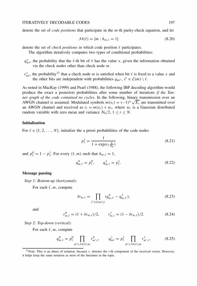
ITERATIVELY DECODABLE CODES 197
denote the set of code positions that participate in the m-th parity-check equation, and let
M(�) = {m : hm,� = 1} (8.20)
denote the set of check positions in which code position � participates.The algorithm iteratively computes two types of conditional probabilities:
qxm�, the probability that the �-th bit of v has the value x, given the information obtained
via the check nodes other than check node m.
rxm�, the probability12 that a check node m is satisfied when bit � is fixed to a value x and
the other bits are independent with probabilities qm�′ , �′ ∈ L(m) \ �.
As noted in MacKay (1999) and Pearl (1988), the following IBP decoding algorithm wouldproduce the exact a posteriori probabilities after some number of iterations if the Tan-ner graph of the code contained no cycles. In the following, binary transmission over anAWGN channel is assumed. Modulated symbols m(vi) = (−1)vi
√Es are transmitted over
an AWGN channel and received as ri = m(vi) + wi , where wi is a Gaussian distributedrandom variable with zero mean and variance N0/2, 1 ≤ i ≤ N .
Initialization
For � ∈ {1, 2, . . . , N}, initialize the a priori probabilities of the code nodes
p1� = 1
1 + exp(r�4
N0)
(8.21)
and p0� = 1 − p1
� . For every (�, m) such that hm,� = 1,
q0m,� = p0
�, q1m,� = p1
� . (8.22)
Message passing
Step 1: Bottom-up (horizontal):
For each �, m, compute
δrm,� =∏
�′∈L(m)\�(q0
m,�′ − q1m,�′), (8.23)
andr0m,� = (1 + δrm,�)/2, r1
m,� = (1 − δrm,�)/2. (8.24)
Step 2: Top-down (vertical):
For each �, m, compute
q0m,� = p0
�
∏m′∈M(�)\m
r0m′,�, q1
m� = p1�
∏m′∈M(�)\m
r1m′,�, (8.25)
12Note: This is an abuse of notation, because ri denotes the i-th component of the received vector. However,it helps keep the same notation as most of the literature in the topic.
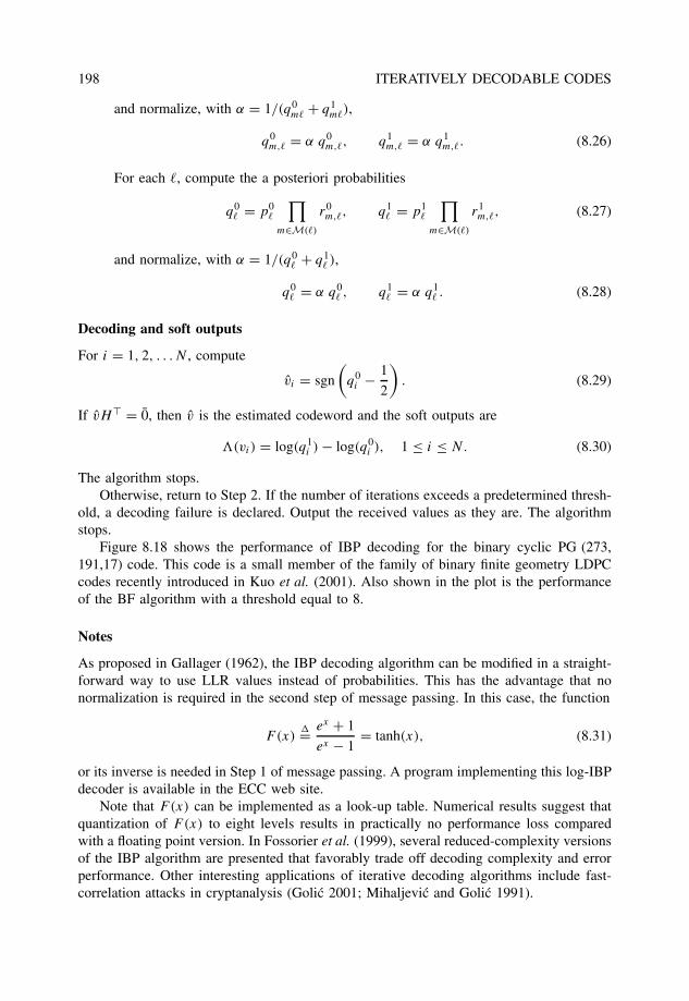
198 ITERATIVELY DECODABLE CODES
and normalize, with α = 1/(q0m� + q1
m�),
q0m,� = α q0
m,�, q1m,� = α q1
m,�. (8.26)
For each �, compute the a posteriori probabilities
q0� = p0
�
∏m∈M(�)
r0m,�, q1
� = p1�
∏m∈M(�)
r1m,�, (8.27)
and normalize, with α = 1/(q0� + q1
� ),
q0� = α q0
� , q1� = α q1
� . (8.28)
Decoding and soft outputs
For i = 1, 2, . . . N , compute
vi = sgn
(q0
i − 1
2
). (8.29)
If vH = 0, then v is the estimated codeword and the soft outputs are
�(vi) = log(q1i ) − log(q0
i ), 1 ≤ i ≤ N. (8.30)
The algorithm stops.Otherwise, return to Step 2. If the number of iterations exceeds a predetermined thresh-
old, a decoding failure is declared. Output the received values as they are. The algorithmstops.
Figure 8.18 shows the performance of IBP decoding for the binary cyclic PG (273,191,17) code. This code is a small member of the family of binary finite geometry LDPCcodes recently introduced in Kuo et al. (2001). Also shown in the plot is the performanceof the BF algorithm with a threshold equal to 8.
Notes
As proposed in Gallager (1962), the IBP decoding algorithm can be modified in a straight-forward way to use LLR values instead of probabilities. This has the advantage that nonormalization is required in the second step of message passing. In this case, the function
F(x)�= ex + 1
ex − 1= tanh(x), (8.31)
or its inverse is needed in Step 1 of message passing. A program implementing this log-IBPdecoder is available in the ECC web site.
Note that F(x) can be implemented as a look-up table. Numerical results suggest thatquantization of F(x) to eight levels results in practically no performance loss comparedwith a floating point version. In Fossorier et al. (1999), several reduced-complexity versionsof the IBP algorithm are presented that favorably trade off decoding complexity and errorperformance. Other interesting applications of iterative decoding algorithms include fast-correlation attacks in cryptanalysis (Golic 2001; Mihaljevic and Golic 1991).
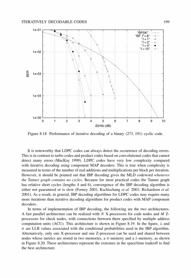
ITERATIVELY DECODABLE CODES 199
1e-05
1e-04
1e-03
1e-02
1e-01
0 1 2 3 4 5 6 7 8 9 10
BE
R
Eb/No (dB)
"BPSK""BF T = 8"
"I = 1""I = 2""I = 4"
"I = 10"
Figure 8.18 Performance of iterative decoding of a binary (273, 191) cyclic code.
It is noteworthy that LDPC codes can always detect the occurrence of decoding errors.This is in contrast to turbo codes and product codes based on convolutional codes that cannotdetect many errors (MacKay 1999). LDPC codes have very low complexity comparedwith iterative decoding using component MAP decoders. This is true when complexity ismeasured in terms of the number of real additions and multiplications per block per iteration.However, it should be pointed out that IBP decoding gives the MLD codeword wheneverthe Tanner graph contains no cycles. Because for most practical codes the Tanner graphhas relative short cycles (lengths 4 and 6), convergence of the IBP decoding algorithm iseither not guaranteed or is slow (Forney 2001; Kschischang et al. 2001; Richardson et al.2001). As a result, in general, IBP decoding algorithms for LDPC codes may require manymore iterations than iterative decoding algorithms for product codes with MAP componentdecoders.
In terms of implementation of IBP decoding, the following are the two architectures.A fast parallel architecture can be realized with N X-processors for code nodes and M Z-processors for check nodes, with connections between them specified by multiple addresscomputation units (ACU). This architecture is shown in Figure 8.19. In the figure, λ andπ are LLR values associated with the conditional probabilities used in the IBP algorithm.Alternatively, only one X-processor and one Z-processor can be used and shared betweennodes whose metrics are stored in two memories, a π -memory and a λ-memory, as shownin Figure 8.20. These architectures represent the extremes in the space/time tradeoff to findthe best architecture.
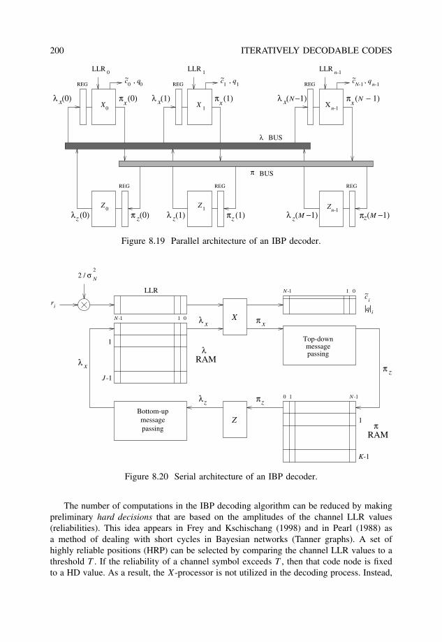
200 ITERATIVELY DECODABLE CODES
λ (0)x λ (1)xπ (0) π (1)X0 X 1 X
n-1
LLR 0 LLR 1 LLRn-1
0c , q 0 11 N-1c , q n-1
~~~
0Z Z Z1 n-1
xxx x
λ (0)z π (0) λ (1)z π (1) ( −1)Mλ ( −1)
π ( − 1)N
z z zz
REG REG REG
REGREGREG
BUS
BUSλ
π
c , q
N
M
λ ( −1)
π
Figure 8.19 Parallel architecture of an IBP decoder.
Bottom-upmessagepassing
Top-downmessagepassing
Z
X
0N -1 1LLR
ri
2 / σN
2
λz πz
λ x π x
c ~i
|q| i
π zλ x
1
J -1
1
K-1
N -10 1
01N -1
λRAM
RAMπ
Figure 8.20 Serial architecture of an IBP decoder.
The number of computations in the IBP decoding algorithm can be reduced by makingpreliminary hard decisions that are based on the amplitudes of the channel LLR values(reliabilities). This idea appears in Frey and Kschischang (1998) and in Pearl (1988) asa method of dealing with short cycles in Bayesian networks (Tanner graphs). A set ofhighly reliable positions (HRP) can be selected by comparing the channel LLR values to athreshold T . If the reliability of a channel symbol exceeds T , then that code node is fixedto a HD value. As a result, the X-processor is not utilized in the decoding process. Instead,
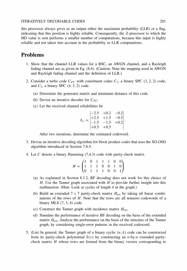
ITERATIVELY DECODABLE CODES 201
this processor always gives as an output either the maximum probability (LLR) or a flag,indicating that this position is highly reliable. Consequently, the Z-processor to which theHD value is sent performs a smaller number of computations, because this input is highlyreliable and not taken into account in the probability or LLR computations.
Problems
1. Show that the channel LLR values for a BSC, an AWGN channel, and a Rayleighfading channel are as given in Eq. (8.4). (Caution: Note the mapping used in AWGNand Rayleigh fading channel and the definition of LLR.)
2. Consider a turbo code CPC with constituent codes C1, a binary SPC (3, 2, 2) code,and C2, a binary SPC (4, 3, 2) code.
(a) Determine the generator matrix and minimum distance of this code.
(b) Devise an iterative decoder for CPC .
(c) Let the received channel reliabilities be
�c =
∣∣∣∣∣∣∣∣−2.5 +0.2 −0.2+2.5 +1.5 −0.5−1.5 −1.5 +0.2+0.5 +0.5
∣∣∣∣∣∣∣∣.
After two iterations, determine the estimated codeword.
3. Devise an iterative decoding algorithm for block product codes that uses the SO-OSDalgorithm introduced in Section 7.8.5.
4. Let C denote a binary Hamming (7,4,3) code with parity-check matrix
H =1 0 1 1 1 0 0
1 1 1 0 0 1 00 1 1 1 0 0 1
(a) As explained in Section 8.3.2, BF decoding does not work for this choice ofH . Use the Tanner graph associated with H to provide further insight into thismalfunction. (Hint: Look at cycles of length 4 in the graph.)
(b) Build an extended 7 × 7 parity-check matrix Hext by taking all linear combi-nations of the rows of H . Note that the rows are all nonzero codewords of abinary MLS (7, 3, 4) code.
(c) Construct the Tanner graph with incidence matrix Hext.
(d) Simulate the performance of iterative BF decoding on the basis of the extendedmatrix Hext. Analyze the performance on the basis of the structure of the Tannergraph, by considering single-error patterns in the received codeword.
5. (Lin) In general, the Tanner graph of a binary cyclic (n, k) code can be constructedfrom its parity-check polynomial h(x) by constructing an n-by-n extended parity-check matrix H whose rows are formed from the binary vectors corresponding to
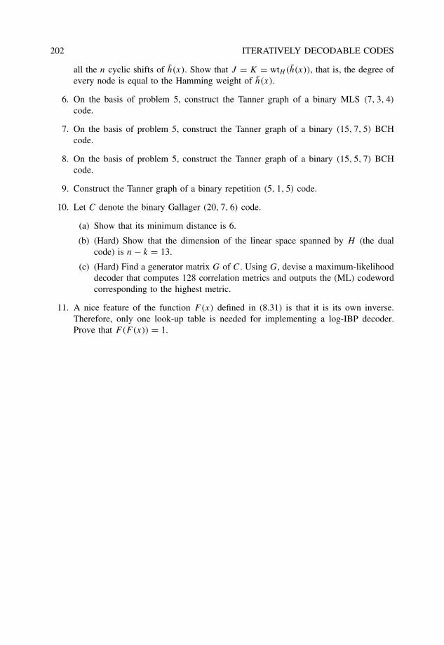
202 ITERATIVELY DECODABLE CODES
all the n cyclic shifts of h(x). Show that J = K = wtH (h(x)), that is, the degree ofevery node is equal to the Hamming weight of h(x).
6. On the basis of problem 5, construct the Tanner graph of a binary MLS (7, 3, 4)
code.
7. On the basis of problem 5, construct the Tanner graph of a binary (15, 7, 5) BCHcode.
8. On the basis of problem 5, construct the Tanner graph of a binary (15, 5, 7) BCHcode.
9. Construct the Tanner graph of a binary repetition (5, 1, 5) code.
10. Let C denote the binary Gallager (20, 7, 6) code.
(a) Show that its minimum distance is 6.
(b) (Hard) Show that the dimension of the linear space spanned by H (the dualcode) is n − k = 13.
(c) (Hard) Find a generator matrix G of C. Using G, devise a maximum-likelihooddecoder that computes 128 correlation metrics and outputs the (ML) codewordcorresponding to the highest metric.
11. A nice feature of the function F(x) defined in (8.31) is that it is its own inverse.Therefore, only one look-up table is needed for implementing a log-IBP decoder.Prove that F(F(x)) = 1.
9
Combining codes and digitalmodulation
In discussing SDD, attention was focused on binary transmission, that is, using two possibletransmitted symbols {−1, +1}. Let the Nyquist bandwidth of a transmission (or storage)signal be the rate Rs at which symbols are transmitted (or stored). For binary transmission,the two values of a bit, 0 and 1, are assigned to two values of the transmitted symbol, +1and −1, respectively. Therefore, Rs bits/second require a Nyquist bandwidth of Rs Hz. Thespectral efficiency µ of a binary transmission system equals 1 bit/sec/Hz (or 1 bit/symbol).Coded modulation is the joint design of error correcting codes and digital modulationformats to increase the bandwidth efficiency of a digital communication system.
9.1 MotivationSuppose an error correcting coding scheme is required to increase the reliability of thebinary transmission (or storage) system. Let Rc = k/n denote the rate of the code. Thenthe spectral efficiency is µ = Rc bps/Hz. Thus for a coded binary transmission system, aspectral efficiency µ ≤ 1 bps/Hz is achieved. This translates into a faster signaling rate orlarger bandwidth for the same bit rate. Equivalently, the bit rate has to be reduced by afactor of 1/Rs so as to keep the transmitted symbol rate or bandwidth constant.
Example 9.1.1 Assume that 56 kbps are desired to be transmitted over a channel. Therequired Nyquist bandwidth of an uncoded binary transmission system is 56 kHz. Suppose arate-1/2 convolutional code is used. Then, with binary transmission, the spectral efficiencyof the coded system is µ = 0.5 bps/Hz. The effect of µ in data rate and signaling rate isillustrated in Figure 9.1.
Increasing the bandwidth of the signal as in Figure 9.1 (a) is not a practical solutionsince typically the channel bandwidth is expensive (or limited, as in a telephone line).Decreasing the data rate (Figure 9.1 (b)) is a possible solution, but places a limit on thenumber of services or applications offered. In addition, the increased transmission delaymay not be acceptable (e.g., voice or video).
The Art of Error Correcting Coding, Second Edition Robert H. Morelos-Zaragoza 2006 John Wiley & Sons, Ltd. ISBN: 0-470-01558-6
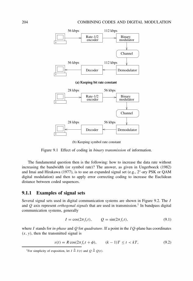
204 COMBINING CODES AND DIGITAL MODULATION
Binarymodulator
Demodulator
Channel
Rate-1/2encoder
Decoder
(a) Keeping bit rate constant
112 kbps56 kbps
112 kbps56 kbps
(a) Keeping bit rate constant
Binarymodulator
Demodulator
Channel
Rate-1/2encoder
Decoder
56 kbps28 kbps
56 kbps28 kbps
(b) Keeping symbol rate constant
Figure 9.1 Effect of coding in binary transmission of information.
The fundamental question then is the following: how to increase the data rate withoutincreasing the bandwidth (or symbol rate)? The answer, as given in Ungerboeck (1982)and Imai and Hirakawa (1977), is to use an expanded signal set (e.g., 2ν-ary PSK or QAMdigital modulation) and then to apply error correcting coding to increase the Euclideandistance between coded sequences.
9.1.1 Examples of signal sets
Several signal sets used in digital communication systems are shown in Figure 9.2. The I
and Q axis represent orthogonal signals that are used in transmission.1 In bandpass digitalcommunication systems, generally
I = cos(2πfct), Q = sin(2πfct), (9.1)
where I stands for in-phase and Q for quadrature. If a point in the IQ-plane has coordinates(x, y), then the transmitted signal is
s(t) = R cos(2πfct + φ), (k − 1)T ≤ t < kT , (9.2)
1For simplicity of exposition, let I�= I (t) and Q
�= Q(t).
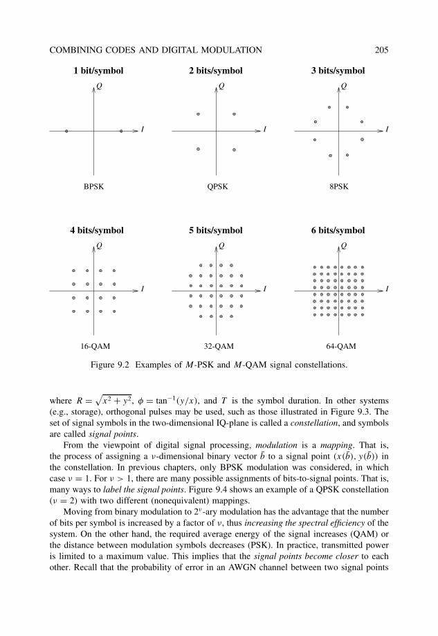
COMBINING CODES AND DIGITAL MODULATION 205
I
Q
I
Q
I
Q
2 bits/symbol 3 bits/symbol1 bit/symbol
I
Q
4 bits/symbol 6 bits/symbol5 bits/symbol
I
Q
I
Q
BPSK QPSK 8PSK
16-QAM 32-QAM 64-QAM
Figure 9.2 Examples of M-PSK and M-QAM signal constellations.
where R =√
x2 + y2, φ = tan−1(y/x), and T is the symbol duration. In other systems(e.g., storage), orthogonal pulses may be used, such as those illustrated in Figure 9.3. Theset of signal symbols in the two-dimensional IQ-plane is called a constellation, and symbolsare called signal points.
From the viewpoint of digital signal processing, modulation is a mapping. That is,the process of assigning a ν-dimensional binary vector b to a signal point (x(b), y(b)) inthe constellation. In previous chapters, only BPSK modulation was considered, in whichcase ν = 1. For ν > 1, there are many possible assignments of bits-to-signal points. That is,many ways to label the signal points. Figure 9.4 shows an example of a QPSK constellation(ν = 2) with two different (nonequivalent) mappings.
Moving from binary modulation to 2ν-ary modulation has the advantage that the numberof bits per symbol is increased by a factor of ν, thus increasing the spectral efficiency of thesystem. On the other hand, the required average energy of the signal increases (QAM) orthe distance between modulation symbols decreases (PSK). In practice, transmitted poweris limited to a maximum value. This implies that the signal points become closer to eachother. Recall that the probability of error in an AWGN channel between two signal points
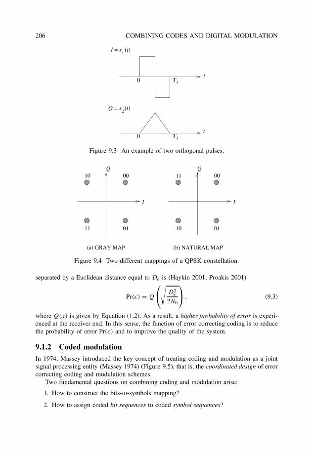
206 COMBINING CODES AND DIGITAL MODULATION
Ts
Ts
0
0
1
2
I = s (t)
Q = s (t)
t
t
Figure 9.3 An example of two orthogonal pulses.
I
Q
I
Q
01
0010
11
0011
10 01
(a) GRAY MAP (b) NATURAL MAP
Figure 9.4 Two different mappings of a QPSK constellation.
separated by a Euclidean distance equal to De is (Haykin 2001; Proakis 2001)
Pr(ε) = Q
√D2
e
2N0
, (9.3)
where Q(x) is given by Equation (1.2). As a result, a higher probability of error is experi-enced at the receiver end. In this sense, the function of error correcting coding is to reducethe probability of error Pr(ε) and to improve the quality of the system.
9.1.2 Coded modulationIn 1974, Massey introduced the key concept of treating coding and modulation as a jointsignal processing entity (Massey 1974) (Figure 9.5), that is, the coordinated design of errorcorrecting coding and modulation schemes.
Two fundamental questions on combining coding and modulation arise:
1. How to construct the bits-to-symbols mapping?
2. How to assign coded bit sequences to coded symbol sequences?

COMBINING CODES AND DIGITAL MODULATION 207
Source Encoder Modulator
Channel
DemodulatorDecoderSink
Combine codingand modulation
(Massey, 1974)
Figure 9.5 The idea of joint coding and modulation.
Two basic approaches were proposed in the 1970s to design coded modulation systems:
1. Trellis-Coded Modulation (TCM) (Ungerboeck 1982)
Apply a natural mapping of bits to signals, through set partitioning. Given an under-lying finite-state machine, assign symbol sequences to trellis paths. Perform Viterbidecoding at the receiver.
2. Multilevel Coded Modulation (MCM) (Imai and Hirakawa 1977)
Apply a mapping of codewords to bit positions, through a binary partition. For 2ν-arymodulation, use ν error correcting codes, one per label bit. Perform multistage decod-ing at the receiver.
In both TCM (Trellis Coded Modulation) and MCM (Multilevel Coded Modulation), thebasic idea is to expand the constellation to obtain the redundancy needed for error correct-ing coding, and then to use coding to increase the minimum Euclidean distance betweensequences of modulated signals.
9.1.3 Distance considerations
To illustrate how error correcting codes and digital modulation can be combined and theconsequent increase in the minimum distance between signal sequences from an expandedsignal constellation, consider the following.
Example 9.1.2 A block-coded QPSK modulation scheme is shown in Figure 9.6. Codewordsof the extended Hamming (8, 4, 4) code are divided into four pairs of symbols and mappedto QPSK signal points with Gray mapping. A nice feature of Gray labeling of QPSK points isthat the squared Euclidean distance between points is equal to twice the Hamming distancebetween their labels. As a result, a block-coded modulation scheme with µ = 1 bit/symboland a minimum squared Euclidean distance (MSED) D2
min = 8 is obtained. An uncodedsystem with the same spectral efficiency is BPSK, which has an MSED D2
unc = 4. It followsthat the asymptotic coding gain of this scheme is
G = 10 log10
(D2
min
D2unc
)= 3 dB. (9.4)
Over an AWGN channel, this coded QPSK modulation requires half the power of uncodedBPSK modulation, to achieve the same probability of error P (ε). Figure 9.7 shows simula-tion results of this scheme.
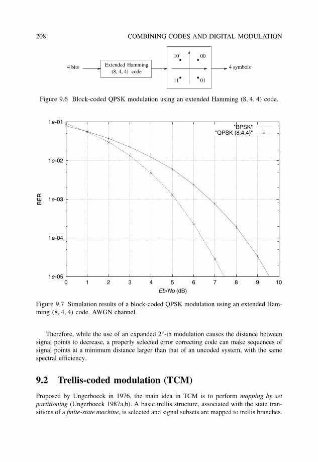
208 COMBINING CODES AND DIGITAL MODULATION
00
0111
10
Extended Hamming 4 symbols4 bits(8, 4, 4) code
Figure 9.6 Block-coded QPSK modulation using an extended Hamming (8, 4, 4) code.
1e-05
1e-04
1e-03
1e-02
1e-01
0 1 2 3 4 5 6 7 8 9 10
BE
R
Eb/No (dB)
"BPSK""QPSK (8,4,4)"
Figure 9.7 Simulation results of a block-coded QPSK modulation using an extended Ham-ming (8, 4, 4) code. AWGN channel.
Therefore, while the use of an expanded 2ν-th modulation causes the distance betweensignal points to decrease, a properly selected error correcting code can make sequences ofsignal points at a minimum distance larger than that of an uncoded system, with the samespectral efficiency.
9.2 Trellis-coded modulation (TCM)
Proposed by Ungerboeck in 1976, the main idea in TCM is to perform mapping by setpartitioning (Ungerboeck 1987a,b). A basic trellis structure, associated with the state tran-sitions of a finite-state machine, is selected and signal subsets are mapped to trellis branches.
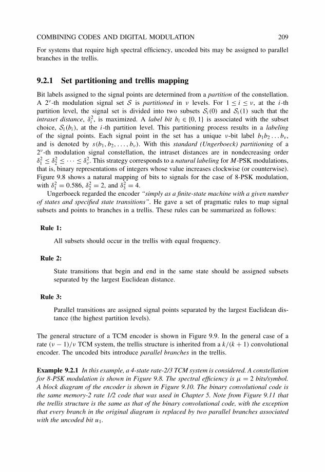
COMBINING CODES AND DIGITAL MODULATION 209
For systems that require high spectral efficiency, uncoded bits may be assigned to parallelbranches in the trellis.
9.2.1 Set partitioning and trellis mapping
Bit labels assigned to the signal points are determined from a partition of the constellation.A 2ν-th modulation signal set S is partitioned in ν levels. For 1 ≤ i ≤ ν, at the i-thpartition level, the signal set is divided into two subsets Si (0) and Si (1) such that theintraset distance, δ2
i , is maximized. A label bit bi ∈ {0, 1} is associated with the subsetchoice, Si (bi), at the i-th partition level. This partitioning process results in a labelingof the signal points. Each signal point in the set has a unique ν-bit label b1b2 . . . bν ,and is denoted by s(b1, b2, . . . , bν). With this standard (Ungerboeck) partitioning of a2ν-th modulation signal constellation, the intraset distances are in nondecreasing orderδ2
1 ≤ δ22 ≤ · · · ≤ δ2
ν . This strategy corresponds to a natural labeling for M-PSK modulations,that is, binary representations of integers whose value increases clockwise (or counterwise).Figure 9.8 shows a natural mapping of bits to signals for the case of 8-PSK modulation,with δ2
1 = 0.586, δ22 = 2, and δ2
3 = 4.Ungerboeck regarded the encoder “simply as a finite-state machine with a given number
of states and specified state transitions”. He gave a set of pragmatic rules to map signalsubsets and points to branches in a trellis. These rules can be summarized as follows:
Rule 1:
All subsets should occur in the trellis with equal frequency.
Rule 2:
State transitions that begin and end in the same state should be assigned subsetsseparated by the largest Euclidean distance.
Rule 3:
Parallel transitions are assigned signal points separated by the largest Euclidean dis-tance (the highest partition levels).
The general structure of a TCM encoder is shown in Figure 9.9. In the general case of arate (ν − 1)/ν TCM system, the trellis structure is inherited from a k/(k + 1) convolutionalencoder. The uncoded bits introduce parallel branches in the trellis.
Example 9.2.1 In this example, a 4-state rate-2/3 TCM system is considered. A constellationfor 8-PSK modulation is shown in Figure 9.8. The spectral efficiency is µ = 2 bits/symbol.A block diagram of the encoder is shown in Figure 9.10. The binary convolutional code isthe same memory-2 rate 1/2 code that was used in Chapter 5. Note from Figure 9.11 thatthe trellis structure is the same as that of the binary convolutional code, with the exceptionthat every branch in the original diagram is replaced by two parallel branches associatedwith the uncoded bit u1.
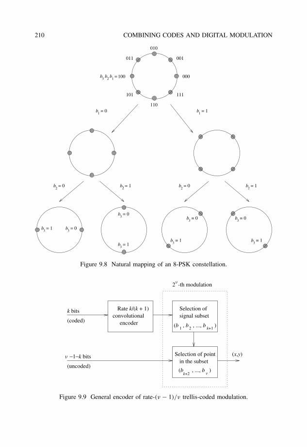
210 COMBINING CODES AND DIGITAL MODULATION
b = 02
b = 022
000100
1b =
1b = 0
3 12b b b =
b = 12
b = 1
010
110
001011
111101
1
b = 13
b = 03
b = 03
b = 13
b = 13
b = 03
b = 03
b = 13
Figure 9.8 Natural mapping of an 8-PSK constellation.
(b , ..., b )k+2 n
k+12(b , b , ..., b )
1
convolutionalencoder
Rate k/(k + 1)k bits
(coded)
(uncoded)
(x,y)
Selection ofsignal subset
Selection of pointin the subset
2 -th modulationn
−1−k bitsn
Figure 9.9 General encoder of rate-(ν − 1)/ν trellis-coded modulation.
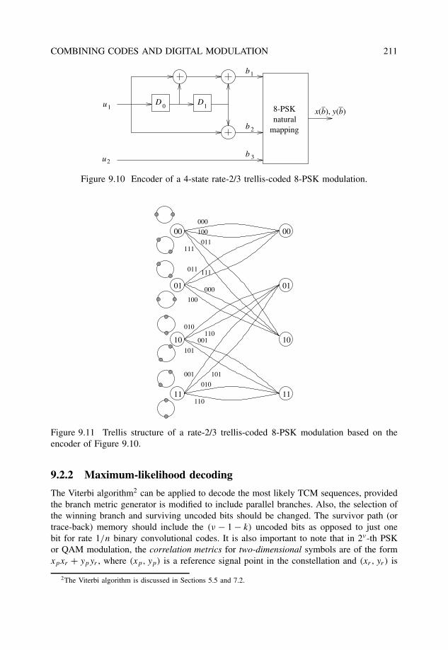
COMBINING CODES AND DIGITAL MODULATION 211
0D D
1u
u
b
b
b
1
2
3
8-PSKnatural
mapping
x(b), y(b)1
2
Figure 9.10 Encoder of a 4-state rate-2/3 trellis-coded 8-PSK modulation.
11
00 00
01 01
10 10
000
100
011111
000
100
011 111
010110
001
101
11
001 101
010
110
Figure 9.11 Trellis structure of a rate-2/3 trellis-coded 8-PSK modulation based on theencoder of Figure 9.10.
9.2.2 Maximum-likelihood decoding
The Viterbi algorithm2 can be applied to decode the most likely TCM sequences, providedthe branch metric generator is modified to include parallel branches. Also, the selection ofthe winning branch and surviving uncoded bits should be changed. The survivor path (ortrace-back) memory should include the (ν − 1 − k) uncoded bits as opposed to just onebit for rate 1/n binary convolutional codes. It is also important to note that in 2ν-th PSKor QAM modulation, the correlation metrics for two-dimensional symbols are of the formxpxr + ypyr , where (xp, yp) is a reference signal point in the constellation and (xr, yr ) is
2The Viterbi algorithm is discussed in Sections 5.5 and 7.2.
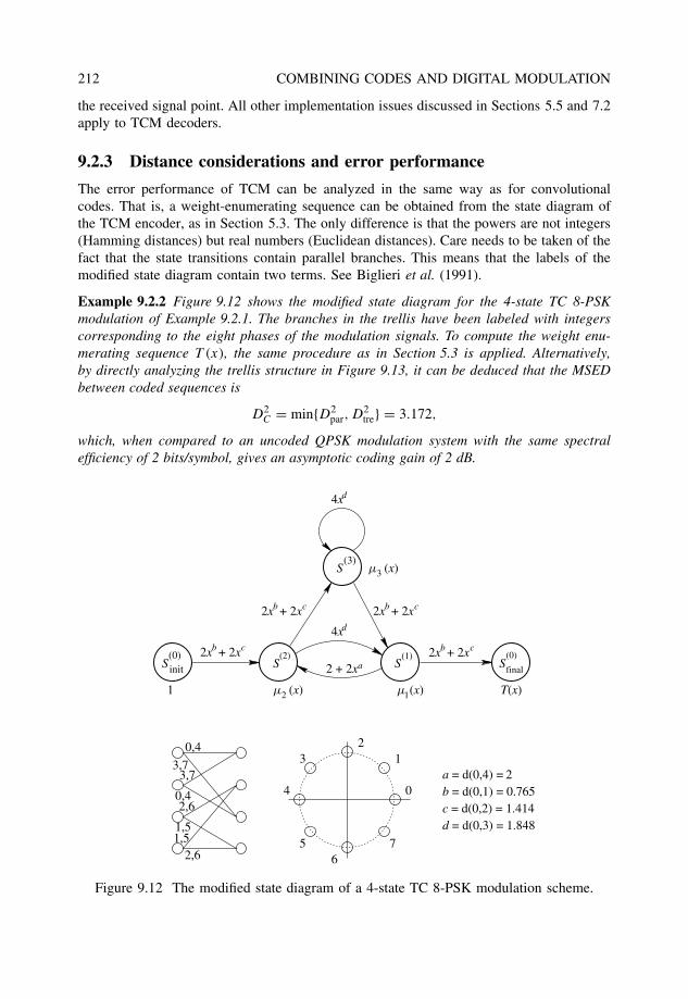
212 COMBINING CODES AND DIGITAL MODULATION
the received signal point. All other implementation issues discussed in Sections 5.5 and 7.2apply to TCM decoders.
9.2.3 Distance considerations and error performance
The error performance of TCM can be analyzed in the same way as for convolutionalcodes. That is, a weight-enumerating sequence can be obtained from the state diagram ofthe TCM encoder, as in Section 5.3. The only difference is that the powers are not integers(Hamming distances) but real numbers (Euclidean distances). Care needs to be taken of thefact that the state transitions contain parallel branches. This means that the labels of themodified state diagram contain two terms. See Biglieri et al. (1991).
Example 9.2.2 Figure 9.12 shows the modified state diagram for the 4-state TC 8-PSKmodulation of Example 9.2.1. The branches in the trellis have been labeled with integerscorresponding to the eight phases of the modulation signals. To compute the weight enu-merating sequence T (x), the same procedure as in Section 5.3 is applied. Alternatively,by directly analyzing the trellis structure in Figure 9.13, it can be deduced that the MSEDbetween coded sequences is
D2C = min{D2
par, D2tre} = 3.172,
which, when compared to an uncoded QPSK modulation system with the same spectralefficiency of 2 bits/symbol, gives an asymptotic coding gain of 2 dB.
1,5
0,4
3,7
0,4
1,5
2,6
3,7
2,6
2
4
3 1
56
0
7
a = d(0,4) = 2b = d(0,1) = 0.765c = d(0,2) = 1.414d = d(0,3) = 1.848
S
S S
m m
m
T(x)
S
1
init(0) (2) (1)
(3)3
2 1
Sfinal
(0)
(x)
(x)
(x)
4x
2 + 2xa
2x + 2x
d
4xd
b 2x + 2xbc
2x + 2xb c
c
2x + 2xb c
Figure 9.12 The modified state diagram of a 4-state TC 8-PSK modulation scheme.
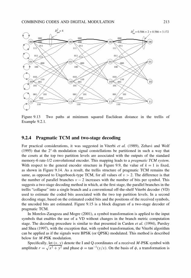
COMBINING CODES AND DIGITAL MODULATION 213
11 11 11
00
01
10
11
00
01
10
000
100
011111
000
100
011 111
010110
001
101
001 101
010
110
00
01
10
000
100
011111
000
100
011 111
010110
001
101
001 101
010
110
00
01
10
000
100
011111
000
100
011 111
010110
001
101
001 101
010
110
D = 4par2 2D = 0.586 + 2 + 0.586 = 3.172
tre
Figure 9.13 Two paths at minimum squared Euclidean distance in the trellis ofExample 9.2.1.
9.2.4 Pragmatic TCM and two-stage decoding
For practical considerations, it was suggested in Viterbi et al. (1989), Zehavi and Wolf(1995) that the 2ν-th modulation signal constellations be partitioned in such a way thatthe cosets at the top two partition levels are associated with the outputs of the standardmemory-6 rate-1/2 convolutional encoder. This mapping leads to a pragmatic TCM system.With respect to the general encoder structure in Figure 9.9, the value of k = 1 is fixed,as shown in Figure 9.14. As a result, the trellis structure of pragmatic TCM remains thesame, as opposed to Ungerboeck-type TCM, for all values of ν > 2. The difference is thatthe number of parallel branches ν − 2 increases with the number of bits per symbol. Thissuggests a two-stage decoding method in which, at the first stage, the parallel branches in thetrellis “collapse” into a single branch and a conventional off-the-shelf Viterbi decoder (VD)used to estimate the coded bits associated with the two top partition levels. In a seconddecoding stage, based on the estimated coded bits and the positions of the received symbols,the uncoded bits are estimated. Figure 9.15 is a block diagram of a two-stage decoder ofpragmatic TCM.
In Morelos-Zaragoza and Mogre (2001), a symbol transformation is applied to the inputsymbols that enables the use of a VD without changes in the branch metric computationstage. The decoding procedure is similar to that presented in Carden et al. (1994), Pursleyand Shea (1997), with the exception that, with symbol transformation, the Viterbi algorithmcan be applied as if the signals were BPSK (or QPSK) modulated. This method is describedbelow for M-PSK modulation.
Specifically, let (x, y) denote the I and Q coordinates of a received M-PSK symbol withamplitude r =
√x2 + y2 and phase φ = tan−1(y/x). On the basis of φ, a transformation is
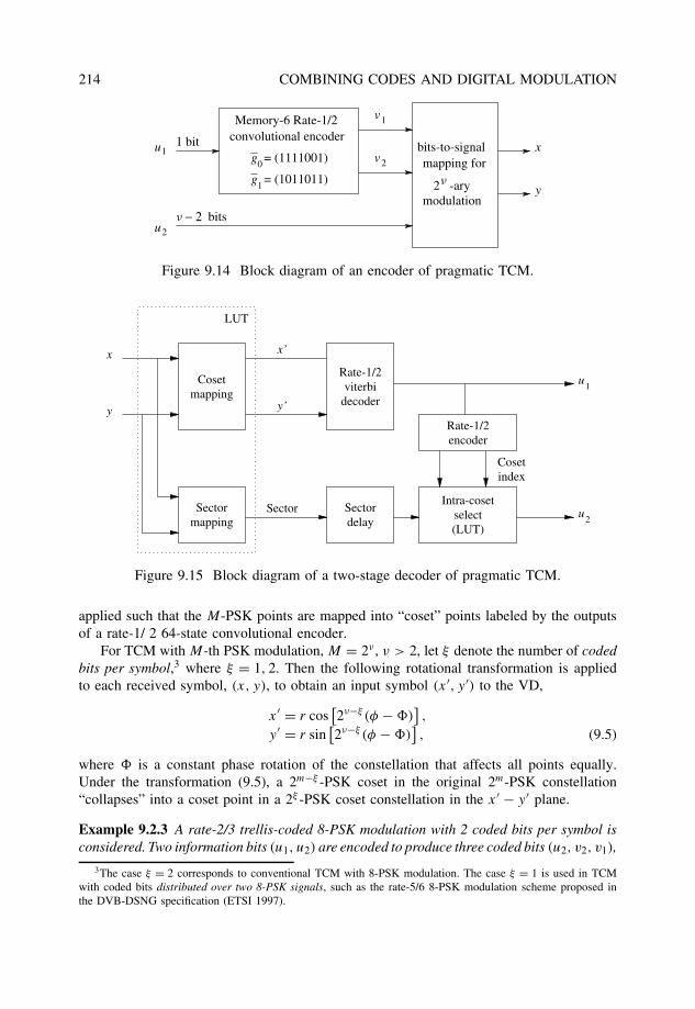
214 COMBINING CODES AND DIGITAL MODULATION
2 -aryn
Memory-6 Rate-1/2convolutional encoder
g = (1111001)0
1g = (1011011)
1 bit
n − 2 bits
bits-to-signalmapping for
modulation
x
y
u
u
v
v
2
1
1
2
Figure 9.14 Block diagram of an encoder of pragmatic TCM.
Sectordelay
Rate-1/2viterbi
decoder
Cosetmapping
x
y
x’
y’
LUT
Sectormapping
Sector
Rate-1/2encoder
Intra-cosetselect(LUT)
Cosetindex
u
u
1
2
Figure 9.15 Block diagram of a two-stage decoder of pragmatic TCM.
applied such that the M-PSK points are mapped into “coset” points labeled by the outputsof a rate-1/ 2 64-state convolutional encoder.
For TCM with M-th PSK modulation, M = 2ν , ν > 2, let ξ denote the number of codedbits per symbol,3 where ξ = 1, 2. Then the following rotational transformation is appliedto each received symbol, (x, y), to obtain an input symbol (x ′, y ′) to the VD,
x ′ = r cos[2ν−ξ (φ − �)
],
y ′ = r sin[2ν−ξ (φ − �)
], (9.5)
where � is a constant phase rotation of the constellation that affects all points equally.Under the transformation (9.5), a 2m−ξ -PSK coset in the original 2m-PSK constellation“collapses” into a coset point in a 2ξ -PSK coset constellation in the x ′ − y ′ plane.
Example 9.2.3 A rate-2/3 trellis-coded 8-PSK modulation with 2 coded bits per symbol isconsidered. Two information bits (u1, u2) are encoded to produce three coded bits (u2, v2, v1),
3The case ξ = 2 corresponds to conventional TCM with 8-PSK modulation. The case ξ = 1 is used in TCMwith coded bits distributed over two 8-PSK signals, such as the rate-5/6 8-PSK modulation scheme proposed inthe DVB-DSNG specification (ETSI 1997).
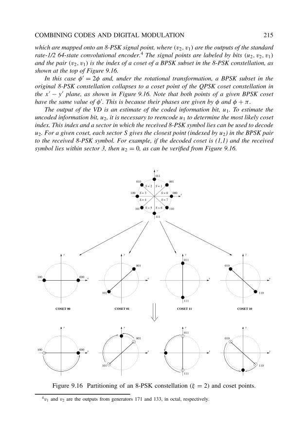
COMBINING CODES AND DIGITAL MODULATION 215
which are mapped onto an 8-PSK signal point, where (v2, v1) are the outputs of the standardrate-1/2 64-state convolutional encoder.4 The signal points are labeled by bits (u2, v2, v1)
and the pair (v2, v1) is the index of a coset of a BPSK subset in the 8-PSK constellation, asshown at the top of Figure 9.16.
In this case φ′ = 2φ and, under the rotational transformation, a BPSK subset in theoriginal 8-PSK constellation collapses to a coset point of the QPSK coset constellation inthe x ′ − y ′ plane, as shown in Figure 9.16. Note that both points of a given BPSK cosethave the same value of φ′. This is because their phases are given by φ and φ + π .
The output of the VD is an estimate of the coded information bit, u1. To estimate theuncoded information bit, u2, it is necessary to reencode u1 to determine the most likely cosetindex. This index and a sector in which the received 8-PSK symbol lies can be used to decodeu2. For a given coset, each sector S gives the closest point (indexed by u2) in the BPSK pairto the received 8-PSK symbol. For example, if the decoded coset is (1,1) and the receivedsymbol lies within sector 3, then u2 = 0, as can be verified from Figure 9.16.
001
000
011
010
111
100 x
y
S = 0
S = 1S = 2
S = 3
S = 4
S = 5 S = 6
S = 7
101 110
000100 x
y
001
x
y
011
111
x
y
010
x
y
101 110
000100 x
y
001
x
y
011
111
x
y
010
x
y
101 110
COSET 00 COSET 01 COSET 11 COSET 10
Figure 9.16 Partitioning of an 8-PSK constellation (ξ = 2) and coset points.
4v1 and v2 are the outputs from generators 171 and 133, in octal, respectively.
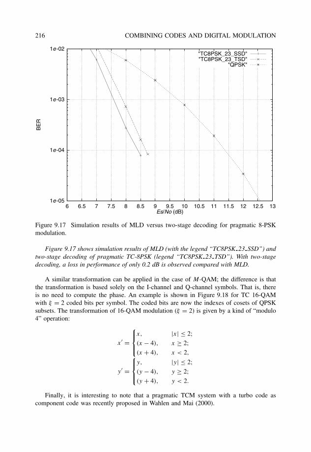
216 COMBINING CODES AND DIGITAL MODULATION
1e-05
1e-04
1e-03
1e-02
6 6.5 7 7.5 8 8.5 9 9.5 10 10.5 11 11.5 12 12.5 13
BE
R
Es/No (dB)
"TC8PSK_23_SSD""TC8PSK_23_TSD"
"QPSK"
Figure 9.17 Simulation results of MLD versus two-stage decoding for pragmatic 8-PSKmodulation.
Figure 9.17 shows simulation results of MLD (with the legend “TC8PSK 23 SSD”) andtwo-stage decoding of pragmatic TC-8PSK (legend “TC8PSK 23 TSD”). With two-stagedecoding, a loss in performance of only 0.2 dB is observed compared with MLD.
A similar transformation can be applied in the case of M-QAM; the difference is thatthe transformation is based solely on the I-channel and Q-channel symbols. That is, thereis no need to compute the phase. An example is shown in Figure 9.18 for TC 16-QAMwith ξ = 2 coded bits per symbol. The coded bits are now the indexes of cosets of QPSKsubsets. The transformation of 16-QAM modulation (ξ = 2) is given by a kind of “modulo4” operation:
x ′ =
x, |x| ≤ 2;(x − 4), x ≥ 2;(x + 4), x < 2,
y ′ =
y, |y| ≤ 2;(y − 4), y ≥ 2;(y + 4), y < 2.
Finally, it is interesting to note that a pragmatic TCM system with a turbo code ascomponent code was recently proposed in Wahlen and Mai (2000).
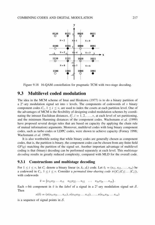
COMBINING CODES AND DIGITAL MODULATION 217
x
y
00110111
1111 1011
00100110
1110 1010
00010101
1101 1001
00000100
1100 1000
1
3
–1–3
–3
–1
1 3
S = 0S = 1S = 2
S = 3S = 4S = 5
S = 6S = 7S = 8
Figure 9.18 16-QAM constellation for pragmatic TCM with two-stage decoding.
9.3 Multilevel coded modulationThe idea in the MCM scheme of Imai and Hirakawa (1977) is to do a binary partition ofa 2ν-ary modulation signal set into ν levels. The components of codewords of ν binarycomponent codes Ci , 1 ≤ i ≤ ν, are used to index the cosets at each partition level. One ofthe advantages of MCM is the flexibility of designing coded modulation schemes by coordi-nating the intraset Euclidean distances, δ2
i , i = 1, 2, . . . , ν, at each level of set partitioning,and the minimum Hamming distances of the component codes. Wachsmann et al. (1999)have proposed several design rules that are based on capacity (by applying the chain ruleof mutual information) arguments. Moreover, multilevel codes with long binary componentcodes, such as turbo codes or LDPC codes, were shown to achieve capacity (Forney 1998;Wachsmann et al. 1999).
It is also worthwhile noting that while binary codes are generally chosen as componentcodes, that is, the partition is binary, the component codes can be chosen from any finite fieldGF(q) matching the partition of the signal set. Another important advantage of multilevelcoding is that (binary) decoding can be performed separately at each level. This multistagedecoding results in greatly reduced complexity, compared with MLD for the overall code.
9.3.1 Constructions and multistage decodingFor 1 ≤ i ≤ ν, let Ci denote a binary linear (n, ki, di) code. Let vi = (vi1, vi2, . . . , vin) bea codeword in Ci , 1 ≤ i ≤ ν. Consider a permuted time-sharing code π(|C1|C2| . . . |Cν |),with codewords
v = (v11v21 . . . vν1 v12v22 . . . vν2 . . . v1nv2n . . . vνn
).
Each ν-bit component in v is the label of a signal in a 2ν-ary modulation signal set S.Then
s(v) = (s(v11v21 . . . vν1), s(v12v22 . . . vν2), . . . , s(v1nv2n . . . vνn)
is a sequence of signal points in S.
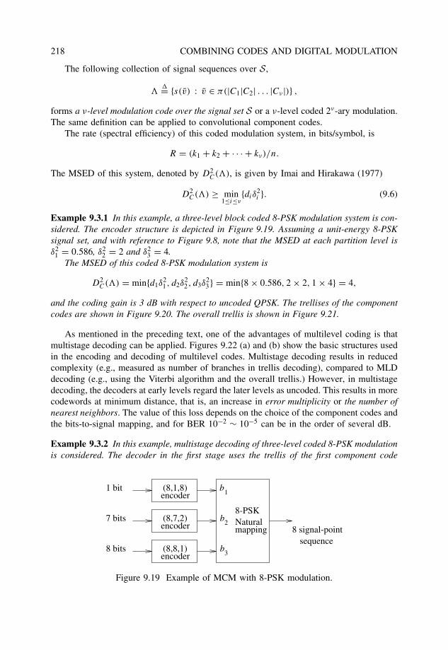
218 COMBINING CODES AND DIGITAL MODULATION
The following collection of signal sequences over S,
�= {s(v) : v ∈ π(|C1|C2| . . . |Cν |)} ,
forms a ν-level modulation code over the signal set S or a ν-level coded 2ν-ary modulation.The same definition can be applied to convolutional component codes.
The rate (spectral efficiency) of this coded modulation system, in bits/symbol, is
R = (k1 + k2 + · · · + kν)/n.
The MSED of this system, denoted by D2C(), is given by Imai and Hirakawa (1977)
D2C() ≥ min
1≤i≤ν{diδ
2i }. (9.6)
Example 9.3.1 In this example, a three-level block coded 8-PSK modulation system is con-sidered. The encoder structure is depicted in Figure 9.19. Assuming a unit-energy 8-PSKsignal set, and with reference to Figure 9.8, note that the MSED at each partition level isδ2
1 = 0.586, δ22 = 2 and δ2
3 = 4.The MSED of this coded 8-PSK modulation system is
D2C() = min{d1δ
21, d2δ
22, d3δ
23} = min{8 × 0.586, 2 × 2, 1 × 4} = 4,
and the coding gain is 3 dB with respect to uncoded QPSK. The trellises of the componentcodes are shown in Figure 9.20. The overall trellis is shown in Figure 9.21.
As mentioned in the preceding text, one of the advantages of multilevel coding is thatmultistage decoding can be applied. Figures 9.22 (a) and (b) show the basic structures usedin the encoding and decoding of multilevel codes. Multistage decoding results in reducedcomplexity (e.g., measured as number of branches in trellis decoding), compared to MLDdecoding (e.g., using the Viterbi algorithm and the overall trellis.) However, in multistagedecoding, the decoders at early levels regard the later levels as uncoded. This results in morecodewords at minimum distance, that is, an increase in error multiplicity or the number ofnearest neighbors. The value of this loss depends on the choice of the component codes andthe bits-to-signal mapping, and for BER 10−2 ∼ 10−5 can be in the order of several dB.
Example 9.3.2 In this example, multistage decoding of three-level coded 8-PSK modulationis considered. The decoder in the first stage uses the trellis of the first component code
(8,1,8)
(8,7,2)
encoder
encoder
encoder(8,8,1)
b
b3
2
b1
sequence8 signal-point
7 bits
1 bit
8 bits
Naturalmapping
8-PSK
Figure 9.19 Example of MCM with 8-PSK modulation.
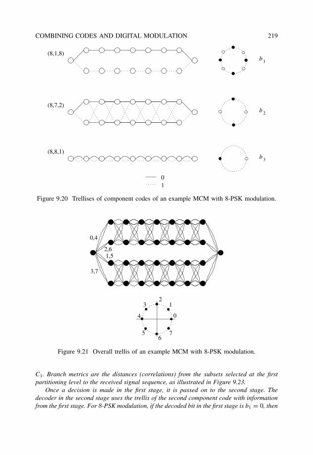
COMBINING CODES AND DIGITAL MODULATION 219
1
2
3
01
(8,1,8)
(8,7,2)
(8,8,1)
b
b
b
Figure 9.20 Trellises of component codes of an example MCM with 8-PSK modulation.
0
12
3
4
56
7
0,4
2,61,5
3,7
Figure 9.21 Overall trellis of an example MCM with 8-PSK modulation.
C1. Branch metrics are the distances (correlations) from the subsets selected at the firstpartitioning level to the received signal sequence, as illustrated in Figure 9.23.
Once a decision is made in the first stage, it is passed on to the second stage. Thedecoder in the second stage uses the trellis of the second component code with informationfrom the first stage. For 8-PSK modulation, if the decoded bit in the first stage is b1 = 0, then
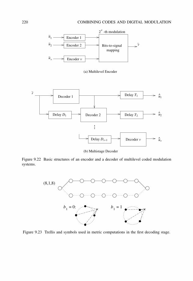
220 COMBINING CODES AND DIGITAL MODULATION
v
Delay Dn−1
Decoder 1
Decoder 2
Decoder n
Delay D1
Delay T1
Delay T2
un
u2
u1^
^
^
(b) Multistage Decoder
r
Encoder 1
Encoder 2
2 -th modulationn
(a) Multilevel Encoder
Encoder n
u
u
u
1
2
n
mappingBits-to-signal
...
Figure 9.22 Basic structures of an encoder and a decoder of multilevel coded modulationsystems.
(8,1,8)
1b = 0: 1b = 1
Figure 9.23 Trellis and symbols used in metric computations in the first decoding stage.
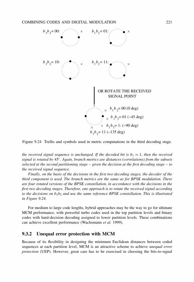
COMBINING CODES AND DIGITAL MODULATION 221
SIGNAL POINTOR ROTATE THE RECEIVED
b b = 01 (−45 deg)
b b = 11 (–135 deg)
1 2
1 2 1 2
1 2b b = 11:
b b = 00: b b = 01:
b b = 10:
b b = 1: (−90 deg)
b b = 00 (0 deg)
1
21
2
21
21
Figure 9.24 Trellis and symbols used in metric computations in the third decoding stage.
the received signal sequence is unchanged. If the decoded bit is b1 = 1, then the receivedsignal is rotated by 45◦. Again, branch metrics are distances (correlations) from the subsetsselected at the second partitioning stage – given the decision at the first decoding stage – tothe received signal sequence.
Finally, on the basis of the decisions in the first two decoding stages, the decoder of thethird component is used. The branch metrics are the same as for BPSK modulation. Thereare four rotated versions of the BPSK constellation, in accordance with the decisions in thefirst two decoding stages. Therefore, one approach is to rotate the received signal accordingto the decisions on b1b2 and use the same reference BPSK constellation. This is illustratedin Figure 9.24.
For medium to large code lengths, hybrid approaches may be the way to go for ultimateMCM performance, with powerful turbo codes used in the top partition levels and binarycodes with hard-decision decoding assigned to lower partition levels. These combinationscan achieve excellent performance (Wachsmann et al. 1999).
9.3.2 Unequal error protection with MCM
Because of its flexibility in designing the minimum Euclidean distances between codedsequences at each partition level, MCM is an attractive scheme to achieve unequal errorprotection (UEP). However, great care has to be exercised in choosing the bits-to-signal
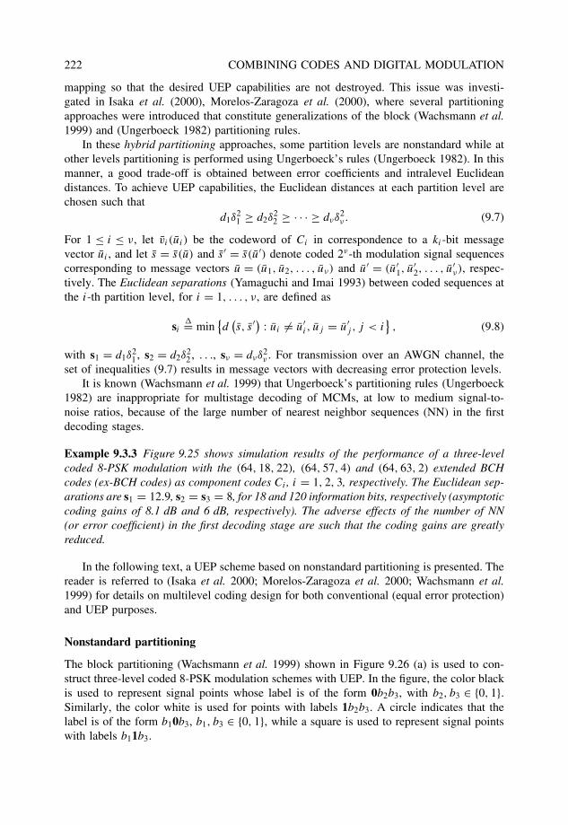
222 COMBINING CODES AND DIGITAL MODULATION
mapping so that the desired UEP capabilities are not destroyed. This issue was investi-gated in Isaka et al. (2000), Morelos-Zaragoza et al. (2000), where several partitioningapproaches were introduced that constitute generalizations of the block (Wachsmann et al.1999) and (Ungerboeck 1982) partitioning rules.
In these hybrid partitioning approaches, some partition levels are nonstandard while atother levels partitioning is performed using Ungerboeck’s rules (Ungerboeck 1982). In thismanner, a good trade-off is obtained between error coefficients and intralevel Euclideandistances. To achieve UEP capabilities, the Euclidean distances at each partition level arechosen such that
d1δ21 ≥ d2δ
22 ≥ · · · ≥ dνδ
2ν . (9.7)
For 1 ≤ i ≤ ν, let vi (ui) be the codeword of Ci in correspondence to a ki-bit messagevector ui , and let s = s(u) and s ′ = s(u′) denote coded 2ν-th modulation signal sequencescorresponding to message vectors u = (u1, u2, . . . , uν) and u′ = (u′
1, u′2, . . . , u′
ν), respec-tively. The Euclidean separations (Yamaguchi and Imai 1993) between coded sequences atthe i-th partition level, for i = 1, . . . , ν, are defined as
si�= min
{d
(s, s ′) : ui �= u′
i , uj = u′j , j < i
}, (9.8)
with s1 = d1δ21 , s2 = d2δ
22 , . . ., sν = dνδ
2ν . For transmission over an AWGN channel, the
set of inequalities (9.7) results in message vectors with decreasing error protection levels.It is known (Wachsmann et al. 1999) that Ungerboeck’s partitioning rules (Ungerboeck
1982) are inappropriate for multistage decoding of MCMs, at low to medium signal-to-noise ratios, because of the large number of nearest neighbor sequences (NN) in the firstdecoding stages.
Example 9.3.3 Figure 9.25 shows simulation results of the performance of a three-levelcoded 8-PSK modulation with the (64, 18, 22), (64, 57, 4) and (64, 63, 2) extended BCHcodes (ex-BCH codes) as component codes Ci , i = 1, 2, 3, respectively. The Euclidean sep-arations are s1 = 12.9, s2 = s3 = 8, for 18 and 120 information bits, respectively (asymptoticcoding gains of 8.1 dB and 6 dB, respectively). The adverse effects of the number of NN(or error coefficient) in the first decoding stage are such that the coding gains are greatlyreduced.
In the following text, a UEP scheme based on nonstandard partitioning is presented. Thereader is referred to (Isaka et al. 2000; Morelos-Zaragoza et al. 2000; Wachsmann et al.1999) for details on multilevel coding design for both conventional (equal error protection)and UEP purposes.
Nonstandard partitioning
The block partitioning (Wachsmann et al. 1999) shown in Figure 9.26 (a) is used to con-struct three-level coded 8-PSK modulation schemes with UEP. In the figure, the color blackis used to represent signal points whose label is of the form 0b2b3, with b2, b3 ∈ {0, 1}.Similarly, the color white is used for points with labels 1b2b3. A circle indicates that thelabel is of the form b10b3, b1, b3 ∈ {0, 1}, while a square is used to represent signal pointswith labels b11b3.
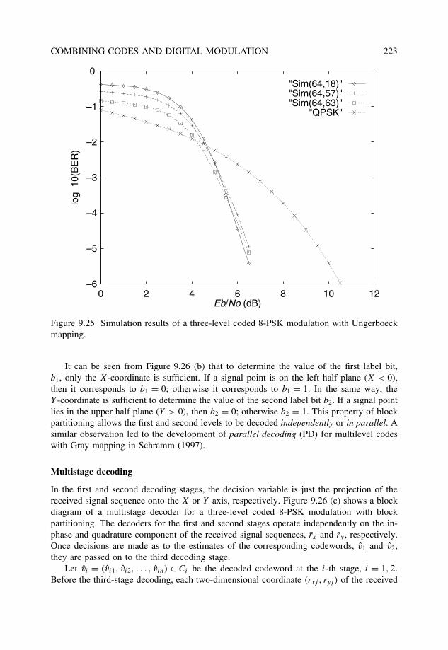
COMBINING CODES AND DIGITAL MODULATION 223
–6
–5
–4
–3
–2
–1
0
0 2 4 6 8 10 12
log_
10(B
ER
)
Eb/No (dB)
"Sim(64,18)""Sim(64,57)""Sim(64,63)"
"QPSK"
Figure 9.25 Simulation results of a three-level coded 8-PSK modulation with Ungerboeckmapping.
It can be seen from Figure 9.26 (b) that to determine the value of the first label bit,b1, only the X-coordinate is sufficient. If a signal point is on the left half plane (X < 0),then it corresponds to b1 = 0; otherwise it corresponds to b1 = 1. In the same way, theY -coordinate is sufficient to determine the value of the second label bit b2. If a signal pointlies in the upper half plane (Y > 0), then b2 = 0; otherwise b2 = 1. This property of blockpartitioning allows the first and second levels to be decoded independently or in parallel. Asimilar observation led to the development of parallel decoding (PD) for multilevel codeswith Gray mapping in Schramm (1997).
Multistage decoding
In the first and second decoding stages, the decision variable is just the projection of thereceived signal sequence onto the X or Y axis, respectively. Figure 9.26 (c) shows a blockdiagram of a multistage decoder for a three-level coded 8-PSK modulation with blockpartitioning. The decoders for the first and second stages operate independently on the in-phase and quadrature component of the received signal sequences, rx and ry , respectively.Once decisions are made as to the estimates of the corresponding codewords, v1 and v2,they are passed on to the third decoding stage.
Let vi = (vi1, vi2, . . . , vin) ∈ Ci be the decoded codeword at the i-th stage, i = 1, 2.Before the third-stage decoding, each two-dimensional coordinate (rxj , ryj ) of the received
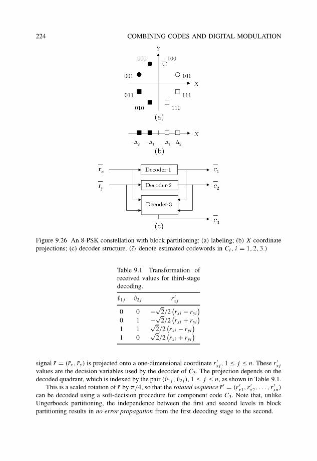
224 COMBINING CODES AND DIGITAL MODULATION
Figure 9.26 An 8-PSK constellation with block partitioning: (a) labeling; (b) X coordinateprojections; (c) decoder structure. (ci denote estimated codewords in Ci , i = 1, 2, 3.)
Table 9.1 Transformation ofreceived values for third-stagedecoding.
v1j v2j r ′xj
0 0 −√2/2
(rxi − ryi
)0 1 −√
2/2(rxi + ryi
)1 1
√2/2
(rxi − ryi
)1 0
√2/2
(rxi + ryi
)
signal r = (rx, ry) is projected onto a one-dimensional coordinate r ′xj , 1 ≤ j ≤ n. These r ′
xj
values are the decision variables used by the decoder of C3. The projection depends on thedecoded quadrant, which is indexed by the pair (v1j , v2j ), 1 ≤ j ≤ n, as shown in Table 9.1.
This is a scaled rotation of r by π/4, so that the rotated sequence r ′ = (r ′x1, r ′
x2, . . . , r ′xn)
can be decoded using a soft-decision procedure for component code C3. Note that, unlikeUngerboeck partitioning, the independence between the first and second levels in blockpartitioning results in no error propagation from the first decoding stage to the second.
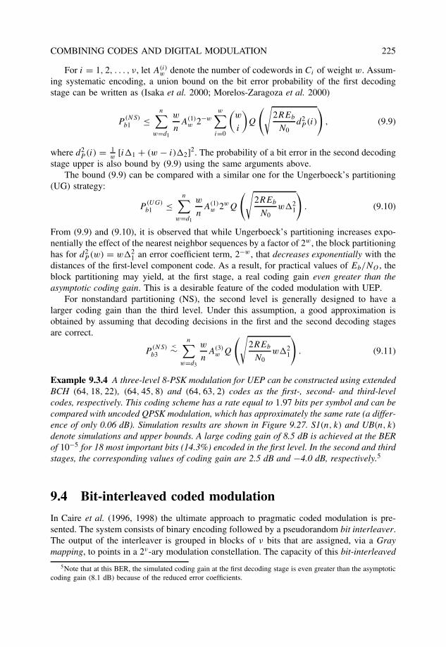
COMBINING CODES AND DIGITAL MODULATION 225
For i = 1, 2, . . . , ν, let A(i)w denote the number of codewords in Ci of weight w. Assum-
ing systematic encoding, a union bound on the bit error probability of the first decodingstage can be written as (Isaka et al. 2000; Morelos-Zaragoza et al. 2000)
P(NS)b1 ≤
n∑w=d1
w
nA(1)
w 2−w
w∑i=0
(w
i
)Q
(√2REb
N0d2
P (i)
), (9.9)
where d2P (i) = 1
w[i�1 + (w − i)�2]2. The probability of a bit error in the second decoding
stage upper is also bound by (9.9) using the same arguments above.The bound (9.9) can be compared with a similar one for the Ungerboeck’s partitioning
(UG) strategy:
P(UG)b1 ≤
n∑w=d1
w
nA(1)
w 2wQ
(√2REb
N0w�2
1
). (9.10)
From (9.9) and (9.10), it is observed that while Ungerboeck’s partitioning increases expo-nentially the effect of the nearest neighbor sequences by a factor of 2w , the block partitioninghas for d2
P (w) = w�21 an error coefficient term, 2−w , that decreases exponentially with the
distances of the first-level component code. As a result, for practical values of Eb/NO , theblock partitioning may yield, at the first stage, a real coding gain even greater than theasymptotic coding gain. This is a desirable feature of the coded modulation with UEP.
For nonstandard partitioning (NS), the second level is generally designed to have alarger coding gain than the third level. Under this assumption, a good approximation isobtained by assuming that decoding decisions in the first and the second decoding stagesare correct.
P(NS)b3
<∼n∑
w=d3
w
nA(3)
w Q
(√2REb
N0w�2
1
). (9.11)
Example 9.3.4 A three-level 8-PSK modulation for UEP can be constructed using extendedBCH (64, 18, 22), (64, 45, 8) and (64, 63, 2) codes as the first-, second- and third-levelcodes, respectively. This coding scheme has a rate equal to 1.97 bits per symbol and can becompared with uncoded QPSK modulation, which has approximately the same rate (a differ-ence of only 0.06 dB). Simulation results are shown in Figure 9.27. S1(n, k) and UB(n, k)
denote simulations and upper bounds. A large coding gain of 8.5 dB is achieved at the BERof 10−5 for 18 most important bits (14.3%) encoded in the first level. In the second and thirdstages, the corresponding values of coding gain are 2.5 dB and −4.0 dB, respectively.5
9.4 Bit-interleaved coded modulation
In Caire et al. (1996, 1998) the ultimate approach to pragmatic coded modulation is pre-sented. The system consists of binary encoding followed by a pseudorandom bit interleaver.The output of the interleaver is grouped in blocks of ν bits that are assigned, via a Graymapping, to points in a 2ν-ary modulation constellation. The capacity of this bit-interleaved
5Note that at this BER, the simulated coding gain at the first decoding stage is even greater than the asymptoticcoding gain (8.1 dB) because of the reduced error coefficients.
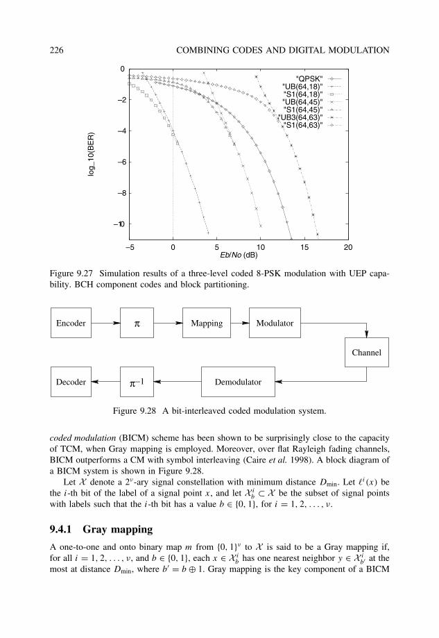
226 COMBINING CODES AND DIGITAL MODULATION
–10
–8
–6
–4
–2
0
–5 0 5 10 15 20
log_
10(B
ER
)
Eb/No (dB)
"QPSK""UB(64,18)""S1(64,18)""UB(64,45)""S1(64,45)"
"UB3(64,63)""S1(64,63)"
Figure 9.27 Simulation results of a three-level coded 8-PSK modulation with UEP capa-bility. BCH component codes and block partitioning.
Encoder
Decoder
π
π−1
Mapping Modulator
Demodulator
Channel
Figure 9.28 A bit-interleaved coded modulation system.
coded modulation (BICM) scheme has been shown to be surprisingly close to the capacityof TCM, when Gray mapping is employed. Moreover, over flat Rayleigh fading channels,BICM outperforms a CM with symbol interleaving (Caire et al. 1998). A block diagram ofa BICM system is shown in Figure 9.28.
Let X denote a 2ν-ary signal constellation with minimum distance Dmin. Let i(x) bethe i-th bit of the label of a signal point x, and let X i
b ⊂ X be the subset of signal pointswith labels such that the i-th bit has a value b ∈ {0, 1}, for i = 1, 2, . . . , ν.
9.4.1 Gray mapping
A one-to-one and onto binary map m from {0, 1}ν to X is said to be a Gray mapping if,for all i = 1, 2, . . . , ν, and b ∈ {0, 1}, each x ∈ X i
b has one nearest neighbor y ∈ X ib′ at the
most at distance Dmin, where b′ = b ⊕ 1. Gray mapping is the key component of a BICM
COMBINING CODES AND DIGITAL MODULATION 227
system. Its main function is – ideally – to produce an equivalent channel that has ν parallel,independent and memoryless, binary channels. Each channel corresponds to a position inthe label of a signal x ∈ X . For each codeword at the output of the binary encoder, theinterleaver assigns at random a position in the label of the signals to transmit the coded bits.
9.4.2 Metric generation: De-mapping
Before the description of how metrics for an MLD decoder are generated, some notation isneeded. Let r denote the channel output after transmission of x. Assuming uniform inputdistribution, the conditional probability of r given i(x) = b is
p(r|i(x) = b) =∑x∈X
p(r|x)p(x|i(x) = b) = 2−(ν−1)∑x∈X i
b
p(r|x). (9.12)
Let i denote the position of the coded bit vj in the label of xπ(j). At each time j , let vj bea code symbol and xπ(j) be the interleaved signal point, received as rπ(j) after transmissionover a noisy channel.
The receiver then produces bit metrics
λi(rπ(j), b) = log
∑
x∈X ib
p(rπ(j)|x)
, (9.13)
for b = 0, 1 and i = 1, 2, . . . , ν.An MLD algorithm, such as the Viterbi algorithm, uses the above metrics and makes
decisions on the basis of the rule
vi = arg maxv∈C
∑j
λi(rπ(j), vj ). (9.14)
As before, a max-log approximation of (9.13) is possible, resulting in the approximatedbit metric,
λia(rπ(j), b) = max
x∈X ib
log p(rπ(j)|x). (9.15)
9.4.3 Interleaving
With transmission over an AWGN channel, a short interleaver will suffice. The main purposeis to break the correlation introduced by the 2ν-ary modulation signal set, which carriesν bits per signal. Therefore, an interleaver of length equal to a few times ν is enough toapproach best performance (Caire et al. 1998). Note that this interleaver has nothing to dowith the interleaver that a turbo code or a block product code would use.
9.5 Turbo trellis-coded modulation
Conceptually, there are various approaches to the combination of turbo codes, or productcodes with interleaving, and digital modulation: pragmatic coded modulation (Le Goff et al.1994), turbo TCM with symbol interleaving (Robertson and Worz 1995, 1998) and turboTCM with bit interleaving (Benedetto et al. 1996).
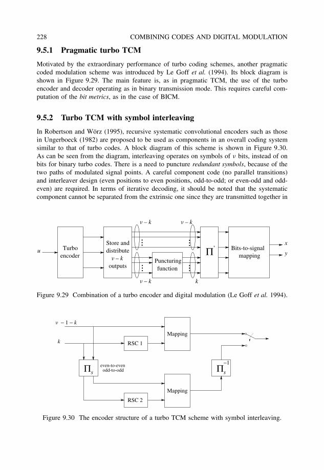
228 COMBINING CODES AND DIGITAL MODULATION
9.5.1 Pragmatic turbo TCM
Motivated by the extraordinary performance of turbo coding schemes, another pragmaticcoded modulation scheme was introduced by Le Goff et al. (1994). Its block diagram isshown in Figure 9.29. The main feature is, as in pragmatic TCM, the use of the turboencoder and decoder operating as in binary transmission mode. This requires careful com-putation of the bit metrics, as in the case of BICM.
9.5.2 Turbo TCM with symbol interleaving
In Robertson and Worz (1995), recursive systematic convolutional encoders such as thosein Ungerboeck (1982) are proposed to be used as components in an overall coding systemsimilar to that of turbo codes. A block diagram of this scheme is shown in Figure 9.30.As can be seen from the diagram, interleaving operates on symbols of ν bits, instead of onbits for binary turbo codes. There is a need to puncture redundant symbols, because of thetwo paths of modulated signal points. A careful component code (no parallel transitions)and interleaver design (even positions to even positions, odd-to-odd; or even-odd and odd-even) are required. In terms of iterative decoding, it should be noted that the systematiccomponent cannot be separated from the extrinsic one since they are transmitted together in
’
n – k Puncturingfunction
mappingBits-to-signal
...... ...
...
x
yuencoderTurbo
Store anddistribute
outputs
k
Π
n – k
n – k
n – k
Figure 9.29 Combination of a turbo encoder and digital modulation (Le Goff et al. 1994).
RSC 2
RSC 1
Πs
Mapping
Mapping
Πs
−1even-to-evenodd-to-odd
k
n − 1 − k
Figure 9.30 The encoder structure of a turbo TCM scheme with symbol interleaving.
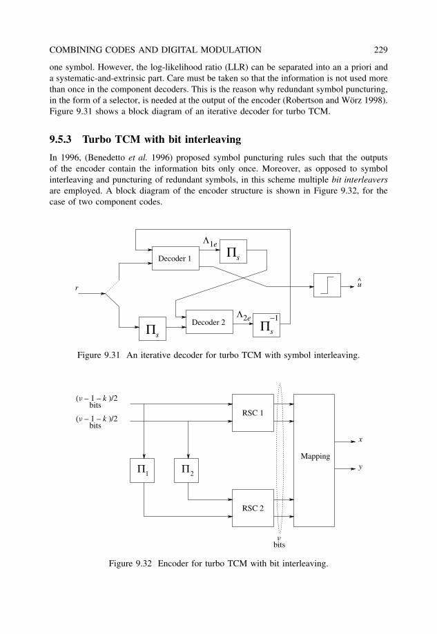
COMBINING CODES AND DIGITAL MODULATION 229
one symbol. However, the log-likelihood ratio (LLR) can be separated into an a priori anda systematic-and-extrinsic part. Care must be taken so that the information is not used morethan once in the component decoders. This is the reason why redundant symbol puncturing,in the form of a selector, is needed at the output of the encoder (Robertson and Worz 1998).Figure 9.31 shows a block diagram of an iterative decoder for turbo TCM.
9.5.3 Turbo TCM with bit interleaving
In 1996, (Benedetto et al. 1996) proposed symbol puncturing rules such that the outputsof the encoder contain the information bits only once. Moreover, as opposed to symbolinterleaving and puncturing of redundant symbols, in this scheme multiple bit interleaversare employed. A block diagram of the encoder structure is shown in Figure 9.32, for thecase of two component codes.
Πs
Πs
Πs
−1
Decoder 1
Decoder 2
u
Λ2e
Λ1e
r
Figure 9.31 An iterative decoder for turbo TCM with symbol interleaving.
Π1
(n – 1 – k )/2
(n – 1 – k )/2
Π2
RSC 1
RSC 2
Mapping
x
y
bits
bits
nbits
Figure 9.32 Encoder for turbo TCM with bit interleaving.
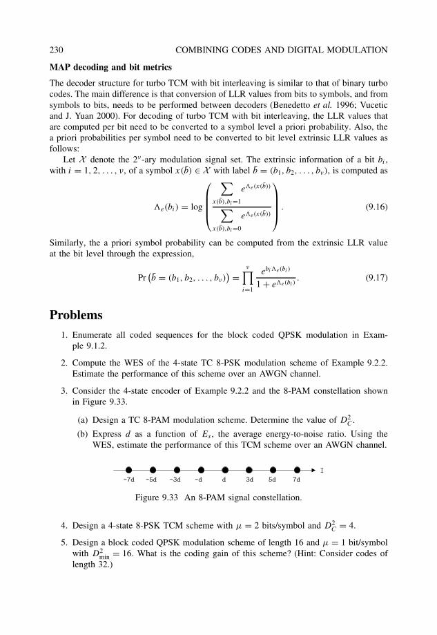
230 COMBINING CODES AND DIGITAL MODULATION
MAP decoding and bit metrics
The decoder structure for turbo TCM with bit interleaving is similar to that of binary turbocodes. The main difference is that conversion of LLR values from bits to symbols, and fromsymbols to bits, needs to be performed between decoders (Benedetto et al. 1996; Vuceticand J. Yuan 2000). For decoding of turbo TCM with bit interleaving, the LLR values thatare computed per bit need to be converted to a symbol level a priori probability. Also, thea priori probabilities per symbol need to be converted to bit level extrinsic LLR values asfollows:
Let X denote the 2ν-ary modulation signal set. The extrinsic information of a bit bi ,with i = 1, 2, . . . , ν, of a symbol x(b) ∈ X with label b = (b1, b2, . . . , bν), is computed as
e(bi) = log
∑x(b),bi=1
ee(x(b))
∑x(b),bi=0
ee(x(b))
. (9.16)
Similarly, the a priori symbol probability can be computed from the extrinsic LLR valueat the bit level through the expression,
Pr(b = (b1, b2, . . . , bν)
) =ν∏
i=1
ebie(bi )
1 + ee(bi ). (9.17)
Problems1. Enumerate all coded sequences for the block coded QPSK modulation in Exam-
ple 9.1.2.
2. Compute the WES of the 4-state TC 8-PSK modulation scheme of Example 9.2.2.Estimate the performance of this scheme over an AWGN channel.
3. Consider the 4-state encoder of Example 9.2.2 and the 8-PAM constellation shownin Figure 9.33.
(a) Design a TC 8-PAM modulation scheme. Determine the value of D2C .
(b) Express d as a function of Es , the average energy-to-noise ratio. Using theWES, estimate the performance of this TCM scheme over an AWGN channel.
I
−7d −5d −3d −d d 3d 5d 7d
Figure 9.33 An 8-PAM signal constellation.
4. Design a 4-state 8-PSK TCM scheme with µ = 2 bits/symbol and D2C = 4.
5. Design a block coded QPSK modulation scheme of length 16 and µ = 1 bit/symbolwith D2
min = 16. What is the coding gain of this scheme? (Hint: Consider codes oflength 32.)
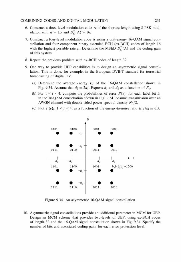
COMBINING CODES AND DIGITAL MODULATION 231
6. Construct a three-level modulation code of the shortest length using 8-PSK mod-ulation with µ ≥ 1.5 and D2
C() ≥ 16.
7. Construct a four-level modulation code using a unit-energy 16-QAM signal con-stellation and four component binary extended BCH (ex-BCH) codes of length 16with the highest possible rate µ. Determine the MSED D2
C() and the coding gainof this system.
8. Repeat the previous problem with ex-BCH codes of length 32.
9. One way to provide UEP capabilities is to design an asymmetric signal constel-lation. This is done, for example, in the European DVB-T standard for terrestrialbroadcasting of digital TV.
(a) Determine the average energy Es of the 16-QAM constellation shown inFig. 9.34. Assume that d2 = 2d1. Express d1 and d2 as a function of Es .
(b) For 1 ≤ i ≤ 4, compute the probabilities of error P {e}i for each label bit bi
in the 16-QAM constellation shown in Fig. 9.34. Assume transmission over anAWGN channel with double-sided power spectral density N0/2.
(c) Plot P {e}i , 1 ≤ i ≤ 4, as a function of the energy-to-noise ratio Es/N0 in dB.
b0b1b2b3 =1000
Q
I
00000001
00100011
01000101
01100111
11001101
11101111
1001
10101011
d2
d− 2 d− 1 d1 d2
d− 1
d− 2
d1
Figure 9.34 An asymmetric 16-QAM signal constellation.
10. Asymmetric signal constellations provide an additional parameter in MCM for UEP.Design an MCM scheme that provides two-levels of UEP, using ex-BCH codesof length 32 and the 16-QAM signal constellation shown in Fig. 9.34. Specify thenumber of bits and associated coding gain, for each error protection level.
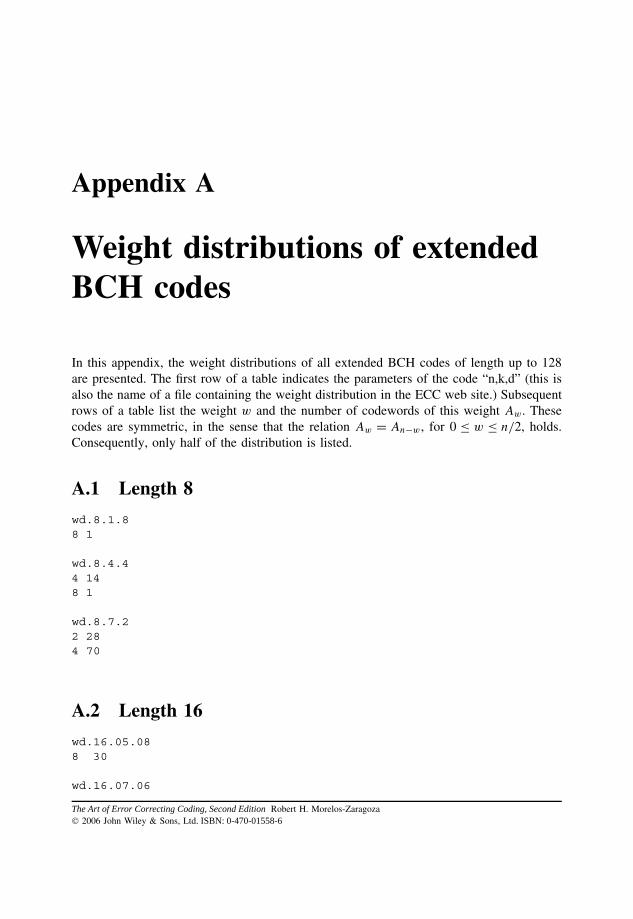
Appendix A
Weight distributions of extendedBCH codes
In this appendix, the weight distributions of all extended BCH codes of length up to 128are presented. The first row of a table indicates the parameters of the code “n,k,d” (this isalso the name of a file containing the weight distribution in the ECC web site.) Subsequentrows of a table list the weight w and the number of codewords of this weight Aw. Thesecodes are symmetric, in the sense that the relation Aw = An−w, for 0 ≤ w ≤ n/2, holds.Consequently, only half of the distribution is listed.
A.1 Length 8
wd.8.1.88 1
wd.8.4.44 148 1
wd.8.7.22 284 70
A.2 Length 16
wd.16.05.088 30
wd.16.07.06
The Art of Error Correcting Coding, Second Edition Robert H. Morelos-Zaragoza 2006 John Wiley & Sons, Ltd. ISBN: 0-470-01558-6
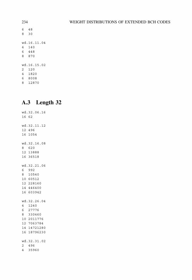
234 WEIGHT DISTRIBUTIONS OF EXTENDED BCH CODES
6 488 30
wd.16.11.044 1406 4488 870
wd.16.15.022 1204 18206 80088 12870
A.3 Length 32
wd.32.06.1616 62
wd.32.11.1212 49616 1054
wd.32.16.088 62012 1388816 36518
wd.32.21.066 9928 1054010 6051212 22816014 44640016 603942
wd.32.26.044 12406 277768 33046010 201177612 706378414 1472128016 18796230
wd.32.31.022 4964 35960

WEIGHT DISTRIBUTIONS OF EXTENDED BCH CODES 235
6 9061928 1051830010 6451224012 22579284014 47143560016 601080390
A.4 Length 64
wd.64.07.3232 126
wd.64.10.2828 44832 126
wd.64.16.2424 504028 1254432 30366
wd.64.18.2222 422424 504026 2419228 1254430 6988832 30366
wd.64.24.1616 260418 1075222 21657624 29164826 164505628 88883230 441907232 1828134
wd.64.30.1414 806416 3082818 63168020 112896022 1402214424 1462944026 10505779228 65046016
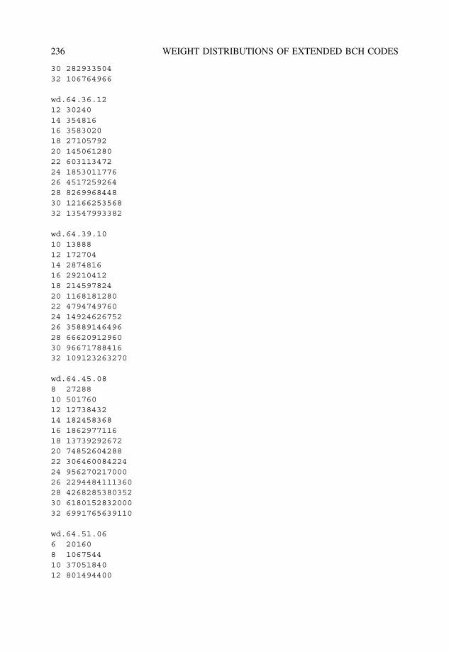
236 WEIGHT DISTRIBUTIONS OF EXTENDED BCH CODES
30 28293350432 106764966
wd.64.36.1212 3024014 35481616 358302018 2710579220 14506128022 60311347224 185301177626 451725926428 826996844830 1216625356832 13547993382
wd.64.39.1010 1388812 17270414 287481616 2921041218 21459782420 116818128022 479474976024 1492462675226 3588914649628 6662091296030 9667178841632 109123263270
wd.64.45.088 2728810 50176012 1273843214 18245836816 186297711618 1373929267220 7485260428822 30646008422424 95627021700026 229448411136028 426828538035230 618015283200032 6991765639110
wd.64.51.066 201608 106754410 3705184012 801494400
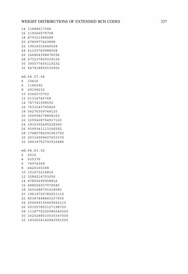
WEIGHT DISTRIBUTIONS OF EXTENDED BCH CODES 237
14 1168461734416 11926657570818 87932194828820 478997742988822 1961603244652824 6119376998800826 14686439847609628 27313780933913630 39557740511923232 447418802536902
wd.64.57.044 104166 11665928 6919423210 236657075212 5131674676814 74774199859216 763324374582018 5627635974912020 30655827885816022 125542875491712024 391639249522836026 939934111316659228 1748078629196379230 2531699960765337632 28634752793916486
wd.64.63.022 20164 6353766 749743688 442616536810 15147321481612 328421470305614 4785569995881616 48852693707958018 360168879101808020 1961972578265111622 8034744844323793624 25064910546966611026 60155785312719872028 111877029298524020030 162028801053034700032 1832624140942591500
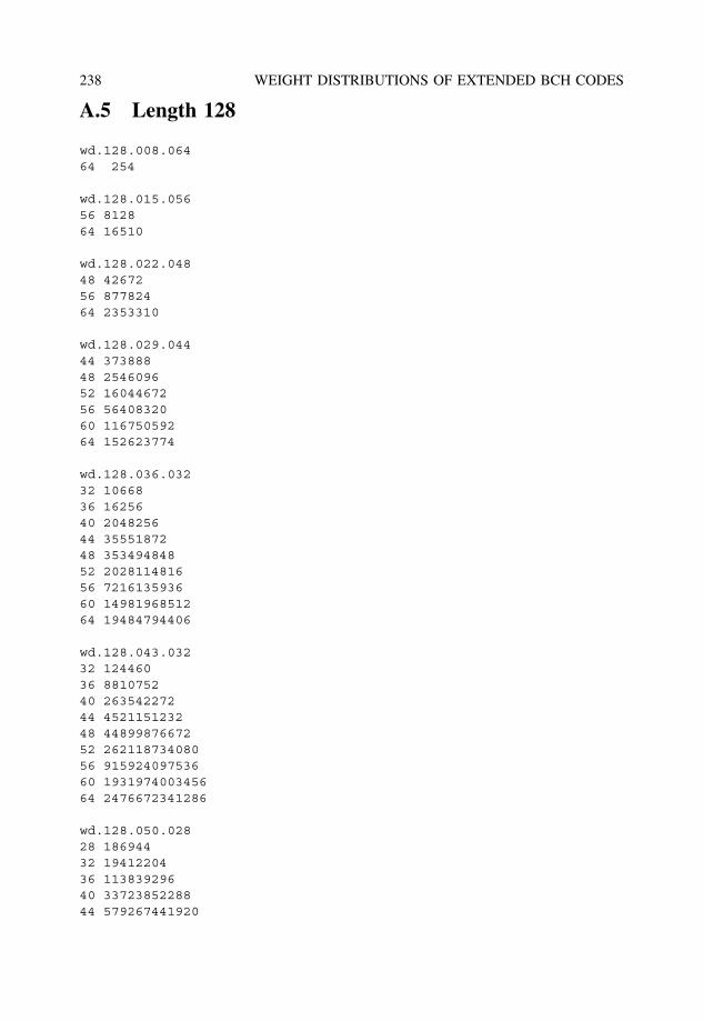
238 WEIGHT DISTRIBUTIONS OF EXTENDED BCH CODES
A.5 Length 128
wd.128.008.06464 254
wd.128.015.05656 812864 16510
wd.128.022.04848 4267256 87782464 2353310
wd.128.029.04444 37388848 254609652 1604467256 5640832060 11675059264 152623774
wd.128.036.03232 1066836 1625640 204825644 3555187248 35349484852 202811481656 721613593660 1498196851264 19484794406
wd.128.043.03232 12446036 881075240 26354227244 452115123248 4489987667252 26211873408056 91592409753660 193197400345664 2476672341286
wd.128.050.02828 18694432 1941220436 11383929640 3372385228844 579267441920
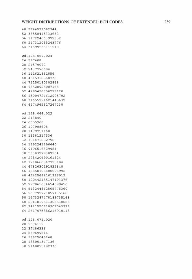
WEIGHT DISTRIBUTIONS OF EXTENDED BCH CODES 239
48 574452108294452 3355841533363256 11722466397235260 24731208524377664 31699236111910
wd.128.057.02424 59740828 2457907232 243777668436 14162188185640 431531856873644 7415018030284848 7352892500716852 429549635622912056 1500472461290579260 3165599162144563264 4574965317267238
wd.128.064.02222 24384024 685596826 10798860828 147975116830 1658121753632 16147188279634 129224129664036 910651632998438 5338327930790440 27842069016182442 121866684772518444 478263019182284846 1585870560059699248 4742568416132691250 12044218514749337652 27706163465409945654 54324486250577536056 96779972185713516858 147328747818973516860 204181951130853068862 242155063090704332864 2617075886216910118
wd.128.071.02020 267411222 3748633624 83969961626 1382504524828 18800134713630 2140095182336
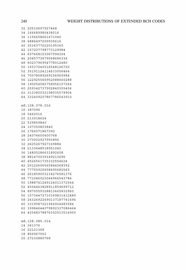
240 WEIGHT DISTRIBUTIONS OF EXTENDED BCH CODES
32 2051069792746834 16668998043801636 115665866147104038 688649720993561640 3536377622019536042 15720779877312998444 60746816306799430446 204577367906868633648 602379695477801248050 1553704051654812672052 3519112411463300646454 7007858926915696998456 12292556695208866028858 19005408275895610726460 25934273790284035545662 31238003219803557990464 332409207867786543910
wd.128.078.01616 38709618 546201620 21301862422 53985984024 10735080384026 176607186739228 2407465040076830 27393292799385632 262526756716988434 213364851895104036 1480528663189260838 88147003914921369640 452656173533255462442 2012260656584406835244 7775592565849568256046 26185900313427658137648 77104602304496654378450 198874124912401137254452 450446382891185969971254 897005932881366583296056 1573447271016983141248058 2432692269013718774169660 331958722194492448358462 3998464407989233708646464 42548378876302513514950
wd.128.085.01414 34137616 2212136818 85696755220 27230880768
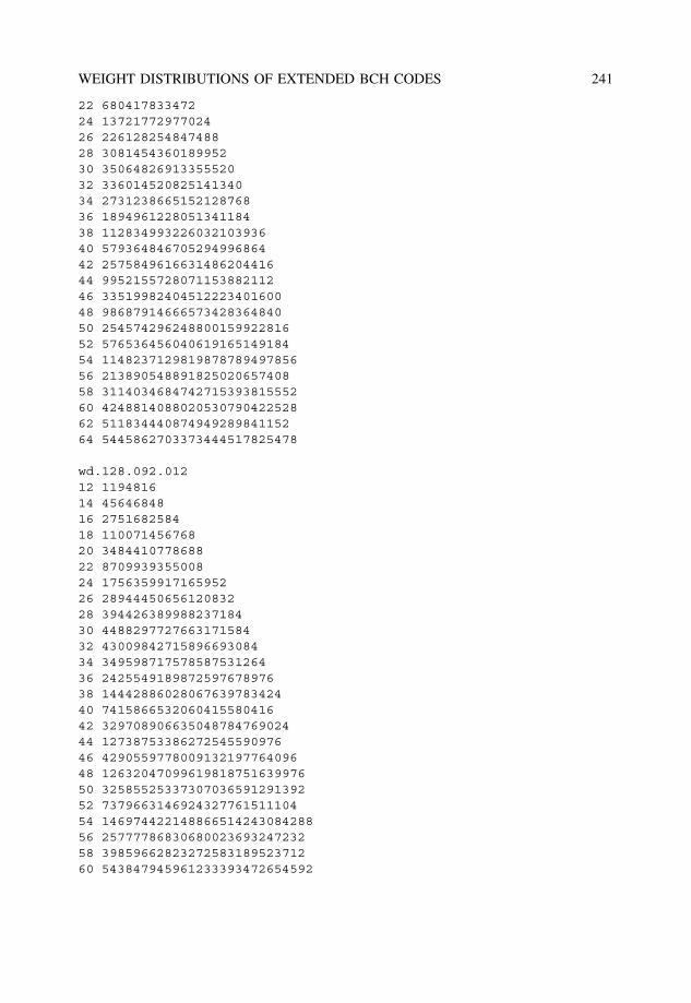
WEIGHT DISTRIBUTIONS OF EXTENDED BCH CODES 241
22 68041783347224 1372177297702426 22612825484748828 308145436018995230 3506482691335552032 33601452082514134034 273123866515212876836 189496122805134118438 11283499322603210393640 57936484670529499686442 257584961663148620441644 995215572807115388211246 3351998240451222340160048 9868791466657342836484050 25457429624880015992281652 57653645604061916514918454 114823712981987878949785656 21389054889182502065740858 311403468474271539381555260 424881408802053079042252862 51183444087494928984115264 5445862703373444517825478
wd.128.092.01212 119481614 4564684816 275168258418 11007145676820 348441077868822 870993935500824 175635991716595226 2894445065612083228 39442638998823718430 448829772766317158432 4300984271589669308434 34959871757858753126436 242554918987259767897638 1444288602806763978342440 741586653206041558041642 32970890663504878476902444 1273875338627254559097646 429055977800913219776409648 1263204709961981875163997650 3258552533730703659129139252 737966314692432776151110454 14697442214886651424308428856 2577778683068002369324723258 3985966282327258318952371260 543847945961233393472654592
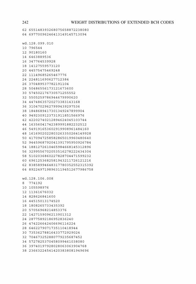
242 WEIGHT DISTRIBUTIONS OF EXTENDED BCH CODES
62 65514839326807565887223808064 69770096246413149145713094
wd.128.099.01010 79654412 9018016014 646388953616 34776453992818 1412755957312020 4457547546924822 1114968526546777624 22481169062771238426 37048953778219110428 5048655617312167360030 57450217673057125555232 550525978694467999062034 4474863572027338314316836 3104702962799943929753638 184868941730134924789990440 949230912373191185156697642 4220274021289462404510374444 1635604174238999188223251246 54919165360291990896148416048 161690202280326335026414992850 417094725858286501996048064052 944596879204139179595092678454 188127261046598466814531289656 329955670205351627822243430458 510203686022782870447159923260 696125368258194321172612121662 8385899464831778035255231539264 89224971989631194512677986758
wd.128.106.0088 77419210 10559897612 1136167603214 82862684160016 4451501317452018 180826573343539220 5705696821485337622 142715909621390131224 2877589218695283624026 47422664240669611622428 646227907173511041894430 7353627881643377292902432 70467325288077923568745234 572782537045809946103808036 3974019792802806306390476838 236632245414203838081949696
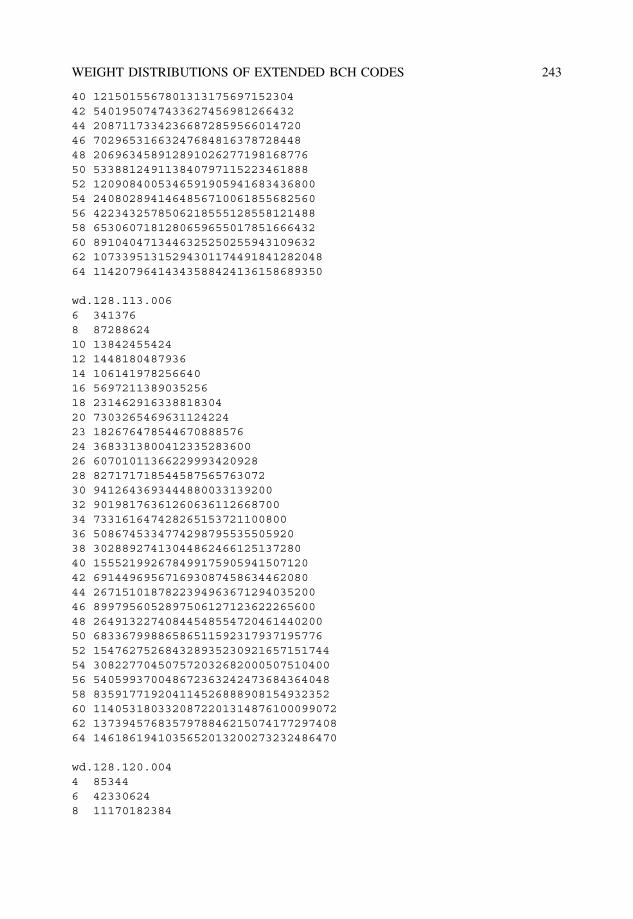
WEIGHT DISTRIBUTIONS OF EXTENDED BCH CODES 243
40 121501556780131317569715230442 540195074743362745698126643244 2087117334236687285956601472046 7029653166324768481637872844848 20696345891289102627719816877650 53388124911384079711522346188852 120908400534659190594168343680054 240802894146485671006185568256056 422343257850621855512855812148858 653060718128065965501785166643260 891040471344632525025594310963262 1073395131529430117449184128204864 11420796414343588424136158689350
wd.128.113.0066 3413768 8728862410 1384245542412 144818048793614 10614197825664016 569721138903525618 23146291633881830420 730326546963112422423 18267647854467088857624 368331380041233528360026 6070101136622999342092828 82717171854458756576307230 941264369344488003313920032 9019817636126063611266870034 73316164742826515372110080036 508674533477429879553550592038 3028892741304486246612513728040 15552199267849917590594150712042 69144969567169308745863446208044 267151018782239496367129403520046 899795605289750612712362226560048 2649132274084454855472046144020050 6833679988658651159231793719577652 15476275268432893523092165715174454 30822770450757203268200050751040056 54059937004867236324247368436404858 83591771920411452688890815493235260 114053180332087220131487610009907262 137394576835797884621507417729740864 1461861941035652013200273232486470
wd.128.120.0044 853446 423306248 11170182384
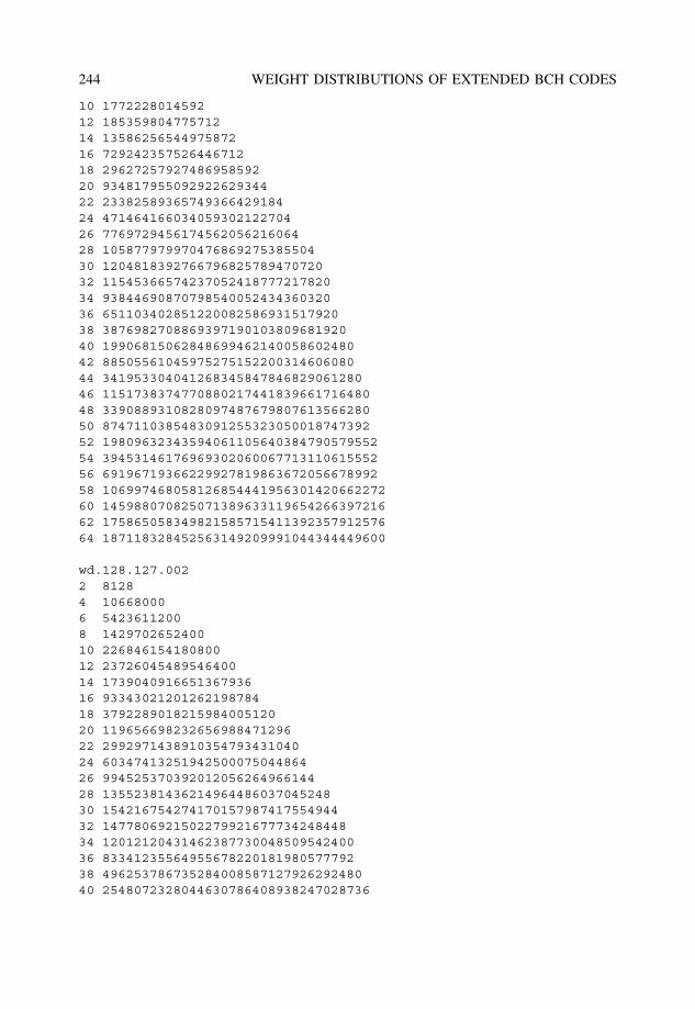
244 WEIGHT DISTRIBUTIONS OF EXTENDED BCH CODES
10 177222801459212 18535980477571214 1358625654497587216 72924235752644671218 2962725792748695859220 93481795509292262934422 2338258936574936642918424 47146416603405930212270426 776972945617456205621606428 10587797997047686927538550430 120481839276679682578947072032 1154536657423705241877721782034 9384469087079854005243436032036 65110340285122008258693151792038 387698270886939719010380968192040 1990681506284869946214005860248042 8850556104597527515220031460608044 34195330404126834584784682906128046 115173837477088021744183966171648048 339088931082809748767980761356628050 874711038548309125532305001874739252 1980963234359406110564038479057955254 3945314617696930206006771311061555256 6919671936622992781986367205667899258 10699746805812685444195630142066227260 14598807082507138963311965426639721662 17586505834982158571541139235791257664 187118328452563149209991044344449600
wd.128.127.0022 81284 106680006 54236112008 142970265240010 22684615418080012 2372604548954640014 173904091665136793616 9334302120126219878418 379228901821598400512020 11965669823265698847129622 299297143891035479343104024 6034741325194250007504486426 99452537039201205626496614428 1355238143621496448603704524830 15421675427417015798741755494432 147780692150227992167773424844834 1201212043146238773004850954240036 8334123556495567822018198057779238 49625378673528400858712792629248040 2548072328044630786408938247028736
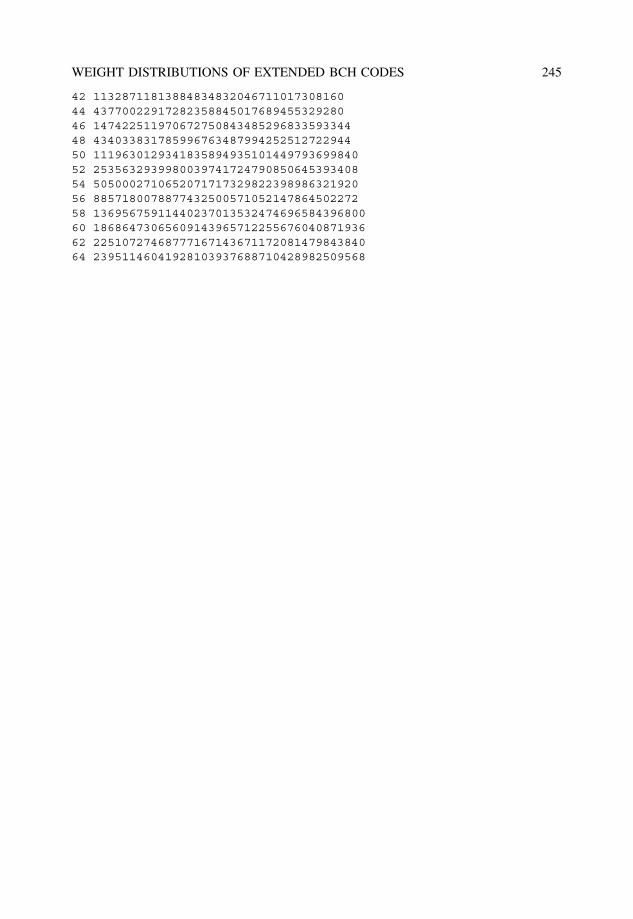
WEIGHT DISTRIBUTIONS OF EXTENDED BCH CODES 245
42 1132871181388483483204671101730816044 4377002291728235884501768945532928046 14742251197067275084348529683359334448 43403383178599676348799425251272294450 111963012934183589493510144979369984052 253563293998003974172479085064539340854 505000271065207171732982239898632192056 885718007887743250057105214786450227258 1369567591144023701353247469658439680060 1868647306560914396571225567604087193662 2251072746877716714367117208147984384064 23951146041928103937688710428982509568
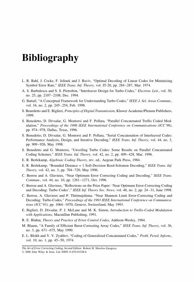
Bibliography
L. R. Bahl, J. Cocke, F. Jelinek and J. Raviv, “Optimal Decoding of Linear Codes for MinimizingSymbol Error Rate,” IEEE Trans. Inf. Theory, vol. IT-20, pp. 284–287, Mar. 1974.
A. S. Barbulescu and S. S. Pietrobon, “Interleaver Design for Turbo Codes,” Electron. Lett., vol. 30,no. 25, pp. 2107–2108, Dec. 1994.
G. Battail, “A Conceptual Framework for Understanding Turbo Codes,” IEEE J. Sel. Areas Commun.,vol. 16, no. 2, pp. 245–254, Feb. 1998.
S. Benedetto and E. Biglieri, Principles of Digital Transmission, Kluwer Academic/Plenum Publishers,1999.
S. Benedetto, D. Divsalar, G. Montorsi and F. Pollara, “Parallel Concatenated Trellis Coded Mod-ulation,” Proceedings of the 1996 IEEE International Conference on Communications (ICC’96),pp. 974–978, Dallas, Texas, 1996.
S. Benedetto, D. Divsalar, G. Montorsi and F. Pollara, “Serial Concatenation of Interleaved Codes:Performance Analysis, Design, and Iterative Decoding,” IEEE Trans. Inf. Theory, vol. 44, no. 3,pp. 909–926, May 1998.
S. Benedetto and G. Montorsi, “Unveiling Turbo Codes: Some Results on Parallel ConcatenatedCoding Schemes,” IEEE Trans. Inf. Theory, vol. 42, no. 2, pp. 409–428, Mar. 1996.
E. R. Berlekamp, Algebraic Coding Theory, rev. ed., Aegean Park Press, 1984.
E. R. Berlekamp, “Bounded Distance + 1 Soft-Decision Reed-Solomon Decoding,” IEEE Trans. Inf.Theory, vol. 42, no. 3, pp. 704–720, May 1996.
C. Berrou and A. Glavieux, “Near Optimum Error Correcting Coding and Decoding,” IEEE Trans.Commun., vol. 44, no. 10, pp. 1261–1271, Oct. 1996.
C. Berrou and A. Glavieux, “Reflections on the Prize Paper: ‘Near Optimum Error-Correcting Codingand Decoding: Turbo Codes’,” IEEE Inf. Theory Soc. News, vol. 48, no. 2, pp. 24–31, June 1998.
C. Berrou, A. Glavieux and P. Thitimajshima, “Near Shannon Limit Error-Correcting Coding andDecoding: Turbo-Codes,” Proceedings of the 1993 IEEE International Conference on Communica-tions (ICC’93), pp. 1064–1070, Geneve, Switzerland, May 1993.
E. Biglieri, D. Divsalar, P. J. McLane and M. K. Simon, Introduction to Trellis-Coded Modulationwith Applications, Macmillan Publishing, 1991.
R. E. Blahut, Theory and Practice of Error Control Codes, Addison-Wesley, 1984.
M. Blaum, “A Family of Efficient Burst-Correcting Array Codes,” IEEE Trans. Inf. Theory, vol. 36,no. 3, pp. 671–675, May 1990.
E. L. Blokh and V. V. Zyablov, “Coding of Generalized Concatenated Codes,” Probl. Pered. Inform.,vol. 10, no. 1, pp. 45–50, 1974.
The Art of Error Correcting Coding, Second Edition Robert H. Morelos-Zaragoza 2006 John Wiley & Sons, Ltd. ISBN: 0-470-01558-6
248 BIBLIOGRAPHY
M. Boo, F. Arguello, J. D. Bruguera, R. Doallo and E. L. Zapata, “High-Performance VLSI Archi-tecture for the Viterbi Algorithm,” IEEE Trans. Commun., vol. 45, no. 2, pp. 168–176, Feb.1997.
M. Bossert, Channel Coding for Telecommunications, John Wiley & Sons, 1999.
M. Breiling and J. B. Huber, “Combinatorial Analysis of the Minimum Distance of Turbo Codes,”IEEE Trans. Inf. Theory, vol. 47, no. 7, pp. 2737–2750, Nov. 2001.
A. E. Brouwer and T. Verhoeff, “An Updated Table of Minimum-Distance Bounds for Binary LinearCodes,” IEEE Trans. Inf. Theory, vol. 39, no. 2, pp. 662–677, Mar. 1993.
H. O. Burton and E. J. Weldon, Jr., “Cyclic Product Codes,” IEEE Trans. Inf. Theory, vol. IT-11, no.3, pp. 433–439, July 1965.
J. B. Cain, G. C Clark and J. M. Geist, “Punctured Convolutional Codes of Rate (n − 1)/n andSimplified Maximum Likelihood Decoding,” IEEE Trans. Inf. Theory, vol. IT-25, pp. 97–100,Jan. 1979.
G. Caire, G. Taricco and E. Biglieri, “Capacity of Bit-Interleaved Channels,” Electron. Lett., vol. 32,pp. 1060–1061, June 1996.
G. Caire, G. Taricco and E. Biglieri, “Bit-Interleaver Coded Modulation,” IEEE Trans. Inf. Theory,vol. 44, no. 3, pp. 927–946, May 1998.
F. Carden, M. D. Ross, B. T. Kopp and W. P. Osborn, “Fast TCM Decoding: Phase Quantizationand Integer Weighting,” IEEE Trans. Commun., vol. 42, no. 4, pp. 808–812, Apr. 1994.
C.-C. Chao and Y.-L. Yao, “Hidden Markov Models for the Burst Error Statistics of Viterbi Decoding,”IEEE Trans. Commun., vol. 44, no. 12, pp. 1620–1622, Dec. 1996.
D. Chase, “A Class of Algorithms for Decoding Block Codes with Channel Measurement Informa-tion,” IEEE Trans. Inf. Theory, vol. IT-18, pp. 170–182, 1972.
P. Chaudhari and A. K. Khandani, “Using the Fourier Transform to Compute the Weight Distributionof a Binary Linear Block Code,” IEEE Commun. Lett., vol. 5, no. 1, pp. 22–24, Jan. 2001.
S.-Y. Chung, G. D. Forney, Jr., T. J. Richardson and R. Urbanke, “On the Design of Low-DensityParity-Check Codes within 0.0045 dB of the Shannon Limit,” IEEE Commun. Lett., vol. 5, no. 2,pp. 58–60, Feb. 2001.
G. Clark and J. Cain, Error-Correction Coding for Digital Communications, Plenum Press, 1981.
O. M. Collins, “The Subtleties and Intricacies of Building a Constraint Length 15 ConvolutionalDecoder,” IEEE Trans. Commun., vol. 40, no. 12, pp. 1810–1819, Nov. 1992.
T. M. Cover and J. A. Thomas, Elements of Information Theory, John Wiley & Sons, 1991.
Y. Desaki, T. Fujiwara and T. Kasami, “A Method for Computing the Weight Distribution of a BlockCode by Using Its Trellis Diagram,” IEICE Trans. Fundamentals, vol. E77-A, pp. 1230–1237,Aug. 1994.
Y. Desaki, T. Fujiwara and T. Kasami, “The Weight Distribution of Extended Binary Primitive BCHCodes of Length 128,” IEEE Trans. Inf. Theory, vol. 43, no. 4, pp. 1364–1371, July 1997.
U. Dettmar, G. Yan and U. K. Sorger, “Modified Generalized Concatenated Codes and Their Appli-cation to the Construction and Decoding of LUEP Codes,” IEEE Trans. Inf. Theory, vol. 41, no.5, pp. 1499–1503, Sept. 1995.
A. Dholakia, Introduction to Convolutional Codes With Applications, Kluwer, 1994.
D. Divsalar, S. Dolinar and F. Pollara, “Iterative Turbo Decoder Analysis Based on Density Evolu-tion,” IEEE J. Sel. Areas Commun., vol. 19, no. 5, pp. 891–907, May 2001.
D. Divsalar, H. Jin and R. J. McEliece, “Coding Theorems for Turbo-Like Codes,” Proceedings of the1998 Allerton Conference on Communications, Control, and Computing, pp. 210–219, Universityof Illinois, Urbana-Champaign, IL, 1998.
BIBLIOGRAPHY 249
D. Divsalar and F. Pollara, “Turbo Codes for PCS Applications,” Proceedings of the 1993 IEEEInternational Conference on Communications (ICC’93), pp. 1064–1070, Geneva, Switzerland, May1993.
D. Divsalar and F. Pollara, “Turbo Codes for Deep-Space Communications,” JPL TDA ProgressReport 42-120, NASA Jet Propulsion Laboratory, pp. 29–39, Feb. 1995.
H. El Gamal and A. R. Hammons, Jr., “Analyzing the Turbo Decoder Using the Gaussian Approxi-mation,” IEEE Trans. Inf. Theory, vol. 47, no. 2, pp. 671–686, Feb. 2001.
P. Elias, “Error-Free Coding,” IRE Trans., vol. PGIT-4, pp. 29–37, 1954.P. Elias, “Coding for Noisy Channels,” IRE Conv. Rec., vol. 3, pt. 4, pp. 37–46, 1955; Also in E. R.
Berlekamp, ed., Key Papers in the Development of Coding Theory, pp. 48–55, IEEE Press, 1974.P. Elias, “Error-Correcting Codes for List Decoding,” IEEE Trans. Inf. Theory, vol. 37, no. 1, pp.
5–12, Jan. 1991.EN 310 210, ETSI, “Digital Video Broadcasting (DVB): Framing Structure, Channel Coding and
Modulation for Digital Satellite News Gathering (DSNG) and Other Contribution Applications bySatellite,” Mar. 1997.
W. Feng and B. Vucetic, “A List Bidirectional Soft Output Decoder of Turbo Codes,” Proceedingsof the International Symposium on Turbo Codes and Related Topics, pp. 288–292, Brest, France,Sept. 3-5, 1997.
G. D. Forney, Jr., Concatenated Codes, Research Monograph 37, MIT Press, 1966a.G. D. Forney, “Generalized Minimum Distance Decoding,” IEEE Trans. Inf. Theory, vol. IT-12, pp.
125–131, April 1966b.G. D. Forney, “Convolutional Codes I: Algebraic Structure,” IEEE Trans. Inf. Theory, vol. IT-16, no.
6, pp. 720–738, Nov. 1970.G. D. Forney, Jr., “Burst Correcting Codes for the Classic Bursty Channel,” IEEE Trans. Commun.
Technol., vol. COM-19, pp. 772–281, 1971.G. D. Forney, Jr., “On Decoding BCH Codes,” IEEE Trans. Inf. Theory, vol. IT-11, pp. 393–403,
Oct. 1965; Also in E. R. Berlekamp, ed., Key Papers in the Development of Coding Theory, pp.149–155, IEEE Press, 1974.
G. D. Forney, Jr., “Coset Codes II: Binary Lattices and Related Codes,” IEEE Trans. Inf. Theory,vol. 24, no. 5, pp. 1152–1187, Sept. 1988.
G. D. Forney and G. Ungerboeck, “Modulation and Coding for Linear Gaussian Channels,” IEEETrans. Inf. Theory, Special Commemorative Issue, vol. 44, no. 6, pp. 2384–2415, Oct. 1998.
G. D. Forney, “Codes on Graphs: Normal Realizations,” IEEE Trans. Inf. Theory, vol. 47, no. 2, pp.520–548, Feb. 2001.
M. P. C. Fossorier, F. Burkert, S. Lin and J. Hagenauer, “On the Equivalence Between SOVA andMax-Log-MAP Decodings,” IEEE Commun. Lett., vol. 2, no. 5, pp. 137–139, May 1998.
M. P. C. Fossorier and S. Lin, “Soft-Decision Decoding on Linear Block Codes Based on OrderedStatistics,” IEEE Trans. Inf. Theory, vol. 41, no. 5, pp. 1379–1396, Sept. 1995.
M. P. C. Fossorier and S. Lin, “Some Decomposable Codes: The |a + x|b + x|a + b + x| Construc-tion,” IEEE Trans. Inf. Theory, vol. 43, no. 5, pp. 1663–1667, Sept. 1997a.
M. P. C. Fossorier and S. Lin, “Complementary Reliability-Based Soft-Decision Decoding of LinearBlock Codes Based on Ordered Statistics,” IEEE Trans. Inf. Theory, vol. 42, no. 5, pp. 1667–1672,Sep. 1997b.
M. P. C. Fossorier and S. Lin, “Soft-Input Soft-Output Decoding of Linear Block Codes Basedon Ordered Statistics,” Proceedings of the 1998 IEEE Global Telecommunications Conference(GLOBECOM’98), pp. 2828–2833, Sydney, Australia, Nov. 1998.
M. P. C. Fossorier and S. Lin, “Differential Trellis Decoding of Convolutional Codes,” IEEE Trans.Inf. Theory, vol. 46, no. 3, pp. 1046–1053, May 2000.
250 BIBLIOGRAPHY
M. P. C. Fossorier, S. Lin and D. J. Costello, Jr., “On the Weight Distribution of Terminated Convo-lutional Codes,” IEEE Trans. Inf. Theory, vol. 45, no. 5, pp. 1646–1648, July 1999.
M. P. C. Fossorier, S. Lin and D. Rhee, “Bit-Error Probability for Maximum-Likelihood Decodingof Linear Block Codes and Related Soft-Decision Decoding Methods,” IEEE Trans. Inf. Theory,vol. 44, no. 7, pp. 3083–3090, Nov. 1998.
M. P. C. Fossorier, M. Mihaljevic and H. Imai, “Reduced Complexity Iterative Decoding of Low-Density Parity Check Codes Based on Belief Propagation,” IEEE Trans. Commun., vol. 47, no. 5,pp. 673–680, May 1999.
B. J. Frey and F. R. Kschischang, “Early Detection and Trellis Splicing: Reduced-Complexity IterativeDecoding,” IEEE J. Sel. Areas Commun., vol. 16, no. 2, pp. 153–159, Feb. 1998.
T. Fujiwara, T. Kasami, A. Kitai and S. Lin, “On the Undetected Error Probability of ShortenedHamming Codes,” IEEE Trans. Commun., vol. COM-33, pp. 570–574, June 1985.
R. G. Gallager, “Low-Density Parity-Check Codes,” IRE Trans. Inf. Theory, vol. 8, no. 1, pp. 21–28,Jan. 1962.
R. Garello, P. Perleoni and S. Benedetto, “Computing the Free Distance of Turbo Codes and SeriallyConcatenated Codes with Interleavers: Algorithms and Applications,” IEEE J. Sel. Areas Commun.,vol. 19, no. 5, pp. 800–812, May 2001.
M. J. E. Golay, “Notes on Digital Coding” Proc. IRE, vol. 37, p. 657, June 1949; Also in E. R.Berlekamp, ed., Key Papers in the Development of Coding Theory, p. 13, IEEE Press, 1974.
J. D. Golic, “Iterative Optimum Symbol-by-Symbol Decoding and Fast Correlation Attacks,” IEEETrans. Inf. Theory, vol. 47, no. 7, pp. 3040–3049, Nov. 2001.
D. Gorenstein and N. Zierler, “A Class of Error Correcting Codes in pm Symbols,” J. SIAM, vol. 9,pp. 207–214, June 1961.
V. Guruswami and M. Sudan, “Improved Decoding of Reed-Solomon and Algebraic-GeometryCodes,” IEEE Trans. Inf. Theory, vol. 45, no. 6, pp. 1757–1767, Sep. 1999.
J. Hagenauer, “Rate-Compatible Punctured Convolutional Codes (RCPC Codes) and their Applica-tions,” IEEE Trans. Commun., vol. 36, no. 4, pp. 389–400, April 1988.
J. Hagenauer and P. Hoeher, “A Viterbi Algorithm with Soft-Decision Outputs and Its Applica-tions,” Proceedings of the 1989 IEEE Global Telecommunications Conference (GLOBECOM’89),pp. 47.1.1–47.1.7, Dallas, Texas, 1989.
J. Hagenauer, E. Offer and L. Papke, “Iterative Decoding of Binary Block and Convolutional Codes,”IEEE Trans. Inf. Theory, vol. 42, no. 2, pp. 429–445, Mar. 1996.
E. K. Hall and S. G. Wilson, “Stream-Oriented Turbo Codes,” IEEE Trans. Inf. Theory, vol. 47, no.5, pp. 1813–1831, July 2001.
R. W. Hamming, “Error Detecting and Error Correcting Codes,” Bell Syst. Tech. J., vol. 29, pp.147–160, 1950; Also in E. R. Berlekamp, ed., Key Papers in the Development of Coding Theory,pp. 9–12, IEEE Press, 1974.
S. Haykin, Digital Communications, 4th ed., John Wiley and Sons, 2001.C. Heegard and S. B. Wicker, Turbo Coding, Kluwer Academic Press, 1999.A. P. Hekstra, “An Alternative to Metric Rescaling in Viterbi Decoder,” IEEE Trans. Commun., vol.
37, no. 11, pp. 1220–1222, Nov. 1989.I. N. Herstein, Topics in Algebra, 2nd ed., John Wiley and Sons, 1975.J. Hokfelt, O. Edfors and T. Maseng, “A Turbo Code Interleaver Design Criterion Based on the
Performance of Iterative Decoding,” IEEE Commun. Lett., vol. 5, no. 2, pp. 52–54, Feb. 2001.B. Honay and G. S. Markarian, Trellis Decoding of Block Codes: A Practical Approach, Kluwer,
1996.B. Honary, G. S. Markarian and P. G. Farell, “Generalised Array Codes and Their Trellis Structure,”
Electron. Lett., vol. 28, no. 6, pp. 541–542, Mar. 1993.
BIBLIOGRAPHY 251
M. Y. Hsiao, “A Class of Optimal Minimum Odd-Weight-Column SEC-DED Codes,” IBM J. Res.Dev., vol. 14, July 1970.
H. Imai and S. Hirakawa, “A New Multilevel Coding Method Using Error-Correcting Codes,” IEEETrans. Inf. Theory, vol. IT-23, no. 3, pp. 371–377, May 1977.
M. Isaka, M. P. C. Fossorier, R. H. Morelos-Zaragoza, S. Lin and H. Imai, “Multilevel Coded Modu-lation for Unequal Error Protection and Multistage Decoding. Part II: Asymmetric Constellations,”IEEE Trans. Commun., vol. 48, no. 5, pp. 774–784, May 2000.
Ecole Nationale Superieure des Telecommunications de Bretagne, Proceedings of the InternationalSymposium on Turbo Codes and Related Topics, Brest, France, September 3–5, 1997.
Ecole Nationale Superieure des Telecommunications de Bretagne, Proceedings of the Second Inter-national Symposium on Turbo Codes and Related Topics, Brest, France, September 4–7, 2000.
Institute of Electrical and Electronics Engineers, Inc., “Special Issue on Codes and Graphs and IterativeDecoding Algorithms,” IEEE Trans. Inf. Theory, vol. 47, no. 2, Feb. 2001.
M. C. Jeruchim, P. Balaban and K. S. Shanmugan, Simulation of Communication Systems, PlenumPress, 1992.
R. Johannesson and K. S. Zigangirov, Fundamentals of Convolutional Coding, IEEE Press, 1999.Institute of Electrical and Electronics Engineers, Inc., “Special Issue on the Turbo Principle: from
Theory to Practice,” Part I, IEEE J. Sel. Areas Commun., vol. 19, no. 5, May 2001.Institute of Electrical and Electronics Engineers, Inc., “Special Issue on the Turbo Principle: from
Theory to Practice,” Part II, IEEE J. Sel. Areas Commun., vol. 19, no. 9, Sept. 2001.N. Kamiya, “On Algebraic Soft-Decision Decoding Algorithms for BCH Codes,” IEEE Trans. Inf.
Theory, vol. 47, no. 1, pp. 45–58, Jan. 2001.T. Kaneko, T. Nishijima, H. Inazumi and S. Hirasawa, “An Efficient Maximum-Likelihood Decoding
Algorithm for Linear Block Codes with Algebraic Decoder,” IEEE Trans. Inf. Theory, vol. 40, no.2, pp. 320–327, Mar. 1994.
M. Kasahara, Y. Sugiyama, S. Hirasawa and T. Namekawa, “A New Class of Binary Codes Con-structed on the Basis of BCH Codes,” IEEE Trans. Inf. Theory, vol. IT-21, pp. 582–585, 1975.
M. Kasahara, Y. Sugiyama, S. Hirasawa and T. Namekawa, “New Classes of Binary Codes Con-structed on the Basis of Concatenated and Product Codes,” IEEE Trans. Inf. Theory, vol. IT-22,no. 4, pp. 462–468, July 1976.
T. Kasami, “A Decoding Procedure for Multiple-Error-Correcting Cyclic Codes,” IEEE Trans. Inf.Theory, vol. IT-10, pp. 134–138, 1964.
T. Kasami, T. Koumoto, T. Takata, T. Fujiwara and S. Lin, “The Least Stringent Sufficient Con-dition on the Optimality of Suboptimally Decoded Codewords,” Proceedings of the 1995 IEEEInternational Symposium on Information Theory (ISIT’95), p. 470, Whistler, Canada, 1995.
T. Kasami, S. Lin and W. W. Peterson, “Polynomial Codes,” IEEE Trans. Inf. Theory, vol. IT-14,no. 6, pp. 807–814, Nov. 1968.
P. Kazakov, “Fast Calculation of the Number of Minimum-Weight Words of CRC Codes,” IEEETrans. Inf. Theory, vol. 47, no. 3, pp. 1190–1195, March 2001.
R. Koetter and A. Vardy, “Algebraic Soft-Decision Decoding of Reed-Somon Codes,” Proceedingsof the 2000 IEEE International Symposium on Information Theory (ISIT’00), p. 61, Sorrento, Italy,June 25–30, 2000.
R. R. Kschischang, B. J. Frey and H.-A. Loeliger, “Factor Graphs and the Sum-Product Algorithm,”IEEE Trans. Inf. Theory, vol. 47, no. 2, pp. 498–519, Feb. 2001.
Y. Kuo, S. Lin and M. P. C. Fossorier, “Low-Density Parity-Check Codes Based on Finite Geometries:A Rediscovery and New Results,” IEEE Trans. Inf. Theory, vol. 47, no. 7, pp. 2711–2736, Nov.2001.
L. H. C. Lee, Convolutional Coding: Fundamentals and Applications, Artech House, 1997.
252 BIBLIOGRAPHY
S. Le Goff, A. Glavieux and C. Berrou, “Turbo-Codes and High-Spectral Efficiency Modulation,” Pro-ceedings of the 1994 IEEE International Conference on Communications (ICC’94), pp. 645–649,New Orleans, Louisiana, 1994.
S. Lin and D. J. Costello, Jr., Error Control Coding: Fundamentals and Applications, 2nd ed., Prentice-Hall, 2005.
S. Lin, T. Kasami, T. Fujiwara and M. Fossorier, Trellises and Trellis-Based Decoding Algorithms forLinear Block Codes, Kluwer Academic Press, 1998.
J. Lodge, R. Young, P. Hoeher and J. Hagenauer, “Separable MAP ‘Filters’ for the Decoding ofProduct and Concatenated Codes,” Proceedings of the 1993 IEEE International Conference onCommunications (ICC’93), pp. 1740–1745, Geneva, Switzerland, May 1993.
D. J. C. MacKay, “Good Error-Correcting Codes Based on Very Sparse Matrices,” IEEE Trans. Inf.Theory, vol. 45, no. 2, pp. 399–432, Mar. 1999.
D. J. C. MacKay and R. M. Neal, “Near Shannon Limit Performance of Low Density Parity CheckCodes,” Electron. Lett., vol. 32, pp. 1645–1646, 1996.
F. J. MacWilliams and N. J. A. Sloane, The Theory of Error Correcting Codes, North-Holland, 1977.D. Mandelbaum, “Decoding Beyond the Designed Distance of Certain Algebraic Codes,” Inf. Control,
vol. 35, pp. 209–228, 1977.P. A. Martin and D. P. Taylor, “On Adaptive Reduced-Complexity Iterative Decoding,” Proceedings
of the 2000 IEEE Global Telecommunications Conference (GLOBECOM’00), pp. 772–776, SanFrancisco, California, 2000.
B. Masnick and J. Wolf, “On Linear Unequal Error Protection Codes,” IEEE Trans. Inf. Theory, vol.IT-13, no. 4, pp. 600–607, July 1967.
J. L. Massey, Threshold Decoding, MIT Press, 1963.J. L. Massey, “Shift Register Synthesis and BCH Decoding,” IEEE Trans. Inf. Theory, vol. IT-15,
no. 1, pp. 122–127, Jan. 1969.J. L. Massey, “Coding and Modulation in Digital Communications,” Proceedings of the International
Zurich Seminar on Digital Communications, pp. E2(1)-E2(4), Zurich, Switzerland, 1974.J. L. Massey, “The How and Why of Channel Coding,” Proceedings of the International Zurich
Seminar on Digital Communications, pp. 67–73, Zurich, Switzerland, 1984.J. L. Massey and M. K. Sain, “Codes, Automata and Continuous Systems: Explicit Interconnections,”
IEEE Trans. Aut. Cont., vol. AC-12, pp. 644–650, 1967R. J. McEliece, The Theory of Information and Coding, Addison-Wesley, 1977.R. J. McEliece, D. J. C. MacKay and J.-F. Cheng, “Turbo Decoding as an Instance of Pearls’ ‘Belief
Propagation’ Algorithm,” IEEE J. Sel. Areas Commun., vol. 16, no. 2, pp. 140–152, Feb. 1998.J. E. Meggit, “Error Correcting Codes for Correcting Bursts of Errors,” IBM J. Res. Develop., vol. 4,
no. 3, pp. 329–334, 1960.A. M. Michelson and A. H. Levesque, Error-Control Techniques for Digital Communications, John
Wiley and Sons, 1985.M. J. Mihaljevic and J. D. Golic, “A Comparison of Cryptoanalitic Principles Based on Iterative
Error Correction,” Advances in Cryptology–EUROCRYPT’91 (Lecture Note in Computer Science),vol. 547, pp. 527–531, Springer-Verlag, 1991.
T. K. Moon, Error Correction Coding, John Wiley and Sons, 2005.R. H. Morelos-Zaragoza, M. P. C. Fossorier, S. Lin and H. Imai, “Multilevel Coded Modulation
for Unequal Error Protection and Multistage Decoding. Part I: Symmetric Constellations,” IEEETrans. Commun., vol. 48, no. 2, pp. 204–213, Feb. 2000.
R. H. Morelos-Zaragoza, T. Fujiwara, T. Kasami and S. Lin, “Constructions of Generalized Concate-nated Codes and Their Trellis-Based Decoding Complexity,” IEEE Trans. Inf. Theory, vol. 45, no.2, pp. 725–731, Mar. 1999.
BIBLIOGRAPHY 253
R. H. Morelos-Zaragoza and H. Imai, “Binary Multilevel Convolutional Codes with Unequal ErrorProtection Capabilities,” IEEE Trans. Commun., vol. 46, no. 7, pp. 850–853, July 1998.
R. H. Morelos-Zaragoza and A. Mogre, “A Two-Stage Decoder for Pragmatic Trellis-Coded M-PSK Modulation Using a Symbol Transformation,” IEEE Trans. Commun., vol. 49, no. 9, pp.1501–1505, Sept. 2001.
J. M. Morris, “Burst Error Statistics of Simulated Viterbi Decoded BPSK on Fading and ScintillatingChannels,” IEEE Trans. Commun., vol. 40, no. 1, pp. 34–41, Jan. 1992.
I. M. Onyszchuk, K.-M. Cheung and O. Collins, “Quantization Loss in Convolutional Decoding,”IEEE Trans. Commun., vol. 41, no. 2, pp. 261–265, Feb. 1993.
J. Pearl, Probabilistic Reasoning in Intelligent Systems: Networks of Plausible Inference, MorganKaufmann, 1988.
L. C. Perez, J. Seghers and D. J. Costello, Jr., “A Distance Spectrum Interpretation of Turbo Codes,”IEEE Trans. Inf. Theory, vol. 42, no. 6, pp. 1698–1709, Nov. 1996.
W. W. Peterson, “Encoding and Error-Correction Procedures for the Bode-Chaudhuri Codes,” IRETrans. Inf. Theory, vol. IT-6, pp. 459–470, Sept. 1960; Also in E.R. Berlekamp, ed., Key Papersin the Development of Coding Theory, pp. 109–120, IEEE Press, 1974.
W. W. Peterson and E. J. Weldon, Jr., Error Correcting Codes, 2nd ed., MIT Press, 1972.A. Picart and R. M. Pyndiah, “Adapted Iterative Decoding of Product Codes,” Proceedings of the
1995 IEEE Global Telecommunications Conference (GLOBECOM’95), pp. 2357–2362, Singapore,1995.
M. Plotkin, “Binary Codes with Specified Minimum Distances,” IEEE Trans. Inf. Theory, vol. IT-6,pp. 445–450, 1960.
O. Pretzel, Codes and Algebraic Curves, Oxford Lecture Series in Mathematics and Its Applications,vol. 8, 1998.
J. G. Proakis, Digital Communications, 4th ed., McGraw-Hill, 2001.M. B. Pursley and J. M. Shea, “Bit-by-Bit Soft-Decision Decoding of Trellis-Coded M-DPSK Mod-
ulation,” IEEE Commun. Lett., vol. 1, no. 5, pp. 133–135, Sept. 1997.R. M. Pyndiah, “Near-Optimum Decoding of Product Codes: Block Turbo Codes,” IEEE Trans.
Commun., vol. 46, no. 8, pp. 1003–1010, Aug. 1998.R. M. Pyndiah, A. Glavieux, A. Picart and S. Jacq, “Near Optimum Decoding of Product Codes,”
Proceedings of the 1994 IEEE Global Telecommunications Conference (GLOBECOM’94), vol. 1,pp. 339–343, San Francisco, CA, Dec. 1994.
J. L. Ramsey, “Realization of Optimum Interleavers,” IEEE Trans. Inf. Theory, vol. IT-16, no. 3, pp.338–345, May 1970.
S. M. Reddy and J. P. Robinson, “Random Error and Burst Correction by Iterated Codes,” IEEETrans. Inf. Theory, vol. IT-18, no. 1, pp. 182–185, Jan. 1972.
I. S. Reed and X. Chen, Error-Control Coding for Data Networks, Kluwer Academic Press, 1999.I. Reed and G. Solomon, “Polynomial Codes over Certain Finite Fields,” SIAM J. Appl. Math., Vol.
8, pp. 300–304, 1960; Also in E.R. Berlekamp, ed., Key Papers in the Development of CodingTheory, pp. 70–71, IEEE Press, 1974.
T. J. Richardson, M. A. Shokrollahi and R. L. Urbanke, “Design of Capacity-Approaching IrregularLow-Density Parity-Check Codes,” IEEE Trans. Inf. Theory, vol. 47, no. 2, pp. 619–637, Feb.2001.
T. J. Richardson and R. L. Urbanke, “The Capacity of Low-Density Parity-Check Codes UnderMessage-Passing Decoding,” IEEE Trans. Inf. Theory, vol. 47, no. 2, pp. 599–618, Feb. 2001.
P. Robertson, “Improving Decoder and Code Structure of Parallel Concatenated Recursive System-atic (Turbo) Codes,” Proceedings of the IEEE International Conference on Universal PersonalCommunications (ICUPC’94), pp. 183–187, San Diego, California, 1994.
254 BIBLIOGRAPHY
P. Robertson, E. Villebrun and P. Hoeher, “A Comparison of Optimal and Sub-Optimal MAPDecoding Algorithms Operating in the Log Domain,” Proceedings of the 1995 IEEE InternationalConference on Communication (ICC’95), pp. 1009–1013, Seattle, Washington, 1995.
P. Robertson and T. Worz, “Coded Modulation Scheme Employing Turbo Codes,” Electron. Lett.,vol. 31, pp. 1546–1547, Aug. 1995.
P. Robertson and T. Worz, “Bandwidth-Efficient Turbo Trellis-Coded Modulation Using PuncturedComponent Codes,” IEEE J. Sel. Areas Commun., vol. 16, no. 2, pp. 206–218, Feb. 1998.
H. R. Sadjadpour, N. J. A. Sloane, M. Salehi and G. Nebe, “Interleaver Design for Turbo Codes,”IEEE J. Sel. Areas Commun., vol. 19, no. 5, pp. 831–837, May 2001.
G. Schnabl and M. Bossert, “Soft-Decision Decoding of Reed-Muller Codes as Generalized MultipleConcatenated Codes,” IEEE Trans. Inf. Theory, vol. 41, no. 1, pp. 304–308, Jan. 1995.
P. Schramm, “Multilevel Coding with Independent Decoding on Levels for Efficient Communicationon Static and Interleaved Fading Channels,” Proceedings of the IEEE 1997 International Symposiumon Personal, Indoor and Mobile Radio Communications (PIMRC’97), pp. 1196–1200, 1997.
C. Shannon, “A Mathematical Theory of Communication,” Bell Syst. Tech. J., vol. 27, pp. 379–423and 623–656, 1948; Also in D. Slepian, ed., Key Papers in the Development of Information Theory,pp. 5–29, IEEE Press, 1974.
R. Shao, S. Lin and M. P. C. Fossorier, “Two Simple Stopping Criteria for Turbo Decoding,” IEEETrans. Commun., vol. 47, no. 8, pp. 1117–1120, Aug. 1999.
R. C. Singleton, “Maximum Distance q-nary Codes,” IEEE Trans. Inf. Theory, vol. IT-10, pp.116–118, 1964.
M. Sipser and D. A. Spielman, “Expander Codes,” IEEE Trans. Inf. Theory, vol. 42, no. 6, pp.1710–1722, Nov. 1996.
B. Sklar, “A Primer on Turbo Code Concepts,” IEEE Commun. Mag., vol. 35, no. 12, pp. 94–102,Dec. 1997.
D. Slepian, “A Class of Binary Signaling Alphabets,” Bell. Sys. Tech. J., vol. 35, pp. 203–234, Jan.1956.
N. J. A. Sloane, S. M. Reddy and C.-L. Chen, “New Binary Codes,” IEEE Trans. Inf. Theory, vol.IT-18, no. 4, pp. 503–510, July 1972.
M. Sudan, “Decoding of Reed-Solomon Codes Beyond the Error-Correction Bound,” J. Complexity,vol. 12, pp. 180–193, Dec. 1997.
Y. Sugiyama, Y. Kasahara, S. Hirasawa and T. Namekawa, “A Method for Solving Key Equationfor Goppa Codes,” Inf. Control, vol. 27, pp. 87–99, 1975.
Y. Sugiyama, M. Kasahara, S. Hirasawa and T. Namekawa, “Further Results on Goppa Codes andTheir Applications to Constructing Efficient Binary Codes,” IEEE Trans. Inf. Theory, vol. IT-22,pp. 518–526, 1978.
D. J. Taipale and M. B. Pursley, “An Improvement to Generalized Minimum Distance Decoding,”IEEE Trans. Inf. Theory, vol. 37, no. 1, pp. 167–172, Jan. 1991.
T. Takata, Y. Yamashita, T. Fujiwara, T. Kasami and S. Lin, “On a Suboptimum Decoding of Decom-posable Block Codes,” IEEE Trans. Inf. Theory, vol. 40, no. 5, pp. 1392–1406, Sept. 1994.
O. Y. Takeshita and D. J. Costello, Jr., “New Deterministic Interleaver Designs for Turbo Codes,”IEEE Trans. Inf. Theory, vol. 46, no. 6, pp. 1988–2006, Sept. 2000.
H. Tang, Y. Liu, M. P. C. Fossorier and S. Lin, “On Combining Chase-2 and GMD DecodingAlgorithms for Nonbinary Block Codes,” IEEE Commun. Lett., vol. 5, no. 5, pp. 209–211, May2001.
R. M. Tanner, “A Recursive Approach to Low Complexity Codes,” IEEE Trans. Inf. Theory, vol.IT-27, no. 5, pp. 533–547, Sept. 1981.
S. ten Brink, “Convergence of Iterative Decoding,” Electron. Lett., vol. 35, pp. 806–808, May 1999.
BIBLIOGRAPHY 255
S. ten Brink, “Convergence Behaviour of Iteratively Decoded Parallel Concatenated Codes,” IEEETrans. Inf. Theory, vol. 49, no. 10, pp. 1727–1737, Oct. 2001.
H. Tokushige, T. Koumoto and T. Kasami, “An Improvement to GMD-like Decoding Algorithms,”Proceedings of the 2000 IEEE International Symposium on Information Theory (ISIT’00), p. 396,Sorrento, Italy, 2000.
G. Ungerboeck, “Channel Coding with Multilevel/Phase Signals,” IEEE Trans. Inf. Theory, vol. IT-28,no. 1, pp. 55–67, Jan. 1982.
G. Ungerboeck, “Trellis-Coded Modulation with Redundant Signal Sets I: Introduction,” IEEE Com-mun. Mag., vol. 25, no. 2, pp. 5–11, Feb. 1987a.
G. Ungerboeck, “Trellis-Coded Modulation with Redundant Signal Sets II: State of the Art,” IEEECommun. Mag., vol. 25, no. 2, pp. 12–21, Feb. 1987b.
W. J. van Gils, “Two Topics on Linear Unequal Error Protection Codes: Bounds on Their Lengthand Cyclic Code Classes,” IEEE Trans. Inf. Theory, vol. IT-29, no. 6, pp. 866–876, Nov. 1983.
S. A. Vanstone and P. C. van Oorschot, An Introduction to Error Correcting Codes with Applications,Kluwer Academic Publishers, 1989.
A. J. Viterbi, “Error Bounds for Convolutional Codes and an Asymptotically Optimum DecodingAlgorithm,” IEEE Trans. Inf. Theory, vol. IT-13, pp. 260–269, April 1967.
A. J. Viterbi, “Convolutional Codes and Their Performance in Communication Systems,” IEEE Trans.Commun., vol. COM-19, no. 4, pp. 751–772, 1971.
A. J. Viterbi, “An Intuitive Justification and a Simplified Implementation of the MAP Decoder forConvolutional Codes,” IEEE J. Sel. Areas Commun., vol. 16, no. 2, pp. 260–264, Feb. 1998.
A. J. Viterbi and J. K. Omura, Principles of Digital Communication and Coding, McGraw-Hill, 1979.
A. J. Viterbi, J. K. Wolf, E. Zehavi and R. Padovani, “A Pragmatic Approach to Trellis-CodedModulation,” IEEE Commun. Mag., vol. 27, no. 7, pp. 11–19, July 1989.
J. von zur Gathen and J. Gerhard, Modern Computer Algebra, Cambridge University Press, 1999.
B. Vucetic and J. Yuan, Turbo Codes: Principles and Applications, Kluwer Academic, 2000.
U. Wachsmann, R. F. H. Fischer and J. B. Huber, “Multilevel Codes: Theoretical Concepts andPractical Design Rules,” IEEE Trans. Inf. Theory, vol. 45, no. 5, pp. 1361–1391, July 1999.
B. E. Wahlen and C. Y. Mai, “Turbo Coding Applied to Pragamtic Trellis-Coded Modulation,” IEEECommun. Lett., vol. 4, no. 2, pp. 65–67, Feb. 2000.
E. J. Weldon, Jr., “Decoding Binary Block Codes on Q-ary Output Channels,” IEEE Trans. Inf.Theory, vol. IT-17, no. 6, pp. 713–718, Nov. 1971.
N. Wiberg, “Codes and Decoding on General Graphs,” Ph.D. dissertation, Department of ElectricalEngineering, Linkoping University, 1996.
S. B. Wicker, Error Control Systems for Digital Communication and Storage, Prentice-Hall, 1995.
S. B. Wicker and V. K. Bhargava, ed., Reed-Solomon Codes and Their Applications, IEEE Press,1994.
S. G. Wilson, Digital Modulation and Coding, Prentice-Hall, 1996.
J. K. Wolf, “Efficient Maximum-Likelihood Decoding of Linear Block Codes Using a Trellis,” IEEETrans. Inf. Theory, vol. IT-24, no. 1, pp. 76–80, Jan. 1978.
J. K. Wolf and A. J. Viterbi, “On the Weight Distribution of Linear Block Codes formed FromConvolutional Codes,” IEEE Trans. Commun., vol. 44, no. 9, pp. 1049–1051, Sep. 1996.
J. M. Wozencraft and I. M. Jacobs, Principles of Communication Engineering, John Wiley and Sons,1965.
K. Yamaguchi and H. Imai, “A New Block Coded Modulation Scheme and Its Soft Decision Decod-ing,” Proceedings of the 1993 IEEE International Symposium on Information Theory (ISIT’93), p.64, San Antonio, Texas, 1993.

256 BIBLIOGRAPHY
Y. Yasuda, K. Kashiki and Y. Hirata, “High-Rate Punctured Convolutional Codes for Soft DecisionViterbi Decoding,” IEEE Trans. Commun., vol. COM-32, no. 3, pp. 325–328, March 1984.
E. Zehavi and J. K. Wolf, “P2 Codes: Pragmatic Trellis Codes Utilizing Punctured ConvolutionalCodes,” IEEE Commun. Mag., vol. 33, no. 2, pp. 94–99, Feb. 1995.
V. A. Zinov’ev, “Generalized Cascade Codes,” Prob. Pered. Inform., vol. 12, no. 1, pp. 5–15, 1976.V. V. Zyablov and M. S. Pinsker, “Estimation of the Error-Correction Complexity for Gallager
Low-Density Codes,” Prob. Pered. Inform., vol. 11, no. 1, pp. 26–36, 1975.
Index
2s-ary weight of an integer, 54
A posteriori probability (APP), 144, 159Add-compare-select, 145Algebraic-geometry codes, 73Array code, 132Asymptotic coding gain, 207, 225
greater than, with blockpartitioning, 225
Augmented code, 122Automatic repeat request (ARQ), 116AWGN channel, 17, 144
metric, 145
BCH bound, 53BCH code, 52
extended, 65general decoder, 56performance AWGN channel, 66Specified by zeros, 53
BCH decoderBerlekamp–Massey algorithm, 55Euclidean algorithm, 55general, 56Massey algorithm, 75PGZ algorithm, 56
BCJR algorithm, 161BEC channel, 64Belief-propagation decoding, 196Berlekamp–Massey algorithm, 55,
57–60Chien search, 63discrepancy, 57errors-and-erasures
errata evaluator, 80errata locator, 80
modified discrepancy, 80modified Forney algorithm, 80
Bit error probabilityAWGN, 1Rayleigh fading channel, 21
Block code concept, 4Boolean function, 31Bound
BCH, 53bit error probability, AWGN
channel, 66Chernoff, 21Hamming, 13
nonbinary case, 13RS decoder, 84union
AWGN channel, 18convolutional code, 100multilevel modulation code for
UEP, 225Branch metric, 145Burst error-correcting capability,
132
Chase algorithmsoft-output, 186
correction factor, 187scaling factor, 187
Chase type-II algorithm, 151Code
Algebraic geometry, 73Array, 132Augmenting, 122BCH, 52Binary cyclic, 39Binary image, 74
The Art of Error Correcting Coding, Second Edition Robert H. Morelos-Zaragoza 2006 John Wiley & Sons, Ltd. ISBN: 0-470-01558-6
258 INDEX
Code (continued )Concatenated, 134Construction X, 127Convolutional, 87
Direct-truncation, 95Tail-biting, 95Zero-tail, 94
CRC, 44, 45Difference set, 70Direct sum, 125Euclidean geometry, 54Expurgating, 122Extending, 121Fire, 45Generalized concatenated, 132, 136Golay, 29Hamming, 27Hsiao, 44Interleaved, 133Interleaved and shortened, 134Lengthening, 122Linear, 7Low-density parity check, 190Low-density parity check (LDPC),
169Maximum distance separable
(MDS), 74Maximum-length-sequence (MLS),
43Nonprimitive BCH, 71Nonprimitive Hamming, 86Optimal rate-1/4 and rate-1/6, 129Parallel concatenated , 174Perfect, 13Polynomial, 53Product, 128, 169Projective geometry, 54Punctured convolutional, 112Puncturing, 122Reed–Muller (RM), 31, 126, 139Reed–Solomon, 73Repeat-and-accumulate, 184Reversible, 70Self-dual, 9, 34Serially concatenated, 183Shortened cyclic, 44
Shortening, 119Simple repetition, 5Time sharing, 124Turbo, 170, 174Turbo product code, 185Unequal error protection, 137Unequal error protection (UEP), 12|u|u + v| construction, 126
Coded modulation, 203bit-interleaved (BICM), 226main idea, 3MCM, 3, 207, 217
multistage decoding, 218parallel decoding, 223unequal error protection, 221
Pragmatic TCMsymbol transformation, 213two-stage decoding, 213
TCM, 3, 207, 209example modified state diagram,
212MLD decoding, 211
turbo trellis(TTCM), 227Coding gain, 3, 18
asymptotic, 207, 225Complementary error function (erfc), 3Concatenated code, 134Concatenated coding, 3Conjugate elements, 51Constellation, 205Construction X3, 127Convolutional code, 3
block code obtained from, 94catastrophic, 89complete weight enumerator
sequence, 98constraint length, 88finite-state machine, 87generator sequences, 89polynomial generator matrix, 92recursive systematic (RSC code),
92state diagram, 88union bound over BSC and AWGN
channel, 100
INDEX 259
weight distribution block codesfrom, 95–99
weight enumerating sequence, 97Convolutional codes
optimal, 129Correlation discrepancy, 157Correlation metric equivalence to
changing sign, 144Coset, 122
decomposition, 123, 128, 138leader, 11representative, 138, 165
CRC code, 44, 45Cycle set, 51Cyclic code, 39
definition, 40encoding by division by g(x), 43extended, 65general decoder, 47MLS code, 43RM code, 34shortened, 44syndrome decoding, error-trapping,
46zeros of, 40
Cyclic shift, 40Cyclotomic coset, 51
DecodingBCH codes general, 56BCJR algorithm, 161Belief-propagation, 196Berlekamp–Massey algorithm, 55,
57–60Bit-flip, 192Chase algorithm, 150
soft-output, 186Chien search, 63Depth, 107Errors-and-erasures, 64Euclidean algorithm, 55, 61–62Forney algorithm for RS codes, 75GMD algorithm, 156Log-MAP algorithm, 163look-up table, 11MAP algorithm, 161Massey algorithm, 75
Max-Log-MAP algorithm, 164Maximum likelihood, 101MLD, 211Modified Forney algorithm, 80ordered statistics algorithm, 153
soft-output, 164Parallel for multilevel codes,
223PGZ algorithm, 55, 60–61Soft-decision, 143SOVA algorithm, 158Sudan algorithm, 79, 158SW-SOVA algorithm, 160two-stage, 134, 213Viterbi algorithm, 101–112with standard array, 10
Decoding region, 12Decomposable code, 126, 136Difference-set code, 70Direct-truncation code, 95Discrepancy Berlelamp–Massey
algorithm, 57Disjunctive normal form, 32Distance
designed of BCH code, 52free, 94Hamming, 5minimum Hamming, 5minimum squared Euclidean, 207squared Euclidean, 17
Dual code, 8example, 9of cyclic code, 43of RM code, 33
Encodingnonsystematic, 41recursive with parity-check matrix,
43systematic, 19, 41with generator matrix, 9with parity-check matrix, 9
Erasure, 64value, 79
Erasure correction for binary linearcodes, 64
Erasure locator polynomial, 79
260 INDEX
Error, 1positions, 55values, 55
Error bursts, 3Error correcting capability, 6Error correcting code
as subset, 5defined, 4minimum Hamming distance, 5
Error evaluator polynomial, 75Error-locator polynomial, 55Error polynomial, 55Error propagation, 224Error-trapping decoder, 46Euclidean algorithm, 55, 61–62
polynomials same up to a constant,78
Euclidean geometry (EG) code, 53Extended BCH code
Weight distribution, 66Extended code, 121
Factoring polynomials in GF(2m) ishard, 63
FieldGalois, 48
arithmetic, 48element order, 51representations, 49
Finding factors of x2m−1 + 1,51
Finite geometry, 33Fire codes, 45Forney algorithm, 75Fourier transform
BCH decoding with, 79Free distance, 94
Gallager code, 191Galois field, 48Generalized concatenated code, 136
array codes, 132Generator matrix, 8Generator polynomial, 40
of BCH code, 52of RS code, 74
GMD decoding, 156
Golay code, 29Greatest common divisor (GCD), 62
Hamming code, 27shortened (3,64,71) code, 44
Hamming space, 3, 5Hamming weight, 8Hard-decision decoding, 18
general structure, 23Hsiao code, 44
Incidence matrix, 190Incidence vector, 33Inner code, 129Interleaver, 182
block, 129convolutional, 135cyclic, 133Ramsey, 129, 135
Interleavers for turbo codes, 182Interleaving
Symbol in Turbo TCM, 228Irreducible factors, 40Irregular LDPC code
record performance, 4Iterative belief-propagation algorithm
message passing, 197Iterative belief-propagation decoding,
196Iterative bit-flip decoding, 192Iterative decoding convergence, 182
Key equation, 55
LDPC code, 190error detection capability, 199
Least common multiple (LCM),46
Likelihood, 101Linear code, 7Linear feedback shift register (LFSR),
57List decoding, 158Log and antilog tables, 49Log-likelihood metric, 144Log-likelihood ratio (LLR), 171
extrinsic, 173
INDEX 261
Log-MAP algorithm, 163Low-density parity-check code, 190
MacWilliams identity, 65MAP algorithm, 161Massey algorithm, 75Matrix
generator and parity-check, 7Vandermonde, 53
Max-Log-MAP algorithm, 164Maximum-a posteriori probability,
161Maximum distance separable (MDS)
code, 74weight distribution, 84
Maximum-length-sequence (MLS) code,43
Meggit decoder, 46Memory devices, 45Message passing, 197Metric
Euclidean, 18log-likelihood, 144
Metric normalization, 108Minimal polynomial, 50Minimum Hamming distance, 5Minimum squared Euclidean distance,
207MLD decoding, 211
defined, 17Viterbi algorithm, 101
Modified Forney syndrome, 80Modified syndrome polynomial, 80Modulation as mapping, 205Monte Carlo integration, 21Most reliable information positions,
153MSED, 207Multilevel coding, 217Multilevel modulation code
definition, 218Multistage decoding, 218, 223
Natural labeling, 209Nonprimitive BCH codes, 71Nonsystematic cyclic code, 41Nyquist bandwidth, 203
Order of an element in GF(2m), 51Ordered statistics decoding, 153Orthogonal checks, 34Outer code, 129
Parallel concatenated code, 174Parity node, 190Parity submatrix, 8Parity-check matrix, 8
of BCH code, 53of cyclic code, 42
Partition level, 136–137Path memory, 103, 104Pearl’s algorithm, 196Perfect code
definition, 13Permutation, 129Permutation matrix, 174PGZ algorithm, 55, 60–61Polynomial
associated with vector, 39erasure locator, 79errata locator, 80error, 55error evaluator, 75error-locator, 55generator, 40minimal, 50modified syndrome, 80parity-check, 42primitive, 49syndrome, 46
Polynomial code, 31, 53Pragmatic turbo TCM, 228Primitive
element, 49polynomial, 49
Probabilitya posteriori, 159bit error, 18bit error, BPSK over AWGN, 1correct decoding, 16incorrect decoding, 16undetected error, 14
Product code, 128decoding, 134
Projective geometry (PG) code, 53
262 INDEX
Punctured code, 122Punctured convolutional codes, 112Puncturing
as shortening the dual code, 122
Q-function, 3
Ramsey Interleaver, 182Random Interleaver, 182Rayleigh fading channel, 19
bound, 21RCPC codes, 116Redundancy, 4Reed–Muller (RM) code, 31, 53, 138
decoder for cyclic code, 37majority-logic decoding, 35Number of minimum-weight code
words, 33Reed–Solomon (RS) code, 3
as polynomial code, 73binary image of, 74encoding as a polynomial
evaluation, 73generator polynomial, 74weight distribution, 84
Reliability, 64Reliability values, 151Repeat-and-accumulate code, 184Repetition code
example, 5, 6, 13probability decoding error, 16
RS decoderbound bit error probability, 84bound word error probability, 84error evaluator polynomial, 75errors-and-erasures, 79
direct solution, 83errata evaluator, 80errata locator, 80modified discrepancy, 80modified Forney algorithm, 80modified Forney syndrome, 80
Forney algorithm, 75Massey algorithm, 75
Self-dual code, 121Set partitioning, 209
block for unequal error protection,222
hybrid, 222Shannon limit, 87Shortened code, 119
additional correctable error patterns,121
Shortening depth, 44Signal point, 205Simulation of BPSK modulation, 24Sliding window SOVA algorithm, 160Soft-decision decoding, 18Soft-output Chase algorithm, 186Soft-output ordered statistics algorithm,
164SOVA algorithm, 158Spectral efficiency, 203Squared Euclidean distances, 144Squaring construction, 126Standard array
as look-up table, 11construction, 11decoding, 10
State diagramconvolutional code, 88for computing weight distribution,
96for computing weight-enumerating
sequence, 212for computing WES, 97
Subcode property, 138Sudan algorithm, 158Sum-product algorithm, 196Supercode, 122Syndrome
as evaluation of zeros of code, 55as vector, 10circuit for computing, 57
Syndrome polynomial, 46Syndrome trellis, 146Systematic cyclic code, 41Systematic encoding, 4
Tail-biting code, 95Tanner graph, 190Time-sharing code, 124Trellis diagram, 90
INDEX 263
Trellis structureexample 3-level coded 8-PSK
modulation, 218of array codes, 132of block and convolutional codes,
5Ungerboeck mapping, 208
Turbo code, 124, 170, 174as a punctured product code, 175component RSC code, 170
Turbo TCM, 229Two-dimensional code, 129Two-stage decoding, 134, 213Two-step majority-logic decoding, 35
Unequal error protectionmultilevel modulation code, 221
Unequal error protection code, 116,137
constrcutions X and X3, 128example, 12
Union boundAWGN channel, 18Rayleigh fading channel, 21
Vandermonde matrix, 53Variable node, 190Viterbi algorithm, 102–112, 145
ACS, 111branch synchronization, 107traceback, 109traceback memory, 90
Viterbi decoderoff the sshelf, 213
Weight distribution, 65convolutional codes, 95–99defined, 14extended BCH codes, 65
Weight enumerating sequence, 97
Zero-tail code, 94


![BCH Codes Hsin-Lung Wu NTPU. p2. OUTLINE [1] Finite fields [2] Minimal polynomials [3] Cyclic Hamming codes [4] BCH codes [5] Decoding 2 error-correcting](https://img.pdfslide.us/doc/110x75/56649c775503460f9492bd5f/bch-codes-hsin-lung-wu-ntpu-p2-outline-1-finite-fields-2-minimal-polynomials.jpg)


![Rate-adaptive BCH codes for distributed source coding · Hocquenghem (BCH) codes in distributed source cod-ing (DSC) with feedback. In recent years, DSC [1,2] has gained increasing](https://img.pdfslide.us/doc/110x75/5e791610a1629c47ba5868f9/rate-adaptive-bch-codes-for-distributed-source-coding-hocquenghem-bch-codes-in.jpg)
![Coding Theory Linear Codes: General - Magma · Coding Theory Linear Codes: General 94B05, 94B12, 94B60 [1]Salah A. Aly, Asymmetric and symmetric subsystem BCH codes and …](https://img.pdfslide.us/doc/110x75/5b156ba77f8b9a382f8c239d/coding-theory-linear-codes-general-magma-coding-theory-linear-codes-general.jpg)