DTIC · AcI-lo C oTA ... pitch angle control to ensure the desired altitude of the hovercraft and the high frequency rotor ... average zero scalar function,

_DTIC~Ill I 111111 1151I~1111 1 iiLECTFAD-A275 451 FEB 1994

CLOSED LOOP VIBRATIONAL CONTROL:THEORY AND APPLICATIONS

FINAL REPORT

SEMYON M. MEERKOV, Principal Investigator

PIERRE T. KABAMBA, Co-Principal Investigator

ENG-KEE POH, Research Assistant

October 1, 1993

U. S. ARMY RESEARCH OFFICE

Grant Number DAAL03-90-G-0004

THE UNIVERSITY OF MICHIGAN

Department of Electrical Engineering and Computer Science

Ann Arbor, Michigan 48109-2122

USA

94-04378APPROVED FOR PUBLIC RELEASE;

9 4 0 08 1 D0 TB8 UTION UNLIMITED.

REPORT DOCUMENTATION PAGE 1ry -Po V~Publi reporting burden for fr.,% (0i'lft!Iot Of Ifofrmation is estimated to 4aioeAP I ,out per 'eOo's flrwo~flg tne ftnne to, ,P.-P-.nq , ~rt~.JCl~ st." 0016Ih cegathering and M4014,11-010 Ithe apto needed. and cOffeletnq and tel-ernq the ~OIfeCtiOn 0f -t,in'0Y1Of Se~nd coiwment% rpga.rang IlI.. burden esirmhate Of' an, .triet a~ect of tn.%colection Of information. including suggestionsfor t'feducing In,% outdetI to *vasinnqtbt' mirot daffertC Service% teciorate for intformation Operation% *nlo Report% 1 IS ietteO-Do.,% h~qhaiv. SU.14C 1204 Atrt~tqlon, VA 12102.a302, and to tne office of filanaqewfPnt and Sudqet 04berwo'ft heduCtion Project (0704-01880 Iliaist-'otor' VC )OS03

1. AGENCY USE ONLY (Leave bid nk) 2. REPORT DATE 3. REP RT TYPE AND DATES COVERED

IDecember 15, 1993 710 a- ýc-, 3 01:eq-4. TITLE AND SUBTITLE (5f.FUNDING NUMBERSl.osed Loop Vibrational Control: Theory and Applications

6. AUTHOR(S)

Semyon M. Mee rkov, P. 1.

7. PERFORMING ORGANIZATION NAME(S) AND ADDRESS(ES) B. PERFORMING ORGANIZATION

Department of Electrical Engineering &Computer Science REPORT NUMBER

Ann Arbor, MI 48109-2122

9. SPONSORING/ MONITORING AGENCY NAME(S) AND ADDRESS(ES) 10. SPONSORING / MONITORINGAGENCY REPORT NUMBER

U.S. Army Research OfficeP.O. Box 12211Research Triangle Park, NC 27709-2211 A kb ,ta-

11. SUPPLEMENTARY NOTESThe views, opinions and/or findings contained in this report are those of theauthor(s) and should not be construed as an official Department of the Armyposition, policy, or decision, unless so designated by other documentation.

12a. DISTRIBUTION / AVAILABILITY STATEMENT 12b. DISTRIBUTION CODE

Approved for public release; distribution unlimited.

13. ABSTRACT (Maxemum 200 woa'ds)

In this project, a novel control technique, referred to as Closed Loop VibrationalCpontrol, is developed and applied to the problem of fuselage vibrations suppression inhelicopter dynamics. This technique is applicable to systems where the control inputenters te open loop dynamics as an amplituade o a periodic, zero average function, andthis amplitude can be chosen to depend on the system's outputs. An example of such asystem is the helicopter with Higher Harmonic Control (HHC) where periodic featheringof rotor blades around a fixed pitch angle is introduced in order to suppress the fuselagevibrations.

For systems with this structure, a number of control-theoretic problems, includingstabilizability, pole placement and robustness, have been solved, and the results arereported in this document.

DTIC QUALITY; If,, ? CIT.Z D

14. SUBJECT TERMS 15. NUMBER OF PAGES

Vibrational control, vibrational sta~ilicability, Robustness, 91Higher Harmonic Control 16. PRICE CODE

17. SECURITY CLASSIFICATION 1S. SECURITY CLASSIFICATION 19. SECURITY CLASSIFICATION 20. LIMITATION OF ABSTRACTOF REPORT OF THIS PAGE OF ABSTRACT

UNCLASSIFIED I UNCLASSIFIED I UNCLASSIFIED ULStandard Form 298 (Rev 2-89)

CLOSED LOOP VIBRATIONAL CONTROL:THEORY AND APPLICATIONS

FINAL REPORT

SEMYON M. MEERKOV, Principal Investigator

PIERRE T. KABAMBA, Co-Principal Investigator

ENG-KEE POH, Research Assistant

October 1, 1993

U. S. ARMY RESEARCH OFFICE

Grant Number DAAL03-90-G-0004

AcI-lo C oTAL',T bt' TA•iL

APPROVED FOR PUBLIC RELEASE; -,,• ,

DISTRIBUTION UNLIMITED. V-\

1 FOREWORD

In this project, a novel control technique, referred to as Closed Loop Vibrational Control,

has been developed and applied to the problem of fuselage vibrations suppression in helicopter

dynamics. From the theoretical standpoint, the technique developed is applicable to systems

where the control input enters the open loop dynamics as an amplitude of a periodic, zero

average function, and this amplitude can be chosen to depend on the system's outputs. An

example of such a system is the helicopter with Higher Harmonic Control (HHC) where periodic

feathering of rotor blades around a fixed pitch angle is introduced in order to suppress the

fuselage vibrations. From the practical standpoint, the technique developed is useful for plants

where conflicting control objectives must be achieved with an insufficient number of actuators.

From this perspective, the technique developed is based on the frequency separation, i.e. the

utilization of low and high frequency control signals so that, on the average, all control objectives

are satisfied. In the HHC case, this frequency separation amounts to low frequency rotor blades

pitch angle control to ensure the desired altitude of the hovercraft and the high frequency rotor

blade pitch angle control to suppress the fuselage vibrations.

For systems with this structure, the following problems have been solved and are reported in

this document:

1. Conditions for the state and dynamic output-feedback stabilizability by closed loop vibra-

tional control have been derived.

2. Pole placement capabilities of vibrational controllers have been investigated.

3. Stability robustness of closed loop vibrational control has been analyzed.

4. Youla-type parametrization of closed loop vibrational controllers have been derived and

1

utilized for the design purposes.

5. A method for H2-optimal zeros placement has been developed.

6. The results obtained have been applied to helicopter vibration suppression problem and a

technique referred to as Very High Harmonic Control (VHHC) has been investigated.

In short, the main result can be formulated as follows: A novel control technique has been

developed and its utility in helicopter vibrations suppression has been demonstrated.

2

2 TABLE OF CONTENTS

Contents

1 FOREWORD 1

2 TABLE OF CONTENTS 3

3 LIST OF APPPENDICES AND ILLUSTRATIONS 5

4 STATEMENT OF THE PROBLEM 6

5 SUMMARY OF THE MOST IMPORTANT RESULTS 85.1 PART 1. STATE AND OUTPUT FEEDBACK STABILIZABILITY AND POLE

PLACEMENT CAPABILITIES ............................ 85.1.1 INTRODUCTION ............................... 85.1.2 STATE SPACE FEEDBACK ......................... 95.1.3 OUTPUT FEEDBACK ............................ 125.1.4 POLE PLACEMENT CAPABILITIES .................... 145.1.5 AN ILLUSTRATIVE EXAMPLE ....................... 18

5.2 PART 2. STABILITY ROBUSTNESS IN CLOSED LOOP VIBRATIONAL CON-T R O L . . . . . . . . . . . . . . . . . . . . . . . . . . . . . . . . . . . . . . . . . . 225.2.1 INTRODUCTION ............................... 225.2.2 SYNTHESIS .................................. 225.2.3 ANALYSIS ................................... 275.2.4 A SPECIAL CASE ............................... 295.2.5 UNMODELED DYNAMICS .......................... 30

5.3 PART 3. DESIGN OF VIBRATIONAL CONTROLLER FOR PERFORMANCEAND DISTURBANCE REJECTION ......................... 325.3.1 INTRODUCTION ............................... 325.3.2 PARAMETRIZATION OF STABILIZING OUTPUT CONTROLLERS.. 335.3.3 PARAMETRIZATION OF THE AVERAGED CLOSED LOOP TRANS-

FER FUNCTIONS ............................... 355.3.4 DESIGN EXAMPLE .............................. 385.3.5 DISTURBANCE REJECTION ........................ 39

5.4 PART 4. VERY HIGH HARMONIC CONTROL IN HELICOPTERS ........ 435.4.1 INTRODUCTION ............................... 435.4.2 QUALITATIVE MODEL ........................... 445.4.3 ANALYSIS: HOVER .............................. 455.4.4 ANALYSIS: FORWARD FLIGHT ....................... 495.4.5 EFFECTS OF WIND GUSTS ......................... 51

5.5 PART 5. H2-OPTIMAL ZEROS ........................... 645.5.1 INTRODUCTION .... ..... ........ . 645.5.2 H2-OPTIMAL ZEROS IN OPEN LOOP EINk6MENT ......... 645.5.3 QUALITATIVE PROPERTIES OF OPEN LOOP SYSTEMS WITH THE

H2-OPTIMAL ZEROS ............................. 665.5.4 H 2-OPTIMAL ZEROS IN CLOSED LOOP ENVIRONMENT ........ 705.5.5 RELATIONSHIP BETWEEN THE OPEN LOOP AND CLOSED LOOP

H 2-OPTIMAL ZEROS ............................. 74

6 LIST OF PUBLICATIONS AND TECHNICAL REPORTS 76

3

7 LIST OF PARTICIPATING SCIENTIFIC PERSONNEL 77

8 BIBLIOGRAPHY 78

9 APPENDICES 84

4

3 LIST OF APPPENDICES AND ILLUSTRATIONS

List of Appendices

Al Lemmas A.1-A.5 .................................... 84A2 Derivation of Averaged Equations for Helicopters with VHHC ............... 89

List of Figures

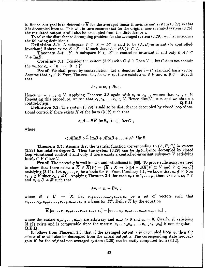
1.1 Sector region D(a,w) .......... .................................. 151.2 Inverted pendulum mounted on a platform ....... ...................... 181.3 Platform Response with Closed Loop Vibrational Control .................. 211.4 Pendulum Response with Closed Loop Vibrational Control ................. 213.1 Plant (4.1) with the augmented controller (Kom, IKQ) ..................... 343.2 Parametrized form of averaged closed loop transfer function ................. 373.3 Step Response of Averaged System ........ .......................... 403.4 Step Response of Actual System ........ ............................ 404.1 Simple model of a helicopter . . ...... .. . .444.2 (a) Altitude of helicopter in hover (1 degree of'freedom):: : . ... 524.2 b) Vertical acceleration of helicopter in hover (1 degree of freedom)......... 524.3 a Altitude of helicopter in hover (2 degrees of freedom) ................... 534.3 b Vertical acceleration of helicopter in hover (2 degrees of freedom) .......... 534.4 a Angle of the fuselage in hover (2 degrees of freedom) ................... 544.4 Anglular acceleration of the fuselage in hover (2 degrees of freedom) ...... .544.5 ertical acceleration of helicopter in hover for different a ................... 554.6 a Altitude of helicopter in flight (2 degrees of freedom) ................... 564.6 b Vertical acceleration of helicopter in flight (2 degrees of freedom) .......... 564.7 a Horizontal velocity of helicopter in flight (2 degrees of freedom) ........... 574.7 b Horizontal acceleration of helicopter in flight (2 degrees of freedom) ...... .. 574.8 a Altitude of helicopter in flight (3 degrees of freedom) ................... 584.8 b Vertical acceleration of helicopter in flight (3 degrees of freedom) .......... 584.9 a Horizontal velocity of helicopter in flight (3 degrees of freedom) ........... 594.9 b Horizontal acceleration of helicopter in flight (3 degrees of freedom) ........ 594.10 a Angle of the fuselage in flight (3 degrees of freedom) ................... 604.10 b Angular acceleration of the fuselage in flight (3 degrees of freedom) ........ 604.11 a Vertical acceleration of helicopter in flight for different a ................ 614.11 b Horizontal acceleration of helicopter in flight for different a .............. 614.12 a Altitude of helicopter in forward flight with wind gust .................. 624.12 b Vertical acceleration of helicopter in flight with wind gust .... ........... 624.13 a Horizontal velocity of helicopter in flight with wind gust ................. 634.13 b Horizontal acceleration of helicopter in flight with wind gust ............. 63

4 STATEMENT OF THE PROBLEM

The goal of this thesis is the development of a control theory for a class of dynamical systemsdescribed by the following equations:

ti(t) = Ax(t) + Bu(t)f(-). t0.1

y(t) = Cx(t),f(r) = f(r + T) , T #. 0

1ITf(r)dr =0,

0< f< 1,

where x E 1R' is the state, y E BR is the output, u E BR is the control, f(t) is a periodic,average zero scalar function, and f is a small positive parameter. Stabilizability properties ofsystem (0.1) with state and output feedback are analyzed and the pole placement capabilitiesinvestigated. A characteristic feature of system (0.1) is that the control, u, enters the openloop dynamics as an amplitude of a periodic, zero average function. Such situations arise ina number of applications where two conflicting control goals have to be accomplished by asingle actuator. For instance, in the helicopter control problem, a single actuator (the blades'pitch angle) is used to ensure both the desired altitude and the fuselage vibration suppression.These goals are conflicting in the sense that if the pitch angle is chosen to ensure the desiredaltitude, the fuselage vibrations are not suppressed; if the pitch angle is used to suppress thefuselage vibrations, the desired altitude is not attained. In order to accomplish the two goalssimultaneously, a frequency separation approach may be employed. Specifically, a low frequencycontrol may be used to stabilize the desired altitude and a high frequency, average zero controlmay be used to suppress the vibrations without compromising the first goal. When the controlloop is closed with respect to the low frequency control, the equations have the form of system(0.1), and the goal is to choose the control, u, as a function of x or y so that the resulting systemhas the desired dynamical properties.

In particular, the above ideology has been successfully implemented in the Higher HarmonicControl (HOC) of helicopters, where periodic feathering of rotor blades around a fixed pitch angleis introduced in order to suppress the fuselage vibrations. Helicopter vibration is a long standingproblem. Recent experiments [11-15] have shown that HHC may lead to an order of magnitudereduction in fuselage vibrations. The primary difficulty in implementation of the HHC systems isthe complex interaction between inertia, structural and aerodynamical hub shears and momentsfor HHC-equipped helicopter rotors. These interactions, which are difficult to predict due tothe highly complex dynamics of most helicopter systems, account for the extreme sensitivity ofHHC efficacy to proper magnitude and phasing of the HHC inputs. Using the idea of closedloop vibrational control, we will explore alternative means of suppressing the vibratory airloadwithout the phase dependencies in the input.

It is well known that unavoidable discrepancies between mathematical models and real-worldsystems can result in the degradation of control system performance. Thus, w( also investigatethe property of stability robustness for system (0.1). Both synthesis and analysis problems areaddressed. In the synthesis problem, it is assumed that (0.1) is the nominal plant, whereas thetrue plant is defined by

.i = (A+AA)x+Buf.) , (0.2)

6

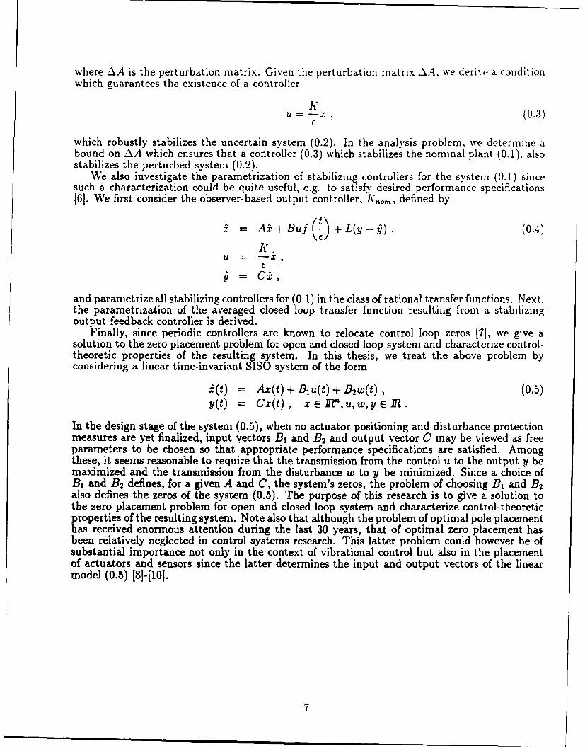
where AA is the perturbation matrix. Given the perturbation matrix AA., we derive a condition

which guarantees the existence of a controller

u = K , (0.3)

which robustly stabilizes the uncertain system (0.2). In the analysis problem, we determine abound on AA which ensures that a controller (0.3) which stabilizes the nominal plant (0.1), alsostabilizes the perturbed system (0.2).

We also investigate the parametrization of stabilizing controllers for the system (0.1) sincesuch a characterization could be quite useful, e.g. to satisfy desired performance specifications[6]. We first consider the observer-based output controller, K,,o,,, defined by

= Ai + Buf + L(y-•), (0.4)

KU =C

and parametrize all stabilizing controllers for (0.1) in the class of rational transfer functions. Next,the parametrization of the averaged closed loop transfer function resulting from a stabilizingoutput feedback controller is derived.

Finally, since periodic controllers are known to relocate control loop zeros [71, we give asolution to the zero placement problem for open and closed loop system and characterize control-theoretic properties of the resulting system. In this thesis, we treat the above problem byconsidering a linear time-invariant SISO system of the form

S= Ax(t) + Biu(t) + B 2w(t) , (0.5)y(t) = Cx(t) , z E W",u,w, y E IR.

In the design stage of the system (0.5), when no actuator positioning and disturbance protectionmeasures are yet finalized, input vectors B1 and B2 and output vector C may be viewed as freeparameters to be chosen so that appropriate performance specifications are satisfied. Amongthese, it seems reasonable to require that the transmission from the control u to the output y bemaximized and the transmission from the disturbance w to y be minimized. Since a choice ofB1 and B2 defines, for a given A and C, the system's zeros, the problem of choosing B1 and B2also defines the zeros of the system (0.5). The purpose of this research is to give a solution tothe zero placement problem for open and closed loop system and characterize control-theoreticproperties of the resulting system. Note also that although the problem of optimal pole placement

as received enormous attention during the last 30 years, that of optimal zero placement hasbeen relatively neglected in control systems research. This latter problem could however be ofsubstantial importance not only in the context of vibrational control but also in the placementof actuators and sensors since the latter determines the input and output vectors of the linearmodel (0.5) [8]-[101.

7

5 SUMMARY OF THE MOST IMPORTANT RESULTS

5.1 PART 1. STATE AND OUTPUT FEEDBACK STABILIZABILITY ANDPOLE PLACEMENT CAPABILITIES

5.1.1 INTRODUCTION

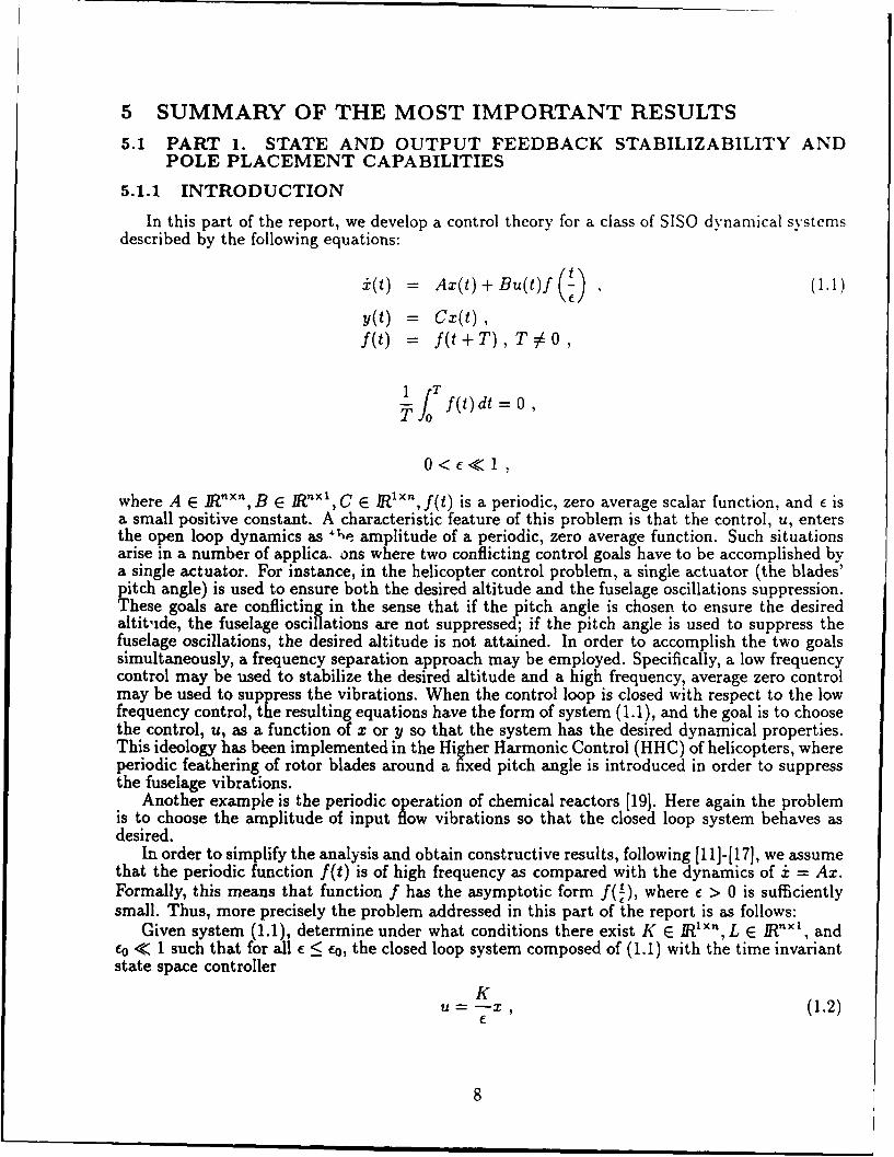
In this part of the report, we develop a control theory for a class of SISO dynamical systemsdescribed by the following equations:

i(t) = Ax(t) + Bu(t)f (D (1.1)

y(t) = CX(t),f(t) = f(t + T), T O,

Jf(t)dt = 0,

where A E RFfI Xn,B E IRxl,XC E Rlxn, f(t) is a periodic, zero average scalar function, and ( isa small positive constant. A characteristic feature of this problem is that the control, u, entersthe open loop dynamics as " amplitude of a periodic, zero average function. Such situationsarise in a number of applica, ons where two conflicting control goals have to be accomplished bya single actuator. For instance, in the helicopter control problem, a single actuator (the blades'pitch angle) is used to ensure both the desired altitude and the fuselage oscillations suppression.These goals are conflicting in the sense that if the pitch angle is chosen to ensure the desiredaltitide, the fuselage oscillations are not suppressed; if the pitch angle is used to suppress thefuselage oscillations, the desired altitude is not attained. In order to accomplish the two goalssimultaneously, a frequency separation approach may be employed. Specifically, a low frequencycontrol may be used to stabilize the desired altitude and a high frequency, average zero controlmay be used to suppress the vibrations. When the control loop is closed with respect to the lowfrequency control, the resulting equations have the form of system (1.1), and the goal is to choosethe control, u, as a function of x or y so that the system has the desired dynamical properties.This ideology has been implemented in the Higher Harmonic Control (HHC) of helicopters, whereperiodic feathering of rotor blades around a fixed pitch angle is introduced in order to suppressthe fuselage vibrations.

Another example is the periodic operation of chemical reactors [19]. Here again the problemis to choose the amplitude of input flow vibrations so that the closed loop system behaves asdesired.

In order to simplify the analysis and obtain constructive results, following [11]-[17], we assumethat the periodic function f(t) is of high frequency as compared with the dynamics of i = Ax.Formally, this means that function f has the asymptotic form f(1), where e > 0 is sufficientlysmall. Thus, more precisely the problem addressed in this part of the report is as follows:

Given system (1.1), determine under what conditions there exist K E IW", L E WC'", andco < 1 such that for all c < co, the closed loop system composed of (1.1) with the time invariantstate space controller

U = K , (1.2)

8

or a time invariant output controller

X = A- + Buf + L(y-•) (1.3)

S= Ci.

K.U = -X

is asymptotically stable. The state feedback gains of (1.2), (1.3) are restricted to be time invariantfor reasons of practical implementation. Problem (1.1), (1.2) is considered in Section 5.1.2 andproblem (1.1), (1.3) is discussed in Section 5.1.3. In addition, we characterize the pole placementcapabilities ensured by closed loop vibrational control and present the corresponding results inSection 5.1.4. To illlustrate the results, in Section 5.1.5 we consider an example inspired by ahelicopter with HHC.

5.1.2 STATE SPACE FEEDBACK

In this section, we present the result for stabilization of the system (1.1) with state spacefeedback (1.2).

Theorem 1.1: There exists a K E R"lX' and an 6o > 0 such that for all 0 < E < 60system (1.1), (1.2) is asymptotically stable if only if (A, B) is stabilizable and the sum of all thecontrollable eigenvalues of A is negative.

Proof: Necessity is proved by the following considerations. Represent the state spacemodel (1.1) in Kalman canonical form,

:i AC A12 [ ] +[ BB]juf( t ) (1.4)

where the pair (Ac, B 1) is controllable. Since Ac is not affected by feedback, the stabilizabilityof (A, B) is necessary.

The stability of xz, with xc(0) = 0, is governed by the following equation:

ac , XC E+ R m U uE1IR . (1.5)

Introducing a state feedback u = Kxc/c, we obtain

,c= [c+Bi K (1.6)

Since (1.6) is periodic, there exists a Lyapunov transformation which reduces (1.6) to an equationwith constant coefficients,

z=Az,

preserving the stability property. From the Jacobi-Liouville theorem [13],

Tj Tr [Ac+B BKf(!)dt= TrA,

9

where T is the period of f(t/c). Thus.

Tr A, = Tr A

where Tr A, is equal to the sum of all the controllable eigenvalues. Therefore. Tr A. < 0 isnecessary and this completes the proof of necessity.

Suffiency is proved as follows: Consider (1.4) and assume that all the eigenvalucs of A,, havenegative real parts. Without loss of generality, assume that (1.5) is in the controller canonicalform, i.e.:

where

0 1 ... 0 0

AC= 0 0 ... I B1 = 0

-am -am-i ... -a 1 1

and a, are the coefficients of the characteristic polynomial of matrix A,. Apply state feedback

U =" •XC L- ... ( 0 1.7)

where ki - 1, i=2, ... , m. The closed loop system is

X, = Acxc+ -BKf (1.8)

The generating equation, (17], for this system has the form

d--, = B, Kf(,r)xc, (1.10)dTr

where 7 = t/',. The general solution of (1.10) is

Xe =

where EI(r) is a fundamental matrix for BKjf(7-) and xc0 is a constant. Consequently, introducingthe substitution

x, = 4(r)ý = h(r,

we obtain the following equation in Bogoliuboff's standard form [211:

__ A] r -1f- X, (t, h(T,))(. )

- ¢-' ()AoI(r .

10

Applying the averaging principle [21], we obtain the following averaged equation

where

0 1 0

(1.13)- (C') CC/ () =0 0 ... 1 ' (.3

-a[ , - k2kml -am,- - k2k1-l• _ al

~~(~f (ffr)dT,and bar denotes the averaged value, i.e. 0(r) = 1/T for/3(r)dr. Let Ao,... I Ao,, be the open loopeigenvalues of (1.5) and choose the closed-loop eigenvalues A A,..., A, of (1.12) as follows:

I M

A, = -m. Ao, + j Im Ao, (1.14)

Then the state feedback gains (1.7) can be found to be

__(a,, - a,)ki = (a. - aI) i = 2,...,m(.5

where ac, ac. are the coefficients of the closed loop characteristic equation corresponding to.11,... , I A *.

The control gains (1.15) guarantee the asymptotic stability of the averaged system (1.12). Asit follows (17 , if (1.12) is asymptotically stable, there exists co > 0 such that for all 0 < c < coequation (1.6) is also asymptotically stable. This proves the sufficiency. Q.E.D.

Corollary 1.1: Assume that the sum of the controllable eigenvalues of A in (1.1) ispositive, then there exists an fo such that no dynamic state feedback of the form

ý = Fv+Gx , (1.16)1

u = -[Hv+Jx]

will stabilize the system (1.1) whenever 0 < c < co.Proofh The resulting closed loop equations with the dynamic state feedback controller

(1.16) are:

i = Ax+B HLVf(!+ B iXf(

v = Fv+Gx.

In fast time r = t/O, the above equation becomes:

[•1_ = [ EA+BJf(r) BHf~r)J] F (1.17)

liIV cG F V1.7

Let 4b(r) be a fundamental matrix for BJf(-r). Define

W = j t(r - q)BHf(q)dq.

and the substitution

v(r)]=[ 0 I

Using the above substitution, we obtain

A111 A~ - ýD1 WG4D ýD'AW - 4ý'WGW - 4"'WF(1)1,,, G4DGW+F

which is an equation in the standard form [21]. Introduce the following Lyapunov transformation

z2(t) I0•(t)

which will preserve the stability of (1.18), yields

Applying the averaging principle [21], we obtain

Thus the eignevalues of the averaged closed loop system are the union of those of -1 AD and F.It follows from Theorem 1.1 and the averaging principle [211, that if Tr A > 0, there exists an cosuch that the closed loop system (1.1), (1.16) will be unstable whenever 0 < E _< cE. Q.E.D.

5.1.3 OUTPUT FEEDBACK

This section deals with the problem of stabilizing system (1.1) with an output feedback (1.3).Theorem 1.2: There exists a K E RX"',L E Rr'l, and an co > 0 such that for all

0 < c < f0 the system (1.1), (1.3) is asymptotically stable if and only if (A, B, C) is stabilizableand detectable and the sum of the controllable eigenvalues of A is negative. The separationprinciple holds, i.e. the choice of K and L can be carried out independently.

Proof: Necessity is proved by the following considerations. Consider the observer,

S= Ai + Buf + L(y - C- )

and the feedback law

KU = -" X .

The dynamical equations for the closed loop system are:

12

A Bjf 1 x[] [ ( LC+ f31x] (1.19)S= LC (A4- LC)+B f f

Defining the observation error e = x - i. we obtain the following equivalent dynamical equations:

(A -LC) I [ I]Thus, the stability of the closed loop system depends on those of A+ (1/e)BKf(t1f) and A - LC.Using the results of Theorem 1.1 completes the proof of necessity.

Sufficiency is proved as follows: Consider system (1.1) with (A, B, C) stabilizable and de-tectable. In fast time r = t/f, the resulting closed-loop equations with output feedback (1.3)are:

E•, = cLC E(A- LC) + BKf(r) i(

Let P(r) be a fundamental matrix for BKf(7). Define

,()= 4- 1 (T)A4(T),

and the substitution

x(r) 1 [I BK fo(q)f(q)dq [(T):i(r) =[ BK o N() I I W(r)I,

Using the above substitution and following the proof of Theorem 1.1, we reduce (1.20) to thestandard form [21] and apply the averaging principle to obtain the following averaged equations:

[ [A +TLC -LCT i- A +LC -TLC] ] (1.21)

To simplify (1.21), introduce the following transformation

which yields

[Z2 L~ 0 iA-LC+ILC 2ji (1.22)

Using a construction similar to that of (1.10)-(1.12), one can compute the state feedback gainrequired to stabilize f, and assign all the eigenvalues of A - LC through the choice of L so thatthe asymptotic stability of (1.21) is guaranteed. As it follows [17), if (1.21) is asymptoticallystable, there exists an f0 > 0 such that for all 0 < e < f- equation (1.19) is also asymptoticallystable. Q.E.D.

13

5.1.4 POLE PLACEMENT CAPABILITIES

Consider again system (1.1) with feedback (1.2) and assume that

where k/ ,-' 1, i = 1,..-.,n. Thus, the closed loop system is

As it is shown in [171 and (1.12), this equation can be reduced to the averaged equation,

(A B (1.24)

where

x(r) =

.(r) is a fundamental matrix for BKf(r) and r = t/E. As it follows from [17) and [21], (1.23)is asymptotically stable for sufficiently small E if the averaged system (1.24) is asymptoticallystable. Matrix R which, along with matrix A, defines the stability of (1.24) can be characterizedas follows:

Theorem 1.3: Assume A and B are in the controller canonical form. Then there existsf- such that for all 0 < c < co, matrix B of (1.24) has the form:

0 ... 0 0

= 0 ... 0 0 (1.25)

and00 2 k2 ki

where a, s 1, 2,..., are the Fourier coefficients of f(r), i.e.

00

f(r) - a, sin(sr + (p.)

Proof: Follows directly from Theorem 3 of [13].

Denote the characteristic polynomials of A and (A +W) of (1.23) and (1.24), respectively, by

Po(s) = sn + a1os-' 1 + a2osn 2 + .- + ao, (1.26)p(s) = sn +asn- 1 + a 28n-2 +. +a, . (1.27)

It follows from Theorem 1.3 that

a, alo , (1.28)a 2 _ a20 , (1.29)

14

Im X

D~a, a

Re•X

Figure 1.1: Sector region D(o,w)

and aj, 3 < j <_ n, can be arbitrarily assigned. Below we analyze to what extent the constraints(1.28) and (1.29) prevent the control designer from assigning the closed loop eigenvalues of theaveraged equation (1.24) to a desired region of the complex plane.

More specifically, considering the closed region D(a, w) of Figure 1.1, our purpose is to identifythe conditions under which we can find n real or complex numbers An,..., A,, occurring as pairsof complex poles, such that they are the roots of the polynomial (1.27) which satisfy (1.28) and(1.29). When this is possible, we say that (real or complex) pole assignment in the region D(a, W)using closed loop vibrational control is possible. Note that if the closed loop poles are confinedto this region, then the system modes of (1.24), and hence the averaged modes of (1.23), willhave a time constant smaller than or equal to -1/la and decay exponentially at a rate greaterthan or equal to -a/v'/2 -+w2 .

Since, closed loop vibrational control can only modify the coefficients a,0 , 2 2. Lemmas A.1-A.5 are contained in AppendixAl.

Theorem 1.4: Pole assignment in the region D(a, w) using closed loop vibrational controlis possible, only if

-al 0 n_ v. (1.30)

15

Proof: If A1,... \A E D(a,w) are the roots of the polynomial (1.27). then

-a = A, (1.31)s=l

andRe(A,) _< a. (1.32)

Equation (1.30) is obtained by equating the real parts in (1.31) and using(1.32). Q.E.D.

Theorem 1.5: Real pole assignment in the region D(a,w) is possible using closed loopvibrational control feedback if and only if

-al 0 _< no, (1.33)n-i~ 2

a20 <_ a 2 (1.34)

Proof. The necessity of (1.33) follows from Theorem 1.4. The necessity of (1.34) followsfrom the fact that when A1,..., A,, are the roots of (1.27), the coefficients a, and a 2 are

n

a,- -= A (1.35)i=1

a 2 = Z A, Aj. (1.36)

i>J

The maximum value that (1.36) can achieve subject to the constraint (1.35), (1.28) is given byLemma A.2 and is exactly the right hand side of (1.34). Therefore if (1.34) is violated, poleassignment to the region D(o, ,) with real poles is not possible.

To prove ýhe sufficiency of (1.33), (1.34), assume they both hold. Choose

a l 0l = ... =A = n-

It is immediately checked that these real numbers solve the problem of pole assignment to theregion D(o, w), which completes the proof. Q.E.D.

Theorem 1.5 gives a simple solution of the problem of pole assignment to the region D(a,w)with real poles. When complex poles are allowed, results similar to Theorem 1.5 are obtained:

Theorem 1.6: Complex pole assignment in the region D(o-, w) is possible using closedloop vibrational control feedback if and only if(i) for n even

-aJo •_ no', (1.37)

and

a20 < aio ((n - 1)a2 +w2), (if Io"I>w) , (1.38)

or

- (w2 _a2) (n'- 2) (n+ ++ (2 ,2) (a°) (if H <w), (1.39)

16

(ii) for n odd with one real pole placed at p < a

-alo •_ (n-1)a+p, (1.40)

and

a20 .5 p(ao+(p)a+2(-+P) 2 ((n - 2)a2 2) (if Ia > w) (1.41)

or

a 20 :5 -p(aio + p) + (w-2 _ a2) (n- ) (n--I + aao+)p

2 2 aP 2+(W2 + a'2 ) 2u+ (if Io< <w) (1.42)

Proof: We first consider the case when n is even and let Ija > w. The necessity of (1.37)follows from Theorem 1.4. The necessity of (1.38) follows from the fact that when A,,..., A,, arethe roots of (1.27), the coefficients a, and a 2 are

na1 = (1.43)

i--1

a 2 = ZA1 A. (1.44)

i>3

The maximum value that (1.44) can achieve subject to the constraint (1.43), (1.28) is given byLemma A.2 and is exactly the right hand side of (1.38).

To prove the sufficiency of (1.37), (1.38), assume they both hold. Choose

A; = -ýý- i~(1 = 1...,nna(a (

It is immediately checked that these complex numbers solve the problem of pole assignment tothe region D(a,w), which completes the proof.

When n is even and Jal< w, the proof is similar and follows immediately from Theorem 1.4and Lemma A.3.

The proof for the case when n is odd is completed by using Theorem 1.4, Lemma A.4 (ifJal > w) and Lemma A.5 (if Jal < w). Q.E.D.

Remark 1.1: If a2 -w2 = 0, then conditions (1.38), (1.39) and (1.41), (1.42) in Theorem2.6 are identical. Note also that the expressions in the right hand side of (1.39) and (1.42)have larger values than the corresponding expressions in the right hand side of (1.38) and (1.41)respectively. Consequently, it is easier to satisfy the condition for assigning complex poles intothe region D(a, w) such that ,2 -_w2 < 0 with closed loop vibrational control.

Remark 1.2: Some observations concerning the region D(a,w) are in order. Let A =-Cw,, +- jwd be a complex pole, where C is the damping ratio, 0 < C < 1,w, = JAI is thenatural (undamped) frequency, and wd = w,,/'' is the damped natural frequency. Then ifA E D(a,w), it follows that C > -al/v/2 -+w2 and -Cw,, < a. To analyze the pole placementcapabilities of the closed loop vibrational control, we note that in practice, design specifications

17

F/2 I0 F/2zl4i M

Figure 1.2: Inverted pendulum mounted on a platform

are often given in terms of _,.,, and -Cw,, < a. Such specifications will be satisfied byD(o,, w) if a < a and -W/-2 + >2 _ mm, or equivalently

a < a, (1.45)W < -a _ 1 (1.46)

Hence, different values of a and w, subject to the constraints in Theorem 1.6, can be chosen toenforce different bounds on the damping ratio, natural frequency and damped natural frequencyof the averaged closed loop system.

5.1.5 AN ILLUSTRATIVE EXAMPLE

Below we present an example inspired by a helicopter with HHC. The system is shown inFigure 1.2. Here, an inverted pendulum is mounted on a platform, and the goal is to maintainthe platform altitude at the desired level, z = 0, and the pendulum at the upright position, 0 = 0,using a single force actuator, F, located on the platform. The two goals are clearly conflictingin the sense mentioned in Section 5.1.1. Specifically, if we use the actuator to maintain theplatform at z = 0, the pendulum will topple down; if we use the actuator to force the platformto move with an acceleration lesser than -g, the pendulum will stay in the upright position butthe platform will not be at z = 0. Therefore, closed loop vibrational control is the method ofchoice.

The Lagrange equations for the system at hand are:

(Mi + m 2 )., - m 21sin0 - m 2 12 cosO + (Mi + m 2 )g = F - , (1.47)

m212j - m2 /(, + g)sin0 = -ri, (1.48)where ml, z and C denote the mass, altitude and damping coefficient of the platform, m 2,0, 1,and q represent the mass, angle, length and damping coefficient of the pendulum. Following theideology of closed loop vibrational control, we choose F with frequency-separated components:

F = (m+ M2)- kz + -f1 (1.49)

18

Here the first term compensates in an open loop fashion for the system's weight, the second termis the low frequency feedback to maintain z = 0, and the third term is the high frequency controlto maintain 0 = 0.

To reduce (1.47), (1.48) to the form (1.1), we linearize all the nonlinearities in (1.47) and(1.48) retaining, however, the interaction term iB in (1.48). Assuming that f1 (t/c) = sin(t/c),solving (1.47) as t --+ oc and substituting the resulting periodic function in (1.48), we obtain asystem of the form (1.1) with

X A 0 J!, B C O 1 0 f si

andU= K (1.50)

where

K = [l(M 0 J (.

and 0 is the phase shift introduced by the system (1.47) with input f1 (t/E). Since Tr A < 0 and(A, B) is controllable, according to Theorem 1.1, there exists an co such that for all 0 < f _< o,the system (1.50) is stabilizabletby a state space feedback. Since, in addition, (C, A) is observable,the system is stabilizable by output feedback as well (Theorem 1.2).

Further according to Theorem 1.5, real pole assignment in the region D(, ,w) is possible ifand only if

2m2> -r (1.52)- 2M212

-..9 < 11 2

I - 4m2l24

The second condition is always met. Therefore, for real pole assignment, a has to be chosenso that the condition (1.52) is satisfied.

According to Theorem 1.6, complex pole assignment into the region D(a, W) is possible if andonly if (1.52) is met and, in addition,

-_g< M1a(a+ W21 - 4mnl4 r2

is satisfied. Again, since the last condition is always satisfied, (1.52) is necessary and sufficientfor both real and complex pole assignment in D(a, w).

To design a specific controller for (1.47), (1.48), we average equation (1.50) to obtain

0a10,2 51r

212 (m1+M2) 2 M JThen, if we choose the closed loop poles at

Al, = A2 = 12

19

the resulting control gain K is given in (1.51) with

o= slmIr m ) +r + (1.33S(1.53)

In general, if (1.52) is met, the gain K that assigns the closed loop poles at A1, and A2,, isexpressed by (1.51) with:

c = v'2l(ml + in 2 )- A 2 +. (1.54)

If we choose the observer gain L = [1I 121 to ensure that the observer poles are at

A,, = A2o = -yA1 , = 772r >0,

then

11 (77M2 12

12 = (7+2)2172 g4m~l4 +7

In general, the observer gain L that assigns the observer poles at A1,, A2o is given by11 = -A,. - A2 . -7

12 = AmoA2, -'l 2 +

Mrn2 2 1

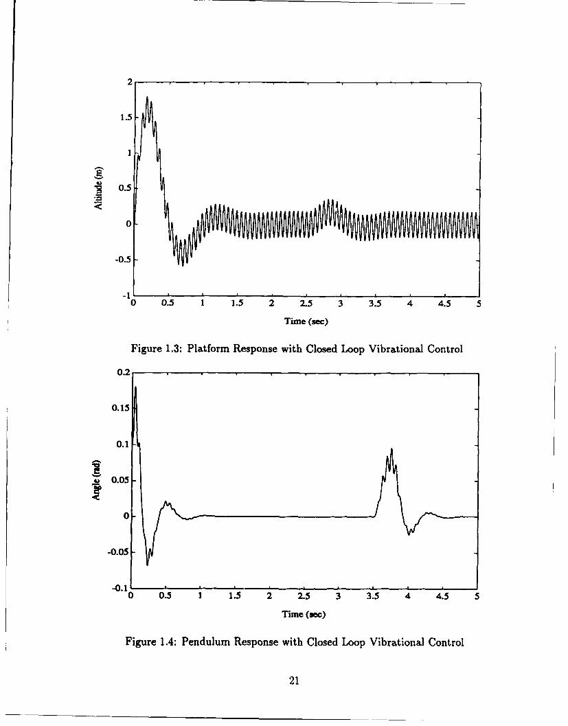
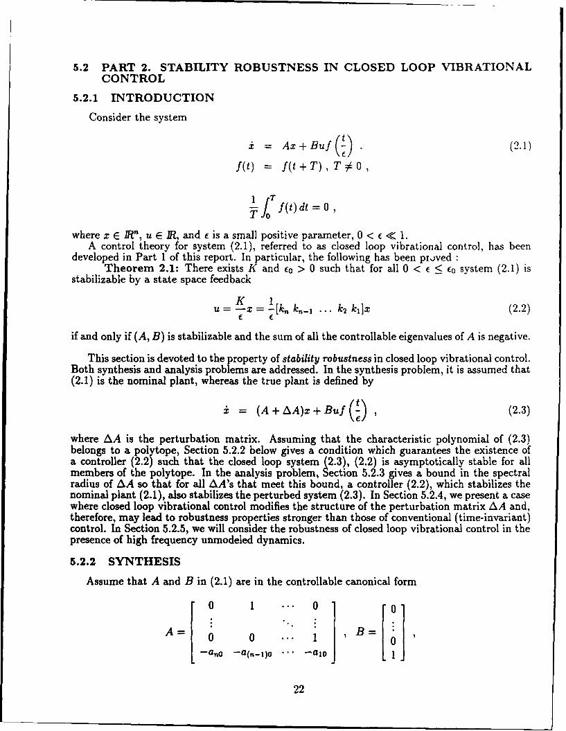
To illustrate the behavior of the pendulum-platform system with closed loop vibrationalcontrol, we carried out numerical simulations of equations (1.47), (1.48) with the following pa-rameters : MI = 0.1 kg, m2 = 0.01 kg, g = 9.8 m/s 2, 1 = 1 m, 77 = 0.1, C = 0.6. The controllaw has been chosen as in (1.49) with k = 5,a = 2 (see (1.54)) and e = 0.01. The results areillustrated in Figures 1.3 and 1.4 for the initial conditions z = 0 m and 6 = 0.1 rad. In addition,we introduced impulsive perturbations at the platform (at t 2.5 sec) and at the pendulum (att = 3.5 sec). As it follows from these graphs, the closed loop vibrational control indeed ensures,on the average, simultaneous satisfaction of the two conflicting objectives using a single actuator.Note that the limit cycle in the dynamics of the platform is due to the fact that the controller(1.51), derived for the linear system (1.1), (1.50), is, in fact, applied to the original nonlinearsystem (1.47), (1.48). This is why closed loop vibrational control may lead to the satisfaction ofthe two conflicting goals not pointwise in time but only on the average.

20

2

1.5

" 0.5

0

-0.5

-10 0.5 1 1.5 2 2.5 3 3.5 4 4.5 5

Time (sec)

Figure 1.3: Platform Response with Closed Loop Vibrational Control

0.2

0.15

0.1

S0.05

0-

-0.05

-0.1 L0 0.5 1 1.5 2 2.5 3 3.5 4 4.5 5

Time (sec)

Figure 1.4: Pendulum Response with Closed Loop Vibrational Control

21

5.2 PART 2. STABILITY ROBUSTNESS IN CLOSED LOOP VIBRATIONAL

CONTROL

5.2.1 INTRODUCTION

Consider the system

SA x + B uf ) . (2.1)

f(t) = f(t+T), T#O,

T f(t)dt =0,

where x E Rn, u E IR, and c is a small positive parameter, 0 < c « 1.A control theory for system (2.1), referred to as closed loop vibrational control, has been

developed in Part 1 of this report. In particular, the following has been proved :Theorem 2.1: There exists K and co > 0 such that for all 0 < ( < co system (2.1) is

stabilizable by a state space feedback

K 1u = -X = -I[k k,n- 1 ... k2 kj]x (2.2)

f f

if and only if (A, B) is stabilizable and the sum of all the controllable eigenvalues of A is negative.

This section is devoted to the property of stability robustness in closed loop vibrational control.Both synthesis and analysis problems are addressed. In the synthesis problem, it is assumed that(2.1) is the nominal plant, whereas the true plant is defined by

i = (A+AA)x+Buf(!) , (2.3)

where AA is the perturbation matrix. Assuming that the characteristic polynomial of (2.3)belongs to a polytope, Section 5.2.2 below gives a condition which guarantees the existence ofa controller (2.2) such that the closed loop system (2.3), (2.2) is asymptotically stable for allmembers of the polytope. In the analysis problem, Section 5.2.3 gives a bound in the spectralradius of AA so that for all AA's that meet this bound, a controller (2.2), which stabilizes thenominal plant (2.1), also stabilizes the perturbed system (2.3). In Section 5.2.4, we present a casewhere closed loop vibrational control modifies the structure of the perturbation matrix AA and,therefore, may lead to robustness properties stronger than those of conventional (time-invariant)control. In Section 5.2.5, we will consider the robustness of closed loop vibrational control in thepresence of high frequency unmodeled dynamics.

5.2.2 SYNTHESIS

Assume that A and B in (2.1) are in the controllable canonical form

0 1 0 02

A= 0 0 ... 1 B=

-ano -a(,n-1)o .. .alo1

22

where aj0 are the coefficients of the characteristic polynomial of the nominal system (2.1). Assumethat the perturbation matrix AA affects the last row of the system matrix A. and that thecharacteristic polynomial of the perturbed system (2.3) belongs to the class P defined as follows:

P (=p(s) aEjPj(S):ao ,j-1,...,m;E a- =1j=--1 j=1

Here

p,(S) = s + a',S"-1 + ... + a),j= 1,...,m ,(2.4)

are the vertex polynomials and ai,,i = 1,...,n denote the ith coefficient of the Jth vertexpolynomial.

Theorem 2.2: There exists K and fo such that for all 0 < e < co, any perturbed system(2.3) with open loop characteristic polynomial in P can be stabilized by a single controller (2.2)if and only if all coefficients ai,j = 1,... , m, defined in (2.4), are positive.

The proof of Theorem 2.2, is based on the following lemmas:Lemma 2.1: [61] Consider a polynomial

p(S) = s + ,n-I +... + on, ,(2.5)

where n > 3, ip > 0,i = 1,... ,n. Let 6 be the positive real solution of the equation 6(6+ 1)2 = 1.Then polynomial (2.5) is Hurwitz if the coefficients hik satisfy the condition

l=t-10+2 < 1,...,n - 2 . (2.6)0101+1 -

Inequality (2.6) will henceforth be referred to as the Lipatov's conditon [61].Lemma 2.2: Consider the following four polynomials:

Pkl(s) = s++ ' n- + Y+S- + s-3 + YS'-4 + ... (2.7)Pk2(S) = Sn + sn-1 + Y sn-2 + Y3+ "-3 + -4+s"-4 +

pk3(S) = Sn +-Yjs- 1 +-t,+sn-2 +-tSn-3 +,Zn- 4 +...

pk4(S) = Sn + -_YSn-"2 s + -f"s-n 3 +-+ 74- 4 +...

where n > 3, 7 - , 1 0. Let coefficients T, 1 0. Then there exists a k* such that for all 0 < k < k', the coefficient T2 is positiveand the polynomials

pk, I+(s) = sn + (-I+ + -"(k))s"- + (y + U--(k))s'- 2 + ( 3y + "(k))s- 3 +... (2.9)

pk12(S) = S'+ + + + (k))Sn- 1 + (Y-f + W(k))Sn-2 + (f+ + 3(k))s"-3 +...pk 3(S) = s,+ + + Ui(k))s-' + (-+ + W2(k))s'- 2 + (+ + "i(k))s- 3 +...

Pkd,4(S) = ?+(7+ + T(k))s"- + (-t + 7(k))s"- +(7; + (k))s"- +...

are Hurwitz.

23

Proof: Let - denotes the ith coefficient, 1 < i < n, of the jth polynomial. I <j < 4, in(2.7). First, we show that there exists k* such that for all 0 < k < k-, polynomials (2.9) satisfyLipatov's condition, i.e.

max (-, + - +2 +--((k)) k 6 < (2.10)

'1'51<n-'2<' (<' + + a--+, (k))

where 6' is defined in Lemma 3.1. Then, the statement of this lemma follows directly fromLemma 3.1. To show that Lipatov's condition holds, consider

f =(k) max + 7:T(kD(-i+ 2 +aj-2 (k)) 1 << n -2. (2.11)'_<j:_4 (-ý + Tj(k)) (-?+I + T-+-•(k))

It is easy to see that the function f1 (k) is monotonically increasing with respect to k. Indeed,define W0(k) = 0 and -1o = -+ = 1. Let c+ (k) = 1+ + U(k), c- (k) = 7 + T(k), and Atc.c+ (k) - c- (k) =-y+ - - for 0 < q < n. Then

I- 1(k)c+2 ( k)__fj (k) = + +'(kc 1( 1 < I < n - 2 ,(2.12)

cji(k)cI, (k) +cT(k)c•4(k) Ac +_----(,

= ..(k) 1+ ( + 1\-kc c1(k) C 12k

where

(k= k , if2 0, and since c,(k) = 7, + i(k) for 2 0 for 0 < q < nand from (2.14), 0(kj) < O(k 2 ) for 0 < k1 < k2 . Thus, f1 (k) is a continuous and monotonicallyincreasing function of k. Also, as it follows from (2.13), f(O) = 0, and limrk_oo f1 (k) = oo.Therefore, by the intermediate value theorem, there exists kT* such that

f 1(kfl) = 6, 1 < I < n - 2. (2.15)

Let k* = mint kt*. Since f1(k) is monotonically increasing with k, it follows that f1(k*) <fi(kT), 1 0, i.e.

k'--n > 0, (2.16)

choose k in (2.8) as follows:

24

(i) if •< 0,1let 0 < k< k'(ii) if -y >0 , let 0 < k < min[(t)---, k] . Q.E.D.

Proof: (of Theorem 2.2) Consider the closed loop system (2.3), (2.2) :

± = (A+AA+BA A f( )). (2.17)

In the fast time r = t/c, the closed loop system (2.17) is

dx- = (((A + AA) + BKf(r))x . (2.18)

Let O(r) be a fundamental matrix for BKfJ(r). Reducing (2.18) into the standard form [21] andthen applying the averaging principle, we have the following averaged system

x= 4-(!(A+ A)(! T, (2.19)

where the bar denotes time averaging operation. According to Theorem 2 of [171, there existsco such that for all 0 < c < co, system (2.17) is asymptotically stable if the averaged system(2.19) is also asymptotically stable. Moreover, it was shown in [52] that the averaged closed loopsystem (2.19) has the following characteristic polynomial:

PCI(s) = s' + (a, + "-))s"-' + (a 2 + 2 +... + (a, + "-) , (2.20)

where

a- = k2ks-? , i = 1,...,n , (2.21)ki = 0,

I.t

0(t) = J0 f(r) dr,

and the coefficients ai are the coefficients of the characteristic polynomial of the perturbed system(2".'he necessity part is obvious: Since the a, coefficient in (2.20) cannot be adjusted, it isnecessary that aj > 0,j = 1,... , m for (2.20) to be Hurwitz.

Sufficiency is based on Kharitonov's theorem [58] and Lemma 3.2. For 0 < n < 2, it is easyto construct W, 1 _ i < n to stabilize (2.20). Hence, we will consider the case when n > 3.Let -i- = minja•, 7+ = maxi a4, where a; denotes the ith coefficient, 1 < i < n, of the jthvertex polynomial 1 < j < m. We first construct four interval polynomials which contain thepolynomial (2.20):

Pkd S) = " n-1 + 4Sn-2 + .- 3 +c-,n4 +

pdJ2(S) = s" +cI' 1 + qs- 2 +4s"-3 + 4+sn- +...

Pk,13(S) = n- + CSn--1 + C4!Sn2 + 4S-n3 + C4 S + ...pd4(S) = •n + C+ "n-1 + -n-2 + ;Sn-3 + C4+Sn-4

(2.22)

where

c7 + i < n (2.23)•,+= t + U;

25

Next, we need to determine U in (2.23) satisfying a- = 0. > 0 so that the four intervalpolynomials (2.22) are Hurwitz. It follows from Kharitonov's theorem that if the polynomials(2.22) are Hurwitz, then (2.20) is also Hurwitz. Choose _,, I < i < n as defined in (2.S).then from Lemma 3.2, there exists a k such that for all 0 < k < k", polynomials (2.22) areHurwitz. The corresponding stabilizing state feedback gain K can be computed from (2.21).As it follows [17], for each Hurwitz averaged closed loop polynomial pci(s) in (2.20) there existscp > 0 such that for all 0 < _< f, the corresponding closed loop system of (2.3), (2.2) is alsoasymptotically stable. In [17), a lower bound of cp was derived. This bound for c, is a continuousfunction of the coefficients of the open loop characteristic polynomial p(s). Since the set of openloop characteristic polynomial p(s) E P is closed and bounded, it follows from the property ofcontinous functions that a uniform lower bound of fp exists. The proof is completed by settingco = minp fp. Q.E.D.

Remark 2.1 : The condition that the coefficient a, > O,j = 1,... , m, in Theorem 2.2 isequivalent to the requirement that the trace of the perturbed matrix A + AA be negative.

Remark 2.2 : Theorem 2.2 is an extension of the result obtained in [62] for interval poly-nomials. The assumption that P is polytopic is weaker than Kharitonov's interval polynomialassumption because it allows for linearly dependent coefficient perturbations.

Example 2.1 : Consider a 6th order system (2.3) with open loop characteristic polynomialp(s) E P where P is a polytope of polynomials (convex hull) with the following four vertexpolynomials

pi(s) = s6 + 0.5s5 - 0.6s 4 + 1.5s3 + 2.5s2 +3.4s-3 ,p2 (S) = S6 +0.7s5 - S4 +2S3 +2s 2 +4s - 1p3 (s) = 6+S5+S4 +S +3s 2 +3s+1,

P4(S) = S6 + 0.6s5 + 0.2s4 + 1.13+2.9s2 +3.8s+22

This uncertain open loop system is unstable since the vertex polynomials pi(s) and p2(s) areobviously unstable. With vibrational state feedback control (2.2), the characteristic polynomial(2.20) of the resulting averaged closed loop system is bounded by the interval polynomials (2.22).Next, we construct a-i, I 0 so that the intervalpolynomials (2.22) are Hurwitz. Following (2.12), we define the function f,(k) as:

ft(k)= ci_7(k)c 1+2(L) 1 < 1 < 4C7 (k) c- I(k)

and hence

f,(k ) - k3 "5 ( + ^1 T ,

f 2 (k) = k ( + -) (1 +

f3 (k) = k (1 + Ac2 k5) + Ac-k

f 4 (k) = k (±1 + ) + Ac 6k4

where Ac, = c- c, max al- min 4, Consequently, with -j =minj a= 0.5, 6 = 0.4656,we compute kT, 1 < 1 < 4, such that

fl(k*) = (k•') 3 ,5 (l + 2(kl*)'' 5 ) = *', (2.24)

26

f 2(k;) = k;(1 + 1)(1 + (k; = ', (2.25)

f 3(k;) = k;(1 + 2(k;)5 )(1 + 2k) =6 , (2.26)

f 4(k:) = k:(1 + 2(k;)'"s)(1 + 5(k;) 4) = 6• (2.27)

Solving (2.24)-(2.27), we obtain k = 0.6536, k; = 0.2327, k- = 0.2925, k: = 0.3232. Thus k =

mint kT* = k2 = 0.2327. Since mini a2 < 0, for 0 < k < 0.2327, the interval polynomials (2.22)and consequently, the characteristic polynomial (2.20) will be stabilized. Arbitrarily choosek = 0.23, then U2 = 1554.7,T = 3.5, T4 = 3237.6, Ts- = -0.8, and T = 360.3. With f(r) = sin r,the corresponding feedback gains in (2.2) was k, = 0, k2 = 55.8, k3 = 0.1255, k4 = 116.1,k 5 =

-0.0287, and k6 = 12.9. The stability of the characteristic polynomial (2.20) of the averagedclosed loop system with the feedback K, can be verified by performing eigenvalue tests onappropriate Hurwitz matrices corresponding to each of the vertices of the polytope of polynomialsP (63]. From Theorem 2 of [17], the asymptotic stability of the averaged closed loop system willensure the asymptotic stability of the original system (2.3).

5.2.3 ANALYSIS

Consider system (2.3) with feedback (2.2):

i = (A+ A±BK f ()) (2.28)

Assume that K and c are chosen according to Theorem 2.1 so that (2.28) is asymptoticallystable when AA = 0. Under this condition, we obtain the following results:

Theorem 2.3: There exists fo such that for all 0 < c < fo, the system (2.28) is aymptot-ically stable if

O'mox 'I- (- iA5 (D • Ai(Q) (2.29)( If ) () Ar ,.(P)I

where P is the unique positive definite solution of the Lyapunov equation

PA+ AP+2Q = 0, (2.30)

Q is some positive definite matrix and

A t -1(A)O(A (2.31)

Proof: From (2.19), the averaged closed loop system's equation of (2.28) is:

X 4b1 .1(A +AA)$()

=(A + A-A) 7, (2.32)

where

= 5-= (- ) AAS A)

and the bar denotes time averaging operation.

27

Note that (2.32) is obtained by the linearity of the averaging operation. From [67]. we knowthat the averaged linear time-invariant system (2.32) is stable if

amar(AA) < A""',(Q) (2.33)Amaz(P) *

where P is the unique matrix that satisfies the Lyapunov equation (2.30). Q is any positivedefinite matrix and o...(M) represents the largest singular value of l.

Hence, for each AA satisfying (2.29), the averaged system (2.32) is asymptotically stable,and there exists fAA such that for all 0 < f < f&AA, system (2.28) is also asymptotically stable.In [171, it was shown that CAA is a continuous function of the elements of the matrix AA. Sincethe set of AA satisfying (2.29) is closed and bounded, it follows that there exists a uniform lowerbound for CA. The proof is completed by setting fo = min&A CAA. Q.E.D.

Note that the perturbation bounds given by (2.29) are indirectly imposed on ZAA throughthe averaged perturbed matrix AA. Assume that A and B are in the controller canonical form,then

AA = AA+ AA, (2.34)

where

0 ... 0 0

AA= 0 00 0 (2.35)

Sk, - Ainkn-i+- ... k2 , -0 Jand AAij denotes the (i,j)th element of the perturbation matrix AA.

Corollary 2.1: Assume that A and B are in controller canonical form. Then there existsan f- such that for all 0 < e < c, the system (2.28) is stable if

Amn( Q) (.6amax(AA) + am,,(AAI) < Amin,(P) (2.36)

Proof: The proof follows directly from Theorem 2.1, (2.34) and the fact that aO,,L(AA +AA1 ) _ a,..m(AA) + a0 .(AA 1 ). Q.E.D.

Example 2.2 : Consider the system (2.28) with

A = [ -3 ,B 1 , Bf (r) =sin(r),

and K = [2 0]. Applying the averaging principle, we obtain the averaged system (2.32) with

1 -2 -3

Choose Q = I. From (2.36), the allowable range of the perturbation matrix which ensures theasymptotic stability of the original system (2.28) is given by

Umaz(AA) + 21AA1 21 5 0.382

28

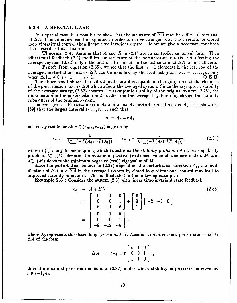
5.2.4 A SPECIAL CASE

In a special case, it is possible to show that the structure of _A may be different from thatof AA. This difference can be exploited in order to derive stronger robustness results for closedloop vibrational control than linear time-invariant control. Below we give a necessary conditionthat describes this situation.

Theorem 2.4: Assume that A and B in (2.1) are in controller canonical form. Thenvibrational feedback (2.2) modifies the structure of the perturbation matrix AA affecting theaveraged system (2.32) only if the first n - 1 elements in the last column of AA are not all zero.

Proof: From equation (2.35), we see that the first n - 1 elements in the last row of theaveraged perturbation matrix AA can be modified by the feedback gains ki, i = 2. ... , n, onlywhen AA # 0,j = 1,...,n - 1. Q.E.D.

The above result shows that vibrational control is capable of changing some of the elementsof the perturbation matrix AA which affects the averaged system. Since the asymptotic stabilityof the averaged system (2.32) ensures the asymptotic stability of the original system (2.28), themodification in the perturbation matrix affecting the averaged system may change the stabilityrobustness of the original system.

Indeed, given a Hurwitz matrix Ao and a matrix perturbation direction A,, it is shown in[69] that the largest interval (rmm, rmaz) such that

Ar = Ao + rA 1

is strictly stable for all r E (rmin, rnmt,) is given by

1 1

= A~i,(-T(Ao)- 1 T(Aj)) , = A+.(-T(Ao)- 1 T(Ai)) , (2.37)

where T(.) is any linear mapping which transforms the stability problem into a nonsingularityproblem, A)+..,(M) denotes the maximum positive (real) eigenvalue of a square matrix M, andA i-(M) denotes the minimum negative (real) eigenvalue of M.

"'ince the perturbation bounds in (2.37) depend on the perturbation direction A,, the mod-ification of AA into TAi in the averaged system by closed loop vibrational control may lead toimproved stability robustness. This is illustrated in the following example :

Example 2.3 : Consider the system (2.3) with linear time-invariant state feedback

Ao = A+BK (2.38)

0 [ [ 2 -1 0S0 0 1 0 J- 01 1

-6 -11 _6 1

0 1 0[0 0 1

-8 -12 -6

where Ao represents the closed loop system matrix. Assume a unidirectional perturbation matrixAA of the form

0 1 0

AA = rA 1 =r 0 0 19• 1 0

then the maximal perturbation bounds (2.37) under which stability is preserved is given byr E (-1,4).

29

Next, we consider the same open loop system (2.3) with f(r) = sin r and introduce closedloop vibrational feedback of the form (2.2). Choose K = [2v.2 v'2 0] so that the averagedclosed loop matrix A in (2.32) is identical to A0 . This ensures that the dynamics of the system(2.3) with closed loop vibrational control is similar to the linear time-invariant state feedback(2.38). Then AA in (2.32) will have the form

0 1 0A-A = r 0 0 1

0 0 1

From (2.37), we determine system (2.32) is stable if and only if r E (-1, 8), which compares fa-vorably with the interval (-1,4) obtained for linear time-invariant state feedback. Unfortunately,this situation does not always take place:

Example 2.4 : Consider the same nominal closed loop system as in Example 2.3. However,assume that AA now has the form:

0 1 0

AA= r 0 0 1

Then with linear time-invariant state feedback (2.38), the maximal range which ensures thestability of the closed loop system is r E (-1,4).

With closed loop vibrational feedback (2.2), the averaged perturbation matrix 'A becomesS0 1 01

AA = r 0 0 10 - 1 1

and closed loop stability of the averaged system is ensured if r E (-1, 3.6298).

5.2.5 UNMODELED DYNAMICS

Generally, a model of the system to be controlled may become less accurate at high frequenciesbecause of unknown or unmodeled parasitic dynamics. Moreover, these parasitic dynamics maychange with time or other physical parameters, and so cannot be confidently modeled.

In state space plant descriptions, the addition of high frequency parasitic dynamics is calleda singular perturbation, because the perturbed plant has more states than the plant. Considerthe following singularly perturbed form of (2.1)

= Ali + A12 z + Bluf(!) , (2.39)

= A 2 1X + A 2 2 Z + B 2 Uf

where x E VR' is the modeled state, z E R1 is the unmodeled high frequency state, u E lR isthe control, f(t) is a periodic, average zero scalar function, p is a small positive constant and0< f <1.

Following (2.2), we synthesize a state feedback of the form

U = K , (2.40)

30

where only the modeled state x is available for feedback.The resulting closed loop system (2.39), (2.40) is given by

i = Ai(t)z + A12(t)z , (2.41)

W, = Ai2 (t)x + A22(t):

where

An(t)= A11±Bl-f , (2.42)

A12(t) = A12 ,

A21(t) = 21+ B2K f (D

A22(t) = A22

In this section, we determine conditions on All, A12, A2 1, A22, K, and y which ensure the stabilityof the system (2.41). To answer this question, we depend strongly on the following result:

Theorem 2.5: [70] Consider the linear time-varying system

i = A 11(t)X + A12(t)z , (2.43)

S= A2 1 (t)X + A22(t)z

Suppose A (t) are continuously differentiable, Aj(t) are bounded, for i,j = 1,2, Re A(A 22(t)) < 0

and the reduced systemS= [A 11(t) - A, 2(t)Ad(t)A2 I(t)] , (2.44)

is uniformly asymptotically stable. Then there exists a positive number po such that wheneverp belongs to (0, Mo), the system (2.43) is uniformly asymptotically stable.

Inspecting (2.41), it is clear that Aij(t) are continuously differentiable, Aj(t) are boundedfor i,j = 1,2. Furthermore, the reduced system of (2.41) corresponding to the form of equation(2.44) is

i= Al- A12A-A 21 + (B 1 - A 12A-B 2 )ff (.)] , (2.45)

Hence the stability of the singularly perturbed system with closed loop vibrational control isanswered by the following theorem :

Theorem 2.6: Consider the system (2.39). Suppose that(All - A12A1A21,,Bi - A12A-B 2) is stabilizable and the sum of all the controllable eigen-values of A11 - A12A-A 21 is negative. Then there exists a K, and an Fo > 0 such that for all0 < c < co, system (2.45) is uniformly asymptotically stable. In addition, if A22 is Hurwitz,there exists a positive number Mo such that whenever p belongs to (0, Mo), the closed loop system(2.39), (2.40) is uniformly asymptotically stable.

Proof: The stabilizability condition for (2.45) follows directly from the results of Theorem2.1. From Theorem 2.5, the uniform stability of (2.45) and the asymptotic stability of A22 will inturn ensure the existence of a Mo > 0 such that the closed loop system (2.39), (2.40) is uniformlyasymptotically stable for all 0 < p < Mo. Q.E.D.

A conservative estimate of the value #o can be computed as in [71] or [72]. In particular, theestimate obtained by Kokotovic, Khalil and O'Reilly [72], based on the solutions of two Lyapunovequations, is shown in most cases to be less conservative than that obtained by Javid [71].

31

5.3 PART 3. DESIGN OF VIBRATIONAL CONTROLLER FOR PERFORMANCEAND DISTURBANCE REJECTION

5.3.1 INTRODUCTIONConsider the class of dynamical systems described by the following equations:

i(t) = Ax(t) + Bu(t)f(A) + B&w(t) , (3.1)

z(t) = Cx(t) + D2Zu(t) + Dvw(t)y(t) = Cx(t) + D,,w(t)f(t) = f(t+T),T#O,

lITf(t)dt =0,

where X E /R' is the state, y E JR is the measured output, z E IR is the regulated output,u E JR is the control input, w E /R is the exogenous input, f(t) is a known periodic, averagezero scalar function, and f is a small positive constant. A characteristic feature of this systemis that the control enters the open loop system dynamics as an amplitude of a periodic, zeroaverage function, and this amplitude can be chosen to depend on the system's states or, moregenerally, output. An example of such a system is the helicopter with Higher Harmonic Control(HHC), where periodic feathering of rotor blades around a fixed pitch angle is introduced inorder to suppress the fuselage vibrations (3]-[5]. Another example is the periodic operation ofchemical reactors [19] where the input flow vibrations are introduced so that the closed loopsystem behaves as desired.

The theory for the control of system (3.1), referred to as closed loop vibrational control, hasbeen developed in Section 5.1 of this report. In particular, necessary and sufficient conditions forthe output feedback stabilizability of the system (3.1) with the observer-based output controller,K,,,, defined by

X= Ai + Buf + L(y-), (3.2)

K.U --

Ci,

have been established. However, the class of all stabilizing output feedback controllers has notbeen characterized, although such a characterization could be quite useful, e.g. to satisfy desiredperformance specification 61.

The purpose of this section is to present such a characterization using theparametrization approach. The results obtained are quite similar to the Youlaparametrization [731. Specifically, we show that the averaged closed loop transfer function re-suiting from a stabilizing output feedback controller is an affine function of an arbitrary stabletransfer function.

This section is organized as follows : Section 5.3.2 determines the set of all stabilizing con-trollers for system (3.1). The parametrization of the corresponding averaged closed loop transferfunction is described in Section 5.3.3. To illustrate the results, Section 5.3.4 presents an examplewhere the parametrization of the averaged closed loop transfer function is used to design a con-troller that achieves certain step response specifications for the original, non-averaged system.The disturbance decoupling capability of closed loop vibrational control is discussed in Section5.3.5.

32

5.3.2 PARAMETRIZATION OF STABILIZING OUTPUT CONTROLLERS

The following result for stabilization of the system (3.1) with output feedback (3.2) has beenderived in Section 5.1:

Theorem 3.1: There exists K. L and an 0 < co << 1 such that for all 0 < c K< o system(3.1) is stabilizable by the output feedback (3.2) if and only if (A,BC) is stabilizable anddetectable and the sum of the controllable eigenvalues of A is negative. Moreover, the separationprinciple holds, i.e. the choice of K and L can be carried out independently.

Although (3.2) contains a time varying function, f(t/h), it nevertheless can be viewed as atime invariant controller since, firstly, f(t/,E) is a part of the control signal and, secondly, K andL are constant gains. Therefore, it is natural to parametrize all stabilizing controllers for (3.1)in the class of rational transfer functions.

To accomplish this, augment the closed loop system (3.1), (3.2) by an auxilliary controllerKQ as shown in Figure 3.1, where KQ is defined by:

xQ = AQxQ + BQe , (3.3)V = ýý_ Q q+ Q e

f =e = y-C,

and y and i are defined in (3.1) and (3.2) respectively. Note that KQ is a compensator charac-terized by the high gain 1I

Q(S) [CQ(sI - AQ)- BQ + DQ]

The state space realization of the augmented controller (K,,m,,, KQ) is

ie = Aexe + Buf (!)+ Le(y - Cxe), (3.4)

Ko • ~ x,),(3.5)U = :L-Xe+ Q(y - !.

where A 0] B,Xe = [ ],Ae A A] B,=~

C" = C o , A K CQ] L 0 '[L

Theorem 3.2: Assume (3.1) is internally stabilized by the nominal controller (3.2). Thenit is also internally stabilized by the augmented controller (3.4), (3.5) if and only if AQ is stable.

Proof: The necessity is proved by the following consideration. The internal dynamicalequations for the closed loop system with the augmented controller (3.2), (3.3) are

A+ Ba&CJ (B& - Ba~ B~gf ''iS= (L + BP7f(1))C A -LC +(BK - B2C)f (1) BCgf 1 -

I. BQC - BQC AQ xQ

33

S= Ar + Bur (1) + B,,ww

Z= C~z. + Dz,,u + Dzww

U y = Cx + Dyw w

S Q --AQXQ+J"B~e

L. 4

Figure 3.1: Plant (4.1) with the augmented controller (K----, KQ).

Defining the observation error e1 = z - •,we obtain the following equivalent dynr.nicalequations :

A B-• (A) -Buf (1) + B-Cf(') Bc-Qf [z]

[l =0 A -LC 0AQ]X'Q A-Q0 BQC [XQJ

Thus the stability of the closed loop system depends on the stability of A + BK/Ef(t/e), AQ and

A -LC.Sufficiency is proved as follows : Since the stability of the closed loop system does not dependon DQ, we let DQ s 0. The equations for the controller (3.4), (3.5) can be rewritten as

Be = (Ae + BeKef (!) - LeCc)XC + Ley, (36

U K e. (3.7)

In fast time t -- t/y , the resulting closed loop equations with the controller (3.4), (3.5) are

AL~ -(A LC.C) eefT

- U = KEA BKji) J (3.8)

" •L. C f (A,- L, C.) + BK, f(r) X,3

34

Let 01(r) be a fundamental matrix for BeKef(r). Define

0= 1 '(7)AeOi(T),

and

x(r) 1 [1 (4i1(7) - I)] r () 1(.9)

Using the transformation (3.9), we reduce (3.8) into the standard form [21], apply the aver-aging principle and obtain the following averaged equations:

r~]=A+I[I 0](4b-1LXC - LC) [I 0](T - A. -_4-'LeCe + Le.Ce)1[114JL 'LeC T- (Dj1 LC, i

(3.10)

where the bar denotes time averaging operation. To simplify (3.10), introduce the followingsubstitution

717 0

which yields

1A'02 [IC,-L.,=A-LC 0 (3.11)Z20 T2~~Q"•2 0 ~- BQC AQ"2 '

where 0 2(r) is a fundamental matrix for BKf(r). Hence, if AQ is stable, the stability of theoriginal closed loop system is ensured since K and L are chosen to stabilize $t'AOD2 and A - LCfor all 0 < e :5o f17J. Q.E.D.

Remark 3.1 : Note that the augmented controller equations (3.4), (3.5) are actually theequations of an observer-based controller for the system (3.1), with its dynamics augmented insuch a way that the the signal e is uncontrollable from v. This structure is the same as the statespace version of the Youla parametrization of all stabilizing controllers for linear time-invariantsystems [74].

5.3.3 PARAMETRIZATION OF THE AVERAGED CLOSED LOOP TRANSFERFUNCTIONS

As it has been shown in the proof of Theorem 3.2, the dynamics of (3.1) with the augmentedcontroller (3.2), (3.3), and DQ = 0 are characterized in the average by the equation (3.10). Inthis section, we derive an explicit parametrization of the averaged closed loop transfer functionfrom input w to the averaged output, X, defined below. We also show that this averaged outputapproximates asymptotically the actual non-averaged output z as f approaches zero.

Assume that A and B in (3.1) are in the controller canonical form, (if (A, B) is only stabi-lizable, we assume that the controllable part of the Kalman decomposition is in the controllerform) and let

K = [k3... k2

35

where ki -, 1,i = 1,... ,n. The averaged closed loop equations (3.10) with DQ 0. reduces to

=Aý + [- BT k2ý7BC~Q);,

LC + T-L k2 Q2BCQ]BQC "-BQC AQ

where

7?' = k,ý k2k.I ... k2 0 (3.12)

0()= fo f'/()dT (3.13)

Define the averaged output T as follows

-5 = Cz- + Dz,,U + Dzw, (3.14)

where U = [-7'f k2-2CQ]'7. Hence, from (3.10) and (3.14), the averaged closed loop transferfunction from w to 7 resulting from the augmented controller (K,"o,, KQ) can be represented by

"2 = (TI, + T,,QT21)w , (3.15)

where

[TTII(s) T s0 2 = CT(sI - AT)-'BT + DT , (3.16)

AT = -- B-ILC A-BK-LCJ'

BT = [Lu,, B]

CT = [°- D ]

DT = D ,w Dzu]

and 7 and L are the state feedback and observer gains of the nominal estimated-state feedbackcontroller, K--,, of the averaged closed loop system. The averaged closed loop transfer functionis depicted in Figure 3.2 where the system (3.1) and the nominal controller o are combinedinto the block T.

The stable transfer function Q(s) has the following state space realization

-Q = AQY + BQ'9 , (3.17)

U= k 27CQy-.

Expression (3.15) shows that the averaged closed loop transfer function with DQ = 0 is affinein Q(s), where Q(s) is any asymptotically stable strictly proper transfer function with the gain

36

w

Q(s)

Figure 3.2: Parametrized form of averaged closed loop transfer function

of order 1 (compare with (3.3)). This flexibility in choosing Q(s) can be used to yield a closedloop system which satisfies certain design criteria.

Remark 3.2 : For DQ 5 0, the algebra is considerably more involved, but a similar resultcan be obtained which parametrizes the averaged transfer function in terms of an asymptoticallystable transfer function.

Next we establish the correspondence between the averaged output i and the actual non-averaged output z.

Theorem 3.3: Assume that D,, = 0 and the transfer function corresponding to (A, B, Cz)in (3.1) has relative degree greater than or equal to 2. Then, if the averaged system (3.10) isasymptotically stable, for any 6 > 0 there exists co(6) such that for all 0 < c <_ co, system (3.1)is also asymptotically stable and the following inequality

IIz(t)- z(t-) •_ , t E [0, 00), (3.18)

holds.Proof: Let A and B be in the controller canonical form, (if (A, B) is only stabilizable, we

assume that the controllable part of the Kalman decomposition is in the controller form). From(3.1) and (3.14),

IIz(t) - z(t)II = IIC¢x(t) + DZw(t) - C.- DZUw(t)lI

where • is the averaged steady state of system (3.10). Substituting relation (3.9) into the aboveequation, we have

IIz(t) - Z- = IIC(ý - Z) + C[0 2 - k 1)BCQIII ' (3.19)

where

B= [ 00 0 1 C C. CI... C2 o0 01 2 () exp(BKO(t/E)).

Thus (3.19) simplifies to

IWO~t - ZM•11 =llC(ý - 0)11,< max IcilllM - 01

O<i<n

Consequently, the result (3.18) follows directly from Theorem 1.3 of [75]. Q.E.D.

37

5.3.4 DESIGN EXAMPLEIn this section, we will use the parametrization of the averaged closed loop transfer function

to design a controller of the form (3.4), (3.5) so that the original system meets certain stepresponse specifications.

Consider now an example of system (3.1) with

[01 0 1 [0110 i,B = 0B 1A = =

0 0 -10] L 0C.- 10 -10],D,,ý 01,D.. [0,

C = [ -10 1 0 D, [ 1 ,f(t) = sin(-t)

where z represents the step response output of the system and y is the measured tracking errorto a step input.

With c = 0.002, a controller (3.2) that stabilizes (3.1) can be defined by

K =[3.7032 3.2404 0 ], L=[-12.5 -75 _5 0 ]T.

The corresponding transfer functions T11(s), T1 2(s), and T21(s) can be computed from (3.16) with

7T= [ 6 5.25 0 ], L = [ -12.5 -75 _5 0 iT.

Assume that the design specifications for the averaged closed loop system are defined in termsof the overshoot, undershoot, and the rise time:

TT- = sup z(t) -1 •< 0.25, (3.20)t>o

z," = sup-z(t) < 0.7, (3.21)t>o

trie = inf {T Iz(t) >0.8fort>T} <1. (3.22)

The design specifications (3.20)-(3.22) are closed loop quasiconvex [76], since the set of closedloop transfer functions satisying the design specificati -s is quasiconvex. Thus the controllerdesign problem can be solved via quasiconvex optimization. Following the approach of 176],we use the Ritz approximation of the augmented controller KN(X) that consists of the nominal

controller K,,,,,, and a stable transfer function Q(s) defined as a linear combination of the fixedtransfer functions Q1(s),.. . ,QN(S) :

N

-Q =) aQ,(s) ,N = 5.i=O

Vector a = [al ... aN] E MItN, has to be determined so that the the controller KN(x) ensures thedesired closed loop specification. With T = I in (3.22), the overshoot, undershoot, and the risetime specifications are

5

Za, si(t) < 1.25 , 1.0 < t < 10.0 , (3.23)1

5

Zaisi(t) > -0.7, 0 < t < 1.0, (3.24)1

5

,risi(t) ? 0.8 , 1.0 < t < 10.0 , (3.25)

38

where si is the step response of the averaged closed loop system with the controller K.,.(x) whenaj = 1 for i = 1,... , 5. As in [761, we finely discretize t in (3.23)-(3.25) to obtain a set of L linearinequality constraints on a of the form:

ckja < hk, k L

where ck and hk are constants. The following solution

a = ( 495.9832 -197.1771 -400.5335 -317.782 -179.7225

was found by minimizing 11a112 subject to the constraints (3.23)-(3.25) with

Q= , ?_i= 1,...,5.

The corresponding stable transfer function Q(s) in (3.3) for the original non-averaged system(3.1) was computed to be:

AQ .

-15 -105 -455 -1365 -3003 -5005 -6435 -6435 -5005 -3003 -1365 -455 -105 -15 -- 11 0 0 0 0 0 0 0 0 0 0 0 0 0 00 1 0 0 0 0 0 0 0 0 0 0 0 0 00 0 1 0 0 0 0 0 0 0 0 0 0 0 00 0 0 1 0 0 0 0 0 0 0 0 0 0 0

0 0 0 0 1 0 0 0 0 0 0 0 0 0 00 0 0 0 1 0 0 0 0 0 0 0 0 00 0 0 0 0 0 1 0 0 0 0 0 0 0 00 0 0 0 0 0 0 1 0 0 0 0 0 0 00 0 0 0 0 0 0 0 1 0 0 0 0 0 0

0 0 0 0 0 0 0 0 0 1 0 0 0 0 00 0 0 0 0 0 0 0 0 0 1 0 0 0 0o 0 0 0 0 0 0 0 0 0 0 1 0 0 0

0 0 0 0 0 0 0 0 0 0 0 0 1 0 00 0 0 0 0 0 0 0 0 0 0 0 0 1 0

Eq = 0i 0 o a o o o o 0 0 0 0 0 0 0 oT,

617121 [ 0.0050 0.0675 0.4217 1.6003 4.0998 7.4458 9.7688Cq 9.2020 5.9643 2.2986 0.1462 -0.3797 -0.2225 -0.0572 -0.0060

D9 =0.

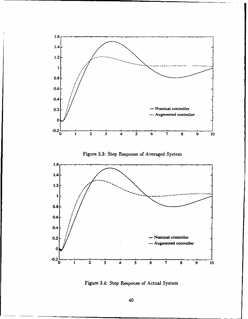
The resulting closed loop step response of the averaged system with the nominal controllerand the augmented controller KN(x) are shown in Figure 3.3.

The closed loop response of the original non-averaged system (3.1) with the nominal controllerK,... and the augmented controller (Ko,, Q) are shown in Figure 3.4. It can be seen that theactual and averaged closed loop step responses are almost identical which is in agreement withthe result of Theorem 3.3. Also, both the actual and averaged closed loop step responses withthe respective augmented controllers satisfy the design criteria.

5.3.5 DISTURBANCE REJECTION

The question of when the disturbance w can be completely decoupled by feedback controlfrom the regulated output z in the system (3.1) led to the development of geometric controltheory. The so-called disturbance decoupling problems for linear time-invariant systems havebeen investigated extensively in the last two decades. The problem is to find a compensator suchthat the closed loop transfer function from disturbance w to desired output z is equal to zero.

39

1.6

1.4

1.2

0.8,/-

0.6 :

0.4-

0.2-- Nominal controller

--- Augmented controller0

-0. 2 0 1 5, 6, 7 8 9' 10

Figure 3.3: Step Response of Averaged System

1.6

1.4-

1.2

0.8-

0.6

0.4

0.2-- Nominal controller

--- Augmented controller0

"0"2 1 2 3 4 5 6 7 8 9 10

Figure 3.4: Step Response of Actual System

40

Using the concept of (A, B)-invariance, the disturbance decoupling problem with state feedback(DPP) was solved in [77]. The problem of disturbance decoupling with state feedback and theextra requirement of internal stability (DPPS) was solved in [781, [79]. A detailed reference forthe above mentioned problems can be found in [80].

In this section, we study the disturbance decoupling problem with closed loop vibrationalcontrol. In particular, for the system (3.1) with Dz,, = 0, i.e.

i(t) = Ax(t) + Bu(t)f + Bw(t), (3.26)

z(t) = C"X(t),

we will establish conditions under which a state feedback of the form

u = K-x , (3.27)

can be found which decouples z from w. Similar to the approach in Section 5.3.3, we will firstderive the averaged equation for the closed loop system (3.26), (3.27). Let t(7) be a fundamentalmatrix for BKf(r) and introduce the substitution

ý(r) = 0(040•)

Then the corresponding averaged equation of the closed loop system (3.26), (3.27) is

t= 4-1 At +,t-1 B( w, (3.28)

Assume that (A, B) in (3.26) is controllable, then without loss of generality, let (A, B) be in

the controller canonical form:

0 1 ... 0 r0o

A = 0 0 ... 1], B= 0--an -- an-1 ... -a,

C,= Co c. c..

With state feedback

U= -x=- ikn ... k- ] k ,

the averaged closed loop system (3.28) reduces to

= (A- B7F) + B~w, (3.29)- CZ

where 7? is defined in (3.12).It follows from Theorem 3.3, that if the transfer function corresponding to

(A, B, C.) has relative degree > 2, the actual regulated output z will be arbitrarily close to

41

-'. Hence, our goal is to determine T for the averaged linear time-invariant system (3.29) so thatT is decoupled from w. This will in turn ensures that for the original non-averaged system (3.26).the regulated output z will also be decoupled from the disturbance w.

To solve the disturbance decoupling problem for the averaged system (3.29), we first introducethe following definition :

Definition 3.1: A subspace V C X = 1R' is said to be (A, B)-invariant (or controlled-invariant) if there exists K : X --, U such that (A - BK)V C V.

Theorem 3.4: [801 A subspace V C R' is controlled-invariant if and only if AV CV + ImB.

Corollary 3.1: Consider the system (3.29) with C # 0. Then V C kerC does not containthe vectore,,=[0 ... 0 1 iT.

Proof: We shall prove by contradiction. Let ej denotes the i - th standard basis vector.Assume that en E V. From Theorem 3.4, for vi = e,,, there exists a wi E V and ui E U = R suchthat

Ae,, = wi + Bui .

Hence wi = e,-i E V. Applying Theorem 3.3 again with vi = e,,- 1, we see that e,- 2 E V.Repeating this procedure, we see that ei,e 2,. . .,ee, E V. Hence dim(V) = n and we obtain acontradiction. Q.E.D.

Definition 3.2: The system (3.29) is said to be disturbance decoupled by closed loop vibra-tional control if there exists Kf of the form (3.12) such that

<A-B'KIImB. > C kerC,

where

< AjImB >'_- ImB + AIm.B +... + A n-1ImB.

Theorem 3.5: Assume that the transfer function corresponding to (A, B, C,) in system(3.29) has relative degree 2. Then the system (3.29) can be disturbance decoupled by closedloop vibrational control if and only if there exists a controlled-invariant subspace V satisfyingImB, C V C ker C.

Proof: The necessity is well known and established in [801. To prove sufficiency, we needto show that there exists a K E "K(V) = {I : X -+ UI(A - B(-K)V C V and V C ker C}satisfying (3.12). Let vj,... , v, be a basis for V. From Corollary 4.1, we know that e,, ý V. Nowen-1 V V since c,-. 2 # 0. Applying Theorem 3.4, for each vi,i = 1,...• , there exists a wi E Vand ui E U -R such that

Avi = wi + Bui ,

where B : U -- X. Let v,,+ 1,... , v,_ 2,e,,_ 1,e, be a set of vectors such thatvl,. .. ,V•,++ .... 1 2,Ve,2.-1 7 e,n is a basis for 1'n. Define 7K by the equation

F [vi ... V" Vu 1 . .]. Vn-2 cn- 1 e, = [u, ... Ul tp.1 ... tL- Un.1 Un] ,

where the scalars u•,+1,... ,u,,.- 2 are arbitrary and u.- 1 > 0 and u, = 0. Clearly, K satisfying(3.12) exists and is computable since the matrix [vi ... v,,v,,+1 , v,...2e,_.e,] is non-singular.Q.E.D.

It follows from Theorem 3.3, that if the averaged output i is decoupled from w, then theeffects of w will also be decoupled from the actual output z. The corresponding state feedbackgain K for the original non-averaged system (3.26) can be easily computed from (3.12).

42

5.4 PART 4. VERY HIGH HARMONIC CONTROL IN HELICOPTERS

5.4.1 INTRODUCTION

Helicopter vibration is a long standing problem. From the earliest days of rotorcraft develop-ment, oscillatory motions of the non-rotating portion of the airframe have been a matter of seriousconcern. Vibration affects adversely pilot performance and passenger comfort and increases oper-ation costs and maintenance requirements, limiting the use of helicopters in commercial aviationand military operations.

Traditionally, rotor induced vibration reduction efforts have focused on altering blade andfuselage dynamic characteristics or supplementing the rotorcraft with vibration isolators andattenuators. These passive methods have met with limited success [3]. Considerable researchhas been done on "active" techniques, which make direct use of vehicle control. One of the mostwidely used method of active control is the Higher Harmonic Control (HHC). HHC involvesdriving the blade pitch angle at the frequency N/rev (N is the number of blades) in orderto cancel the effect of vibratory airload transmitted to the fuselage. Recent experiments, [31-

o51, have shown that HHC may lead to an order of magnitude reduction in fuselage vibrations.or this method to be effective, not only the amplitude but also the phase of the oscillations

introduced should be chosen appropriately, depending on the flight conditions. The purpose ofthis research is to show that if the frequency of the oscillations introduced is much greater thanN/rev, the phase dependency disappears. To distinguish this approach from HHC, we call itVHHC, the Very High Harmonic Control. This part of the report presents a simple model and ahypothetical explanation of the efficacy of VHHC. The development presented here is based onthe ideas of vibrational control. Vibrational control is a method for changing dynamic propertiesof systems by introducing a control which enters the open loop dynamics as an amplitude ofa periodic, zero average function. The theory of this control technique has been developed inSection 5.1. As it has been pointed out in Section 5.1, vibrational control is a useful tool forachieving two conflicting control goals when only one actuator is available. This is exactly thecase in helicopters where the rotor blade pitch is used to accomplish both the desired aircraftaltitude and the fuselage oscillations suppression.

The application of closed loop vibrational control requires the knowledge of a dynamic modelof a system under consideration. Unfortunately, due to uncertainties associated with dynamics,measurement data and model structure, the mathematical modeling of helicopters for handlingqualities, performance, and flight control is a very difficult problem. The modeling of helicoptersis further complicated by numerous energy sources which cause fuselage vibrations. These en-ergy sources are (i) alternating aerodynamics forces acting on the rotors, (ii) engine vibrations,and (iii) aerodynamics forces acting on the fuselage and nonrotating parts of the machine. Therotor system, which transmits the vibratory airloads to the fuselage through the rotor shaft, isone of the most significant contributors to helicopter vibrations [23]. The rotating blades createvibratory airloads containing all harmonics of the rotor rotational frequency which are passedfrom the blades to the pylon and then to the cabin through complicated load paths. These loadsare felt as vibratory forces and moments whose frequencies are integer multiples of the bladepassage frequency (number of blades times rotational frequency). No simple models describingthese phenomena are available. Therefore, for the purposes of this research, we develop a sim-plified qualitative model of a helicopter and consider only the fixed airframe vibrations excitedby the rotor. Aerodynamic effects are faked as follows: Vibratory air load generated by therotating blades is modeled as a periodic function of the rotational frequency. The aerodynamicperturbations induced by the rotor on the fuselage are modeled also as a periodic function withfrequency equal to the blade passage frequency. Finally, incremental aerodynamic forces gener-ated by VHHC are modeled by another periodic function with high frequency. For simplicity, allthese functions are chosen as sinusoids, however this choice does not affect the qualitative resultsof this thesis.

Using this model, this thesis gives a phenomenological explanation of the efficiacy of VHHCin helicopter oscillations suppression. The outline of this section is as follows: In Section 5.4.2,a simple model of a helicopter is developed. Sections 5.4.3 and 5.4.4 are devoted to analysis of

43

F/2

F2x

Fy

Figure 4.1: Simple model of a helicopter

this model with and without VHHC in hover and forward flight, respectively. In Section 5.4.5,

the effects of wind gusts are examined.

5.4.2 QUALITATIVE MODEL

Consider a simple, qualitative model of a helicopter shown in Figure 4.1. The platform withmass m, and the pendulum with mass m2 are intended to model the rotor and the fuselage,respectively. The rotor generates the lift force, F, and induces aerodynamic perturbations, To,on the rotational degree of freedom of the fuselage. Force F and torque T# are modelled as

F = Fo+aosinwt, (4.1)To = #sinNtat,

where F0 is the steady lift due to the conventional rotor blade pitch control, ao sin wt is the peri-odic part of the lift due to vibratory airload, w is the rotor rotational frequency, N is the numberof rotor blades, ao and P are parameters that model the strength of the periodic components.

When VHHC is introduced, F is defined as follows:

F = Fo + ao sinwt + sin, 0 < 1. (4.2)

44

The small parameter f is intended to model the high frequency of VHHC. Although in generalthe amplitude of blade feathering is small (i.e. of the order c), the aerodynamic forces generatedby oscillating airfoils are proportional not only to the law of oscillations but also to the firstand second derivative of this law [831. Therefore, the amplitude of the VHHC generated forceis (4.2) is assumed to be 2. Note that the effect of differentiation, mentioned above, has beenobserved experimentally in [29] where higher HHC frequencies required smaller HHC amplitudesto suppress the fuselage vibrations.

The constant part of the lift, F0, is chosen to compensate for the system weight and toproduce a control force to ensure the desired helicopter altitude. Therefore, F0 is defined as

Fo = (Mi + m 2)g - kx (4.3)cos I4

where g is the acceleration of gravity, p is the rotor tilt angle and k is the gain of the altitudecontroller.

In addition to force F and torque T#, two more forces act on the system, F, and Fy. Theseare intended to model wind gusts and are assumed to be of an impulsive nature. A specific formof F, and Fy is described in Section 5.4.5.

Given the system of Figure 4.1 and forces (4.1), (4.2), we write the Lagrange equation for theplatform mi (rotor) and for the pendulum m 2 (fuselage) as follows:

(Min + M2) + m 21i sin0 + m 162 cosO + (Mi + m 2)g- Fcos tu - F. - (i , (4.4)

(Mi + m 2)j + m 2 eecosO - m 216 2 sinO= Fsinp - F1 - (ý , (4.5)

m 2t20 + m 21(i sin 0 + 9 cos 0) + m2 fg sin 0 = To + F., sin 0 + F.1 cos 0 - 76, (4.6)

where x, y and C denote the altitude, horizontal distance and dampling coefficient of the platformand 0, t and q the angle, length and damping coefficient of the pendulum.

The dynamics of this model are analyzed in Sections 5.4.3-5.4.5 using both a theoretical studyand numerical simulations. For simulation purposes, the parameters involved in (4.4)-(4.6) havebeen chosen as follows: m, = 0.01kg, M2 = 0.1kg, t = 1/v/Thim, ¢ = 0.6, 17 = 0.1, k=5, g=9.8m/sec2, CO =- = 0.1, N=3, w = 1 and e = 0.01.

5.4.3 ANALYSIS: HOVER

To model a helicopter in hover, we set p = 0. Assuming that F. = Fy = 0 and consideringonly the vertical and angular motions of the pendulum-platform system, we reduce equations(4.4)-(4.6) to the following form:

(MI + m 2)i + m 2ti sin 0 + m 2t62 cos 0 + (MI + m 2)g = F - (i , (4.7)

M2 02 + m21(i + g) sin 0 = To - ilO. (4.8)

The effect of VHHC in suppressing the vertical acceleration ; and the angular acceleration 6of the system (4.7), (4.8) is analyzed by considering three different cases. In the first case, thesystem is constrained to move only in the vertical direction (one degree of freedom), i.e. 0 =_ 0.In the second case, the system is analyzed with no constraint on its angular motion (two degreesof freedom) but without VHHC, i.e. a = 0. Finally, in the third case we investigate the systemperformance with VHHC, i.e. a # 0.5.4.3.1 One Degree of Freedom without VHHC

If we assume that the pendulum is fixed rigidly to the platform and therefore cannot executeangular motion, equations (4.7) and (4.8) reduce to the following single dynamical equation:

(in] + Mn)i + (Mi + •2 )g = FO + ao sinwt - (i . (4.9)

45

where

A, (4.16)V/(m2ig - m 2t

2 N 2W2 ) 2 + 772 N 2W2

S2.69,

anda, - tan-1 (m 2 g 7-rn 2wN2

Thus, the steady state angular acceleration is given by:

.,3(t) = -N 2w2 AA,#sin(Nwt + a,) (4.17)

Substituting (4.15) into (4.7), we obtain the steady state solution for the altitude of the platform:

x33(t) = MIcrosin(wt + •,) - (NwAl p) 2M2 m21cos(2(Nwt + a,) + Ql) , (4.18)

where

M2 = (4.19)/(k - (ml + m2 )4N 2w 2)2 + 4N 2w2ý2

- 0.267,

and

-- (-k - (MI + M 2)4N2W2 "

Thus, the steady state vertical acceleration of the system is:

i**(t) = -w 2M1 ao sin(wt + VI) + 4N 2w 2M 2m 2r(ApNw) 2 cos(2(Nwt + a,) + Ql) • (4.20)

A comparison of (4.20) with (4.12) shows that the two degrees of freedom system exhibitsvertical oscillations with both the rotational and the blade passage frequencies. The lattercomponent contributes significantly to the fuselage vibrations when the helicopter is in hover[85]. This leads to a conclusion that, in the two degrees of freedom system, the aerodynamicperturbations, To, generated by the rotor, excite the fuselage vibrations which then are passedon back to the rotor. This positive feedback is responsible for the large vertical acceleration ofthe system at hand.

This conclusion is supported by numerical simulations of (4.13), (4.14). Results are illustratedin Figures 4.3 and 4.4 (ct = 0), where equations (4.13), (4.14) are solved under zero initialconditions. These figures, which are in a good agreement wit estimates (4.15)-(4.20), show thataerodynamic perturbations, To, excite oscillations of the pendulum with a frequency equal to theblade passage frequency of 1.5/7r Hz. As a result, the pendulum has an angular acceleration ofthe same frequency and an amplitude of about 2.7 rad/s 2 as can be seen in Figure 4.4(b). Thedynamic excitation of the pendulum is subsequently passed on to the platform and generatesadditional vertical motion. Compared with Figure 4.2(a), Figure 4.3(a) shows that the altitudeof the platform is excited by both the 0.5/r Hz vibratory airload generated by the rotor and the3/r Hz vibration due to the oscillations of the pendulum. Thus, as shown in Figure 4.3(b), theresulting vertical acceleration of the platform also exhibits the effects of both the rotor vibratoryairload and the oscillations of the pendulum. This latter component accounts for the largevertical acceleration of about 0.2 mrs 2 , i.e., an order of magnitude increase in comparison withthe one degree of freedom system.

47

5.4.3.3 Two Degrees of Freedom with VHHCWith VHHC, the vertical and angular accelerations of the system can be obtained by substi-

tuting (4.2) into equations (4.7) and (4.8):

sin Nwt sin Oao sin wt + a-sin(!)) , (4.21)

M1 +M 2 2 M 2 2sin 20 + sin0m +M 2 - m 2 sin 0 2(m, + m 2) e(m, + m 2)

+ sin 0 - 1 sie(mn + m 2) t M2 mosin wt sin +

sin sin 0 + - in sNt (4.22)

I(mI + M 2 ) f n2

2 s

The terms in the right hand side of (4.21) and (4.22) contain the aerodynamic loads associatedwith the rotor vibratory airload, aerodynamic perturbations, and the VHHC. The VHHC term isof much higher frequency than the other two components. In practice, high frequency componentof the vertical acceleration is attenuated by passive damping in the cabin. It is therefore justifiableto consider only the filtered, or averaged with respect to high frequency, vertical and angularaccelerations of the system. This is the standard methodology of vibrational control [11]-113],where high frequency parametric oscillations are introduced in order to improve the averaged (orfiltered) behavior of the system. To obtain the averaged equations we first use the generatingequations technique of [201 that reduces (4.21), (4.22) to the standard Bogoliubov's form andthen use the averaging principle of [21], to derive the averaged equation. For the system at handthe resulting averaged equations are (see Appendix A2 for details)

1 (14 sin4'+m 2 gsin2q_M m+M2 -rn 2 sin 2 4'

(~ -a 2 sin• 2o 2)2 02)

-m~e 2P(ml + m 2 - m 2 sin

cos4'-kz-( i- .jsinNwtsin4'+aosinwt) (4.23)

- mi + M in in2 (M 2 (a ~2 sin 2 04 si 2 0)2S=MI + M2 - M2, sin GM 21r+'M2) (20(m, + m2 - M2 sin #)

2m 20(mi + M2 - m 2 sin2 4) sin 24kz sin 0 + (i sin 4--sin '- 17

+I(M) +M2) (M, +M2) 2

I(mi+m2 ) a0 sin wt sin 0 + I P sin Nwt (4.24)

where z and 4 denote the averaged altitude and angle, respectively.Comparing (4.21), (4.22) and (4.23), (4.24), we observe that the introduction of VHHC results

in additional terms containing amplitude a. To analyze the effects of these terms, we first reduce

48

(4.23), (4.24) to the form (4.7), (4.8). Then, since 0 is small, we negiect the first term containingQ' in (4.24) and approximate the denominator of the remaining term containing a' by m1 + mn 2 .Hence we write (4.23), (4.24) as:

(MIn + m2 ). + rnM2 sin P + M 2 fý2cos6 = a0 sin wt - kz - . (4.25)

m 2e'4) + m 2e + g + a2± C sins = sin Vwt - i7. (4.26)

Equation (4.25) is identical to (4.7) but unlike (4.8), equation (4.26) has an additional termcontaining a. Since the vertical acceleration - of the fuselage is generally of the order of 0.1g [84).for small 0 we can neglect the term m2f.• sin 4 and replace sin 0 by 0 and cos 0 by 1. Then thesteady state solution of (4.8) can be represented as

0.,(t) = A 2 3sin(Nwt + a2)

where

A21 222+722O (4.27)V(m 2tg + 2 - msg•N 2w2 )2 + i12Nsw2

S0.23, for a = 1,

and

02 = - tanif (M 24g + M(.+ 2- m 2 e2N2w2

A comparison of (4.27) with (4.16) shows that the VHHC term in (4.26) leads to an orderof magnitude reduction of the angular vibrations of the fuselage, i.e. to the stiffening of thesystem. As it follows from (4.20) (with A,, replaced by A2 and a, by 02), this results in anorder of magnitude reduction in the vertical acceleration of the system. Therefore, the effect ofVHHC can be interpreted as the decoupling of the positive feedback from the rotor through theaerodynamic perturbations to the fuselage and then back to the rotor.

This conclusion is supported by numerical investigation of (4.23), (4.24) (see Figures 4.3 and4.4 for a 9 0): Figure 4.4(a) shows that VHHC significantly reduces the oscillations in thependulum induced by the rotor vibratory airload. The resulting vibratory load suppression inthe angular acceleration is illustrated in Figure 4.4(b). The attenuation of the oscillations in thependulum produces a reduction in the dynamic load transferred back to the platform. As canbe seen in Figure 4.3(a), the 3/7r Hz vibrations generated by the oscillations in the pendulum onthe vertical motion are greatly attenuated. Note that this attenuation improves as the amplitudeof VHHC is increased (see Figure 4.5). For a = 1, the effect of these oscillations is virtuallyeliminated. In particular, the steady state vertical acceleration is about 0.02 m/s'. The 3/rHz vibration due to the oscillations in the pendulum has been eliminated and the remainingvibration in the vertical acceleration is at a frequency of 0.5/7r due to the rotor vibratory airloadaO sin wt. Thus, the introduction of VHHC forced the model to behave almost as a one degreeof freedom system.

5.4.4 ANALYSIS: FORWARD FLIGHT

To6 study the performance of a VHHC-equipped helicopter in forward flight, we considerequations (4.4)-(4.6) and assume that there is no wind gusts, i.e. F, = Fy = 0. Similar to Section5.4.3, we analyze the efficacy of VHHC in suppressing the vertical acceleration i, horizontalacceleration j and angular acceleration 0 by considering three different cases: (i) the system isconstrained to move only in the vertical and horizontal direction (two degrees of freedom), (ii) the

49

system has no constraints on its angular motion (three degrees of freedom) but without VHHC,i.e. a = 0, and (iii) the system with three degrees of freedom and with VHHC, i.e. n $ 0. \Veassume that the system's parameters are the same as those defined in Section 5.4.2 and choosep = 5 deg.5.4.4.1 Two Degrees of Freedom without VHHC

If the system (4.4)-(4.6), with F. = Fy = 0, cannot execute angular motion, then the system'sdynamics are governed by the following two equations:

(Ml + m 2 ): + (Mi + M2)g = (F0 + ao sin wt) cosp - , (4.28)

(MI + m2)h = (Fo + caosin wt)sinp -ý . (4.29)

Here again we observe the absence of the coupling terms due to angular motion. The response ofthe vertical and horizontal acceleration is affected only by Fo and a0 sin wt and no blade passagefrequency is involved. Numerical solutions of (4.28), (4.29) are illustrated in Figures 4.6 and 5.7for 0.155 m/sec initial horizontal velocity and all other initial conditions equal to zero. Fromthese figures we conclude that steady state vertical and horizontal accelerations are small (about0.02 m/s 2 and 0.002 m/s 2 respectively) and are of 0.5/7r Hz frequency due to the rotor vibratoryairload a0 sin wt.5.4.4.2 Three Degrees of Freedom without VHHC

Consider equations (4.4)-(4.6) with angular motion but without VHHC (i.e. a = 0). Thevertical, horizontal and angular accelerations can be expressed as:

M M2 0 M2tsinO -1.~M2 t6 G (MIn + M2)g + FCos p-0 mI +m 2 m 2 tcosO m2t92 sinO + F siny -

Sm 2tsine M2 1COSO M2 t 2 I -M2egSin0 + To - j•d

(4.30)

where F is given in (4.1). An approximate analysis of these equations can be carried outby using the method of Section 5.4.3.2. Here, however, we investigate the response of system(4.30) by performing simulation of these nonlinear equations with an initial horizontal velocityof 0.155 m/sec and all other initial conditions equal to zero. Similar to Figure 4.4(a), in Figure4.10(a) with a = 0 we observe that the aerodynamic perturbation To generates oscillations in thependulum with a frequency of 1.5/7r Hz. These oscillation are, in turn, transferred back to theplatform and produce additional motion in the vertical and horizontal directions. Thus, as shownin Figures 4.8(a) and 4.9(a), the resulting steady state altitude and horizontal velocity displaythe effects of both vibratory airload a0 sin wt and the oscillations of the pendulum. Again, thislatter component accounts for most of the vertical and horizontal accelerations.5.4.4.3 Three Degrees of Freedom with VHHC

With VHHC, the system's dynamic equations are governed by equations (4.30) with F de-fined in (4.2). As mentioned in Section 5.4.3.3, the high frequency component due to VHHCis filtered out by passive damping of the cabin, and hence it is of interest to consider the fil-tered vertical, horizontal and angular accelerations of the system. Using the generating equationmethod proposed in [20], we reduce (4.30) to the standard Bogoliubov form and apply averaginganalysis [21]. The averaged equations obtained are as follows (see Appendix A2 for details)

Im2(calpsin2#+sinpco&2#) mjjý-2c e= m2 sin 2 _ sin1[ m(m,+m,) m 2) 2m,tm,+m, 2 M1m2(com p sin 2#-uncoo 2#) , sin# mj+2-mga • C•.5Smt(-Im 1 1~ 2 t+M Z~;I mjt(rn+m3) m ml/

O(sin, 0 in #-co,/ o , 1" ,), -- Mn,_e.t

50

a (si fCOcsp +coo oin- L)

-m 2 e o2 + coso - k: + a0cospsinWt -

M2o2* (Z).. sin o + (m, +m 2 )gtanp -k.tanp+ aosin p sin.A -•p-mt9sin < + To -n+(

(4.31)

where z, v and 0 represent the averaged altitude, horizontal distance and angle respectively.The effects of VHHC when a helicopter is in forward flight and when a helicopter is in hover

are very similar: VHHC suppresses the oscillations of the pendulum induced by aerodynamicperturbations To; this, in turn, leads to a reduction of the dynamic load passed on back to thevertical and horizontal motions. This can be verified by performing the same analysis as in Section5.4.3.3. The effectiveness of VHHC in suppressing the vertical and horizontal accelerations whenthe helicopter is in forward flights is also illustrated by simulating nonlinear equation (4.31) withthe initial horizontal velocity of 0.155 m/sec and all other initial conditions equal to zero. Forclarity of illustrations, we present here the simulations only for a = 0.25 (other values of a arecharacterized in Figures 4.11 (a) and (b)). As it can be seen from Figures 4.8 and 4.9, the 3/7rHz vibrations in the vertical and horizontal motion are greatly attenuated. By comparing withFigures 4.6 and 4.7, we notice that VHHC stiffens the pendulum and forces the model to behaveas a 2 degrees of freedom system. We observe in Figure 4.10(a) that with VHHC the steady stateangular position of the pendulum is perpendicular to the platform. Since the angular position ofthe pendulum is initially at zero, this accounts for the large transient overshoots in Figures 4.8and 4.9.

5.4.5 EFFECTS OF WIND GUSTS

Next we analyze the effects of wind gusts on the performance of VHHC-equipped helicoptersduring forward flight. We introduce impulsive perturbations F. (at t = 1 sec and t = 4 sec)and FU, (at t = 2.5 sec and t Z 4 sec) into the system; the pulse duration and amplitude,respectively, are: 0.5 sec and 0.1 N. As it follows from Figures 4.12 and 4.13, VHHC still cancelsthe vibrations. However, since the gusts F. and Fy enter the system's equations directly in (4.4)and (4.5), VHHC is not very effective in suppressing their effects on the vertical and horizontalaccelerations of the system.

51

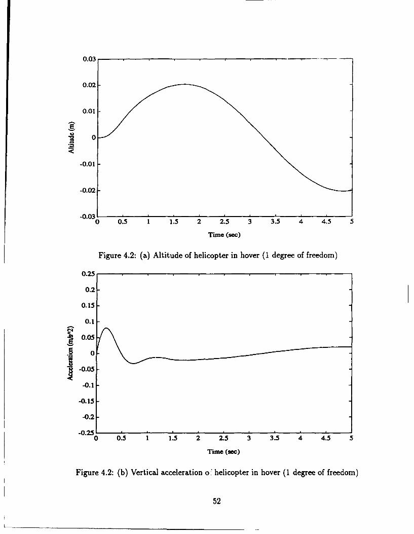
0.03

0.02

0.01

0

-0.01

-0.02-

0 0.5 1 1.5 2 2.5 3 3.5 4 4.5 5

Time (sec)

Figure 4.2: (a) Altitude of helicopter in hover (1 degree of freedom)

0.25

0.2

0.15

0.1

0 -. 05

-0.1

-0.15

-0.2-

0 0.5 1 1.5 2 2-5 3 3.5 4 4.5 5

Time (sec)

Figure 4.2: (b) Vertical acceleration o helicopter in hover (1 degree of freedom)

52

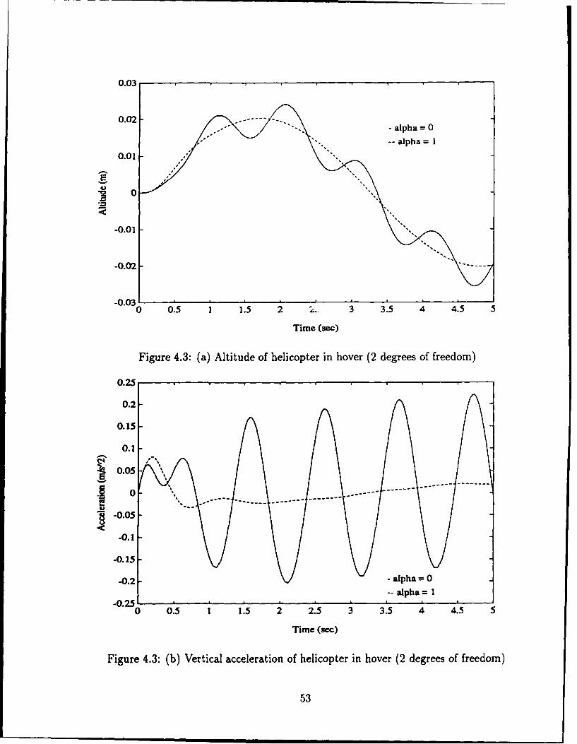
0.03

S- alpha =0

0.01

-0.01

-0.03'

-000 0.5 1 1.5 2 .. 3.5 4 4.5 5

Time (sec)

Figure 4.3: (a) Altitude of helicopter in hover (2 degrees of freedom)

0.25

0.2-

0.15

0.1-

0- ----- ---

0.05 - - a-- --. . . ..--- ----- ------ -- ---- - - - -

-0.05-

-0.1-

-0.15-

-0.2 - alpha = 0-- alpha= 1

-0.250 0.5 1 1.5 2 2.5 3 3.5 4 4.5 5

Time (sec)

Figure 4.3: (b) Vertical acceleration of helicopter in hover (2 degrees of freedom)

53

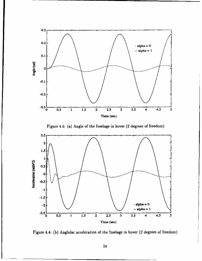
0.3

- alpha =0

-- alpha = 1

0.1

fto ---

-0.1

-0.2

-0.30 0.5 1 1.5 2 2.5 3 3.5 4 4.5 5

Time (sec)

Figure 4.4: (a) Angle of the fuselage in hover (2 degrees of freedom)

2.5

2

1.5 -

0.5

-1

-1.5-

-2 - alpha = 0

-- alpha 1-2.5

0 0.5 1 1.5 2 2.5 3 3.5 4 4.5 5

Time (sec)

Figure 4.4: (b) Anglular acceleration of the fuselage in hover (2 degrees of freedom)

54

0.2

0.18

0.16

0.14

0.12

.• 0.1

S0.08

0.06

0.04

0.02

0,0 0.1 0.2 0.3 0.4 0.5 0.6 0.7 0.8 0.9

Alpha

Figure 4.5: Vertical acceleration of helicopter in hover for different a

55

0.03

0.02-

0.01

. 0

-0.01

-0.02

-0.03 ' -0 0.5 1 1.5 2 2.5 3 3.5 4 4.5 5

Time (sec)

Figure 4.6: (a) Altitude of helicopter in flight (2 degrees of freedom)

0.4

0.3

0.2

0.1

S-0.2-

-0.3

-0.4-

-0.5

-0.6 '"','''0 0.5 1 1.5 2 2.5 3 3.5 4 4.5 5

Time (sec)

Figure 4.6: (b) Vertical acceleration of helicopter in flight (2 degrees of freedom)

56

0.5

0.45

0.4

0.35

S0.3 -

. 0.25

> 0.2

0.15

0.1

0.05

00 0.5 1 1.5 2 2.5 3 3.5 4 4.5 5

Time (sec)

Figure 4.7: (a) Horizontal velocity of helicopter in flight (2 degrees of freedom)

-1

-2

S-3

-4

-5

-6 1 I I I"0 0.5 1 1.5 2 2.5 3 3.5 4 4.5 5

Time (sec)

Figure 4.7: (b) Horizontal acceleration of helicopter in flight (2 degrees of freedom)

57

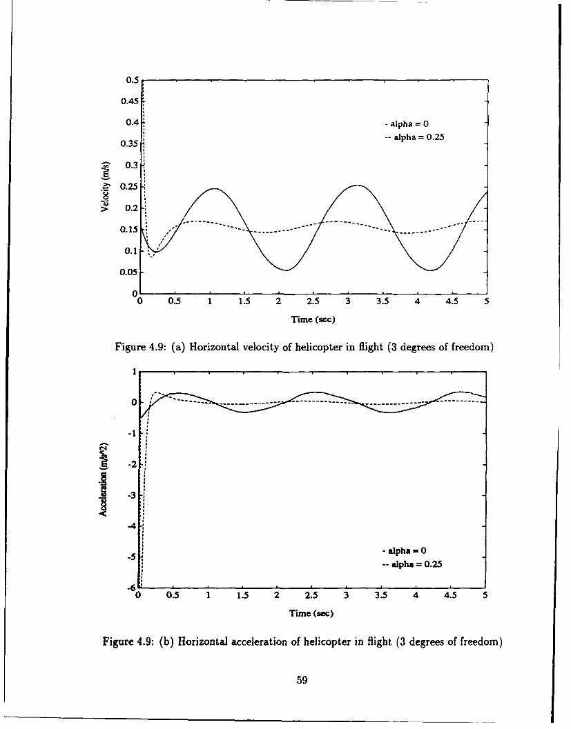
0.5

0.45

0.4 - alpha = 00.3 -- alpha =0.25

0.35

- 0.3

.•' 0.25

> 0.2

0.15 - ----- -

0.1

0.05

00 0.5 1 1.5 2 2.5 3 3.5 4 4.5 5

Time (sec)

Figure 4.9: (a) Horizontal velocity of helicopter in flight (3 degrees of freedom)

-alpha =0

j-5

-- alpha = 0.25

-60 0.5 1 1.5 2 2.5 3 3.5 4 4.5 5

Time (sec)

Figure 4.9: (b) Horizontal acceleration of helicopter in flight (3 degrees of freedom)

59

0.03

02- alpha = 0

02alpha 0.25

0.01

-0.01

-0.02-

-000 0.5 1 1.5 2 2.5 3 35 4 4.5 5

Time (sec)

Figure 4.8: (a) Altitude of helicopter in flight (3 degrees of freedom)

0.4

0.3

0.2

0.1 !C4'• -0.1

-0.2

-0.3

-0.4- alpha= 0

-0.5 -- alpha =0.25

0 0.5 1 1.5 2 2.5 3 3.5 4 4.5 5

Time (sec)

Figure 4.8: (b) Vertical acceleration of helicopter in flight (3 degrees of freedom)

58

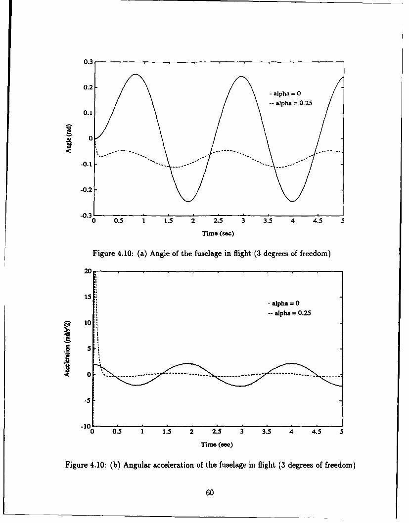
0.3

0.2--alpha= 0

-- alpha 0.25

0.1-

0

0.1

-0.2

-0.310 0.5 1 1.5 2 2.5 3 3.5 4 4.5 5

Time (sec)

Figure 4.10: (a) Angle of the fuselage in flight (3 degrees of freedom)

20

15 -alpha =0

-- alpha = 0.25

S 10:

S 5i

-5

-100 0.5 1 1.5 2 2.5 3 3.5 4 4.5 5

Time (sec)

Figure 4.10: (b) Angular acceleration of the fuselage in flight (3 degrees of freedom)

60

0.18

0.16

0.14

.- 0.12

0.1-

o0.08

< 0.06

0.04-

0.02

0I0 0.05 0.1 0.15 0.2 0.25 0.3 0.35 0.4 0.45 0.5

Alpha

Figure 4.11: (a) Vertical acceleration of helicopter in flight for different a

0.35

0.3

0.25

S0.2

"M 0.15

0.1

0.05

0 0.05 0.1 0.15 0.2 0.25 0.3 0.35 0.4 0.45 0.5

Alpha

Figure 4.11: (b) Horizontal acceleration of helicopter in flight for different a

61

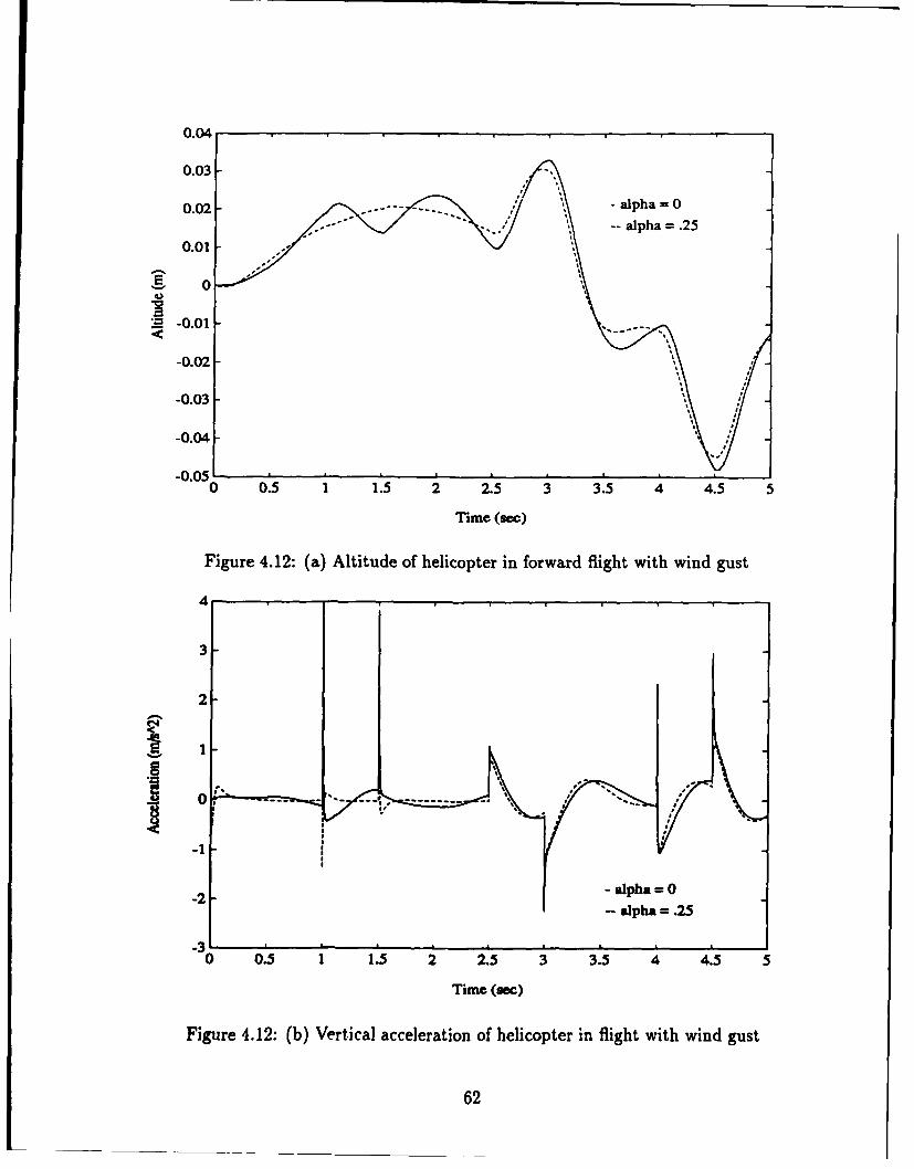
0.04

0.03

0.02- alpha 00.01 J° -- alpha =-.25

0.01

£ 0

":a -0.01

-0.02-0.03-\•

-0.*04

"000 0.5 1 1.5 2 2.5 3 3.5 4 4.5 5

Time (sec)

Figure 4.12: (a) Altitude of helicopter in forward flight with wind gust

4

3

2

0f -- -- ----- ------

-2l -alpha =0

- alpha = .25

"0 0.5 1 1.5 2 2.5 3 3.5 4 4.5 5

Time (sec)

Figure 4.12: (b) Vertical acceleration of helicopter in flight with wind gust

62

0.6

0.5

- alpha = 0

0.4 -- alpha =.25

0.34

0.2-:

0.1

0

-0.11"0 0.5 1 1.5 2 2.5 3 3.5 4 4.5 5

Time (sec)

Figure 4.13: (a) Horizontal velocity of helicopter in flight with wind gust

6

4

- alpha =0

2 -- alpha =0.25

0 " " - "- -- ---------

-2

-4

-6

"0 o.s 1 1.5 2 2.5 3 3.5 4 4.5 s

Time (sec)

Figure 4.13: (b) Horizontal acceleration of helicopter in flight with wind gust

63

5.5 PART 5. H2-OPTIMAL ZEROS

5.5.1 INTRODUCTION

Another important aspect in the control design of systems, besides ensuring sufficient numberof actuators as discussed in Section 5.1, is to determine the location of the control systemcomponents, namely actuators and sensors. In this part of the report, we treat this problem byconsidering a linear time-invariant SISO system of the form

i(t) = Ax(t) + Biu(t) + B 2w(t) , (5.1)y(t) = Cx(t) , x•E R", u, w,Y E JR.

In the design stage of the system (5.1), when no actuator positioning and disturbance protectionmeasures are yet finalized, input vectors B1 and B2 may be viewed as free parameters to be chosenso that appropriate performance specifications are satisfied. Among these, it seems reasonableto require that the transmission from the control u to the output y be maximized and thetransmission from the disturbance w to y be minimized. The term "transmission" could beformalized in a number of ways. We choose here a formalization in terms of transfer functions.Specifically, we say that the transmission from u to y is maximized if the H 2-norm of Ga,(s) :=C(sI - A)-1 B1 is maximized with respect to all Bi E Wr' such that 11B111 = 1 (11 "I denotesthe Euclidean norm of a vector). Similarly, the transmission from w to y is minimized (i.e. thedisturbance rejection is optimized) if the H 2-norm of G,,,(s) := C(sI - A)-`B 2 is minimized withrespect to all B2 E 1R' such that 1IB211 = 1. Since a choice of B, and B2 defines, for a givenA and C, the system's zeros, optimal B1 and B2 define the zeros, optimal with regard to theabove stated criteria. The purpose of this research is to give a solution to the H2-optimal zeroplacement problem for open and closed loop system (Sections 5.5.2 and 5.5.4) and characterizecontrol-theoretic properties of the resulting system (Section 5.5.3). In addition, we analyze therelationship between the open and closed loop H 2-optimal zeros (Section 5.5.5).

Since the L,, norm of y is often used for control system performance specifications, the H2-norm as a measure of optimality seems quite reasonable because it is induced by the L2 normon the input and the L,. norm on the output [86]. Other measures of optimality are, however,possible. For instance, Hughes and Skelton [87] optimize the controllability and observability"norms" to ensure good actuators and sensors configuration. Optimization of controllability,observability or the information matrix has been addressed in [39], [901, and [91]. An LQ-typeapproach is developed in [48]. In [38], actuator location has been addressed under a control effortsaturation assumption. The H2-optimization of this paper is related to the above cited literaturebecause sensor and actuator locations typically determine the matrices C and B1 respectively. Inthe present work, however, we assume that the directions of B1 and B2 can be chosen arbitrarilywhereas in practical applications components of vectors B1 and B2 might be functionally related.Accounting for these functional relationships will be a topic of future work.

5.5.2 H 2-OPTIMAL ZEROS IN OPEN LOOP ENVIRONMENT

5.5.2.1 Problem FormulationConsider an asymptotically stable SISO plant defined by a transfer function G(s) = C(sI -

A)-'B. Assume that vector B is subject to the constraint

BTMB=1 , (5.2)

where M is a symmetric, positive definite matrix.The problem of H2-optimal zero placement in open loop environment is formulated as follows:Find vector B, satisfying (5.2), such that IIGI2 is maximized (minimized).Remark 5.1: A natural choice for M in (5.2) seems to be M = I, resulting in IIBiI = 1. It

turns out, however, that this normalization may lead to a coordinate dependent optimal B and

64

consequently coordinate dependent zeros (see Section 5.5.3.3). If (C. A) is observable, a betterchoice is

Mf = CTC + ATCTCA +... + (A"' )TCTCA"-I

resulting in the normalization

(CB)2 + (CAB) 2 +... + (CA"- 1B) = 2 . (5.3)

Since CB, CAB,..., CA"- 1 B are the Markov parameters of G(s) and since

CA'B -d'g(t)'

CA'B = d ) =o,..,,,dt, It=o+'

whereg(t) =C-'{G()},

the normalization (5.3) constrains B to those that satisfy

S[d g(t) 2 . (5.4)

i= I t=0+

Thus, the optimal B is selected from all those that result in an impulse response which at t = 0'satisfy the normalization (5.4). This in fact defines a unit sphere in the space of impulse responsesof SISO, LTI systems of dynamic order at most n. It turns out that this normalization givesa coordinate independent optimal B and as a consequence, coordinate independent zeros (seeSection 5.5.3.3).5.5.2.2 Main Result

Theorem 5.1: Assume that A in (5.1) is Hurwitz and M in (5.2) is positive definiteand symmetric. Let L. be the observability Gramian, defined by ATLO + LoA + CTC = 0.

Then mnax JGuB1 ( min mIG,112) is attained at Bj* (B2 *) collinear with the eigenvector

of M-'L. corresponding to its largest (smallest) eigenvalue Amax(Amin). Under this choice

max JIG.II2 = Amax ( min IIG..II= Amin).BT•MBI=l (B2 MB2= 1Proof: First, note that M-1L. is a product of two symmetric, positive definite matrices

and so its eigenvalues are real and positive. Second, we observe that since JIGII2 = BTLOB (see[92]) and since (.)2 is a monotonic operation, the Lagrangian for the problem at hand is

L(B,7 , A) = 7 (BTLoB) - A(BT MB - 1),

where the multipliers -y, A E R are not simultaneously zero. The first order necessary conditionis [93]

VBL = -LOB- AMB = 0,

which yields7 M-1LoB = AB .

Since BTMB = 1,-f = 0 implies A = 0. Hence, it can be assumed without loss of generalitythat -y = 1. Furthermore, A > 0. Thus, any optimal B* should lie along the direction of aneigenvector of M- 1L. and

IIGI'll = B.TLOB" = AB°TMB* = A

65

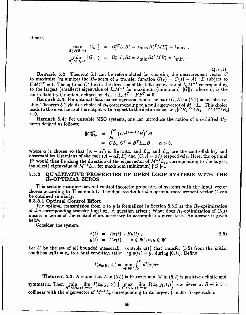
Hence,

max JIG.,,1' = BI LOB, = Ama•xB TrB = AmaxBMBI = 1

2

min IIG,,I2 = B TLoB; = AminB;2MB;= AminBTMB 2=i

Q.E.D.Remark 5.2: Theorem 5.1 can be reformulated for choosing the measurement vector C

to maximize (minimize) the H2-norm of a transfer function G(s) = C(sI - A)-1 B subject toCMCT = 1. The optimal C* lies in the direction of the left eigenvector of LCM-' correspondingto the largest (smallest) eigenvalue of LM-1 for maximum (minimum) uIG112 , where L, is thecontrollability Gramian, defined by AL, + LCAT + BBT = 0.

Remark 5.3: For optimal disturbance rejection, when the pair (C, A) in (5.1) is not observ-able, Theorem 5.1 yields a choice of B2 corresponding to a null eigenvector of M-iLo. This choiceleads to the invariance of the output with respect to the disturbance, i.e., (CB2 CAB 2 ... CA"-I B2 ]"-0.

Remark 5.4: For unstable SISO systems, one can introduce the notion of a a-shifted H2-norm defined as follows:

IG11IL = f (Ce(A-')*B) 2 dt= CLwCT=BTLo•B, a>0,

where a is chosen so that (A - a1) is Hurwitz, and L,, and L,,, are the controllability andobservability Gramians of the pair (A - a1, B) and (C, A - aI) respectively. Here, the optimalB* would then lie along the direction of the eigenvector of M- L.,, corresponding to the largest(smallest) eigenvalue of M- 1 Lo. for maximum (minimum) I JGJ12a.

5.5.3 QUXLITATIVE PROPERTIES OF OPEN LOOP SYSTEMS WITH THEH 2-OPTIMAL ZEROS

This section examines several control-theoretic properties of systems with the input vectorchosen according to Theorem 5.1. The dual results for the optimal measurement vector C canbe obtained similarly.5.5.3.1 Optimal Control Effort

The optimal transmission from u to y is formalized in Section 5.5.2 as the H2-optimizationof the corresponding transfer function. A question arises : What does H 2-optimization of G(s)means in terms of the control effort necessary to accomplish a given task. An answer is givenbelow.

Consider the system,

i(t) = Az(t) + Bu(t) , (5.5)y(t) = CX(t). XE WR",u,y E IR

Let U be the set of all bounded measurabi -ontrols u(t) that transfer (5.5) from the initialcondition z(0) = xo to a final condition satis ig y(ti) = yi during [0, t1 ]. Define

J(xo, y1 ,ti) = mrin j1 u2(r)drU(t)C-U fo

Theorem 5.2: Assume that A in (5.5) is Hurwitz and M in (5.2) is positive definite and

symmetric. Then min lim J(xo, y,,ti) (max lim J(xo, y,,t,1 ) is achieved at B which isBTMB=1 t3-o0 \B T MB-I ti-..oo /

collinear with the eigenvector of M-1 Lo corresponding to its largest (smallest) eigenvalue.

66

Proof: First we prove that

J(xo, Yi ,ti) (y, - Ce 4 (5 xo)6o , t , CeA(ti-r)BBTeAr(tj--)CTdr (5.6)

Indeed, a control u0 (t) that transfers (5.5) from the initial condition x(O) = xo to a finalcondition satisfying y(tl) = yj over [O,tl] can be calculated as follows:

u°(t) = BTeAT(tl-t)CTW-1(O, t1 )[y -_ CeAtIxo], t E [0, t], (5.7)

whereW(O, ti) = CeA(t1-,?)BBTeAr(t1-r)CTdr

.

This control is optimal in the sense that if ul(t) is any other control in U, then

f (ul~tj))2 > jt l (uO~t)) 2 dt .(5.8)

To prove this we note that

Y1 - CeAt'Xo ceAl-j-r)Bu°(r)d= CeA(t,-')Bul(r)d•

Therefore,

fo CeA(t2-)B(u'(T) - u°(T))dr = 0

Then

W- 1 (o, t) [y, - Ce I fo] jo CeA(i1-)B(ul(r) - u°(T))dr = 0

which is equivalent to

f"tl (UI(r) - UO(T)) (CeA(t--)B) T W-1 (0, tl) [Y, - CeAtlxo] dT = 0

From the last expression and (5.7), we obtain

0o (U'(7) - uo()) uO(r)d7 = 0

Therefore,

IO" (ul(r))2 dr = ot l ( r(T)- uo(r)+ uo(r)) 2 d

= t J U'(7) --)Uo(7)) 2d 2 d-+ (uo(r)) ,dT

+2j (ul(r) - uO(r)) Uo(r)d,

J U' ( 7-() -Uo(T)) 2 dr+ +I" (uo(T))• 2 •dr

which results in (5.8).

67

Thus, it follows from (5.8) that the minimum energy required to transfer the system (5.5)from x(O) = xo to a final condition satisfying y(tj) = y, is indeed given by (5.6). tlence if .4 isHurwitz, 2

lim J(Xo,y'1 , ti) -- (5.9)"t-00 T ýBT L o5J "

Since BTLoB, subject to the constraint BTMB = 1, achieves its maximum (minimum) at Bcollinear with the maximum (minimum) eigenvalue of M-'Lo, Theorem 5.2 is proved. Q.E.D.

Theorem 5.2 offers an alternative characterization of H 2-optimal transmission: The optimalB1 (B;) ensures minimum control (maximum disturbance) energy in transferring the systemstate from an arbitrary initial state to a final state, consistent with the specified output, over anasymptotically infinite time interval.5.5.3.2 Controllability Properties

As stated in Theorem 5.1, system (5.1) with B1=B1 * has H2-optimal (maximal) transmissionproperties from u to y. A question arises: Is there always at least some transmission from u toevery component of x in such a system? An answer is given below.

Theorem 5.3: Assume A in (5.1) is Hurwitz, M in (5.2) is positive definite and symmetricand the maximum eigenvalue of the matrix M-1L0 , where Lo is the observability Gramian of(5.1), is simple. Then system (5.1) with B1=Bl* and B2 = 0 is controllable if and only if thereexists no left eigenvector of A orthogonal to the eigenvector of M-1 Lo corresponding to its largesteigenvalue.

Proof: Follows directly from Theorem 5.1 and the PBH controllability test [94]. Q.E.D.Theorem 5.4: Assume A in (5.1) is Hurwitz and BI=B1 *, B 2 = 0. Assume further that

M = I, the observability Gramian Lo has distinct eigenvalues and rank [rn&-L.%] = n. Then

system (5.1) is controllable only if (Lo, LoAT - ATLo) is observable.

Proof: The theorem is proved by contradiction. Suppose B1 = Bj' and B2 = 0. If(Lo, LoAT - ATLo) is unobservable, then for some A, there exists x :A 0 such that

LoAT_- A TLo X = 0

i.e. L 0ATX = AATx, 7 #Amax•Since A is a simple eigenvalue of L. with a unique eigenvector x, this implies that ATX mustbe collinear with x, i.e. there must exist p such that ATx = px. This shows that XT is a lefteigenvector of A. Since both, x and Bl*, are eigenvectors of Lo,

xT B; = 0,

XT A = pXT.

Therefore, according to the PBH test, system (5.1) with BI=Bl* and B2 = 0 is uncontrollable[95]. Q.E.D.5.5.3.3 Coordinate Independence

Theorem 5.1 may yield optimal B1 and B2 which result in coordinate dependent zeros. Thefollowing statement gives condition on M which ensures coordinate independence.

Theorem 5.5: Assume that A in (5.1) is Hurwitz and M in (5.2) is positive definite andsymmetric. Let S be a similarity transformation and M be the representation of M in the newbasis. Then system (5.1) with BI=B,; and B 2=B2 yields zeros which are independent of thecoordinate transformation S if M - STMS.

Proof: From Theorem 5.1, B,* and B, satisfy

M-'LoBr = AmaxB•,

M-'LoB; = AminB;.

68

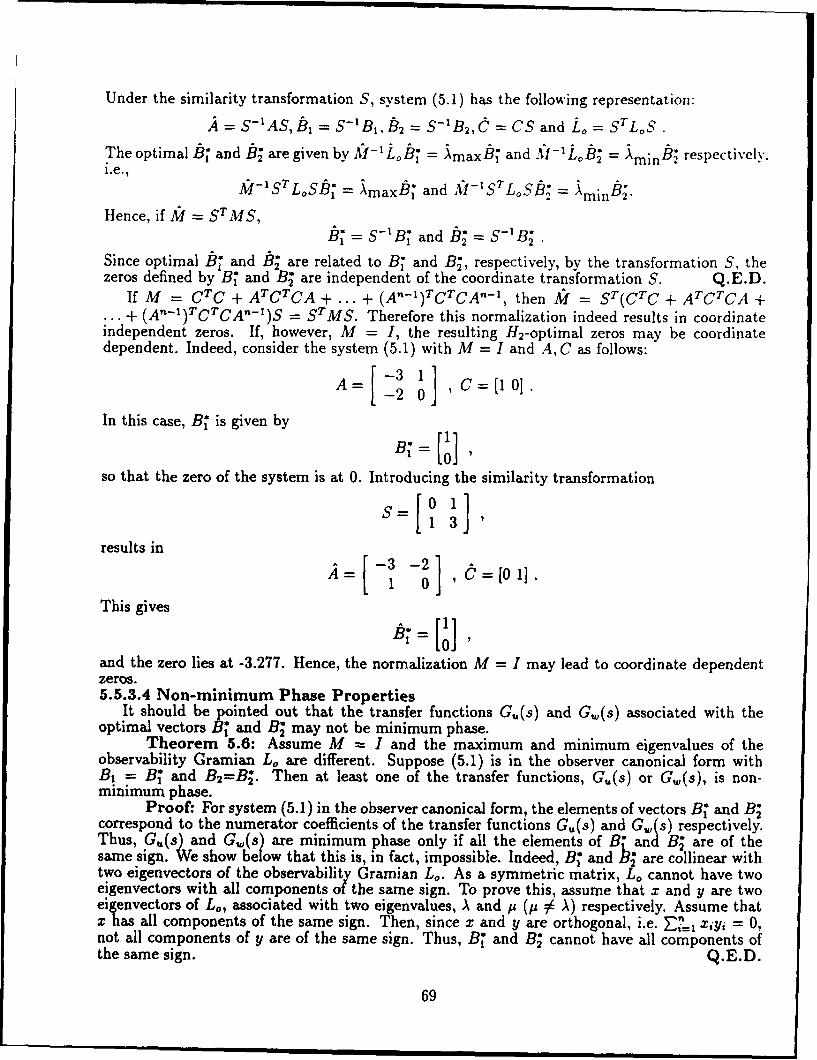
Under the similarity transformation S, system (5.1) has the following representation:

A = S-AS, B1 = S-'B1 , i32 = S-B 2 , C = CS and L" = STLoS .

The optimal b,[ and f are given by if Lo!B[ = Amax!bl and -l B = Ab; nh; respectively2 minB epcieyi.e.,

Mk-STLoS B = AmaxB[ and MI-STLoSB = Aminb;.

Hence, if Af!= STMS,

b; = S-'B; andf; = S-BB.

Since optimal B* and B; are related to B" and B;, respectively, by the transformation S, thezeros defined by B• and B; are independent of the coordinate transformation S. Q.E.D.

If M = CTC + ATCTCA + ... + (A?-1)TCTCAn-, then M = ST(CTC + ATCTCA +•.. + (A'-1)TCTCAn-1)S = STMS. Therefore this normalization indeed results in coordinateindependent zeros. If, however, M = I, the resulting H2-optimal zeros may be coordinatedependent. Indeed, consider the system (5.1) with M = I and A, C as follows:

A=[-3 1] C= [1 01-2 0

In this case, B,* is given by

so that the zero of the system is at 0. Introducing the similarity transformation

S= 1 3 '

results in

-1 0 "

This gives

and the zero lies at -3.277. Hence, the normalization M = I may lead to coordinate dependentzeros.5.5.3.4 Non-minimum Phase Properties

It should be pointed out that the transfer functions Ge(s) and G.(s) associated with theoptimal vectors Bj* and B, may not be minimum phase.

Theorem 5.6: Assume M = I and the maximum and minimum eigenvalues of theobservability Gramian Lo are different. Suppose (5.1) is in the observer canonical form withB, = B[ and B2=B2. Then at least one of the transfer functions, G,,(s) or G,,,(s), is non-minimum phase.

Proof: For system (5.1) in the observer canonical form, the elements of vectors B• and BOcorrespond to the numerator coefficients of the transfer functions G,,(s) and G,,,(s) respectively.Thus, G,,(s) and G,(s) are minimum phase only if all the elements of B* and B* are of thesame sign. We show below that this is, in fact, impossible. Indeed, B1 and h2 are collinear withtwo eigenvectors of the observability Gramian L. As a symmetric matrix, Lo cannot have twoeigenvectors with all components of the same sign. To prove this, assume that x and y are twoeigenvectors of L0 , associated with two eigenvalues, A and p (p #6 A) respectively. Assume thatx has all components of the same sign. Then, since x and y are orthogonal, i.e. ' xjyj = 0,not all components of y are of the same sign. Thus, B,* and B2 cannot have all components ofthe same sign. Q.E.D.

69

5.5.4 H 2-OPTIMAL ZEROS IN CLOSED LOOP ENVIRONMENT

5.5.4.1 Problem FormulationIn the closed loop environment, a number of problems concerning H2-optimal zeros can be

formulated. The following three are of importance in various control-theoretic situations:5.5.4.1.1 H 2-optimal zeros in the disturbance rejection problem

Here the system (5.1) is considered in a closed loop form, for instance, with u = Kx. DefineG(s) = C(sI - A - BIK)B 2 and we want to choose B2 such that JIGI12 is minimized subject toJIB 211 = 1 (or BTMB 2 = 1, M = MT,M > 0). Obviously, if (A+ BIK) is Hurwitz, the answer tothis question follows from Section 5.5.2 above: The optimal B2 is collinear with the eigenvectorof the closed loop observability Gramian, Lc', corresponding to its smallest eigenvalue. Here Lc'is defined by

(A + B1 K)TLcl + Lc'(A + B 1K) + CTC = 0.

Due to the separation property, the same result holds not only for state feedback, but also forobserver-based output feedback.5.5.4.1.2 H2-optimal zeros in the regulator problem

Consider the system

x = Ax+Bu, (5.10)y = Cx, xERB',u,yElR

E{xo} = 0, E{xoxT} =Q,

where xo = x(0). Assume that u = Kx, (5.11)

where K is chosen so that

J = E fjf (XCTI + u2) dt} (5.12)

is minimized. If (A, B) is stabilizable, (C1 , A) is detectable, it is well known that the optimal Kis given by

K == -BTp, (5.13)

where P is the positive semi-definite solution of

ATp + PA - PBBTP + C"TC1 = 0. (5.14)

The optimal value attained by functional (5.12) with feedback (5.13) is:

J* = Tr(PQ) . (5.15)

Obviously, the value J* may be further improved by minimizing J* over all admissible vectorsB. To cast this problem in H 2-norm minimization form, we define Q = BIBT and rewrite (5.14)as

(A - BBT P/ 2 )Tp + P(A - BBT P/2) + CTC1 = 0 . (5.16)

HenceJ* = Tr(PBIBT) = Tr(BIPB[), (5.17)

and from (5.16) and (5.17), the functional J* is equivalent to the square of the H 2-norm of thefollowing transfer function

Gi(s) = C 1(sI - A - BK/2)'BI • (5.18)

70

It should be noted that the matrix (A + BK/2) is Hurwitz due to the fact that LQ designs havea guaranteed gain margin from 1/2 to +oc [96]. Also, for a given A. B1 and C1, the choice of B.which determines K, will generally affect both the zeros and poles of the transfer function Gj(s)(see Example 5.2).

Thus, the problem of H2-optimal zero placement regulator problem can be stated as follows:Given (5.10), (5.11), (5.13) and (5.14), find vector B satisfying the constraint IIBII = 1 (or

BTMB = I, M = M', M > 0) such that IUGJ 112 is minimized.A necessary condition for the solution of this problem is given in Section 5.5.4.2.

5.5.4.1.3 H2-optimal zeros in the servomechanism problemConsider again system (5.10) and assume that

u = Kx + v , (5.19)

where v is an exogenous signal. The control gain K is assumed to be chosen according to thedesigner's favorite methodology, such as pole placement, LQG, HI, design, or any other. Theproblem of H 2-optimal zero placement in the servomechanism problem is formulated as follows:

Given (5.10) and a design methodology for K, find B satisfying IIBII = 1 (or BTMB = 1,M = MT, M > 0) which maximizes IIGv112 where

G,(s) = C(sI - A - BK)-'B . (5.20)

A solution to this problem is given below under the assumption that K is designed using theLQR approach, i.e.,

K = -BTp,

ATP + PA - PBBTP + CTC1 = 0.Remark 5.5: As it follows from (5.18) and (5.20), the main difference between the open and

closed loop H 2-optimal zero placement is in the fact that in the latter case, vector B affects notonly the zeros but also the poles of the transfer function.

Remark 5.6: The problems formulated above can be extended to dynamic output feedbackas well. Indeed, assume that we use a controller

u = Ki+v, (5.21)

x = A,+Bu+L(y-Ci). (5.22)

Then, it is well known that the closed loop transfer function from v to y is also given by (5.20).5.5.4.2 Main Result5.5.4.2.1 H 2-optimal zeros in the regulator problem

Theorem 5.7: Consider the closed loop system (5.10 ), 5.11), (5.13) and (5.14). Assumethat (A, B, C1 ) is stabilizable and detectable. Then min fjG3( 2 is attained at vector B only if

IOBIk=1it is collinear with an eigenvector of matrix S = PGP, i.e.,

(PGP - AI)B = 0, (5.23)

where P, G E RW'", are defined by

(A - BBTP)TP + P(A - BBTP) + PBBTp + C1cI =0, (5.24)

(A- BBTP)G+G(A- BBTp)T + B 1BT =0. (5.25)

In addition,IlGjIIl = A+ CGC[.

71

Proof: The Lagrangian for the problem is

L(B,P,G,-, A) = 7BTPBI + Tr(G[ATp + PA - PBBTp + CTC 1I]) + A(BTB - 1),

where -1, A E 1R and G E R"', G = GT, are the Lagrange multipliers which are not simultaneously zero. The first order necessary conditions for an extremum are as follows:

=L =7BiBT +AG+GAT - GPBBT BBPT pG=O,OPI8L-9 = -2PGPB+2AB=O.OB

Since A - BBTP is stable with (Cl, A) detectable, -y = 0 implies A = 0, G = 0 in the aboveequations. Hence, it can be assumed without loss of generality that -y = 1. Furthermore, G isnonnegative definite.

Equations (5.23) and (5.25) are thus obtained and (5.24) is equivalent to (5.14). From (5.25),we have

Tr(PBBT) = -Tr(P[A - BBTPIG) - Tr(PG[A - BBTp]T)"- -2Tr(P[A - BBT P]G)

= -2Tr(PAG) + 2Tr(PBBT PG)

= -2Tr(PAG) + 2BTPGPB.

From (5.23), (5.24) and knowing BTB = 1, we have

IIGjII = Tr(PBIB T)= -2Tr(PAG) + 2A

= -A+CGCIT+2A

= A+CIGCT *

Q.E.D.5.5.4.2.2 H2-optimal zeros in the servomechanism problem

Theorem 5.8: Consider the closed loop system (5.10),,(5.19), (5.13) and (5.14). Assumethat (A, B, C1 ) is stabilizable and detectable. Then max IIGII is attained at vector B only if

it is collinear with an eigenvector of matrix S = Lei - PGP - 2PLILo', i.e.,

(Lc'- PGP - 2PL Lo' - AI)B = 0, (5.26)

where P, L"', G and Lc' E WR"" are defined by the following equations:

(A - BBTP)TP + P(A - BBTP) + PBBTP + CITC , = 0, (5.27)(A - BBTP)TLI + L'(A - BBTp) + CTC - 0, (5.28)

(A - BBTp)G + G(A - BBTP)T - LiLc'BB T - BBTLeLLtL 0, (5.29)(A - BBTP)Lcc + Ld(A - BBTp)T + BBT = 0. (5.30)

In addition,max IIG II1 = CL ICT .

72

Proof: By forming the Lagrangian.

L(B, L., P, G, Lc', y, A) = -yBT LcB + Tr(G[AT P + PA - PBBTP + CTC1]-Lc'[(.4 - BBTP)TLcI+ Lc'(A - BBTp) + CTC]) -

A(BTB-1),

where Y, A E iR and G = GT, Lc' = (Lc')' are the Lagrange multipliers which are not simul-taneously zero. The closed loop observability Gramian Lc1 is defined by (5.28). The followingconditions are necessary for an extremum:

= AG + GAT - GPBBT - BBTPG - Lc'Lc'BBr - BBrLcILci =0

(5.31)

OL = (A - BBTP)LcI + Lc'(A - BBTP)T + 7BBT = 0, (5.32)

OL 2LoB 2PP -OL = 2-tLcB - 2PGPB - 4PLc Lc'B - 2AB = 0 (5.33)

Since A - BBTp is stable with (Cl, A) detectable, -y = 0 implies Lc' - G 0 and A = 0 in(5.32), (5.31) and (5.33) respectively. Hence, it can be assumed without loss of generality that-Y = 1. Furthermore, Le is nonnegative definite.

Equations (5.26), (5.29)-(5.30) are thus obtained and (5.27) is equivalent to (5.14). From(5.28) and (5.30) , we have

Tr(BBT Lc) = -2Tr(ALcLc) + 2Tr(LcPBBT L L)

= Tr(Lc'CT C) = CLeICT.

Q.E.D.Remark 5.7: Since equations (5.23)-(5.25) and (5.26)-(5.30) are all coupled, they are

formidable, indeed. Their relative utility may be justified by the following two arguments. First,these equations can be used to verify whether vector B optimal for an open loop system remainsoptimal ;-i the closed loop environment. Section 5.5.5 below examines this relationship. Sec-ondly, ite, ative procedures can be suggested for solving these equations (see below). Althoughthe convergence conditions for these procedures are presently unknown, it is easy to show thatthey always generate sequences which contain convergent subsequences. Indeed, since the opti-mization is performed over the compact set (B : BTB = 1), any sequence contains at least oneconvergent subsequence [97].

The following iterative procedure was tested on several examples for solving equations (5.26)-(5.30):

1) Choose a vector B(n), for n = 0 such that BT(n)B(n) = 1 (e.g. B(n) = [1 0 0 ... 0]T).

2) Solve the algebraic Ricatti equation (5.27) for n = 0 giving P(n).

3) Solve the Lyapunov equations (5.28) and (5.30) for n = 0 giving Lc'(n) and Lc'(n).

4) Solve the Lyapunov equation (5.29) for n = 0 giving G(n).

73

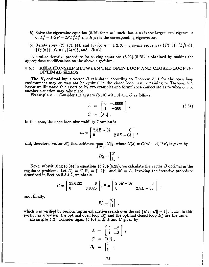
5) Solve the eigenvalue equation (5.26) for n = 1 such that A(n) is the largest real eigenvalueof L•' - PGP - 2PL•'Lc' and B(n) is the corresponding eigenvector.

6) Iterate steps (2), (3), (4), and (5) for n = 1,2,3,..., giving sequences {P(n)), {L'ý(n)),{Lc'(n)}, {G(n)}, {A(n)}, and {B(n)}.

A similar iterative procedure for solving equations (5.23)-(5.25) is obtained by making theappropriate modifications on the above algorithm.

5.5.5 RELATIONSHIP BETWEEN THE OPEN LOOP AND CLOSED LOOP H2-OPTIMAL ZEROS

The H 2-optimal input vector B calculated according to Theorem 5 .1 for the open loopenvironment may or may not be optimal in the closed loop case pertaining to Theorem 5.7.Below we illustrate this assertion by two examples and formulate a conjecture as to when one oranother situation may take place.

Example 5.1: Consider the system (5.10) with A and C as follows:

A - [ -10000 (5.34)

C [01].

In this case, the open loop observability Gramian is

L 0= [ E 2.5E-03 '

and, therefore, vector Bo1 that achieves max uG112, where G(s) = C(sI - A)-1 B, is given byIlBJI=1

Next, substituting (5.34) in equations (5.23)-(5.25), we calculate the vector B optimal in theregulator problem. Let C1 = C, B1 = [1 1]T, and M = I. Invoking the iterative proceduredescribed in Section 5.5.4.2, we obtain

G [25.0122 0 ] [P 2.5E- 07 0]G=0 0.025 ' =0 2.5E -03 '

and, finally,

which was verified by performing an exhaustive search over the set {B: IIBBI = I}. Thus, in thisparticular situation, the optimalopen loop B.* and the optimal closed loop Bct are the same.

Example 5.2: Consider again (5.10) with A and C given by

A 0 [ -2fl11 -3

C = [01],

74

and Ci = C, M I. The open loop optimal B., for this case turns out to be

whereas the regulator problem results in

Bc,= 04384].1 = 0.8988]

K = [0.0347 0.1465]

Obviously, the two vectors B.* and Bci differ significantly. Note also that the zero of the triple(A, B1 ,C1 ) is at -1 while that of the triple (A + B1tK/2, BI,CI) lies at -0.984.

Based on our experience in computing the optimal input vector B in open loop (Theorem5.1) and closed loop (Theorem 5.7), we are led to the following conjecture.

Conjecture 5.1: When the LQR methodology is used to compute the feedback gain K inthe closed loop case, optimal vectors Bot and Bt are close to each other for system with "fast"open-loop poles.

The reason behind such a conjecture is that for systems possessing open loop poles in the farleft half complex plane, the location of the closed loop poles will not be significantly differentfrom that of the open loop poles with a LQR controller. Hence optimal vector Bl obtained fromthe open loop system dynamics will be close to that of Bit.

However, in general, in a closed loop system with a specified feedback co-' -oller, for maximumH2-norm transmission from an exogeneous input to the output y, the choic,,. of the optimal inputvector must take into, onsideration the dynamics of the closed-loop system and not the open-loopdynamics. To be more precise, the choice of the input vector B and the controller design shouldbe performed simultaneously as presented in Theorems 5.7 and 5.8.

75

6 LIST OF PUBLICATIONS AND TECHNICAL REPORTS

3 1] P.T. Kabamba, S.M. Meerkov, and E.-K. Poh, "H2-Optimal Zeros," Proceedings of the30thConf. on Decision and Control. Brighton, U.K., pp. 2289-2290. Dec. 1991. An extendedversion of this paper ha&- been accepLed for publication i IEiLEE Tranzsactiorns o-, .tutornat:cControl. The full paper is in Univ. of Michigan Conir. Grp Report, CGR-92-16, Aug. 1992.

121 P.T. Kabamba, S.M. Meerkov, and E.-K. Poh, "Closed Loop Vibrational Control:Stateand Output Feedback Stabilizability," Proceedings of the 30th Conf. on Decision and Control,Brighton, U.K., pp. 2375-2376, Dec. 1991.

[3] P.T. Kabamba, S.M. Meerkov, and E.-K. Poh, "Closed Loop Vibrational Control:State andOutput Feedback Stabilizability and Pole Placement Capabilities," Univ. of Michigan Contr.Grp Repor,. 2GR-92-17, Aug. 1992. An extended version of this paper was submitted forpublication in IEEE Transactions on Automatic Control.

[4] P.T. Kabamba, S.M. Meerkov, and E.-K. Poh, "VHHC in Helicopters," Proc. AmericanControl Conference, San Francisco, CA, June 1993. An extended version of this paper wassubmitted for publication in Journal of Guidance, Control and Dynamics. The full paper is inUniv. of Michigan Contr. Grp Report, CGR-93-11, July 1993.

(5] P.T. Kabamba, S.M. Meerkov, and E.-K. Poh, "Stability Robustness in Closed LoopVibrational Control," Univ. of Michigan Contr. Grp Report, CGR-93-4, Feb. 1993. An extendedabstract of this report was submitted for publication in IEEE Transactions on Automatic Controland the 32nd Conf. on Decision and Control, San Antonio, TX, Dec. 1993.

[6] P.T. Kabamba, S.M. Meerkov, and E.-K. Poh, "Youla Parametrization in Closed LoopVibrational Control," Univ. of Michigan Contr. Grp Report, CGR-93-6, Feb. 1993. An extendedabstract of this report has been accepted for publication in IEEE Transactions on AutomaticControl. The paper has also been submitted for the 32nd Conf. on Decision and Control, SanAntonio, TX, Dec. 1993.

76

7 LIST OF PARTICIPATING SCIENTIFIC PERSONNEL

1. Semyon M. Meerkov, P.I., Professor.

2. Pierrc T. Kabamba, Co-P.I., Associate Professor.

3. Eng-Kee Poh, Research Assistant, Ph.D. Candidate, Expected Graduation Date July 1993.

-7I

8 BIBLIOGRAPHY

References[1] J. Shaw, "Higher Harmonic Blade Pitch Feathering for Helicopter Vibration Control," Sc.D.

Thesis, Dept of Aeronautics and Astronautics, M.I.T., Jan. 1980.

[2] W. Johnson, "Self Tuning Regulators for Multicyclic Control of Helicopter Vibration,"NASA TP-1996, 1992.

[3] E.R. Wood, R.W. Powers, J.H. Cline, and C.E. Hammond, "On Developing and FlightTesting Higher Harmonic Control Systems," Journal of the American Helicopter Society,Vol. 30, No. 1, pp. 3-10, Jan. 1985.

[4] G. Lehmann, "The Effect of Higher Harmonic Control (HHC) on the Four-Bladed HingelessModel Rotor," Vertica, Vol. 9, No. 3, pp. 273-284, 1985.

[5] F.K. Straub and E.V. Byrns, Jr., "Application of Higher Harmonic Blade Feathering on theOH-6A Helicopter for Vibration Reduction", NASA Contract Report 4031, Dec. 1986.

[6] S.P. Boyd, V. Balakrishnan, C.H. Barrat, N.M. Khraishi, X. Li, D.G. Meyer, and S.A.Norman, "A New CAD Method and Associated Architectures for Linear Controllers," IEEETrans. Automat. Contr., Vol. AC-33, pp 268-283, Mar. 1988.

[7] S. Lee, S.M. Meerkov, and T. Runolfsson, "Vibrational Feedback Control: Zeros PlacementCapabilities," IEEE Trans. Automat. Contr., Vol. AC-32, pp. 604-611, Jul. 1987.

[8] D. Chiu, Optimal Sensor/Actuator Selection, Number, and Placement for Linear StochasticSystems, Purdue Univ., West Lafayette, IN, TR, Contract 955369, May 1981.

[9) K. Choe and H. Baruh, "Actuator Placement in Structural Control," Journal of Guidance,Control, and Dynamics, Vol. 15, No.13, pp. 40-48, 1992.

(10] A. Ichikawa, and E.P. Ryan, "Sensor and Controller Location Problems for DistributedParameter Systems," Automatica, Vol 15, pp. 347-352, 1979.

[11] S.M. Meerkov, "Vibrational Control," Automat. Remote Contr., Vol. 34, pp. 201-209, 1973.

[12] S.M. Meerkov, "Vibrational Control Theory," J. Franklin Inst., Vol. 303, pp. 117-128, Feb.1977.

[13] S.M. Meerkov, "Principle of Vibrational Control: Theory and Applications," IEEETrans. Automat. Contr., Vol. AC-25, pp. 755-762, Aug. 1980.

[14] S.M. Meerkov, "Vibrational Stabilizability of Distributed Parameter Systems," J. MathAnal. 8 Appl., Vol. 98, pp. 408-418, 1984.

[151 R. Bellman, J. Bentsman, and S.M. Meerkov, "Vibrational Control of Non-linear Systems:Vibrational Stabilizability," IEEE Trans. Automat. Contr., Vol. AC-31, pp. 710-716, Aug.1986.

[16] R. Bellman, J. Bentsman, and S.M. Meerkov, "Vibrational Control of Non-linear Sys-tems: Vibrational Controllability and Transient Behavior," IEEE Trans. Automat. Contr.,Vol. AC-31, pp. 717-724, Aug. 1986.

[17] R. Bellman, J. Bentsman, and S.M. Meerkov, "Stability of fast periodic systems," IEEETrans. Automat. Contr., Vol. AC-31, pp. 289-291, Mar. 1985.

TS,

[18] L. Trave. A.M. Tarras. and A. Titli. "An Application of Vibrational Control to CancelUnstable Decentralized Fixed Modes." IEEE Trans. Automat. Contr.. Vol. AC-30. pp 283-286, Mar. 1985.

[19] A. Cinar, J. Deng, S.M. Meerkov, and X. Shu, "Vibrational Control of Ean ExothermicReaction in a CSTR: Theory, Simulations, Experiments." AICLE Journal, Vol. 33, pp. 353-365, Mar. 1987.

[20] R. Bellman, J. Bentsman, and S.M. Meerkov, "Nonlinear Systems with Fast ParametricOscillations," J. Math Analysis and Application, Vol. 97, pp. 572, 1983.

[21) N.N. Bogoliubov and Y.A. Mitropolsky, Asymptotic Methods in the Theory of NonlinearOscillations, New York: Gordon and Breach, 1961.

(22] R.G. Loewy, "Helicopter Vibrations: A Technological Perspective," Journal of the AmericanHelicopter Society, Vol. 23, No. 10, pp. 4-30, Oct. 1984.

[23] M.H. Hamouda, and G.A. Pierce, "Helicopter Vibration Suppression Using Simple Pendu-lum Absorbers on the Rotor Blade," Journal of the American Helicopter Society,Vol. 23,No. 9, pp. 19-29., Jul. 1984.

[24] W.F. Paul, "Development and Evaluation of the Main Rotor Bifilar Absorber," 25th AnnualForum of the American Helicopter Society, Washington, D.C., May 1969.

(25] V.R. Murthy, and C.E. Hammond, "Vibration Analysis of Rotor Blades with PendulumAbsorbers," Journal of Aircraft, Vol. 18, No. 1, pp. 23-29, Jan. 1981.

[26] N.K. Gupta, and R.W. Val, "A New Approach for Active Control of Rotorcraft Vibration,"Journal of Guidance, Control, and Dynamics, Vol. 5, No. 2, pp. 143-150, 1982.

[27] F.J. McHugh, and J. Shaw, "Helicopter Vibration Reduction with Higher Harmonic gladePitch," Journal of the American Helicopter Society, Vol. 23, No. 4, pp. 26-35, Oct. 1978.

(28] J. Shaw, and N. Albion, "Active Control of the Helicopter Rotor for Vibration Reduction,"Journal of the American Helicopter Society, pp. 32-39, 1981.

[29] J. O'Leary, and W. Miao, "Design of Higher Harmonic Control for the ABCTM," Journal ofthe American Helicopter Society, pp. 52-57, Jan. 1982.

[30] R.W. Val, C.Z. Gregory, and N.K. Gupta, "Design and Evaluation of a State-FeedbackVibration Controller," Journal of Guidance, Control, and Dynamics, Vol 23, No. 4, pp.30-37, Jul. 1984.

[31] W.H. Chen, and J.H. Seinfeld, "Optimal Location of Process Measurements," InternationalJournal of Control, Vol. 21, No. 6, pp. 1003-1014, 1975.

[32] J.E. Martin, "Optimal Allocation of Actuators for Distributed Systems," Journal of Dy-namics Systems, Measurement and Control, Vol. 100, No. 3, pp. 227-228, 1978.

[33] S.E. Aidarous, M.R. Gevers, and M.J. Installe, "Optimal Pointwise Discrete Control andControllers," International Journal of Control, Vol. 24, No. 4, pp. 493-508, 1976.

(34] H. Baruh, and L. Meirovitch, "On the Placement of Actuators in the Control of Distributed-Parameter systems," Proceedings of the 1981 AIAA Dynamics Specialists Conference, A1AA,New York, pp. 611-620, 1981.

79

[35] J.N. Juang, and G. Rodriguez, "Formulations and Applications of Large Structure Actuatorand Sensor Placements," Second VPI & SU/AIAA Symposium on Dynamics and Controlof Large Flexible Spacecraft, Jun. 21-23, 1979.

[36] R.C. Montgomery, and W.E. VanderVelde, "Reliability Considerations in the Placement ofControl System Components ," Journal of Guidance, Control, and Dynamics, Vol. 8. No.3.pp. 411-413, 1985.

[37] W.E. VanderVelde, and C.R. Carignan, "Number and Placement of Control System Com-ponents Considering Possible Failures," Journal of Guidance, Control, and Dynamics, Vol.7, No. 6, pp. 703-709, 1984.

[38] C.N. Viswanathan, R.W. Longman, and P.W. Likins, "A Definition of the De ree of Con-trollability - A Criterion for Actuator Placement," Proceedings of 2nd VPI FSU/AIAASymposium, Blacksburg, Va., pp. 369-384, Jun. 1979.

[39] P.C. Muller, and H.I. Weber, "Analysis and Optimization of Certain Qualities of Control-lability and Observability for Linear Dynamical Systems," Automatica, Vol. 8, pp. 237-246,1972.

[40] A.M. Hamdan, A.H. Nayfeh, "Measure of Modal Controllability and Observability for First-and Second-Order Linear Systems," Journal of Guidance, Control, and Dynamics, Vol. 12,No. 3, pp. 421-428, 1989.

[41] Y.D. Kim, and J.L. Junkins, "Measure of Controllability for Actuator Placement," Journalof Guidance, Control, and Dynamics, Vol. 14, No. 5, pp. 895-902, 1991.

[42] H. Baruh, "Actuator Failure Detection in the Control of Distributed Systems," Journal ofGuidance, Control, and Dynamics, Vol. 9, No. 2, pp. 181-189, 1986.

[43] H. Baruh, and K. Choe, "Sensor Failure Detection Method for Flexible Structures," Journalof Guidance, Control, and Dynamics, Vol. 10, No. 5, pp. 474-482, 1987.

[44] F.E. Erdle, I.A. Figenbaum, and J.W. Talcott, "Reliability Programs for Commercial Com-munication Satellites," IEEE Transactions on Reliability, Vol. R-32, No. 3, pp. 236-239,1983.

[45] T. Nakagowa, "Optimal Number of Failures Before Replacement Time," IEEE Transactionson Reliabiity, Vol. R-32, No. 1, pp. 115-116, 1983.

[46] H. Haruh, and K. Choe, "Sensor Placement in Structural Control," Journal of Guidance,Control, and Dynamics, Vol. 13, No. 3, pp. 524-533, 1990.

[47] M.L. DeLorenzo, "Sensor and Actuator Selection for Large Space Structure Control," Jour-nal of Guidance, Control, and Dynamics, Vol. 13, No. 2, pp. 249-257, 1990.

[48] J.C. Geromel, "Convex Analysis and Global Optimization of Joint Actuator Location andControl Problems," IEEE Trans. Auto. Control, AC-34, No. 7, pp. 711-720, Jul. 1989.

[49] Y.W. Wu, R.B. Rice, and J.N. Juang, "Sensor and Actuator Placement for Large FlexibleSpace Structures," Proceedings of the Joint Automatic Control Conference, Denver, CO..Jun. 1979.

[50] G.J. Kissel, and J.G. Lin, "Spillover Prevention Via Proper Synthesis/Placement of Actua-tors and Sensors," American Control Conference, Arlington, VA, Jun. 1982.

80

(51] K.B. Lim, "Method for Optimal Actuator and Sensor Placement for Large Flexible Struc-tures," Journal of Guidance, Control, and Dynamics, Vol. 15, No. 1, pp. 49-57. 1992.

[52] P.T. Kabamba, S.M. Meerkov, and E.-K. Poh, "Closed Loop Vibrational Control State andOutput Feedback Stabilizability," Proceedings of the 30th Conf. on Decision and Control.Brighton, U.K., Dec. 1991.

(53] P.T. Kabamba, S.M. Meerkov, and E.-K. Poh, "Closed Loop Vibrational Control Stateand Output Feedback Stabilizability and Pole Placement Capabilities," Univ. of MichiganControl Group Report, CGR-92-17.

[54] J.C. Doyle, and G. Stein, "Multivariable Feedback Design: Concepts for a Classical/Modernsynthesis," IEEE Trans. Automat. Contr., Vol. AC-26, no. 1, pp. 4-16, 1981.

[55] L. Xie, and C.E. deSouza, "Robust H., Control for a Class of Uncertainty Linear Time-Invariant Systems," IEE Proceedings-D, Vol. 138, no. 5, pp. 479-483, Sep. 1991.

(56] I. Horowitz, Synthesis of Feedback Systems, New York, NY: Academic Press, 1963.

[57] D.D. Siljak, Nonlinear Systems: The Parameter Analysis and Design, New York, NY':McGraw-Hill, 1960.

[58] V.L. Kharitonov, "Asymptotic Stability of an Equilibrium Position of a Family of Systemsof Linear Differential Equations," Differential'nye Uraveniya, Vol. 14, no. 11, pp. 1483-1485,1978.

(59] A.C. Bartlett, C.V. Hollot, and H. Lin, "Root Locations of an Entire Polytopes of Polyno-mials: It Suffices to Check the Edges," Proc. 1987 ACC, Minneapolis, MN, pp. 1611-1616.

[60] B.R. Barmish, "A Generalization of Kharitonov's Four Polynomial C Concept for RobustStability Problems with Linearly Dependent Coefficient Perturbations," Proc. 1988 ACC,Atlanta, GA, pp. 1869-1875, Jun. 1988.

[61] A.V. Lipatov, and N.L. Sokolov, "Some sufficient conditions for stability and instability ofcontinous linear stationary systems," Automatic Remote Control, Vol. 39, pp. 1285-1291,1979.

[62] D. Yu, and S.M. Meerkov, "A Necessary and Sufficient Condition for Stabilizing a Lin-ear System with the Characteristic Polynomial as an Interval Polynomial by VibrationalControl," M.S. thesis, Dept Elec. Eng. and Comp. Sci., Univ of Mich., Jun. 1988.

[63] S. Bialas, "A Necessary and Sufficient Condition for the Stability of Convex Combinationsof Stable Polynomials and Matrices," Bull. Polish Acad. Sci., Tech. Sci., Vol. 33, No. 9-10,pp. 473-480, 1985.

[64] C.V. Hollot, "Matrix Uncertainty Structures for Robust Stabilizability," Proceedings ofAmer. Contr. Conf., Boston, MA, pp. 450-455, 1985.

[65] S.S.L. Chang, and T.K.C. Peng, "Adaptive guaranteed cost control of systems with uncertainparameters, IEEE Trans. Automat. Contr., Vol. AC-17, pp. 474-483, Aug. 1972.

[66] R.V. Patel, M. Toda, and R. Sridhar, "Robustness of linear quadratic state feedback designsin the presence of system uncertainty," IEEE Trans. Automat. Contr., Vol. AC-22, pp. 945-947, Dec. 1977.

[67] R.V. Patel, and M. Toda, "Quantitative Measures of Robustness for Multivariable System,"Proc. Joint Automat. Contr. Conf., paper TD8-A, 1980.

81

[681 R.K. Yedavalli, "Perturbation Bounds for Robust Stability in Linear State Space Models,"Int. J. Control, Vol. 42, pp. 1507-1517, 1985.

[691 M. Fu, and B.R. Barmish, "Maximal Unidirectional Perturbation Bounds for Stability ofPolynomials and Matrices," Sys. and Contr. Lett, pp. 173-179, 1988.

(70] P. Kokotovic, A. Bensoussan, G. Blankenship, Singular Perturbations and Asymptotic Anal-ysis in Control Systems, Springer-Verlag, Heidelberg, pp 357-373, 1987.

[71] H. Javid, "Uniform Asymptotic Stability of Linear Time Varying Singularly Pertturbed Svs-tems," J. Franklin Inst., Vol 305, pp. 27-37.

[72] P.V. Kokotovic, H.K. Khalil, and J. O'Reilly, Singular Perturbation Methods in Control,Academic Press, 1985.

[73] D.C. Youla, H.A. Jabr, and J - Bongiorno, "Modern Wiener-Hopf design of optimalcontrollers-Part II: The multivariable case," IEEE Trans. Automat. Contr., Vol. AC-21,pp 319-338, Jun. 1976.

[74] J.M. Maciejowski, Multivariable Feedback Design, Addison-Wesley, 1989.

(75] S.M. Meerkov, "Averaging of trajectories of slow dynamic systems," Differential Equations,Vol. 9, pp. 1239, 1973.

[76] S.P. Boyd and C.H. Barratt, Linear Controller Design-Limits of Performance, Prentice Hall,Englewood Cliffs, NJ,1991.

[77] G. Basile, and G. Marro, "Controlled and Conditioned Invariant Subspaces in Linear SystemTheory," Journal of Optim. Theory Appl., Vol. 3, No. 5, pp. 306-315, 1969.

[78] W.M. Wonham, and A.S. Morse, "Decoupling and Pole Assignment in Linear MultivariabFeSystems: A Geometric Approach," SIAM Journal of Control Optim., Vol. 8, No. 1, pp. 1-18,1970.

[79] A.S. Morse, and W.M. Wonham, "Decoupling and Pole Assignment by dynamic compensa-tion," SlAM Journal of Control Optim., Vol. 8, No. 3, pp. 317-337, 1970.

[80] W.M. Wonham, Linear Multivariable Control: A Geometric Approach, Springer-Verlag,New York, 1985.

[81] K. Nguyen, and I. Chopra, "Application of Higher Harmonic Control to Hingeless RotorSystems," Vertical, Vol. 14, No. 4, pp. 545-556, 1990.

[82] J. Shaw, N. Albion, E.J. Hanker, and R.S. Teal, "Higher Harmonic Control : Wind Tun-nel Demonstration of Fully Effective Vibratory Hub Forces Suppression," Journal of theAmerican Helicopter Society, Vol. 34, No. 1, pp. 14-25, 1989.

[83] Y.C. Fung, fhe Theory of Aeroelasticity, Ch. 13, J. Wiley, 1955.

[84] G. Schultz, "Active Multivariable Vibration Isolation for a Helicopter," Automatica, Vol. 15,pp. 461-466, 1985.

[85) A. Bagai, and J.G. Leishman, "Experimental Study of Rotor Wake/Body Interactions inHover," Journal of the American Helicopter Society, Vol. 37, No. 4, pp. 48-57, Oct. 1992.

[86] M. Vidyasagar, "Optimal Rejection of Persistent Bounded Disturbances," IEEE Trans.Auto. Control, AC-31, No. 6, pp. 527-535, Jun. 1986.

82

[87] P.C. Hughes, and R.E. Skelton, "Controllability and Observability for Flexible Spacecraft."Journal of Guidance and Control. Vol 3, pp. 452-459, Sep-Oct 1980.

[88] R.K. Mehra, "Optimization of Measurement Schedules and Sensor Designs for Linear Dy-namic Systems," IEEE Trans. Auto. Control, AC-21. pp. 55-64, Feb. 1976.

[89] N.K. Gupta and W.E. Hall, "Design arid evaluation of sensor systems for state and parameterestimation," Journal of Guidance And Control, Vol 1, pp. 39"7-403. Nov-Dec 1978.

[903 C.D. Johnson, "Optimization of a Certain Quality of Complete Controllability and Obscr\-ability for Linear Dynamical Systems," Trans. ASME, Ser. D, Vol 91, pp. 228-238, 1969.

[91] A. Arbel and N.K. Gupta, "Optimal Actuator and Sensor Locations in Oscillatory Systems,"Proceedings of 13th Asilomar Conf, Pacific Grove, CA, Nov 1979.

[92] J.C. Doyle, K. Glover, P.P. Khargonekar, and B.A. Francis, "State-Space Solutions to Stan-dard H2 and Ho, control problems," IEEE Trans. Auto. Control, AC-34, No. 8. pp. 831-847.Aug. 1989.

(93] J.E. Dennis, and R.B. Schnabel, Numerical Methods for Unconstrained Opthmization andNonlinear Equations, Prentice-Hall, Englewood Cliffs, NJ, 1983.

[94] T. Kailath, Linear Systems, Prentice-Hall, Englewood Cliffs, NJ, 1980.

[95] C.T. Chen, Linear System Theory and Design, Holt, Rinehart and Winston, 1984.

196] B.D.O. Anderson and J.B. Moore, Optimal Control: Linear Quadratic Methods, PrenticeHall, 1990.

(97] W. Rudin, Principles of Mathematical Analysis, McGraw-Hill, 1976.

9 APPENDICES

APPENDIX Al: LEMMAS A.1-A.5

Lemma A.1: Letin

P(A) Z: AA,

where A = {A,.... A,) is a set of self conjugate points in D(a.w). The function P achieves itsglobal maximum subject to the constraint

in

E Ai = a,Ei=a,

at A .; OD, i = 1,... ,m, where 8D denotes the boundary of D(a,w).

Proof: Consider a set of self conjugate points A = {AI,..., A,)}. Then

m/2 m/2

A,iAi= Z" (Re A,) 2 + (Imag A,)2 +4 E (Re A,)(Re Aj) (A.1)

where

whee Imag Ail :5t~ Aij (A.2)

From (A.1) and (A.2), it follows that max~eD(,w) P(A) is achieved at

IImag Ail jRe Aij

i.e. when A! E 9D, i = 1,..., m. Q.E.D.

Consider the optimization problem: For m even, and a 2 - 2 > 0, find a self conjugate set ofeigenvalues A = {A1,... ,A,} E D(a,w) such that

P(A) = E AA,, (A.3)

is maximized subject toin

A = a < 0. (A.4)

Lemma A.2: The global solution A* = {A•,..., A1} of problem (A.3), (A.4) is given by

Ma= --(o +j,) , i = 1,...,m/2 , (A.5)mo7

a

i = -W) , ,...,m/2 , (A.6)

84

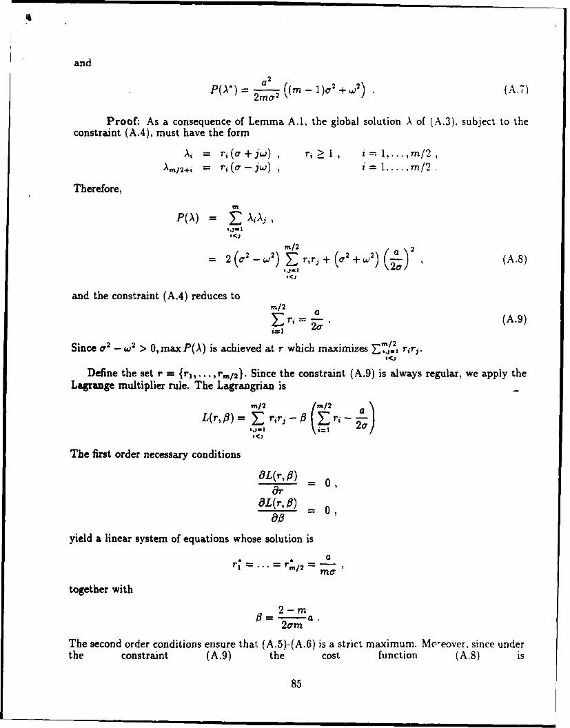
and

P(A-) = a ( ) ;2 (A\7)Q2m2

Proof: As a consequence of Lemma A.1, the global solution A of (A.3). subject to theconstraint (A.4), must have the form

Ai = ri((a+ jw) , ri1, i= 1,...,m/2,./2+i = ri(o -jw) , i = 1.. m/

Therefore,m

P(A) = AAj,,jm1 mo= 2 (2 W2)m/2 rr i ) 2( 8

2(oF,2 ,2(a8

and the constraint (A.4) reduces tom/2 a

Eri= (A.9)-- _ m/2

Since a2 W > 0, max P(A) is achieved at r which maximizes ,. r.

Define the set r = {rl,. ,r,/ 2 ). Since the constraint (A.9) is always regular, we apply theLagrange multiplier rule. The Lagrangrian is

m/2 m/2 a

L~~~r, ,, E irj- r

'<.2

The first order necessary conditions

aL(r,) 0ar

HL(r, )"-00

yield a linear system of equations whose solution is

ar , . . r ./2 = = - ,

together with

2-rm2am

The second order conditions ensure that (A.5)-(A.6) is a strict maximum. Me-eover, since underthe constraint (A.9) the cost function (A.8) is

85

II

quadratic, this maximum is the global maximum, and the proof is complete.Q.E.D.

Consider the optimization problem : For M even, and a.2 - 2 < 0, find a self conjugate setof eigenvalues A = {AE,...,AIE D(a. ..) such that

m

P(A) = Z i •,,, (A.10)6<J

is maximized subject toin

i=1

Ly emma A.3: The global solution AO = {AI,...,A,} of problem (A.10), (A.11) is givenby

*= (a + jw) , 1,...,m/2, (A.12)A =/2+i r*(a.-jw), :=1,...,m/2, (A.13)

where

2 =F (-m-1) and r =1, i = 2,..., m/2. (A.14)

In addition,

P(A) (2 02) (2 C2)( (A. 15)

Proof: As a consequence of Lemma A.1, the global solution A of (A.10), subject to theconstraint (A.11), must have the form

Ai = ri(a+ jw) , ri _ 1m , iAm/2+i = ri (a - jw) , im= ,...,rn2.

2 _ 2 .fn/2

Since a2 _ 2 < 0, and from (A.8), max P(A) is achieved at r which minimizes '.,.- rir,. Hence,

we need to determine the set r = {r,... r,/2} which minimizes

"'i/2P(r) = ri I$<J

subject to the constraints

ri _ 1, i=1,...,m/2, (A.16)m/2 rn

ri= •>_-. (A.17)

Since the constraints (A.16), (A.17) are regular, we apply the Karush-Kuhn-Tucker rule. The

Lagrangian is

Vn2 m/2 (M/2 aL(r,yf)- x r~r, - "/'(ri- 1)-/ r

=o 81 6k -5<)

86

where the non-negative Lagrange multiplier p-- [PI"" U,,/2] satisfies pi(ri - 1) = 0. for alli = 1,..., m/2. The first order necessary conditions yield a linear system of equations whosesolution generates a set of candidate extremal points given by

-l - k--- kri "-i 0• z"A(r

a= _ k'1, ikA(r), (A.1S)2r, = 1 , /•L=, zE A(r) ,

2a M-k2

where A(r) = {r : r = 1} is the set of active constraints and k < m denotes the number of activeconstraints. It can be shown that

(J..LM)2P(k)- P(k- 1)= 2a 2 < 02(m - k)(M + I - k)

Hence, among the candidate extremal points given by (A.18), the solution k = m/2 - 1 yieldsthe global minimum

a m

r = i = 2,.1..,m/2 ,

together with

17---1 ,2

=0,2 2 a i=2,...,m/2.

The results (A.12)-(A.15) then follow immediately. Q.E.D.

Consider the optimization problem: For m even, and a 2 - w2 > 0, find a set of self conjugateeigenvalues A = {Al,... ,A,.} E D(a,w) such that

'I'

P(A) = ] A•,A,, (A.19)ijeO

is maximized subject to

Ao = ro , ro> 1 (A.20)

= a. (A.21)iftiO

Lemma A.4: The global solution A* = {A*,...,A} of problem (A.19)-(A.21) is givenby

a - r0oaA: = (a +jw M 1, ... , m/2 ,mo"(~j)

.X•/÷, - a - roa (ar Mj ),i= 1..r/87o'

87

and

P(A') = ToO(a - roo) + ( a- roM)2 ( 1)02+W2)

Proof: From (A.20), the expression (A.19) can be expressed as:in

P(A) = E AA,6.)WO

= roa(a - rou) + ,AA. (A.22)msuI!,<J

Also the constraints (A.20) and (A.21) are equivalent to the following singleconstraint:

S, = a - roa. (A.23)

Since the first term in the right hand side of (A.22) is constant, the solution of the optimizationproblem (A.22), (A.23) is obtained from Lemma A.2. Q.E.D.

Consider the optimization problem : For m even, and a2 W w2 < 0, find a set of self conjugateeigenvalues A = {A,,. . . , A,,} E D(o,w) such that

YR

P(A) = E AAj, (A.24)s~jO

is maximized subject to

Ao = roa , roŽ1, (A.25)

Ai = a. (A.26)i=O

Lemma A.5: The global solution A* {A;,..., AI} is given by

A! = r,(o+jw), i=l...,m/2, (A.27)Aý/2+i = r'!(o- jw), i=1,...,m2, (A.28)

wherer• = 27r0 ( - 1) and r- 1, i = 2,..., m/2. (A.29)

In addition,

P(A') = ro°(a - rToo) + ( -2 or)(m-2) (m 2 - a -roor)

+ (W 2 + O2) (a )2 (A30)

Proof: The results (A.27)-(A.30) follow immediately from (A.22), (A.23), and LemmaA.3. Q.E.D.

88

APPENDIX A2: DERIVATION OF AVERAGED EQUATIONS FORHELICOPTER WITH VHHC

A2.1 AVERAGED EQUATIONS FOR HELICOPTER IN HC-.ERLet x, = ,= 0,X3 = i,X 4 = 0. Equations (4.21) and (4.22) are equivalent to

1, 0 r0 0

000 0

i3 0 0 M -+Vf n =ý2rot10

1 U (m 1 4m 2 -- I Sin+ *3) m 2 1~l]( ~m 2 -w•m3I12 Igt *)

i0 01 a X30X4

X -, 2 14 LC011 2 - kx,+.0s.nw- 3 + .sin,,w.).,- (')

-M2,,minX2 + OsinNwt - ,,M .,,-, +OURS, -- 7-.-.,)'" i)

X, X.) +. , 2X? X) .

The generating equation f20J for this case is

0 ]a sin

(-I +mj-m2•sn 2 z2)L -0 sin X. sin

d-r I(M 1+1112-?u2.1Y12Z2)

where r = i/c.We obtain the general solution of the above equation in the fast time r as

I =- Cl

2:2 = C2

-C( Cos 7

X3 = 2 + C3,m, + m 2 - m 2 sin C2

asin z2 COS T2:4 *'2 .r C

mI + M 2 - m 2 sin2 C2

where c,,i = 1,... ,4, are constants.Conser -ntly, the substitution for this case is

2:1 ZiI 2:2 Z2X2 Z2' + z h(r, z) ,

X3 MI +m.2-m min; ZZX4 j(,nj +M2 M i'm &m 2) "+r Z4

and the equation in Bogoliubov's standard form can be written as [20]:

-- = XdU,h(",z))

0 0 00 1 0 0

-2.is n s• n a aco o s i co 1 0 x

-2omrn2 sin 1 +rn2-mtun ÷-)

89

10 0 0

0 1 0 0

0 0 i *m 2 -ns2 X

0 Visans2

+M2 -ml M )

C(ml+m 2 --m3 &and '2) lfJta(ist .+1112 -1992 it 2)

-acetos + Z3SIn +m 2 -- M' Si3g '2

a s o n % C e 5 V + Z 4A1 nui+m2 Vm, sin) 52 )ka

[ (cfins ) coo ' + 24

-- 7219 gin 22+ 0 sin Nw --i(tr • mi:l::'n;'n'ni2 i ) + )J)

Therefore, applying the averaging principle , we obtain equations (4.23) and (4.24) where

Ti-= zand 72 = .

A2.2 AVERAGED EQUATIONS FOR HELICOPTER IN FORWARD FLIGHT

Let X2 = , X2 = X3 0, X4 = , s= , Z 6 = . Equations (4.4)-(4.6) are equivalent to:

1 0 0 0 0 0-zl0 1 0 0 0 0

-i2 0 0 1 0 0 0*3• " 0 0 O m .m- -mV cs t *l z e X

.i5 0 0 0 m i SCO• 1!m-m**•#

LzJ L +

-M2tZ+ COSZ3 - kzX1 + aO COGoin Wt- C -4-g in X(In2Anz- + 0iin N, gt -W9 ,

000

alpas (ms +m,-m, co*t .)m m,+m=, €. , a -c ,a .,,sim sinKPoll SR+U-) 01)

sin81cAoomemLE)-% in(is

The generating equation for this case is:

. 0

a 1`m `M2 -m cm 2 Xza) COS 06YII2 Gin X3 CM X3Si A iDS((ml +m2-m2.n2 mu+m) in n

X3- sin )s+m Sin+ X3 coO V3 coO , sin r11M1(?l+I'2).

dr •c M -1 sinr

where r = t/c.The general solution of the above equation is:

i - C1

X2 =C2

Z3 = C3

90

((MI + m 2 - M 2 COs: C3) cOsIP + M 2 sin c 3 cos c 3 sin 'j COST + C4=4 -aM,(m + M2)

Xs = -Ck (M((i +m 2 - m 2 sin c3) sinp +m 2 sin c3 cOs C3 cOS( + ) rs + cs.

mI(rn1 + Mn2 )(sin c3 cos COS C3 sincos r s/Iz•= ,) •cost + C6

where c•,i -= 1,... ,6, are constants.The resulting substitution is

X23 Z2

X3 Z3

- (fMl+M2-m2COS Z3)€co#+m2sinx3 coox3 sines COS" + Z4

X51 ( (ml +m2-m2 sin2 z3) sin IA.,2Sin Z, cOs 2SPCS c +sa(IrnZSCOSA+C Sm-) CMS +-O2X6 j sin z3 coos+cos z3sin A) COS '- +Z's

and the equation in Bogoliubov's standard form is [20]

1 0 0 0 0 00 1 0 0 0 000 1 0 0 0

- - i0 2x c #&-coo2az 3i 10i0 Xam 9 0 0 am2 , L CO 0 1 0 j "

0 0 o (Ai sl 2m SinJ-€s coo COS W•) coo r 0 1 0

100 0&OST 0 0 1

0 0 0 0 00 1 0 0 0 00 0 1 0 0 0

0wn 0W~.C* 0acal m Wa. +M% CO% aC4143 as" m Sin* Z"l(! 1 ,, 911) s a(ms•.ln Z)1

0 (1(-3m+ma2) ~ =8_ 7 ex

0 0 0 f'csa•÷ -- % sin 3 Bit -COOshMCs061m +1(-+)3 + )2. + )n) mn

( (+mI M- --in 2 cs 2 23)1cos p +Pm2 sins% cos Ba sm inp + COST

-Z -,m,(m 1,+ in) < o.+,

((n (m + m2 -M2sin 3) sin p+ msin2 •,s &a coos ! coo r COST

=-- -ro(m 1 + m 2) & €" -ks

Upnaplin h a ing psin c23 + ,ip, Nwe - n (in ) co n s (4.31) where - =and

where

tI Z4 rQM + M2 M2 COS cos 3) COS P + M2 sin Z3 COS Z3 sin u)a cos rMI(MI + M2)

t2 Z5 ((MIl + M2s -M2 sin 2 Z3) sin p + M2 sin z3 COS Z3 cos p)a• cos Tts = zs -MIlrn + M2)

Upon applying the averaging principle, we ,'%tain equations (4.31) where Tj -z v, and

91

Documents

DTIC · AcI-lo C oTA ... pitch angle control to ensure the desired altitude of the hovercraft and the high frequency rotor ... average zero scalar function,