Abstract

Random angle generation: modeling diffuse light reflection in planetary rings

by

Demitri A. Morgan

This work addresses the topic of generating random angles describing the scattered directions of

simulated photon packets within Monte Carlo ray-tracing simulations of planetary rings, such as that

of Salo and Karjalainen (2003), using an arbitrary reflectance law as the probability distribution and

not merely one describing a Lambert surface. Also, a computational method which accomplishes this

task, written in the Interactive Data LanguageTM , is developed and tested, using as the reflectance

law an experimental approximation (proposed by Cuzzi, 2008) to those derived in Hapke (1993)

describing photometric properties of surfaces having “large-scale roughness”. The method generates

the random angles with an implementation of the rejection sampling algorithm and uses polynomial

approximations of the reflectance law as comparison and squeeze functions, in addition to running

performance tests and a searching for approximations that yield higher performance.

Contents

1 Introduction 4

2 Geometric description of the problem 4

2.1 Notation and terminology . . . . . . . . . . . . . . . . . . . . . . . . . . . . . . . . . . . . . . 5

2.2 Coordinate basis . . . . . . . . . . . . . . . . . . . . . . . . . . . . . . . . . . . . . . . . . . . 6

2.3 The phase angle and luminance coordinates . . . . . . . . . . . . . . . . . . . . . . . . . . . . 8

2.3.1 Definitions . . . . . . . . . . . . . . . . . . . . . . . . . . . . . . . . . . . . . . . . . . 8

2.3.2 Transforming to phase angle and luminance coordinates . . . . . . . . . . . . . . . . . 9

2.3.3 Orientation . . . . . . . . . . . . . . . . . . . . . . . . . . . . . . . . . . . . . . . . . . 10

2.4 The sample space . . . . . . . . . . . . . . . . . . . . . . . . . . . . . . . . . . . . . . . . . . . 13

3 General description of the developed method 15

3.1 Rejection sampling . . . . . . . . . . . . . . . . . . . . . . . . . . . . . . . . . . . . . . . . . . 15

3.2 Modeling P ′ . . . . . . . . . . . . . . . . . . . . . . . . . . . . . . . . . . . . . . . . . . . . . . 16

3.3 Polynomial plane-sweep for bivariate trial point generation . . . . . . . . . . . . . . . . . . . 18

3.4 Performance testing . . . . . . . . . . . . . . . . . . . . . . . . . . . . . . . . . . . . . . . . . 19

4 Development and testing of a prototype angle generator 21

4.1 Input . . . . . . . . . . . . . . . . . . . . . . . . . . . . . . . . . . . . . . . . . . . . . . . . . . 21

4.2 Output testing and performance results . . . . . . . . . . . . . . . . . . . . . . . . . . . . . . 23

5 Conclusions 24

References 26

A Additional Figures and Tables 27

B Numerical techniques 29

B.1 Partial derivatives . . . . . . . . . . . . . . . . . . . . . . . . . . . . . . . . . . . . . . . . . . 29

B.2 Multi-dimensional Taylor expansions . . . . . . . . . . . . . . . . . . . . . . . . . . . . . . . . 30

B.2.1 Binomial expansion . . . . . . . . . . . . . . . . . . . . . . . . . . . . . . . . . . . . . 32

B.2.2 Multiplicity of Taylor series terms with a given set of powers . . . . . . . . . . . . . . 32

B.2.3 Constructing the sum . . . . . . . . . . . . . . . . . . . . . . . . . . . . . . . . . . . . 33

B.2.4 Implementation . . . . . . . . . . . . . . . . . . . . . . . . . . . . . . . . . . . . . . . . 34

B.3 Bivariate nonuniform sampling with a polynomial comparison function . . . . . . . . . . . . . 34

1

B.3.1 Generating ψ with the marginal distribution . . . . . . . . . . . . . . . . . . . . . . . 35

B.3.2 Generating µ with the conditional distribution . . . . . . . . . . . . . . . . . . . . . . 36

C Source Code 38

C.1 Functions . . . . . . . . . . . . . . . . . . . . . . . . . . . . . . . . . . . . . . . . . . . . . . . 38

C.1.1 Evaluation and re-expression . . . . . . . . . . . . . . . . . . . . . . . . . . . . . . . . 38

C.1.2 Setup and approximation . . . . . . . . . . . . . . . . . . . . . . . . . . . . . . . . . . 42

C.1.3 Trial point generation and rejection sampling . . . . . . . . . . . . . . . . . . . . . . . 44

C.1.4 Solving the quartic, cubic and quadratic equations . . . . . . . . . . . . . . . . . . . . 47

C.2 The SETUP procedure: . . . . . . . . . . . . . . . . . . . . . . . . . . . . . . . . . . . . . . . 49

C.3 The SEARCHSETUP procedure: re-implementation of SETUP . . . . . . . . . . . . . . . . . 53

C.4 Saving unformatted text data to files for plotting . . . . . . . . . . . . . . . . . . . . . . . . . 56

2

List of Figures

2.1 Figural description of a scattering event. . . . . . . . . . . . . . . . . . . . . . . . . . . . . . . 5

2.2 Inadequacy of phase angle and emitted angle to describe emitted ray direction . . . . . . . . 6

2.3 Figural display of luminance coordinates . . . . . . . . . . . . . . . . . . . . . . . . . . . . . . 8

2.4 Alternate orientations and corresponding luminance coordinates . . . . . . . . . . . . . . . . . 10

2.5 Incidence of a photon packet on a ring particle, assumed spherical. . . . . . . . . . . . . . . . 13

3.1 Rejection sampling (univariate example) . . . . . . . . . . . . . . . . . . . . . . . . . . . . . . 16

4.1 Affect of steepness and Minnaert parameters on the reflection law . . . . . . . . . . . . . . . . 22

4.2 Density plots of program output for A = 1, ν = 2 and i = π4 . . . . . . . . . . . . . . . . . . . 24

4.3 Performance at the optimal approximation starting point . . . . . . . . . . . . . . . . . . . . 25

A.1 Second, third, and fourth most efficient approximation starting points. . . . . . . . . . . . . . 27

3

1 Introduction

In early photometric modeling of planetary rings, the rings have been treated as semi-infinite, homogeneous

multilayers of particles, with each ring particle having a radius much less than the average distance to its

nearest neighbor (negligible or zero volume filling factor). The more recent work of Salo and Karjalainen

(2003) has taken the approach of removing the assumption of zero volume filling factor and using direct and

indirect ray tracing Monte Carlo method to model the scattering properties of the rings. The method treated

a region within a ringlet as a rectangular volume having horizontally periodic boundaries and spherical ring

particles much larger than the wavelength of visible light. By introducing simulated quanta of light (“rays”)

into the region which scatter into random directions at every intersection with the surface of a particle, and

recording the direction and “weight”1 of the escaping rays, the method simulates the directional distribution

of radiation reflected by Saturn’s rings. At each scattering, the random direction that a ray reflects into

is distributed according to Lambert’s reflectance law, which is uniform with respect to the azimuthal angle

(denoted φ in Salo and Karjalainen (2003) and ψ in Hapke (1993)) and utilizes the mathematical simplicity

of this model in the process of randomly generating the direction of the reflected ray. This work will address

the use of arbitrary reflectance laws in order to generalize the concept of photometric modeling by a Monte

Carlo ray tracing method.

2 Geometric description of the problem

The following conditions were imposed in the Monte Carlo method of Salo and Karjalainen (2003) and will

serve as the context of this work: denoting the local surface normal, incident ray vector and emitted ray

vector as n, e0 and e, respectively,

• Each ring particle is taken to have a regular and opaque surface; every time a ray intersects the surface

of an object, the scattered photon packet must not emerge from the inward side of the local tangent

plane, which can be likened to “below the local horizon” of the object. Formally, e0 ·n < 0 and e ·n > 0;

• The random direction that a simulated photon packet scatters into has a probability distribution that

is proportional to the reflection law.

• Ring particles in a simulated ringlet are similar in their composition, so that the reflection law and

surface albedo may be assumed to apply universally throughout the region.1To lessen the intensity of multiply scattered radiation, each simulated photon packet has an initial “weight” that is reduced

at each scattering.

4

• Surfaces of the ring particles do not contain any large-scale anisotropy, i.e. grain. Formally, for any

three angles π − i, e and g (see Section 2.1) that the three vectors n, e0 and e make with each other,

the reflection law function evaluated at them must be equal to the reflection law function evaluated at

the three angles π− i′, e′ and g′ that three other vectors F (n), F (e0), and F (e) make with each other

if i′ = i, e′ = e and g′ = g (F is in this case any orientation-preserving isometry of <3).

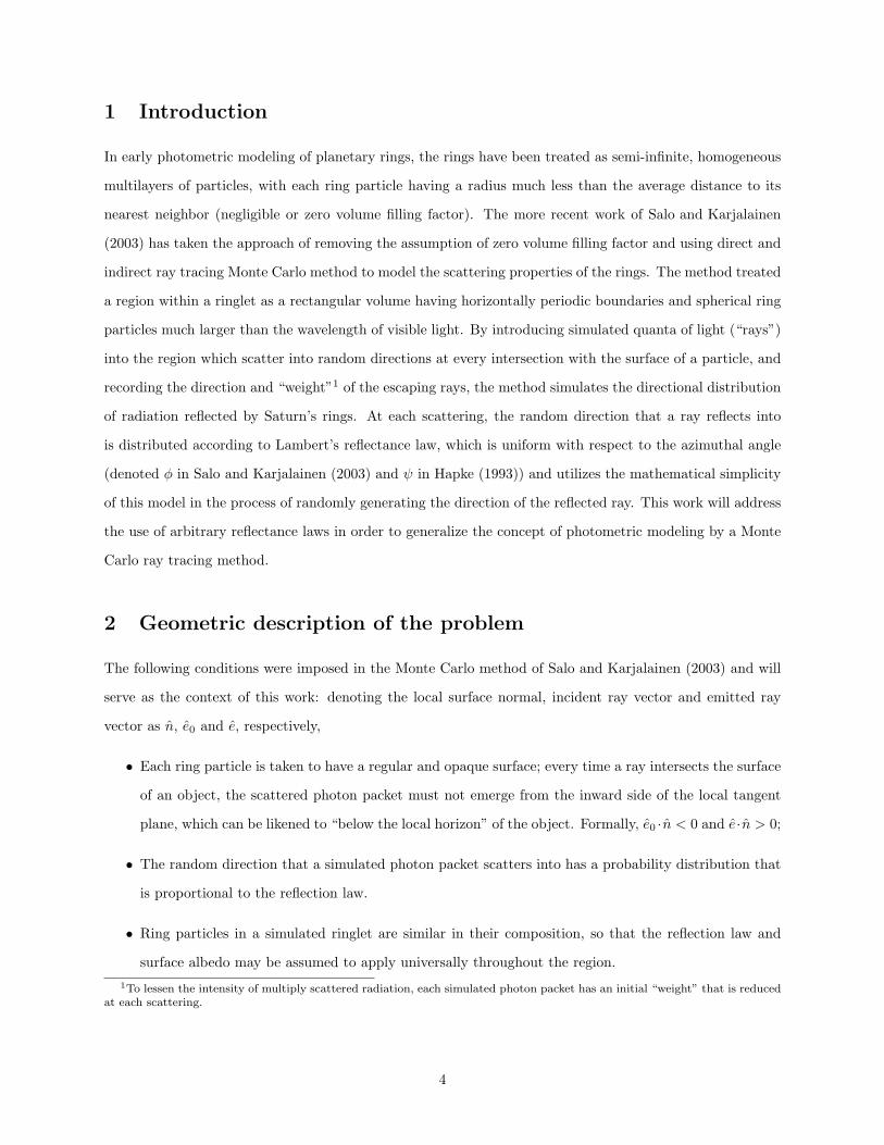
2.1 Notation and terminology

At each interaction of a simulated photon packet (“ray”) with the surface of a simulated ring particle,

referred to as an instance of reflection or a scattering event, the incident ray initially travels in the direction

e0 before the intersection. The vector pointing in the direction that the ray came from (denoted i ≡ −e0)makes an angle i with respect to the surface’s local normal vector, denoted n. After computing the value

of the parameter cos i (denoted µ0), which is the dot product i · n, the Monte Carlo method then passes

this value to the procedure that randomly generates the vector of the scattered ray’s direction, denoted e.

This vector is described by the two returned values, cos e (denoted µ) and ψ through an orthonormal basis

(Section 2.2), and these values are constrained to the intervals [0, 1] and [0, 2π] respectively; e is the angle

between e and n, so e, like i, must always lie within the interval [0, π2 ] as a direct result of the assumption

that the ring particles are opaque. The variable ψ is the angle between the projections of i and e to the local

tangent plane, as shown in Fig. 2.1. The sub-routine (a.k.a. the method) for generating random values of

Figure 2.1: Figural description of a scattering event. Here, the vector i is shown in place of e0.

µ and ψ will require a reflectance function, denoted P , to be assigned to it for use as the main reflectance

law. The method will assume that P only takes as its arguments angles that describe the directions of the

incident and emitted ray, which may include i, e, the angle between i and e (the phase angle, denoted g), or

5

the luminance coordinates L and Λ (see Fig. 2.3). In this project, the angles i, e and ψ will be used; they are

not dependent on one another and are well-defined for all orientations of n, i, e. Methods for transforming

between the values of µ0, µ, ψ and values of g, L, Λ are discussed in Section 2.3, and the reason for sampling

µ instead of e is given in Section 2.4.

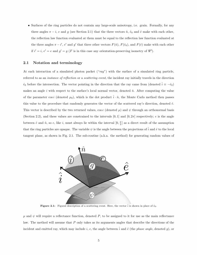
2.2 Coordinate basis

The task of generating random angles describing the scattered direction is made much simpler if the angles

are independent of one another, i.e. e and ψ as opposed to e and g (for example); in the latter case, not

only does the value of e affect the value of g and vice versa, but for any given i, e and g there are at least

two possible directions that these angles could describe, as shown by Fig. 2.2. Using cos e and ψ, not only

is it easier to fully express all directions, but the acceptable range of e can be directly imposed because

the sample space remains rectangular (having constant boundaries and linear independence between all

variables). While not all reflectance laws are explicit functions of i, e and ψ, methods for re-expressing such

functions in terms of i, e, ψ (see Section 2.3) may be used to accommodate them. Generating a random vector

Figure 2.2: For any given i, e, and g, there are at least two distinct possible e ∈ H that the three angles could correspondto, given n and i.

representing the scattered ray requires the construction of the vector using the values µ and ψ returned by

it and the components of the vectors e0 and n. This can be done by first constructing a local orthonormal

6

vector basis using i and n;

x′1 ≡ i− n cos isin i

(2.1a)

x′2 ≡ n× i

sin i(2.1b)

x′3 ≡ n (2.1c)

This basis can then be used to give an adequate description of vectors within the hemispherical set of

directions into which rays may reflect, denoted H. The emitted ray’s direction in the basis (x′1, x′2, x

′3) is

then:

e = (x′1 cosψ + x′2 sinψ) sin e+ x′3 cos e (2.2)

Or, using exclusively the returned values:

e = (x′1 cosψ + x′2 sinψ)√

1− µ2 + x′3µ

Using the expression of i and n in the coordinate basis of the simulation (x1, x2, x3) will then allow Definitions

2.1 and hence also the exit ray to be expressed in the same basis;

i = −e1x1 − e2x2 − e3x3 (ei denotes component i of e0)

n = = n1x1 + n2x2 + n3x3

∴ x′1 =1

sin i[(−e1 − n1 cos i) x1 + (−e2 − n2 cos i) x2 + (−e3 − n3 cos i) x3] ,

x′2 =1

sin i[(n3e2 − n2e3) x1 + (n1e3 − n3e1) x2 + (n2e1 − n1e2) x3]

x′3 = n1x1 + n2x2 + n3x3

Hence, the emitted ray expressed in the basis of the simulation is:

e =

(√1− µ2

sin i[(n3e2 − n2e3) sinψ − (e1 + n1 cos i) cosψ] + µn1

)x1

+

(√1− µ2

sin i[(n1e3 − n3e1) sinψ − (e2 + n2 cos i) cosψ] + µn2

)x2

+

(√1− µ2

sin i[(n2e1 − n1e2) sinψ − (e3 + n3 cos i) cosψ] + µn3

)x3

7

2.3 The phase angle and luminance coordinates

Some models of diffuse reflection, such as the brightness distribution of Akimov (1979), traditionally describe

reflectance on the surface of a spherical body and are functions of the luminance coordinates and/or the phase

angle. In order to have the option of using such functions as probability distributions, the phase angle and

luminance coordinates must be determined automatically given values of i, e, ψ, as described in Section 2.3.2,

so that the value of the reflectance function for any value of i, e, ψ (or µ0, µ, ψ) can be calculated. While it

may be possible to randomly generate the reflection solely in terms of these angles, it is far easier to use i, e

(or µ0, µ) and ψ to do so, as stated in Section 2.2, and hence doing so will not be addressed in this work.

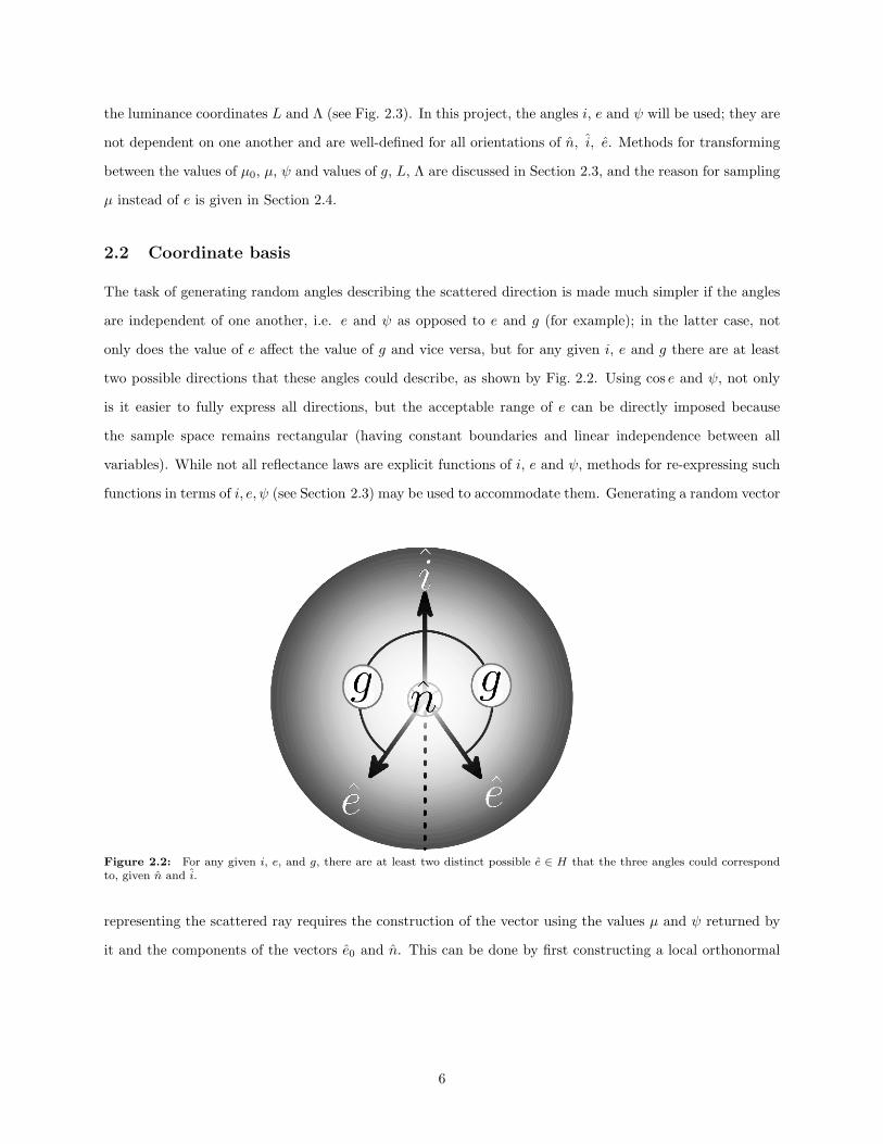
2.3.1 Definitions

Figure 2.3: (derived from Hapke, 1993, p.186) (L and Λ) with the angles i, e, ψ and g displayed in context. Light reflects offof a spherical body, and the luminance coordinates describe the position of the point of reflection on its surface (N) relative tothe plane spanned by i and e.

The phase angle, denoted g, and the luminance longitude and latitude, Λ and L (respectively) are as

shown in Fig. 2.3. The following formal definitions, based on similar definitions and notation from Hapke

(1993), will be used for these angles and the geometric elements on which their definitions are based:

• The photometric plane is the plane spanned by i and e whose intersection with the surface of the sphere

8

of solid angle is referred to as the luminance equator.

• The principal plane is the common plane that i, n, and e lie in if ψ = 0, 180◦, etc.

• The prime luminance meridian is the meridian in the direction of the observer (or, more generally, the

emitted ray), which runs through ^.

• The phase, either positive or negative, is determined by which side of the prime luminance meridian

the light source (À) is on, and the phase angle is the shortest angle from ^ to À along the luminance

equator.

• An angle along the luminance equator is negative if it runs clockwise (“West”), and positive if it runs

counterclockwise (“East”), where these directions are shown in the perspectives of Fig. 2.3 and Fig. 2.4.

• The luminance latitude (or photometric latitude), L, is the angle ∠NN ′ (the angle between the vector

n and its projection to the photometric plane).

• The luminance longitude (or photometric longitude), Λ, is the angle along the luminance equator

running from N ′ to the prime luminance meridian.

2.3.2 Transforming to phase angle and luminance coordinates

The phase angle and luminance coordinates are, as derived in Shkuratov et al. (2003) from Hapke (1993,

p.187),

g(i, e, ψ) = cos−1 (cosψ sin i sin e+ cos i cos e) (2.3a)

L(i, e, ψ) = cos−1

(√[sin (i+ e)]2 − (cosψ/2)2 sin 2e sin 2i

[sin (i+ e)]2 − (cosψ/2)2 sin 2e sin 2i+ (sin e)2(sin i)2(sinψ)2

)(2.3b)

Λ(i, e, ψ) = cos−1

(cos e

cosL(i, e, ψ)

)(2.3c)

Using these, the reflection law may be expressed entirely in terms of i, e and φ; if for example the func-

tion P it takes as its arguments g, L,Λ, it may be composed with these three functions as P (i, e, ψ) =

P [g(i, e, ψ), L(i, e, ψ),Λ(i, e, ψ)]. Although Equations 2.3b and 2.3c may suffice for most values of i, e, ψ,

they will result in indeterminate expressions for the anomalous cases ψ = 0 and i = e = 0. In order to

circumvent not-a-number errors, L can be assigned a value of 0 if ψ = 0 and/or i = e = 0; this is the result

of both the limiting case ψ → 0 and i = e→ 0. However, in spite of this safeguard, there is an inescapable

irregularity in L and Λ that results at zero phase angle regardless of how the luminance coordinates are set

up for this case. This is because when g = 0, the photometric plane is ill-defined; if two vectors are parallel,

9

then there is no unique plane that is parallel to both of them, and if g = 0 then e is parallel to i. More

specifically, the irregularity is that in the limiting case i = e 6= 0 and ψ → 0, L should equal i; the equality of

i and e results in a symmetry which causes the meridian running through N to be exactly halfway between

À and ^. This results in Λ = g/2 and, using the spherical law of cosines on 4ÀN ′N gives the expression

cos i = cosL cos g2 and thus L = cos−1(cos i/ cos g2 ). This translates to L = i for ψ → 0, and hence the value

of L (and by extension, Λ) in the limiting case g → 0 cannot be assigned a unique value. The consequence of

this is that a reflection law depending upon the luminance coordinates may possibly also be irregular around

zero phase angle.

2.3.3 Orientation

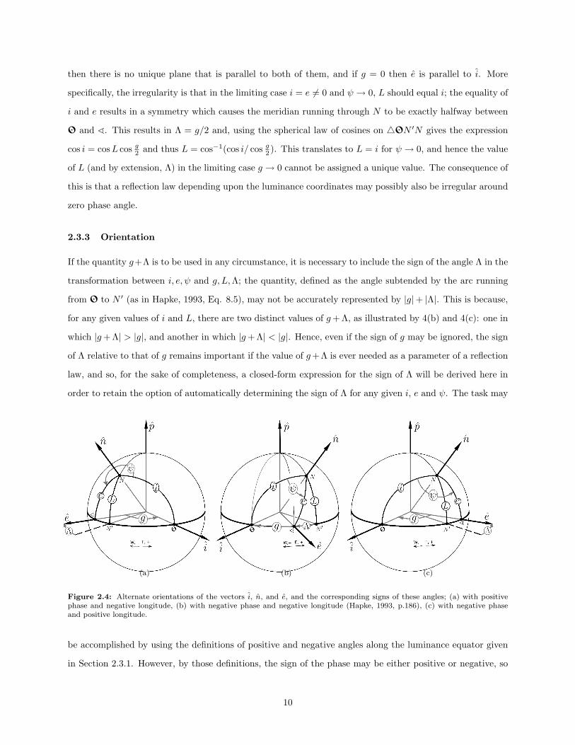
If the quantity g+Λ is to be used in any circumstance, it is necessary to include the sign of the angle Λ in the

transformation between i, e, ψ and g, L,Λ; the quantity, defined as the angle subtended by the arc running

from À to N ′ (as in Hapke, 1993, Eq. 8.5), may not be accurately represented by |g|+ |Λ|. This is because,

for any given values of i and L, there are two distinct values of g+ Λ, as illustrated by 4(b) and 4(c): one in

which |g+ Λ| > |g|, and another in which |g+ Λ| < |g|. Hence, even if the sign of g may be ignored, the sign

of Λ relative to that of g remains important if the value of g+Λ is ever needed as a parameter of a reflection

law, and so, for the sake of completeness, a closed-form expression for the sign of Λ will be derived here in

order to retain the option of automatically determining the sign of Λ for any given i, e and ψ. The task may

(a) (b) (c)

Figure 2.4: Alternate orientations of the vectors i, n, and e, and the corresponding signs of these angles; (a) with positivephase and negative longitude, (b) with negative phase and negative longitude (Hapke, 1993, p.186), (c) with negative phaseand positive longitude.

be accomplished by using the definitions of positive and negative angles along the luminance equator given

in Section 2.3.1. However, by those definitions, the sign of the phase may be either positive or negative, so

10

the sign of Λ relative to the phase is of greatest importance. To achieve this first requires determining East

and West along the luminance equator, and in this there is need for a third point of reference with which

to add perspective. This point must be N ; the vectors i and e do not adequately describe the orientation

of the photometric plane, but only the luminance axis (which runs perpendicular to it). The photometric

plane’s positive normal, p, may then be defined as follows: let it be parallel (or anti-parallel) to e × i, and

let it be such that p · n > 0, or in other terms, let N always be “North” of the luminance equator, and the

quantity L always positive. With these assumptions in place, the positive normal p (the “North luminance

pole”) can be explicitly written as follows:

p = sign[n ·

(e× i

)] e× i

|sin g| (2.4)

To first obtain the sign of g, one can begin by considering how ^ being East of À will result in the vector

e× i pointing “North”, and how the opposite arrangement will result in it pointing “South”. It then becomes

clear that the sign of sin g (and hence also the sign of g)2 is related to the orientation of the three vectors i,

e and n as follows:

sign[sin g] = sign[p ·

(e× i

)](2.5)

Then, using Equation 2.2 and Equation 2.4 along with definitions 2.1, this value can be examined and

simplified by expressing each part of it in terms of i and n; first, the quantity n ·(e× i

)can be reduced to

an expression containing familiar angles;

n ·(e× i

)= n ·

[(x1 × i cosψ + x2 × i sinψ

)sin e+ x3 × i cos e

]

= n ·

−n× i

sin icosψ +

(n× i

)× i

sin isinψ

sin e+

(n× i

)cos e

= n ·[(n× i

)× i

] sinψ sin esin i

= n ·(i cos i− n

) sinψ sin esin i

= − sin i sin e sinψ

Since i and e are positive, this implies

sign[n ·

(e× i

)]= sign(− sinψ)

2The constraint 0 ≤ |g| ≤ π directly follows from the assumption that neither i nor e can be greater than π2; g cannot be

greater than i+ e. This implies that the sign of sin g is the same as the sign of g.

11

Using this result, Equation 2.5 then reduces to:

sign(g) = sign(− sinψ) (2.6)

Next, to obtain the sign of Λ, one can similarly begin by considering the conditions under which it will be

positive and negative, and assigning to Λ the sign of the dot product between p and some vector characteristic

of it. The vector in question is n × e; by inspection of Figures 2.4, this vector should point South of the

luminance equator whenever Λ is negative, and North of it whenever Λ is positive. Using this principle, the

sign of the longitude can be then be written explicitly:

sign(Λ) = sign (p · (n× e))

In this case, simplifying this expression will first require expressing e × i in terms of i and n, again using

Equation 2.1, 2.2, and 2.4, and then simplifying:

e× i =

[(− cos isin i

)n× i

]cosψ +

(n× i

)× i

sin i

sinψ

sin e+ n× i cos e

= (cos e− cosψ cot i sin e) n× i+ (− sinψ csc i sin e)n+ (sinψ cot i sin e) i

Next, performing the same for n× e:

n× e = sin e[cosψ cos i

sin in× i+

sinψsin i

n×(n× i

)]

= sin e[(cosψ cot i) n× i+ (sinψ cot i) n+ (− sinψ csc i) i

]

Finally, the dot product between them may be obtained by considering how i · n = cos i, and (n× i) ·(n× i) =

sin2 i, and how all other terms will be zero;

p · (n× e) =sign(− sinψ) sin e cos i

|sin g|

[cosψ (cos e− cosψ cos i sin e) +

(sinψsin i

)2

(cos e− 1)

]

Hence, eliminating a factor of sign(g) and all the factors of positive quantities from this expression gives the

sign of Λ relative to g:

sign(Λ) = sign

[cosψ (cos e− cosψ cos i sin e) +

(sinψsin i

)2

(cos e− 1)

](2.7)

12

2.4 The sample space

As in Salo and Karjalainen (2003), this project will adopt the convention that P is a conditional probability

distribution of the values of (µ0;µ, ψ) instead of the values of (i; e, ψ). This avoids the bias in probability

density caused by the transformation between points (en, ψn) in the domain D* ≡ [0, π2 ]× [0, 2π] and points

en in H. To illustrate this effect, consider how a uniform reflection law, being constant with respect to e and

ψ (P = 12π for example), should generate isotropically distributed ray vectors in H, each associated with e

and ψ through the parameterization given by Equation 2.2. Then, N points of (en, ψn) ∈ D* corresponding

to N uniform points en ∈ H will have a non-uniform density that is proportional to sin e. This is because

the (average) number of points contained within an area element de dψ ⊂ D* corresponding to points

contained in a surface element dA ⊂ H will be N2πdA sin e de dψ (where A ⊂ B denotes “A is a subset

of B”). Conversely, a uniform density of points in (e, ψ) will translate to a non-uniform density of points

on the hemisphere; points will be “compressed” at lower values of e due to the lesser range of positions

that variation of ψ can result in. This may be remedied by generating values of e with probability density

proportional to sin e, and if the transformation law of probabilities (Press et al., 2007, p.363) is used, the

resulting method is essentially identical to sampling a value of µ uniformly in the interval [0, 1] and then

treating e as cos−1 µ. Furthermore, a similar change of variables may be adopted for the incident angle i

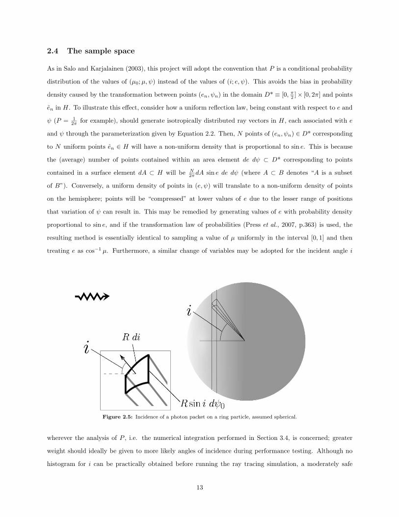
Figure 2.5: Incidence of a photon packet on a ring particle, assumed spherical.

wherever the analysis of P , i.e. the numerical integration performed in Section 3.4, is concerned; greater

weight should ideally be given to more likely angles of incidence during performance testing. Although no

histogram for i can be practically obtained before running the ray tracing simulation, a moderately safe

13

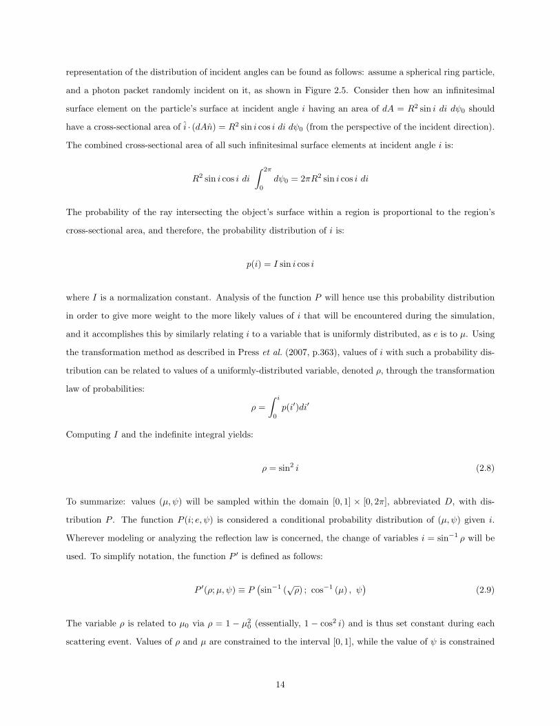
representation of the distribution of incident angles can be found as follows: assume a spherical ring particle,

and a photon packet randomly incident on it, as shown in Figure 2.5. Consider then how an infinitesimal

surface element on the particle’s surface at incident angle i having an area of dA = R2 sin i di dψ0 should

have a cross-sectional area of i · (dAn) = R2 sin i cos i di dψ0 (from the perspective of the incident direction).

The combined cross-sectional area of all such infinitesimal surface elements at incident angle i is:

R2 sin i cos i di∫ 2π

0

dψ0 = 2πR2 sin i cos i di

The probability of the ray intersecting the object’s surface within a region is proportional to the region’s

cross-sectional area, and therefore, the probability distribution of i is:

p(i) = I sin i cos i

where I is a normalization constant. Analysis of the function P will hence use this probability distribution

in order to give more weight to the more likely values of i that will be encountered during the simulation,

and it accomplishes this by similarly relating i to a variable that is uniformly distributed, as e is to µ. Using

the transformation method as described in Press et al. (2007, p.363), values of i with such a probability dis-

tribution can be related to values of a uniformly-distributed variable, denoted ρ, through the transformation

law of probabilities:

ρ =∫ i

0

p(i′)di′

Computing I and the indefinite integral yields:

ρ = sin2 i (2.8)

To summarize: values (µ, ψ) will be sampled within the domain [0, 1] × [0, 2π], abbreviated D, with dis-

tribution P . The function P (i; e, ψ) is considered a conditional probability distribution of (µ, ψ) given i.

Wherever modeling or analyzing the reflection law is concerned, the change of variables i = sin−1 ρ will be

used. To simplify notation, the function P ′ is defined as follows:

P ′(ρ;µ, ψ) ≡ P(sin−1 (

√ρ) ; cos−1 (µ) , ψ

)(2.9)

The variable ρ is related to µ0 via ρ = 1 − µ20 (essentially, 1 − cos2 i) and is thus set constant during each

scattering event. Values of ρ and µ are constrained to the interval [0, 1], while the value of ψ is constrained

14

to [0, 2π]. The domain [0, 1]× [0, 1]× [0, 2π] in which triplets (ρ, µ, ψ) exist is abbreviated D′.

3 General description of the developed method

The method, summarized in this section, takes the same essential form of a universal generator as described

in Horman et al. (2003); in order to generate random sample points according to an arbitrarily-chosen

distribution, it utilizes the rejection sampling algorithm, and automatically self-optimizes to the distribution

in use during an initial setup procedure which, although computationally expensive, only needs to be executed

once for each distinct P ′. The initial performance cost (a.k.a. the setup time) of doing so will be negligible if

the number of reflections in the ray-tracing simulation is considerably large; reducing the marginal execution

time (the time required to generate one random pair of µ, ψ) is more important than reducing the setup

time when the sampling algorithm will be used a large number of times (Horman et al., 2003, p.5).

3.1 Rejection sampling

The rejection sampling method will generate random pairs of (µ, ψ) with probability density P ′ by first

generating trial points of (µ, ψ) within the sample space (D) distributed according to a comparison function,

denoted fc (which must always be greater than or equal to P ′), and a third uniformly-distributed random

deviate (referred to here as the trial gauge, and denoted r) in the interval between zero and the value of fc.

However, triplets (µ, ψ, r) such that r does not have a value less than P ′ (as illustrated by the univariate

example depicted in Fig. 3.1) are rejected in favor of trying to generate a new trial point and trial gauge.

Points (µ, ψ, r) that are not rejected will in this way be distributed uniformly in the space contained beneath

the function P ′ (a subset of D ×<+), and the values of µ and ψ (their “shadows” in D) will be distributed

according to P ′ (Horman et al., 2003, p.17,18). The general structure of the rejection sampling algorithm

(using a “squeeze function”) is as follows:

1. Generate random values of µ and ψ using a polynomial comparison function or a constant, in either

case denoted fc.

2. Generate r uniformly in the interval [0, fc(ρ;µ, ψ)] (where ρ is a pre-determined value in each instance).

3. Evaluate the squeeze function (denoted fs). The squeeze function must always be less than the dis-

tribution P ′, and is meant to improve efficiency by being less expensive to execute than P ′ (see “The

Squeeze principle” in Horman et al., 2003, p.20).

4. If: r < fs(ρ;µ, ψ) close the loop and return the values of the trial point;

15

(a) (b)

Figure 3.1: (a) (Adapted from Landau and Paez, 2004, p. 108): Rejection sampling with a constant: generate a randomdeviate uniformly within the domain, and then another (the “trial gauge”) between zero and some value that is greater than thedistribution within the domain; reject if it is greater than the distribution evaluated at the first random value, accept otherwise;(b) (Adapted from Press et al., 2007, p. 366): Rejection sampling using a comparison function: generate a random deviatewithin the domain according to a comparison function, and then generate the trial gauge between zero and the value of thecomparison function evaluated at the trial point value, and perform a similar test as with the constant.

Else if: r < P ′(ρ;µ, ψ) close the loop and return the values of the trial point;

Else Start over at step 1.

3.2 Modeling P ′

The purpose of the comparison function is to reduce the volume containing points that must be rejected.

This yields a gain in performance (Horman et al., 2003, p.22) depending on how much volume is eliminated

by the function and how costly it is to perform trial point generation with it. To create comparison and

squeeze functions to loosely mimic the shape of P ′, the method uses Taylor series expansions, and the

means of performing this is described in greater detail in Appendix B.2. Although the method can in

theory be generalized to arbitrary order, the approximations will be limited in this project to 3rd order due

to the limitations of achieving higher-order numerical derivatives with sufficient accuracy. The orders of

approximation will be denoted mc for the comparison and ms for the squeeze function.

While the Taylor series may in some cases provide a moderately reliable polynomial approximation to

the distribution P ′, there is never any guarantee that it will always remain greater than (or, for the squeeze

function, less than) the distribution function P ′. Securing this is essential to having functions fc and fs that

work properly; as stated in Section 3.1, the comparison function must always be greater than P ′, and the

squeeze function must always be less than P ′. To correct for the imperfections of Taylor approximations,

the initialization process will run a “safety” test/adjustment on each of the polynomials. This procedure

works as follows (with p denoting a generic power series approximation):

Before testing: Define three new objects:

16

• A function (denoted d) that computes p(ρ;µ, ψ)− P ′(ρ;µ, ψ)

• A function (denoted −d) that computes P ′(ρ;µ, ψ)− p(ρ;µ, ψ)

• A 19-component vector of double-precision numbers (denoted ∆c here)

• Another 19-component vector of doubles, ∆s

Main testing procedure: For each order m, from 2 to 20, perform the following tasks:

1. Use the IDL function AMOEBA to compute the minimum of d within D′, and store the returned

value in ∆c[m− 2];

2. Again use AMOEBA to compute the minimum of −d within D′, and store the returned value in

∆s[m− 2];

Result: The array ∆[l,m− 2] corresponds to corrections that must be subtracted from the 0th-order power

series term of each mth order Taylor approximation, for m from 2 to 20, so that that the comparison

functions are always greater than, and the squeeze functions always less than, the function P ′ within

the domain D′.

In light of this method for making the polynomial approximations safe for use as comparison/squeeze func-

tions, an important consideration in assessing the efficacy of using polynomials (especially Taylor series

approximations) is how big of an adjustment must be made, because a larger adjustment will adversely af-

fect the performance of the trial point generator; the direct consequence is that a larger volume of points will

have to be rejected. As mentioned in Section 2.3.2, irregularities may exist in the distribution around i = e

and ψ = 0 (zero phase angle), and while this is to be expected (because of the spike in luminosity caused by

the opposition effect; see Hapke (1993, pp.216-235)) it will have the possible consequence of making the ran-

dom number generation process inefficient and problematic because of the difficulty of creating polynomials

modeled after the shape of the reflection law. A sharper opposition spike thus may translate to the rejection

of a high if not higher volume of trial points than would result from using a constant/uniform comparison

function, especially if the necessary adjustments are large. Although multivariate transformed density re-

jection, as described in Horman et al. (2003), may possibly be able to avoid this problem by constructing a

polytope-shaped comparison function out of hyperplanes tangent to the convex density-transformed distri-

bution, the implementation of that method is not covered in this project. Instead, given that it is possible to

test whether using a polynomial is more or less efficient than using a constant (by the method described in

Section 3.4), the chosen approach to random deviate generation is to test whether or not a simple polynomial

comparison function can offer a better performance, and to use one if it does.

17

3.3 Polynomial plane-sweep for bivariate trial point generation

Trial point generation is in essence the sampling of points uniformly within a region that has one dimension

more than the number of variables being generated by the rejection process, as depicted in Fig. 3.1. In

this project, the chosen method for accomplishing this will employ the same principle as the sweep-plane

technique discussed in Horman et al. (2003), but this principle will be used on the volume contained be-

neath a polynomial comparison function instead of a polytope. By generating the first of the two random

variables according to the marginal distribution3, the second variable can then be generated according to

the conditional distribution that results from fixing the value of the already-generated first variable and the

predetermined value, ρ. During each step of this process, the method will utilize the transformation law of

probabilities (Press et al., 2007, p.363), and this requires the cumulative distribution, which is the indefinite

integral of a distribution, to be determined from the marginal/conditional distributions of µ and ψ. For the

first variable, ψ, the transformation law reads:

∫ 1

0

∫ ψ

0

fc(ρ;µ, ψ′) dψ′ dµ = R[0, 1] ·∫ 1

0

∫ 2π

0

fc(ρ;µ, ψ) dψ dµ (3.1)

This can be interpreted as sweeping a plane through D in the direction of ψ until reaching an amount of

volume under fc that is uniformly distributed between zero and the total volume under fc in D (given a

value of ρ). After solving this equation for ψ, the problem of generating the next random variable, µ, reduces

to the univariate case of obtaining a random value by the transformation method, and is essentially the same

as depicted in Figure 1(b);

∫ µ

0

fc(ρ, ψ;µ′) dµ′ = R[0, 1] ·∫ 1

0

fc(ρ, ψ;µ) dµ (3.2)

Now, because the comparison function is a finite power series of ρ, µ and ψ, the indefinite integral of

such a function with respect to any of the three variables should also be a finite power series. Arranging

the polynomial coefficients by the order of the term they correspond to thus optimizes this process and

ensures that no redundant operations are performed (see Appendix B.2). Furthermore, in this project, no

approximations higher than order 3 are used, which allows the use of the analytical solutions to the quartic,

cubic and quadratic equations (as described in Abramowitz and Stegun, 1970, pp.17-18) to solve for values

of µ and ψ and thus generate them via the transformation method.3The marginal distribution is the result of integrating the comparison function over all possible values of the second variable

(Feller, 1970, p.67).

18

3.4 Performance testing

The setup procedure not only creates comparison functions, but also a test of performance for each order of

approximation. To demonstrate how it accomplishes this, consider first how the execution time of a process

is essentially the sum of the execution times of all sub-processes, and how if any process is repeated, its

contribution to the total execution time is expected to be the product of the time it takes to execute once

and the average number of times it must be executed. Next, it may be noted that the average total number

of trial points that will be needed is equal to twice the value of the rejection constant (Horman et al., 2003,

p.22), and in the case of this project, this value (denoted N) is equal to:

N = 2

∫D′ fcdV∫D′ P

′dV(3.3)

(in this case, dV = dρ dµ dψ). The test of efficiency will also require knowing how many times (on average)

that P ′ will have to be evaluated versus how many trial points total will be necessary, since the squeeze

function is expected to be less costly than P ′ to evaluate. Using the formula for this value from Horman et al.

(2003, p.22), it should be in this case:

NP ′ =

∫D′ fc dV − ∫

D′ fsdV∫D′ P

′dV=N

2−

∫D′ fsdV∫D′ P

′dV(3.4)

Using these numbers of repetitive executions, the average total amount of computational resources required to

find one point by rejection sampling can thus be determined by revisiting and examining the generic algorithm

for rejection sampling (in Section 3.1), and assigning to each operation an amount of time consumed in its

execution, denoted O(operation), and then multiplying by the average number of times that it will be

executed. One iteration of the algorithm requires:

• Generation of a trial point, with trial gauge: O(trial)

• An execution of the squeeze function: O(fs)

• Comparison of two double-precision numbers: O(test)

• (If the trial gauge was not less than the squeeze function):

– An execution of the distribution function: O(P ′)

– A comparison of two double-precision numbers: O(test)

19

Hence, the generation of one point using a polynomial, denoted as the operation poly, requires (on average):

O(poly) = N∗ [O(trial) +O(fs) +O(test)] +NP ′∗ [O(P ′) +O(test)] (3.5)

Then, using the definitions:

IP ′ ≡∫

D′P ′dV

Ic ≡∫

D′fc dV

Is ≡∫

D′fs dV

Also, with the abbreviated notation:

O(pre) ≡ O(trial) +O(fs) +O(test)

O(exe) ≡ O(P ′) +O(test)

Equation 3.5 can then be re-constructed for the performance test as follows:

O(poly) =Ic

2IP ′·O(pre) +

Ic − IsIP ′

·O(exe) (3.6)

If a constant is being used instead of the polynomial trial point generator, the quantity will be:

O(const) =πMax(P ′)

IP ′·O(pre) +

2πMax(P ′)− IsIP ′

·O(exe)

Thus, by performing the integral IP ′ and the integrals Ic and Is (for each mc and ms) using the IDL function

INT 3D, and then running the PROFILER procedure to determine O(pre) and O(exe), setup computes the

marginal execution time of the rejection sampling algorithm for each of the trial point generators available.

Furthermore, since the method of approximation used to generate comparison functions permits the use

of any arbitrary starting point within the domain D′, the overall initialization procedure can perform a

cursory search over D′ for a good approximation by picking several random points, performing the setup

and performance testing for each point, and then picking the best comparison function out of all those

available at the end of the search.

20

4 Development and testing of a prototype angle generator

Throughout the development process, various adjustments and accommodations were found necessary in

order to circumvent the various difficulties that were encountered:

A search over the sample space; given the arbitrary shape of the function and the limit of approxima-

tions to 3rd order, it was at a later time in this project deemed appropriate to make use of the flexibility

of the approximation method to search for better approximation starting points.

Adaptive precision and maximum iterations; For phase functions having a more pronounced opposi-

tion peak, the maximization routine AMOEBA often failed to converge to the desired precision due to

the irregular shape of the function. The step taken to circumvent this was to set the precision and

iterations to initial values, and then reduce the precision/increase the maximum number of iterations

until the function converged, and to afterwards make an additional safety correction to the maximum

by multiplying the result by (1 + precision), where precision is increased in each iteration but is not

allowed to exceed 10−1. The procedure then quits if amoeba still fails to converge.

Use of analytical solutions to polynomials; because of the restriction of the comparison functions to

3rd order and lower, the cumulative distributions were limited to 4th order and lower, which serendipi-

tously permitted use of the analytical solutions to the quartic and cubic equations. The benefit of using

them is in their efficiency and safety; the analytical solutions give a much more straightforward path

to computing the roots with very high precision in very few operations, as opposed to the polynomial

root-finding function FZ ROOTS. The latter function, which uses Laguerre’s method to determine the

roots, was an option explored in the earlier stages of development, but it was found to be unreliable

for use in automatic procedures called upon very frequently, since it would occasionally return null and

throw the error that it failed to converge to the desired precision.

Organized retention of all setup constants: the procedure stores all constants created by the setup at

each point within a structure declared within a common block shared between functions associated

with trial point generation, so that in any larger ray-tracing simulation, the optimal setup remains

available for use.

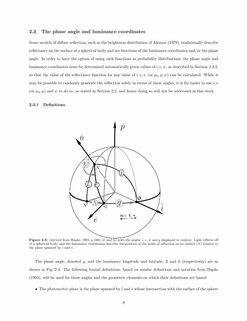
4.1 Input

The method described throughout section 3, which in this project has been implemented in IDL, used the

following function (J. Cuzzi, personal communication, 2008) as its probability distribution during all of the

21

-3 -2 -1 1 2 3Ψ

0.05

0.10

0.15

0.20

0.25

0.30

0.35

PH45°;45°,ΨL

(a) scale=0.8

0.5 1.0 1.5e

0.1

0.2

0.3

0.4

0.5

0.6

0.7

PH45°,e,0°L

(b) scale=0.8

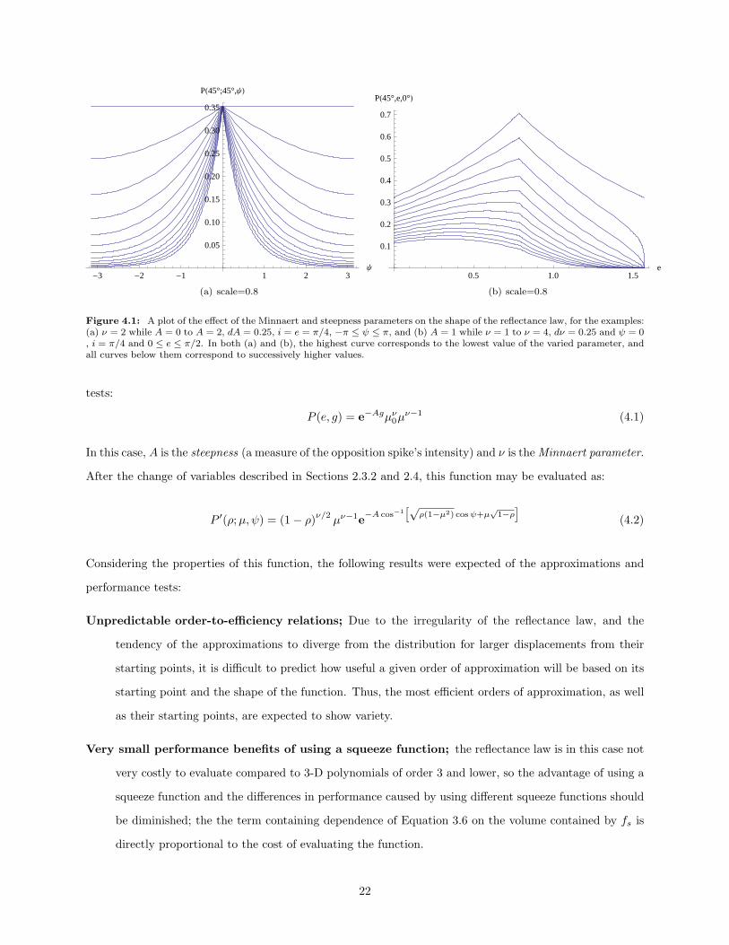
Figure 4.1: A plot of the effect of the Minnaert and steepness parameters on the shape of the reflectance law, for the examples:(a) ν = 2 while A = 0 to A = 2, dA = 0.25, i = e = π/4, −π ≤ ψ ≤ π, and (b) A = 1 while ν = 1 to ν = 4, dν = 0.25 and ψ = 0, i = π/4 and 0 ≤ e ≤ π/2. In both (a) and (b), the highest curve corresponds to the lowest value of the varied parameter, andall curves below them correspond to successively higher values.

tests:

P (e, g) = e−Agµν0µν−1 (4.1)

In this case, A is the steepness (a measure of the opposition spike’s intensity) and ν is the Minnaert parameter.

After the change of variables described in Sections 2.3.2 and 2.4, this function may be evaluated as:

P ′(ρ;µ, ψ) = (1− ρ)ν/2 µν−1e−A cos−1h√

ρ(1−µ2) cosψ+µ√

1−ρi

(4.2)

Considering the properties of this function, the following results were expected of the approximations and

performance tests:

Unpredictable order-to-efficiency relations; Due to the irregularity of the reflectance law, and the

tendency of the approximations to diverge from the distribution for larger displacements from their

starting points, it is difficult to predict how useful a given order of approximation will be based on its

starting point and the shape of the function. Thus, the most efficient orders of approximation, as well

as their starting points, are expected to show variety.

Very small performance benefits of using a squeeze function; the reflectance law is in this case not

very costly to evaluate compared to 3-D polynomials of order 3 and lower, so the advantage of using a

squeeze function and the differences in performance caused by using different squeeze functions should

be diminished; the the term containing dependence of Equation 3.6 on the volume contained by fs is

directly proportional to the cost of evaluating the function.

22

Slow apparent convergence to the true density; although points sampled using the resulting trial point

generator will be properly distributed according to the reflectance law, the density will appear to con-

verge to the true density rather slowly because a very small bin size will be needed to properly gauge

the density of points near points where there is a high amount of variation in the density, i.e. near

opposition.

The parameters A and ν were set to 1 and 2, respectively, for this test. As demonstrated in Fig. 4.1, these

two values should correspond to a slightly pronounced opposition peak, and greatly diminished intensities

at lower emitted angles, while lower values of the steepness and Minnaert parameter should result in the

reflection law having a less irregular shape. For that matter, it is reasonable to conclude that the performance

of the method for values of A less than the values at which the method is benchmarked should be greater;

as explained in Section 3.2, a more highly irregular distribution will require greater safety adjustments to be

made, resulting in lower performance. Setting A = 1 therefore provides a rough measure of the minimum

performance for all values of A lower than 1, although this choice has been made arbitrarily nevertheless.

4.2 Output testing and performance results

To ensure that the algorithm successfully generates random values with proper density, a cursory test of it was

performed by generating large quantities of random points for a given incident angle (π/4) and observing

the count of points in an array of bins, shown in Fig. 4.2. Furthermore, at the end of the SEARCHSETUP

procedure, which performed a survey of approximations taken at 20 uniformly-sampled points (“x0”) in the

domain D′, four sets of approximations were chosen for display purposes. While the performances of these

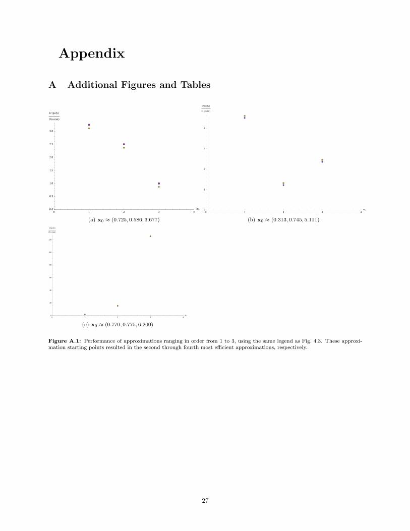
approximations, displayed in Fig. 4.3 and Fig. A.1, are not all very good, they each contain a best point, and

for each of the four sets of approximations chosen, the best approximations in the set correspond to one of the

four most efficient trial point generators in the survey. These results are directly in line with expectations;

the starting points that yielded the four most efficient trial point generators are not particularly close to

one another, and the best order of approximation differs for each point, along with relations between order

of approximation and performance that are also different for each point. The setup procedure succeeded in

finding a useful approximation; at the starting point (0.866, 0.412, 6.037), the approximation orders mc = 3

and ms = 2 resulted in the performance:

O(poly)O(const)

= 0.472707

This corresponds to a better trial point generator than a uniform one; the marginal execution time for this

polynomial comparison/squeeze function combination is less than half that of the former.

23

(a) 104 points (b) 2.5× 105 points

(c) 106 points (d) Equation 4.2

Figure 4.2: Program output as a density plot of points, using 50 bins in each dimension, with A = 1, ν = 2 and i = π4. To

display the opposition spike in the center of each plot, the bins were transposed in their values of the ψ coordinate using thebranch cut −π ≤ ψ ≤ π. Note the slow convergence to the function in Equation 4.2

5 Conclusions

It has been demonstrated that, for a reflection law with steepness less than or equal to unity, it is possible

to achieve better performance of the rejection sampling algorithm with polynomial approximations as com-

parison functions, even with a moderately unreliable method of approximating, than with using a uniform

comparison for generating trial points; using a moderately small survey of points, optimal comparison func-

tions can be found. Additional measures not covered in this work that could be taken to find even more

efficient comparison functions include searches around each of four optimal approximation points, or an en-

tirely different method of polynomial approximation that is more reliable than the Taylor expansion; insofar

as it is trivial to obtain analytical expressions for the cumulative and marginal distributions from a 3-variable

polynomial (per the method described in Section B.3), most of the the techniques used in this project may

24

æ

æ

æ

à

à

à

ì

ì

ì

0 1 2 3 4mc

1

2

3

4

5

6

O HpolyL

O HconstL

ì ms=3

à ms=2

æ ms=1

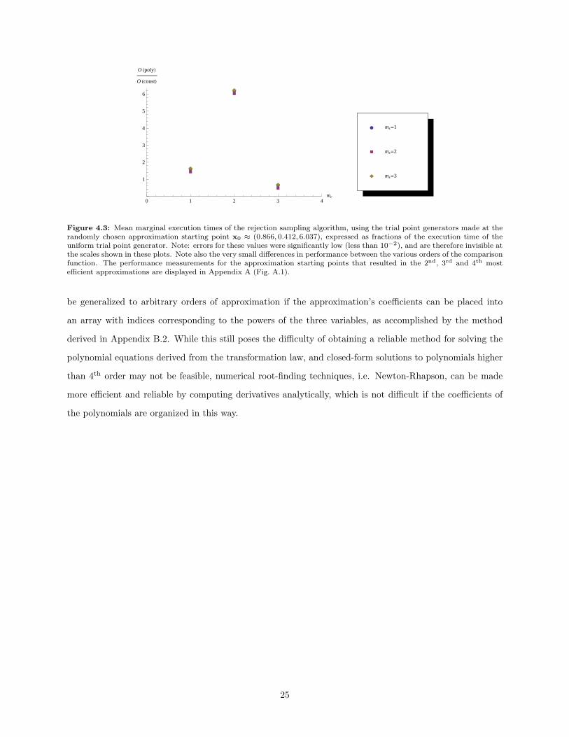
Figure 4.3: Mean marginal execution times of the rejection sampling algorithm, using the trial point generators made at therandomly chosen approximation starting point x0 ≈ (0.866, 0.412, 6.037), expressed as fractions of the execution time of theuniform trial point generator. Note: errors for these values were significantly low (less than 10−2), and are therefore invisible atthe scales shown in these plots. Note also the very small differences in performance between the various orders of the comparisonfunction. The performance measurements for the approximation starting points that resulted in the 2nd, 3rd and 4th mostefficient approximations are displayed in Appendix A (Fig. A.1).

be generalized to arbitrary orders of approximation if the approximation’s coefficients can be placed into

an array with indices corresponding to the powers of the three variables, as accomplished by the method

derived in Appendix B.2. While this still poses the difficulty of obtaining a reliable method for solving the

polynomial equations derived from the transformation law, and closed-form solutions to polynomials higher

than 4th order may not be feasible, numerical root-finding techniques, i.e. Newton-Rhapson, can be made

more efficient and reliable by computing derivatives analytically, which is not difficult if the coefficients of

the polynomials are organized in this way.

25

References

Abramowitz, M., and I. A. Stegun 1970. Handbook of Mathematical Functions. Dover.

Akimov, L. A. 1979. On the brightness distributions over the lunar and planetary disks. Soviet Astronomy 23,

231–235.

Boas, M. L. 1983. Mathematical Methods in the Physical Sciences (2 ed.). John Wiley & Sons.

Bowman, K. P. 2005. Introduction to Programming with IDL. Academic Press.

Courant, R., and F. John 1999. Introduction to Calculus and Analysis, Volume 1. Springer. Reprint of the

1989 Edition.

Feller, W. 1970. An Introduction to Probability Theory and Its Applications, Volume 2. John Wiley & Sons.

Hapke, B. 1993. Theory of Reflectance and Emittance Spectroscopy. Cambridge University Press.

Horman, W., J. Leydold, and G. Derflinger 2003. Automatic Nonuniform Random Variate Generation.

Springer.

Kreslavsky, M., Y. G. Shkuratov, Y. I. Velikodsky, V. G. Kaydash, and D. G. Stankevich 2000. Photometric

properties of the lunar surface derived from clementine observations. Journal of Geophysical Research 105,

20,281–20,295.

Landau, R. H., and M. J. Paez 2004. Computational Physics. Wiley-VCH.

Mardsen, J. E., and A. J. Tromba 2003. Vector Calculus (5 ed.). Freeman.

Press, W. H., S. A. Teukolsky, and W. T. Vetterling 2007. Numerical Recipes: The Art of Scientific Com-

puting (3 ed.). Cambridge University Press.

Salo, H., and R. Karjalainen 2003. Photometric modeling of saturn’s rings: Monte carlo method and the

effect of nonzero volume filling factor. Icarus 164, 428–460.

Shkuratov, Y., D. Petrov, and G. Videen 2003. Classical photometry of prefractal surfaces. Optical Society

of America 20 (11), 2081–2092.

26

Appendix

A Additional Figures and Tables

æ

æ

æ

à

à

à

ì

ì

ì

0 1 2 3 4mc0.0

0.5

1.0

1.5

2.0

2.5

3.0

O HpolyL

O HconstL

(a) x0 ≈ (0.725, 0.586, 3.677)

æ

æ

æ

à

à

à

ì

ì

ì

0 1 2 3 4mc0

1

2

3

4

O HpolyL

O HconstL

(b) x0 ≈ (0.313, 0.745, 5.111)

æ

æ

æ

à

à

à

ì

ì

ì

0 1 2 3 4mc0

20

40

60

80

100

120

O HpolyL

O HconstL

(c) x0 ≈ (0.770, 0.775, 6.200)

Figure A.1: Performance of approximations ranging in order from 1 to 3, using the same legend as Fig. 4.3. These approxi-mation starting points resulted in the second through fourth most efficient approximations, respectively.

27

A×B Cartesian product (if A and B are sets); cross product (if A and B are vectors)D* The set [0, π2 ]× [0, 2π] containing pairs (e, ψ)D the set [0, 1]× [0, 2π] containing pairs (µ, ψ)D′ the set [0, 1]× [0, 1]× [0, 2π] containing triplets (ρ, µ, ψ)e emitted polar angle∈ “...is an element of...”e unit vector of emitted ray’s directione0 unit vector of incident ray’s directionfc comparison functionfs squeeze functiong Phase angleH the unit hemisphere above the local tangent plane on the surface of a simulated ring particlei incident polar anglei source of incident ray; points in opposite direction of e0L Photometric latitude / luminance latitudeΛ Photometric longitude / luminance longitudemc order of the comparison function polynomialms order of the squeeze function polynomialn unit vector normal to the surface of the ring particle at the point of incidenceO(operation) denotes the time consumed in the execution of an operationP reflection law function of the variables (i, e, ψ)P ′ change of variables in P to (ρ, µ, ψ)ψ azimuthal angle between the projections of i and e to the local tangent planer trial gauge value<+ The set of all positive real numbersρ The value sin2 i⊂ “...is a subset of...”x0 point at which an approximation to a function is made

Table 1: Table of symbols

28

B Numerical techniques

Apart from preexisting IDL functions, certain techniques were found necessary to derive for the purposes of

this experiment;

B.1 Partial derivatives

Finding partial derivatives numerically will be of importance in the methods of Section B.2, so a procedure

for obtaining them, using midpoint approximation, is developed and discussed here. To begin with, the

mixed partial derivative in two dimension is (Press et al., 2007, p.231):

∂2f

∂x∂y≈ [f(x+ h, y + h)− f(x+ h, y − h)]− [f(x− h, y + h)− f(x− h, y − h)]

4h2

Re-writing this formula to show how it uses the same method for computing the second partial as for the

first partial will provide insight as to how to develop a generic algorithm for computing mixed partials;

∂

∂x

(∂f

∂y

)≈

f(x+h,y+h)−f(x+h,y−h)2h − f(x−h,y+h)−f(x−h,y−h)

2h

2h

In this expression, both of the two terms in the main numerator are the numerical partial derivative of f

with respect to y, evaluated at two different values of x. Taking this concept a step further and using the

abbreviated notation f(+,−,+) ≡ f(x+ h, y − h, z + h), it may be concluded that:

∂

∂x

(∂

∂y

(∂f

∂z

))≈

f(+,+,+)−f(+,+,−)2h − f(+,−,+)−f(+,−,−)

2h

2h −f(−,+,+)−f(−,+,−)

2h − f(−,−,+)−f(−,−,−)2h

2h

2h

Note how the numerical partial derivative applied “last” (the outermost expression) contains the nested ex-

pressions for the numerical partial derivatives applied “earlier”, while the expression for the “first” derivative

is present at the innermost level, where it is just evaluated at different values of (x, y, z) in order to compute

the higher derivatives. In light of this pattern, a recursive algorithm is clearly the most straightforward way

to implement higher-order partial derivatives. Using this abbreviated notation:

∂(i, j, k)(ρ, µ, ψ) ≡ ∂(i+j+k)P ′

∂ρi∂µj∂ψk|(ρ,µ,ψ)

The algorithm is as follows:

∂ : require i, j, k, ρ, µ, ψ

29

1. If i > 0, then return:

∂(i− 1, j, k)(ρ+ h2 , µ, ψ)− ∂(i− 1, j, k)(ρ− h

2 , µ, ψ)h

2. Else if j > 0, then return:

∂(0, j − 1, k)(ρ, µ+ h2 , ψ)− ∂(0, j − 1, k)(ρ, µ− h

2 , ψ)h

3. Else if k > 0, then return:

∂(0, 0, k − 1)(ρ, µ, ψ + h2 )− ∂(0, 0, k − 1)(ρ, µ, ψ − h

2 )h

4. Else (i.e. if all three of them are zero) then return:

P ′(ρ;µ, ψ)

While this algorithm works in the generic sense of it being able to correctly generate the expression for higher-

order mixed partial derivatives, it is prone to extreme inaccuracies at even lower orders due to the limitations

of machine precision. Therefore, at each level of recursion, an intermediary function utilizing Ridders’

algorithm as described in Press et al. (2007, p.231-232) will be used to extrapolate better approximations for

the numerical derivatives. However, even with this safeguard in place, preliminary code testing has shown

it to be largely unreliable and costly to evaluate for derivatives higher than order 3, hence the decision to

limit the comparison functions to 3rd-order approximations.

B.2 Multi-dimensional Taylor expansions

The method derived here will be used to generate comparison and squeeze functions as Taylor expansions in

ρ, µ and ψ, taking advantage of P being a well-defined and (mostly) regular function. It is first worthwhile

to introduce the 3rd-order Taylor approximation in n dimensions (Mardsen and Tromba, 2003, p.199):

f (x0 + h) = f (x0) +n∑

i=1

hi∂if |x0 +12

n∑

i=1

n∑

j=1

hihj∂i∂jf |x0

+13!

n∑

i=1

n∑

j=1

n∑

k=1

hihjhk∂i∂j∂kf |x0 +R3 (x0,h) (B.1)

30

This can be inductively generalized to arbitrary order (Mardsen and Tromba, 2003, p.199). Following the

same pattern as the first few terms, the sum of all mth-order terms in the power series is:

1m!

n∑

i1=1

n∑

i2=1

· · ·n∑

im=1

(m∏p=1

hip

)(m∏p=1

∂ip

)f |x0 (B.2)

Formally, this means that each of the mth-order terms in the Taylor expansion has a set of indices ip for

1 ≤ p ≤ m corresponding to a product of all hip , and a sequential application of partial derivatives ∂ip to f ,

resulting in a total product hE11 hE2

2 · · · hEnn and mixed partial derivative ∂E1

1 ∂E22 · · · ∂En

n f , after commuting

within the product of all hip and applying the Theorem of Mixed Partial Derivatives (Mardsen and Tromba,

2003, p.183). By assuming that this can be done to each term in the sum of terms of any order (i.e. of

the form of Equation B.2), the Taylor series can be expressed completely in terms of the components of a

variable x instead of the displacement h from x0 by use of an object that is defined to be the coefficient

of the power series term in which each component i of x, denoted xi, is raised to the power ei. In other

words, the variable h may be phased out in favor of making the function a polynomial of the components

of x ≡ x0 + h, by means of computing the coefficients of the polynomial that would result if every instance

of hEii were replaced with (xi − x0,i)Ei and expanded using the Binomial Theorem. If the coefficient tensor

(denoted C{ei}) can be computed, it may then be used to construct the mth-order Taylor series as follows:

f (x) ≈m∑

e1=0

(m−e1)∑e2=0

(m−e1−e2)∑e3=0

...

(m−Pn−1i=1 ei)∑

en=0

[(n∏

i=1

xeii

)C{ei}

](B.3)

In this expression, each combination of powers (denoted as the set {ei}) of variables xi will only need

to appear once in the resulting power series of x1, x2...xn etc., making various computational tasks more

straightforward; coefficients in the series can be selected by what power of any given variable their respective

term contains. Derivation of this quantity will require taking into account the following changes that occur:

1. The coefficient of a product of xeii (for i ranging from 1 to n) that resulted from replacing each instance

of hEii in a term of the series with (xi − x0,i)Ei and then expanding (where x0,i denotes component i

of x0, the set of all Ei denotes the powers of hi in the original product(s), and the set of all ei denotes

a particular combination of powers of xi).

2. Each such coefficient is repeated a number of times equal to the number of terms in the Taylor series

containing the particular combination of powers {Ei} of variables {hi}.

3. The factor coming from Equation B.2: the mixed partial derivative ∂E11 ∂E2

2 · · · ∂Enn f , divided by the

factorial of∑ni=1Ei.

31

4. For any combination of powers {ei} of variables {xi}, there is at least one possible combination of

powers {Ei} of variables {hi} that produces a term with powers {ei}. The total coefficient resulting

from the previous three changes for a given set of {Ei} adds together with coefficients resulting from

each other such set.

B.2.1 Binomial expansion

Based on the Binomial Theorem (Courant and John, 1999, p.59), each term in the expansion of a product

of all (xi − x0,i)Ei , having a variable xi raised to power ei, is of the form:

(Eiei

)(−x0,i)

Ei−ei xeii

Hence, the unique term coming from the expansion of∏ni=1 h

Eii containing the desired powers is simply the

product over all of these;n∏

i=1

(Eiei

)(−x0,i)

Ei−ei xeii

Neglecting the number of terms in the larger Taylor expansion having similar powers Ei of hi, and the factor

of the partial derivatives of f and 1m! in the original mth-order sum, each term containing a product of all xei

i

that originated from a term containing a product of hEii (for given sets of ei and Ei) will have a coefficient

equal to:n∏

i=1

(Eiei

)(−x0,i)

Ei−ei (B.4)

B.2.2 Multiplicity of Taylor series terms with a given set of powers

Utilizing the Theorem of Equality of Mixed Partial Derivatives (Mardsen and Tromba, 2003, p.183) and

commuting the product of all hip , there will be many terms that are equal to each other, i.e. having similar

powers {Ei} of {hi} and partial derivatives of f . To elaborate, a term in the original Taylor series should be

equal to another term if each index (an integer ranging from 1 to n) shows up the same number of times in

both terms; the terms only differ by the order in which each index shows up, but not the number of times that

they show up. Because of this, the number of terms in the original series that result in each hi having power

Ei must be determined and multiplied into the total coefficient. The process of determining the number

of all terms containing a similar set of Ei can be likened to the “ball and box” problem presented in Boas

(1983, p.702); the boxes are in this case each index, and each distinguishable ball represents an instance

that a particular index is included. The balls must be distinguishable because in this case they represent

the placement of each index, from first to mth, in each term of a sum following the form of Equation B.2.

32

Again using the notation(NM

)for “N choose M”, the number of combinations of ways in which all variables

hi could each show up Ei times in an mth-order term is:

(m

E1

)·(m− E1

E2

)·(m− E1 − E2

E3

)· · ·

(m−∑n−1

i=1 EiEn

)

which may also be written: ∏ni=1

(m−∑i−1

j=1Ej

)!

∏ni=1

[(Ei)!

(m−∑i

j=1Ej

)!]

The product in the numerator and the product in the denominator will telescope down to i = 2, leaving:

m!∏ni=1 (Ei)!

(B.5)

B.2.3 Constructing the sum

The next step will be to constrain the domain of Ei to include only the appropriate values, multiply by the

factor of partial derivatives of f and 1m! , and sum over the domain. First, it is noted that, in an mth-degree

Taylor expansion, the sum of all values Ei must not exceed m. Also, the application of partial derivatives

may be easily expressed in terms of sets of Ei by re-arranging them, using again the equality of mixed partial

derivatives. Then, considering how the minimum possible value of Ei is ei (from the definition of ei given),

this allows the sum to be constructed using Equation B.4 and Equation B.5 by replacing m in Equation B.5

with the sum of all Ei, which corresponds to a term of order less than or equal to m;

C{ei} =m∑

E1=e1

(m−E1)∑

E2=e2

· · ·(m−Pn−1

i=1 Ei)∑

En=en

(∑ni=0Ei)!∏ni=1 (Ei)!

[n∏

i=1

(Eiei

)(−x0,i)

Ei−ei

] (∏ni=1 ∂

Eii

)f |x0

(∑ni=1Ei)!

This expression can be cleaned up a bit, beyond the immediately obvious canceling of (∑ni=1Ei)!; using the

usual definition of(ab

)as “a choose b”, the numerator of the product of all

(Ei

ei

)coming from Equation B.4

should contain a product of all (Ei)! that cancels with the same product in the denominator of the factor

coming from Equation B.5, but also a product of all (ei)! coming from the denominator that will be the same

for each term in the multi-sum, and can thus can be factored out. After these operations, the expression for

C{ei} can be more simply written as:

C{ei} =n∏

i=1

1(ei)!

·

m∑

E1=e1

(m−E1)∑

E2=e2

· · ·(m−Pn−1

i=1 Ei)∑

En=en

[n∏

i=1

(−x0,i)Ei−ei

(Ei − ei)!

]·[n∏

i=1

∂Eii

]f |x0

(B.6)

33

B.2.4 Implementation

The coefficients of an n-dimensional, mth-order Taylor series can thus be stored in an array of sizem×m×m...(etc.; n dimensions). This will inevitably result in wasted memory; slots in C{ei} such that

∑ni=1 ei > m will

not be used, because arrays in most programming languages can only be rectangular. Additionally, there is

often a limit to the number of dimensions of arrays that can be declared. In the case of IDL, without the use

of NetCDF files, seven dimensions is the limit (Bowman, 2005, p.24). For the purposes of this experiment

(n = 3 and m ≤ 3) it will not be very wasteful or complicated to implement, and it does not require more

dimensions in any array than the limitation of the programming language. For instance, the polynomial

functions that will be generated by this method, for order m, take the simple form of three nested “for”

loops;

fc(ρ;µ, ψ) =m∑

i=0

(m−i)∑

j=0

(m−i−j)∑

k=0

ρiµjψkCijk (B.7)

The mth-order coefficient array, denoted Cijk, is computed beforehand as follows:

Cijk =1

i!j!k!

m∑

I=i

(m−I)∑

J=j

(m−I−J)∑

K=k

(−ρ0)I−i(−µ0)J−j(−ψ0)K−k

(I − i)!(J − j)!(K − k)!· ∂

(I+J+K)P ′

∂ρI∂µJ∂ψK|(ρ0,µ0,ψ0) (B.8)

The motivation for using this method is to simplify a few necessary computational tasks, discussed in

Section B.3, but also to give the option of choosing any arbitrary point in D as the starting point (denoted

x0 in Equation B.1) for the Taylor approximation. Having this as an option allows something other than

(0, 0, 0) to be used, which is important; since ρ = 0, µ = 0 and ψ = 0 corresponds to a point of zero

phase angle, there may be potentially anomalous function behavior near those values due to the opposition

effect (Hapke, 1993) that would best be avoided, since that could interfere with proper calculation of partial

derivatives.

B.3 Bivariate nonuniform sampling with a polynomial comparison function

The generation of trial points using a constant is fairly simple, as illustrated by Figure 1(a); the generator

only needs to uniformly sample three random numbers R1, R2 and R3 in the interval [0, 1] and then return

R1 as the value of µ, 2πR2 as the value of ψ, and Max(P ′)R3 as the trial gauge (Horman et al., 2003, p.17).

However, for orders 1 and higher, the method described in Section 3.3 will be used. As mentioned, this

requires the analytical, closed-form expression of the comparison function’s indefinite integral with respect

to each variable to be known and well-defined. Hence, using a power series simplifies this task greatly,

especially if the coefficients are organized into an array as they are in Equation B.7. The first step of the

34

trial point generation process requires the volume contained under the comparison function to be known.

Integrating Equation B.7 with respect to µ and ψ over the domain D and factoring out powers of ρ gives

the analytical expression for this volume;

V (ρ) =m∑

i=0

ρi(m−i)∑

j=0

(m−i−j)∑

k=0

Cijk (2π)k+1

(j + 1) (k + 1)(B.9)

Declaring this next quantity beforehand will make execution of V (ρ) more efficient, as it eliminates redundant

computation;

V i ≡(m−i)∑

j=0

(m−i−j)∑

k=0

Cijk (2π)k+1

(j + 1) (k + 1)

Equation B.9 may then be computed as:

V (ρ) =m∑

i=0

V iρi

B.3.1 Generating ψ with the marginal distribution

In order to generate the first of the two deviates (which, for more efficient computation, is chosen to be ψ),

the process must use the marginal distribution function:

fc,µ(ρ;ψ) ≡∫ 1

0

fc(ρ;µ, ψ)dµ

Performing this integral yields:

fc,µ(ρ;ψ) =m∑

i=0

(m−i)∑

j=0

(m−i−j)∑

k=0

Cijkρiψk

(j + 1)

Next, to use the transformation law requires the analytical expression of the indefinite integral with respect

to ψ; the value of ψ generated will be, according to the transformation law, the solution to Equation 3.1;

R1V (ρ) =∫ ψ

0

fc,µ(ρ;ψ′)dψ′

(R1 is a uniformly-sampled random deviate between 0 and 1). After performing this integral, the equation

may be re-written:

R1V (ρ)−m∑

i=0

(m−i)∑

j=0

(m−i−j)∑

k=0

Cijk ρiψk+1

(j + 1)(k + 1)= 0 (B.10)

Considering how ψ must lie in the interval [0, 2π], the value of ψ can be computed as the lowest positive real

root of this polynomial, and hence, to sample ψ, the generator will need to invoke a root-finding procedure

35

(POLYSOLVE, see Section C.1.3), and then search the array of roots returned by it for the lowest positive

real one. To be able to use POLYSOLVE, the trial point generator must first compute the coefficients of this

polynomial (denoted Cψk (ρ) here). First, however, a constant array that eliminates all redundant computation

needs to be declared, similar to V i for the case of V (ρ) (Equation B.9). Expressions for both the coefficients

and the preceding array of constants can be achieved by first re-arranging the sums and factoring;

R1V (ρ)−m∑

k=0

ψk+1

(m−k)∑

i=0

ρi(m−k−i)∑

j=0

Cijk(k + 1)(j + 1)

= 0

The array of constants can hence be declared:

Cψ

ik ≡−1k + 1

(m−i−k)∑

j=0

Cijkj + 1

This leaves:

R1V (ρ) +m∑

k=0

ψk+1

(m−k)∑

i=0

Cψ

ikρi = 0

Next, the coefficient array can be declared as a function of ρ by displacing all instances of index k by -1 and

letting k run from 0 to m+ 1 instead;

Cψk (ρ) ≡

R1V (ρ) if k = 0;∑(m−k+1)i=0 C

ψ

i(k−1)ρi if k > 0.

Using this formulation, Equation B.10 is:

m+1∑

k=0

Cψk (ρ)ψk = 0

Hence, the array returned by the function Cψk (ρ) (MARDISTCOEFF, see Section C.1.3) may be tidily passed to

POLYSOLVE in order to obtain a value for ψ.

B.3.2 Generating µ with the conditional distribution

At this stage, the trial point generator is ready to sample µ. Given the values of ρ and ψ now available and

fixed, the conditional distribution of µ, after the pattern of Equation B.7, is:

fc(ρ, ψ;µ) =m∑

i=0

(m−i)∑

j=0

(m−i−j)∑

k=0

ρiµjψkCijk

36

Then, the same method for generating ψ can be used to generate µ; the value of µ is the solution to

Equation 3.2 (using another uniformly-sampled random deviate, R2):

R2

∫ 1

0

fc(ρ, ψ;µ)dµ =∫ µ

0

fc(ρ, ψ;µ′)dµ′ (B.11)

The definite integral on the left-hand side, denoted A (ρ, ψ), can be computed as:

A (ρ, ψ) =m∑

i=0

m−i∑

j=0

m−i−j∑

k=0

Cijk ρiψk

(j + 1)

By re-arranging the sums, the factors that cannot be predetermined may be factored out, making the constant

pre-declared array more obvious;

A (ρ, ψ) =m∑

i=0

m−i∑

k=0

ρiψkm−i−k∑

j=0

Cijk(j + 1)

,

A ik ≡m−i−k∑

j=0

Cijk(j + 1)

,

⇒ A (ρ, ψ) =m∑

i=0

m−i∑

k=0

A ikρiψk

Next, the indefinite integral on the right-hand side of Equation B.11 is given by:

∫ µ

0

fc(ρ, ψ;µ′)dµ′ =m∑

i=0

m−i∑

j=0

m−i−j∑

k=0

Cijk ρiµj+1ψk

(j + 1)

The only redundant operation that could be eliminated in this case is division by j + 1, so there is almost

no need to define an array of constants beforehand for sampling µ. Finally, the function for determining the

coefficient array, denoted Cµj (ρ, ψ), is then (with j running from 0 to m+ 1):

Cµj (ρ, ψ) ≡

R2A (ρ, ψ) if k = 0;

− 1j

∑(m−j+1)i=0

∑(m−i−j+1)k=0 Ci(j−1)k ρ

iψk if k > 0.

Equation B.11 is then:m+1∑

j=0

Cµj (ρ, ψ)µj = 0

Finally, the array returned by Cµj (ρ, ψ) (CONDISTCOEFF, see Section C.1.3) can be passed to POLYSOLVE to

obtain µ, and the trial gauge is R3fc(ρ;µ, ψ), where R3 is a third uniformly-sampled random deviate in [0, 1].

37

C Source Code

C.1 Functions

C.1.1 Evaluation and re-expression

FUNCTION DIFFC, X

COMMON TRIGEN, setup out , p m , seed , index , mcs , cons t swi tch

; t h i s func t i on i s passed to amoeba , so a few con s t r a i n t s

; must be imposed to keep i t with in D’

p i =3.14159265358979D0

bad=0.0D0

f ence =1.0D1

FOR i =0, 2 DO BEGIN

IF (X[ i ] LT 0 .0D0) THEN BEGIN

X[ i ]=0

bad=bad+fence

ENDIF

ENDFOR

IF (X[ 2 ] GT 2 .0D0∗pi ) THEN BEGIN

X[2 ]=2 .0D0∗pi

bad=bad+fence

ENDIF

FOR i =0,1 DO BEGIN

IF (X[ i ] GT 1 .0D0) THEN BEGIN

X[ i ]=1

bad=bad+fence

ENDIF

ENDFOR

re t=bad+genpoly (0 ,X)−pfunc (X)

RETURN, r e t

END

FUNCTION DIFFS , X

COMMON TRIGEN, setup out , p m , seed , index , mcs , cons t swi tch

COMMON SCALARS, pi , df param , exp param

; t h i s func t i on i s passed to amoeba , so a few con s t r a i n t s must

; be imposed to keep i t with in D’

p i =3.14159265358979D0

bad=0.0D0

f ence =1.0D1

FOR i =0,2 DO BEGIN

38

IF (X[ i ] LT 0) THEN BEGIN

X[ i ]=0

bad=bad+fence

ENDIF

ENDFOR

IF (X[ 2 ] GT 2∗ pi ) THEN BEGIN

X[2]=2∗ pi

bad=bad+fence

ENDIF

FOR i =0,1 DO BEGIN

IF (X[ i ] GT 1) THEN BEGIN

X[ i ]=1

bad=bad+fence

ENDIF

ENDFOR

re t=bad+pfunc (X)−genpoly (1 ,X)

RETURN, r e t

END

FUNCTION EMNG, mu

COMMON SCALARS, pi , df param , exp param

e=0.0D0

IF (mu GT 1.0D0) THEN e=0.0D0 ELSE IF (mu LT −1.0D0) THEN e=pi ELSE e=acos (mu)

RETURN, e

END

FUNCTION FC SCALAR EVAL, rho , mu, p s i

r e t=f c ( [ rho ,mu, p s i ] )

RETURN, r e t

END

FUNCTION FS SCALAR EVAL, rho , mu, p s i

r e t=f s ( [ rho , mu, p s i ] )

RETURN, r e t

END

FUNCTION INNG, rho

COMMON SCALARS, pi , df param , exp param

i =0.0D0

IF ( rho GT 1.0D0) THEN i=pi /2 .0D0 ELSE IF ( rho LT 0 .0D0) THEN i =0.0D0 ELSE i=as in ( sq r t ( rho ) )

RETURN, i

END

FUNCTION LAT, i , e , p s i

g=phg ( i , e , p s i )

l a t i t u d e =0.0D0

39

IF ( ( e EQ 0) OR ( i EQ 0)) THEN l a t i t u d e =0.0D0 ELSE BEGIN

IF ( i EQ e ) THEN l a t i t u d e=acos ( cos ( i )/ cos ( g /2)) ELSE BEGIN

IF ( s i n ( p s i ) EQ 0) THEN L=0.0D0 ELSE BEGIN

; i /= 0 and e/=0 and i/=e and ps i /=0, p s i/=pi

a=s in ( i+e )ˆ2

b=−cos ( p s i /2 .0D0)ˆ2∗ s i n ( 2 . 0D0∗e )ˆ2∗ s i n ( 2 . 0D0∗ i )ˆ2

c=(a+b )/( a+b+s in ( i )ˆ2∗ s i n ( e )ˆ2∗ s i n ( p s i )ˆ2)

IF ( c GE 1) THEN c=1

IF ( c LE 0) THEN c=0

l a t i t u d e=acos ( sq r t ( c ) )

ENDELSE

ENDELSE

ENDELSE

RETURN, l a t i t u d e

END

FUNCTION LON, i , e , p s i

g=phg ( i , e , p s i )

L=0.0D0

IF ( e EQ 0) THEN L=0.0D0 ELSE BEGIN

IF ( i EQ 0) THEN L=−e ELSE BEGIN

IF ( i EQ e ) THEN L=−g /2 .0D0 ELSE BEGIN

IF ( s i n ( p s i ) EQ 0) THEN L=e∗ s i gn ( cos ( p s i ) ) ELSE BEGIN

; i /= 0 and e/=0 and i/=e and ps i /=0, p s i/=pi

s ignL=s ign ( cos ( p s i )∗ ( cos ( e)−cos ( p s i )∗ cos ( i )∗ s i n ( e ))+( cos ( e )−1)∗( s i n ( p s i )/ s i n ( i ) ) ˆ2 )

c o s l a t = cos ( l a t ( i , e , p s i ) )

IF ( c o s l a t NE 0) THEN L=signL ∗ acos ( cos ( e )/ c o s l a t ) ELSE L=0

ENDELSE

ENDELSE

ENDELSE

ENDELSE

RETURN, L

END

FUNCTION MULIMIT, rho

RETURN, [ 0 . 0D0 , 1 .0D0 ]

END

FUNCTION NEGPFUNC, X

COMMON SCALARS, pi , df param , exp param

pi =3.14159265358979D0

; This v a r i ab l e w i l l be i n c r ea s ed i f the va r i ab l e i s out o f bounds in

; order to d i s courage AMOEBA from search ing out s ide the l im i t o f

; v a r i a b l e s that i s d e s i r ed

bad=0.0D0

40

f ence =1.0D1

FOR i =0,2 DO BEGIN

IF (X[ i ] LT 0) THEN BEGIN

X[ i ]=0

bad=bad+fence

ENDIF

ENDFOR

IF (X[ 2 ] GT 2∗ pi ) THEN BEGIN

X[2]=2∗ pi

bad=bad+fence

ENDIF

FOR i =0,1 DO BEGIN

IF (X[ i ] GT 1) THEN BEGIN

X[ i ]=1

bad=bad+fence

ENDIF

ENDFOR

re t=bad−pfunc (X)

RETURN, r e t

END

FUNCTION PFUNC, X

COMMON SCALARS, pi , minnaert , s t e epne s s

g=acos ( sq r t ( x [ 0 ] ) ∗ s q r t (1−X[ 1 ] ˆ 2 ) ∗ cos (X[2 ] )+ sq r t (1−x [ 0 ] ) ∗X[ 1 ] )

peval=exp(− s t e epne s s ∗g )∗X[ 1 ] ˆ ( minnaert−1)∗ s q r t (1−x [ 0 ] ) ˆ ( minnaert )

; Disk func t i on o f Akimov

; peval=exp(−exp param∗g )∗ cos ( g /2)∗( cos ( abs ( l o )−g /2)ˆ( df param+1)

; −s i n ( g /2)∗ cos ( l a )ˆ df param )/( cos ( l o )∗(1− s i n ( g /2) )ˆ ( df param+1))

RETURN, peval

END

FUNCTION PFUNC SCALAR EVAL, rho , mu, p s i

X=[rho ,mu, p s i ]

r e t=pfunc (X)

RETURN, r e t

END

FUNCTION PHG, i , e , p s i

g=acos ( cos ( p s i )∗ s i n ( i )∗ s i n ( e)+cos ( i )∗ cos ( e ) )

RETURN, g

END

FUNCTION PSILIMIT , rho , mu

COMMON SCALARS, pi , df param , exp param

RETURN, [ 0 . 0D0 , 2 .0D0∗pi ]

END

41

FUNCTION SIGN , x

s=1

IF (x LT 0) THEN s=−1

RETURN, s

END

C.1.2 Setup and approximation

FUNCTION DUMMYEXECP, rho

COMMON SCALARS, pi , df param , exp param

COMMON TRIGEN, const , p m , seed , index , mcs , cons t sw i tch

mu=randomu( seed , /DOUBLE)

ps i=randomu( seed , /DOUBLE)∗2∗ pi

accept=(1 GT pfunc ( [ rho ,mu, p s i ] ) )

RETURN, 0

END

FUNCTION GENPOLY, l ,X

COMMON TRIGEN, const , p m , seed , index , mcs , cons t sw i tch

m=mcs [ l ]

r e t=const [ index ] . generator . co r r [ l ,m]

FOR i =0, m+1 DO BEGIN

FOR j =0, m+1− i DO BEGIN

FOR k=0, m+1−i−j DO BEGIN

re t=r e t+const [ index ] . generator . c [m, i , j , k ]∗X[ 0 ] ˆ i ∗X[ 1 ] ˆ j ∗X[ 2 ] ˆ k

ENDFOR

ENDFOR

ENDFOR

RETURN, r e t

END

FUNCTION MEAN, x

length=( s i z e ( x ) ) [ 1 ]

moment=0.0D0

FOR i =0, length−1 DO BEGIN

moment=moment+x [ i ]

ENDFOR

moment=moment/ length

RETURN, moment

END

FUNCTION MKCOEFF, m, i , j , k ,X0

entry =0.0D0

rhom=X0 [ 0 ]

mum=X0 [ 1 ]

psim=X0 [ 2 ]

FOR i i=i , m DO BEGIN

FOR j j=j , m− i i DO BEGIN

42

FOR kk=k , m−i i− j j DO BEGIN

entry=entry+((−rhom)ˆ( i i−i )∗(−mum)ˆ( j j−j )∗(−psim )ˆ( kk−k ) ) / ( f a c t o r i a l ( i i−i )∗ f a c t o r i a l ( j j−j )∗ f a c t o r i a l ( kk−k ))∗ pa r t i a l d ( i i , j j , kk , rhom ,mum, psim )

ENDFOR

ENDFOR

ENDFOR

RETURN, entry /( f a c t o r i a l ( i )∗ f a c t o r i a l ( j )∗ f a c t o r i a l ( k ) )

END

FUNCTION PARTIALD, i , j , k , rho ,mu, p s i

IF ( i NE 0) THEN re t=r i dd e r s ( i −1, j , k , 0 , rho ,mu, p s i )

ELSE IF ( j NE 0) THEN re t=r i dd e r s (0 , j −1,k , 1 , rho ,mu, p s i )

ELSE IF (k NE 0) THEN re t=r i dd e r s (0 , 0 , k−1 ,2 , rho ,mu, p s i )

ELSE re t=pfunc ( [ rho ,mu, p s i ] )

RETURN, r e t

END

FUNCTION PARTIALDISP, i , j , k , l , h , rho ,mu, p s i

r e t =0.0D0

IF ( l EQ 0) THEN re t=pa r t i a l d ( i , j , k , rho+h ,mu, p s i )

ELSE IF ( l EQ 1) THEN re t=pa r t i a l d ( i , j , k , rho ,mu+h , p s i+h)

ELSE IF ( l EQ 2) THEN re t=pa r t i a l d ( i , j , k , rho ,mu, p s i+h)

RETURN, r e t

END

FUNCTION RIDDERS, i , j , k , l , rho ,mu, p s i

; based on Press et a l (2007) pp.231−232

e r r =1.0D−3

nn=10

a=db la r r (nn , nn)

h=1.0D−3

s a f e =2.0D0

c1=1.4D0

c2=c1∗c1

r e t =0.0D0

fac=c2

a [0 , 0 ]=( p a r t i a l d i s p ( i , j , k , l , h , rho ,mu, p s i )−pa r t i a l d i s p ( i , j , k , l ,−h , rho ,mu, p s i ) ) / ( 2 . 0D0∗h)

FOR n=1, nn−1 DO BEGIN

h=h/c1

a [ 0 , n]=( p a r t i a l d i s p ( i , j , k , l , h , rho ,mu, p s i )−pa r t i a l d i s p ( i , j , k , l ,−h , rho ,mu, p s i ) ) / ( 2 . 0D0∗h)

f a c=c2

FOR m=1, n DO BEGIN

a [m, n]=(a [m−1,n ]∗ fac−a [m−1,n−1])/( fac −1.0D0)

f a c=c2∗ f a c

e r r t=max ( [ abs ( a [m, n]−a [m−1,n ] ) , abs ( a [m, n]−a [m−1,n−1 ] ) ] )

IF ( e r r t LE e r r ) THEN BEGIN

e r r=e r r t

r e t=a [m, n ]

43

ENDIF

ENDFOR

IF ( abs ( a [ n , n]−a [ n−1,n−1]) GE sa f e ∗ e r r ) THEN BREAK

ENDFOR

RETURN, r e t

END

FUNCTION TAYLOR, m, X0

c o e f f=db la r r (m+1,m+1,m+1)

FOR i =0, m DO BEGIN

FOR j =0, m−i DO BEGIN

FOR k=0, m−i−j DO BEGIN

c o e f f [ i , j , k]=mkcoeff (m, i , j , k ,X0)

ENDFOR

ENDFOR

ENDFOR

RETURN, c o e f f

END

FUNCTION VARIANCE, x

moment=mean(x )

l ength=( s i z e ( x ) ) [ 1 ]

d ev i a t i on =0.0D0

FOR i =0, length−1 DO dev ia t i on=dev i a t i on+(x [ i ]−moment)ˆ2

dev i a t i on=sq r t ( dev i a t i on /( length −1.0D0) )

RETURN, dev i a t i on

END

C.1.3 Trial point generation and rejection sampling

FUNCTION AREA, rho , p s i

COMMON TRIGEN, const , p m , seed , index , mcs , cons t sw i tch

m=mcs [ 0 ]

area =0.0D0

FOR i =0, m DO FOR k=0, m−i DO area=area+const [ index ] . generator . margconst [m, i , k ]∗ rhoˆ i ∗ ps i ˆk

RETURN, area

END

FUNCTION CONDISTCOEFF, rho , p s i

COMMON TRIGEN, const , p m , seed , index , mcs , cons t sw i tch

m=mcs [ 0 ]

c o e f f=db la r r (m+2)

c o e f f [0 ]=RANDOMU( seed , /DOUBLE)∗ area ( rho , p s i )

c o e f f [1]=− const [ index ] . generator . co r r [ 0 ,m]∗ rho∗ ps i

FOR j =1, m+1 DO FOR i =0, m−j+1 DO FOR k=0,m−i−j+1 DO c o e f f [ j ]= c o e f f [ j ]−1.0D0/ j ∗ const [ index ] . generator . c [m, i , j −1,k ]∗ rhoˆ i ∗ ps i ˆk

RETURN, c o e f f

END

FUNCTION CONSTRIGEN, rho

COMMON SCALARS, pi , df param , exp param

44

COMMON TRIGEN, const , p m , seed , index , mcs , cons t sw i tch

t r i a l=db la r r (3 )

t r i a l [0 ]= randomu( seed , /DOUBLE)

t r i a l [1 ]= randomu( seed , /DOUBLE)∗2∗ pi

t r i a l [2 ]= randomu( seed , /DOUBLE)∗p m

accept=( t r i a l [ 2 ] LE pfunc ( [ rho , t r i a l [ 0 ] , t r i a l [ 1 ] ] ) )

t r i a l p t o u t=CREATE STRUCT(” va lues ” , t r i a l , ” accept ” , accept )

RETURN, t r i a l p t o u t

END

FUNCTION FC, X

re t=genpoly (0 ,X)

RETURN, r e t

END

FUNCTION FS , X

r e t=genpoly (1 ,X)

IF ( r e t LT 0) THEN re t=0

RETURN, r e t

END

FUNCTION MARDISTCOEFF, rho

COMMON TRIGEN, const , p m , seed , index , mcs , cons t sw i tch

m=mcs [ 0 ]

c o e f f=db la r r (m+2)

c o e f f [0 ]=RANDOMU( seed , /DOUBLE)∗ volume ( rho )

FOR k=1, m+1 DO FOR i =0, m−k+1 DO c o e f f [ k]= c o e f f [ k]+ const [ index ] . generator . margconst [m, i , k−1]∗ rhoˆ i

RETURN, c o e f f

END

FUNCTION POLYSOLVE, a

r e t=0

l =( s i z e ( a ) ) [ 1 ]

IF ( l EQ 3) THEN re t=quadrat i c ( a )

IF ( l EQ 4) THEN re t=cubic ( a )

IF ( l EQ 5) THEN re t=quar t i c ( a )

RETURN, r e t

END

FUNCTION POLYTRIGEN, rho

COMMON SCALARS, pi , dh param , exp param

COMMON TRIGEN, const , p m , seed , index , mcs , cons t sw i tch

i=0

mu=0

ps i=0

found=0

45

r oo t s=0

accept=0

t c o e f f=0

r o o t s i z e=0

t r i a l p t o u t=0

t c o e f f=complex ( mard i s t c o e f f ( rho ) )

r oo t s=po ly so l v e ( t c o e f f )

r o o t s i z e =( s i z e ( r oo t s ) ) [ 1 ]

FOR i =0, r o o t s i z e −1 DO BEGIN

re=r e a l p a r t ( r oo t s [ i ] )

im=imaginary ( roo t s [ i ] )

IF ( ( ( abs ( im) LT 1 .0D−10) AND ( re GE 0)) AND ( re LE pi ∗2+1.0D−13)) THEN BEGIN

ps i=re

found=1

BREAK

ENDIF

ENDFOR

IF ( found NE 0) THEN BEGIN

t c o e f f=complex ( c o nd i s t c o e f f ( rho , p s i ) )

r oo t s=po ly so l v e ( t c o e f f )

r o o t s i z e =( s i z e ( r oo t s ) ) [ 1 ]

FOR i =0, r o o t s i z e −1 DO BEGIN

found=0

re=r e a l p a r t ( r oo t s [ i ] )

im=imaginary ( roo t s [ i ] )

IF ( ( ( abs ( im) LT 1 .0D−10) AND ( re GE 0)) AND ( re LE 1)) THEN BEGIN

mu=re

found=1

BREAK

ENDIF

ENDFOR

gauge=f c ( [ rho ,mu, p s i ] ) ∗RANDOMU( seed , /DOUBLE)

t r i a l =[mu, ps i , gauge ]

accept=( t r i a l [ 2 ] LE f s ( [ rho ,mu, p s i ] ) )

t r i a l p t o u t=CREATE STRUCT(” va lues ” , t r i a l , ” accept ” , accept )

ENDIF ELSE IF ( found EQ 0) THEN t r i a l p t o u t=cons t r i g en ( rho )

RETURN, t r i a l p t o u t

END

FUNCTION REJECTION, mu0

COMMON TRIGEN, const , p m , seed , index , mcs , cons t sw i tch

rho=1−mu0ˆ2

t r i a l p t=CREATE STRUCT(” va lues ” , [ 0 . 0D0 , 0 . 0D0 , p m+10] ,” accept ” , 0)

accept=0

46

WHILE ( t r i a l p t . accept NE 1) DO BEGIN

IF const swi tch THEN t r i a l p t=con s t r i g en ( rho ) ELSE t r i a l p t=po l y t r i g en ( rho )

IF ( ( t r i a l p t . accept NE 1) AND ( const swi tch NE 1)) THEN BEGIN

IF ( t r i a l p t . va lues [ 2 ] LE pfunc ( [ rho , t r i a l p t . va lues [ 0 ] , t r i a l p t . va lues [ 1 ] ] ) ) THEN BREAK

ENDIF

ENDWHILE

RETURN, t r i a l p t . va lues

END

FUNCTION VOLUME, rho

COMMON TRIGEN, const , p m , seed , index , mcs , cons t sw i tch

vo l =0.0D0

FOR i =0, mcs [ 0 ] DO vol=vol+rhoˆ i ∗ const [ index ] . generator . vo l cons t [ mcs [ 0 ] , i ]

RETURN, vo l

END

C.1.4 Solving the quartic, cubic and quadratic equations

FUNCTION CUBIC, a in

; the input array i s complex

; a [ 3 ] : : 1

; a [ 2 ] : : a2

; a [ 1 ] : : a1

; a [ 0 ] : : a0

r e t=complex ( [ 0 , 0 , 0 ] )

IF ( r e a l p a r t ( a in [ 3 ] ) NE 0) THEN BEGIN

a = ain / ain [ 3 ]

q=a [ 1 ] / 3 . 0D0−(a [ 2 ] ˆ 2 . 0D0)/9 . 0D0

r=(a [ 1 ] ∗ a [2]−3∗a [ 0 ] ) / 6 . 0D0−a [ 2 ] ˆ 3 / 2 . 7D1

s1=(r+sq r t ( qˆ3+r ˆ2 ) ) ˆ ( 1 . 0D0/3 .0D0)

s2=(r−sq r t ( qˆ3+r ˆ2 ) ) ˆ ( 1 . 0D0/3 .0D0)

s3=s1−s2

s4=s1+s2

scomp= complex(− imaginary ( s3 ) , r e a l p a r t ( s3 ) )∗ sq r t ( 3 . 0D0)/2 . 0D0

z1=s4−a [ 2 ] / 3 . 0D0

z2=−s4 /2 .0D0−a [ 2 ] / 3 . 0D0 + scomp

z3=−s4 /2 .0D0−a [ 2 ] / 3 . 0D0 − scomp

r e t =[z1 , z2 , z3 ]

ENDIF ELSE BEGIN

pr int , ” cubic e r r o r : expected cubic equation , got quadrat i c ”

r e t=quadrat i c ( [ a in [ 0 ] , a in [ 1 ] , a in [ 2 ] ] )

ENDELSE

RETURN, r e t

END

FUNCTION QUADRATIC, a

47

; the input array i s complex

; a [ 2 ] i s a

; a [ 1 ] i s b

; a [ 0 ] i s c

r e t=0

IF ( r e a l p a r t ( a [ 2 ] ) NE 0) THEN BEGIN

s=sq r t ( a [ 1 ] ˆ 2 . 0D0−4.0D0∗a [ 2 ] ∗ a [ 0 ] ) / ( 2 . 0D0∗a [ 2 ] )

r=−a [ 1 ] / ( 2 . 0D0∗a [ 2 ] )

r e t =[ r+s , r−s ]

ENDIF ELSE IF ( a [ 1 ] NE 0) THEN BEGIN

re t =[a [ 0 ] / a [ 1 ] ]

ENDIF ELSE BEGIN

pr int , ” quadrat i c e r r o r : c o e f f i c i e n t s are zero ”

r e t =[complex ( 0 . 0D0 ) ]

ENDELSE

RETURN, r e t

END

FUNCTION QUARTIC, a in

; the input array i s complex

; a [ 4 ] : : 1

; a [ 3 ] : : a3

; a [ 2 ] : : a2

; a [ 1 ] : : a1

; a [ 0 ] : : a0

z=0

IF ( r e a l p a r t ( a in [ 4 ] ) NE 0) THEN BEGIN

a=ain / ain [ 4 ]

z=complexarr (4 )

u=cubic ([−( a [ 1 ] ˆ 2 . 0D0+a [ 0 ] ∗ a [ 3 ] ˆ 2 . 0D0−4.0D0∗a [ 0 ] ∗ a [ 2 ] ) , $

a [ 1 ] ∗ a [3 ] −4 .0D0∗a [0] ,− a [ 2 ] , complex ( 1 . 0D0 ) ] )

found=0

IF ( abs ( imaginary (u [ 1 ] ) ) EQ 0) THEN BEGIN

FOR i =0,2 DO BEGIN

atmp=[(u [ i ] / 2 . 0D0)ˆ2−a [ 0 ] , a [ 3 ] ˆ 2 / 4 . 0D0+u [ i ]−a [ 2 ] , $

complex ( 1 . 0D0 ) ]

IF ( ( r e a l p a r t (atmp [ 0 ] ) GT 0) AND ( r e a l p a r t (atmp [ 1 ] ) GT 0)) THEN BEGIN

rtmp=quadrat i c ( [ u [ i ] / 2 . 0D0−sq r t (atmp [ 0 ] ) , $

a [ 3 ] / 2 . 0D0−sq r t (atmp [ 1 ] ) , atmp [ 2 ] ] )

z [0 ]= rtmp [ 0 ]

z [1 ]= rtmp [ 1 ]

rtmp=quadrat i c ( [ u [ i ] / 2 . 0D0+sq r t (atmp [ 0 ] ) , $

a [ 3 ] / 2 . 0D0+sq r t (atmp [ 1 ] ) , atmp [ 2 ] ] )

z [2 ]= rtmp [ 0 ]

z [3 ]= rtmp [ 1 ]

found=1

ENDIF

ENDFOR

48

ENDIF ELSE IF ( found EQ 0) THEN BEGIN

atmp=[ sq r t ( ( u [ 0 ] / 2 . 0D0)ˆ2−a [ 0 ] ) , s q r t ( a [ 3 ] ˆ 2 . 0D0/4 .0D0+u [ 0 ] $

−a [ 2 ] ) , complex ( 1 . 0D0 ) ]

rtmp=quadrat i c ( [ u [ 0 ] / 2 . 0D0−atmp [ 0 ] , a [ 3 ] / 2 . 0D0−atmp [ 1 ] , atmp [ 2 ] ] )

z [0 ]= rtmp [ 0 ]

z [1 ]= rtmp [ 1 ]

rtmp=quadrat i c ( [ u [ 0 ] / 2 . 0D0+atmp [ 0 ] , a [ 3 ] / 2 . 0D0+atmp [ 1 ] , atmp [ 2 ] ] )

z [2 ]= rtmp [ 0 ]

z [3 ]= rtmp [ 1 ]

ENDIF

ENDIF ELSE BEGIN

pr int , ” qua r t i c e r r o r : expected qua r t i c equation , got cubic ”

z=cubic ( a in [ 0 ] , a in [ 1 ] , a in [ 2 ] , a in [ 3 ] )

ENDELSE

RETURN, z

END

C.2 The SETUP procedure:

PRO SETUP, XSTART

COMMON SCALARS, pi , df param , exp param

COMMON TRIGEN, sto , p m , seed , index , mcs , cons t sw i tch

COMMON INT PFUNC, ip , performance const mean , pe r f o rmance con s t e r r o r

p i s e c =3.14159265358979D0

pr int , ’ Setup beg inning f o r index : ’ , index

c=db la r r ( 3 , 4 , 4 , 4 )

co r r=db la r r (2 , 3 )

vo l cons t=db la r r (3 , 4 )

margconst=db la r r (3 , 4 , 4 )

a reacons t=db la r r ( 3 , 4 , 4 )

s to [ index ] . s t a r t=XSTART

; ; ; ; ; ; ; ; ; ; ; ; ; ; ; ; ; ; ; ; ; ; ; ; ; ; ; ; ; ; ; ; ; ;

; ; ; ;PERFORM TAYLOR EXPANSIONS ; ; ; ; ;

; ; ; ; ; ; ; ; ; ; ; ; ; ; ; ; ; ; ; ; ; ; ; ; ; ; ; ; ; ; ; ; ; ;

FOR m=0, 2 DO BEGIN

ctmp=tay l o r (m+1,XSTART)

FOR i =0, m+1 DO BEGIN

FOR j =0, m+1− i DO BEGIN

FOR k=0, m+1−i−j DO BEGIN

c [m, i , j , k]=ctmp [ i , j , k ]

ENDFOR

ENDFOR

ENDFOR

ENDFOR

; Store the c o e f f i c i e n t s

49

s to [ index ] . generator . c=c

pr int , ’ Taylor expans ions f i n i s h e d . . . ’

; ; ; ; ; ; ; ; ; ; ; ; ; ; ; ; ; ; ; ; ; ; ; ; ; ; ; ; ; ; ; ; ; ;

; ; ; ; ; ; ; ; SAFETY ADJUSTMENTS ; ; ; ; ; ; ; ;

; ; ; ; ; ; ; ; ; ; ; ; ; ; ; ; ; ; ; ; ; ; ; ; ; ; ; ; ; ; ; ; ; ;

xtmp=db la r r (3 )

FOR m=0, 2 DO BEGIN

mcs [0 ]=m

mcs [1 ]=m

i=0

i t e r =5000

p r e c i s i o n =1.0D−4

WHILE ( i LT 4) DO BEGIN

xtmp=AMOEBA( pr e c i s i on , FUNCTION NAME=”d i f f c ” , NMAX=i t e r , $

SCALE=[5.0D−1 ,5.0D−1, p i ] , P0=[5.0D−1 ,5.0D−1, p i ] )

IF ( ( s i z e (xtmp ) ) [ 0 ] EQ 0) THEN BEGIN

i++

p r e c i s i o n=p r e c i s i o n ∗10 .0D0

i t e r=i t e r +100.0D0ˆ i

ENDIF ELSE i=4

ENDWHILE

IF ( ( s i z e (xtmp ) ) [ 0 ] EQ 0) THEN BEGIN

pr int , ’ Fa i l ed to f i nd maximum of func t i on with s u f f i c i e n t accuracy . ’

STOP

ENDIF ELSE BEGIN

cor r [ 0 ,m]=− d i f f c (xtmp)∗(1+ p r e c i s i o n ∗2)

ENDELSE

i=0

i t e r =5000

p r e c i s i o n =1.0D−4

WHILE ( i LT 4) DO BEGIN

xtmp=AMOEBA( pr e c i s i on , FUNCTION NAME=”d i f f s ” , NMAX=i t e r , $

SCALE=[5.0D−1 ,5.0D−1, p i ] , P0=[5.0D−1 ,5.0D−1, p i ] )

IF ( ( s i z e (xtmp ) ) [ 0 ] EQ 0) THEN BEGIN

i++

p r e c i s i o n=p r e c i s i o n ∗10 .0D0

i t e r=i t e r +100.0D0ˆ i

ENDIF ELSE i=4

ENDWHILE

IF ( ( s i z e (xtmp ) ) [ 0 ] EQ 0) THEN BEGIN

pr int , ’ Fa i l ed to f i nd maximum of func t i on with s u f f i c i e n t accuracy . ’

STOP

ENDIF ELSE BEGIN

cor r [ 1 ,m]= d i f f s (xtmp)∗(1+ p r e c i s i o n ∗2)

ENDELSE

ENDFOR

; Store the 0th−order term co r r e c t i o n s

s to [ index ] . generator . co r r=cor r

50

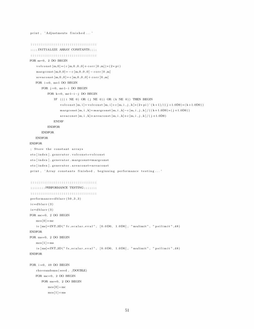
pr int , ’ Adjustments f i n i s h e d . . . ’

; ; ; ; ; ; ; ; ; ; ; ; ; ; ; ; ; ; ; ; ; ; ; ; ; ; ; ; ; ; ; ; ; ;

; ; ; ; INITIALIZE ARRAY CONSTANTS ; ; ; ;

; ; ; ; ; ; ; ; ; ; ; ; ; ; ; ; ; ; ; ; ; ; ; ; ; ; ; ; ; ; ; ; ; ;

FOR m=0, 2 DO BEGIN

vo l cons t [m,0 ]=( c [m,0 ,0 ,0 ]+ co r r [ 0 ,m] )∗ ( 2∗ pi )

margconst [m,0 ,0]=− c [m,0 ,0 ,0 ]− co r r [ 0 ,m]

areaconst [m,0 ,0 ]= c [m,0 ,0 ,0 ]+ co r r [ 0 ,m]

FOR i =0, m+1 DO BEGIN

FOR j =0, m+1− i DO BEGIN

FOR k=0, m+1−i−j DO BEGIN

IF ( ( ( i NE 0) OR ( j NE 0)) OR (k NE 0)) THEN BEGIN

vo l cons t [m, i ]= vo l cons t [m, i ]+c [m, i , j , k ]∗ (2∗ pi )ˆ ( k+1)/(( j +1.0D0)∗ ( k+1.0D0) )

margconst [m, i , k]=margconst [m, i , k]−c [m, i , j , k ] / ( ( k+1.0D0)∗ ( j +1.0D0) )

areaconst [m, i , k]= areaconst [m, i , k]+c [m, i , j , k ] / ( j +1.0D0)

ENDIF

ENDFOR

ENDFOR

ENDFOR

ENDFOR

; Store the constant ar rays

s to [ index ] . generator . vo l cons t=vo l cons t

s to [ index ] . generator . margconst=margconst

s to [ index ] . generator . a reacons t=areaconst

pr int , ’ Array constants f i n i s h ed , beg inning performance t e s t i n g . . . ’

; ; ; ; ; ; ; ; ; ; ; ; ; ; ; ; ; ; ; ; ; ; ; ; ; ; ; ; ; ; ; ; ; ;

; ; ; ; ; ; ; ; PERFORMANCE TESTING ; ; ; ; ; ; ;

; ; ; ; ; ; ; ; ; ; ; ; ; ; ; ; ; ; ; ; ; ; ; ; ; ; ; ; ; ; ; ; ; ;

performance=db la r r (50 ,3 , 3 )

i c=db la r r (3 )

i s=db la r r (3 )

FOR mc=0, 2 DO BEGIN

mcs [0 ]=mc

i c [mc]=INT 3D(” f c s c a l a r e v a l ” , [ 0 . 0D0 , 1 .0D0 ] , ”mulimit ” , ” p s i l im i t ” ,48)

ENDFOR

FOR ms=0, 2 DO BEGIN

mcs [1 ]=ms

i s [ms]=INT 3D(” f s s c a l a r e v a l ” , [ 0 . 0D0 , 1 .0D0 ] , ”mulimit ” , ” p s i l im i t ” ,48)

ENDFOR

FOR i =0, 49 DO BEGIN

rho=randomu( seed , /DOUBLE)

FOR mc=0, 2 DO BEGIN

FOR ms=0, 2 DO BEGIN

mcs [0 ]=mc

mcs [1 ]=ms

51

PROFILER, /SYSTEM

t r i a l p o i n t=po l y t r i g en ( rho )

PROFILER, DATA=preops , /REPORT

PROFILER, /SYSTEM

p=pfunc ( [ rho , t r i a l p o i n t . va lues [ 0 ] , t r i a l p o i n t . va lues [ 1 ] ] )

accept=( t r i a l p o i n t . va lues [ 2 ] LE p)

PROFILER, DATA=exeops , /REPORT

pre numops=( s i z e ( preops ) ) [ 1 ]

exe numops=( s i z e ( exeops ) ) [ 1 ]

pre =0.0D0

exe=0.0D0

FOR j =0, pre numops−1 DO pre=pre+preops [ j ] . TIME

FOR j =0, exe numops−1 DO exe=exe+exeops [ j ] . TIME

performance [ i ,mc ,ms]= i c [mc]/ (2∗ ip )∗ pre+( i c [mc]− i s [ms ] ) / ip ∗ exe

ENDFOR

ENDFOR

ENDFOR

print , ’ Performance t e s t f i n i s h e d . . . ’

; ; ; ; ; ; ; ; ; ; ; ; ; ; ; ; ; ; ; ; ; ; ; ; ; ; ; ; ; ; ; ; ; ;

; ; ;MEAN/VARIANCE OF PERFORMANCE; ; ;

; ; ; ; ; ; ; ; ; ; ; ; ; ; ; ; ; ; ; ; ; ; ; ; ; ; ; ; ; ; ; ; ; ;

per formance var=DBLARR(20)

mean=DBLARR(3 ,3 )

e r r o r=DBLARR(3 ,3 )

FOR mc=0, 2 DO BEGIN

FOR ms=0, 2 DO BEGIN

FOR i =0, 19 DO performance var [ i ]=performance [ i ,mc ,ms ]

mtmp=mean( per formance var )/ performance const mean

mean [mc,ms]=mtmp

ertmp=var iance ( per formance var )

; here we use propagat ion o f e r r o r on the quant i ty

; performance ( polynomial )/ performance ( constant )

e r r o r [mc ,ms]= sq r t ( ( ertmp/performance const mean )ˆ2+ $

( pe r f o rmance con s t e r r o r ∗mtmp/performance const mean ˆ2)ˆ2)

ENDFOR

ENDFOR

; Store the performance t e s t i n g r e s u l t s

s to [ index ] . mean=mean

sto [ index ] . e r r o r=e r r o r

pr int , ’ Setup complete f o r index : ’ , index

END

52

C.3 The SEARCHSETUP procedure: re-implementation of SETUP

PRO SEARCHSETUP, npoints , s1 , s2

; This procedure w i l l s e t up a r e j e c t i o n−with−constant t r i a l po int

; generator , and then perform a search over npo ints random po int s in

; the domain to f i nd i f there ’ s an approximation s t a r t i n g po int

; and order r e s u l t i n g in a t r i a l po int generator more e f f i c i e n t than

; the uniform t r i a l po int generator

; ; ; ; ; ; ; ; ; ; ; ; ; ; ; ; ; ; ; ; ; ; ; ; ; ; ; ; ; ; ; ; ; ;

; ; ; ; ;COMMON BLOCK DEFINITIONS ; ; ; ; ;

; ; ; ; ; ; ; ; ; ; ; ; ; ; ; ; ; ; ; ; ; ; ; ; ; ; ; ; ; ; ; ; ; ;

COMMON SCALARS, pi , param 1 , param 2

COMMON TRIGEN, setup out , p m , seed , index , mcs , cons t swi tch

COMMON BESTPOINTS, winners , b e s t i n d i c e s

COMMON INT PFUNC, ip , performance const mean , pe r f o rmance con s t e r r o r

; ; ; ; ; ; ; ; ; ; ; ; ; ; ; ; ; ; ; ; ; ; ; ; ; ; ; ; ; ; ; ; ; ;

; ; ; ; SCALAR & MISC. CONSTANTS ; ; ; ; ; ;

; ; ; ; ; ; ; ; ; ; ; ; ; ; ; ; ; ; ; ; ; ; ; ; ; ; ; ; ; ; ; ; ; ;

mcs=l indgen (2)

p i =3.14159265358979D0

param 1=s1

param 2=s2

seed=f l o o r (10∗ syst ime (/JULIAN)/ pi )

i=0

i t e r =5000

p r e c i s i o n =1.0D−6

p m=0

WHILE ( i LT 5) DO BEGIN

xmax=AMOEBA( pr e c i s i on , FUNCTION NAME=”negpfunc ” , NMAX=i t e r , $

SCALE=[5.0D−1 ,5.0D−1, p i ] , P0=[5.0D−1 ,5.0D−1, p i ] )

IF ( ( s i z e (xmax ) ) [ 0 ] EQ 0) THEN BEGIN

i++

p r e c i s i o n=p r e c i s i o n ∗10 .0D0

i t e r=i t e r +10.0D0ˆ i

ENDIF ELSE i=5

ENDWHILE

IF ( ( s i z e (xmax ) ) [ 0 ] EQ 0) THEN BEGIN

pr int , ’ Fa i l ed to f i nd maximum of func t i on with s u f f i c i e n t accuracy . ’

STOP

ENDIF ELSE BEGIN

p m=pfunc (xmax )∗ ( 1 . 0D0 + p r e c i s i o n ∗2)

ENDELSE

ip=INT 3D(” p f un c s c a l a r e v a l ” , [ 0 . 0D0 , 1 . 0D0 ] , ”mulimit ” , ” p s i l im i t ” ,96)

; data : 20 random s t a r t i n g points , choose e r r o r or mean (2 ) , 3

; p o s s i b l e o rde r s o f approxmation ( in the comparison func t i on ) , and 3

53

; p o s s i b l e o rde r s o f approximation ( in the squeeze func t i on )

s e tup cons tan t s = CREATE STRUCT( ’ c ’ , db la r r ( 3 , 4 , 4 , 4 ) , $

’ corr ’ , db la r r ( 2 , 3 ) , $

’ vo lconst ’ , db la r r ( 3 , 4 ) , $

’ margconst ’ , db la r r ( 3 , 4 , 4 ) , $

’ areaconst ’ , db la r r ( 3 , 4 , 4 ) , $

’ s ta r t ’ , db la r r ( 3 ) )

se tup out = CREATE STRUCT( ’ s t a r tpo in t ’ , [ 0 . 0D0 , 0 . 0D0 , 0 . 0D0 ] , $

’ generator ’ , s e tup cons tan t s , $

’mean ’ , db la r r ( 3 , 3 ) , ’ e r ro r ’ , db la r r ( 3 , 3 ) )

se tup out = REPLICATE( setup out , npo ints )

pr int , ’ Dec l a ra t i on s complete . . . ’

; performance t e s t i n g f o r constant , which w i l l be used as a standard

; aga in s t which a l l other gene ra to r s are compared

per formance const=db la r r (50)

FOR i =0, 49 DO BEGIN

t ime cons t =0.0D0

rho=RANDOMU( seed , /DOUBLE)

PROFILER, /SYSTEM

t r i a l p o i n t=con s t r i g en ( rho )

PROFILER, DATA=ops , /REPORT

numops=SIZE( ops )

FOR j =0, numops [1]−1 DO t ime cons t=t ime cons t+ops [ j ] . TIME

per formance const [ i ]= t ime cons t ∗pi ∗p m/ ip

ENDFOR

per f o rmance cons t e r r o r=VARIANCE( per formance const )

performance const mean=MEAN( per formance const )

pr int , ’ Performance t e s t i n g f o r uniform complete , beg inning setup at : ’ , $

npoints , ’ random po int s with in the sample space . . . ’

cons t sw i tch=0

FOR i =0, npoints−1 DO BEGIN

xrand=[RANDOMU( seed , /DOUBLE) , RANDOMU( seed , /DOUBLE) , $

2∗ pi ∗RANDOMU( seed , /DOUBLE) ]

index=i

setup , xrand

ENDFOR

print , ’ Setup complete f o r a l l po ints , beg inning search f o r minimum . . . ’

; FINALLY, the moment we ’ ve been wait ing f o r : search f o r the

; i n d i c e s conta in ing with the lowest four mean marginal execut ion t imes and s t o r e

; them f o r p l o t t i n g . For the f u l l −blown s imulat ion , only the

; ” ab so l u t e l owe s t ” and ” ab so l u t e l owe s t i nd ex ” va r i a b l e s are needed

; in order to s e t the constant s c o r r e c t l y .

; We’ l l s t a r t by f i l l i n g the minimum mean execut ion time with

; something huge ;

b ig =1.0D9

54

ind=1

; Store the winners in a s t r u c tu r e that p lo tout w i l l use :

winner=CREATE STRUCT( ’ index ’ , ind , ’ lowest ’ , b ig )

winners=REPLICATE( winner , 4 )

; Globa l ly most e f f i c i e n t o rde r s /mean m.m. e . t . ( to be changed )

ab so l u t e l owe s t i nd ex=lona r r (2 )

ab so l u t e l owe s t =1.0D9

FOR i =0, npoints−1 DO BEGIN

; Star t with something big , work our way down ;

low tmp=1.0D9

FOR mc=0, 2 DO BEGIN

FOR ms=0, 2 DO BEGIN

; I t e r a t e over each order o f approximation , f i nd the lowest mean

; marginal execut ion time

IF ( low tmp GT setup out [ i ] . mean [mc,ms ] ) THEN BEGIN

low tmp=setup out [ i ] . mean [mc,ms ]

; Hunt f o r the abso lu te most e f f i c i e n t

IF ( ab so l u t e l owe s t GE setup out [ i ] . mean [mc,ms ] ) THEN BEGIN

abso l u t e l owe s t=setup out [ i ] . mean [mc,ms ]

ab s o l u t e l owe s t i nd ex =[mc,ms ]

ENDIF

ENDIF

ENDFOR

ENDFOR

; I f there ’ s a new contender f o r lowest 4 , r ear range the array

; from g r e a t e s t to l e a s t mean marginal execut ion time , put the new low

; in , and e l im ina t e any that i t de f eated

IF ( low tmp LT winners [ 0 ] . l owest ) THEN BEGIN

pr int , ’New member o f best 4 found at index : ’ , i

winners [ 0 ] . index=i

winners [ 0 ] . l owest=low tmp

FOR j =1, 3 DO BEGIN

IF ( low tmp LT winners [ j ] . l owest ) THEN BEGIN

winners [ j −1] . index=winners [ j ] . index

winners [ j −1] . l owest=winners [ j ] . l owest

winners [ j ] . index=i

winners [ j ] . l owest=low tmp

ENDIF

ENDFOR

ENDIF

ENDFOR

be s t i n d i c e s=lona r r (4 )

FOR i =0,3 DO be s t i n d i c e s [ i ]=winners [ i ] . index

; For the s imu la t i on : s e t the index / order o f approximation to the

; optimal one that was found so that the generator uses i t . I f the re

55

; was not found any polynomial t r i a l po int gene ra to r s more e f f i c i e n t

; than the uniform t r i a l po int generator , j u s t use the uniform one .

IF ( ab so l u t e l owe s t GT performance const mean ) THEN const swi tch=1

index=be s t i n d i c e s [ 3 ]

mcs=ab so l u t e l owe s t i nd ex

pr int , ’ I n i t i a l i z a t i o n rout ine complete . Best four setup po in t s were at i n d i c e s : ’ , $

b e s t i n d i c e s

pr int , ’ Saving data . . . ’

; Put data in to f i l e s f o r p l o t t i n g :

p lotout , 0 . 5 , 1

END

C.4 Saving unformatted text data to files for plotting

PRO PLOTOUT, rho , npts , csw

; This procedure j u s t puts a l l the data in to f i l e s , to be so r t ed and

; p l o t t ed l a t e r in Mathematica ( which I ’m much more f am i l i a r with )

COMMON TRIGEN, setup out , p m , seed , index , mcs , cons t swi tch

COMMON BESTPOINTS, winners , b e s t i n d i c e s

openw , 1 , ’ out1 . dat ’

openw , 2 , ’ out2 . dat ’

openw , 3 , ’ out3 . dat ’

openw , 4 , ’ out4 . dat ’

openw , 5 , ’ r e j e c t i o n o u t . dat ’

openw , 6 , ’ s t a r t 1 . dat ’

openw , 7 , ’ s t a r t 2 . dat ’

openw , 8 , ’ s t a r t 3 . dat ’

openw , 9 , ’ s t a r t 4 . dat ’

FOR I=0, 2 DO BEGIN

FOR j =0, 2 DO BEGIN

pr in t f , 1 , s e tup out [ b e s t i n d i c e s [ 0 ] ] . mean [ i , j ] , s e tup out [ b e s t i n d i c e s [ 0 ] ] . e r r o r [ i , j ]

p r i n t f , 2 , s e tup out [ b e s t i n d i c e s [ 1 ] ] . mean [ i , j ] , s e tup out [ b e s t i n d i c e s [ 1 ] ] . e r r o r [ i , j ]

p r i n t f , 3 , s e tup out [ b e s t i n d i c e s [ 2 ] ] . mean [ i , j ] , s e tup out [ b e s t i n d i c e s [ 2 ] ] . e r r o r [ i , j ]

p r i n t f , 4 , s e tup out [ b e s t i n d i c e s [ 3 ] ] . mean [ i , j ] , s e tup out [ b e s t i n d i c e s [ 3 ] ] . e r r o r [ i , j ]

p r i n t f , 6 , s e tup out [ b e s t i n d i c e s [ 0 ] ] . s t a r t

p r i n t f , 7 , s e tup out [ b e s t i n d i c e s [ 1 ] ] . s t a r t

p r i n t f , 8 , s e tup out [ b e s t i n d i c e s [ 2 ] ] . s t a r t

p r i n t f , 9 , s e tup out [ b e s t i n d i c e s [ 3 ] ] . s t a r t

ENDFOR

ENDFOR

const swi tch=csw

rejtmp=0

56

FOR I=0, npts DO BEGIN

FOR K=0, npts DO BEGIN

rejtmp=REJECTION( rho )

FOR J=0,2 DO BEGIN

pr in t f , 5 , rejtmp [ j ]

ENDFOR

ENDFOR

ENDFOR

c lo s e , 1 , 2 , 3 , 4 , 5 , 6 , 7 , 8 , 9

END

57