Embed Size (px)
Citation preview
© 2014 OnCourse Learning. All Rights Reserved. 1
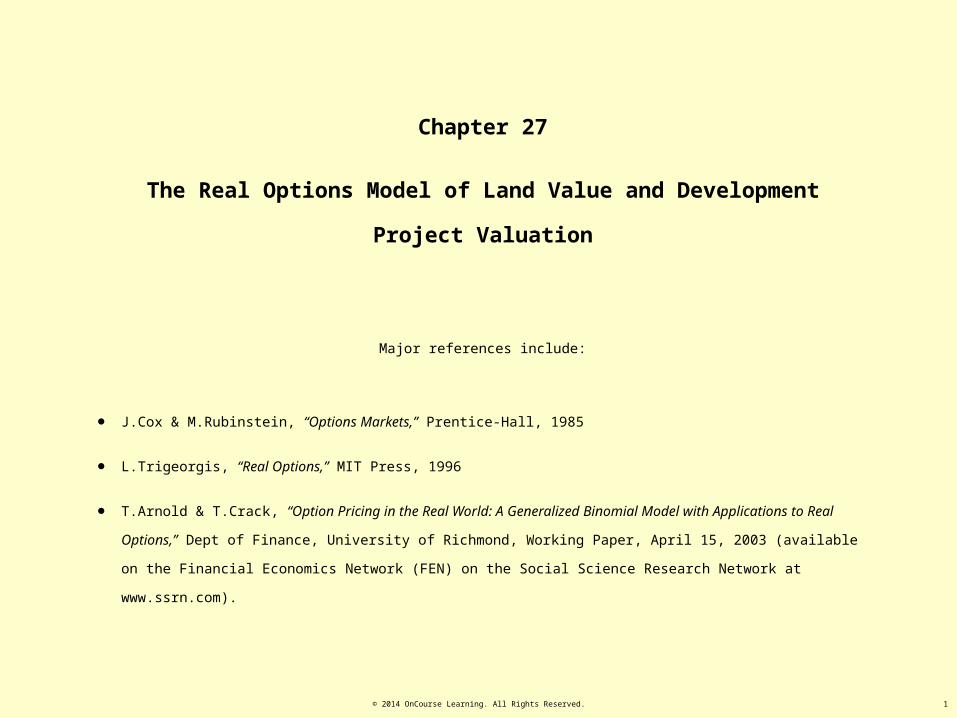
Chapter 27
The Real Options Model of Land Value and Development Project Valuation
Major references include:
• J.Cox & M.Rubinstein, “Options Markets,” Prentice-Hall, 1985
• L.Trigeorgis, “Real Options,” MIT Press, 1996
• T.Arnold & T.Crack, “Option Pricing in the Real World: A Generalized Binomial Model with Applications to Real Options,” Dept of
Finance, University of Richmond, Working Paper, April 15, 2003 (available on the Financial Economics Network (FEN) on the
Social Science Research Network at www.ssrn.com).
© 2014 OnCourse Learning. All Rights Reserved. 2
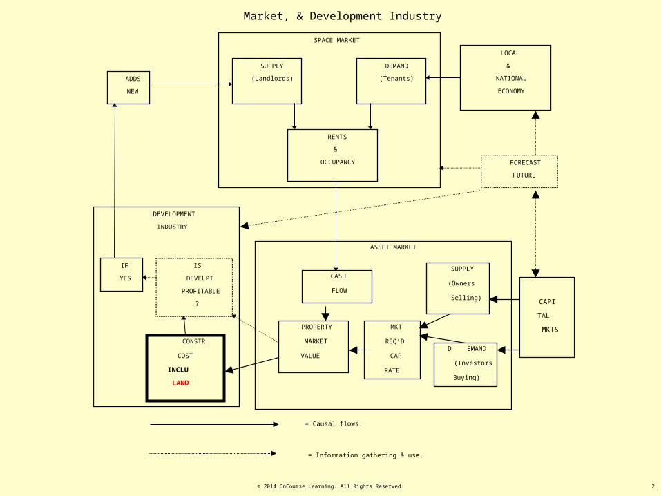
Exhibit 2-2: The “Real Estate System”: Interaction of the Space Market, Asset Market, & Development Industry SPACE MARKET
SUPPLY
(Landlords)
DEMAND
(Tenants)
RENTS
&
OCCUPANCY
LOCAL
&
NATIONAL
ECONOMY
FORECAST
FUTURE
ASSET MARKET
SUPPLY
(Owners
Selling)
D EMAND
(Investors
Buying)
CASH
FLOW
MKT
REQ’D
CAP
RATE
PROPERTY
MARKET
VALUE
DEVELOPMENT
INDUSTRY
IS
DEVELPT
PROFITABLE
?
CONSTR
COST
INCLU
LAND
IF
YES
ADDS
NEW
CAPI
TAL
MKTS
= Causal flows.
= Information gathering & use.

© 2014 OnCourse Learning. All Rights Reserved. 3
Land value plays a pivotal role in determining whether, when, and what type of development will (and
should) occur.
• From a finance/investments perspective:
- Development activity links the asset & space markets;
- Determines L.R. supply of space, L.R. rents.
- Greatly affects profitability, returns in the asset market.
• From an urban planning perspective:
- Development activity determines urban form;
- Affects physical, economic, social character of city.
Land
Value
Optimal
Devlpt
Relationship is two-way:
Recall relation of land value to land use boundaries noted in Ch.5…

© 2014 OnCourse Learning. All Rights Reserved. 4
Effect of Urban Growth & Uncertainty on Land Rents & Land Values Just Beyond the Urban Boundary
Exhibit 5-1: Components of Land Rent Outside & Inside the Urban Boundary, Under
Uncertainty . . .
Distance from CBD
B
B = Urban Boundary
Agricultural Rent
Construction Rent
Irreversibility Rent
Location Rent
Exhibit 5-2: Components of Land Value Outside & Inside the Urban Boundary, Under
Uncertainty . . .
Distance from CBD
BB = Urban Boundary
Agricultural Value
Irreversibility Premium
Construction Cost
Location Value
Growth Premium
When you develop today, you give up the option to develop
tomorrow instead. Devlpr needs to be compensated for loss of
this option.
PV of property asset includes PV of expected future growth in
rents developed property can earn after its development.

© 2014 OnCourse Learning. All Rights Reserved. 5
Effect of Urban Growth & Uncertainty on Land Rents & Land Values Just Beyond the Urban Boundary
Exhibit 5-1: Components of Land Rent Outside & Inside the Urban Boundary, Under
Uncertainty . . .
Distance from CBD
B
B = Urban Boundary
Agricultural Rent
Construction Rent
Irreversibility Rent
Location Rent
Exhibit 5-2: Components of Land Value Outside & Inside the Urban Boundary, Under
Uncertainty . . .
Distance from CBD
BB = Urban Boundary
Agricultural Value
Irreversibility Premium
Construction Cost
Location Value
Growth Premium
As boundary expands, land value just beyond
boundary can grow rapidly, due to increase in
growth premium & irreversibility (option)
premium values, depending on how fast the
boundary is expanding, the magnitude of the
location value rent gradient inside the boundary,
and the magnitude of uncertainty (volatility) in
that growth.
Direction of bdy expansion
Direction of time flow

© 2014 OnCourse Learning. All Rights Reserved. 6
Different conceptions of “land value” (Recall Property Life Cycle theory from Ch.5)
Property Value, Location Value, & Land Value
Evolution of the Value (& components) of a Fixed Site (parcel)
0.0
0.5
1.0
1.5
2.0
2.5
3.0
C C C C
Time ("C" Indicates Reconstruction times)
Val
ue L
evel
s ($
)
HBU Value As IfVacant = PotentialUsage Value, or"Location Value"("U")
Property Value("P") = Mkt Val(MV) = StructureValue + LandValue.
Land Value byLegal/AppraisalDefn. ("land compsMV").
Land Value byEcon.Defn. =Redevlpt OptionValue. ("LAND")
In Ch.27 we focus on the
Econ.Defn.: “LAND”

© 2014 OnCourse Learning. All Rights Reserved. 7
Different conceptions of “land value”
Property Value, Location Value, & Land Value
Evolution of the Value (& components) of a Fixed Site (parcel)
0.0
0.5
1.0
1.5
2.0
2.5
3.0
C C C C
Time ("C" Indicates Reconstruction times)
Val
ue L
evel
s ($
)
HBU Value As IfVacant = PotentialUsage Value, or"Location Value"("U")
Property Value("P") = Mkt Val(MV) = StructureValue + LandValue.
Land Value byLegal/AppraisalDefn. ("land compsMV").
Land Value byEcon.Defn. =Redevlpt OptionValue. ("LAND")
Note that there are points
in time when three of the
four definitions all give the
same value, namely,
property value = land value
defined by either defn at
the times of optimal
redevelopment
(construction) on the site.

© 2014 OnCourse Learning. All Rights Reserved. 8
The economic definition of land value (“LAND”) is based on nothing more or less than the fundamental
capability that land ownership gives to the landowner (unencumbered):
The right without obligation to develop (or redevelop) the property.

© 2014 OnCourse Learning. All Rights Reserved. 9
Evolution of the Value (& components) of a Fixed Site (parcel)
0.0
0.5
1.0
1.5
2.0
2.5
3.0
C C C CTime ("C" Indicates Reconstruction times)
Va
lue
Le
vels
($
)
This definition of land value is most relevant
Just prior to the times when development or redevelopment occurs on the site.

© 2014 OnCourse Learning. All Rights Reserved. 10
To understand the economic conception of land value, a famous theoretical development from
financial economics is most useful: “Option Valuation Theory” (OVT) :
In particular, a branch of that theory known a “Real Options.”
© 2014 OnCourse Learning. All Rights Reserved. 11
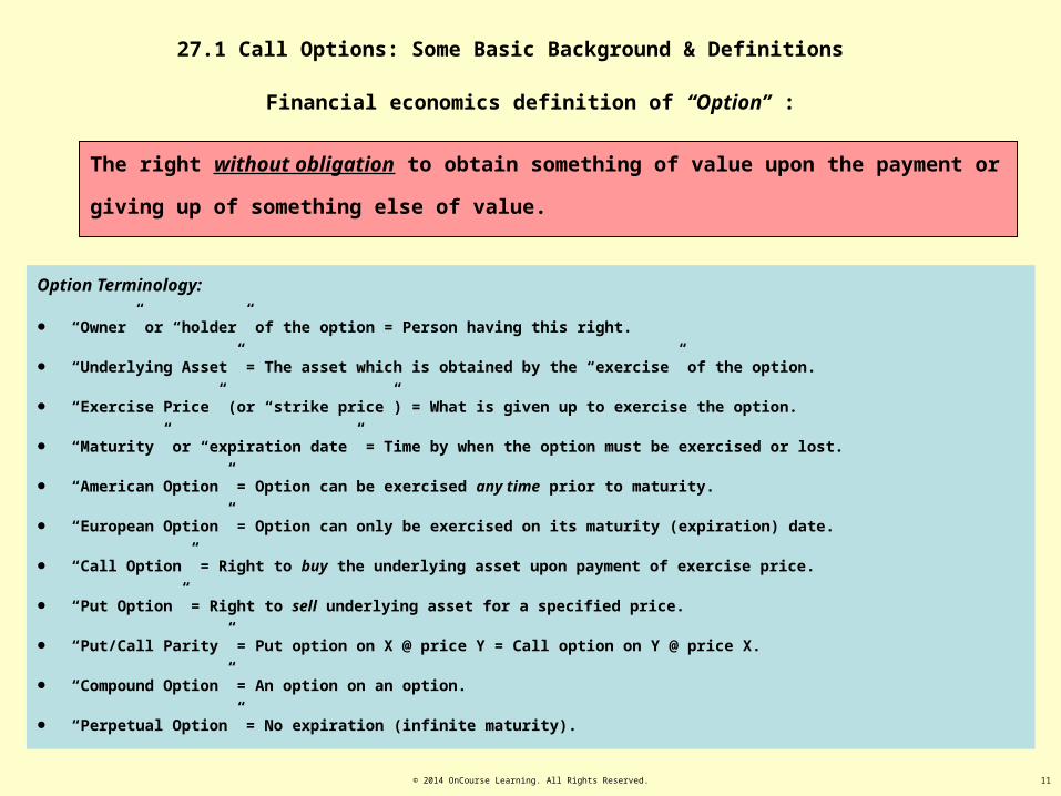
27.1 Call Options: Some Basic Background & Definitions
The right without obligation to obtain something of value upon the payment or giving up of something
else of value.
Financial economics definition of “Option” :
Option Terminology:
• “Owner” or “holder” of the option = Person having this right.
• “Underlying Asset” = The asset which is obtained by the “exercise” of the option.
• “Exercise Price” (or “strike price”) = What is given up to exercise the option.
• “Maturity” or “expiration date” = Time by when the option must be exercised or lost.
• “American Option” = Option can be exercised any time prior to maturity.
• “European Option” = Option can only be exercised on its maturity (expiration) date.
• “Call Option” = Right to buy the underlying asset upon payment of exercise price.
• “Put Option” = Right to sell underlying asset for a specified price.
• “Put/Call Parity” = Put option on X @ price Y = Call option on Y @ price X.
• “Compound Option” = An option on an option.
• “Perpetual Option” = No expiration (infinite maturity).

© 2014 OnCourse Learning. All Rights Reserved. 12
Option exercise is irreversible:
Options can only be exercised once. Then the option is lost.
OVT is a body of theory and methodology for quantitatively evaluating options.
• For American options, this includes the problem of specifying the conditions when it is optimal to
exercise the option: Optimal Exercise Policy.
• For the land development option, this relates to the conditions when it is optimal to develop (or redevelop) the
land.

© 2014 OnCourse Learning. All Rights Reserved. 13
Some history:
Call option model of land arose from two strands of theory:
• Financial economics study of corporate capital budgeting,
• Urban economics study of urban spatial form.
Capital Budgeting:
• How corporations should make capital investment decisions (constructing physical plant, long-lived
productive assets).
• Includes question of optimal timing of investment.
• e.g., McDonald, Siegel, Myers, (others), 1970s-80s.
Urban Economics:
• What determines density and rate of urban development.
• Titman, Williams, Capozza, (others), 1980s.
It turned out the 1965 Samuelson-McKean Model of a perpetual American warrant was the essence of what they
were all using.

© 2014 OnCourse Learning. All Rights Reserved. 14
The value of newly-built property will include the (remaining) economic value of the land (“LAND”), but:
• This land value will now be minus its initial development option value (which has been exercised),
• It will include the redevelopment (or abandonment) option value.
• However, this redevelopment option value will normally be quite small in a newly developed property
(recall property “life-cycle” chart).
Evolution of the Value (& components) of a Fixed Site (parcel)
0.0
0.5
1.0
1.5
2.0
2.5
3.0
C C C CTime ("C" Indicates Reconstruction times)
Va
lue
Le
vels
($
)
Speaking in terms of the
economic definition of land
value, based on its option
value.

© 2014 OnCourse Learning. All Rights Reserved. 15
The Land Development Option Contrasted with Financial Options:
Distinguishing characteristics of the land devlpt option:
• Perpetual (no expiriation):
• More flexibility (greater value),
• Only reason to exercise is to obtain operating cash flows.
• “Time to Build” (exercise not immediate):
• Can’t observe exact at-completion mkt val of underl.asset at time exercise decision is made (added risk in exercise decision).
• “Noisy” value observation of (even current) mkt val of underl. asset. (“thin mkt”, recall Ch.12, also adds to risk of exercise
decision):
• Possibly heterogeneous information about true value of underlying asset (the to-be-built property): Some devlprs may be more
knowledgable than others. ( Wait longer until exercise.)
• Exercise creates new real assets that add to the supply side of the space market (affecting mkt val of all competing
properties):
• Can increase risk of not exercising (option may effectively “expire” if demand is absorbed by competing devlpt projects).

© 2014 OnCourse Learning. All Rights Reserved. 16
What the real option theory of land development can tell us about the “overbuilding phenomenon”
What is the “overbuilding phenomenon”?
The widely observed tendency for commercial real estate markets to periodically become “overbuilt”,
that is, characterized by excess supply (abnormally high vacancy, downward pressure on rents), due to
excessive speculative development of new buildings.
Recall that in Chapter 2 we discussed an explanation for this “cyclicality” phenomenon using the “4-
Quadrant Diagram”, based on the existence of myopic behavior (not just lack of perfect foresight, but some
degree of irrational expectations) on the part of investors and developers in the system .

17
Rent $
Stock (SF)Price $
Construction (SF)
Space Market:
Stock Adjustment
Asset Market:
Construction
Space Market:
Rent DeterminationAsset Market:
Valuation
Q*
R*
P*
C*
D0
D1
Exhibit 2-4a: Effect of Demand Growth in Space Market:
© 2
014
OnC
ours
e Le
arni
ng. A
ll Ri
ghts
Res
erve
d.

18
Rent $
Stock (SF)Price $
Construction (SF)
Space Market:
Stock Adjustment
Asset Market:
Construction
Space Market:
Rent DeterminationAsset Market:
Valuation
Q*
R*
P*
C*
D0
D1
R1
P1
Exhibit 2-4a: Effect of Demand Growth in Space Market: First phase…
Can this be a long-run equilibrium
result?…
Doesn’t form a rectangle.
© 2
014
OnC
ours
e Le
arni
ng. A
ll Ri
ghts
Res
erve
d.

© 2014 OnCourse Learning. All Rights Reserved. 19
Rent $
Stock (SF)Price $
Construction (SF)
Space Market:
Stock Adjustment
Asset Market:
Construction
Space Market:
Rent DeterminationAsset Market:
Valuation
Q*
R*
P*
C*
D0
D1
R1
P1
Exhibit 2-4a: Effect of Demand Growth in Space Market: LR Equilibrium…
R**
P**
C**
Q**

© 2014 OnCourse Learning. All Rights Reserved. 20
Real option theory offers several explanations for why/how overbuilding can be due to completely rational
(i.e., profit-maximizing) behavior on the part of developers (landowners):
1. “Cascades”: Noisy observations of the mkt values of the underlying assets (comparable built properties), combined with
heterogeneous developer knowledge about the “true” value, causes a follow-the-leader type effect, in which developers wait
longer than they otherwise would to develop, and then they all rush in as soon as the first (presumably most knowledgeable)
developer reveals his knowledge by commencing development.
2. “Lumpy supply & first out of the gate”: Economies of scale in building size, combined with finite user demand and the fact that
option exercise creates real physical capital, leads to early exercise of the development option to preclude loss (expiration) of the
option if a competitor builds first.
3. “Long-term leasing option”: The cost of having empty space in a new building may be less than it first appears in space markets
characterized by long-term leases, as it gives the landlord a leasing option, that has value prior to its “exercise” (in the signing of a
lease contract): Volatility in the rental mkt may bring better long-term lease deals in the future.

© 2014 OnCourse Learning. All Rights Reserved. 21
Chapter 27: Real Options & Land Value
Options whose underlying assets (either what is obtained or what is given up on the exercise of the option) are
real assets (i.e., physical capital).
Real Options:
The call option model of land value (introduced in Chapter 5) is a real option model:
Land ownership gives the owner the right without obligation to develop (or redevelop) the property upon payment of the
construction cost. Built property is underlying asset, construction cost is exercise price (including the opportunity cost of the loss of
any pre-existing structure that must be torn down).
In essence, all real estate development projects are real options, though in some simple cases the optionality may
be fairly trivial and can be safely ignored.

© 2014 OnCourse Learning. All Rights Reserved. 22
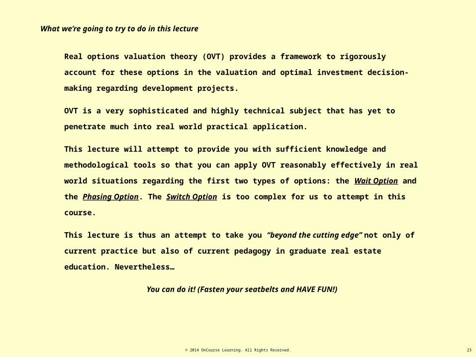
What we’re going to try to do in these lectures
In the typical development project (or parcel of developable land), there are three major types of options
that may present themselves:*
• “Wait Option”: The option to delay start of the project construction (Ch.27);
• “Phasing Option”: The breaking of the project into sequential phases rather than building it all at
once (Ch.29);
• “Switch Option”: The option to choose among alternative types of buildings to construct on the given
land parcel.
All three of these types of options can affect optimal investment decision-making, add significantly to the
value of the project (and of the land), affect the risk and return characteristics of the investment, and they
are difficult to accurately account for in traditional DCF investment analysis.
© 2014 OnCourse Learning. All Rights Reserved. 23
What we’re going to try to do in this lecture
Real options valuation theory (OVT) provides a framework to rigorously account for these options in the
valuation and optimal investment decision-making regarding development projects.
OVT is a very sophisticated and highly technical subject that has yet to penetrate much into real world
practical application.
This lecture will attempt to provide you with sufficient knowledge and methodological tools so that you can
apply OVT reasonably effectively in real world situations regarding the first two types of options: the Wait
Option and the Phasing Option. The Switch Option is too complex for us to attempt in this course.
This lecture is thus an attempt to take you “beyond the cutting edge” not only of current practice but also of
current pedagogy in graduate real estate education. Nevertheless…
You can do it! (Fasten your seatbelts and HAVE FUN!)

© 2014 OnCourse Learning. All Rights Reserved. 24
What we’re going to try to do in this lecture
We will begin by considering the Wait Option, which is the simplest of the three types of options . . .

© 2014 OnCourse Learning. All Rights Reserved. 25
Today Next Year
Probability 100% 30% 70%
Value of Developed Property $100.00 $78.62 $113.21
Development Cost (exclu land) $88.24 $90.00 $90.00
NPV of exercise $11.76 -$11.38 $23.21
(Action) (Don’t build) (Build)
Future Values 0 $23.21
Expected Values $11.76 $16.25
= Sum[ Probability X Outcome ] (1.0)11.76 (0.3)0 + (0.7)23.21
PV(today) of Alternatives @20% $11.76 16.25 / 1.2 = $13.54Note: In this example the expected growth in the HBU value of the built property is 2.83%: as (.3)78.62 + (.7)113.21 = $102.83.
What is the value of this land today? Answer: = MAX[11.76, 13.54] = $13.54
Should owner build now or wait? Answer: = Wait. (100.00 – 88.24 – 13.54< 0.)
The $13.54 – $11.76 = $1.78 option premium is due to uncertainty or volatility.
27.2 A Simple Numerical Example of OVT Applied to Land Valuation and the Development Timing Decision

© 2014 OnCourse Learning. All Rights Reserved. 26
Note the importance of flexibility inherent in the option (“right without obligation”), which allows the negative downside outcome to
be avoided. This gives the option a positive value and results in the “irreversibility premium” in the land value (noted in Geltner-
Miller Ch.5).
Consider the effect of uncertainty (or volatility) in the evolution of the built property value (for whatever building would be built on
the site), and the fact that development at any given time is mutually exclusive with development at any other time on the same site
(“irreversibility”). e.g.:
Today Next Year
Probability 100% 30% 70%
Value of Developed Property $100.00 $78.62 $113.21
Development Cost (exclu land) $88.24 $90.00 $90.00
NPV of exercise $11.76 -$11.38 $23.21
(Action) (Don’t build) (Build)
Future Values 0 $23.21
Expected Values $11.76 $16.25
= Sum[ Probability X Outcome ] (1.0)11.76 (0.3)0 + (0.7)23.21
PV(today) of Alternatives @20% $11.76 16.25 / 1.2 = $13.54

© 2014 OnCourse Learning. All Rights Reserved. 27
Representation of the preceding problem as a “decision tree”:
Build: Get
113.21-90.00
= $23.21
70%
30%
Don’t build:
Get 0.
• Identify decisions and alternatives (nodes & branches).
• Assign probabilities (sum across all branches @ ea. node = 100%).
• Locate nodes in time.
• Assume “rational” (highest value) decision will be made at each node.
• Discount node expected values (means) across time reflecting risk.
Choice Next Yr.:
Node Value = (7.)23.21+ (.3)0 =
$16.25.
1 Yr
Wait Today:
PV = 16.25/1.2 = 13.54.
Build Today:
Get 100.00-88.24 =
$11.76.
Choice
Today
Decision Tree Analysis is closely related to Option Valuation Methodology, but
requires a different type of simplification (finite number of discrete alternatives).

© 2014 OnCourse Learning. All Rights Reserved. 28
A problem with traditional decision tree analysis
1 Yr
Choice
Today
But is this really the correct discount rate (and hence, the correct
decision and valuation of the project)?...
Build: Get
113.21-90.00
= $23.21
70%
30%
Don’t build:
Get 0.
Choice Next Yr.:
Node Value = (7.)23.21+ (.3)0 =
$16.25.
Wait Today:
PV = 16.25/1.2 = 13.54.
Build Today:
Get 100.00-88.24 =
$11.76.
We were only able to completely evaluate this decision because we somehow knew what we thought to be the
appropriate risk-adjusted discount rate to apply to it (here assumed to be 20%).
© 2014 OnCourse Learning. All Rights Reserved. 29
Where did the 20% discount rate (OCC) come from anyway?
1 Yr
Choice
Today
To be honest…
It was a nice round number that seemed “in the ballpark” for required returns on development investment
projects.
Can we be a bit more “scientific” or rigorous? . . .
Build: Get
113.21-90.00
= $23.21
70%
30%
Don’t build:
Get 0.
Choice Next Yr.:
Node Value = (7.)23.21+ (.3)0 =
$16.25.
Build Today:
Get 100.00-88.24 =
$11.76.
Wait Today:
PV = 16.25/1.2 = 13.54.

© 2014 OnCourse Learning. All Rights Reserved. 30
Suppose there were “complete markets” in land, and buildings, and bonds, such that we could buy or sell (short if necessary)
infinitely divisible quantities of each, including land and buildings like our subject development project.
Thus, we could buy today:
• 0.67 units of a building just like the one our subject development would produce next year that will either be worth $113.21
or $78.62 then.
And we could partially finance this purchase by issuing:
• $51.21 worth of riskless bonds (with a 3% interest rate).
Then this “replicating portfolio” (long in the bldg, short in the bond) next year will be worth:
• In the “up” scenario: (0.67)$113.21 - $51.21(1.03) = $75.95 – $52.74 = $23.21, or:
• In the “down” scenario: (0.67)$78.62 - $ 51.21(1.03) = $52.74 – $52.74 = 0.
Exactly Equal to the Development Project in All Future Scenarios!
27.3.1. The Essence of Option Valuation Theory

© 2014 OnCourse Learning. All Rights Reserved. 31
Recall:
These are the future scenarios, describing all possible future outcomes.
In the upside outcome, the project will be worth $23.21,
same as the replicating portfolio.
In the downside outcome, the project will be worth 0, same
as the replicating portfolio.
1 Yr
Choice
Today
The Essence of OVT
Build: Get
113.21-90.00
= $23.21
70%
30%
Don’t build:
Get 0.
Choice Next Yr.:
Node Value = (7.)23.21+ (.3)0 =
$16.25.
Build Today:
Get 100.00-88.24 =
$11.76.
Wait Today:
PV = 16.25/1.2 = 13.54.

© 2014 OnCourse Learning. All Rights Reserved. 32
Thus, this “replicating portfolio” must be worth the same as the land (the development option) today.
Suppose not:
• If the land can be bought for less than the replicating portfolio, then I can sell the replicating portfolio short, buy the
land, pocket the difference as profit today, and have zero net value impact next year (as the land and replicating
portfolio will in all cases be worth the same next year, so my long position offsets my short position exactly).
• If the land costs more than the replicating portfolio, then I can sell the land short, buy the replicating portfolio,
pocket the difference as profit today, and once again have zero net impact next year.
This is what is known as an “arbitrage” – riskless profit!
In equilibrium (within and across markets), arbitrage opportunities cannot exist, for they would be bid away by
competing market participants seeking to earn super-normal profits.
The Essence of OVT
© 2014 OnCourse Learning. All Rights Reserved. 33
In real estate, markets are not so perfect and complete to enable actual construction of technical arbitrage. But
nevertheless competition tends to eliminate super-normal profit, so we can use this kind of analysis to model prices and
values.
Fundamentally, this approach will always equalize the expected return risk premium per unit of risk, across the asset
markets.
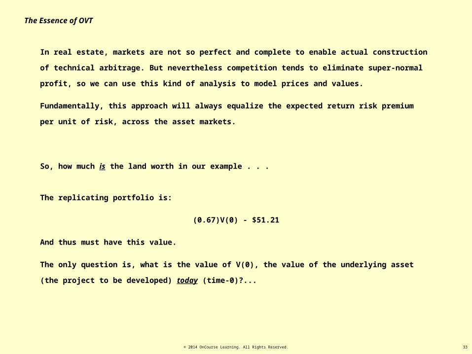
So, how much is the land worth in our example . . .
The replicating portfolio is:
(0.67)V(0) - $51.21
And thus must have this value.
The only question is, what is the value of V(0), the value of the underlying asset (the project to be developed) today (time-
0)?...
The Essence of OVT

© 2014 OnCourse Learning. All Rights Reserved. 34
We know that a similar asset already completed today is worth $100.00.
However, this value includes the value of the net cash flow (dividends, rents) that asset will pay between today and next year.
Our development project won’t produce those dividends, because it won’t produce a building until next year.
So, we need a little more analysis…
Suppose that the underlying asset (the built property) has an expected total return of 9%.
If a similar building has a value today of $100.00, and an (ex dividend) value next year of either $113.21 (70% chance) or
$78.62 (30% chance), then the expected value next year is (0.7)113.21+(0.3)78.62 = $102.83 (i.e., expected growth is
E[gV
]=2.83%).
Thus, the PV today of a building that would not exist until next year (i.e., PV of similar pre-existing building net of its cash
flow between now and next year) is:
PV[V1
] = V(0) = $102.83 / 1.09 = $94.34.
(versus V0
= $100.00 for pre-existing bldg.)
The Essence of OVT
© 2014 OnCourse Learning. All Rights Reserved. 35
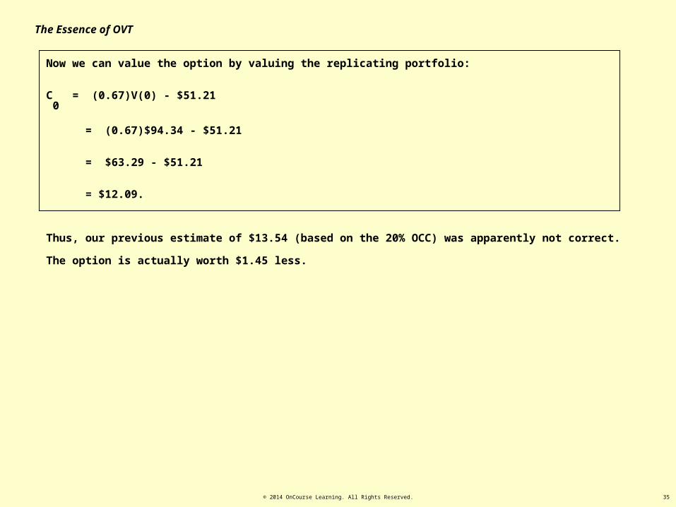
Now we can value the option by valuing the replicating portfolio:
C0
= (0.67)V(0) - $51.21
= (0.67)$94.34 - $51.21
= $63.29 - $51.21
= $12.09.
Thus, our previous estimate of $13.54 (based on the 20% OCC) was apparently not correct. The option is actually worth
$1.45 less.
The Essence of OVT
© 2014 OnCourse Learning. All Rights Reserved. 36
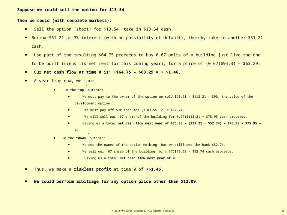
Suppose we could sell the option for $13.54
Then we could (with complete markets):
• Sell the option (short) for $13.54, take in $13.54 cash.
• Borrow $51.21 at 3% interest (with no possibility of default), thereby take in another $51.21 cash.
• Use part of the resulting $64.75 proceeds to buy 0.67 units of a building just like the one to be built (minus its net rent for this coming
year), for a price of (0.67)$94.34 = $63.29.
• Our net cash flow at time 0 is: +$64.75 – $63.29 = + $1.46.
• A year from now, we face:
• In the “up” outcome:
• We must pay to the owner of the option we sold $23.21 = $113.21 - $90, the value of the development option.
• We must pay off our loan for (1.03)$51.21 = $52.74.
• We will sell our .67 share of the building for (.67)$113.21 = $75.95 cash proceeds.
• Giving us a total net cash flow next year of $75.95 – ($23.21 + $52.74) = $75.95 - $75.95 = 0.
• In the “down” outcome:
• We owe the owner of the option nothing, but we still owe the bank $52.74.
• We sell our .67 share of the building for (.67)$78.62 = $52.74 cash proceeds.
• Giving us a total net cash flow next year of 0.
• Thus, we make a riskless profit at time 0 of +$1.46.
• We could perform arbitrage for any option price other than $12.09.

© 2014 OnCourse Learning. All Rights Reserved. 37
Today Next Year
Development Option ValueC = Max[0,V-K]
PV[C1] = x
“x” = unknown value, x = P0 , otherwise arbitrage..
C1up =113.21-90
= $23.21
C1down = 0
(Don’t build)
Built Property Value PV[V1] = E[V1] / (1+OCC)
= [(.7)113.21+(.3)78.62]/1.09 = $102.83/1.09 =$94.34
V1up = $113.21 V1
down = $78.62
Bond Value B = $51.21 B1 = (1+rf )B = (1.03)51.21
= $52.74
B1 = (1+rf )B = (1.03)51.21
= $52.74
Replicating Portfolio:P = (N)V – B
P0 = (N) PV[V1] – B
= (0.67)$94.34 - $51.21 = $63.29 - $51.21 = $12.09
P1up =(0.67)113.21 -
$52.74= $75.95 - $$52.74
= $23.21
P1down =(0.67)78.62 -
$52.74= $52.74 - $52.74
= $0
Here is another way of depicting what we have just suggested:
The replicating portfolio duplicates the option value in all future scenarios, hence its present value must be the same as the option’s present
value: C0
.
Thus, the option is worth $12.09.
27.3.1: The Arbitrage Perspective on the Option Value…
© 2014 OnCourse Learning. All Rights Reserved. 38
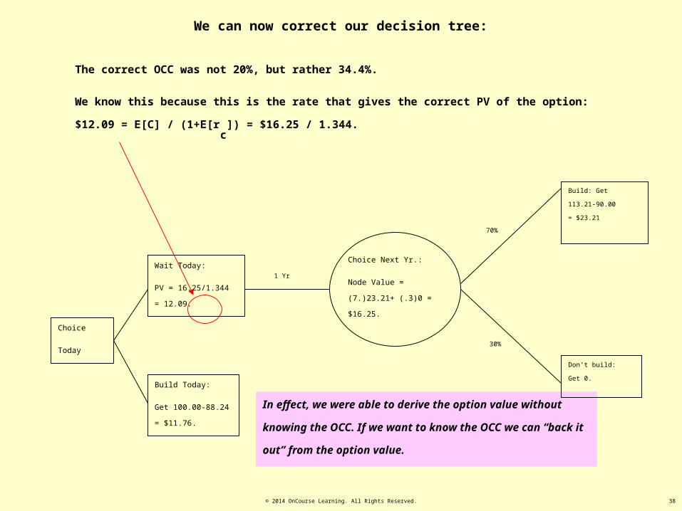
We can now correct our decision tree:
1 Yr
Choice
Today
The correct OCC was not 20%, but rather 34.4%.
We know this because this is the rate that gives the correct PV of the option: $12.09 = E[C] / (1+E[rc]) = $16.25 /
1.344.
In effect, we were able to derive the option value without knowing the
OCC. If we want to know the OCC we can “back it out” from the option
value.
Build: Get
113.21-90.00
= $23.21
70%
30%
Don’t build:
Get 0.
Choice Next Yr.:
Node Value = (7.)23.21+ (.3)0 =
$16.25.
Build Today:
Get 100.00-88.24 =
$11.76.
Wait Today:
PV = 16.25/1.344 = 12.09.

© 2014 OnCourse Learning. All Rights Reserved. 39
TD
TT
V
TT
C
TTT
rE
L
rE
V
rE
LVCPV
][1][1][1][
Note:
This options-based derivation of the OCC of developable land is completely consistent with Chapter 29’s formula for
development project OCC:
Only in the circumstance where the option will definitely be developed next period (e.g., in the previous example, if the
construction cost were $78.62 million instead of $90 million, the option would be worth $18.01 million and it would be
“ripe” for immediate development):
In all cases, the result is to provide the same expected return risk premium per unit of risk across all the asset markets (land,
buildings, bonds): the equilibrium condition within and across the relevant markets.
03.1
62.78$
09.1
83.102$
344.1
62.7883.102$01.18$

© 2014 OnCourse Learning. All Rights Reserved. 40
Here is the corrected summary of the analysis of the development project:
The land is worth: MAX[$100.00 – $88.24, C0
] = $12.09:
34.4% OCC for the option
What is the value of this land today? Answer: = MAX[11.76, 12.09] = $12.09
Should owner build now or wait? Answer: = Wait. (100.00 – 88.24 – 12.09 < 0.)
Today Next Year
Probability 100% 30% 70%
Value of Developed Property $100.00 $78.62 $113.21
Development Cost (exclu land) $88.24 $90.00 $90.00
NPV of exercise $11.76 -$11.38 $23.21
(Action) (Don’t build) (Build)
Future Values 0 $23.21
Expected Values $11.76 $16.25
= Sum[ Probability X Outcome ] (1.0)11.76 (0.3)0 + (0.7)23.21
PV(today) of Alternatives @ 34% $11.76 16.25 / 1.344 = $12.09

© 2014 OnCourse Learning. All Rights Reserved. 41
The general formula for the Replicating Portfolio in a Binomial World is:
Replicating Portfolio = NV-B, where:
“N” is “shares” (proportional value) of the underlying asset (built property) to purchase,
“B” is current (time 0) dollar value of bond to issue (borrow), and:
N=(Cu-Cd)/(Vu-Vd); and
B=(NVd-Cd)/(1+rf).
With: Cu = MAX[Vu-K, 0]; Cd = MAX[Vd-K, 0];
Vu, Vd, = “up” & “down” values of property to be built; K = constr cost.
In the preceding example:
N = (23.21-0)/(113.21-78.62) = 23.21/34.59 = 0.67; and
B = (0.67(78.62)-0)/1.03 = $52.74/1.03 = $51.21.
© 2014 OnCourse Learning. All Rights Reserved. 42
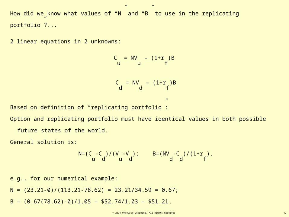
How did we know what values of “N” and “B” to use in the replicating portfolio”?...
2 linear equations in 2 unknowns:
Cu
= NVu
– (1+rf)B
Cd
= NVd
– (1+rf)B
Based on definition of “replicating portfolio”:
Option and replicating portfolio must have identical values in both possible future states of the world.
General solution is:
N=(Cu
-Cd
)/(Vu
-Vd
); B=(NVd
-Cd
)/(1+rf).
e.g., for our numerical example:
N = (23.21-0)/(113.21-78.62) = 23.21/34.59 = 0.67;
B = (0.67(78.62)-0)/1.05 = $52.74/1.03 = $51.21.

© 2014 OnCourse Learning. All Rights Reserved. 43
General solution is:
N=(Cu
-Cd
)/(Vu
-Vd
); B=(NVd
-Cd
)/(1+rf).
Combining these formulas with the definition of the replicating portfolio, we can expand the binomial option
value as:
C = NV – B
"",1,1)1(
11
11
1)0(
)0(11
)0(
)0(1
)1()1/()0(
)0(/1
)1/()0(
)0(/1
)1()0(
)0(/)1(1
)0(
)0(/)1(1
)1(
)1(
)0(
)1(
)0(
)1()1(
)()0(
1)0(
probneutralriskpdudrpwhererCppCC
rCdu
drC
du
drC
rCVVV
VVrC
VVV
VVrC
r
CC
rVVV
VVrC
rVVV
VVrC
r
CC
VVV
VrVC
VVV
VrVC
r
CC
VV
rV
VVV
CC
VV
rV
VVV
CC
r
CrV
VV
CCV
VV
CCC
rCVVV
CCV
VV
CCC
ffdu
fdf
uf
fddu
dfu
du
df
f
dd
fdu
dfu
fdu
df
f
dd
du
fdu
du
fd
f
dd
du
fd
du
du
du
fd
du
u
f
dfd
du
du
du
du
fdddu
du
du
du
Hence, the classical (Cox-Roll-
Ross) binomial option value
formula using “risk-neutral
probabilities”…

© 2014 OnCourse Learning. All Rights Reserved. 44
The previously described option valuation of a development project is completely consistent with the “Certainty Equivalent
Valuation” form of the DCF valuation model presented earlier in the Chapter 10 lecture in this course.
The general 1-period Certainty Equivalent Valuation Formula is:
09.12$03.1
45.12$
03.1
80.3$25.16$03.1
1636.021.23$25.16$
03.1
21.23$25.16$
05.1%33.83%120
%621.23$25.16$
%31
)%34.94/62.78()%34.94/21.113(
%3%90$21.23$0)$3(.21.23)$7(.
:.,.
1
%%
][][
1
][
%67.36%6
0
10
100
C
exampleouringe
r
VV
rrECCCE
r
CCEQC
f
downup
fVdownup
f
27.3.2: The Certainty-Equivalence Perspective on the Option Value…

© 2014 OnCourse Learning. All Rights Reserved. 45
I’m hoping you developed some intuition for the certainty equivalence valuation model back in Chapter 10 (CD Appendix 10C). But in case not, let’s
try this . . .
The certainty equivalent value next year is the downward adjusted value of the risky expected value for which the investment market would be
indifferent between that value and a riskfree bond value of the same amount…
f
downup
fVdownup
f r
VV
rrECCCE
r
CCEQC
1
%%
][][
1
][10
100
The certainty equivalent value next year is the expected value minus a risk discount.
%%
][
downup
fVdownup VV
rrECC
The risk discount consists of the amount of risk in the next year’s value as
indicated by the range in the possible outcomes times…
times the market price of risk.
%%
][
downup
fV
VV
rrE
The market price of risk is the market expected return risk premium per unit of return risk, the ratio of…
the market expected return risk premium divided by
the range in the corresponding return possible
outcomes.

© 2014 OnCourse Learning. All Rights Reserved. 46
Thus, we can derive the same present value of the option through two completely
consistent (mathematically equivalent) approaches:
• The “arbitrage analysis” based on the replicating portfolio, or;
• The CEQ DCF PV model.
The latter is more convenient for computations.
These two approaches are equivalent, but can be derived independently (recall that we
did NOT employ an arbitrage analysis to derive the CEQ valuation model).
This makes the valuation model very robust.

© 2014 OnCourse Learning. All Rights Reserved. 47
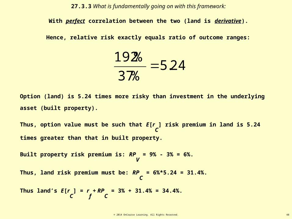
27.3.3 What is fundamentally going on with this framework:
PV[V1
]
=$94.34
V1
up=
$113.21
V1
down=
$78.62
p = 0.7
1-p = 0.3
Underlying asset (built property)
outcome % range:
%3734.94$
62.78$21.113$
PV[C1
]
=$12.09
C1
up=
$23.21
C1
down=
$0
p = 0.7
1-p = 0.3
Option (land) outcome % range:
%19209.12$
0$21.23$
With perfect correlation between the two (land is derivative).
© 2014 OnCourse Learning. All Rights Reserved. 48
27.3.3 What is fundamentally going on with this framework:
With perfect correlation between the two (land is derivative).
Hence, relative risk exactly equals ratio of outcome ranges:
24.5%37
%192
Option (land) is 5.24 times more risky than investment in the underlying asset (built property).
Thus, option value must be such that E[rC
] risk premium in land is 5.24 times greater than that in built
property.
Built property risk premium is: RPV
= 9% - 3% = 6%.
Thus, land risk premium must be: RPC
= 6%*5.24 = 31.4%.
Thus land’s E[rC
] = rf + RP
C = 3% + 31.4% = 34.4%.

© 2014 OnCourse Learning. All Rights Reserved. 49
Risk
E[r]
rf = 3.0%
34.4%
9.0%
Built Property
37% range
Devlpt Option
192% range
E[RP]
If this relationship does not hold, then there are “super-normal” (disequilibrium) profits (expected returns) to be made somewhere, and
correspondingly “sub-normal” profits elsewhere, across the markets for: Land, Stabilized Property, and Bonds (“riskless” CFs).
27.3.3 What is fundamentally going on with this framework:
The “price of risk” (the ex ante investment return risk premium per unit of risk) is being equated across the markets for land and
built property:
Exh.27-4
© 2014 OnCourse Learning. All Rights Reserved. 50
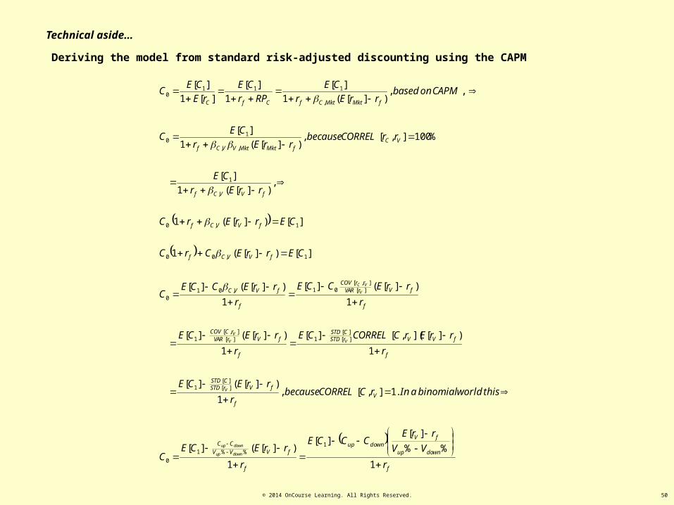
Deriving the model from standard risk-adjusted discounting using the CAPM
f
downup
fVdownup
f
fVVV
CC
Vf
fVrSTDCSTD
f
fVVrSTDCSTD
f
fVrVARrCCOV
f
fVrVARrrCOV
f
fVVC
fVVCf
fVVCf
fVVCf
VCfMktMktVVCf
fMktMktCfCfC
r
VV
rrECCCE
r
rrECEC
thisworldbinomialaInrCCORRELbecauser
rrECE
r
rrErCCORRELCE
r
rrECE
r
rrECCE
r
rrECCEC
CErrECrC
CErrErC
rrEr
CE
rrCORRELbecauserrEr
CEC
CAPMonbasedrrEr
CE
RPr
CE
rE
CEC
downup
downup
V
VV
V
V
VC
1
%%
][][
1
)][(][
.1],[,1
)][(][
1
)][](,[][
1
)][(][
1
)][(][
1
)][(][
][)][(1
][)][(1
,)][(1
][
%100],[,)][(1
][
,,)][(1
][
1
][
][1
][
1%%1
0
][][
1
][][
1][],[
1
][],[
01,010
1,00
1,0
,
1
,,
10
,
1110
Technical aside…

© 2014 OnCourse Learning. All Rights Reserved. 51
Note that the probabilities and expected future values used in this model are “real”, not “risk-neutral dynamics” values. i.e.,
(0.7)113.21 + (0.3)78.62 = $102.83 is the real or true expected value of the to-be-built building next year, and 70% and 30%
are the true probabilities of the “up” and “down” outcomes.
It is necessary in this formulation to pose:
• An expected total return (OCC) to the underlying asset (the E[rV
] = 9% in our example), and
• The underlying asset’s cash payout rate (the E[yV
] = 6% in our example).
It is also possible to obtain an exactly equivalent solution using so-called “risk-neutral dynamics”, in which case it is not
necessary to know the OCC of the underlying asset. However, this poses little additional advantage in the case of real estate,
and it results in a less intuitive formulation. (And the CEQ solution is insensitive to the OCC rate employed.)
Back to our option valuation problem

© 2014 OnCourse Learning. All Rights Reserved. 52
PV[C1
]
=$12.09
C1
up=
$23.21
C1
down=
$0
p = 0.7
1-p = 0.3
27.4 The Binomial Option Value Model
A financial-economic “molecule”…
Smallest, simplest element that has all the key characteristics:
Time and Risk
So far, we have illustrated these derivations using a simple 2-state world, a “binomial” world. In fact, this can be the basis for
a very powerful yet intuitive and transparent model to rigorously value options…

© 2014 OnCourse Learning. All Rights Reserved. 53
PV[C1
]
=$12.09
C1
up=
$23.21
C1
down=
$0
p = 0.7
1-p = 0.3
A financial-economic “molecule”…
Stitch these molecules together in a “crystal” (binomial lattice or “tree”):
Time
© 2014 OnCourse Learning. All Rights Reserved. 54
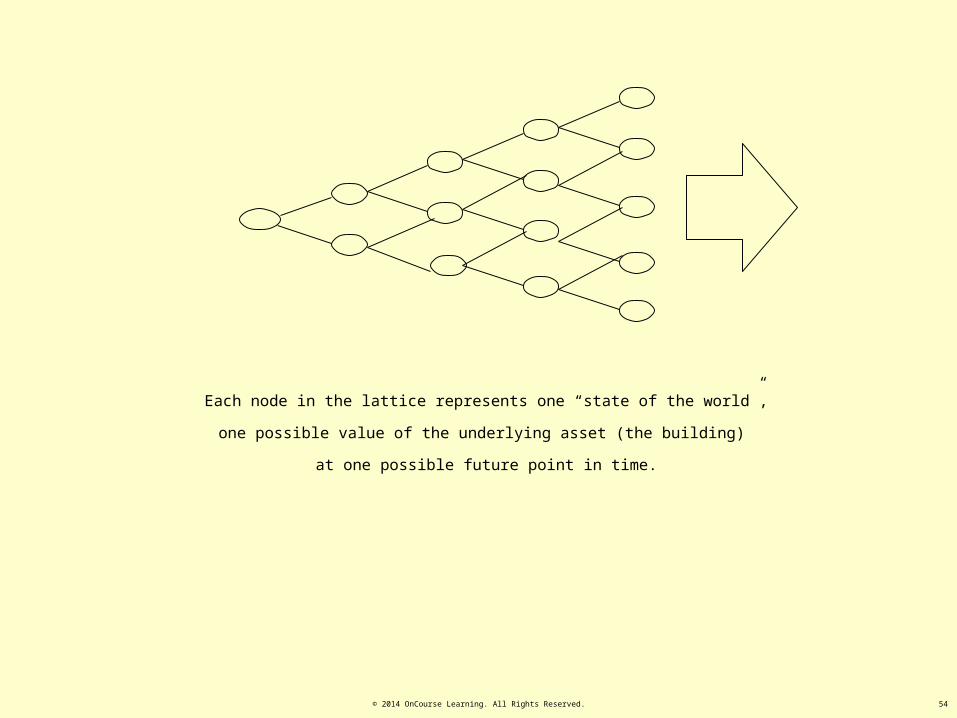
Each node in the lattice represents one “state of the world”,
one possible value of the underlying asset (the building)
at one possible future point in time.

© 2014 OnCourse Learning. All Rights Reserved. 55
t =0 1 2 3 4…
Make three such trees:
“V” value of underlying
asset (bldg)
“K” value of
construction cost
“C” value of option to
get “V” by paying “K”:
(V-K now, or wait…)

© 2014 OnCourse Learning. All Rights Reserved. 56
t =0 1 2 3 4…
Make three such trees:
“V” value of underlying
asset (bldg)
“K” value of
construction cost
“C” value of option to
get “V” by paying “K”:
(V-K now, or wait…)
Base the “C” value on CEQ
method:
MAX[V-K,C]. Compute C lattice
backward from right to left.
“Evolve” (compute) these
lattices forward to reflect
expected growth & volatility,
enumerate future V & K
values…
V-K today, or hold C today based on binomial
possibilities of C next period.
© 2014 OnCourse Learning. All Rights Reserved. 57
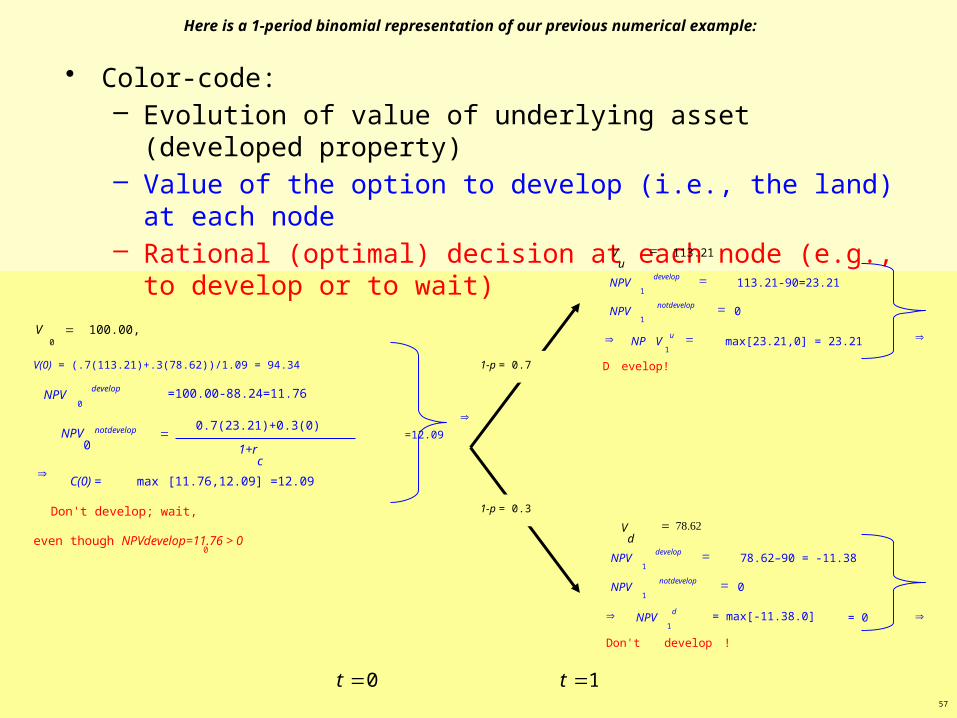
• Color-code:– Evolution of value of underlying asset (developed property)– Value of the option to develop (i.e., the land) at each node– Rational (optimal) decision at each node (e.g., to develop or to wait)
1t 0t
0
0
0
=100.00-88.24=11.76
0.7(23.21)+0.3(0)
max
Don't develop; wait,
even though NPVdevelop=11.76 > 0
[11.76,12.09] =12.09
100.00,
develop
notdevelop
NPV
NPV0
1+r
c
C(0) =
V
=
Þ
=
V(0) = (.7(113.21)+.3(78.62))/1.09 = 94.34
1-p = 0.3
1
1
1
D
113.21-90=23.21
0
max[23.21,0] = 23.21
evelop!
113.21
develop
notdevelop
u
NPV
NPV
NP
Vu
V
=
Þ
=
Þ
=
=
1
1
1
Don't develop
78.62–90 = -11.38
0
= max[-11.38.0]
!
= 0
develop
notdevelop
d
NPV
NPV
NPV
Vd
=
ÞÞ
= 78.62
=
Here is a 1-period binomial representation of our previous numerical example:
=12.09
1-p = 0.7
Þ
© 2014 OnCourse Learning. All Rights Reserved. 58
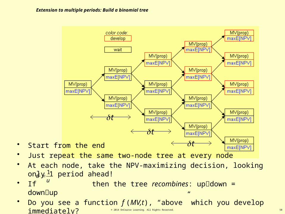
• Start from the end• Just repeat the same two-node tree at every node• At each node, take the NPV-maximizing decision, looking only 1 period ahead!• If then the tree recombines: updown = downup • Do you see a function f (MV,t), “above” which you develop immediately?
1d
u
t
tt
Extension to multiple periods: Build a binomial tree

© 2014 OnCourse Learning. All Rights Reserved. 59
27.4: The Binomial Option Value Model
Think of an individual binomial element (1 period, either “up” or “down”) as like a financial economic “molecule”: the
smallest, simplest representation of the essential characteristics dealt with by financial economics: value over time with risk.
We can have as many periods of time as we want (individual “molecules” stitched together as in a “crystal”: as layers or rows
& columns in a table, or nodes & branches in a “tree).
Each period can represent as short a span of calendar time as we want.
We can have as many periods as we want.
Result:
Binomial “tree” can very realistically model actual evolution of values over time.

© 2014 OnCourse Learning. All Rights Reserved. 60
Appendix 27:
27A.1: The Binomial Option Value Model
Here are the rules for constructing the underlying asset value tree.
Let:
• rV
= Expected total return rate on the underlying asset (built property).
• yV
= Payout rate (dividend yield or net rent yield).
• rf = Riskfree interest rate
• σ = Annual volatility of underlying asset (instantaneous rate)*.
• Vt = Value of the underlying asset at time (end of period) t, ex dividend (i.e., net of current cash payout, i.e., the value of the
asset itself based only on forward-looking cash flows beyond time t). The asset is assumed to pay out cash at a rate of yV
every period: yV
= CFt+1
/ Vt+1
.**
All rates are simple periodic rates:
r = i/m, where r is the simple periodic rate, i is the nominal annual rate, and m is the number of periods per year. The
implied effective annual rate (EAR) is thus given by: 1+EAR = (1+r)m

© 2014 OnCourse Learning. All Rights Reserved. 61
For example, in our previous illustration…
• rV
= 9%
• yV
= 6%
• rf = 3%
• σ = Let’s say this is 20%.
• Vt = $100 at time 0, E[V
t+1] = $102.83 at time 1.
V0
=
$100
V1
up=
$113.21
+ CF1
up = $6.79
= (.06)$113.21
V1
down=
$78.62
+ CF1
down = $4.72
= (.06)$78.62
p = 0.7
1-p = 0.3
E[V1
] = (1.09)$100/(1.06) = $102.83.
E[V1
] = (0.7)$113.62 + (0.3)$78.62 = $102.83.
E[CF1
] = (0.06)$102.83 = $6.17.
E[CF1
] = (0.7)$6.79 + (0.3)$4.72 = $6.17.
“going-in cap rate” = $6.17 / $100 = 6.17%.
E[gV
] = (1+rV
)/(1+yV
) = 1.09/1.06 – 1 = 2.83%
= rV
– (going-in cap rate) = 9% - 6.17%.
$100 =
($102.83 + $6.17) / 1.09
Appendix 27:
27A.1: The Binomial Option Value Model
© 2014 OnCourse Learning. All Rights Reserved. 62
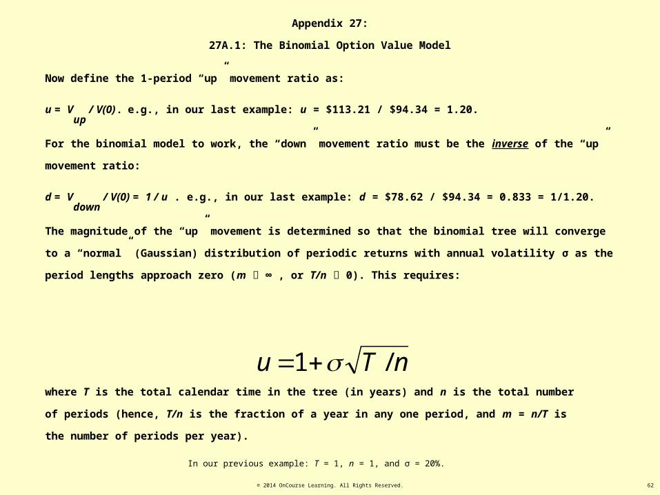
Now define the 1-period “up” movement ratio as:
u = Vup
/ V(0) . e.g., in our last example: u = $113.21 / $94.34 = 1.20.
For the binomial model to work, the “down” movement ratio must be the inverse of the “up” movement ratio:
d = Vdown
/ V(0) = 1 / u . e.g., in our last example: d = $78.62 / $94.34 = 0.833 = 1/1.20.
The magnitude of the “up” movement is determined so that the binomial tree will converge to a “normal” (Gaussian)
distribution of periodic returns with annual volatility σ as the period lengths approach zero (m ∞ , or T/n 0). This requires:
nTu /1 where T is the total calendar time in the tree (in years) and n is the total number of periods (hence, T/n is the fraction of
a year in any one period, and m = n/T is the number of periods per year).
In our previous example: T = 1, n = 1, and σ = 20%.
Appendix 27:
27A.1: The Binomial Option Value Model
© 2014 OnCourse Learning. All Rights Reserved. 63
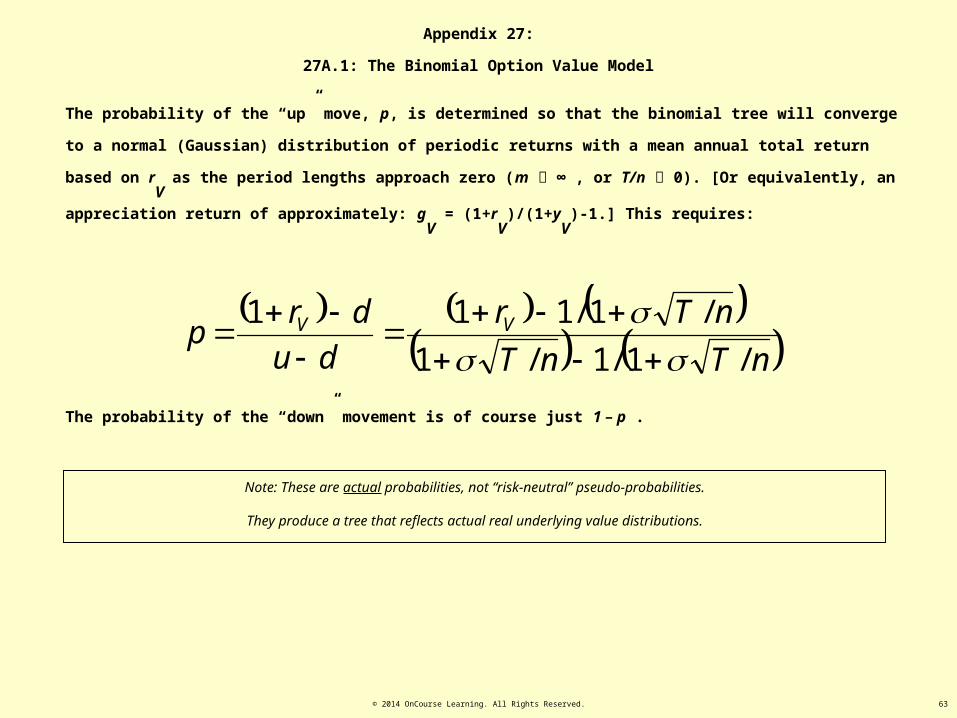
The probability of the “up” move, p, is determined so that the binomial tree will converge to a normal (Gaussian) distribution
of periodic returns with a mean annual total return based on rV
as the period lengths approach zero (m ∞ , or T/n 0). [Or
equivalently, an appreciation return of approximately: gV
= (1+rV
)/(1+yV
)-1.] This requires:
nTnT
nTr
du
drp VV
/1/1/1
/1/111
The probability of the “down” movement is of course just 1 – p .
Note: These are actual probabilities, not “risk-neutral” pseudo-probabilities.
They produce a tree that reflects actual real underlying value distributions.
Appendix 27:
27A.1: The Binomial Option Value Model

© 2014 OnCourse Learning. All Rights Reserved. 64
Example based on our previous illustration
70.0
3667.0
2567.0
833.020.1
833.009.1
20.1120.1
20.1109.1
/1/1/1
/1/111
nTnT
nTr
du
drp VV
The probability of the “down” movement is of course just:
1 – p = 1 – 0.7 = 0.3 .
Appendix 27:
27A.1: The Binomial Option Value Model

© 2014 OnCourse Learning. All Rights Reserved. 65
The binomial tree for the underlying asset ex-dividend values is then constructed as follows.
For any given value node with current (observable) ex-dividend value Vt, the subsequent “up” and “down” values in the
two possible subsequent value nodes are:
VtVtdown
t
VtVtup
t
ynTVydVV
yVnTyuVV
1/11
1/11
1
1
Appendix 27:
27A.1: The Binomial Option Value Model
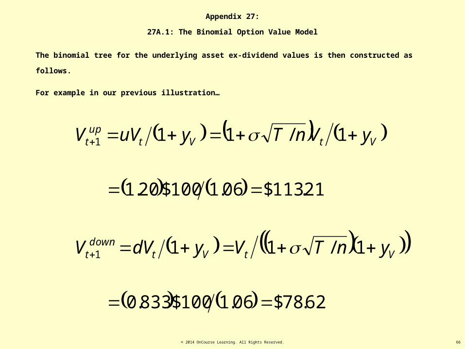
© 2014 OnCourse Learning. All Rights Reserved. 66
The binomial tree for the underlying asset ex-dividend values is then constructed as follows.
For example in our previous illustration…
62.78$06.1100$833.0
1/11
21.113$06.1100$20.1
1/11
1
1
VtVtdown
t
VtVtup
t
ynTVydVV
yVnTyuVV
Appendix 27:
27A.1: The Binomial Option Value Model
© 2014 OnCourse Learning. All Rights Reserved. 67
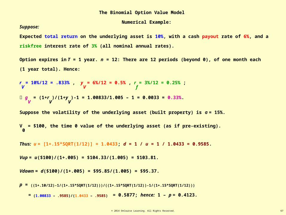
The Binomial Option Value Model
Suppose:
Expected total return on the underlying asset is 10%, with a cash payout rate of 6%, and a riskfree interest rate of 3% (all
nominal annual rates).
Option expires in T = 1 year. n = 12: There are 12 periods (beyond 0), of one month each (1 year total). Hence:
rV
= 10%/12 = .833% , yV
= 6%/12 = 0.5% , rf = 3%/12 = 0.25% ;
gV
= (1+rV
)/(1+yV
)-1 = 1.00833/1.005 – 1 = 0.0033 = 0.33%.
Suppose the volatility of the underlying asset (built property) is σ = 15%.
V0
= $100, the time 0 value of the underlying asset (as if pre-existing).
Thus: u = [1+.15*SQRT(1/12)] = 1.0433; d = 1 / u = 1 / 1.0433 = 0.9585.
Vup = u($100)/(1+.005) = $104.33/(1.005) = $103.81.
Vdown = d($100)/(1+.005) = $95.85/(1.005) = $95.37.
p = ((1+.10/12)-1/(1+.15*SQRT(1/12)))/((1+.15*SQRT(1/12))-1/(1+.15*SQRT(1/12)))
= (1.00833 – .9585)/(1.0433 – .9585) = 0.5877; hence: 1 – p = 0.4123.
Numerical Example:
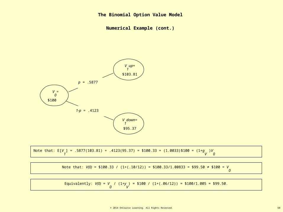
© 2014 OnCourse Learning. All Rights Reserved. 68
The Binomial Option Value Model
Numerical Example (cont.)
V0
=
$100
V1
up=
$103.81
V1
down=
$95.37
p = .5877
1-p = .4123
Note that: V(0) = $100.33 / (1+(.10/12)) = $100.33/1.00833 = $99.50 ≠ $100 = V0
Note that: E[V1
] = .5877(103.81) + .4123(95.37) = $100.33 = (1.0033)$100 = (1+gV
)V0
Equivalently: V(0) = V0
/ (1+yV
) = $100 / (1+(.06/12)) = $100/1.005 = $99.50.

© 2014 OnCourse Learning. All Rights Reserved. 69
V0
=
$100
V1
up=
$103.81
V1
down=
$95.37
p = .5877
1-p = .4123
The Binomial Option Value Model
Now consider the “down” jump from V1
up , and the “up” jump from V1
down (call this value “V1,2
”, because it is in the 1st row down from
the top, 2nd column over from the left in the overall binomial tree).
V1,2
= up from V1
down = u($95.37)/(1+.06/12) = 1.0433(95.37)/1.005 = $99.01.
V1,2
= down from V1
up = d($103.81)/(1+.06/12) = .9585(103.81)/1.005 = $99.01.
This is not a coincidence.
It is a general property of the way we have constructed
the binomial tree. (constant u, d = 1/u.)
It’s the same value!
V1,2
=
$99.01
1-p = .4123
p = .5877

© 2014 OnCourse Learning. All Rights Reserved. 70
V0
=
$100
V1
up=
$103.81
V1
down=
$95.37
p = .5877
1-p = .4123
The Binomial Option Value Model
Here is the tree up through the V0,2
, V1,2
, and V2,2
value nodes . . .
V1,2
=
$99.01
1-p = .4123
p = .5877
We build the underlying asset value tree forward in this manner
V0,2
= up from V1
up = u($ 103.81)/(1+.06/12) = 1.0433(103.81)/1.005 = $107.77.
V2,2
= down from V1
up = d($95.37)/(1+.06/12) = .9585(95.37)/1.005 = $90.96.
V2,2
=
$90.96
V0,2
=
$107.77
1-p = .4123
p = .5877
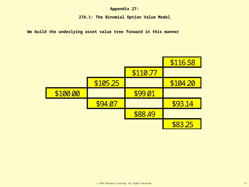
© 2014 OnCourse Learning. All Rights Reserved. 71
We build the underlying asset value tree forward in this manner
$116.58$110.77
$105.25 $104.20$100.00 $99.01
$94.07 $93.14$88.49
$83.25
Appendix 27:
27A.1: The Binomial Option Value Model
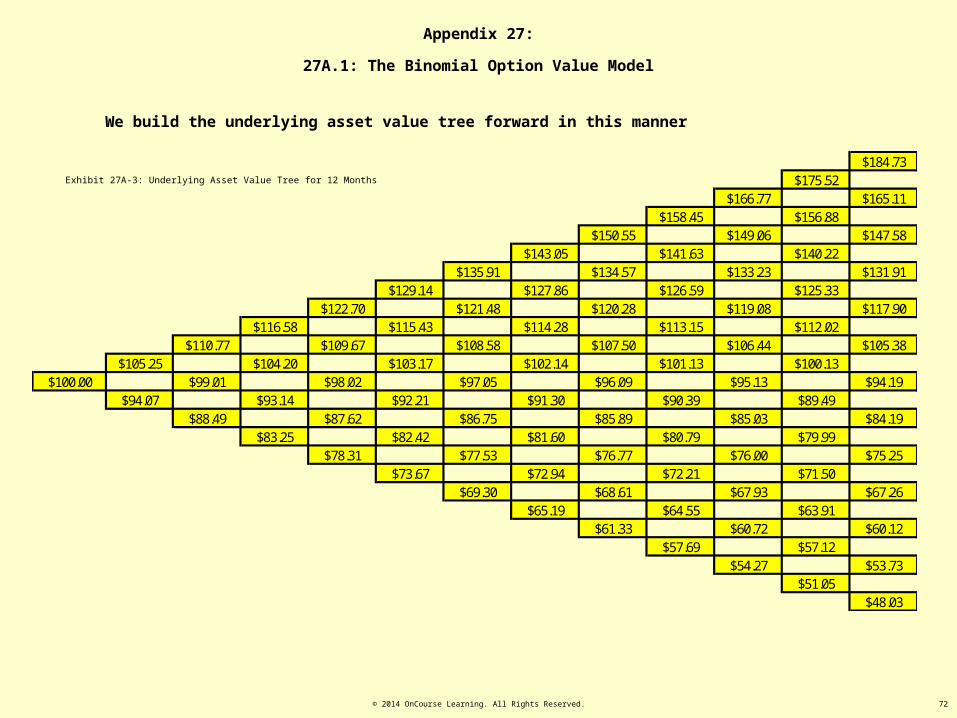
© 2014 OnCourse Learning. All Rights Reserved. 72
We build the underlying asset value tree forward in this manner
$184.73$175.52
$166.77 $165.11$158.45 $156.88
$150.55 $149.06 $147.58$143.05 $141.63 $140.22
$135.91 $134.57 $133.23 $131.91$129.14 $127.86 $126.59 $125.33
$122.70 $121.48 $120.28 $119.08 $117.90$116.58 $115.43 $114.28 $113.15 $112.02
$110.77 $109.67 $108.58 $107.50 $106.44 $105.38$105.25 $104.20 $103.17 $102.14 $101.13 $100.13
$100.00 $99.01 $98.02 $97.05 $96.09 $95.13 $94.19$94.07 $93.14 $92.21 $91.30 $90.39 $89.49
$88.49 $87.62 $86.75 $85.89 $85.03 $84.19$83.25 $82.42 $81.60 $80.79 $79.99
$78.31 $77.53 $76.77 $76.00 $75.25$73.67 $72.94 $72.21 $71.50
$69.30 $68.61 $67.93 $67.26$65.19 $64.55 $63.91
$61.33 $60.72 $60.12$57.69 $57.12
$54.27 $53.73$51.05
$48.03
Appendix 27:
27A.1: The Binomial Option Value Model
Exhibit 27A-3: Underlying Asset Value Tree for 12 Months
© 2014 OnCourse Learning. All Rights Reserved. 73
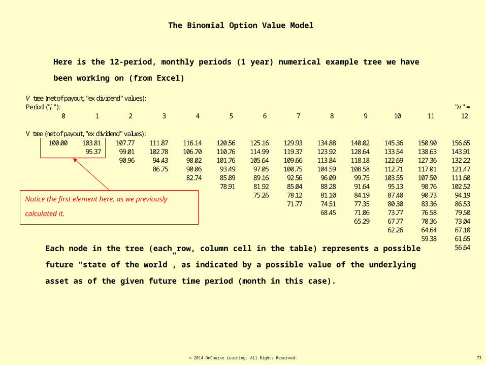
The Binomial Option Value Model
Here is the 12-period, monthly periods (1 year) numerical example tree we have been working on (from Excel)
Notice the first element here, as we previously calculated
it.
Each node in the tree (each row, column cell in the table) represents a possible future “state of the world”, as
indicated by a possible value of the underlying asset as of the given future time period (month in this case).
V tree (net of payout, "ex dividend" values):Period ("j "): "n " =
0 1 2 3 4 5 6 7 8 9 10 11 12
V tree (net of payout, "ex dividend" values):100.00 103.81 107.77 111.87 116.14 120.56 125.16 129.93 134.88 140.02 145.36 150.90 156.65
95.37 99.01 102.78 106.70 110.76 114.99 119.37 123.92 128.64 133.54 138.63 143.9190.96 94.43 98.02 101.76 105.64 109.66 113.84 118.18 122.69 127.36 132.22
86.75 90.06 93.49 97.05 100.75 104.59 108.58 112.71 117.01 121.4782.74 85.89 89.16 92.56 96.09 99.75 103.55 107.50 111.60
78.91 81.92 85.04 88.28 91.64 95.13 98.76 102.5275.26 78.12 81.10 84.19 87.40 90.73 94.19
71.77 74.51 77.35 80.30 83.36 86.5368.45 71.06 73.77 76.58 79.50
65.29 67.77 70.36 73.0462.26 64.64 67.10
59.38 61.6556.64

© 2014 OnCourse Learning. All Rights Reserved. 74
The Binomial Option Value Model
Although the conditional probabilities are p = .5877 and 1-p = .4123 going forward one period (up and down) from any given node, over
multiple periods the unconditional probabilities become bell-shaped over all the possible outcomes
Actually, although the model converges toward continuously-
compounded return probabilities that are normally distributed, the
asset value level probabilities are log-normally distributed (skewed
bell shape).
Tree real probabilities (p based):Period ("j "): "n " =
0 1 2 3 4 5 6 7 8 9 10 11 121.0000 0.5877 0.3454 0.2030 0.1193 0.0701 0.0412 0.0242 0.0142 0.0084 0.0049 0.0029 0.0017
0.4123 0.4846 0.4272 0.3347 0.2459 0.1734 0.1189 0.0798 0.0528 0.0345 0.0223 0.01430.1700 0.2997 0.3523 0.3451 0.3042 0.2503 0.1961 0.1482 0.1088 0.0782 0.0551
0.0701 0.1648 0.2421 0.2846 0.2926 0.2752 0.2426 0.2036 0.1645 0.12890.0289 0.0849 0.1497 0.2053 0.2413 0.2553 0.2500 0.2309 0.2035
0.0119 0.0420 0.0864 0.1355 0.1791 0.2105 0.2268 0.22850.0049 0.0202 0.0475 0.0838 0.1231 0.1591 0.1870
0.0020 0.0095 0.0252 0.0494 0.0798 0.11250.0008 0.0044 0.0130 0.0280 0.0493
0.0003 0.0020 0.0065 0.01540.0001 0.0009 0.0032
0.0001 0.00040.0000
Period 12 Value Probabilities
0%
5%
10%
15%
20%
25%
$57 $62 $67 $73 $80 $87 $94 $103 $112 $121 $132 $144 $157

© 2014 OnCourse Learning. All Rights Reserved. 75
The Binomial Option Value Model
Define the tree as a table of rows and columns. The jth column is the number of periods after the present (time 0), where j = 0, 1, 2, …, n (where n is the
total number of periods). The ith row is the number of “down” moves in the asset price since time 0, where i = 0, 1, 2, … , j . Each row, column cell (i, j)
defines a “state of the world” j periods in the future. Vi,j
is the value of the underlying asset in that state.
The ex ante probability (as of time 0) of any given state of the world i, j is given by:
iij ppiji
jjiprob
1)!(!
!),( )(
where the symbol “!” indicates the “factorial” product operation: x! = 1*2*3* . . . *x.
V tree (net of payout, "ex dividend" values):Period ("j "): "n " =
0 1 2 3 4 5 6 7 8 9 10 11 12
"down" moves ("i"): V tree (net of payout, "ex dividend" values):0 100.00 103.81 107.77 111.87 116.14 120.56 125.16 129.93 134.88 140.02 145.36 150.90 156.651 95.37 99.01 102.78 106.70 110.76 114.99 119.37 123.92 128.64 133.54 138.63 143.912 90.96 94.43 98.02 101.76 105.64 109.66 113.84 118.18 122.69 127.36 132.223 86.75 90.06 93.49 97.05 100.75 104.59 108.58 112.71 117.01 121.474 82.74 85.89 89.16 92.56 96.09 99.75 103.55 107.50 111.605 78.91 81.92 85.04 88.28 91.64 95.13 98.76 102.526 75.26 78.12 81.10 84.19 87.40 90.73 94.197 71.77 74.51 77.35 80.30 83.36 86.538 68.45 71.06 73.77 76.58 79.509 65.29 67.77 70.36 73.04
10 62.26 64.64 67.1011 59.38 61.6512 56.64

© 2014 OnCourse Learning. All Rights Reserved. 76
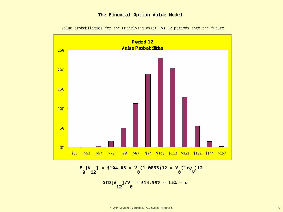
The Binomial Option Value Model
In this numerical example, the Period 12 underlying asset values and probabilities, indicated in the last column on the right
in the previous two slides, give:
E0
[V12
] = E0
[V(1 yr)] = $104.05
which is identical to: V0
((1+rV
)/(1+yV
))12 = V0
(1+gV
)12 = $100(1.0033)12 = $104.05, And:
STD[V12
]/V0
= 1 yr Volatility = ±14.99%
which is very similar to the 15% simple annual volatility assumption.
(If you’re curious, these statistics are found as follows…)
%99.141)!12(!
!12][][
.,5877.0:
05.104$1)!12(!
!12][
0
12
0
)12(212012,012
12,
12
0
)12(12,120
Vppii
VEVVVSTD
tabletheinfoundasareVandpwhere
ppii
VVE
i
iii
i
i
iii
© 2014 OnCourse Learning. All Rights Reserved. 77
The Binomial Option Value Model
E0
[V12
] = $104.05 = V0
(1.0033)12 = V0
(1+gV
)12 .
STD[V12
]/V0
= ±14.99% ≈ 15% = σ
Value probabilities for the underlying asset (V) 12 periods into the future
Period 12 Value Probabilities
0%
5%
10%
15%
20%
25%
$57 $62 $67 $73 $80 $87 $94 $103 $112 $121 $132 $144 $157

© 2014 OnCourse Learning. All Rights Reserved. 78
The Binomial Option Value Model
Period ("j "): "n " =0 1 2 3 4 5 6 7 8 9 10 11 12
"down" moves ("i"): K Value Tree:0 80.00 80.13 80.27 80.40 80.53 80.67 80.80 80.94 81.07 81.21 81.34 81.48 81.611 80.13 80.27 80.40 80.53 80.67 80.80 80.94 81.07 81.21 81.34 81.48 81.612 80.27 80.40 80.53 80.67 80.80 80.94 81.07 81.21 81.34 81.48 81.613 80.40 80.53 80.67 80.80 80.94 81.07 81.21 81.34 81.48 81.614 80.53 80.67 80.80 80.94 81.07 81.21 81.34 81.48 81.615 80.67 80.80 80.94 81.07 81.21 81.34 81.48 81.616 80.80 80.94 81.07 81.21 81.34 81.48 81.617 80.94 81.07 81.21 81.34 81.48 81.618 81.07 81.21 81.34 81.48 81.619 81.21 81.34 81.48 81.61
10 81.34 81.48 81.6111 81.48 81.6112 81.61
For each node (cell) in the underlying asset value tree (the “V Tree” ) described previously, there will also be associated a
projected value of the “exercise price” for the option (the construction cost of the development project).
We label this cost K.
Assuming K grows risklessly at 2%/yr nominal (0.1667%/mo), the table of Ki, j
values giving construction costs
corresponding to the previous Vi, j
values is as follows
© 2014 OnCourse Learning. All Rights Reserved. 79
The Binomial Option Value Model
How to value a call option using the model
While the underlying asset value and exercise price trees are constructed going forward in time as described previously,
An option on the underlying asset is valued by working backward in time, starting at the right-hand edge of the tree
(option expiration) and working back to the left.
The option can be valued one period at a time, at each node of the tree, based on the option values in the two subsequent
possible nodes.
Starting in the last column (expiration period j = n ) one works backwards in time ultimately to the present (time 0 at
period j = 0 ).
Each valuation in each node (i , j cell in the table) is a simple 1-period binomial valuation using the certainty-equivalent
present value model discussed previously.
© 2014 OnCourse Learning. All Rights Reserved. 80
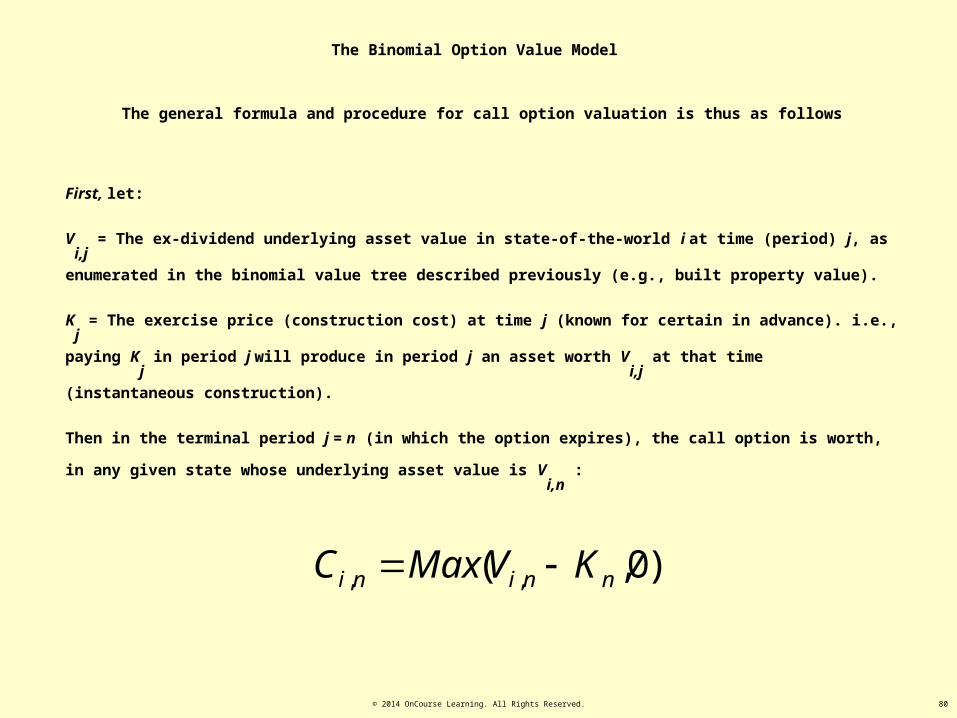
The Binomial Option Value Model
The general formula and procedure for call option valuation is thus as follows
First, let:
Vi,j
= The ex-dividend underlying asset value in state-of-the-world i at time (period) j, as enumerated in the binomial value
tree described previously (e.g., built property value).
Kj = The exercise price (construction cost) at time j (known for certain in advance). i.e., paying K
j in period j will produce in
period j an asset worth Vi,j
at that time (instantaneous construction).
Then in the terminal period j = n (in which the option expires), the call option is worth, in any given state whose underlying
asset value is Vi,n
:
)0,( ,, nnini KVMaxC

© 2014 OnCourse Learning. All Rights Reserved. 81
The Binomial Option Value Model
For example, look at the top two values in the terminal column j = n = 12 of our previous tree, V0,12
= $156.65 and V1,12
=
$143.91 respectively.
Label the value of the call option in each of these nodes: C0,12
and C1,12
.
Given that construction cost in month 12, K12
, is $81.61 (see previous table), we thus have:
C0,12
= Max( $156.65 - $81.61, 0 ) = $75.04
C1,12
= Max( $143.91 - $81.61, 0 ) = $62.30
Now consider the period j = n-1 state from which these two j = n value states are each possible, and suppose (for now) that the
option cannot be exercised prior to its maturity at period n ( “European Option” )…
For example, for the $156.65 and $143.91 values in period 12, this would be the state in period 11 in our previous example
where V0,11
is worth $150.90.
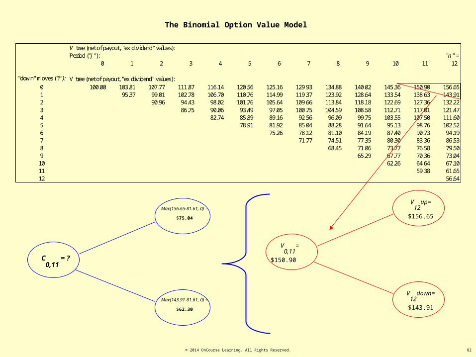
© 2014 OnCourse Learning. All Rights Reserved. 82
The Binomial Option Value Model
V tree (net of payout, "ex dividend" values):Period ("j "): "n " =
0 1 2 3 4 5 6 7 8 9 10 11 12
"down" moves ("i"): V tree (net of payout, "ex dividend" values):0 100.00 103.81 107.77 111.87 116.14 120.56 125.16 129.93 134.88 140.02 145.36 150.90 156.651 95.37 99.01 102.78 106.70 110.76 114.99 119.37 123.92 128.64 133.54 138.63 143.912 90.96 94.43 98.02 101.76 105.64 109.66 113.84 118.18 122.69 127.36 132.223 86.75 90.06 93.49 97.05 100.75 104.59 108.58 112.71 117.01 121.474 82.74 85.89 89.16 92.56 96.09 99.75 103.55 107.50 111.605 78.91 81.92 85.04 88.28 91.64 95.13 98.76 102.526 75.26 78.12 81.10 84.19 87.40 90.73 94.197 71.77 74.51 77.35 80.30 83.36 86.538 68.45 71.06 73.77 76.58 79.509 65.29 67.77 70.36 73.04
10 62.26 64.64 67.1011 59.38 61.6512 56.64
V0,11
=
$150.90
V12
up=
$156.65
V12
down=
$143.91
C0,11
= ?
Max(156.65-81.61, 0) =
$75.04
Max(143.91-81.61, 0) =
$62.30
© 2014 OnCourse Learning. All Rights Reserved. 83
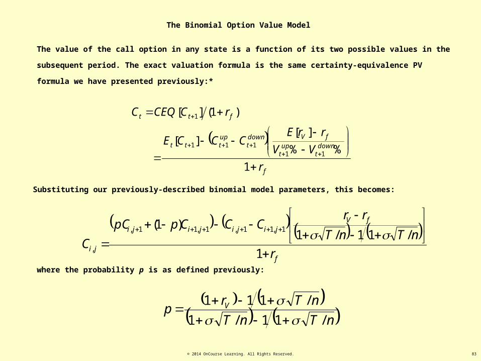
The Binomial Option Value Model
The value of the call option in any state is a function of its two possible values in the subsequent period. The exact valuation
formula is the same certainty-equivalence PV formula we have presented previously:*
f
downt
upt
fVdownt
upttt
ftt
r
VV
rrECCCE
rCCEQC
1
%%
][][
)1(][
11111
1
Substituting our previously-described binomial model parameters, this becomes:
nTnT
nTrp V
/11/1
/111
where the probability p is as defined previously:
f
fVjijijiji
ji r
nTnT
rrCCCppC
C
1
/11/1)1( 1,11,1,11,
,

© 2014 OnCourse Learning. All Rights Reserved. 84
The Binomial Option Value Model
In particular, for C0,11
, recalling our previous 1-year monthly numerical example input parameters of: rV
= 10%/12
= .833% , yV
= 6%/12 = 0.5% , rf
= 3%/12 = 0.25%, and σ = 15%, we obtain:
73.68$
0025.191.68$
0025.10688.073.12$78.69$
0025.1%48.8%583.0
30.6204.75)30.62(4123.)04.75(5877.
0025.1%85.95%33.104
%25.0%833.0412.5877.
)1(12/11112/11
4123.5877.
12,212,112,112,0
12,112,012,112,011,0
CCCC
rrr
CCCCC ffV

© 2014 OnCourse Learning. All Rights Reserved. 85
The Binomial Option Value Model
V0,11
=
$150.90
V12
up=
$156.65
V12
down=
$143.91
C0,11
= $68.73
C0,12
=
$75.03
C1,12
=
$62.30
73.68$
0025.191.68$
)12/%31(12/1%151112/1%151
12/%312/%1030.6203.75)30.62(4123.)03.75(5877.
)1(12/1112/11
)1( 12,112,012,112,011,0
f
fV rrr
CCCppCC
K12
= $81.61
K11
= $81.48

© 2014 OnCourse Learning. All Rights Reserved. 86
The Binomial Option Value Model
Repeating this process within each column for i = 0, 1, 2, …, j , and then across columns from right to left for j = 11, 10, 9, …,
0 , we eventually obtain the value of the option as of the present time 0:
Period ("j "): "n " =0 1 2 3 4 5 6 7 8 9 10 11 12
"down" moves ("i"): Eurpoean Call Option Value Tree:0 15.76 19.23 23.06 27.20 31.60 36.23 41.07 46.13 51.41 56.94 62.71 68.73 75.031 12.09 15.20 18.72 22.60 26.78 31.19 35.83 40.67 45.72 51.01 56.53 62.302 8.81 11.48 14.63 18.21 22.15 26.36 30.79 35.42 40.26 45.32 50.603 5.97 8.15 10.85 14.06 17.72 21.72 25.96 30.39 35.02 39.854 3.64 5.27 7.44 10.19 13.50 17.26 21.32 25.55 29.985 1.90 2.97 4.51 6.67 9.51 12.98 16.86 20.916 0.77 1.31 2.21 3.64 5.81 8.87 12.587 0.18 0.35 0.68 1.32 2.55 4.928 0.00 0.00 0.00 0.00 0.009 0.00 0.00 0.00 0.00
10 0.00 0.00 0.0011 0.00 0.0012 0.00
The European option is worth $15.76 in the present time 0.
Note here the values we calculated in the previous slides.*
© 2014 OnCourse Learning. All Rights Reserved. 87
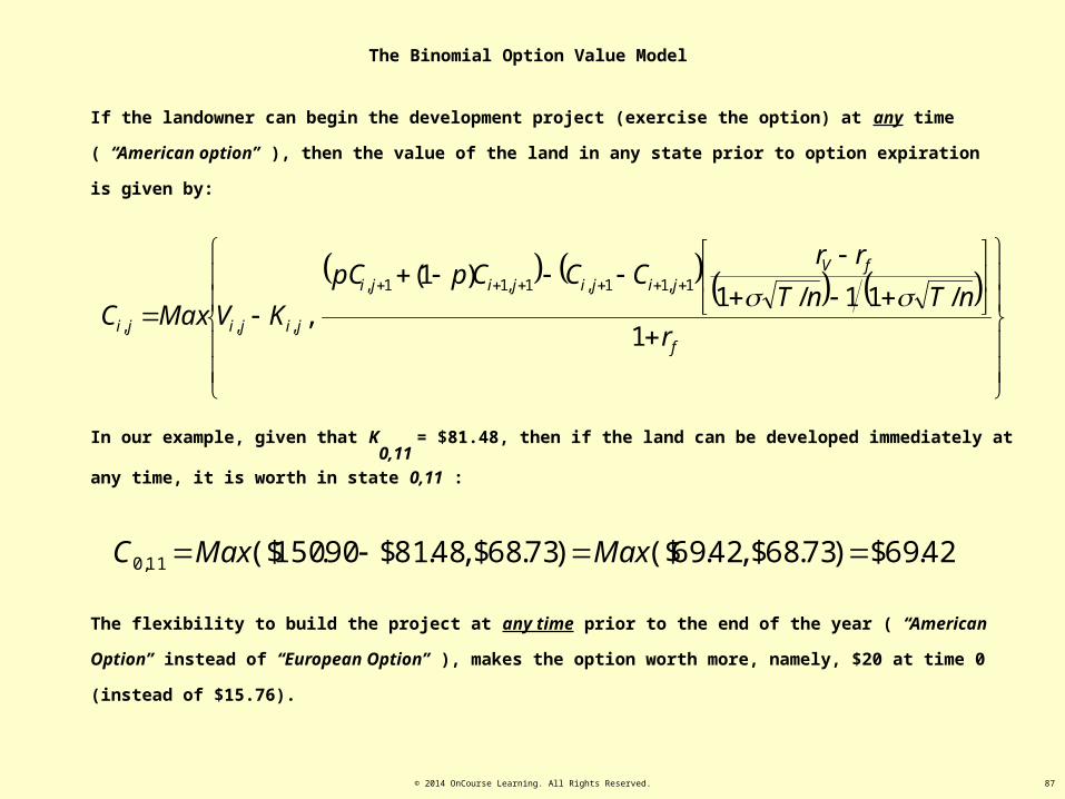
The Binomial Option Value Model
In our example, given that K0,11
= $81.48, then if the land can be developed immediately at any time, it is worth in state 0,11 :
42.69$)73.68$,42.69($)73.68$,48.81$90.150($11,0 MaxMaxC
If the landowner can begin the development project (exercise the option) at any time ( “American option” ), then the value of
the land in any state prior to option expiration is given by:
f
fVjijijiji
jijiji r
nTnT
rrCCCppC
KVMaxC1
/11/1)1(
,1,11,1,11,
,,,
The flexibility to build the project at any time prior to the end of the year ( “American Option” instead of “European Option” ),
makes the option worth more, namely, $20 at time 0 (instead of $15.76).
© 2014 OnCourse Learning. All Rights Reserved. 88
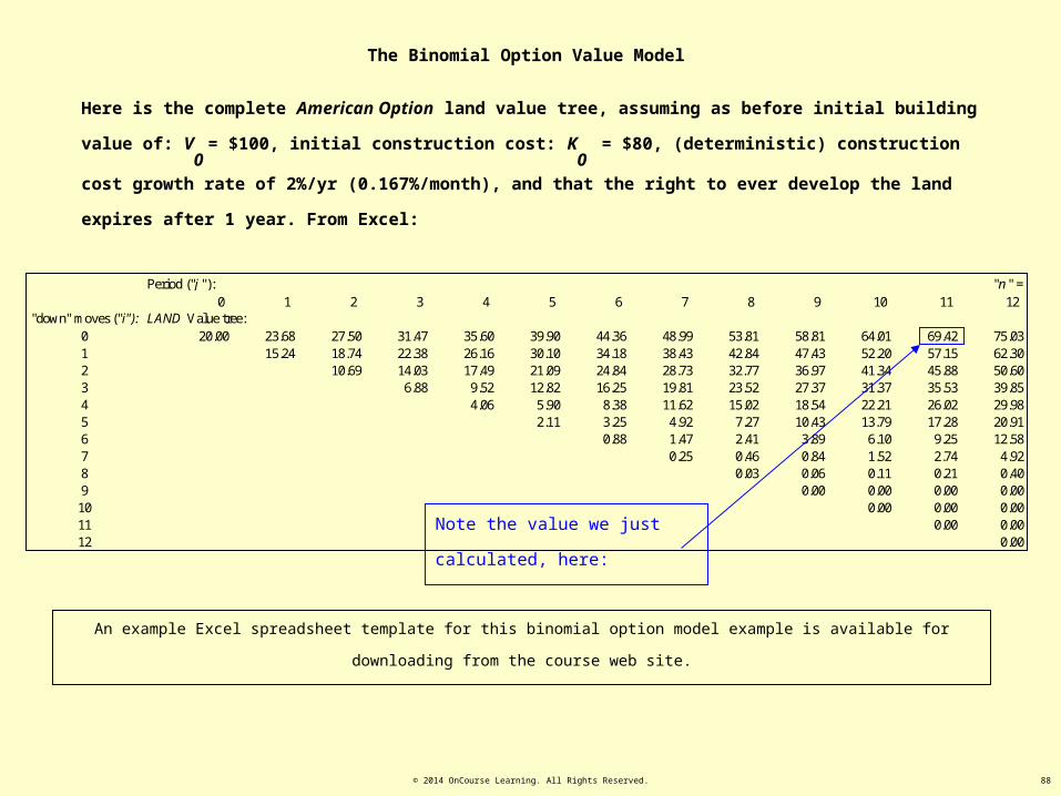
The Binomial Option Value Model
Here is the complete American Option land value tree, assuming as before initial building value of: V0
= $100, initial
construction cost: K0
= $80, (deterministic) construction cost growth rate of 2%/yr (0.167%/month), and that the right to
ever develop the land expires after 1 year. From Excel:
An example Excel spreadsheet template for this binomial option model example is available for downloading from the course web site.
Period ("j "): "n " =0 1 2 3 4 5 6 7 8 9 10 11 12
"down" moves ("i"): LAND Value tree:0 20.00 23.68 27.50 31.47 35.60 39.90 44.36 48.99 53.81 58.81 64.01 69.42 75.031 15.24 18.74 22.38 26.16 30.10 34.18 38.43 42.84 47.43 52.20 57.15 62.302 10.69 14.03 17.49 21.09 24.84 28.73 32.77 36.97 41.34 45.88 50.603 6.88 9.52 12.82 16.25 19.81 23.52 27.37 31.37 35.53 39.854 4.06 5.90 8.38 11.62 15.02 18.54 22.21 26.02 29.985 2.11 3.25 4.92 7.27 10.43 13.79 17.28 20.916 0.88 1.47 2.41 3.89 6.10 9.25 12.587 0.25 0.46 0.84 1.52 2.74 4.928 0.03 0.06 0.11 0.21 0.409 0.00 0.00 0.00 0.00
10 0.00 0.00 0.0011 0.00 0.0012 0.00
Note the value we just calculated,
here:
© 2014 OnCourse Learning. All Rights Reserved. 89
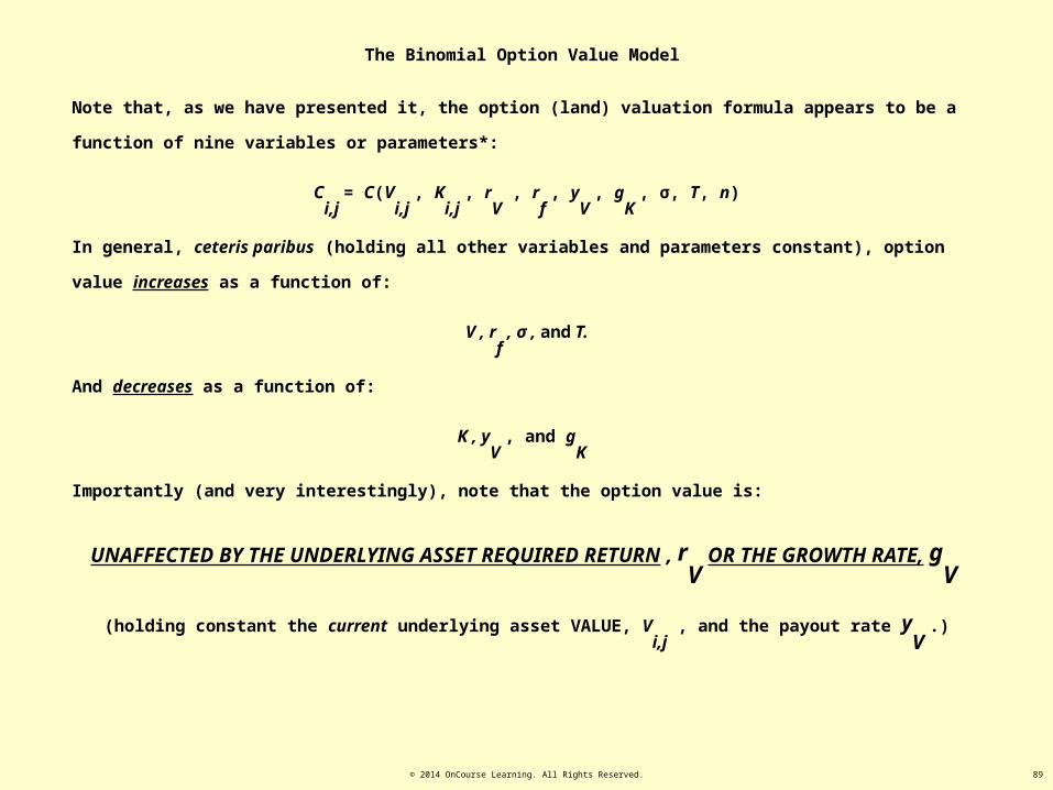
The Binomial Option Value Model
Note that, as we have presented it, the option (land) valuation formula appears to be a function of nine variables or
parameters*:
Ci,j
= C(Vi,j
, Ki,j
, rV
, rf , y
V , g
K , σ, T, n)
In general, ceteris paribus (holding all other variables and parameters constant), option value increases as a function of:
V , rf , σ , and T.
And decreases as a function of:
K , yV
, and gK
Importantly (and very interestingly), note that the option value is:
UNAFFECTED BY THE UNDERLYING ASSET REQUIRED RETURN , rV
OR THE GROWTH RATE,
gV
(holding constant the current underlying asset VALUE, Vi,j
, and the payout rate yV
.)
Also, recall accounting relationship that must hold:
(1+rV
) =(1+yV
) (1+gV
), rV
≈ yV
+ gV 90
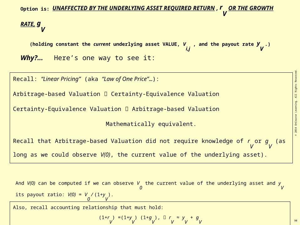
Option is: UNAFFECTED BY THE UNDERLYING ASSET REQUIRED RETURN , rV
OR THE
GROWTH RATE, gV
(holding constant the current underlying asset VALUE, Vi,j
, and the payout rate yV
.)
Why?... Here’s one way to see it:
Recall: “Linear Pricing” (aka “Law of One Price”…):
Arbitrage-based Valuation Certainty-Equivalence Valuation
Certainty-Equivalence Valuation Arbitrage-based Valuation
Mathematically equivalent.
Recall that Arbitrage-based Valuation did not require knowledge of rV
or gV
(as long as we could observe
V(0), the current value of the underlying asset).
And V(0) can be computed if we can observe V0
the current value of the underlying asset and yV
its payout ratio: V(0) = V0
/
(1+yV
).
© 2
014
OnC
ours
e Le
arni
ng. A
ll Ri
ghts
Res
erve
d.

© 2014 OnCourse Learning. All Rights Reserved. 91
The Binomial Option Value Model
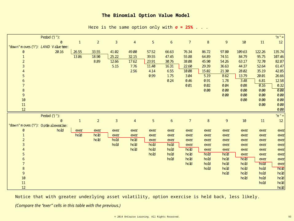
Effect of Underlying Asset Volatility
This is the same option as before only we’ve increased the underlying asset volatility (σ) from 15% to 25%.
Period ("j "): "n " =0 1 2 3 4 5 6 7 8 9 10 11 12
"down" moves ("i"): LAND Value tree:0 20.16 26.55 33.55 41.02 49.00 57.52 66.63 76.34 86.72 97.80 109.63 122.26 135.741 13.86 18.90 25.22 32.15 39.55 47.45 55.88 64.89 74.51 84.79 95.75 107.462 8.89 12.66 17.62 23.91 30.76 38.08 45.90 54.26 63.17 72.70 82.873 5.15 7.76 11.40 16.31 22.60 29.39 36.63 44.37 52.64 61.474 2.56 4.14 6.55 10.08 15.02 21.30 28.02 35.19 42.855 0.99 1.75 3.04 5.19 8.62 13.79 20.01 26.666 0.24 0.46 0.91 1.78 3.48 6.81 12.587 0.01 0.02 0.04 0.08 0.16 0.328 0.00 0.00 0.00 0.00 0.009 0.00 0.00 0.00 0.00
10 0.00 0.00 0.0011 0.00 0.0012 0.00
Note the increase in value from
$20.00 to $20.16
With 15% volatility, the option model called for optimal immediate exercise at time 0.
With 25% volatility, the model indicates that the option is more valuable held for speculation at time 0 instead of immediate
exercise at that time.

© 2014 OnCourse Learning. All Rights Reserved. 92
Period ("j "): "n " =0 1 2 3 4 5 6 7 8 9 10 11 12
"down" moves ("i"): Optimal exercise:0 exer exer exer exer exer exer exer exer exer exer exer exer exer1 exer exer exer exer exer exer exer exer exer exer exer exer2 exer exer exer exer exer exer exer exer exer exer exer3 hold exer exer exer exer exer exer exer exer exer4 hold hold hold exer exer exer exer exer exer5 hold hold hold hold exer exer exer exer6 hold hold hold hold hold exer exer7 hold hold hold hold hold exer8 hold hold hold hold hold9 hold hold hold hold
10 hold hold hold11 hold hold12 hold
The Binomial Option Value Model
Notice that the option value model not only values the option, but also indicates in which states of the world it is optimal to exercise the option (build
the development project). Here are the valuation and optimal exercise trees for the option with σ back at the original 15%
Period ("j "): "n " =0 1 2 3 4 5 6 7 8 9 10 11 12
"down" moves ("i"): LAND Value tree:0 20.00 23.68 27.50 31.47 35.60 39.90 44.36 48.99 53.81 58.81 64.01 69.42 75.031 15.24 18.74 22.38 26.16 30.10 34.18 38.43 42.84 47.43 52.20 57.15 62.302 10.69 14.03 17.49 21.09 24.84 28.73 32.77 36.97 41.34 45.88 50.603 6.88 9.52 12.82 16.25 19.81 23.52 27.37 31.37 35.53 39.854 4.06 5.90 8.38 11.62 15.02 18.54 22.21 26.02 29.985 2.11 3.25 4.92 7.27 10.43 13.79 17.28 20.916 0.88 1.47 2.41 3.89 6.10 9.25 12.587 0.25 0.46 0.84 1.52 2.74 4.928 0.03 0.06 0.11 0.21 0.409 0.00 0.00 0.00 0.00
10 0.00 0.00 0.0011 0.00 0.0012 0.00
© 2014 OnCourse Learning. All Rights Reserved. 93
The Binomial Option Value Model
Here is the same option only with σ = 25% . . .
Period ("j "): "n " =0 1 2 3 4 5 6 7 8 9 10 11 12
"down" moves ("i"): LAND Value tree:0 20.16 26.55 33.55 41.02 49.00 57.52 66.63 76.34 86.72 97.80 109.63 122.26 135.741 13.86 18.90 25.22 32.15 39.55 47.45 55.88 64.89 74.51 84.79 95.75 107.462 8.89 12.66 17.62 23.91 30.76 38.08 45.90 54.26 63.17 72.70 82.873 5.15 7.76 11.40 16.31 22.60 29.39 36.63 44.37 52.64 61.474 2.56 4.14 6.55 10.08 15.02 21.30 28.02 35.19 42.855 0.99 1.75 3.04 5.19 8.62 13.79 20.01 26.666 0.24 0.46 0.91 1.78 3.48 6.81 12.587 0.01 0.02 0.04 0.08 0.16 0.328 0.00 0.00 0.00 0.00 0.009 0.00 0.00 0.00 0.00
10 0.00 0.00 0.0011 0.00 0.0012 0.00
Notice that with greater underlying asset volatility, option exercise is held back, less likely. (Compare the “exer” cells in this table with the previous.)
Period ("j "): "n " =0 1 2 3 4 5 6 7 8 9 10 11 12
"down" moves ("i"): Optimal exercise:0 hold exer exer exer exer exer exer exer exer exer exer exer exer1 hold hold exer exer exer exer exer exer exer exer exer exer2 hold hold hold exer exer exer exer exer exer exer exer3 hold hold hold hold exer exer exer exer exer exer4 hold hold hold hold exer exer exer exer exer5 hold hold hold hold hold exer exer exer6 hold hold hold hold hold exer exer7 hold hold hold hold hold exer8 hold hold hold hold hold9 hold hold hold hold
10 hold hold hold11 hold hold12 hold

© 2014 OnCourse Learning. All Rights Reserved. 94
Period ("j "): "n " =0 1 2 3 4 5 6 7 8 9 10 11 12
"down" moves ("i"): Optimal exercise:0 exer exer exer exer exer exer exer exer exer exer exer exer exer1 exer exer exer exer exer exer exer exer exer exer exer exer2 exer exer exer exer exer exer exer exer exer exer exer3 hold exer exer exer exer exer exer exer exer exer4 hold hold hold exer exer exer exer exer exer5 hold hold hold hold exer exer exer exer6 hold hold hold hold hold exer exer7 hold hold hold hold hold exer8 hold hold hold hold hold9 hold hold hold hold
10 hold hold hold11 hold hold12 hold
The Binomial Option Value Model
With 15% volatility, immediate exercise.
Period ("j "): "n " =0 1 2 3 4 5 6 7 8 9 10 11 12
"down" moves ("i"): Optimal exercise:0 hold exer exer exer exer exer exer exer exer exer exer exer exer1 hold hold exer exer exer exer exer exer exer exer exer exer2 hold hold hold exer exer exer exer exer exer exer exer3 hold hold hold hold exer exer exer exer exer exer4 hold hold hold hold exer exer exer exer exer5 hold hold hold hold hold exer exer exer6 hold hold hold hold hold exer exer7 hold hold hold hold hold exer8 hold hold hold hold hold9 hold hold hold hold
10 hold hold hold11 hold hold12 hold
With 25% volatility, delay construction.

© 2014 OnCourse Learning. All Rights Reserved. 95
The Binomial Option Value Model
Risk & the OCC
What are the implications of the option model for the amount of investment risk, and the corresponding risk-adjusted discount
rate (OCC ) applicable to the land?
For a finite-lived option, the risk and OCC will differ according to the “state-of-the-world” (the V, and K values, and the time
until option expiration).
But recall that the certainty-equivalence valuation we are employing here allows us to “back out” what is the OCC once we have
computed the option value. The formula to do this is obtained as follows:
][
][11
,1
][
][1
][
1
][
1
1,
,
111,
,
j
jjfji
ji
jj
Cf
jj
f
jji
CCEQ
CErOCC
OCC
CE
RPEr
CE
r
CCEQC
ji
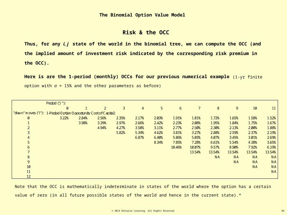
© 2014 OnCourse Learning. All Rights Reserved. 96
Risk & the OCC
Thus, for any i, j state of the world in the binomial tree, we can compute the OCC (and the implied amount of investment
risk indicated by the corresponding risk premium in the OCC).
Here is are the 1-period (monthly) OCCs for our previous numerical example (1-yr finite option with σ = 15% and the other
parameters as before)
The Binomial Option Value Model
Period ("j "):0 1 2 3 4 5 6 7 8 9 10 11
"down" moves ("i"): 1-Period Option Opportunity Cost of Capital:0 3.22% 2.84% 2.56% 2.35% 2.17% 2.03% 1.91% 1.81% 1.72% 1.65% 1.58% 1.52%1 3.98% 3.39% 2.97% 2.66% 2.42% 2.23% 2.08% 1.95% 1.84% 1.75% 1.67%2 4.94% 4.27% 3.58% 3.11% 2.77% 2.50% 2.30% 2.13% 2.00% 1.88%3 5.82% 5.34% 4.62% 3.81% 3.27% 2.88% 2.59% 2.37% 2.19%4 6.87% 6.40% 5.86% 5.03% 4.07% 3.45% 3.01% 2.69%5 8.34% 7.85% 7.28% 6.61% 5.54% 4.38% 3.65%6 10.46% 10.07% 9.57% 8.90% 7.92% 6.19%7 13.54% 13.54% 13.54% 13.54% 13.54%8 NA NA NA NA9 NA NA NA
10 NA NA11 NA12
Note that the OCC is mathematically indeterminate in states of the world where the option has a certain value of zero (in all future possible states of the
world and hence in the current state).*

© 2014 OnCourse Learning. All Rights Reserved. 97
Period ("j "):0 1 2 3 4 5 6 7 8 9 10 11
"down" moves ("i"): Option Opportunity Cost of Capital per Annum (EAR):0 46.2% 40.0% 35.5% 32.1% 29.4% 27.2% 25.5% 24.0% 22.7% 21.7% 20.7% 19.9%1 59.8% 49.2% 42.1% 37.0% 33.3% 30.3% 28.0% 26.1% 24.5% 23.2% 22.0%2 78.3% 65.2% 52.6% 44.4% 38.7% 34.5% 31.3% 28.8% 26.8% 25.1%3 97.2% 86.7% 71.9% 56.6% 47.1% 40.6% 36.0% 32.4% 29.7%4 121.9% 110.5% 98.1% 80.2% 61.4% 50.2% 42.8% 37.5%5 161.6% 147.8% 132.4% 115.6% 91.1% 67.2% 53.8%6 229.8% 216.2% 199.4% 178.3% 149.7% 105.5%7 358.9% 358.9% 358.9% 358.9% 358.9%8 NA NA NA NA9 NA NA NA
10 NA NA11 NA
Risk & the OCC
Here are the per annum (effective annual rates) expected returns implied by the preceding periodic OCCs
The Binomial Option Value Model
Note: These OCCs are probably not very realistic (too high) for actual land investment, because of our assumption here of a 1-year finite life of
the development option. In reality, land development rights typically do not expire at the end of a year. (More on this shortly.)

© 2014 OnCourse Learning. All Rights Reserved. 98
Risk & the OCC
How do these option OCCs compare to the “Method 1” (“canonical”) Formula for the OCC of a development project,
introduced in the Chapter 29 lecture notes?
The Binomial Option Value Model
Recall that the Method 1 Formula is as follows (where TC
is the time required for construction):
Recasting this in our current nomenclature with TC
= 1 yr , this formula is:
1
1][1
1][][
1
11
,
KrVEr
rKVErE
Vjjf
fjjjC ji
This formula will in fact be equivalent to the option OCC previously computed in any state of the world where the option
will definitely be exercised in the next period. (Recall that the canonical formula assumes a definite commitment to go forward with the
development project.)
1][1][1
][1][1][
1
C
CC
CCT
TT
VTT
D
TD
TVTT
CLrEVrE
rErELVrE
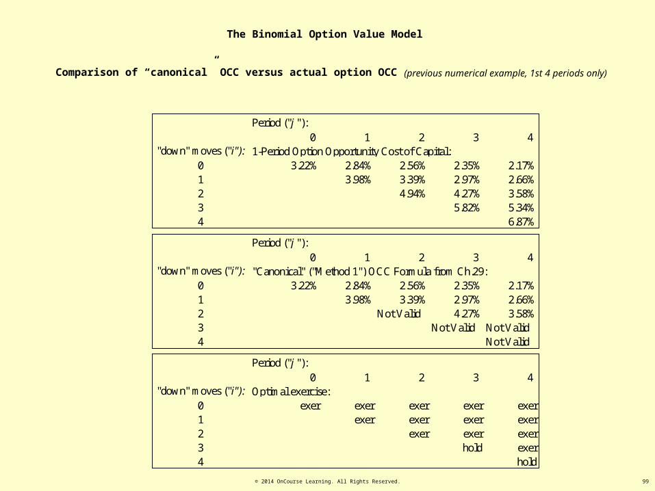
© 2014 OnCourse Learning. All Rights Reserved. 99
Comparison of “canonical” OCC versus actual option OCC (previous numerical example, 1st 4 periods only)
The Binomial Option Value Model
Period ("j "):0 1 2 3 4
"down" moves ("i"): "Canonical" ("Method 1") OCC Formula from Ch.29:0 3.22% 2.84% 2.56% 2.35% 2.17%1 3.98% 3.39% 2.97% 2.66%2 Not Valid 4.27% 3.58%3 Not Valid Not Valid4 Not Valid
Period ("j "):0 1 2 3 4
"down" moves ("i"): 1-Period Option Opportunity Cost of Capital:0 3.22% 2.84% 2.56% 2.35% 2.17%1 3.98% 3.39% 2.97% 2.66%2 4.94% 4.27% 3.58%3 5.82% 5.34%4 6.87%
Period ("j "):0 1 2 3 4
"down" moves ("i"): Optimal exercise:0 exer exer exer exer exer1 exer exer exer exer2 exer exer exer3 hold exer4 hold

© 2014 OnCourse Learning. All Rights Reserved. 100
Problems with the Binomial Model
There are two major technical problems with the Binomial Model:
1. Discrete time & values (the real world is continuous).
2. Finite expiration of the option (land is perpetual).
Both of these can have significant effects on the option value and optimal exercise decision characteristics.
The first problem (discreteness) can be addressed by making the periods of time very short (m ∞, T/n 0).
Perpetual expiration can be approximated by a long time horizon, but more accurate solution requires an entirely different
type of model.
For modeling a simple option, sufficient for dealing with the Wait Option, there is a simple solution to this problem:
A model of perpetual option value in continuous time that includes the value of the option to delay construction as well as a
solution to the decision problem of optimal development timing . . .
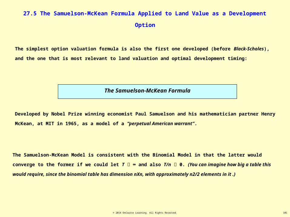
© 2014 OnCourse Learning. All Rights Reserved. 101
27.5 The Samuelson-McKean Formula Applied to Land Value as a Development Option
The simplest option valuation formula is also the first one developed (before Black-Scholes), and the one that is most relevant to
land valuation and optimal development timing:
The Samuelson-McKean Formula
Developed by Nobel Prize winning economist Paul Samuelson and his mathematician partner Henry McKean, at MIT in 1965, as a
model of a “perpetual American warrant”.
The Samuelson-McKean Model is consistent with the Binomial Model in that the latter would converge to the former if we could let
T ∞ and also T/n 0. (You can imagine how big a table this would require, since the binomial table has dimension nXn, with
approximately n2/2 elements in it .)

© 2014 OnCourse Learning. All Rights Reserved. 102
To see how this works, recall our replicating portfolio model of option value
Today Next Year
Development Option Value C(0)=x“x” = unknown val.
C(t)UP=113.21-90
= $23.21
C(t)DOWN = 0
(Don’t build)
Built Property Value V(0) = V0 / (1+yV) = $102.83/(1.09)
=$94.34
V(t)UP= $113.21 V(t)DOWN= $78.62
Bond Value B = $51.21 B(t) = (1+rf )B = $52.74
B(t) = (1+rf )B = $52.74
Replicating Portfolio:C(0) = (N)V(0) – B
C(0) = (N)V(0) – B = (0.7)$94.34 -
$51.21 = $12.09
C(t)UP =
(0.7)113.21 - $52.74 = $23.21
C(t)DOWN =
(0.7)78.62 - $52.74 = 0
The Replicating Portfolio = NV-B, where: N=(Cu-Cd)/(Vu-Vd); B=(NVd-Cd)/(1+rf); and V = V(0) (not V
0 )
BVV
C
r
CVVV
CC
VVV
CCC
f
DOWNt
DOWNtDOWN
tUP
t
DOWNt
UPt
DOWNt
UPt
DOWNt
UPt
)0(1
)0(0
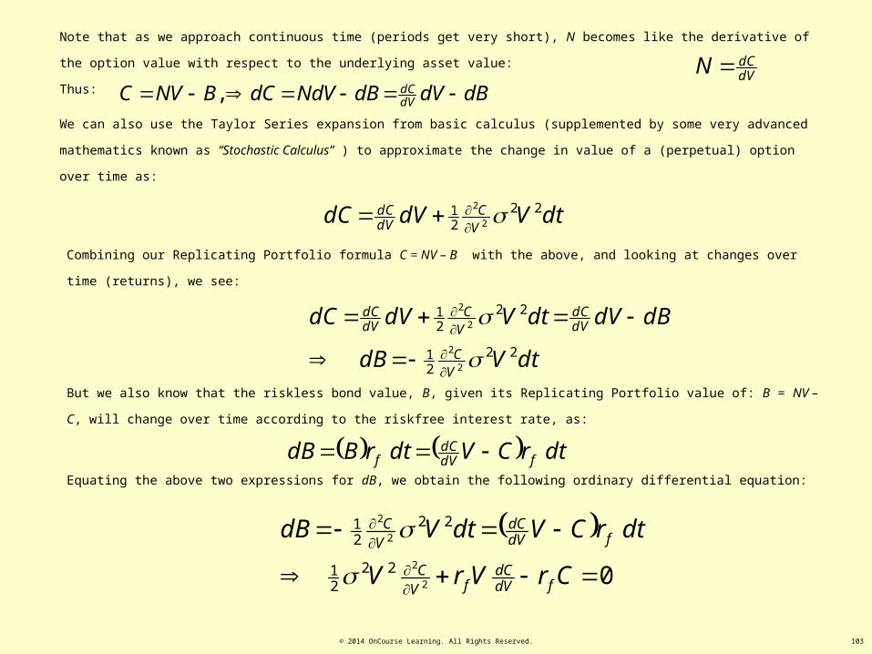
© 2014 OnCourse Learning. All Rights Reserved. 103
Note that as we approach continuous time (periods get very short), N becomes like the derivative of the option value with respect to the underlying
asset value:
Thus:
dtVdVdCV
CdVdC 22
21
2
2
Combining our Replicating Portfolio formula C = NV – B with the above, and looking at changes over time (returns), we see:
dtVdB
dBdVdtVdVdC
VC
dVdC
VC
dVdC
2221
2221
2
2
2
2
But we also know that the riskless bond value, B, given its Replicating Portfolio value of: B = NV – C, will change over time according to the riskfree
interest rate, as:
dtrCVdtrBdB fdVdC
f
We can also use the Taylor Series expansion from basic calculus (supplemented by some very advanced mathematics known as “Stochastic Calculus”
) to approximate the change in value of a (perpetual) option over time as:
dVdCN
dBdVdBNdVdCBNVC dVdC ,
Equating the above two expressions for dB, we obtain the following ordinary differential equation:
02
2
2
2
2221
2221
CrVrV
dtrCVdtVdB
fdVdC
fVC
fdVdC
VC
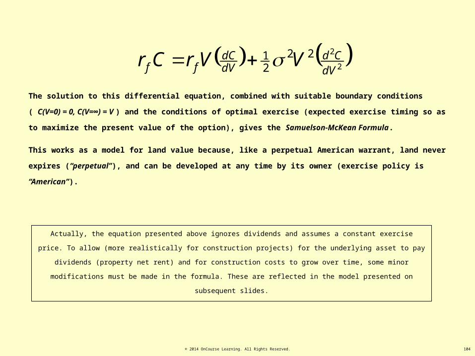
© 2014 OnCourse Learning. All Rights Reserved. 104
2
22221
dVCd
dVdC
ff VVrCr
The solution to this differential equation, combined with suitable boundary conditions ( C(V=0) = 0, C(V=∞) = V ) and the
conditions of optimal exercise (expected exercise timing so as to maximize the present value of the option), gives the Samuelson-
McKean Formula.
This works as a model for land value because, like a perpetual American warrant, land never expires (“perpetual”), and can be
developed at any time by its owner (exercise policy is “American”).
Actually, the equation presented above ignores dividends and assumes a constant exercise price. To allow (more realistically for
construction projects) for the underlying asset to pay dividends (property net rent) and for construction costs to grow over time, some minor
modifications must be made in the formula. These are reflected in the model presented on subsequent slides.
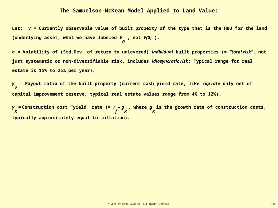
© 2014 OnCourse Learning. All Rights Reserved. 105
The Samuelson-McKean Model Applied to Land Value:
Let: V = Currently observable value of built property of the type that is the HBU for the land (underlying asset, what we have labeled
V0
, not V(0) ).
σ = Volatility of (Std.Dev. of return to unlevered) individual built properties (= “total risk”, not just systematic or non-diversifiable
risk, includes idiosyncratic risk: Typical range for real estate is 15% to 25% per year).
yV
= Payout ratio of the built property (current cash yield rate, like cap rate only net of capital improvement reserve, typical real
estate values range from 4% to 12%).
yK
= Construction cost “yield” rate (= rf – g
K , where g
K is the growth rate of construction costs, typically approximately equal to
inflation).
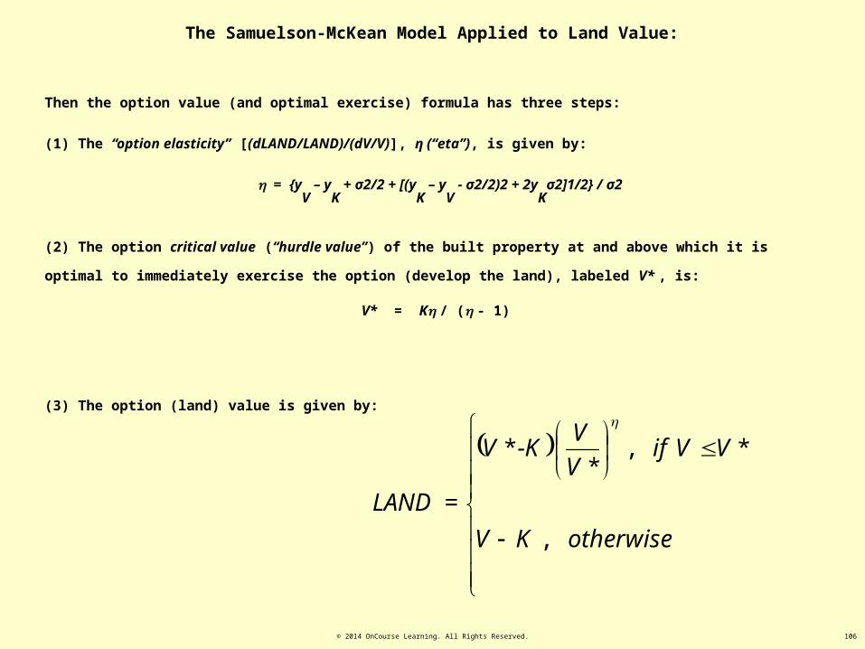
© 2014 OnCourse Learning. All Rights Reserved. 106
(3) The option (land) value is given by:
Then the option value (and optimal exercise) formula has three steps:
(1) The “option elasticity” [(dLAND/LAND)/(dV/V)], η (“eta”), is given by:
= {yV
– yK
+ σ2/2 + [(yK
– yV
- σ2/2)2 + 2yK
σ2]1/2} / σ2
(2) The option critical value (“hurdle value”) of the built property at and above which it is optimal to immediately exercise the option
(develop the land), labeled V* , is:
V* = K / ( - 1)
The Samuelson-McKean Model Applied to Land Value:
otherwiseKV
VVifV
V-KV
= LAND
,
*,*
*
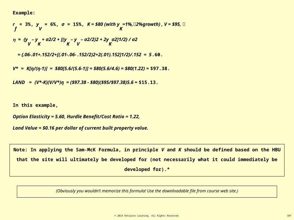
© 2014 OnCourse Learning. All Rights Reserved. 107
Example:
rf = 3%, y
V = 6%, σ = 15%, K = $80 (with y
K=1%,2%growth) , V = $95,
= {yV
– yK
+ σ2/2 + [(yK
– yV
– σ2/2)2 + 2yK
σ2]1/2} / σ2
= {.06-.01+.152/2+[(.01-.06- .152/2)2+2(.01).152]1/2}/.152 = 5.60.
V* = K[η/(η-1)] = $80[5.6/(5.6-1)] = $80(5.6/4.6) = $80(1.22) = $97.38.
LAND = (V*-K)(V/V*)η = ($97.38 - $80)($95/$97.38)5.6 = $15.13.
In this example,
Option Elasticity = 5.60, Hurdle Benefit/Cost Ratio = 1.22,
Land Value = $0.16 per dollar of current built property value.
(Obviously you wouldn’t memorize this formula! Use the downloadable file from course web site.)
Note: In applying the Sam-McK Formula, in principle V and K should be defined based on the HBU that the site will ultimately be
developed for (not necessarily what it could immediately be developed for).*

© 2014 OnCourse Learning. All Rights Reserved. 108
$0.00
$0.10
$0.20
$0.30
$0.40
$0.50
$0.60
$0.70
$0.00 $0.15 $0.30 $0.45 $0.60 $0.75 $0.90 $1.05 $1.20 $1.35 $1.50 $1.65
BUILT PROPERTY VALUE (V)
LAN
D (
OP
TIO
N)
VA
LUE
Option Value Option Value at Expiration
NPV of Construction
LandValue
V*=$1.28"Hurdle"
DevlptOptimal
Here is a picture of what the Samuelson-McKean Formula looks like:
Land value (LAND) is a monotonically increasing, convex function of the current HBU built property value (underlying asset value). Above the hurdle
benefit/cost (V/K) ratio, the option should already be exercised, and its value is simply V-K.
Parameters in above chart are: σ = 15%, yV
= 8%, yK
= 5%.

© 2014 OnCourse Learning. All Rights Reserved. 109
Both the option value, and the hurdle V/K ratio, are increasing functions of the volatility (σ) and decreasing functions of the payout
ratio (y).
$0.00
$0.10
$0.20
$0.30
$0.40
$0.50
$0.60
$0.70
$0.00 $0.15 $0.30 $0.45 $0.60 $0.75 $0.90 $1.05 $1.20 $1.35 $1.50 $1.65
BUILT PROPERTY VALUE (V)
LAN
D (
OP
TIO
N)
VA
LUE
(L)
Opt Val @ 15% Vol Opt Val @ 20% Vol Option Value at Expiration
V* =$1.28
V* = $1.44
The hurdle benefit/cost ratio, and the land value as a fraction of the construction cost, are independent of the scale of the site (in the
sense of the size of the land parcel, holding HBU density constant).
Assuming: yV
= 8%, yK
= 5%.
Exhibit 27-7
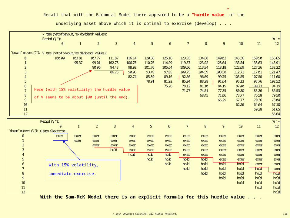
© 2014 OnCourse Learning. All Rights Reserved. 110
Recall that with the Binomial Model there appeared to be a “hurdle value” of the underlying asset above which it is optimal to
exercise (develop) . . .
With the Sam-McK Model there is an explicit formula for this hurdle value . . .
V tree (net of payout, "ex dividend" values):Period ("j "): "n " =
0 1 2 3 4 5 6 7 8 9 10 11 12
"down" moves ("i"): V tree (net of payout, "ex dividend" values):0 100.00 103.81 107.77 111.87 116.14 120.56 125.16 129.93 134.88 140.02 145.36 150.90 156.651 95.37 99.01 102.78 106.70 110.76 114.99 119.37 123.92 128.64 133.54 138.63 143.912 90.96 94.43 98.02 101.76 105.64 109.66 113.84 118.18 122.69 127.36 132.223 86.75 90.06 93.49 97.05 100.75 104.59 108.58 112.71 117.01 121.474 82.74 85.89 89.16 92.56 96.09 99.75 103.55 107.50 111.605 78.91 81.92 85.04 88.28 91.64 95.13 98.76 102.526 75.26 78.12 81.10 84.19 87.40 90.73 94.197 71.77 74.51 77.35 80.30 83.36 86.538 68.45 71.06 73.77 76.58 79.509 65.29 67.77 70.36 73.04
10 62.26 64.64 67.1011 59.38 61.6512 56.64
Period ("j "): "n " =0 1 2 3 4 5 6 7 8 9 10 11 12
"down" moves ("i"): Optimal exercise:0 exer exer exer exer exer exer exer exer exer exer exer exer exer1 exer exer exer exer exer exer exer exer exer exer exer exer2 exer exer exer exer exer exer exer exer exer exer exer3 hold exer exer exer exer exer exer exer exer exer4 hold hold hold exer exer exer exer exer exer5 hold hold hold hold exer exer exer exer6 hold hold hold hold hold exer exer7 hold hold hold hold hold exer8 hold hold hold hold hold9 hold hold hold hold
10 hold hold hold11 hold hold12 hold
With 15% volatility, immediate exercise.
Here (with 15% volatility) the hurdle value of V seems to be about
$90 (until the end).

© 2014 OnCourse Learning. All Rights Reserved. 111
The hurdle benefit/cost ratio:
(V*/K) = η / (η-1)
is an interesting measure in its own right.
It tells you how much greater the anticipated completed new built property value (including land) must be
than its construction cost (excluding land), in order for it to be optimal to stop waiting to develop, and
immediately begin (instantaneous) construction.
Expressing this in terms of the land value fraction of the total development project value at the time of optimal
development, the optimal land value fraction is given by the inverse of the elasticity:
11
1*
1*
*
V
K
V
KV
e.g., Elasticity = 3 Hurdle B/C Ratio = 1.5 Optimal Land Fraction = 33%.

© 2014 OnCourse Learning. All Rights Reserved. 112
Samuelson-McKean Implications for Optimal Development
As noted, the option elasticity also determines the hurdle benefit/cost ratio, V*/K, at which it is optimal to immediately
begin development whenever the current value of V and K equate to this ratio*:
1
*
K
V
The hurdle benefit/cost ratio is thus an inverse function of the option elasticity: larger elasticity means a lower hurdle
ratio.

© 2014 OnCourse Learning. All Rights Reserved. 113
Samuelson-McKean Implications for Optimal Development
Hurdle Ratio ( V* / K ) as a function of underlying asset volatility ( σ ):
With: yV
= 8%, yK
= 2%.
1.00
1.05
1.10
1.15
1.20
1.25
1.30
1.35
1.40
1.45
1.50
10%
11%
12%
13%
14%
15%
16%
17%
18%
19%
20%
21%
22%
23%
24%
25%
Underlying Asset Volatility ("sigma")
Hu
rdle
Ra
tio
( V
* /
K )

© 2014 OnCourse Learning. All Rights Reserved. 114
Samuelson-McKean Implications for Optimal Development
Hurdle Ratio ( V* / K ) as a function of underlying asset yield ( yV
):
With: σ = 15%, yK
= 2%.
1.00
1.20
1.40
1.60
1.80
2.00
2.20
2% 3% 4% 5% 6% 7% 8% 9% 10%
11%
12%
Underlying Asset Yield ("y(V)"))
Hu
rdle
Ra
tio
( V
* /
K )

© 2014 OnCourse Learning. All Rights Reserved. 115
Samuelson-McKean Implications for Optimal Development
Hurdle Ratio ( V* / K ) as a function of construction yield (yK
= rf – g
K ):
With: yV
= 8%, σ = 15%.
1.00
1.10
1.20
1.30
1.40
1.50
1.60
1.70
0% 1% 2% 3% 4% 5% 6% 7% 8% 9% 10%
Construction Yield ("y(K)")
Hu
rdle
Ra
tio
( V
* /
K )
© 2014 OnCourse Learning. All Rights Reserved. 116
The hurdle benefit/cost ratio (& optimal land fraction) is:
• Greater the more volatile is the built property market (i.e., the more uncertainty there is in the future value of built
properties):
• As long as you hold the option unexercised, greater volatility gives you greater potential upside outcomes you can take advantage of
while the option flexibility allows you to avoid the greater downside outcomes implied by the greater volatility.
• Uncertain and volatile property markets will dampen development, as developers wait until they can get built property values (based on
space market rents) sufficiently above the construction cost exclusive of land).
• Lower the greater is the current cash yield (akin to cap rate) being provided by built properties:
• You only start to get the net rent the property can generate when the building is complete, so the greater the current yield, the greater
the incentive to build sooner rather than later.
• Land value (site acquisition cost) will be a smaller fraction of total development cost (including construction) in locations where built
property values tend to grow slower (holding risk constant, lower “g” higher “y”, as g+y=r, recalling Ch.9).

© 2014 OnCourse Learning. All Rights Reserved. 117
Example:
In the U.S., land (site acquisition) is typically about 20% of the total development cost in most areas of the country, but often 50% in
major metropolises on the East and West Coast. Why?
Big East & West Coast Cities Rest of U.S.
Property Mkt Volatility (σ) 20% 15%
Property Payout Rate (y) 5% 8%
Big East & West Coast Cities
Rest of U.S.
LAND/V* @ V=V* (optimal dvlpt)
46% 22%
Then the Samuelson-McKean Formula gives the following difference in land value fraction of total developed property value at the
time of optimal development (based on the implied V*/K hurdle ratio):
Suppose rf = 5%, and property market volatility and payout rates differ as follows:

© 2014 OnCourse Learning. All Rights Reserved. 118
The option elasticity measure, η, is also interesting in its own right.
Prior to the point of optimal exercise (when the land is still optimally held undeveloped for speculation), the
elasticity tells the percentage change in land value resulting from a given percentage change in built property
value (for the type of property that would be the HBU of the land).
For a “live” option (below the hurdle ratio) the elasticity is:
• Independent of the size of the land parcel (for a given HBU density);
• Independent of the current value of the underlying asset (the state of the property market).*
• A decreasing function of the volatility in the property market.

© 2014 OnCourse Learning. All Rights Reserved. 119
The option elasticity relates the volatility (and risk) of the option (the undeveloped land investment) to the
volatility (and risk) of the underlying asset (the built property market for the HBU of the site).
Assuming riskless construction costs:
σLAND
= ησV ,
Where σLAND
is the volatility of the undeveloped land.
Since the option return is perfectly correlated with the underlying asset return, the option elasticity can
therefore also be used to relate the required expected investment return risk premium in undeveloped land to
that in the HBU built property market:
RPLAND
= ηRPV
.

© 2014 OnCourse Learning. All Rights Reserved. 120
Example:
Built property expected return rV
= 8%, Cash yield yV
= 6%
Riskfree interest rate = 4%, Built property RPV
= 4%.
Construction yield yK
= 2%.
(Which might be determined as the 4% riskfree rate minus a 2% likely construction cost growth rate: yK
= rf
– gK
= 4% - 2% = 2%.)
If built property volatility σ = 15%, then: (σ =.15, yV
=.06, yK
=.02)
η = 4.9.
Thus, RPLAND
= η(RPV
) = 4.9(4%) = 19.7%
Expected return (OCC) on land speculation investment =
rf + RP
LAND = 4% + 19.7% = 23.7%.
Based on the Samuelson-McKean assumptions, this required expected return for land speculation would hold no matter how big or small the land parcel
(for a given HBU density), or what the current state of the built property market is, as long as σ, y, rf , and RP
V remain the same. The Sam-McK Formula
is a “constant elasticity” formula.

© 2014 OnCourse Learning. All Rights Reserved. 121
Samuelson-McKean Implications for Land OCC
As noted, the option elasticity, η , gives the ratio of the land risk to the underlying asset risk, hence the ratio of the land to
underlying asset expected risk premium in the opportunity cost of capital (in the expected investment return):
][
][
V
C
RPE
RPE
We also noted that for a “live option” (not yet ripe for exercise) η is independent of both:
• Scale (value of V or of K ), and
• Current benefit cost ratio (amount of “operational leverage” in the construction project: V /
K
In fact, η is a function of only three variables: σ, yV
, and yK
.
This makes the option elasticity in the Samuelson-McKean Formula a very useful tool for understanding and quantifying
land investment risk and return requirements.
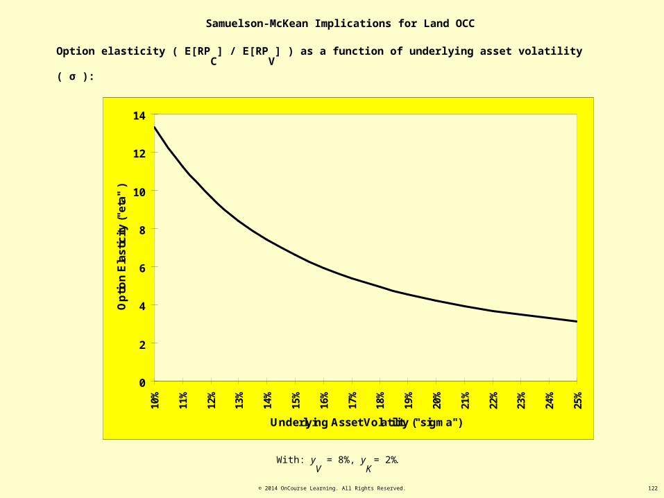
© 2014 OnCourse Learning. All Rights Reserved. 122
Samuelson-McKean Implications for Land OCC
Option elasticity ( E[RPC
] / E[RPV
] ) as a function of underlying asset volatility ( σ ):
With: yV
= 8%, yK
= 2%.
0
2
4
6
8
10
12
14
10%
11%
12%
13%
14%
15%
16%
17%
18%
19%
20%
21%
22%
23%
24%
25%
Underlying Asset Volatility ("sigma")
Op
tio
n E
las
tic
ity
("e
ta"
)

© 2014 OnCourse Learning. All Rights Reserved. 123
Option elasticity ( E[RPC
] / E[RPV
] ) as a function of underlying asset yield ( yV
):
With: σ = 15%, yK
= 2%.
0
2
4
6
8
10
12
2.0%
3.0%
4.0%
5.0%
6.0%
7.0%
8.0%
9.0%
10.0
%
11.0
%
12.0
%
Underlying Asset Yield ("y(V)")
Op
tio
n E
las
tic
ity
("e
ta"
)
Samuelson-McKean Implications for Land OCC

© 2014 OnCourse Learning. All Rights Reserved. 124
Option elasticity ( E[RPC
] / E[RPV
] ) as a function of construction yield (yK
= rf – g
K ):
With: yV
= 8%, σ = 15%.
Samuelson-McKean Implications for Land OCC
0
1
2
3
4
5
6
7
8
9
0.0%
1.0%
2.0%
3.0%
4.0%
5.0%
6.0%
7.0%
8.0%
9.0%
10.0
%
Construction Yield ("y(K)")
Op
tio
n E
las
tic
ity
("e
ta"
)
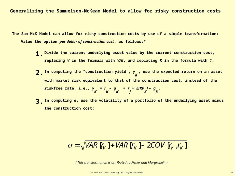
© 2014 OnCourse Learning. All Rights Reserved. 125
Generalizing the Samuelson-McKean Model to allow for risky construction costs
The Sam-McK Model can allow for risky construction costs by use of a simple transformation: Value the option per dollar of
construction cost, as follows:*
1. Divide the current underlying asset value by the current construction cost, replacing V in the formula with V/K,
and replacing K in the formula with 1.
2. In computing the “construction yield”, yK
, use the expected return on an asset with market risk equivalent to
that of the construction cost, instead of the riskfree rate. i.e., yK
= rK
– gK
= rf + E[RP
K] – g
K .
3. In computing σ, use the volatility of a portfolio of the underlying asset minus the construction cost:
],[2][][ KVKV rrCOVrVARrVAR
( This transformation is attributed to Fisher and Margrabe* .)

© 2014 OnCourse Learning. All Rights Reserved. 126
Summarizing up to now:
• The Binomial Model can handle:
• Finite-lived development options (rights expire at a specified future time), “American” or…
• “European” development options (construction prohibited prior to a given future point in time)
• The Samuelson-McKean Model can handle:
• The simple “Wait Option” for a perpetual “American” development option (typical “land value”
problem).
It remains for us to address two important considerations:
• Until now we have assumed instantaneous exercise: we need to consider the effect of construction time, aka “time
to build” .
• The “Phasing Option”, in which the project is broken into sequential phases rather than building it all at once

© 2014 OnCourse Learning. All Rights Reserved. 127
Appendix 27
27A.1.3: Time to Build
With non-instantaneous construction, when you exercise the option to build in state of the world i, j , you don’t get Vi,j
– Kj .
You get the PV of the completed project:
(Ei,j
[Vj+TC
])/(1+rV
)TC – Kj+TC
/(1+rf)TC
where TC is the number of periods it will take to complete construction.
In the Binomial Model, if you exercise the option at time 0 when the underlying asset has current observable value V0
, then
if the time to build is 1 period you will get:
KVfVfV
VV
fV y
K
y
V
r
K
r
VppV
r
K
r
yVdpyuVp
r
K
r
VEKVPV
1111
1
11
111
11
][][ 0011,11,0100110
11
If the time to build is 2 periods, you will get:
20
20
22
22,2
22,12,0
2
22
220
221111
112
11
][][
KVfVfV y
K
y
V
r
K
r
VpVppVp
r
K
r
VEKVPV
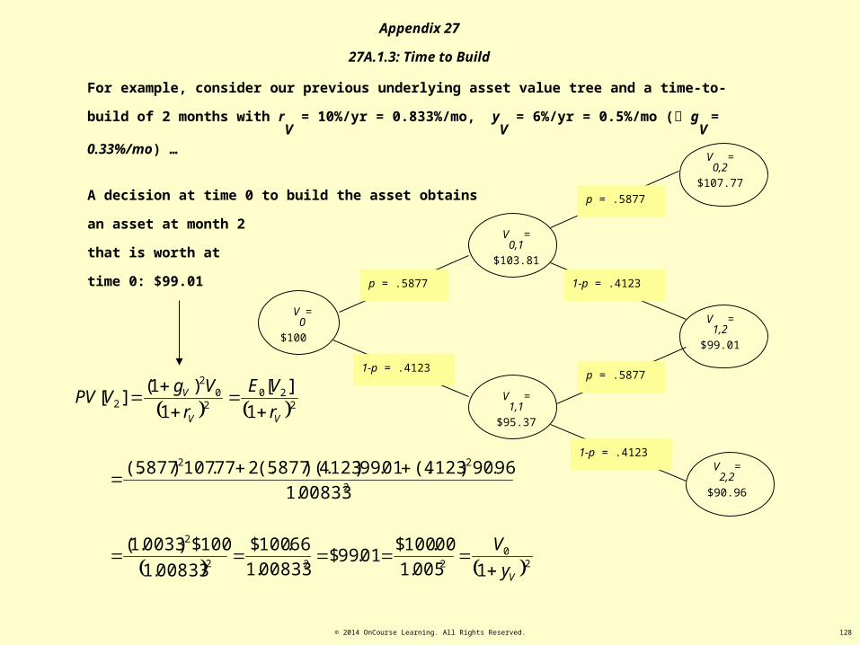
© 2014 OnCourse Learning. All Rights Reserved. 128
For example, consider our previous underlying asset value tree and a time-to-build of 2 months with rV
= 10%/yr
= 0.833%/mo, yV
= 6%/yr = 0.5%/mo ( gV
= 0.33%/mo) …
V1,2
=
$99.01
V0
=
$100
V0,1
=
$103.81
V1,1
=
$95.37
p = .5877
1-p = .4123
1-p = .4123
p = .5877
V2,2
=
$90.96
V0,2
=
$107.77
1-p = .4123
p = .5877A decision at time 0 to build the asset obtains an asset at month 2
that is worth at time 0:
$99.01
20
222
2
2
22
220
20
2
2
1005.1
00.100$01.99$
00833.1
66.100$
00833.1
100$)0033.1(
00833.1
96.90)4123(.01.99)4123)(.5877(.277.107)5877(.
1
][
1
)1(][
V
VV
V
y
V
r
VE
r
VgVPV
Appendix 27
27A.1.3: Time to Build

© 2014 OnCourse Learning. All Rights Reserved. 129
Summarizing:
To account for time to build in the option model:
• In any state i, j where the option could be exercised, replace the immediate exercise value
Vi,j
– Kj with the present value as of time j of the exercise value TC periods later (where
TC is the required construction time) : PVi,j
[Vj+TC
– Kj+TC
], as defined in the previous
slides.
• In the Samuelson-McKean Formula, replace the current value of the underlying asset,
Vij
, with: Vij
/ (1 + yV
)TC , and replace the exercise price Kj with K
j / (1 + y
K)TC .
Appendix 27
27A.1.3: Time to Build

© 2014 OnCourse Learning. All Rights Reserved. 130
The general effect of time-to-build is:
• The value of the option is reduced below what it otherwise would be.
• The expected time until optimal exercise is increased beyond what it otherwise would be
(hurdle value of Vt as measured by current observable price of pre-existing assets is
increased):
• Condition of optimal exercise, where “Vt” is current observable price of identical pre-existing
asset:
• η/(η-1) = (Vt /(1+y
V)TC ) / (K
t/(1+y
K)TC )
• Vt = K
t[η/(η-1)]((1+y
V)/(1+y
K))TC ,
• and normally: yV
> yK
.
Appendix 27
27A.1.3: Time to Build

© 2014 OnCourse Learning. All Rights Reserved. 131
Appendix 10C: Certainty Equivalence Discounting
• Review of traditional RADR DCF• Introduction to Certainty-Equivalence DCF• Example
Reference: Geltner-Miller et al 3e, Chapter 10 Appendix C (on the CD)
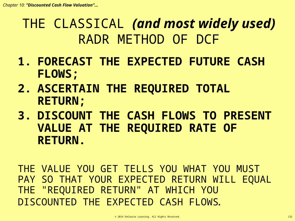
THE CLASSICAL (and most widely used) RADR METHOD OF DCF
1. FORECAST THE EXPECTED FUTURE CASH FLOWS;
2. ASCERTAIN THE REQUIRED TOTAL RETURN;
3. DISCOUNT THE CASH FLOWS TO PRESENT VALUE AT THE REQUIRED RATE OF RETURN.
THE VALUE YOU GET TELLS YOU WHAT YOU MUST PAY SO THAT YOUR EXPECTED RETURN WILL EQUAL THE "REQUIRED RETURN" AT WHICH YOU DISCOUNTED THE EXPECTED CASH FLOWS.
© 2014 OnCourse Learning. All Rights Reserved. 132
Chapter 10: “Discounted Cash Flow Valuation”…

TT
TT
rE
CFE
rE
CFE
rE
CFE
rE
CFEV
][1
][
][1
][
][1
][
][1
][
0
01
0
102
0
20
0
100
where:
CFt = Net cash flow generated by the property in period “t”; Vt = Property value at the end of period “t”; E0[r] = Expected average multi-period return (per period) as of time “zero” (the present), also known as the “going-in IRR”; T = The terminal period in the expected investment holding period, such that CFT would include the re-sale value of the property at that time (VT), in addition to normal operating cash flow.
© 2014 OnCourse Learning. All Rights Reserved. 133
Chapter 10: “Discounted Cash Flow Valuation”…
Match the discount rate to the risk. . .
r = rf + RP
Disc.Rate = Riskfree Rate + Risk Premium
(Riskfree Rate = US T-Bill Yield.)
© 2014 OnCourse Learning. All Rights Reserved. 134
Chapter 10: “Discounted Cash Flow Valuation”…

© 2014 OnCourse Learning. All Rights Reserved. 135
Appendix 10C: “Certainty-Equivalent Valuation”…
Consider the fundamental element of our valuation model:
][1
][)(
0
101
VrE
VEVPV
Accounts for both time and risk in the discount rate in the denominator, as , where rf is
riskless and accounts for the time value of money, and RPV
is the market’s required risk premium in the
expected return for the investment (ex ante).
][0 VfV RPErrE
Manipulate this formula so that the denominator purely reflects the time value of money (the discounting is done
risklessly) and the risk is completely and purely accounted for in the numerator, by reducing the cash flow
amount in the numerator to a “Certainty Equivalent Value” . . .

© 2014 OnCourse Learning. All Rights Reserved. 136
][1
][
][1
][)( 10
0
101
VfV RPEr
VE
rE
VEVPV
f
V
r
VPVRPEVEVPV
1
)(][][)( 110
1
)(][][)(1 1101 VPVRPEVEVPVr Vf
][)(][)(1 1011 VEVPVRPEVPVr Vf
][)(][1 101 VEVPVRPEr Vf
A little algebra . . .
Appendix 10C: “Certainty-Equivalent Valuation”…
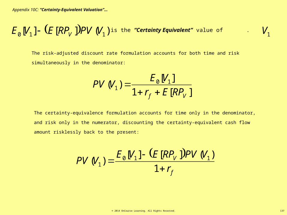
© 2014 OnCourse Learning. All Rights Reserved. 137
][1
][)( 10
1Vf RPEr
VEVPV
f
V
r
VPVRPEVEVPV
1
)(][][)( 110
1
)(][][ 110 VPVRPEVE V is the “Certainty Equivalent” value of . 1V
The risk-adjusted discount rate formulation accounts for both time and risk simultaneously in the
denominator:
The certainty-equivalence formulation accounts for time only in the denominator, and risk only in the
numerator, discounting the certainty-equivalent cash flow amount risklessly back to the present:
Appendix 10C: “Certainty-Equivalent Valuation”…

© 2014 OnCourse Learning. All Rights Reserved. 138
][1
][)( 10
1Vf RPEr
VEVPV
f
V
r
VPVRPEVEVPV
1
)(][][)( 110
1
)(][][ 110 VPVRPEVE V is the “Certainty Equivalent” value of . 1V
The risk-adjusted discount rate formulation accounts for both time and risk simultaneously in the
denominator:
The certainty-equivalence formulation accounts for time only in the denominator, and risk only in the
numerator, discounting the certainty-equivalent cash flow amount risklessly back to the present:
Appendix 10C: “Certainty-Equivalent Valuation”…
Risk premium (in %)
Risk discount (in $), aka
“Haircut”

© 2014 OnCourse Learning. All Rights Reserved. 139
)(][][ 110 VPVRPEVE V
The investment market is indifferent between a claim on the actual risky
amount of V1
one period in the future (with the actual amount of risk
involved in that), versus a claim on the lesser amount of:
one period in the future with no risk at all.
The “haircutted” value is called the “certainty-equivalence value”, labeled “CEQ”:
Appendix 10C: “Certainty-Equivalent Valuation”…
)(][][)( 11010 VPVRPEVEVCEQ V

© 2014 OnCourse Learning. All Rights Reserved. 140
Why do we care about this? . . .
The certainty-equivalent approach is more general, can be applied in situations
where RADR discounting can’t be applied, including options valuation and other
derivatives valuations (e.g., swaps, forwards, futures).
Consider a simple example . . .
Appendix 10C: “Certainty-Equivalent Valuation”…
Typically, CEQ discounting useful if:
• Risk does not accumulate at a constant rate over time (i.e., there is no single correct OCC).
• PV=0 even though future cash flow expectations are not zero (as with futures contracts)
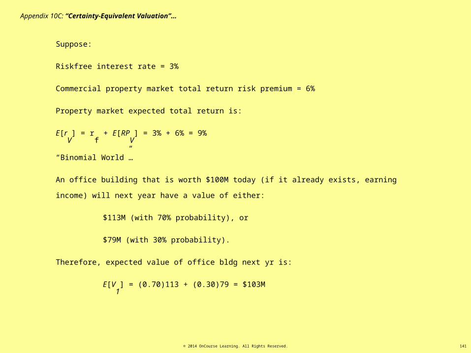
© 2014 OnCourse Learning. All Rights Reserved. 141
Suppose:
Riskfree interest rate = 3%
Commercial property market total return risk premium = 6%
Property market expected total return is:
E[rV
] = rf + E[RP
V] = 3% + 6% = 9%
“Binomial World”…
An office building that is worth $100M today (if it already exists, earning income) will next year have a
value of either:
$113M (with 70% probability), or
$79M (with 30% probability).
Therefore, expected value of office bldg next yr is:
E[V1
] = (0.70)113 + (0.30)79 = $103M
Appendix 10C: “Certainty-Equivalent Valuation”…
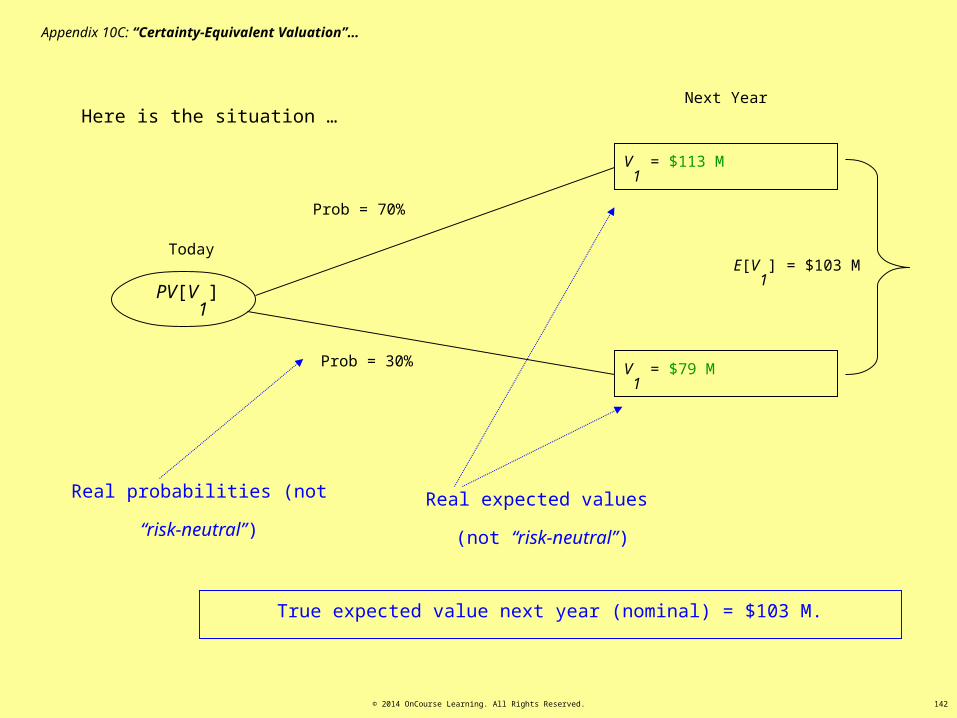
© 2014 OnCourse Learning. All Rights Reserved. 142
V1
= $113 M
V1
= $79 M
Prob = 70%
Prob = 30%
PV[V1
]
Here is the situation …
Today
Next Year
Appendix 10C: “Certainty-Equivalent Valuation”…
Real probabilities (not “risk-
neutral”)
Real expected values
(not “risk-neutral”)
True expected value next year (nominal) = $103 M.
E[V1
] = $103 M

© 2014 OnCourse Learning. All Rights Reserved. 143
MRPEr
VEVPV
Vf
94$09.1
103$
%6%31
79)$30(.113)$70(.
][1
][][ 10
1
Risk-adjusted discount rate valuation:
Mr
VPVRPEVE
r
VCEQVPV
f
V
f
94$03.1
97$
%31
94)$06(.103$
1
][][][
1
][][ 11010
1
Certainty-equivalent valuation:
$97 is the certainty-equivalent value of V1
whose expected value is $103.
How much is the forward claim on the office building worth today? . . .
If we know rf and either E[RP
V] or PV[V
1] then we can derive above.
Thus, easy to apply RADR discounting to underlying asset (due to transparency in market for trading such built properties).

© 2014 OnCourse Learning. All Rights Reserved. 144
MRPEr
VEVPV
Vf
94$09.1
103$
%6%31
79)$30(.113)$70(.
][1
][][ 10
1
Mr
VPVRPEVE
r
VCEQVPV
f
V
f
94$03.1
97$
%31
94)$06(.103$
1
][][][
1
][][ 11010
1
How much is the forward claim on the office building worth today? . . .
If we know rf and either E[RP
V] or PV[V
1] then we can derive above.
Even if we just know V0
(current value of pre-existing “twin” building) and yV
(cash payout rate, or income yield, of such building)…
PV[V1
] = (1 + gV
)V0
/ (1 + rV
) = V0
/ (1 + yV
) ,
e.g., with 6% “caprate”, $94 = $103 / 1.09 = $100 / 1.06.
This is due to relationship between rV
, gV
, & yV
:
(1 + rV
) / (1 + yV
) = (1 + gV
) rV
≈ yV
+ gV
(This is an “accounting relationship”: Holds by definition.)
Thus, easy to apply RADR discounting to underlying asset (due to transparency in market for trading such built properties).

© 2014 OnCourse Learning. All Rights Reserved. 145
Now suppose the office building does not exist yet,
but we could build it in 1 year
by paying $90M of construction cost next year. (Construction is instantaneous: We can decide
next year whether to build or not.)
Suppose our option to build this project expires in 1 year: We either build then or we lose the
right to ever build.
Suppose market for such options is thin, lacks transparency, so we cannot directly observe
value of option or of relevant E[RP] in discount rate…
How much is this option worth?
Appendix 10C: “Certainty-Equivalent Valuation”…
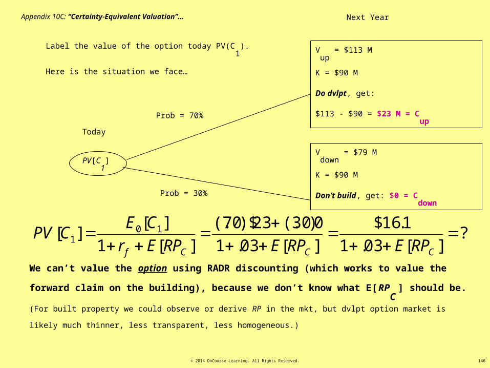
© 2014 OnCourse Learning. All Rights Reserved. 146
Label the value of the option today PV(C1
).
Here is the situation we face…
Vup
= $113 M
K = $90 M
Do dvlpt, get:
$113 - $90 = $23 M = Cup
Vdown
= $79 M
K = $90 M
Don’t build, get: $0 = Cdown
Prob = 70%
Prob = 30%
PV[C1
]
Today
Next YearAppendix 10C: “Certainty-Equivalent Valuation”…
?][03.1
1.16$
][03.1
0)30(.23)$70(.
][1
][][ 10
1
CCCf RPERPERPEr
CECPV
We can’t value the option using RADR discounting (which works to value the forward claim on the
building), because we don’t know what E[RPC
] should be. (For built property we could observe or derive RP
in the mkt, but dvlpt option market is likely much thinner, less transparent, less homogeneous.)

© 2
014
OnC
ours
e Le
arni
ng. A
ll Ri
ghts
Res
erve
d.
147
Risk
E[r]
rf = 3%
34%
9%
Built Property
37% range
Devlpt Option
192% range
E[RP]
Invoke “linear pricing” principle (aka “Law of One Price”):
• Same “Price of Risk” must apply to all assets at a given time.
• Same expected return risk premium per unit of risk (ex ante).
• Otherwise, “not fair” (people will trade until “One Price” holds).
Among “derivative” assets, relative risk can be measured by volatility (or return outcome spread range) ratio between the
derivative & the underlying asset. “Derivatives” are assets that are perfectly correlated: derivative outcome depends entirely on
underlying outcome.
(We don’t know this yet.)
(We don’t know this yet.)

© 2014 OnCourse Learning. All Rights Reserved. 148
162.0
%36
%6
%)16(%)20(
%3%9
%%
][
][$$
][
94$79$113$
%3%9
11111
downupV
downupV
VV
RPE
VPVVV
RPE
Price of risk in the “underlying asset” (the completed built office bldg – what you can get by exercising
the development option) = Risk Premium / Risk (spread)…
Appendix 10C: “Certainty-Equivalent Valuation”…
7.3$162.00$23$162.0$$][][
,$$
][][
][$$
][162.0
111
11
1
111
downupC
downupC
downupC
CCCPVRPE
CC
CPVRPE
CPVCC
RPE
Therefore, price of risk must be the same in the derivative asset, the development option:
Now we have all we need to apply the certainty-equivalence discounting formula to value the option…

© 2014 OnCourse Learning. All Rights Reserved. 149
Now we have all we need to apply the certainty-equivalence discounting formula to value the option:
Appendix 10C: “Certainty-Equivalent Valuation”…
M
r
CPVRPECE
r
CCEQCPV
f
C
f
12$03.1
4.12$
%31
7.3$1.16$
%31
7.3$0)3(.23)$7(.
1
][][][
1
][)( 11010
1
Risk
E[r]
rf = 3%
34%
9%
Built Property
37% range
Devlpt Option
192% range
E[RP]

150
%31%10312$
1.16$][
,][%31
1.16$
][1
][12$][ 10
1
C
CCf
RPE
RPERPEr
CECPV
Having computed (derived ) PV[C1
], we can now back out the implied E[RPC
] and RADR for the
option…
Which implies that the option has 31/6 = 5.2 times the investment risk that the built office property
has, as:
E[RPC
] = 31% = (5.2)*6% = (5.2)*E[RPV
].
However, if we didn’t already know the option’s risk premium (31%), or hadn’t already done the certainty-equivalent valuation, we wouldn’t be able to use the RADR
method of DCF valuation.
Appendix 10C: “Certainty-Equivalent Valuation”…
MRPEr
CECPV
Cf
12$34.1
1.16$
31.03.1
0)30(.23)$70(.
][1
][][ 10
1
© 2
014
OnC
ours
e Le
arni
ng. A
ll Ri
ghts
Res
erve
d.

151
Risk
E[r]
rf = 3%
34%
9%
Built Property
37% range
Devlpt Option
192% range
E[RP]
Invoke “linear pricing” principle (aka “Law of One Price”):
• Same “Price of Risk” must apply to all assets at a given time.
• Same expected return risk premium per unit of risk (ex ante).
• Otherwise, “not fair” (people will trade until “One Price” holds).
Among “derivative” assets, relative risk can be measured by volatility (or return outcome spread range) ratio between the
derivative & the underlying asset…
(Now we know this.)
(Now we can compute this.)
© 2
014
OnC
ours
e Le
arni
ng. A
ll Ri
ghts
Res
erve
d.
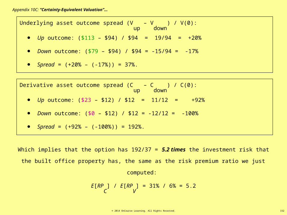
© 2014 OnCourse Learning. All Rights Reserved. 152
Underlying asset outcome spread (Vup
– Vdown
) / V(0):
• Up outcome: ($113 – $94) / $94 = 19/94 = +20%
• Down outcome: ($79 – $94) / $94 = -15/94 = -17%
• Spread = (+20% – (-17%)) = 37%.
Which implies that the option has 192/37 = 5.2 times the investment risk that the built office property
has, the same as the risk premium ratio we just computed:
E[RPC
] / E[RPV
] = 31% / 6% = 5.2
Appendix 10C: “Certainty-Equivalent Valuation”…
Derivative asset outcome spread (Cup
– Cdown
) / C(0):
• Up outcome: ($23 – $12) / $12 = 11/12 = +92%
• Down outcome: ($0 – $12) / $12 = -12/12 = -100%
• Spread = (+92% – (-100%)) = 192%.

© 2014 OnCourse Learning. All Rights Reserved. 153
Risk
E[r]
rf = 3%
34%
9%
Built Property
37% range
Devlpt Option
192% range
E[RP]
If this relationship does not hold, then there are “super-normal” (disequilibrium) profits (expected
returns) to be made somewhere, and correspondingly “sub-normal” profits elsewhere, across the
markets for: Land, Built Property, and Bonds (“riskless” CFs).
The “Law of One Price”…

© 2014 OnCourse Learning. All Rights Reserved. 154
17.0%36
%6
%)16(%)20(
%3%9
%%][$$94$79$113$
%3%9
11111
downupV
downupV
VV
RP
VPVVV
RP
Fundamentally, what we are doing here is making sure that the expected return risk premium per unit of risk is the same
between an investment in the development option, and an investment in already-build (stabilized) property. For example, for
stabilized property:
Appendix 10C: “Certainty-Equivalent Valuation”…
17.0%190
%31
%)100(%)90(
%3%34
%%][$$12$0$23$
%3%34
11111
downupC
downupC
CC
RP
CPVCC
RP
For the development option:
Thus, this procedure for the valuation of the development option is equivalent to a cross-market equilibrium condition: that the
expected return risk premium per unit of risk (or the “risk-adjusted return”) presented by the investments should be the same
between the market for development options and the market for stabilized built property. Otherwise, investors will buy one type
of asset and sell the other type until prices equilibrate the risk-adjusted returns across the two markets.

© 2014 OnCourse Learning. All Rights Reserved. 155
General formula to value derivative “C” based on underlying asset “V”…
12$03.1
4.12$
03.1
7.3$1.16$03.1
162.23$1.16$
03.1%36%6
23$1.16$
%3194/7994/113
%3%90$23$0)30(.23)$70(.
][
:.,.
1
%%
][][
][
1
10
1
CPV
exampleouringe
r
VV
rrECCCE
CPVf
downup
fVdownup
Appendix 10C: “Certainty-Equivalent Valuation”…

© 2014 OnCourse Learning. All Rights Reserved. 156
12$34.1
1.16$
%31%31
0)$30(.23)$70(.
][1
][ 100
Cf RPEr
CEC
The equivalent valuation using the risk-adjusted discount rate approach is:
Which implies that the option has 31/6 = 5.2 times the investment risk that the office building has (and that the
stock market has), as:
RPC
= 31% = 5.2*6% = 5.2*RPV
(= 5.2*RPS
).
However, if we didn’t already know the option’s risk premium (31%), or hadn’t already done the certainty-equivalent
approach, we wouldn’t be able to use the risk-adjusted discount rate approach.
The certainty-equivalent approach does not require prior knowledge of RPC
. It only requires knowledge of Cup
,
Cdown
, and the “up” probability (70% in our example).
This makes the certainty-equivalent approach very useful for option valuation. Most development projects are
essentially “options”.
Appendix 10C: “Certainty-Equivalent Valuation”…
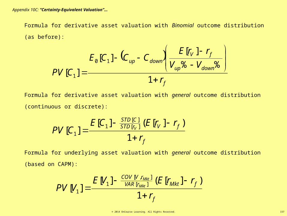
© 2014 OnCourse Learning. All Rights Reserved. 157
Formula for derivative asset valuation with Binomial outcome distribution (as before):
f
downup
fVdownup
r
VV
rrECCCE
CPV
1
%%
][][
][10
1
Appendix 10C: “Certainty-Equivalent Valuation”…
Formula for derivative asset valuation with general outcome distribution (continuous or discrete):
f
fVrSTDCSTD
r
rrECECPV V
1
)][(][][ ][
][1
1
Formula for underlying asset valuation with general outcome distribution (based on CAPM):
f
fMktrVARrVCOV
r
rrEVEVPV Mkt
Mkt
1
)][(][][ ][
],[1
1
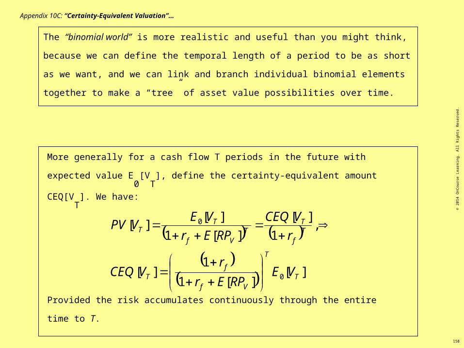
158
The “binomial world” is more realistic and useful than you might think, because we can
define the temporal length of a period to be as short as we want, and we can link and branch
individual binomial elements together to make a “tree” of asset value possibilities over time.
More generally for a cash flow T periods in the future with expected value E0
[VT
],
define the certainty-equivalent amount CEQ[VT
]. We have:
][][1
1][
,1
][
][1
][][
0
0
T
T
Vf
fT
Tf
TT
Vf
TT
VERPEr
rVCEQ
r
VCEQ
RPEr
VEVPV
Appendix 10C: “Certainty-Equivalent Valuation”…
Provided the risk accumulates continuously through the entire time to T.
© 2
014
OnC
ours
e Le
arni
ng. A
ll Ri
ghts
Res
erve
d.

© 2014 OnCourse Learning. All Rights Reserved. 159
Intuition in the CEQ formula:
The certainty equivalent value next year is the downward adjusted value of the risky expected value for which the investment market would be
indifferent between that value and a riskfree bond value of the same amount…
f
downup
fVdownup
f r
VV
rrECCCE
r
CCEQC
1
%%
][][
1
][10
100
The certainty equivalent value next year is the expected value minus a risk discount.
%%
][
downup
fVdownup VV
rrECC
The risk discount consists of the amount of risk in the next year’s value as
indicated by the range in the possible outcomes times…
times the market price of risk (for same “type”
of risk, e.g., office building*)
%%
][
downup
fV
VV
rrE
The market price of risk is the market expected return risk premium per unit of return risk for the same asset, the ratio of…
the market expected return risk premium divided by
the range in the corresponding return possible
outcomes.
*dvlpt option is perfectly
correlated with building

© 2014 OnCourse Learning. All Rights Reserved. 160
f
downup
fMktdownup
r
MktMkt
rrECCCE
C
1
%%
][][ 10
0
f
downup
fVdownup
r
VV
rrECCCE
C
1
%%
][][ 10
0
Technical aside
The astute student will have observed that there appears to be a slight difference between the certainty-equivalent valuation
formula presented in the Chapter 10 lecture notes:
And the one presented here:
(1)
(2)
Formula (1) assumes there is a “Market Portfolio”, and either that the option is perfectly correlated with that portfolio, or
else that the CAPM applies and the “up” and “down” movements considered in the formula are only those components that
are perfectly correlated with the “up” and “down” movements of the Market. Formula (2) is a more general expression.
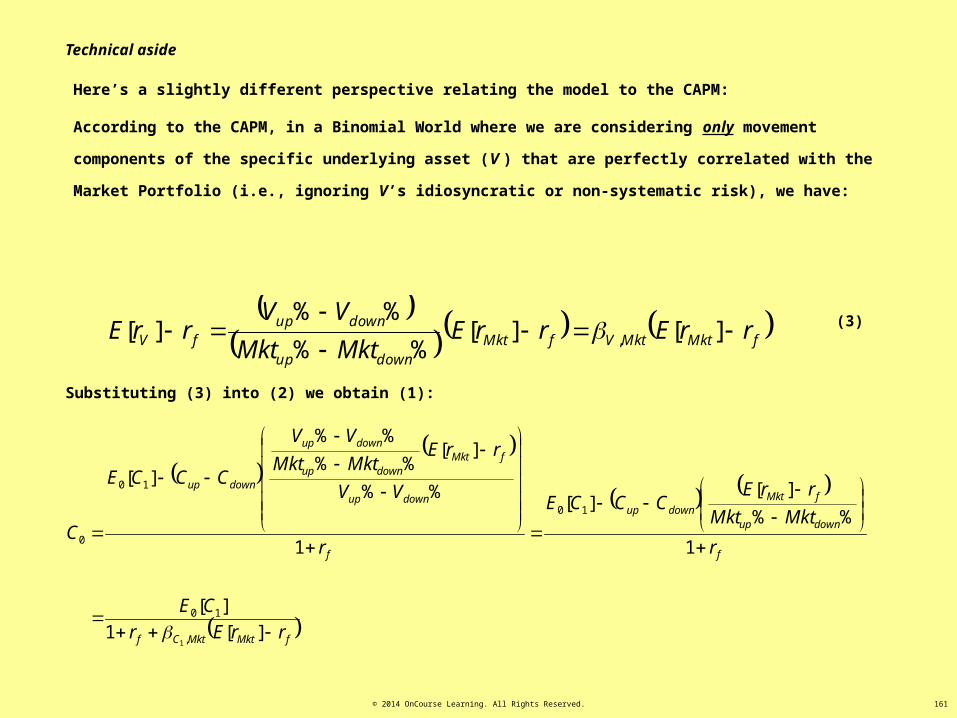
© 2014 OnCourse Learning. All Rights Reserved. 161
Technical aside
Here’s a slightly different perspective relating the model to the CAPM:
According to the CAPM, in a Binomial World where we are considering only movement components of the specific
underlying asset (V ) that are perfectly correlated with the Market Portfolio (i.e., ignoring V’s idiosyncratic or non-
systematic risk), we have:
fMktMktVfMkt
downup
downupfV rrErrE
MktMkt
VVrrE
][][%%
%%][ ,
Substituting (3) into (2) we obtain (1):
(3)
fMktMktCf
f
downup
fMktdownup
f
downup
fMktdownup
downup
downup
rrEr
CE
r
MktMkt
rrECCCE
r
VV
rrEMktMkt
VV
CCCE
C
][1
][
1
%%
][][
1
%%
][%%
%%
][
,
10
10
10
0
1

© 2014 OnCourse Learning. All Rights Reserved. 162
][
],[""
%
%
][
][
Mkt
MktV
Mkt
V
rVAR
rrCOVBeta
returninriskMkt
returninriskV
RPE
RPE
In the “CAPM”:
Recall this digression from our Ch.10 lecture on certainty-equivalent valuation
Three asides (see notes for further explanation)
The “binomial world” is much more realistic and useful than you might think, in part because we can define the temporal length of a
period to be as short as we want, and we can link and branch individual binomial elements together to make a “tree” of asset value
possibilities over time.
, Thus:
)][(1][
1)][(][
],[][1)][(][
10
1100100
fMktf
ffMktMkt
MktffMkt
rrErVE
rrrErVAR
rVCOVVErVrrEVEV
More generally for a cash flow T periods in the future with expected value E0
[VT
], define the certainty-equivalent amount CEQ[VT
]. We have:
][][1
1][,
1
][
][1
][0
00 T
T
Vf
fTT
f
TT
Vf
T VERPEr
rVCEQ
r
VCEQ
RPEr
VEV