ＬｅｃｔｕｒｅＬｅｃｔｕｒｅ 11

Describing DataDescribing Data

©

Histogram and frequency Histogram and frequency tabletable

Example

Visualizing your clients’ age range using a histogram.

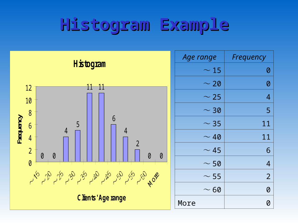
Histogram ExampleHistogram Example

Histogram

0 0

45

11 11

6

4

2

0 00

2

4

6

8

10

12

Clients' Age range

Freq

uenc

y

Age range Frequency

～ 15 0

～ 20 0

～ 25 4

～ 30 5

～ 35 11

～ 40 11

～ 45 6

～ 50 4

～ 55 2

～ 60 0

More 0

From the histogram, we can From the histogram, we can learn thatlearn that

Clients of age between 31~35 and 36~40 are the primary clients.

It is important to maintain the

satisfaction of these clients.

Provide new services for other age ranges to increase client base.

Making Histogram and Making Histogram and Frequency TableFrequency Table

Open the data “Clients list” which is stored in our Applied Stat Folder. This is the data for the histogram shown in the previous slides.

Numerical measures of data Numerical measures of data summary (I)summary (I)

Difference between Population and Sample

Mean (Average) Median

Difference between Difference between Population and SamplePopulation and Sample

PopulationPopulationA populationpopulation is the complete set of all items in which an investigator is interested.

Examples of Examples of PopulationsPopulations

Names of all registered voters in the United States.

Incomes of all families living in Daytona Beach.

Grade point averages of all the students in your university.

A major objective of statistics is to make an inference about the population. For example “What is the average income of all families living in Daytona Beach?”

Often, collecting the data for the population is costly or impossible. Therefore, we often collect data for only a part of the population. Such data is called a “Sample”.

A SampleA Sample

SampleSampleA samplesample is an observed subset of population values.

Numerical measure of Numerical measure of summarizing data summarizing data

1-1 Mean (Average)1-1 Mean (Average)

How to compute the mean (average) Understanding the mathematical

notation of the mean (average) Cautionary notes for the use of the

mean

1-2 How to compute the 1-2 How to compute the meanmean

Sum all the data, then divide it by the number of observations.

We use the term “sample size” to mean the number of observations.

1-3 Computing the mean: an 1-3 Computing the mean: an exampleexample

Client ID Age

1 49

2 37

3 48

4 46

5 37

•This is a sample data of the ages of your business clients. Compute the mean age of your clients in this sample.

•Note that this is a typical data format that we will encounter in this course. It has the observation id (Client ID), and the value of the variable of interest (age) for each observation.

2-1 Understanding the 2-1 Understanding the mathematical notation of the mathematical notation of the

meanmeanObservation

id Variable X

1 x1

2 x2

3 x3

.

...

n xn

This is one of the most common format of data that we deal with. In the first column, we have the observation id, and the second column has the value for each observation. (Often observation id is omitted)

In the previous example, variable X is the age of the clients. Then observation id =1 means that this is the first customer in your customer list, and x1 is the age of the customer.

2-2 Understanding the 2-2 Understanding the mathematical notation of the mathematical notation of the

meanmean

Observation id Variable X

1 x1

2 x2

3 x3

.

...

n xn

n

x

n

xxxX

n

ii

n

121

n

iix

1

When a data set is given in this format, the sample mean of the variable X, denoted by ,is given byX

The notation, is the

summation notation. This is simply the sum from x1 to xn

2-3 Sample Mean and 2-3 Sample Mean and Population MeanPopulation Mean

Most often we use a sample data. For example, if we want to know the popularity rating of the current government, we may use data from 10,000 interviews. This is just a part of the whole voting population.

Though not often, we may have the data from the whole population.

2-4 Sample Mean and 2-4 Sample Mean and Population MeanPopulation Mean

Later, it will become convenient to distinguish sample mean and population mean. Thus we will use different notations for the sample mean and the population mean.

2-5 Notations for the sample 2-5 Notations for the sample mean and the population mean and the population

meanmean

N

x

N

xxx

N

ii

N

121

n

x

n

xxxX

n

ii

n

121

For a sample mean, we use the following notation

For the population mean, we use μ. We also use upper case N to denote the population size.

3-1 Cautionary note3-1 Cautionary note

: Mean (average) is not necessarily the “center of the data”

3-2 Example3-2 Example “The average Japanese household

savings in year 2005 is ￥ 17,280,000”

This data may make you feel “well, if I do not have this much savings, I am not normal”

Now, take a look at the histogram of the household savings in the next slide.

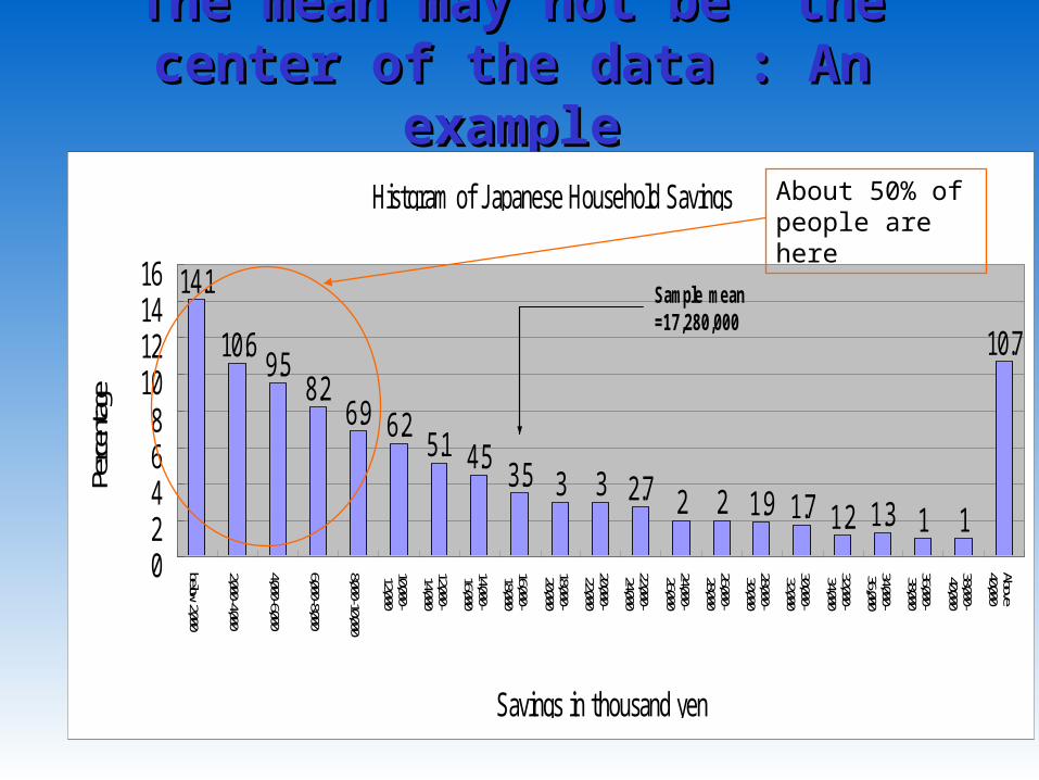
The mean may not be “the The mean may not be “the center of the data”: An center of the data”: An

exampleexampleHistgram of J apanese Household Savings

14.1

10.69.5

8.26.9 6.2

5.1 4.5 3.5 3 3 2.7 2 2 1.9 1.7 1.2 1.3 1 1

10.7

02468

10121416

below 2,000

2,000-4,000

4,000-6,000

6,000-8,000

8,000-10,000

10,000-12,000

12,000-14,000

14,000-16,000

16,000-18,000

18,000-20,000

20,000-22,000

22,000-24,000

24,000-26,000

26,000-28,000

28,000-30,000

30,000-32,000

32,000-34,000

34,000-36,,000

36,000-38,000

38,000-40,000

Above40,000

Savings in thousand yen

Perce

ntage

Sample mean=17,280,000

About 50% of people are here

One may think that the average is the “normal household”. However, you can see that a lot of households have savings much less than the average. The average savings is very high because a few households have huge savings.

In such case, “median” can give you a better sense of a “normal household”. The definition of the median is given in the next slide.

4-1 Median4-1 Median

Sort the data in an ascending order. Then the median is the value in the middle (middle observation)

When the number of observations is an even number, then there is no “middle observation”. In such case, take the average of the two middle numbers

4-2 Median Exercise4-2 Median Exercise

Open the file “ Computation of median A”. This data contains the age of a company’s clients. Find the median age of this sample

Open the file “Computation of median B”. This data contains the revenue of bag sales. Find the median of this sample.

Japanese household savings Japanese household savings revisitedrevisited

Histgram of J apanese Household Savings

14.1

10.69.5

8.26.9 6.2

5.1 4.5 3.5 3 3 2.7 2 2 1.9 1.7 1.2 1.3 1 1

10.7

02468

10121416

below 2,000

2,000-4,000

4,000-6,000

6,000-8,000

8,000-10,000

10,000-12,000

12,000-14,000

14,000-16,000

16,000-18,000

18,000-20,000

20,000-22,000

22,000-24,000

24,000-26,000

26,000-28,000

28,000-30,000

30,000-32,000

32,000-34,000

34,000-36,000

36,000-38,000

38,000-40,000

Above 40,000

Savings in thousand yen

Perce

ntage

Sample Average=17,280,000

Median =10,520,000

Corresponding chaptersCorresponding chapters

This lecture note covers the following topics of the textbook:

1.2 Sampling 3.1 Arithmetic Mean, Median