- 1 -

corresponding author : e-mail :alain.bosseboeuf@ief.u-psud.fr ; fax : (33) 1 69 15 40 00

3D measurement of micromechanical devices vibrationmode shapes by stroboscopic microscopic interferometry

S. Petitgrand, R. Yahiaoui, K. Danaie, A. Bosseboeuf*, J.P.Gilles

Institut d'Electronique Fondamentale, UMR CNRS 8622, Université Paris XI, Bât. 220F-91405 Orsay Cedex, France

Abstract :

Microscopic interferometry is a powerful technique for the static and dynamic characterization ofmicromechanical devices. In this paper we emphasize its capabilities for 3D vibration mode shapesprofiling of Al cantilever microbeams and Cr micromachined membranes. It is demonstrated thattime-resolved measurements up to 800 kHz can be performed with a lateral resolution in themicrometer range and a detection limit of 3-5 nm. In addition, with reduced image sizes (256x256),quasi real time (150-500ms) visualisation of the vibration mode 3D profiles becomes possible.These performances were obtained by using stroboscopic illumination with an array ofsuperluminescent LED and an optimised automatic Fast Fourier Transform phase demodulation ofthe interferograms. The results are compared with theoretical shapes of the vibration modes andwith point measurements of the vibration spectra.

Keywords : Vibrometry, Stroboscopic, Interferometry, MEMS, mechanical properties

- 2 -

I. Introduction

Optical measurement of the vibration spectra of micromechanical devices is a common method for

the characterization of the mechanical properties of thin films [1-9]. From the resonant frequencies

of cantilever microbeams [1-3], microbridges [4-7] or membranes [8,9] made in the material under

investigation, the film Young’s modulus and mean residual stress may be evaluated. Air damping,

which is the predominant effect at atmospheric pressure, can be characterized from the quality

factors of the resonances and/or the shifts of their frequency with respect to their value in vacuum.

[10]. Aging of the microdevices can be determined from the quality factors and frequency

variations of the resonances as function of time or annealing [4]. All these characterisations need an

unambiguous identification of the resonant peaks in the vibration spectra. The main resonant

frequencies of microbeams corresponding to flexural vibration modes can generally be identified

easily. For membranes or microbridges with internal residual stress, the vibration main modes order

may differ or not from that of unstressed microdevices according to the value and sign of the stress

value [6,7]. This makes uncertain the identification of the resonant peaks from a single vibration

spectrum only. Membrane vibration spectra are particularly difficult to interpret because they

contain numerous low quality factor resonances which correspond to complex vibration mode

shapes [8,9]. For such stressed elementary microdevices and for more complex

Micro(Opto)ElectroMechanical Systems (M(O)EMS), it is clear that a single spectrum is generally

not sufficient to assess their dynamical behaviour. Until recently, most ex situ vibrometry

measurements on micromechanical devices, MEMS and MOEMS were performed by laser

deflection [1,2,4], by fiber optic interferometry [11,12] or with single beam laser Doppler

vibrometers [8,13]. These techniques provide only a point measurement of the out-of-plane

vibrations. A mechanical translation of the sample or a scan of the laser beam is then needed to

obtain the vibration amplitudes on several locations of the microdevice. This can be a time-

consuming procedure and often the information on the relative phase of the vibrations is lost. For

these reasons, it is highly desirable to develop techniques which allow a full-field measurement

or/and visualisation of the out-of-plane vibrations of microdevices. At macroscopic scale,

holographic interferometry and its derived digital version, Electronic Speckle Pattern Interferometry

(ESPI), present good performances for full field vibration measurements and they are largely used

in mechanical engineering [14]. Recent studies show that speckle techniques can also be used for

the vibration analysis of microcomponents [15-17], provided that their surfaces are naturally or

artificially sufficiently rough. Recent studies have demonstrated that a promising complementary

approach for the vibration analysis of MEMS is the use of classical two-beam interferometers with

- 3 -

continuous [18,19] or stroboscopic illumination [20,21] as they can provide time-averaged or time-

resolved visualisation or profiling of the vibration modes with a (sub)micronic lateral resolution and

a nanometric vertical resolution. Previous stroboscopic systems use phase shifting techniques for

the quantitative determination of the phase of the interferometric signal [20,21]. In the stroboscopic

interferometric microscope described here, an automated Fast Fourier Transform (FFT) analysis of

the interferograms is performed instead. Once a reference interferogram recorded in static mode is

processed, only one interferogram recorded on a tilted sample is needed each time which allows a

quasi real time 3D profiling of the vibration modes. In addition, the optical system can also be

configured for point measurements of vibration spectra up to about 4 MHz with a simultaneous full

field visualisation of time-averaged interferograms at video rate [19]. These characteristics provide

a relatively complete analysis of out-of-plane vibrations of micromechanical devices.

The paper is organised as follows. Part II gives a theoretical analysis of the interferometric signal

and its processing in the different measurement modes : 3D static deformation profiling, vibration

spectra point measurements and vibration modes 3D profiling. Most equations are well known so an

emphasis is put on the effects of the limited coherence of the Light Emitting Diodes (LED) array

source used and of the limited depth of field of the interferometric objective. Part III describes the

optical system and its driving and detection electronics. Finally part IV illustrates the performances

of the system from measurements on a cantilever Al microbeam and on a chromium micromachined

membrane.

II. Theoretical analysis

II.1 Static deformation measurements

For the theoretical analysis of the system operation, we will use the simplified scheme of the

experimental set-up shown in Fig.1. It is mainly composed of a Michelson interferometric objective

with an internal reference mirror, the second mirror being the sample surface, a Charge Coupled

Device (CCD) camera and a light source (not shown). A Mirau interferometric objective would give

the same results. Let us first consider the case of a static measurement with a monochromatic light

source. The incident light wave E0=e0(ν)exp-i2πνt is equally split into two equal waves E1=E2=e0

/√2 exp-i2πνt (Fig.1). They propagate to the reference mirror and the sample respectively where

they are reflected with coefficients r1= |r1| expiφ1 and r2= |r2| expiφ2. The reflected waves E’1= r1

E1 and E’2=r2 E2, propagate back and reach the beam splitter with a temporal difference τ given by :

τ =2z/c (1)

- 4 -

where 2z is the Optical Path Difference between the two arms of the interferometer and c the light

speed. Finally they are recombined by the beam splitter to give a total light wave amplitude E’0.

The light intensity detected by a pixel P of coordinates x,y of the CCD camera comes from the point

P' of coordinates x/G,y/G at the sample surface and its conjugate P'' at the mirror surface where G is

the magnification of the objective. The expression of the interferometric signal detected by pixel P

is classically given by :

{ }

−+

+++= )/z4cos(

rr

rr21errST

21)y,x(I 122

22

1

2120

22

21 ϕϕλπ (2)

where T is the transmittance of the objective-tube lens combination and S the sensitivity of the CCD

array.

Generally, with monochromatic light, the phase changes 4πz/λ=2πντ related to sample height

variations cannot be simply distinguished from the phase changes related to the difference of phase

shifts on reflection ∆ϕ=ϕ2−ϕ1 without additional measurements. This is a well known limitation of

monochromatic interferometric profilometers.

Equation 2 can be written in the condensed form :

[ ]ΦcosK1I)y,x(I 0 += (3)

where the background intensity I0, the fringe contrast K and the phase Φ are all functions of the

coordinates x/G, y/G on the sample surface.

Let us now consider the case of a polychromatic light source. Generally T, S, e0, |r1|, |r2|,ϕ1 and ϕ2 in

equation 2 are all dependent on the lightwave frequency ν. By integrating equation 2 on all

frequencies one finds :

{ } νderrST2/1)y,x(I0

222

21 0∫

∞

+=

{ }{ } νπντϕϕ d2iexpeiexprr2ST2/10

2012e21∫

∞

−−ℜ+ (4)

The first term is constant and, as above, represents the total background intensity detected I0. The

second term is variable and is the interferometric term ∆Ι. In the general case, the phase of ∆Ι has

no simple dependence with the relative local sample surface height z. However, for a quasi

monochromatic light source with a narrow power spectrum centered around ±νm, T, S, r1, r2,

ϕ2 and ϕ1 are approximately constant and the interferometric signal can be written [22] :

- 5 -

−+

++= )/z4cos()c/z2(

rr

rr21I)y,x(I 12m2

22

1

210 φφλπγ (5)

where γ(2z/c) is a normalized effective source autocorrelation function taking into account the

sensitivity response of the detector and the filtering by the optics and λm =c/νm is the mean source

wavelength.

In a classical interferometer γ(2z/c)can be related to the Fourier transform of the effective power

spectrum of the source w(ν)= T(ν) S(ν)e0(ν)2 [22]. For power spectrum w(ν) having a gaussian

or a lorentzian shape, γ(2z/c)has respectively an exp-(z/Lc)2 or an exp(-z/Lc) dependence,

where Lc is a characteristic length related to the temporal coherence of the light source

[22]. However, for an interferometric objective additional factors must be taken into account : i) a

variation V(z) of the fringe contrast related to the limited depth of field of the objective ii) an

enlargement of the fringe spacing which is actually λmc/2=λm/2 (1+f) where f is a correcting factor

<1 [23]. Both factors become important for large numerical aperture objectives [23]. Hence all

effects can be represented approximately by using the following more realistic expression of the

interferometric signal :

[ ] [ ])/z4cos()z(C1I)/z4cos()z()z(VK1I)y,x(I mc0mc0 ϕ∆λπϕ∆λπγ ++=++= (6)

Where C(z) =K V(z) γ(z ) is a global contrast function and K, V(z) and γ(z ) are respectively

the fringe contrast variations related i) to the reflection coefficients on the reference mirror and the

sample surface, ii) to the limited depth of field of the interferometric objective and iii) to the limited

coherence of the source.

Equation 6 shows that the interferometric signal as function of z is constituted of fringes with period

λm/2 shifted by ∆ϕ inside a contrast envelope variable with z. The contrast variation is one of the

limiting factors of the maximum deflection which can be measured. Whatever its origin, it is

mandatory to correct it experimentally to get accurate deflection profiles of microdevices from the

phase of the interferometric signal. Referring to equation 6, it seems advantageous to use a

polychromatic light for 3D static profiling of microdevices because the reflection phase shift

difference can be evaluated for the different materials present on the surface from the shift between

the maximum of the contrast envelope C(z) and the central fringe. However, while γ(z ) is

necessary centered on z=0, V(z) is usually shifted with respect to z=0 experimentally. When V(z) is

the main contrast limitation, as for large numerical aperture objectives, the interferogram envelope

may be asymmetrical and the correction of ∆ϕ inaccurate. On the contrary, for vibrometry

- 6 -

measurements, ∆ϕ variations along the sample surface can be easily corrected provided they can be

considered constant during the vibration cycle by substracting the static profile.

II.2 Vibration spectra measurements

For a microdevice with sinusoidal out of plane vibrations of amplitude a, pulsation ω and phase lag

φ1, z can be written :

))/,/(sin()/,/()/,/()/,/( 10 GyGxtGyGxaGyGxzGyGxz φω ++= (7)

where 2 z0 is the average optical path difference.

By inserting Eq.7 in Eq.6, by developing the trigonometric term and by using its classical

decomposition into Bessel functions [24] we finally find :

∆++= )

4()

4cos()(1),,( 000

mcmc

aJzzCItyxI

λπϕ

λπ

)sin()4()4sin()(2 1100 φωλπϕ

λπ +∆+− taJzzCI

mcmc

))(2cos()4

()4

cos()(2 11

200 φωλπϕ

λπ +∑∆++

∞

=tk

aJzzCI

mckk

mc

)))(12sin(()4

()4

sin()(2 11

1200 φωλπϕ

λπ ++∑∆+−

∞

=+ tk

aJzzCI

mckk

mc(9)

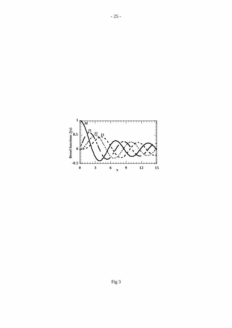
Where Ji are the Bessel functions of integer order i (Fig.2). If the vibration amplitude is sufficiently

low with respect to the characteristic length of the fringe contrast decrease, C(z)≈C(z0). Equation 9

shows that the interferometric signal is composed of : a continuous term, a component at the

excitation frequency and a number of non zero even and odd harmonics increasing with the

vibration amplitude [19] (Fig.2). A harmonic analysis of the signal is thus generally necessary for a

quantitative evaluation of the vibration amplitudes. For very low vibration amplitudes a such as

a<<λmc/4π, the Bessel functions can be approximated as follows : J0(4πa/λmc)≈1,

J1(4πa/λmc)≈2πa/λmc and Ji(4πa/λmc)≈0 for i>1. In that case a harmonic analysis is no longer

necessary because the interferometric signal is then only composed of a constant term, and a term at

the excitation frequency with an amplitude proportional to a :

)sin(4)4sin()()4cos()(1),,( 1000000 φωλ

πϕλ

πϕλ

π +∆+−∆++=

ta

mcz

mczCIz

mczCItyxI (10)

- 7 -

Equation 9 and 10 show that to maximize the sensitivity of the vibration amplitude measurements,

it is necessary to adjust and maintain the condition 2/)1k2(/z4 mc0 πϕ∆λπ +±=+ where k is an integer.

This is usually done by an active feedback stabilization circuit (see for example [25]). In our case it

is obtained by regularly adjusting the constant term (the signal after low pass filtering) at its mid

value when z0 is varied. The advantage is to be able to take into account the variation of the

background term with a when the vibration amplitude is not very low (see equation 9).

II.3 Stroboscopic measurements

For vibration modes profiling with a stroboscopic source, a light pulse of width δT, synchronized

with the vibration excitation source but with an adjustable delay time t0 is used to freeze the device

vibration at any time of the vibration cycle (Fig.3). The light detected by the camera is integrated

over a time T0 related to the video rate, which, for micromechanical devices, is always very large

with respect to the period T=2π/ω of the vibration. For a pixel of coordinates x,y the detected

intensity is then :

∫+

−

=2/

2/

0

0

),,(),(Tt

Tt

dttyxINyxIδ

δ

(11 )

where N is the integer part of (T0/T).

A simple calculation shows that :

))(cos(2/

)2/sin())(cos( 10

2/

2/1

0

0

φωωδ

ωδδφω

δ

δ

+=+∫+

−

tnTn

TnTNdttnN

Tt

Tt

(12)

Therefore the amplitude of each time-varying term with pulsation nω in Eq.9 is reduced by an

amount decreasing with δT /T and increasing with n.

In the general case, the expression of detected intensity is from equations 9,11 and 12 :

++= )

a4(J)z

4cos()z(C1ITK)t,y,x(I

mc

00

mc

0 λπ

ϕ∆λπ

δ

))t(k2cos()a4

(J2/Tk2

)2/Tk2sin()z

4cos()z(CITK2

10

mc

1k k20

mc

0φω

λπ

ωδωδ

ϕ∆λπ

δ +++ ∑∞

=

))t)(1k2sin(()a4

(J2/T)1k2(

)2/T)1k2sin(()z

4sin()z(CITK2

10

mc

0k 1k20

mc

0φω

λπ

ωδωδϕ∆

λπδ ++

+++− ∑

∞

= + (13 )

- 8 -

For low vibration amplitudes and short light pulses such as sin(nωδT/2)/nωδT/2≈1 for all harmonics

really present in the signal and by using Bessel function summation rules [24], we obtain an

expression of the detected intensity similar to the static case :

∆++++= ))sin(

44cos()(1),( 10000 ϕφω

λπ

λπδ tazzCITKyxI

mcmccquasistati (14)

The vibration modes can then be measured without distortion from the phase of the interferometric

signal. As micromechanical devices have often both high resonant frequencies and high quality

factors, the condition of short pulses (δT/T<<1) and low vibration amplitudes is not always satisfied

at resonance. The measured vibration modes are then distorted in a complex manner with a

maximum error occuring for points having the maximum vibration amplitude. The prediction of this

distortion is not straightforward, because the number of non zero terms in Equation 13 depends on

the vibration amplitude through the Bessel functions, and because the duty cycle δT/T affects both

the fringe contrast and the phase of the interferometric signal. This will be discussed in more detail

in a future paper from simulation results which are in progress.

II.4 Fringe pattern Fourier transform analysis

The equations of the interferometric signal I(x,y) for static (Eq.2) and stroboscopic (Eq.14)

measurements can both be written in the simple form :

)(cos)(B)(A)(I G/y,G/xG/y,G/xG/y,G/xy,x Φ+= (15)

The phase Φ contains the required information for static deformations profiling with continuous

illumination and for mode shapes profiling with stroboscopic illumination : ϕ∆λπΦ += 0mc

z4 for

static measurements while ϕ∆φωλπ

λπΦ +++= )tsin(a4z4 10

mc0

mc for stroboscopic measurements.

Note that by substracting the static phase from the stroboscopic phase, the initial deformation of the

microdevice, the height variations due to steps and the variations of ∆ϕ due to material changes

along the microdevice surface are automatically eliminated from the mode shape profile. For an

accurate measurement it is imperative to extract Φ independently from the variations of the

background intensity A and of the contrast B on the sample surface. Numerous temporal or spatial

methods have been proposed to realize this operation from a 2D digitized fringe pattern [26,27]:

phase stepping, spatial-carrier phase stepping, sinusoid fitting, frequency domain analysis,…or a

- 9 -

combination of them. In this paper, the Fast Fourier Transform (FFT) analysis has been chosen

because it is very robust and it requires only one interferogram [27-39]. Phase stepping methods

have potentially a better resolution, but they need several images (≥3) having the same background

and contrast maps. These conditions are difficult to obtain during vibrometry measurements and the

contrast is always z dependent when a high numerical aperture interferometric objective and/or a

light source with limited coherence are used. We applied FFT analysis to interferogram recorded on

tilted samples but Kreis et al. [38] showed that, by adding few processing steps, it can be extended

to non-tilted samples. For tilted samples with spatial frequency νx=ν0x along the x direction and

νy=ν0y along the y direction, I(x,y) becomes :

I(x,y) = A(x/G,y/G)+B(x/G,y/G) cos [2πι(ν0xx+ν0yy)+Φ] (16)

Following the classical approach (see for example [36]), it can first be rewritten as :

I(x,y) = A +B'expi2πτ(ν0xx+ν0yy)+B'* exp-i2πτ(ν0xx+ν0yy) (17)

Where B'=1/2 B(x,y) expiΦ and B'* is its complex conjugate.

Applying 2D Fourier transform to this equation, and using low case letters for FFT quantities, weobtain :

ι(νx, νy) = a(νx, νy)+b'(νx-ν0x, νy-ν0y)+b'*(νx+ν0x, νy+ν0y) (18)

This frequency spectrum is band-pass filtered around the carrier frequencies to isolate the lobe b' (or

b'*) which is then translated to the origin in the spatial frequency domain to remove the carrier.

Finally an inverse FFT is performed and the complex logarithm of the result B'(x,y) is calculated :

log|B'(x/G,y/G))|= Log|1/2B(x/G,y/G) |+iΦ(x/G,y/G) (19)

The imaginary part provides Φ(x/G,y/G) with good accuracy and without significant influence of

the background and contrast variations on the image [27-39]. If necessary, the contrast variation can

be calculated from the real part of equation 19 or more directly from the modulus of B'.

- 10 -

III. Experimental set-up

III.1 Optical system

The optical part of the vibrometer is schematised in Fig.4. It was designed as an extension of a

commercial white light fringe scanning optical profilometer [40]. Consequently, the whole system

has inherently the capabilities of 3D static profiles measurements of microdevices with (sub)micron

spatial resolution and nanometric vertical resolution. We demonstrated previously that the same

system can be configured for point measurements of vibration spectra with simultaneous

visualisation at video rate of time averaged vibration modes and for automatic bulge testing of

micromachined membranes [19]. The system is based on a standard reflection optical microscope

on which two light sources can be mounted simultaneously and selected with a commutable mirror.

According to the experiments, we use either a monochromatic sodium discharge lamp (λ=589 nm),

a stroboscopic quasi monochromatic source made with an 5x5 array of superluminescent amber

LED (Light Emitting Diodes) (λ=590 nm) or a low coherence tungsten-halogen white light source

(λmean ≈ 6600 nm). Most of the experiments here were performed with the LED array source whose

characteristics will be studied in part III.3. The illumination path (not shown in Fig.4) includes a

diffusing plate at the entrance and the usual lenses, field diaphragm,view diaphragm and reflector

found in classical optical microscopes. The microscope turret is equipped with Michelson X5 and

Mirau X40 interferometric objectives each one composed of an infinity corrected objective and a

miniaturized interferometer located below. Their main characteristics are given in table I.

Interference fringes result from the recombination of the light wave reflected on the internal

reference mirror and on the sample surface. Both interferometric objectives have a set of reference

mirrors with various reflectivities (5%, 25%,50%,85%) which can be selected and tilted in 2

perpendicular directions in order to optimize the fringe contrast, orientation and spacing. Static or

time-averaged interferograms can be visualized with the microscope oculars or acquired at video

rate by a 8 bits monochrome, 2/3 inches, 768x572 square pixels (11µm), CCD (Charged Coupled

Devices) camera connected to a frame grabber PC card. Vibration-induced fringe movement at any

point of the microdevice can also be detected through the XY translatable circular diaphragm D

(Fig.4) and the imaging lenses L1 and L2 by a fast (0.65ns) and sensitive (100µA/nW) miniature

photomultiplier. As discussed previously [19], the sensitivity and the spatial resolution of vibration

spectra point measurements with this detection system is mainly determined by the diaphragm

diameter, the magnification of the objective and the reduction factor of the C mount on which it is

mounted. With a 50µm in diameter diaphragm, a x40 Mirau objective, a 1x C mount and a 50 mW

Na light source, measurements of subnanometric vibration amplitudes of micromechanical devices

- 11 -

with a spatial resolution downto 1.25 µm and a frequency bandwidth >4MHz have been

demonstrated [19]. For all vibration measurements the sample substrate was glued with a silver

paste on a piezoelectric PbxZrTiO31-x (PZT) disk metallized with silver on both sides. The disk

itself is glued with conductive epoxy paste on a Cu covered glass flat plate and electrical

connections are bonded as indicated in Fig.4. The sample holder plate can be translated vertically

with a piezoelectric PZT translator via a parallelogram mechanism using flexible pivots. The PZT

translator has a vertical range of 15 µm and includes a stress gauge sensor for close loop control. It

is screwed on a tilting table mounted on the microscope table.

III.2 Driving and detection electronics

To perform a vibrometry measurement, the whole sample is excited in vibration by applying to the

piezoelectric disk a sinusoidal voltage coming from the first channel of a double channel, 15 MHz

bandwidth, waveform generator.

In the case of point vibration measurements with the photomultiplier, a lock-in detection technique

was used (Fig.5). The sinusoidal signal of the second channel was synchronized at the same

frequency or at an an integer multiple of it and used as a reference signal of a 10 MHz bandwidth

double lock-in amplifier. The signal input of the lock-in amplifier is fed with the amplified and high

pass filtered (1kHz) output of the photomultiplier (PM). The aim of this high pass filtering is to

reject the 100Hz modulation of the Na lamp light power and its harmonics. This is not necessary for

the other light sources. This detection electronics allows measurements of vibration spectra without

the need of a phase adjustement at each frequency between the PM signal input and reference input

of the lock-in amplifier and provides the capability of a harmonic analysis of the PM signal. As

mentioned in part II.2 such a harmonic analysis is necessary for quantitative measurements of

vibration amplitudes larger than λ/4π . The PM output is also low pass filtered (10 Hz) and this

signal is used to maintain the mean optical path difference of the interferometer at the middle of a

fringe (see Eq.10 and discussion below). This is necessary for large frequency scans during which

the vertical mechanical drift of the sample holder is no longer negligible. Instead of using a

feedback circuit, the stabilisation was performed by software to prevent the generation of an

unwanted additional oscillation of the sample: the frequency scan is periodically interrupted and the

sample is moved vertically with the PZT translator around its current position by a amount z

comprised between λ/2 et λ to find the mid fringe position.

- 12 -

During stroboscopic measurements, the waveform generator second channel is used to drive the

LED source (Fig.6) with a square signal having a duty cycle in the range 3% to 20%. The mean

LED peak current was adjusted to 100 mA giving an upper limit of 20 mA average current for a

20% duty cycle. For the measurement of the vibration modes at any time of the vibration cycle, the

two waveform generator channels are synchronized at the same frequency and their phase

difference is adjusted. For real-time observation of the vibration modes at reduced speed, the two

channels are driven at slightly different frequency (∆f<1Hz) which generates a linear phase ramp.

III.3 Stroboscopic LED source characteristics

The LED source tested and used for all experiments described in this paper is a 5x5 array of

superluminescent LED ( λ=590 nm) each with a typical luminous intensity of 9600 mCd for a

current of 20 mA and a divergence angle of 6°. It was mounted directly on the microscope without

any optics. The total light power reaching the sample surface was 11µW for the x5 Michelson

objective and 1.5µW for the x40 Mirau objective for a current of 20 mA. Owing to the diffusing

plate at the entrance of the illumination path no light structuring was observed and the light

homogeneity at the sample level was about 20%.

The contrast of the interferometric signal was measured for the LED source and for the two

interferometric objectives by recording with the camera the intensity during a vertical scan of a

Al/Si flat sample. In both cases a 85% reflectivity reference mirror was used. The measurements

were averaged over a 3x3 pixels region located at the image center. The result obtained for the

Michelson x5 objective (NA=0.12) is shown in Fig. 7. The contrast envelope determined by a

Fourier analysis of the signal could not be fitted with satisfactory parameters by a gaussian curve.

For this objective, the contrast is limited by the source coherence length as its depth of field is large

(Table I). The characteristic lengths Lc1/2 and Lc1/e for which the contrast is divided by 2 and 1/e are

respectively 3.65 µm and 4.7 µm. Fig.6 shows that more than 50 fringes (15 µm) can be detected

which is largely sufficient for the measurement of most micromechanical devices. No enlargement

of the fringe spacing could be evidenced for this objective around the maximum of the contrast

envelope (λmc=0.590 nm). This is consistent with the theoretical value of the correcting factor

f=0.3% [23]. However an increase of fringe spacing was found beyond about 3.5 µm from the

maximum of the contrast envelope. For the x40 Mirau objective (NA=0.6), the fringe contrast

envelope is much narrower and is clearly limited by the objective depth of field (Fig.8). The values

of Lc1/2 and Lc1/e extracted from the contrast envelope are 0.9 µm and 1.25 µm and the number of

usable fringes is only about 10 (3 µm ). As expected these values are increased when the field

- 13 -

diaphragm aperture of the microscope illumination path is reduced. At the same time, the

oscillations of the contrast envelope (Fig.8) disappear. This shows that they are not due to a

misalignment of the interferometer [41]. A rapid evaluation shows that the fringe spacing

enlargement is about 9.1%, a value lower than the value (about 13%) expected from theoretical

calculations [23].

The resonant frequencies of micromechanical devices reach often several hundred kHz or more. For

stroboscopic measurement at such frequencies short light pulses must be used. The intrinsic

response time of the LEDs used is 17 ns. In our case the effective rise time of the light pulse is

mainly limited by the driving electronics and is ≤50 ns. For a 5% duty cycle this corresponds to a

theoretical maximum measurement frequency of 1MHz.

IV Experimental results

IV.1 Micromechanical devices fabrication

Evaporated Aluminium cantilever microbeams and rf sputtered chromium rectangular membranes

were fabricated as test samples for the stroboscopic measurements of the vibration modes. The

aluminium cantilever microbeams were fabricated by surface micromachining with the process

described in ref [42]. Briefly it consists in patterning the Al film and releasing the microbeams by a

selective and isotropic SF6 plasma etching of the silicon substrate in a barrel type reactor. A low rf

power was used during plasma etching to avoid the generation of thermally induced stress gradients

[42]. The Cr membranes were fabricated by conventional KOH bulk micromachining of the silicon

substrate from the rear side. A teflon substrate holder with O-rings was used to protect the film

during etching. Cr film compressive stress was minimized by performing the deposition at a high

pressure to reduce the peening effect as we have done previously for sputtered tungsten

membrane[43]. Nevertheless, as shown below, the Cr residual film stress was still sufficiently

compressive to induce a slight buckling of the membrane.

IV.2 FFT interferogram analysis

The flow chart giving the steps we used to implement a fully automated FFT processing of the

interferograms is shown in Fig.9. The main steps are indicated in solid boxes. Additional steps used

for a faster processing but with a reduced spatial resolution are indicated in boxes with dashed lines.

They are used for quasi real time visualization of the 3D profiles of the vibration modes. Boxes with

dotted lines correspond to the case of differential profiles calculation. This FFT interferogram

- 14 -

processing (Fig.9) includes various refinements described below. Starting from the acquired image

(step 1), a region of interest is defined with a mask and extended in x and y direction to the nearest

power of 4 by zero padding (step 2) in order to use afterwards efficient 4n FFT algorithms (step 3),

to limit windowing effects and to make room for fringe extrapolation (step 5). The next step is the

automatic search of the carrier frequencies by peak detection (step 4). It is performed only once on a

reference static image before vibration measurements. For the following measurements, the same

values of the carrier frequencies are used (step 4´) and this step is skipped. For this step, a mask is

used to make the peak detector insensitive to the contrast modulation (around zero frequency) and

to parasitic carriers. Then the fringes are extrapolated up to the image boundaries on areas outside

the micro-device and on areas masked by dust particles on the optics or on the sample (step 5). We

used the efficient algorithm proposed by Roddier et al. [32]. It uses the iterative sequence shown in

the solid boxes at the right side of Fig.9. Briefly, it consists in extracting, in the frequency domain

by a narrow filtering, the data corresponding to the carrier frequencies while keeping some

information of the fringe modulation due to the device deformation. Then the corresponding fringes

are extended in the space domain by an inverse FFT in all areas except in the microdevice area

where the original data are kept intact. This procedure is repeated with a variable filter size until the

contrast of the extrapolated fringes is satisfactory. The next step of the main processing block (step

6), is a 2D band pass filtering of the lobe around the carrier by using a circular mask with apodized

borders. After translation to the origin (step 8), the inverse FFT of the image is computed (step 9)

and the phase image is calculated from the imaginary part of its logarithm (step 10). The phase

obtained is a wrapped phase modulo 2π. For vibration modes profiling, this wrapped phase of the

static interferogram is substracted (step 10´) so phase discontinuities related to the device surface

steps or reflection phase shifts steps are removed before the unwrapping process (step 11). In

addition, noise is removed owing to the efficient filtering capabilities of the FFT analysis and the

fringe extrapolation step remove the fringes discontinuities at the device boundaries and around

areas masked by dust particles. Consequently, for the micro-devices investigated (micro-cantilever

beams and micromachined membranes), it was not necessary to use the numerous advanced

unwrapping algorithms proposed previously [44]. A simple and fast unwrapping beginning from the

image center along the corresponding column then along the lines starting from it was sufficient.

Finally, a 3D surface plot of the vibration mode is drawn from the data of the unwrapped phase.

For fast visualization of the vibration modes, a full spatial resolution is not necessary. So after

acquisition, the interferogram is resampled to reduce its size by a factor 3 (step 1’). This is valid

- 15 -

only if there are more than 6 pixels per fringe what is usually the case. Before the 3D profile

display, the interferogram is again resampled for accelerating its calculation.

Fig.10 and 11 illustrate this FFT analysis in the case of the measurement of the static and dynamic

displacements of a 100 µm long, 10 µm wide, 0.6 µm thick aluminum cantilever microbeam. The

three images shown in Fig.10 correspond to a static measurement. The corresponding images during

dynamic measurement are very similar because the vibration amplitudes are only a very small

fraction of the fringe spacing. The first image (Fig.10a) shows the interferogram recorded on the

tilted sample at full spatial resolution by using the Mirau X40 interferometric objective with a 85%

reflectivity reference mirror and the CCD camera. Only a part of the image around the microbeam

is shown. There is a clear variation of the fringes contrast in the interferogram. As discussed in part

III.3, it is mainly due to the limited depth of field of the objective. The result of fringes

extrapolation with 32 iterations is displayed in Fig.10b. In this particular case, a large number of

iterations is necessary because the area covered by the microdevice is only about 5% of the full

image. The fringe contrast ouside the device area could be increased by using more iterations but it

is not necessary for the subsequent processing. Note that in this particular case, the fringes

extrapolation produces a fringe split at the bottom right of the microbeam (indicated by a black

arrow). This leads to a defect in the unwrapped phase at the end of the processing but as the

unwrapping is started from the center of the image, it does not affect phase data corresponding to

the microdevice. The 2D Fourier spectrum in logarithm scale (Fig.10c) shows that with a sufficient

tilt, the carrier and and its modulation lobe are sufficiently separated from the background and the

fringe contrast modulation contributions (center of the spectrum and lines starting from it) to allow

a fully automated detection of the carrier frequencies and a band pass filtering of the modulation

lobe with a predetermined window size. The filter window used is indicated by a black circle. The

next images (Fig.11) show the wrapped phase (Fig.11 a) and the unwrapped phase (Fig.11 b) for the

static deflection measurement. At last, the unwrapped phase image of the second vibration mode

(f=296.1kHz) after correction of the static displacement is shown in Fig.11c. As expected the

vibration mode has a node close to the center of the beam.

IV.3 Dynamic characterization of Al microbeams

The measured vibration spectrum of the same Al cantilever microbeam as above is plotted in

Fig.12. This spectrum was measured by lock-in detection at the end of the cantilever beam with a

spatial resolution of 2.5 µm (100µm in diameter diaphragm). Three main resonances at 48 kHz,

- 16 -

296.1 kHz and 816 KHz corresponding to the 3 first flexural modes can easily be distinguished.

Values of the film Young’s modulus computed [45] from these 3 resonant frequencies are

respectively 69 GPa, 67 GPa and 65 GPa while the young’s modulus of bulk aluminum is in the 69-

72 GPa range. No clear explanation of the decrease of the measured Young’s modulus with mode

order could be found as measurements on similar Cr microbeams fabricated by the same process did

not show such a behaviour.

Stroboscopic measurements with FFT interferogram analysis of the vibration modes were

performed at these three frequencies with a light pulse duty cycle of 5 %. Fig.13 gives a comparison

of the computed and measured profiles of the vibration modes. The static profile of the microbeam

is also plotted with a reduced scale (1/3) on the same figure. The measured mode shapes were

obtained by profiling the unwrapped phase along the microbeam length after correction of the static

profile. The theoretical mode shapes were computed from reference [45] and were vertically scaled

by a constant factor to fit the experimental ones. Fig.13 shows that there is a close agreement

between the measured and theoretical ones. The slight discrepancies observed likely arise from the

distortion effect related to the excessive light pulse width used for the vibration amplitudes

measured (see part II.3) but the underetching at the clamped end inherent to the fabrication process

[42] may also contribute to the differences. To give an idea of the distorsion effect, an increase ot

the duty cycle from 3% to 20% gave a 10% increase of the measured vibration amplitude for a

vibration amplitude of 257nm.

IV.4 Dynamic characterization of Cr membranes

A chromium rectangular membrane with approximative dimensions 600 µm x 1200 µm x 1µm was

used as a first test sample. For this sample, all measurements were performed with the Michelson x5

interferometric objective with a 85% reflectivity mirror. Its static 3D deformation profile

determined by FFT analysis of an interferogram recorded after sample tilting is shown in Fig.14. It

is slightly buckled with an unexpected deformed shape as it is almost flat along the membrane

borders. Nevertheless it was judged still suitable for the evaluation of the optical system. A

vibration spectrum of this membrane was measured near a corner by lock-in detection with a spatial

resolution of 20 µm (Fig.15). The vibration spectrum contain many resonant peaks difficult to

identify without a visualisation or a profiling of the vibration modes shapes. This is a typical

situation for micromachined membranes which have complex vibration modes with low quality

factors due to air damping. Stroboscopic measurements of the vibration modes were performed with

a light pulse duty cycle of 5% for the resonant peaks indicated by letters in Fig.15. As mentioned

- 17 -

previously in part IV.2, the FFT interferogram analysis can be largely accelerated by using

resampled interferograms. In addition, for membranes, the fringe extrapolation can be reduced to a

few iterations only. With a 500 MHz PC, by reducing the original interferogram size to 256x256

pixels, the total processing time is about 150 ms once a reference static profile with the same tilt is

measured. This processing time includes the substraction of the initial static 3D profile and the 3D

plot visualisation. Such a reduced processing time allows a quasi real-time measurement of the

vibration modes 3D profiles. This quasi-real time operation mode can as well be used for

microbeams but the processing time is about 3 times longer because fringe extrapolation is more

critical. Examples of quasi real-time 3D profiles for some characteristic vibration modes of the Cr

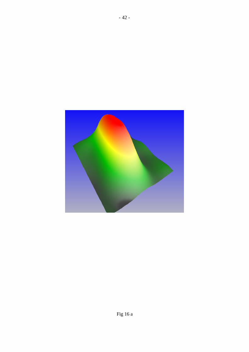
membrane are shown in Fig.16 and 17 together with the calculated modes shapes [9,46]. The first

mode shown (Fig.16a) at 126.9 kHz is symmetrical and corresponds to the theoretical first natural

mode of a perfect membrane (Fig.16b). The next vibration mode 3D profiles are antisymmetrical

with a central nodal line (Fig.17). As a last example, a complex 5x2 vibration mode measured at

496.8 kHz is shown in Fig.18.

All these vibration modes were measured with a phase lag between the PZT disk driving voltage

and the LED array driving voltage adjusted to give the maximum amplitude. Actually the vibration

mode profiles can be measured at any time of the vibration cycle. This is illustrated in Fig.19 which

shows a 3x1 vibration mode with different delays between the excitation and the light pulse. Such a

measurement is useful to check if the oscillation is purely vertical and symmetrical around the static

position without wave propagation. Then the vibration mode is purely harmonic without coupling

with other vibration modes. For the example of Fig.19, the mode has a relatively good symmetry

despite the initial buckling of the membrane.

As indicated in the figure captions, the maximum vibration amplitudes for the different modes

shown are in the range 14-130 nm. This demonstrate the high sensitivity of the stroboscopic

measurements. The measurement performances depends on many factors which are under

investigation. A preliminary evaluation showed that systematic errors limit the minimum vibration

amplitude which can be measured to about 3-5 nm and that beyond this value the measurement

resolution is below 1nm

V Conclusion

Microscopic interferometry is used for a long time for static 3D surface profiling with high lateral

and vertical resolution. By using a LED stroboscopic light source and an automatic fringe pattern

- 18 -

analysis, we have demonstrated that its 3D profiling capabilities can be extended to the

measurement of vibration modes of micromechanical devices up to at least 800 kHz.. In addition,

owing to a phase demodulation of the interferograms by Fast Fourier Transform, a quasi real time

visualisation of the vibration mode 3D profiles can be achieved. This full field measurement can be

combined with point measurements of the vibration spectra to obtain a complete analysis of out-of-

plane vibrations of MEMS. The main limitation of the system is a slight distortion of the vibration

mode shapes for large vibration amplitudes. Work is in progress to quantify and correct this

distortion.

Acknowledgments

This work was supported by funds from the french National Center of Scientific Research (CNRS)

through the Microsystems program, from Paris south university and from Institut d´Electronique

Fondamentale. The authors wish to thank Philippe Nerin from Fogale Nanotech company (Nimes,

France) for stimulating discussions.

References

1. Petersen P E, Guarnieri C R. Young’s modulus measurements of thin films using micromechanics. J.Appl.Phys.1979;50(11): 6761-6766

2. Hoummady M, Farnault E, Kawakatsu H, Masuzawa T. Applications of Dynamic Techniques for accuratedetermination of Silicon Nitride Young’s Moduli. Proc. Transducers 1997: 615-618

3. Ye X Y, Zhou Z Y, Yang Y, Zhang J H, Yao J. Determination of the mechanical properties of microstructures.Sensors and Actuators 1996; A 54: 750-754

4. Tabib-Azar M, Wong K, Ko W. Aging phenomena in heavily doped (p+) micromachined silicon cantilever beams.Sensors and Actuators 1992; A 33: 199-206

5. Zhang L M, Uttamchandi D, Culshaw B. Measurement of the mechanical properties of silicon microresonators.Sensors and Actuators 1991; A29:79-84

6. Bouwstra S, Geijelaers B. On the resonant frequencies of microbridges. Proc. Transducers 1991:538-542

7. Nicu L, Temple-Boyer P, Bergaud C, Scheid E, Martinez A. Experimental and theoretical investigations on nonlinear resonances of composite buckled microbridges. J Appl Phys 1999; 86:5835-5840

8. Manceau J F, Robert L, Bastien O, Oytana C, Biwersi S. Measurement of residual stresses in a plate using avibrational technique-application to electrolytic nickel coatings. J. Microelectromechanical Systems 1996;5(4):243-249.

9. Jonsmann J, Brouwstra S. On the resonant frequencies of membranes. Proc. Micromechanics Europe 1995 :225-229

10. Sader J E. Frequency response of cantilever beams immersed in viscous fluids with applications to the atomic forcemicroscope. J Appl Phys 1998; 84(1): 64-76

11. Andres M V, Tudor M J, Foulds K W H. Analysis of an interferometric optical fiber detection technique applied tosilicon vibrating sensors. Electron Lett 1987;23(15) :774-775

- 19 -

12. Guttierez A, Edmans D, Seidler G, Conerty M, Aceto S, Westervelt E, Burrage M, Cormeau C. MEMS metrologystation based on two interferometers. Proc SPIE 1997; 3225:23-31

13. Turner K L, Hartwell P G, MacDonald N C. Multidimensional MEMS motion characterization using laservibrometry. Proc. Transducer 1999: 1144-1147

14. Cloud G. Optical methods in engineering analysis. Cambridge University Press 1995

15 Brown G C, Pryputniewicz R J. Holographic microscope for measuring displacements of vibrating microbeamsusing time-averaged, electro-optic holography.Opt Eng 1988; 37(5): 1398-1405

16. Aswendt P, Höfling R, Hiller K. Testing microcomponent by speckle interferometry. Proc. SPIE 1999; 3825:165-173

17. Osten W, Jüptner W, Seebacher S, Baumach T. The qualification of optical measurement techniques for theinvestigation of materials parameters of microcomponents. Proc. SPIE 1999; 3825:152-164

18. Burdess J S, Harris A J, Wood D, Pitcher R J, Glennie D J. A system for the dynamic characterization ofmicrostructures. Microelectromechanical Systems 1997;6(4):322-328

19. Bosseboeuf A, Gilles J-P, Danaie K, Yahiaoui R, Dupeux M, Puissant J-P, Chabrier A, Fort F, Coste P, A versatilemicroscopic profilometer-vibrometer for static and dynamic characterization of micromechanical devices. Proc. SPIE1999; 3825: 123-133

20. Hart M, Conant R A, Lau K Y, Muller R S. Time resolved measurement of optical MEMS using stroboscopicinterferometry. Proc. Transducers 1999, 470-473

21. Nakano K, Hane K, Okuma S, Eguchi T. Visualization of 50 MHz surface acoustic wave propagation usingstroboscopic phase-shift interferometry. Optical-Review 1997;4(2):265-269

22. Born M, Wolf E, Chap.X: Interference and diffraction with partially coherent light. In: Born M, Wolf E editors,Principles of Optics, Cambridge University Press, 7th edition, 1999

23. Sheppard C J., Larkin K G. Effect of numerical aperture on interference fringe spacing. Appl Opt1995;34(22):4731-4734

24. Olver F W J. Bessel function of integer order. In : Abramovitz M and Stegun I A editors, Hand book ofmathematical functions, 9th edition, Dover Publications, N.Y. 1971

25. White R G, Emmony D C. Active feedback stabilisation of a Michelson interferometer using a flexural element. JPhys E: Sci Instrum 1985;18 :658-663

26.Creath K, Temporal phase measurement methods. In: Robinson D W, Reid G T, editors. Interferogram analysis;digital fringe measurement techniques. Institute of Physics Publishing, 1993

27. Kujawinska M, Spatial phase measurement methods: In: Robinson D W, Reid G T, editors. Interferogram analysis;digital fringe measurement techniques. Institute of Physics Publishing, 1993

28. Takeda M, Ina H, Kobayashi S. Fourier-transform method of fringe pattern analysis for computer-based topographyand interferometry. J Opt Soc Am 1982; 72(1) : 156-160

29. Takeda M, Mutoh K. Fourier transform profilometry for the automatic measurement of 3-D object shapes. Appl Opt1983; 22 (24) : 3977-3982

30. Bone D J, Bachor H-A, Sandeman R J. Fringe-pattern analysis using a 2-D Fourier transform. Appl Opt 1986;25(10):1653-1660

31. Macy W W. Two-dimensional fringe-pattern analysis. Appl Opt 1983; 22 (23): 3698-3901

- 20 -

32. Roddier C, Roddier F. Interferogram analysis using Fourier transform techniques. App Opt 1987; 26(9) : 1668-1673

33. Gu J, Chen F. Fourier-transformation, phase iteration and least-square-fit image processing for young's fringepattern. App Opt 1996; 35(2) 232-239

34. Gorecki C. Interferogram analysis using a fourier transform method for automatic 3D surface measurement. PureAppl Opt 1992 : 103-110

35. Kostianovski S, Lipson S G, Ribak E N. Interference microscopy and Fourier fringe analysis applied to measuringthe spatial refractive-index distribution. Appl Opt 1993; 32(25) : 4744-4750

36. Nugent K A. Interferogram analysis using an accurate fully automatic algorithm. Appl Opt 1985; 24(18) : 3101-3105

37. Talamonti J J, kay R B, Krebs D J. Numerical model estimating the capabilities and limitations of the fast Fouriertransform technique in absolute interferometry. Appl Opt 1996; 35(13) : 2182-2191

38. Kreis T. Digital holographic interference phase measurement using the Fourier transform method. J.Opt.Soc. Am.1986; A3:847-855

39. Pandit S M, Jordache N. Data-dependent-systems and Fourier-transform methods for single-interferogram analysis.Appl Opt 1995; 34(26) : 5945-5951

40. Microsurf 3D. Fogale Nanotech, Nimes, France. http://www.fogale.fr

41. Ning Y N Ning, Grattan K T V, Palmer A W. Fringe beating effects induced by misalignment in a white-lightinterferometer. Meas Sci Technol 1996;7:700-705

42. Boutry M, Bosseboeuf A, Coffignal G. Characterization of stress in metallic films on silicon with micromechanicaldevices. Proc. SPIE 1996;2879:126-134

43. Bosseboeuf A, Dupeux M, Boutry M, Bourouina T, Bouchier D, Debarre D. Characterization of W films on Si andSiO2/Si substrates by X-ray diffraction, AFM and blister test adhesion measurements. Microsc Microanal Microstruc1997 ;8 :261-272

44. Ghiglia C, Pritt M D. Two-dimensional unwrapping. Wiley &sons, 1998

45. Rao S S. Mechanical vibrations, Addison Wesley Publishing, 3rd edition, 1995

46. Leissa A W. Vibration of plates, Acoustical Society of America Publishing 1983

- 21 -

Figure captions

Fig 1 Simplified scheme of the experimental set-up

Fig.2 Bessel functions of integer order J0, J1, J2, J3 as function of the normalized vibration amplitudex= 4πa/λmc.

Fig 3 Timing of stroboscopic measurements

Fig 4 Configuration of the optical system.

Fig 5 Driving and lock-in detection electronics for point vibration measurements

Fig.6 Driving and detection electronics for stroboscopic vibration measurements

Fig 7 Interferometric signal as function of sample vertical position for the LED array source and theMichelson x5 objective

Fig 8 Interferometric signal as function of sample vertical position for the LED array source and theMirau x40 objective

Fig 9 FFT interferogram analysis flow chart

Fig.10 FFT analysis of an interferogram recorded on a 100µmx8µmx0.6µm Al cantilevermicrobeam.a) Initial static interferogram. b) Partial view after fringe extrapolation.c) FFTspectrum.

Fig.11 FFT analysis of an interferogram recorded on a 100µmx8µmx0.6µm Al cantilevermicrobeam.a) Wrapped and b) unwrapped static deflection phase; maximum static deflexion -0.63µm. c) 2nd flexural mode (f=296.1 kHz) after static deflection substraction; maximum vibrationamplitude 180nm.

Fig 12 : Vibration spectrum of an Al cantilever microbeam: a) around the first flexural resonance b)around the second flexural resonance c) around the third flexural resonance. The PZT disk drivingvoltage is 1Vpp for the 1st and the 2nd mode and 10Vpp for the 3rd mode.

Fig 13 Computed and measured vibration mode profiles for the 3 first flexural resonances of an Alcantilever microbeam at 48 kHz, 296.1 kHz and 816 kHz respectively. The profile of the initialstatic deflection is included for comparison at 1/3 scale.

Fig 14 Static 3D profile of a chromium rectangular membrane. The black solid line shows themembrane borders. Membrane dimensions: 1200µmx600µmx1µm ; maximum deflection 125nm.

Fig 15 Vibration spectrum of the Cr membrane. PZT disk driving voltage : 0.4 Vpp.Letters a to d show the modes measured by stroboscopic interferomety.

- 22 -

Fig 16 3D profiles of the first main vibration mode of the Cr membrane. a) Measured mode at f=126.9kHz; maximum vertical deflexion : 14nm.b) Normalized theoretical mode.

Fig 17 3D profiles of a 2x1 vibration mode of the Cr membrane. a) Measured mode shape at f=167.3 kHz; maximum vertical deflexion : 120 nm.b) Normalized theoretical mode shape.

Fig 18 3D profiles of a 5x2 vibration mode of the Cr membrane. f= 496.8kHz; maximum deflexion130 nm.

Fig 19 3D profiles of a 3x1 vibration mode of the Cr membrane with 0°,60°,120°,180° phase delaybetween the excitation at f=226.5kHz and the light pulses.

- 23 -

Fig.1

CCD

Tube Lens

Objective

Beamsplitter

ReferenceMirror

Sample

P(x,y)

P'

E'0

r1 E1

E1

E2 r2 E2

x/G

y/G

z

P''Monochromaticlight source E0

- 24 -

-3.00-2.00-1.000.001.002.003.004.00

Time

T0>>T

0

T

t0

Lig

htpu

lse

Exc

itatio

nsi

gnal

t0+T t

0+2T t

0+nT

δδT

Fig.2

- 25 -

Fig 3

-0.5

0

0.5

1

0 3 6 9 12 15

Bes

sel f

unct

ions

Ji(x

)

J0

J1J2 J3

x

- 26 -

Fig.4

PZT Voltageinput

Tube Lens

Objective

BeamSplitter

ReferenceMirror

Sample

CCDcamera

Glass platePZT disk

Microscope XYZ stage

θθstage

Piezoelectrictranslator Stress

sensor output

PM

f f2f

D L L

Parallelogrammechanism

- 27 -

Fig.5

PC

PZT disk

Na sourcePZT

translatorController

Photomultiplier

WaveformGenerator

1

Interferometer

IEEE

IEEE bus

PZT translatorI-V

converter

DoubleLock-inamplifier

in outref

<10Hz

>1kHz

0-100V

mirror

sensor

2

- 28 -

Fig 6

PC

PZT disk

+VLED array

PZTtranslatorController

CCDCamera

WaveformGenerator

1

2

Interferometer

IEEE

IEEE bus

PZT translator

0-100VSensor

Mirror

- 29 -

Fig.7

0

50

100

150

200

250

0 5 10 15

Lig

ht in

tens

ity

(A

.U)

Sample vertical position (µm)

- 30 -

Fig.8

0

50

100

150

200

0 5 10 15

Lig

ht in

tens

ity

(A

.U)

Sample vertical position (µm)

- 31 -

Fig.9

8 Fourier spacetranslation to the origin

5 Fringes extrapolation

1’

4’

1 Acquisition768x576 Greyscale image

2 Zero padding

3 2D FFT

9 Inverse 2D FFT

10 Phase extraction

11 Phase unwrapping

12 Final 3D profil

6 2D band-pass filteringaround carrier frequencies

10’

Reference wrappedphase substraction

2D band-pass filteringaround carrier frequencies

2D FFT

Inverse 2D FFT

Replace unmasked data byoriginal data

4 Peak detectionof the carrier

Resampling256x192 Greyscale image

7 Fourier spectrumcropping

Use referencecarrier

frequencies

- 32 -

Fig 10 a

- 33 -

Fig 10b

- 34 -

Fig 10c

- 35 -

Fig.11 a b c

- 36 -

Fig 12 a

0

0.05

0.1

0.15

0.2

40 45 50 55 60

Loc

k-in

Am

plifi

er o

utpu

t (V

)

Frequency (kHz)

- 37 -

Figure 12 b

0

0.05

0.1

0.15

0.2

0.25

0.3

290 295 300 305

Loc

k-in

Am

plif

ier

outp

ut (

V)

Frequency (kHz)

- 38 -

Figure 12 c

0

0.01

0.02

0.03

0.04

0.05

0.06

800 804 808 812 816 820 824 828 832

Loc

k-in

Am

plif

ier

outp

ut (

V)

Frequency (kHz)

- 39 -

-0 .4

-0 .3

-0 .2

-0 .1

0

0.1

0.2

0.3

-40 -20 0 2 0 4 0 6 0 8 0 100

1st Mode2 n d M o d e3rd ModeTheoryV

erti

cal

def

lex

ion

(µ

m)

D i s tance from c lamped end (µm)

Static x1/3

Fig 13

- 40 -

Fig 14

- 41 -

Fig 15

0

0.5

1

1.5

2

2.5

100 150 200 250 300 350 400 450 500

Loc

k-in

Am

plif

ier

outp

ut (

V)

Frequency (kHz)

(a) (b)

(c)

(d)

- 42 -

Fig 16 a

- 43 -

Fig 16 b

- 44 -

Fig 17 a

- 45 -

Fig 17 b

- 46 -

Fig 18 a

- 47 -

Figure 18 b

- 48 -

ϕϕ =ϕϕ0 ϕϕ=ϕϕ0+60° ϕϕ=ϕϕ0+120° ϕϕ=ϕϕ0+180°

Fig 19

- 49 -

Objective Numericalaperture

NA

ResolutionRo b

(µm)

Depth of fieldD

(µm)

CameraResolution Rc c

(µm)

Maximum tiltSlope andAngle

TS, ,TM d

µm/µm, (°)Michelson x5 0.12 4.03 ± 33,3 2.2 ± 0.134 , ± 3.8

Mirau X40 0.6a 0.59 b ± 1.08 b 0.275 ± 0.536, ± 28a Central obscuration not taken into account. b R0=0.82λ/NA for coherent light illumination [ ]. c Rc=pixelsize/magnification= (11µm/G). d TS=λ/4Rc and TM=tan-1(ΤS) for 2 pixels/fringe.

Tab.1 Interferometric objective characteristics for λ=0.59 nm