МИНИСТЕРСТВО ОБРАЗОВАНИЯ РЕСПУБЛИКИ БЕЛАРУСЬ

УЧРЕЖДЕНИЕ ОБРАЗОВАНИЯ «БРЕСТСКИЙ ГОСУДАРСТВЕННЫЙ ТЕХНИЧЕСКИЙ УНИВЕРСИТЕТ»

КАФЕДРА ВЫСШЕЙ МАТЕМАТИКИ

PROBABILITY THEORY

ELEMENTS OF MATHEMATICAL STATISTICS

учебно-методическая разработка на английском языке

Брест 2014

УДК 519.2(076)=111

Настоящая методическая разработка предназначена для иностранных студентов тех-нических специальностей. Данная разработка содержит необходимый материал по раз-делам «Теория вероятностей» и «Математическая статистика». Изложение теоретиче-ского материала по всем темам сопровождается рассмотрением большого количества примеров и задач, некоторые понятия и примеры проиллюстрированы.

Составители: Гладкий И.И., доцент Дворниченко А.В., старший преподаватель Каримова Т.И., к.ф.-м.н., доцент Лебедь С.Ф., к.ф.-м.н., доцент Шишко Т.В., преподаватель

Рецензент: Матысик О.В., заведующий кафедрой прикладной математики и техноло-гий программирования учреждения образования «Брестский государ-ственный университет им. А.С. Пушкина», к.ф.-м.н., доцент.

Учреждение образования «Брестский государственный технический университет», 2014

3

1. EVENT AND PROBABILITY

1.1 TRIAL AND EVENT

The probability theory is the science of rules of mass random phenomena. One can say that it’s the learning dealing with regularities of mass random phenomena. Known sources of the probability theory are: a)investigations of demographic processes [of population laws]; b) games of chance [games of luck, hazards].

A trial and an event are the main notions of the probability theory. Def. 1. A trial is a realization of some complex of conditions. It’s supposed that a trial can be arbitrary realized many times. Def. 2. An event is every fact, which can occur [appear, happen] or not occur in a trial.

Ex. 1 (see the table). Trial Events

1. Coin flip [coin tossing] “head” (occurrence of a head), “tail” 2. Dice toss(ing), fair dice rolling “1”, “2”, “3”, “4”, “5”, “6” 3. Drawing a ball from an urn containing a white and b black balls “white ball”, “black ball”

Events are usually denoted by capitals ( , , ,A B C …). There are impossible, certain and ran-dom events.

Def. 3. An event is called impossible if it can’t occur in any trial. Ex. 2. Occurrence of a head and a tail in one coin tossing. Def. 4. An event is called certain if it necessarily occurs in any trial. Ex. 3. Occurrence of a head or a tail in one coin tossing. Occurrence of at least one of the

digits 1, 2, 3, 4, 5, 6 in one dice rolling. Def. 5. An event is called random if it can occur or not occur in a trial. Ex. 4. All events fixed in Ex. 1. There are joint or disjoint events. Def. 6. Events ,A B are called joint [compatible] if they can occur together [or simultane-

ously] in a trial. Ex. 5. “head”, “head”; “tail”, “tail”; “head”, “tail”; “tail”, “head” if a trial implies double coin tossing. Def. 7. Events ,A B are called disjoint [incompatible, non-compatible] if they can’t occur to-

gether [or simultaneously] in a trial. Ex. 6. “head”, “tail” in one coin toss. Ex. 7. The events “1”, “2”, “3”, “4”, “5”, “6” are pairwise disjoint in one dice rolling. There are dependent and independent events. See the corresponding definitions below. Def. 8. One says that events , ...,A B C form a total [complete] group (of events) [ , ...,A B C

are only possible events, , ...,A B C are exhaustive events] if at least one of them occurs in any trial.

Ex. 8. Events “head” and “tail” in one coin toss. All the events “1”, “2”, “3”, “4”, “5”, “6” in one dice rolling.

Def. 9. Two events A and A (non A) are called opposite if they are disjoint and form a to-tal group.

Ex. 9. If A is “head”, then A (non A ) is “tail” (in one coin toss). If A is “1”,then A (non A ) is the occurrence of at least one of events “2”, “3”, “4”, “5”, “6”, A = {“2” or “3”, or “4”, or “5”, or “6”} (in one fair dice rolling).

4

1.2. ELEMENTS OF COMBINATORICS

Theorem 1 (fundamental principle of combinatorics). Let an action 1A be able to be done by 1n ways, an action 2A by 2n ways,…, an action kA by kn ways, then all these ac-tions can be done together [or simultaneously] by 1 2 3 kn n n n ways.

We’ll illustrate the validity of this statement with the help of the next example. Ex. 10. Let's suppose that one has a coins and b dice. Then he can take a coin and a die by

a ∙ b ways. ■Indeed, each coin generates 1 ∙ b = b pairs “coin-die”. Therefore, a coins generate a ∙ b pairs.■

Ex. 11. One has 2 coins, 3 ties and 5 books. He can take one coin, one tie and one book by 2 ∙ 3 ∙ 5 = 30 ways.

Main notions of combinatorics Let there be given some set M containing n elements. Def. 10. Arrangement of n elements (taken) k at a time [k -fold arrangement of n ele-

ments] is called any ordered k -fold subset of the n -fold set M . Various arrangements differ by at least one element or by the order of their elements. Def. 11. Permutation of n elements is called any arrangement of all n elements of the n -

fold set M . Distinct permutations differ by the order of (the same) elements. One can say that permutation of n elements is the ordered set of all elements of the set M . Def. 12. Combination of n elements (taken) k at a time [k -fold combination of n ele-

ments] is called any k -fold subset of the n -fold set M . Every combination differs from another one by at least one element. Theorem 2. Numbers of all k -fold arrangements, of all permutations, of all k -fold combi-

nations of n elements are respectively equal

!1 2 1

( )!kn

nA n n n n k

n k

(1)

!nP n (2)

1 2 1 !

! !( )!kn

n n n n k nC

k k n k

(3)

Ex. 12.

38

8! 8!6 7 8 336

(8 3)! 5!A , 5 5! 1 2 3 4 5 120P ,

410

10! 10! 7 8 9 10210

4!(10 4)! 4! 6! 2 3 4C .

Ex. 13. A group containing 25 students can elect the leader and their assistant by 225

25! 25!24 25 600

(25 2)! 23!A

ways because these two students form 2-fold arrangement of 25 elements . Ex. 14. One can invite any 4 students of the same group to do some work by

425

25! 25! 22 23 24 2512650

4!(25 4)! 4! 21! 2 3 4C

ways because these 4 students form 4-fold combinations of 25 elements.

5

Ex. 15. 15 competitors of a chess tournament must play 215

15! 15! 14 15105

2!(15 2)! 2! 13! 2C

games in one lap (every two chess players form 2-fold combination of 15 elements). Ex. 16. 8 books can be placed in a bookshelf by

8 8! 1 2 3 4 5 6 7 8 40320P ways because they form a permutation of 8 elements.

1.3. CLASSIC DEFINITION OF PROBABILITY

There are events for which we can subtract a set of elementary events (chances, possi-bilities) that is a total group of pairwise disjoint and equally possible events. A chance is called favourable for an event A if A occurs when this chance occurs.

Let n be the number of all chances [of all elementary events, of all possibilities] and m be the number of those favourable for some event A . In this case the probability of this event is expressed by the next ratio:

( )m

P An

(4)

Ex. 17. Find the probability of occurrence of the head in one coin-tossing. Solution. Let A be an event which means that a head occurs. We can subtract the next

2n chances [elementary events, possibilities]: “head”, “tail”. There is 1m favourable chance, namely “head”. By the formula (4)

1( ) 0.5

2

mP A

n

Ex. 18. Find the probability of occurrence of an even number in one dicerolling. Solution. Let A be an event which consists in occurrence of even number in one dice-

rolling. The chances [elementary events, possibilities] connected with the event A are “1”, “2”, “3”, “4”, “5”, “6”, 6n . The favourable chances are “2”, “4”, “6”, 3m . By the formula (4)

3( ) 0.5

6

mP A

n

Ex. 19. There are 6 white and 14 black balls in some urn. One takes 10 balls at random. Find the probability of drawing of 4 white and 6 black balls.

Solution. Let A be an event consisting in drawing of 4 white and 6 black balls. The chances [elementary events, possibilities] for the event A are various sets of 10 balls,

that is 10-fold combinations of 20 elements. Therefore, the number of all chances is equal to 1020n C

that is to number of all 10-fold combinations of 20 elements. To determine the number m of favourable chances we must take into account that one can

take 4 white balls (4-fold combination of 6 elements) by 46C ways and 6 black balls (6-fold

combination of 14 elements) by 614C ways. Therefore, he can take 4 white and 6 black balls to-

gether by virtue of the fundamental principle of combinatorics by 4 66 14C C ways. It means that

4 66 14m C C

Hence,

6

4 66 14

1020

6! 14!4! 2! 6! 12!( ) 0.24

20!10! 10!

C CmP A

n C

.

Ex. 20. It’s necessary to place 8 books on a bookshelf. Find the probability for two certain books A, B to stand side by side.

Solution. Let an event C C be the required position of our books. The chances [elementary events, possibilities] are their various locations which are permutations of 8 elements. There-fore, the number of all chances is that of all possible permutations of 8 elements,

8 8! 1 2 3 4 5 6 7 8 40320n P To find the number of favourable chances (that is that of required positions of books) we’ll

introduce the next table

Actions to place A, B side by side Number of ways to do these actions 1. Finding places for A, B 7 2. Location of A, B on these places (permutation of 2 elements) 2 2!P

3. Disposition of the other 6 books (permutation of 6 elements) 6 6!P

Getting of required disposition of all 8 books 2 67 P P (by virtue of the main combinatorial principle)

On the base of classical definition of probability

2 6

8

7 1( ) 0.25

4

P PmP A

n P

.

1.4. STATISTIC DEFINITION OF PROBABILITY

Let some event A be studied and there be fulfilled very large number N of independent trials on A . Let's denote as ( )N A the number of occurrences of A in these trials. The ratio

( )( )N

N Ap P A

N (5)

is called a relative frequency (or sometimes frequency) of the event A . Let's fulfil series of very large numbers 1 2, ,...N N of independent trials on A and denote by

11 ( )Np P A ,22 ( )Np P A ,…

corresponding relative frequencies of A . There are many events for which relative frequencies possess a property of statistic stabil-

ity, that is they are approximately equal to some number p

1p p , 2p p , …

If our event A possesses such a stability property, we say that it has a probability (so-called statistic probability), and this probability equals

( )P A p (6)

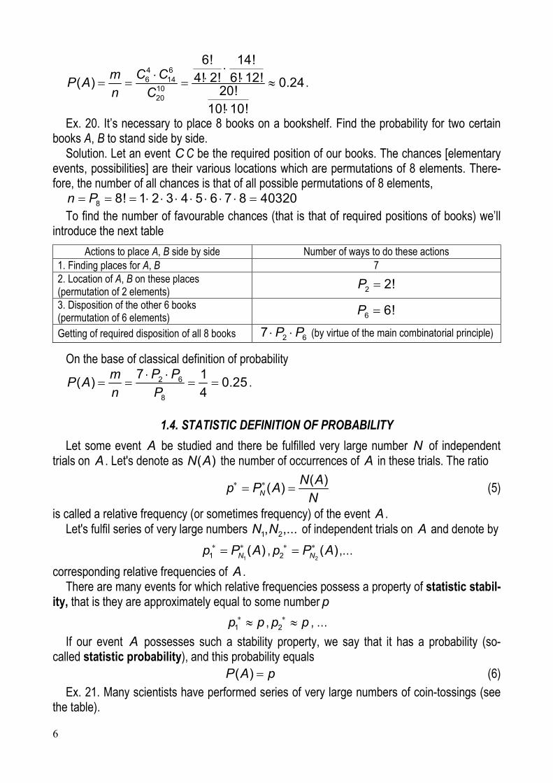
Ex. 21. Many scientists have performed series of very large numbers of coin-tossings (see the table).

7

Scientist N N(“head”) ( )Np P A (“head”)

Buffon G.L.L. (1777) 4040 2048 0.507 de Morgan A.(at the beginning of the 19th century)

4092 2048 0.5005

Pearson K. (at the beginning of the 20th century)

12000 6019 0.5016

Pearson K. 24000 12012 0.50005

On the base of these results we conclude that the statistical probability of the event “head” (in one coin-tossing) equals p = P (“head”) = 0.5, that is coincides with its "classic" probability.

2. MAIN RULES OF EVALUATING PROBABILITIES

2.1. SUM AND PRODUCT OF EVENTS

Def. 1. Sum A B ( A or B ) of two events A and B is called an event which consists in occurrence of at least one of them [which means that at least one of these events occurs] ( A but not B or B but not A or A and B together).

Ex. 1. Sum of an event A and its opposite one A is a certain event. Ex. 2. If an event A is “1” in one dice rolling, then the opposite event A is the sum

"2" "3" "4" "5" "6"A . Def. 2. Product AB ( A and B ) of two events A and B is called an event consisting in

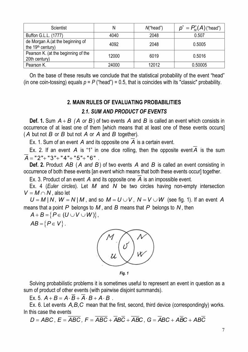
occurrence of both these events [an event which means that both these events occur] together. Ex. 3. Product of an event A and its opposite one A is an impossible event. Ex. 4 (Euler circles). Let M and N be two circles having non-empty intersection

V M N , also let |U M N , |W N M , and so M U V , N V W (see fig. 1). If an event A

means that a point P belongs to M , and B means that P belongs to N , then ( )A B P U V W ,

AB P V .

Fig. 1

Solving probabilistic problems it is sometimes useful to represent an event in question as a sum of product of other events (with pairwise disjoint summands).

Ex. 5. A B A B A B A B . Ex. 6. Let events , ,A B C mean that the first, second, third device (correspondingly) works.

In this case the events D ABC , E ABC , F ABC ABC ABC , G ABC ABC ABC

8

F G D E mean respectively that all the three devices work, none device works, only one device works (and the other two don’t work), two devices work (and one doesn’t work), at least one device works.

2.2. AXIOMS OF PROBABILITY THEORY. COROLLARIES

We state axioms of the probability theory on the base of statistic definition of probability ( ( ) ( )NP A P A for a large number N of trials).

1. If A is an impossible event, then its probability equals zero, ( ) 0P A ( A is impossible). 2. If A is a certain event, then its probability equals unity, ( ) 1P A ( A is certain). 3. If A is a random event, then its probability is contained between zero and unity,

0 ( ) 1P A ( A is random). 4. If A and B are two disjoint events, then the probability of their sum is equal to the sum

of probabilities of these events, P A B P A P B ( A ,B are disjoint). To formulate the last axiom let’s introduce the notion of a conditional probability of an

event. Namely, /P B A is the probability of an event B by condition that an event A oc-curs. Analogous is the probability of A if B occurs.

5. Probability of a product of two events equals the product of the probability of one event and the condition probability of the other, / ( ) /P AB P A P B A P B P A B .

Ex. 7. An urn contains 3 white and 2 black balls. One takes two balls successively and at random. Find the probability that they are white.

Solution. Let's denote by A an event which means that two drawn balls are white. Also let's denote by B and C events which mean that the first and the second drawn balls are white respectively. It's evident that A BC , hence, by virtue of the fifth axiom (and classic definition of probability)

3 2/ ( ) / 0.3

5 4P BC P B P C B P C P B C .

Some corollaries 1. If some events , ,A B C are pairwise disjoint, then P A B C P A P B P C . If, moreover, they form a total group, then

1P A B C P A P B P C . 2. The sum of probabilities of two opposite events equals 1,

1P A P A

because the events A , A are disjoint and form a total group. 3. Probabilities of a product of three, four etc events are equal to

/ /P ABC P A P B A P C AB 4. For two arbitrary events A and B the probability of their sum equals

P A B P A P B P AB . Def 3. Two events A ,B are called independent if probability of one of them doesn’t depend

on occurrence (or non-occurrence) of the other. For 3, 4 … events one introduces a notion of mutual independence (independence in the

aggregate, collectionwise independence).

9

Def 4. n events (for 2n ) are called mutually independent if the probability of one of them doesn’t depend on occurrence or non-occurrence of any group of the other.

5. If A , B are independent events, then / ( )P B A P B , / ( )P A B P A and so

P AB P A P B , that is the probability of a product of two independent events is equal to the product of their probabilities.

6. If , ,A B C are mutually independent events, then ( )P ABC P A P B P C

Ex. 8. To pass an exam successfully a student has to know the proofs of 50 theorems but he knows only 40 of them. What is the probability for him to pass an exam if exam tasks con-tain 3 theorems?

Solution. Let A be an event which means that a student will pass an exam. Let’s introduce the next three auxiliary events: 1B that is a student knows the proof of the first theorem, 2B of the second, 3B of the third. Then by the fourth corollary (and classic definition of probability)

1 2 3 1 2 3 1 2 1 3 1 2( ) ( ) ( ) ( / ) ( / )A B B B P A P B B B P B P B B P B B B 40 39 38

( ) 0.550 49 48

P A .

Ex. 9. A device consists of 2 independent modules. Probability for these modules to work are 0.95 and 0.9 respectively. Find the probability that the device doesn’t work because of: a) only one module; b) at least one module.

Solution. Let an event A mean that a device doesn’t work because of only one module, and an event B because of at least one module. Let events 1C , 2C mean that the first, the second module works. By condition

1( ) 0.95P C , 2( ) 0.9P C and so by the corollary 3

1 1( ) 1 ( ) 1 0.95 0.05P C P C , 2 2( ) 1 ( ) 1 0.9 0.1P C P C

We represent the events A ,B and B as follows

1 2 1 2A C C C C , 1 2 1 2 1 2 1 2B C C C C C C B C C . All summands are pairwise disjoint, and all factors are independent in summands. Therefore,

1 2 1 2 1 2 1 2( ) ( ) ( ) ( ) 0.05 0.9 0.1 0.95 0.14P A P C C C C P C C P C C

1 2( ) ( ) 0.95 0.9 0.86P B P C C ( ) 1 ( ) 1 0.86 0.14P B P B . Ex. 10. Three independently working engines are installed in a workshop. Probabilities to

work at a given time equal for them 0.6, 0.9, 0.7 respectively. Find probabilities of the next events: a) only one engine works; b) at least one engine works.

Solution. Let an event A mean that only one engine works and an event B mean that at least one engine works. Our problem is to find the probabilities of these events.

Let’s introduce three auxiliary events, namely 1C which means that the first engine works,

2C the second engine works and 3C the third engine works. By conditions of the problem

1( ) 0.6P C , 1 1( ) 1 ( ) 1 0.6 0.4P C P C

10

2( ) 0.9P C , 2 2( ) 1 ( ) 1 0.9 0.1P C P C

3( ) 0.7P C , 3 3( ) 1 ( ) 1 0.7 0.3P C P C a) The event A can be represented as the sum of products

1 2 3 1 2 3 1 2 3A C C C C C C C C C with pairwise disjoint summands and independent factors in every summand. Hence the prob-ability of the event A equals

1 2 3 1 2 3 1 2 3 1 2 3 1 2 3 1 2 3( ) ( ) ( ) ( ) ( )P A P C C C C C C C C C P C C C P C C C P C C C ( ) 0.6 0.1 0.3 0.4 0.9 0.3 0.4 0.1 0.7 0.154P A .

b) To find the probability of the eventB we’ll evaluate at first the probability of its opposite one B (which means that all three engines don't work, 1 2 3B C C C ).

We’ll obtain

1 2 3( ) ( ) 0.4 0.1 0.3 0.012P B P C C C whence it follows that

( ) 1 ( ) 1 0.012 0.988P B P B .

2.3. FORMULAE OF TOTAL PROBABILITY AND BAYES

The formula of total probability In practice we often deal with the next situation. An event A can occur only together with

one of pairwise disjoint events 1 2, , ..., nH H H , which form a total group. Let's call these events hypotheses. Their probabilities and corresponding conditional prob-

abilities of the event A are known. In this case the probability of the event A can be found with the help of the next formula (the formula of total probability):

1 1 2 2/ / ... /n nP A P H P A H P H P A H P H P A H (4)

( 1 2 ... 1nP H P H P H ) Bayes formulae Let an event A , which can occur only together with one of given hypotheses

1 2, , ..., nH H H , occur. In this case the next probabilities /kP H A of its occurrence togeth-er with each of these hypotheses can be evaluated with the help of the known Bayes formulas

/

/ , 1,k kk

P H P A HP H A k n

P A. (5)

Bayes formulae (5) state the probability that namely the k -th hypothesis has occurred to-gether with the event A in question.

Ex. 11. There are 6 white and 2 black balls in the first urn and 8 white and 3 black balls in the second urn. One moves a ball from the first urn to the second one at random, and then he takes a ball from the second urn (also at random).

1. Find the probability for him to take a white ball from the second urn. 2. Let a white ball be taken from the second urn. A ball of which colour was most probably

moved from the first urn? 1. Solution of the first problem. Let an event A mean that one will take a white ball from the

second urn. We can introduce the next two hypotheses: 1H means that one has moved a white ball from the first urn; 2H that he has moved a black ball from there. Their probabilities equal

11

1 2

6 3 2 1;

8 4 8 4P H P H

by condition, and corresponding conditional probabilities of the event A equal

1 2

9 3 8 2/ ; / .

12 4 12 3P A H P A H

On the base of the formula (4) of total probability the probability of the event A equals

1 1 2 2

3 3 1 2/ / 0.73.

4 4 4 3P A P H P A H P H P A H

2. To solve the second problem we must find and compare the next conditional probabili-ties 1 /P H A , 2 /P H A . On the base of Bayes formulae (5)

1 11

3 3/ 4 4/ 0.77

0,73

P H P A HP H A

P A

2 22

1 2/ 4 3/ 0,23.

0,73

P H P A HP H A

P A

We see that 0.77 > 0.23, therefore one has the most probably moved a white ball from the first urn to the second one.

Ex. 12. There are 10 and 15 products of the first and second factories respectively in the storage. The first factory makes 5% and the second 7% of defective products. One takes a product at random.

1) Find the probability of its defectiveness. 2) Suppose that this product is defective. Which factory has most probably made it? Solution. Let an event A mean that a product taken at random is defective. Let's introduce

the next two hypotheses: 1H this product was done by the first factory; 2H it was done by the second factory.

On the base of the classical definition of probability

1 2

10 150.4; 0.6

25 25P H P H .

Corresponding conditional probabilities of the event A equal

1 2

5 7/ 0.05; / 0.07.

100 100P A H P A H

1) Using the formula of total probability we'll get 1 1 2 2/ / 0.4 0.05 0.6 0.07 0.062.P A P H P A H P H P A H

2) Now with the help of Bayes formulas we find

1 11

/ 0.4 0.05/ 0.32

0,062

P H P A HP H A

P A

2 22

/ 0.6 0.07/ 0,68.

0,062

P H P A HP H A

P A

Thus, 2 1/ /P H A P H A

Therefore, the taken product was most probably made by the second factory.

12

Exercise Set 1, 2. 1. The first worker makes 40% of the second-class parts, and the second makes 30%. Two

parts are taken from each worker at random. Find the probability that: a) all the four parts are second-class; b) at least three parts are second-class; c) less than three parts are second-class.

2. A worker services three machine tools. The probability that during his shift the machine tools will claim his attention is equal to 0.7 for the first one, 0.65 for the second one, 0.55 for the third one. Find the probability that during his shift his attention will be claimed by: a) two machine tools; b) not less than two machine tools; c) at least one machine tool.

3. The probability that the student will pass the examinations is equal to 0.8 for the first one, 0.7 for the second one, 0.65 for the third one. Find the probability that the student will pass: a) two examinations; b) not less than two examinations; c) at least one examination.

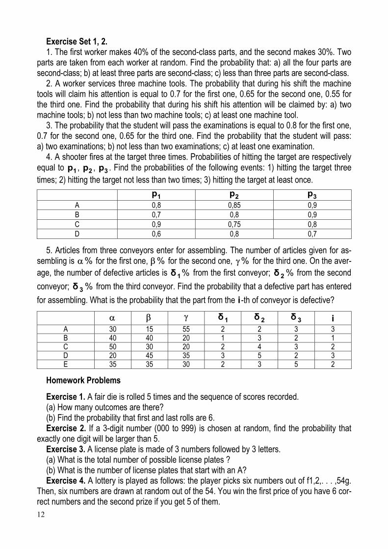
4. A shooter fires at the target three times. Probabilities of hitting the target are respectively equal to 1p , 2p , 3p . Find the probabilities of the following events: 1) hitting the target three times; 2) hitting the target not less than two times; 3) hitting the target at least once.

1p 2p 3p

A 0,8 0,85 0,9 B 0,7 0,8 0,9 C 0,9 0,75 0,8 D 0,6 0,8 0,7

5. Articles from three conveyors enter for assembling. The number of articles given for as-sembling is % for the first one, % for the second one, % for the third one. On the aver-age, the number of defective articles is %1δ from the first conveyor; %2δ from the second

conveyor; %3δ from the third conveyor. Find the probability that a defective part has entered

for assembling. What is the probability that the part from the i -th of conveyor is defective?

1δ 2δ 3δ i A 30 15 55 2 2 3 3 B 40 40 20 1 3 2 1 C 50 30 20 2 4 3 2 D 20 45 35 3 5 2 3 E 35 35 30 2 3 5 2

Homework Problems

Exercise 1. A fair die is rolled 5 times and the sequence of scores recorded. (a) How many outcomes are there? (b) Find the probability that first and last rolls are 6. Exercise 2. If a 3-digit number (000 to 999) is chosen at random, find the probability that

exactly one digit will be larger than 5. Exercise 3. A license plate is made of 3 numbers followed by 3 letters. (a) What is the total number of possible license plates ? (b) What is the number of license plates that start with an A? Exercise 4. A lottery is played as follows: the player picks six numbers out of f1,2,. . . ,54g.

Then, six numbers are drawn at random out of the 54. You win the first price of you have 6 cor-rect numbers and the second prize if you get 5 of them.

13

(a) What is the probability to win the first prize ? (b) What is the probability to win the second prize ? Exercise 5. Another lottery is played as follows: the player picks five numbers out of

f1,2,. . . ,50g and two other numbers from the list f1,. . . ,9g. Then, five numbers are drawn at random from the first list and two from the random list.

(a) You win the first prize if all numbers are correct. What is the probability to win the first prize ? (b) Which lottery would you choose to play between this one and the one from the previous

problem ? Exercise 6. An urn contains 3 red, 8 yellow and 13 green balls; another urn contains 5 red,

7 yellow and 6 green balls. We pick one ball from each urn at random. Find the probability that both balls are of the same color.

Exercise 7. Suppose that there are 5 duck hunters, each a perfect shot. A flock of 10 ducks fly over, and each hunter selects one duck at random and shoots. Find the probability that 5 ducks are killed.

Exercise 8. A conference room contains m men and w women. These people seat at ran-dom in m + w seats arranged in a row. Find the probability that all the women will be adjacent.

Exercise 9. If a box contains 75 good light bulbs and 25 defective bulbs and 15 bulbs are removed, find the probability that at least one will be defective.

Exercise 10. Find the probability that a five-card poker hand (i.e. 5 out of a 52-card deck) will be :

(a) Four of a kind, that is four cards of the same value and one other card of a different val-ue (xxxxy shape).

(b) Three of a kind, that is three cards of the same value and two other cards of different values (xxxyz shape).

(c) A straight flush, that is five cards in a row, of the same suit (ace may be high or low). (d) A flush, that is five cards of the same suit, but not a straight flush. (e) A straight, that is five cards in a row, but not a straight flush (ace may be high or low). Exercise 11. An urn contains 10 balls numbered from 1 to 10. We draw five balls from the

urn, without replacement. Find the probability that the second largest number drawn is 8. Exercise 12. Eight cards are drawn without replacement from an ordinary deck. Find the

probability of obtaining exactly three aces or exactly three kings (or both). Exercise 13. How many possible ways are there to seat 8 people (A,B,C,D,E,F,G and H) in

a row, if: (a) No restrictions are enforced; (b) A and B want to be seated together; (c) assuming there are four men and four women, men should be only seated between

women and the other way around; (d) assuming there are five men, they must be seated together; (e) assuming these people are four married couples, each couple has to be seated together. Exercise 14. John owns six discs: 3 of classical music, 2 of jazz and one of rock (all of

them different). How many possible ways does John have if he wants to store these discs on a shelf, if:

(a) No restrictions are enforced; (b) The classical discs and the jazz discs have to be stored together; (c) The classical discs have to be stored together, but the jazz discs have to be separated.

14

Exercise 15. How many (not necessarily meaningful) words can you form by shuffling the letters of the following words: (a) bike; (b) paper; (c) letter; (d) minimum.

Exercise 16. An urn contains 30 white and 15 black balls. If 10 balls are drawn with (re-spectively without) replacement, find the probability that the first two balls will be white, given that the sample contains exactly six white balls.

Exercise 17. In a certain village, 20% of the population has some disease. A test is admin-istered which has the property that if a person is sick, the test will be positive 90% of the time and if the person is not sick, then the test will still be positive 30% of the time. All people tested positive are prescribed a drug which always cures the disease but produces a rash 25% of the time. Given that a random person has the rash, what is the probability that this person had the disease to start with?

Exercise 18. An insurance company considers that people can be split in two groups : those who are likely to have accidents and those who are not. Statistics show that a person who is likely to have an accident has probability 0.4 to have one over a year; this probability is only 0.2 for a person who is not likely to have an accident. We assume that 30% of the popula-tion is likely to have an accident.

(a) What is the probability that a new customer has an accident over the first year of his contract?

(b) A new customer has an accident during the first year of his contract. What is the proba-bility that he belongs to the group likely to have an accident?

Exercise 19. A transmitting system transmits 0’s and 1’s. The probability of a correct transmission of a 0 is 0.8, and it is 0.9 for a 1. We know that 45% of the transmitted symbols are 0’s.

(a) What is the probability that the receiver gets a 0? (b) If the receiver gets a 0, what is the probability the transmitting system actually sent a 0? Exercise 20. 46% of the electors of a town consider themselves as independent, whereas

30% consider themselves democrats and 24% republicans. In a recent election, 35% of the independents, 62% of the democrats and 58% of the republicans voted.

(a) What proportion of the total population actually voted? (b) A random voter is picked. Given that he voted, what is the probability that he is inde-

pendent? democrat? republican?

3. RANDOM VARIABLES

3.1. A RANDOM VARIABLE

Def. 1. A random variable is a variable which takes on some value in any trial and this value isn’t known beforehand [in advance].

We’ll denote random variables by letters , , ,...X Y Z and their possible values by x, y, z, … . We’ll study discrete and continuous random variables.

Def. 2. A random variable is called discrete if it can take on only separate isolated possible values (with some probabilities).

Ex.1. A number X of occurrences of an event A in one trial: 1X if A occurs, and 0X , if A doesn’t occur (that is an opposite event A occurs);

( 1) ( )P X P A , ( 0) ( ) 1 ( )P X P A P A

15

Ex. 2. The number of students on the lecture. Ex. 3. The daily production of some factory (in items). Definition of a continuous random variable will be given below. Now we’ll only say that its

possible values fill some interval completely. Ex. 4. The human height and weight. Ex. 5. The size of an item. Ex.6.The error of measurement. Def. 3. The distribution [the distribution law, the law of distribution, the law] of a random var-

iable is a rule which sets a correspondence between its possible values and corresponding probabilities.

The distribution law of a random variable can be expressed: 1) analytically by a formula (for example ( ) , 1m m n m

n nP X m C p q q p ); 2) tabularly (by the distribution table for discrete random variables); 3) geometrically (by distribution polygon for discrete random variables, by graph of the

distribution function or density (see below)). The distribution table of a discrete random variable X (with finite number n of possible

values) has the next form:

X 1x 2x … nx

P 1p 2p … np

Its first row contains all possible values of the random variable, and the second row contains corresponding probabilities of these values. The notation iX x means that the random vari-able X takes on a value ix . Events

1( )X x , 2( )X x ,…,( )nX x are pairwise disjoint and form a total group. Therefore, the sum of their probabilities

1 1( )p P X x , 2 2( )p P X x ,…, ( )n np P X x equals 1( 1 ip ).

Fig. 2

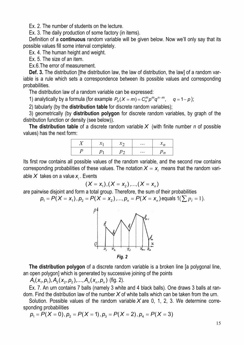
The distribution polygon of a discrete random variable is a broken line [a polygonal line, an open polygon] which is generated by successive joining of the points

1 1 1 2 2 2( , ), ( , ),..., ( , )n n nA x p A x p A x p (fig. 2). Ex. 7. An urn contains 7 balls (namely 3 white and 4 black balls). One draws 3 balls at ran-

dom. Find the distribution law of the number X of white balls which can be taken from the urn. Solution. Possible values of the random variable X are 0, 1, 2, 3. We determine corre-

sponding probabilities

1 ( 0)p P X , 2 ( 1)p P X , 3 ( 2)p P X , 4 ( 3)p P X

16

with the help of the classical definition of probability. Elementary events (chances) for every of these four cases are sets of 3 balls that is 3-fold combinations of 7 elements. Hence the gen-eral number of chances equals

37

7!35

3! 4!n C

.

Numbers of favourable chances are represented in the table

Event Number of favorable chances Explication

0X 3 11 4 4 4m C C

One can take 0 white (and so 3 black) balls by the number of 3-fold combinations of 4 elements

1X 2

2 43 18m C One can take 1 white ball by 3 ways and 2 black balls by 24C ways

2X 2

3 34 12m C One can take 2 white balls by 23C ways and 1 black ball by 4 ways

3X 4 1m One can take 3 white balls in one unique way

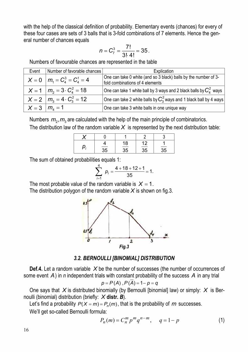
Numbers 2 3,m m are calculated with the help of the main principle of combinatorics. The distribution law of the random variable X is represented by the next distribution table:

X 0 1 2 3

ip 4

35

18

35

12

35

1

35

The sum of obtained probabilities equals 1: 4

1

4 18 12 11

35i

i

p

.

The most probable value of the random variable is 1X . The distribution polygon of the random variable X is shown on fig.3.

Fig.3

3.2. BERNOULLI [BINOMIAL] DISTRIBUTION

Def.4. Let a random variable X be the number of successes (the number of occurrences of some event A ) in n independent trials with constant probability of the success A in any trial

( )p P A , ( ) 1P A p q One says that X is distributed binomially (by Bernoulli [binomial] law) or simply: X is Ber-

noulli (binomial) distribution (briefly: X distr. B). Let’s find a probability ( ) ( )nP X m P m , that is the probability of m successes. We’ll get so-called Bernoulli formula:

pqqpCmP mnmmnn 1,)( (1)

17

Note 1. For 0,1,2,...m the value of the probability (1) first increases and then decreases, and therefore there exists the so-called most probable number 0m of successes.

It is defined by the next double inequality pnpmqnp 0 , max)( 0 mPn (2)

Note 2. Probability of no less than 1k and no greater than 2k successes equals )(...)2()1()()( 211121 kPkPkPkPkmkP nnnnn (3)

Ex. 8. 6 independently working engines are installed in a shop. Probability for any engine to work at a given moment is 0.8. Find the distribution of a random variable X which is a number of working engines at this moment. Find the probabilities of at least one engine to work, of no less than 2 and no greater than 5 engines to work and the most probable value of X .

Solution. We can consider setting of an engine as a trial. So we have n = 6 independent tri-als. Let a success A mean that an engine works.

( ) 0.8p P A , ( ) 1 0.2P A p q The random variable X has Bernoulli distribution (briefly “ X distributed B”), it can take on

the values 0,1,2,3,4,5,6, which one calculates by Bernoulli formula (1). For example 0 0 6 6

6 6( 0) (0) 0.2 0.00006P X P C p q 1 1 5 5

6 6( 1) (1) 6 0.8 0.2 0.00154P X P C p q By the same way the other probabilities are calculated, and the distribution table of the ran-

dom variable is the next one

X 0 1 2 3 4 5 6

ip 0.00006 0.00154 0.01536 0.08192 0.24576 0.39321 0.26214

The probability of at least one engine to work equals 6( 0) ( 1) 1 ( 0) 1 0.99994P X P X P X q

The most probable value of X , 0 5m , we see in the table. Evaluation of 0m by the for-mula (2) gives 0 06 0.8 0.2 6 0.8 0.8np q m np p m whence it follows that

0 04.6 5.6 5m m . Probability of no less than 2 and no greater than 5 engines to work on the base of the for-

mula (3) equals 6 6 6 6 6(2 5) (2) (3) (4) (5)P m P P P P = 0.01536 + 0.08192+ 0.24576 + 0.39321 + 0.73625 0.74

Bernoulli formula (1) isn’t convenient for large number n of trials. There are some approxi-mate formulas.

3.3. POISSON FORMULA AND DISTRIBUTION

Let a random variable X be distributed B . Let’s suppose that the number n of trials tends to infinity, the probability p of a success A goes to zero, but a product np retains constant,

, 0,n p np const . In this case the limit of the probability ( ) ( )nP X m P m , which is defined by Bernoulli formula (1), equals

em

mPm

n !)( (4)

18

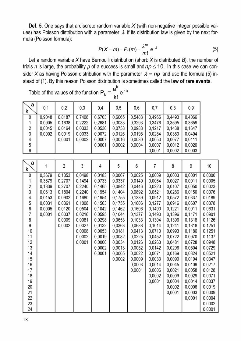
Def. 5. One says that a discrete random variable X (with non-negative integer possible val-ues) has Poisson distribution with a parameter if its distribution law is given by the next for-mula (Poisson formula):

( ) ( )!

m

nP X m P m em

(5)

Let a random variable X have Bernoulli distribution (short: X is distributed B), the number of trials n is large, the probability p of a success is small and 10np . In this case we can con-sider X as having Poisson distribution with the parameter np and use the formula (5) in-stead of (1). By this reason Poisson distribution is sometimes called the law of rare events.

Table of the values of the function k

ak

aP = e

k!-

a k

0,1 0,2 0,3 0,4 0,5 0,6 0,7 0,8 0,9

0 1 2 3 4 5 6

0,9048 0,0905 0,0045 0,0002

0,8187 0,1638 0,0164 0,0019 0,0001

0,7408 0,2222 0,0333 0,0033 0,0002

0,6703 0,2681 0,0536 0,0072 0,0007 0,0001

0,6065 0,3033 0,0758 0,0126 0,0016 0,0002

0,5488 0,3293 0,0988 0,0198 0,0030 0,0004

0,4966 0,3476 0,1217 0,0284 0,0050 0,0007 0,0001

0,4493 0,3595 0,1438 0,0383 0,0077 0,0012 0,0002

0,4066 0,3659 0,1647 0,0494 0,0111 0,0020 0,0003

a

k 1 2 3 4 5 6 7 8 9 10

0 1 2 3 4 5 6 7 8 9 10 11 12 13 14 15 16 17 18 19 20 21 22 23 24

0,3679 0,3679 0,1839 0,0613 0,0153 0,0031 0,0005 0,0001

0,1353 0,2707 0,2707 0,1804 0,0902 0,0361 0,0120 0,0037 0,0009 0,0002

0,0498 0,1494 0,2240 0,2240 0,1680 0,1008 0,0504 0,0216 0,0081 0,0027 0,0008 0,0002 0,0001

0,0183 0,0733 0,1465 0,1954 0,1954 0,1563 0,1042 0,0595 0,0298 0,0132 0,0053 0,0019 0,0006 0,0002 0,0001

0,0067 0,0337 0,0842 0,1404 0,1755 0,1755 0,1462 0,1044 0,0653 0,0363 0,0181 0,0082 0,0034 0,0013 0,0005 0,0002

0,0025 0,0149 0,0446 0,0892 0,1339 0,1606 0,1606 0,1377 0,1033 0,0688 0,0413 0,0225 0,0126 0,0052 0,0022 0,0009 0,0003 0,0001

0,0009 0,0064 0,0223 0,0521 0,0912 0,1277 0,1490 0,1490 0,1304 0,1014 0,0710 0,0452 0,0263 0,0142 0,0071 0,0033 0,0014 0,0006 0,0002 0,0001

0,0003 0,0027 0,0107 0,0286 0,0572 0,0916 0,1221 0,1396 0,1396 0,1241 0,0993 0,0722 0,0481 0,0296 0,0169 0,0090 0,0045 0,0021 0,0009 0,0004 0,0002 0,0001

0,0001 0,0011 0,0050 0,0150 0,0337 0,0607 0,0911 0,1171 0,1318 0,1318 0,1186 0,0970 0,0728 0,0504 0,0324 0,0194 0,0109 0,0058 0,0029 0,0014 0,0006 0,0003 0,0001

0,0000 0,0005 0,0023 0,0076 0,0189 0,0378 0,0631 0,0901 0,1126 0,1251 0,1251 0,1137 0,0948 0,0729 0,0521 0,0347 0,0217 0,0128 0,0071 0,0037 0,0019 0,0009 0,0004 0,0002 0,0001

19

Ex. 9. 500 items are sent. Probability of damage of an item in the trade is 0.002. Find the probabilities: a) 3, b) less than 3, c) more than 2 items are damaged; d) at least one item is damaged.

Solution. We have 500n independent trials, a success A is a damage of an item, ( ) 0.002p P A const , a random variable X is a number of damaged items. X is dis-

tributed B , but n is large, p is small, 1np . Therefore we can consider X as Poisson dis-tribution with 1 and make use of Poisson formula (5).

a) ( 3) 0.0613P X b) ( 3) ( 2) ( 0) ( 1) ( 2) 0.3679 0.3679 0.1839 0.9197P X P X P X P X P X c) ( 2) 1 ( 2) 1 0.9197 0.0803P X P X d) ( 1) ( 0) 1 ( 0) 1 0.3679 0.6321P X P X P X .

3.4 LAPLACE LOCAL AND INTEGRAL THEOREMS

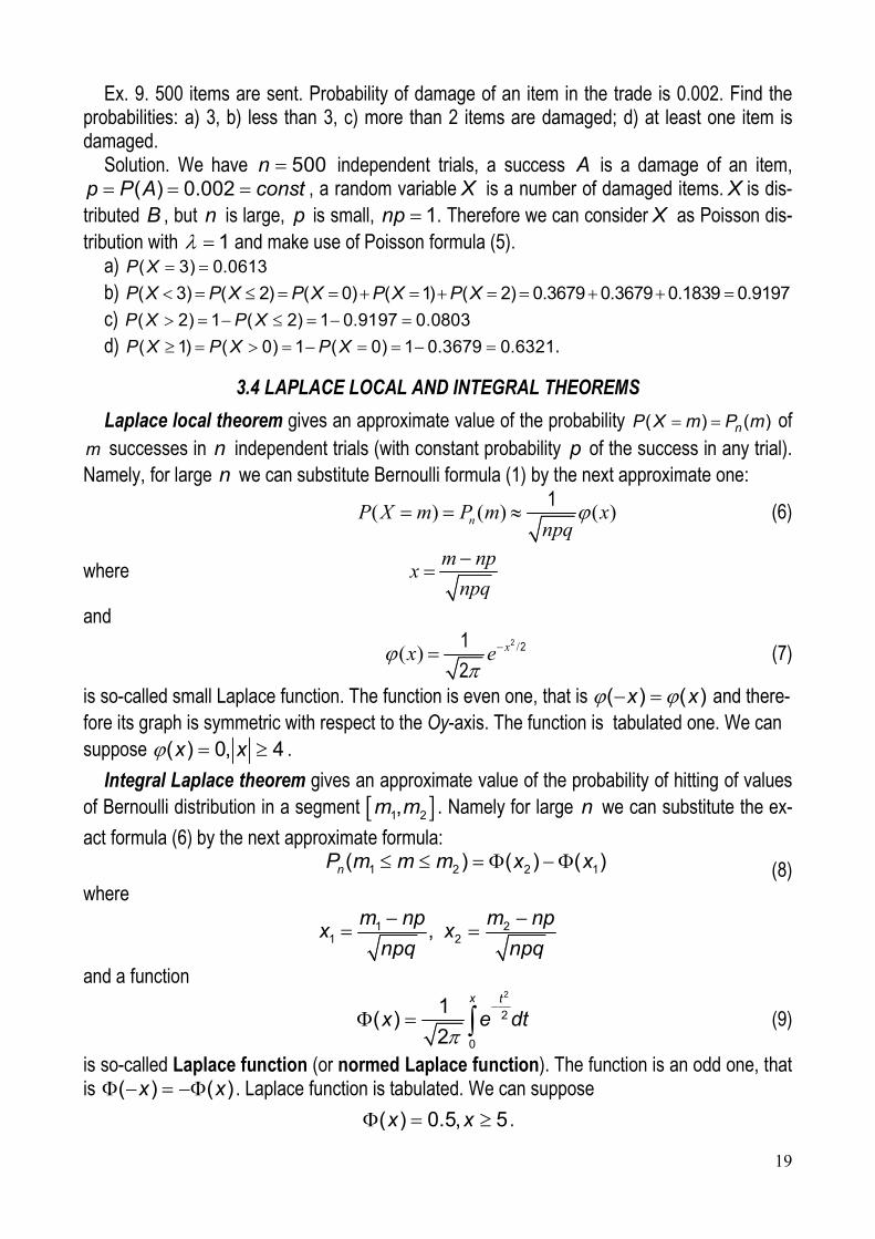
Laplace local theorem gives an approximate value of the probability ( ) ( )nP X m P m of m successes in n independent trials (with constant probability p of the success in any trial). Namely, for large n we can substitute Bernoulli formula (1) by the next approximate one:

( ) ( ) ( )nP X m P m xnpq

1

(6)

where

m np

xnpq

and /( ) xx e

2 21

2 (7)

is so-called small Laplace function. The function is even one, that is ( ) ( )x x and there-fore its graph is symmetric with respect to the Oy-axis. The function is tabulated one. We can suppose ( ) 0, 4x x .

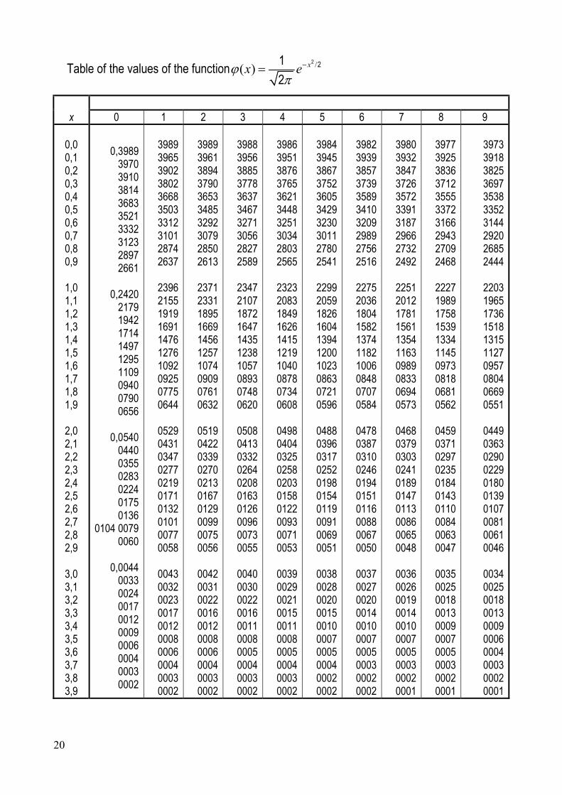
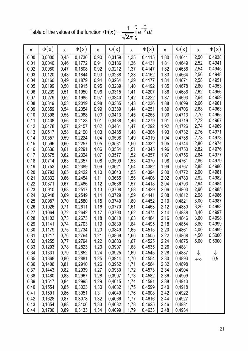
Integral Laplace theorem gives an approximate value of the probability of hitting of values of Bernoulli distribution in a segment 1 2,m m . Namely for large n we can substitute the ex-

act formula (6) by the next approximate formula: 1 2 2 1( ) ( ) ( )nP m m m x x (8)

where

1 21 2,

m np m npx x

npq npq

and a function

2

2

0

1( )

2

x t

x e dt (9)

is so-called Laplace function (or normed Laplace function). The function is an odd one, that is ( ) ( )x x . Laplace function is tabulated. We can suppose

( ) 0.5, 5x x .

20

Table of the values of the function /( )

xx e2 21

2

х 0 1 2 3 4 5 6 7 8 9

0,0 0,1 0,2 0,3 0,4 0,5 0,6 0,7 0,8 0,9

1,0 1,1 1,2 1,3 1,4 1,5 1,6 1,7 1,8 1,9

2,0 2,1 2,2 2,3 2,4 2,5 2,6 2,7 2,8 2,9

3,0 3,1 3,2 3,3 3,4 3,5 3,6 3,7 3,8 3,9

0,3989

3970 3910 3814 3683 3521 3332 3123 2897 2661

0,2420

2179 1942 1714 1497 1295 1109 0940 0790 0656

0,0540

0440 0355 0283 0224 0175 0136

0104 0079 0060

0,0044

0033 0024 0017 0012 0009 0006 0004 0003 0002

3989 3965 3902 3802 3668 3503 3312 3101 2874 2637

2396 2155 1919 1691 1476 1276 1092 0925 0775 0644

0529 0431 0347 0277 0219 0171 0132 0101 0077 0058

0043 0032 0023 0017 0012 0008 0006 0004 0003 0002

3989 3961 3894 3790 3653 3485 3292 3079 2850 2613

2371 2331 1895 1669 1456 1257 1074 0909 0761 0632

0519 0422 0339 0270 0213 0167 0129 0099 0075 0056

0042 0031 0022 0016 0012 0008 0006 0004 0003 0002

3988 3956 3885 3778 3637 3467 3271 3056 2827 2589

2347 2107 1872 1647 1435 1238 1057 0893 0748 0620

0508 0413 0332 0264 0208 0163 0126 0096 0073 0055

0040 0030 0022 0016 0011 0008 0005 0004 0003 0002

3986 3951 3876 3765 3621 3448 3251 3034 2803 2565

2323 2083 1849 1626 1415 1219 1040 0878 0734 0608

0498 0404 0325 0258 0203 0158 0122 0093 0071 0053

0039 0029 0021 0015 0011 0008 0005 0004 0003 0002

3984 3945 3867 3752 3605 3429 3230 3011 2780 2541

2299 2059 1826 1604 1394 1200 1023 0863 0721 0596

0488 0396 0317 0252 0198 0154 0119 0091 0069 0051

0038 0028 0020 0015 0010 0007 0005 0004 0002 0002

3982 3939 3857 3739 3589 3410 3209 2989 2756 2516

2275 2036 1804 1582 1374 1182 1006 0848 0707 0584

0478 0387 0310 0246 0194 0151 0116 0088 0067 0050

0037 0027 0020 0014 0010 0007 0005 0003 0002 0002

3980 3932 3847 3726 3572 3391 3187 2966 2732 2492

2251 2012 1781 1561 1354 1163 0989 0833 0694 0573

0468 0379 0303 0241 0189 0147 0113 0086 0065 0048

0036 0026 0019 0014 0010 0007 0005 0003 0002 0001

3977 3925 3836 3712 3555 3372 3166 2943 2709 2468

2227 1989 1758 1539 1334 1145 0973 0818 0681 0562

0459 0371 0297 0235 0184 0143 0110 0084 0063 0047

0035 0025 0018 0013 0009 0007 0005 0003 0002 0001

3973 3918 3825 3697 3538 3352 3144 2920 2685 2444

2203 1965 1736 1518 1315 1127 0957 0804 0669 0551

0449 0363 0290 0229 0180 0139 0107 0081 0061 0046

0034 0025 0018 0013 0009 0006 0004 0003 0002 0001

21

Table of the values of the function

2

2

0

1( )

2

x t

x e dt

x Φ x x Φ x x Φ x x Φ x x Φ x x Φ x

0,00 0,01 0,02 0,03 0,04 0,05 0,06 0,07 0,08 0,09 0,10 0,11 0,12 0,13 0,14 0,15 0,16 0,17 0,18 0,19 0,20 0,21 0,22 0,23 0,24 0,25 0,26 0,27 0,28 0,29 0,30 0,31 0,32 0,33 0,34 0,35 0,36 0,37 0,38 0,39 0,40 0,41 0,42 0,43 0,44

0,0000 0,0040 0,0080 0,0120 0,0160 0,0199 0,0239 0,0279 0,0319 0,0359 0,0398 0,0438 0,0478 0,0517 0,0557 0,0596 0,0636 0,0675 0,0714 0,0753 0,0793 0,0832 0,0871 0,0910 0,0948 0,0987 0,1026 0,1064 0,1103 0,1141 0,1179 0,1217 0,1255 0,1293 0,1331 0,1368 0,1406 0,1443 0,1480 0,1517 0,1554 0,1591 0,1628 0,1654 0,1700

0,45 0,46 0,47 0,48 0,49 0,50 0,51 0,52 0,53 0,54 0,55 0,56 0,57 0,58 0,59 0,60 0,61 0,62 0,63 0,64 0,65 0,66 0,67 0,68 0,69 0,70 0,71 0,72 0,73 0,74 0,75 0,76 0,77 0,78 0,79 0,80 0,81 0,82 0,83 0,84 0,85 0,86 0,87 0,88 0,89

0,1736 0,1772 0,1808 0,1844 0,1879 0,1915 0,1950 0,1985 0,2019 0,2054 0,2088 0,2123 0,2157 0,2190 0,2224 0,2257 0,2291 0,2324 0,2357 0,2389 0,2422 0,2454 0,2486 0,2517 0,2549 0,2580 0,2611 0,2642 0,2673 0,2703 0,2734 0,2764 0,2794 0,2823 0,2852 0,2881 0,2910 0,2939 0,2967 0,2995 0,3023 0,3051 0,3078 0,3106 0,3133

0,90 0,91 0,92 0,93 0,94 0,95 0,96 0,97 0,98 0,99 1,00 1,01 1,02 1,03 1,04 1,05 1,06 1,07 1,08 1,09 1,10 1,11 1,12 1,13 1,14 1,15 1,16 1,17 1,18 1,19 1,20 1,21 1,22 1,23 1,24 1,25 1,26 1,27 1,28 1,29 1,30 1,31 1,32 1,33 1,34

0,3159 0,3186 0,3212 0,3238 0,3264 0,3289 0,3315 0,3340 0,3365 0,3389 0,3413 0,3438 0,3461 0,3485 0,3508 0,3531 0,3554 0,3577 0,3599 0,3621 0,3643 0,3665 0,3686 0,3708 0,3729 0,3749 0,3770 0,3790 0,3810 0,3830 0,3849 0,3869 0,3883 0,3907 0,3925 0,3944 0,3962 0,3980 0,3997 0,4015 0,4032 0,4049 0,4066 0,4082 0,4099

1,35 1,36 1,37 1,38 1,39 1,40 1,41 1,42 1,43 1,44 1,45 1,46 1,47 1,48 1,49 1,50 1,51 1,52 1,53 1,54 1,55 1,56 1,57 1,58 1,59 1,60 1,61 1,62 1,63 1,64 1,65 1,66 1,67 1,68 1,69 1,70 1,71 1,72 1,73 1,74 1,75 1,76 1,77 1,78 1,79

0,4115 0,4131 0,4147 0,4162 0,4177 0,4192 0,4207 0,4222 0,4236 0,4251 0,4265 0,4279 0,4292 0,4306 0,4319 0,4332 0,4345 0,4357 0,4370 0,4382 0,4394 0,4406 0,4418 0,4429 0,4441 0,4452 0,4463 0,4474 0,4484 0,4495 0,4515 0,4505 0,4525 0,4535 0,4545 0,4554 0,4564 0,4573 0,4582 0,4591 0,4599 0,4608 0,4616 0,4625 0,4633

1,80 1,81 1,82 1,83 1,84 1,85 1,86 1,87 1,88 1,89 1,90 1,91 1,92 1,93 1,94 1,95 1,96 1,97 1,98 1,99 2,00 2,02 2,04 2,06 2,08 2,10 2,12 2,14 2,16 2,18 2,20 2,22 2,24 2,26 2,28 2,30 2,32 2,34 2,36 2,38 2,40 2,42 2,44 2,46 2,48

0,4641 0,4649 0,4656 0,4664 0,4671 0,4678 0,4686 0,4693 0,4699 0,4706 0,4713 0,4719 0,4726 0,4732 0,4738 0,4744 0,4750 0,4756 0,4761 0,4767 0,4772 0,4783 0,4793 0,4803 0,4812 0,4821 0,4830 0,4838 0,4846 0,4854 0,4861 0,4868 0,4875 0,4881 0,4887 0,4893 0,4898 0,4904 0,4909 0,4913 0,4918 0,4922 0,4927 0,4931 0,4934

2,50 2,52 2,54 2,56 2,58 2,60 2,62 2,64 2,66 2,68 2,70 2,72 2,74 2,76 2,78 2,80 2,82 2,84 2,86 2,88 2,90 2,92 2,94 2,96 2,98 3,00 3,20 3,40 3,60 3,80 4,00 4,50 5,00

0,4938 0,4941 0,4945 0,4948 0,4951 0,4953 0,4956 0,4959 0,4961 0,4963 0,4965 0,4967 0,4969 0,4971 0,4973 0,4974 0,4976 0,4977 0,4979 0,4980 0,4981 0,4982 0,4984 0,4985 0,4986 0,4987 0,4993 0,4997 0,4998 0,4999 0,4999 0,5000 0,5000

0,5

22

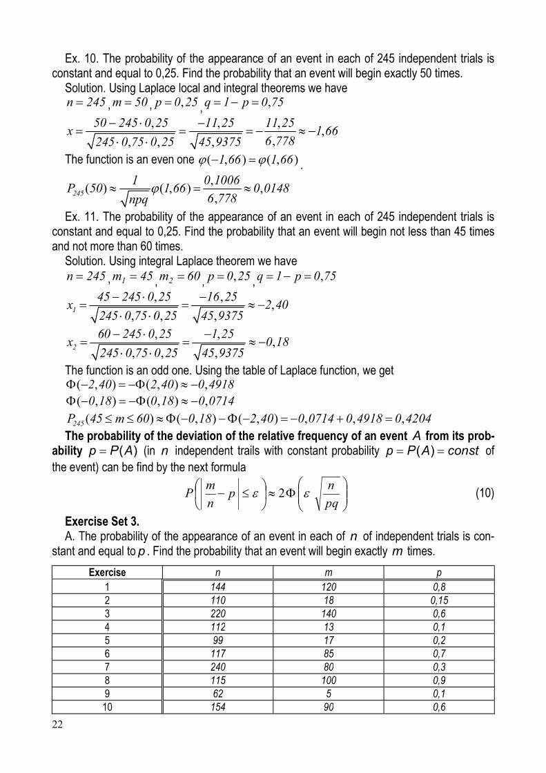
Ex. 10. The probability of the appearance of an event in each of 245 independent trials is constant and equal to 0,25. Find the probability that an event will begin exactly 50 times.

Solution. Using Laplace local and integral theorems we have 245n , 50m , ,p 0 25 , ,q 1 p 0 75

, , ,,

,, , ,

50 245 0 25 11 25 11 25x 1 66

6 778245 0 75 0 25 45 9375

The function is an even one ( , ) ( , )1 66 1 66 .

,( ) ( , ) ,

,245

1 0 1006P 50 1 66 0 0148

6 778npq

Ex. 11. The probability of the appearance of an event in each of 245 independent trials is

constant and equal to 0,25. Find the probability that an event will begin not less than 45 times and not more than 60 times.

Solution. Using integral Laplace theorem we have 245n , 45m1 , 60m2 , ,p 0 25 , ,q 1 p 0 75

, ,,

, , ,1

45 245 0 25 16 25x 2 40

245 0 75 0 25 45 9375

, ,

,, , ,

2

60 245 0 25 1 25x 0 18

245 0 75 0 25 45 9375

The function is an odd one. Using the table of Laplace function, we get

( , ) ( , ) ,2 40 2 40 0 4918 ( , ) ( , ) ,0 18 0 18 0 0714

( ) ( , ) ( , ) , , ,245P 45 m 60 0 18 2 40 0 0714 0 4918 0 4204 The probability of the deviation of the relative frequency of an event A from its prob-

ability ( )p P A (in n independent trails with constant probability ( )p P A const of the event) can be find by the next formula

pq

np

n

mP 2 (10)

Exercise Set 3. A. The probability of the appearance of an event in each of n of independent trials is con-

stant and equal to p . Find the probability that an event will begin exactly m times.

Exercise n m p 1 144 120 0,8 2 110 18 0,15 3 220 140 0,6 4 112 13 0,1 5 99 17 0,2 6 117 85 0,7 7 240 80 0,3 8 115 100 0,9 9 62 5 0,1 10 154 90 0,6

23

B. The probability of the appearance of an event in each of n of independent trials is con-stant and equal to p . Find the probability that an event will begin not less than 1m times and not more than 2m times.

Exercise n 1m 2m p 11 144 115 125 0,8 12 110 15 20 0,15 13 220 130 145 0,6 14 112 10 14 0,1 15 99 15 20 0,2 16 117 80 100 0,7 17 240 70 90 0,3 18 115 100 110 0,9 19 62 5 10 0,1 20 154 80 100 0,6

C. The probability of the production of a defective part is equal to p . Find the probability that from the tested n parts m are defective.

Exercise n m p 21 1000 6 0,008 22 2500 2 0,001 23 1500 10 0,006 24 3500 5 0,002 25 10000 4 0,0005 26 8000 6 0,0008 27 4500 5 0,0008 28 2000 1 0,0001 29 5000 3 0,0008 30 7000 4 0,0006

4. THE DISTRIBUTION FUNCTION AND DENSITY. NUMBER CHARACTERISTICS OF RANDOM VARIABLES

4.1. THE DISTRIBUTION FUNCTION OF A RANDOM VARIABLE

The distribution function is the most general form of the distribution law of a random variable X. Def. 1. The distribution function of a random variable X is called a function:

)()()( xPxPxF (1)

The distribution function ( )F x is the probability for the random variable X to take on val-ues which are less than x or the probability of hitting of the random variable in the infinite inter-val (the half-axis) ,x .

Properties of the distribution function 1. The distribution function, being a probability, lies between 0 and 1 [ranges from 0 to 1]:

1)(0 xF 2. 0)(lim

xF

x, 1)(lim

xF

x

24

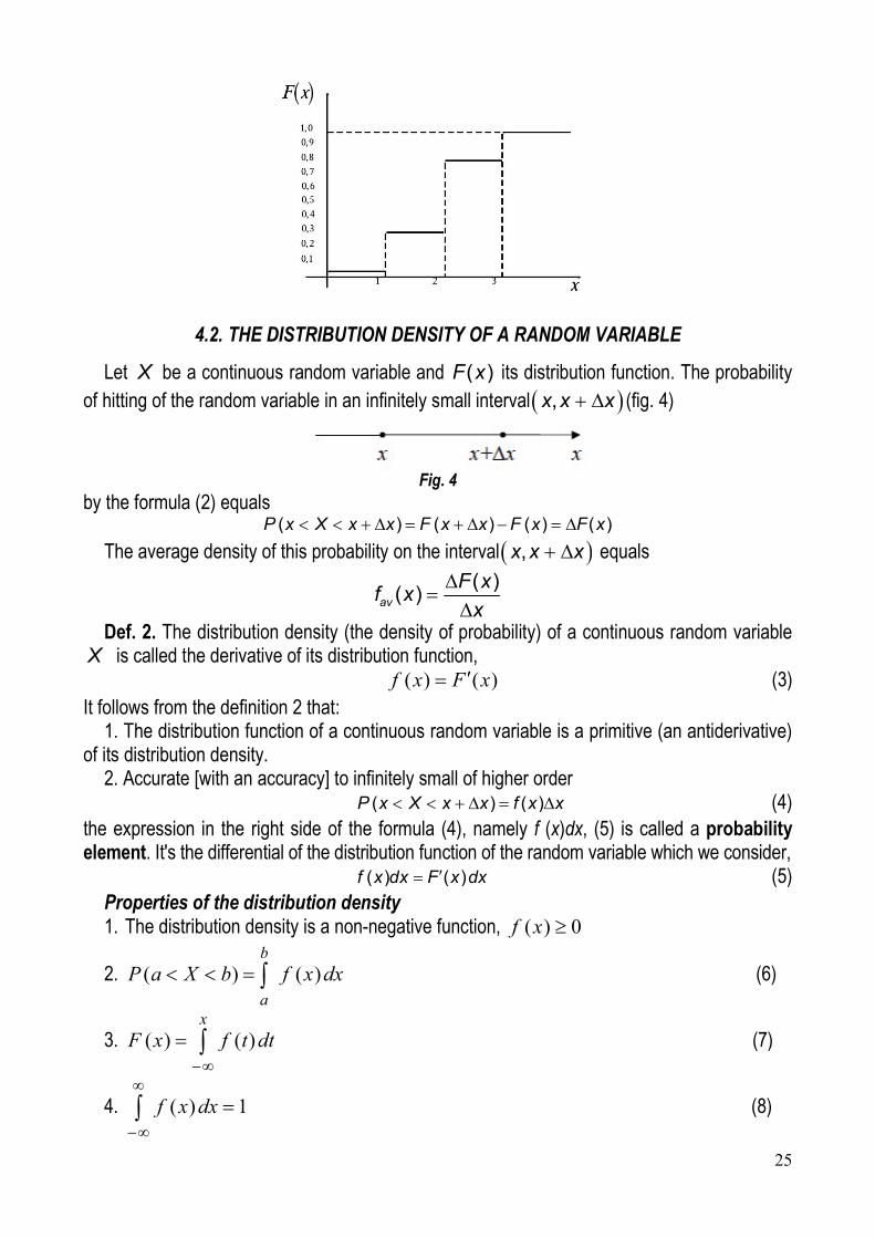
3. )()( 21 xFxF if 21 xx 4. )()()( FFXP (2) Ex.1. From the urn, which contains 3 white and 5 black spheres, 3 spheres are extracted.

Let random variable X be the number of taken out black spheres. Find the distribution law. Plot the graph of function of distribution.

Solution. Possible values of the random variable X are 0, 1, 2, 3. We determine corre-sponding probabilities

1 ( 0)p P X , 2 ( 1)p P X , 3 ( 2)p P X , 4 ( 3)p P X with the help of the classical definition of probability.

33

1 38

1 2 3 1( 0)

8 7 6 56

Cp P X

C

.

1 25 3

2 38

5 3 15( 1)

56 56

C Cp P X

C.

2 15 3

3 38

5 4 3 15 2 30( 2)

2 56 56 56

C Cp P X

C

.

35

4 38

5 4 3 1 10( 3)

2 3 56 56

Cp P X

C.

The distribution law of the random variable X is represented by the next distribution table:

Х 0 1 2 3

Р 56

1

56

15

56

30

56

10

The distribution function of the random variable X , namely of the number of shots which can be done in reality and its graph are given as follows:

If ]1;0(x , then 56

1)0()( XPxF .

If ]2;1(x , then 56

16

56

15

56

1)1()0()( XPXPxF .

If ]3;2(x , then 56

46

56

30

56

16)2(

56

16)( XPxF .

If ];3( x , then 156

10

56

46)3(

56

46)( XPxF .

0, 0,

10,018, 0 1,

5616

( ) 0,286, 1 2,5646

0,821, 2 3,561, 3 .

if x

if x

F x if x

if x

if x

25

4.2. THE DISTRIBUTION DENSITY OF A RANDOM VARIABLE

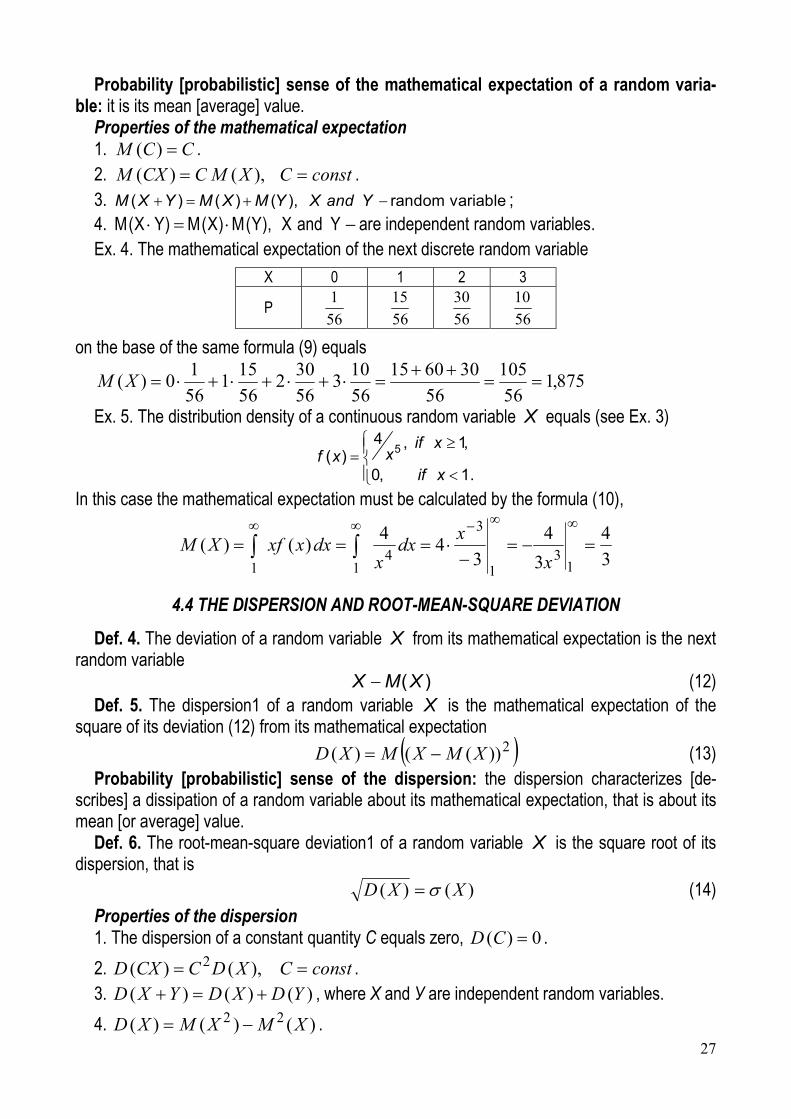
Let X be a continuous random variable and ( )F x its distribution function. The probability of hitting of the random variable in an infinitely small interval ,x x x (fig. 4)

Fig. 4

by the formula (2) equals ( ) ( ) ( ) ( )P x X x x F x x F x F x

The average density of this probability on the interval ,x x x equals

( )( )av

F xf x

x

Def. 2. The distribution density (the density of probability) of a continuous random variable X is called the derivative of its distribution function,

)()( xFxf (3) It follows from the definition 2 that:

1. The distribution function of a continuous random variable is a primitive (an antiderivative) of its distribution density.

2. Accurate [with an accuracy] to infinitely small of higher order ( ) ( )P x X x x f x x (4)

the expression in the right side of the formula (4), namely f (x)dx, (5) is called a probability element. It's the differential of the distribution function of the random variable which we consider,

( ) ( )f x dx F x dx (5) Properties of the distribution density 1. The distribution density is a non-negative function, 0)( xf

2. dxxfbXaPb

a

)()( (6)

3. dttfxFx

)()(

(7)

4. 1)(

dxxf (8)

26

Ex. 2. Let there be given a function xeaxf )( . Find the value of the parameter a so that the function can be the distribution density of some continuous random variable.

Solution. The function in question is a non-negative one. To be the distribution density it must satisfy the condition (8). We find the value of a

1,10

0

dxeadxeadxea xxx

2

1,12)10()01(

0

0

aaaaeaea xx .

Ex. 3. Let there be given a function

54 , 1,

( )0, 1.

if xxf x

if x

.

Find its distribution function. Solution. By virtue of the formula (7) the distribution function of the random variable is

41

41

4

511

11

1

44

4)()(

xt

tdt

tdttfxF

xxxx

4

0, 1,( ) 1

1 , 1.

if xF x

if xx

4.3. THE MATHEMATICAL EXPECTATION OF A RANDOM VARIABLE

Definition of the mathematical expectation Let's suppose that n independent trials on a random variable X are fulfilled and obtained

results are represented by the next table:

X 1x 2x … nx

P 1p 2p … np

According to the statistic definition of probability we introduce the next definition. Def. 3. The mathematical expectation of a discrete random variable X is defined by the

next expression

ii

n

i

pxXM

1

)( (9)

which is the sum of products of its possible values and corresponding probabilities of these values. Let X be a continuous random variable with the distribution density ( )f x . We get the

mathematical expectation of a continuous random variable in the form of the improper integral

dxxfxXM )()(

, if ),( X (10)

dxxfxXMb

a

)()( , if );( baX . (11)

27

Probability [probabilistic] sense of the mathematical expectation of a random varia-ble: it is its mean [average] value.

Properties of the mathematical expectation 1. CCM )( . 2. constCXMCCXM ),()( . 3. ( ) ( ) ( ), random variableM X Y M X M Y X and Y ; 4. M(X Y) M(X) M(Y), X and Y are independent random variables. Ex. 4. The mathematical expectation of the next discrete random variable

Х 0 1 2 3

Р 56

1

56

15

56

30

56

10

on the base of the same formula (9) equals

875,156

105

56

306015

56

103

56

302

56

151

56

10)(

XM

Ex. 5. The distribution density of a continuous random variable X equals (see Ex. 3)

54 , 1,

( )0, 1.

if xxf x

if x

In this case the mathematical expectation must be calculated by the formula (10),

3

4

3

4

34

4)()(

13

1

3

411

x

xdx

xdxxxfXM

4.4 THE DISPERSION AND ROOT-MEAN-SQUARE DEVIATION

Def. 4. The deviation of a random variable X from its mathematical expectation is the next random variable

( )X M X (12) Def. 5. The dispersion1 of a random variable X is the mathematical expectation of the

square of its deviation (12) from its mathematical expectation

2))(()( XMXMXD (13) Probability [probabilistic] sense of the dispersion: the dispersion characterizes [de-

scribes] a dissipation of a random variable about its mathematical expectation, that is about its mean [or average] value.

Def. 6. The root-mean-square deviation1 of a random variable X is the square root of its dispersion, that is

)()( XXD (14)

Properties of the dispersion 1. The dispersion of a constant quantity C equals zero, 0)( CD .

2. constCXDCCXD ),()( 2 . 3. )()()( YDXDYXD , where Х and У are independent random variables.

4. )()()( 22 XMXMXD .

28

Let X be a continuous random variable with the distribution density ( )f x . We get the dis-persion of a continuous random variable in the form of the improper integral

22 2 2( ) ( ( )) ( ) ( ) ( ) ( )D X M X M X x M X f x dx x f x dx M X

(15)

The dispersion of a discrete random variable X is the next expression

2 2 2 2

1

( ) ( ) ( ) ( )n

i i

i

D X M X M X x p M X

(16)

Ex. 6. Calculate the dispersion and root-mean-square deviation of the random variable X of Ex. 4. Solution. The distribution tables of X and its square (see Ex. 4) are

Х 0 1 2 3

Р 56

1

56

15

56

30

56

10

By the formulas (16) and (14) we obtain

018,456

225

56

9012015

56

109

56

304

56

151)( 2

XM .

5024,0875,1018,4)( 2 XD .

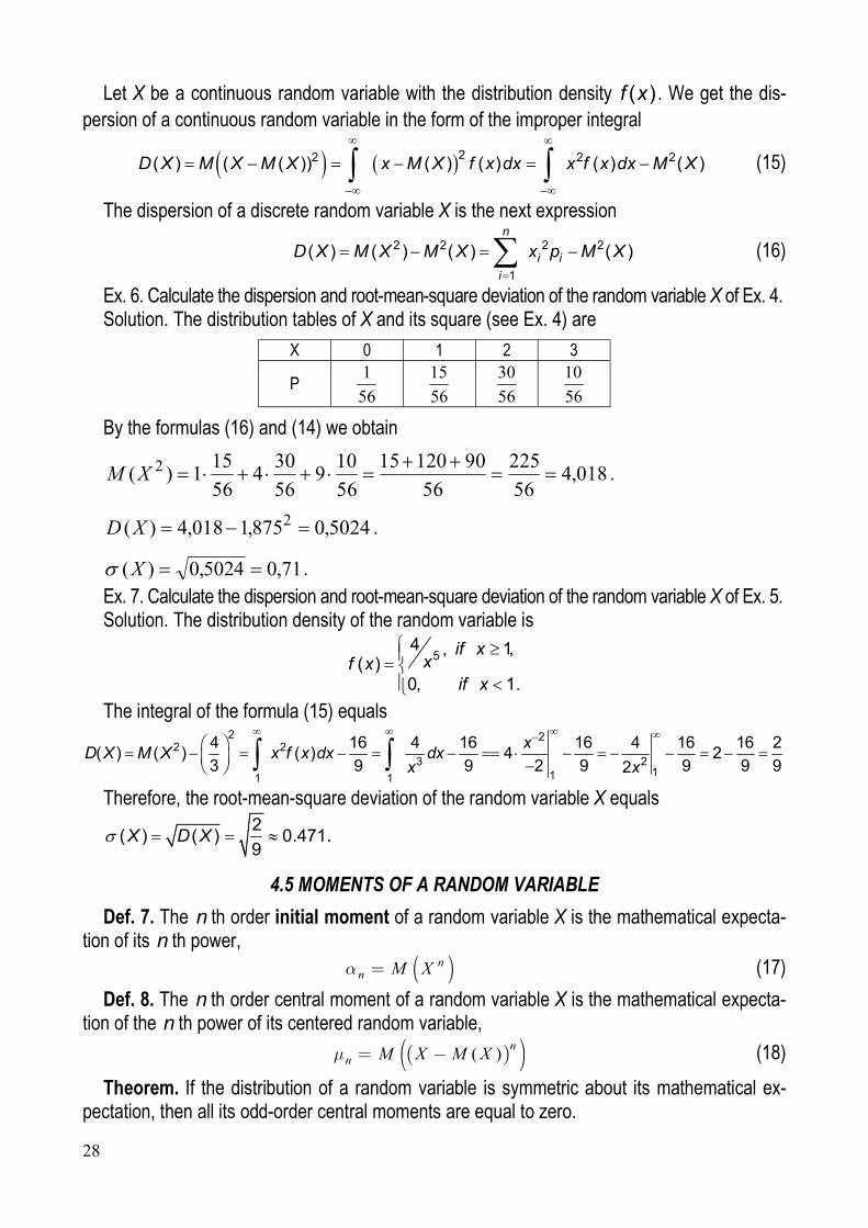
71,05024,0)( X . Ex. 7. Calculate the dispersion and root-mean-square deviation of the random variable X of Ex. 5. Solution. The distribution density of the random variable is

54 , 1,

( )0, 1.

if xxf x

if x

The integral of the formula (15) equals

2 22 2

3 2111 1

4 16 4 16 16 4 16 16 2( ) ( ) ( ) 4 2

3 9 9 2 9 9 9 92

xD X M X x f x dx dx

x x

Therefore, the root-mean-square deviation of the random variable X equals 2

( ) ( ) 0.4719

X D X .

4.5 MOMENTS OF A RANDOM VARIABLE

Def. 7. The n th order initial moment of a random variable X is the mathematical expecta-tion of its n th power,

nn M X (17)

Def. 8. The n th order central moment of a random variable X is the mathematical expecta-tion of the n th power of its centered random variable,

( )n

n M X M X (18)

Theorem. If the distribution of a random variable is symmetric about its mathematical ex-pectation, then all its odd-order central moments are equal to zero.

29

Central moments can be expressed in terms of initial moments, for example those of the second, third and fourth orders are equal

2 22 2 1 1 1 2 12 ,

2 3 33 3 2 1 1 1 1 3 2 1 13 3 3 2 ,

2 3 4 2 44 4 3 1 2 1 1 1 1 4 3 1 2 1 14 6 4 4 6 3 .

There are two quantities which one introduces side by side with the third and fourth central moments of a random variable, namely its asymmetry and excess. The asymmetry of a ran-dom variable X is defined by a quotient

33

À

(19)

and describes the symmetry or non-symmetry of its distribution law. The excess of X is given by a quotient

44

3E

(20)

and describes so-called disnormality of X, that is the deviation of the distribution law of X from the normal distribution (see the next lecture).

Exercise Set 4. Find the distribution law. Plot the graph of function of distribution. Find number characteris-

tics of a random variable. 1. In the lot of 6 components 4 are standard. 2 components are selected at random. Com-

pose the law of distribution of the random variable X, which is the number of standard parts among those selected.

2. Probabilities of hitting the target of the first, second and third shooters are respectively equal to 0,4; 0,3 and 0,6. The random variable X is the number of shots on the target. Find the distribution law of the random variable X .

3. The probability to hitting the target with one shot is equal to 0,6. The random variable X is the number of hitting the target with 5 shots. Find the distribution law of the random variable X; find )(),(),( XXDXM .

Let's suppose that n independent trials on a random variable X are fulfilled, and the ob-tained results are represented by the next tables:

4. Х -2 0 1 5 Р 0,5 0,2 0,1 0,2

5. Х -3 -1 2 4 Р 0,3 0,2 0,4 0,1

6. Х -1 2 3 5 Р 0,1 0,3 0,4 0,2

Build the plotted function of distribution. Find number characteristics of a random variable. Let there be given functions.

7. 0, x 0,

f x A x 2 , 0 x 2,

0, x 2.

8. 0, x 2,

f x A x 2 , 2 x 4,

0, x 4.

30

9. 2

0, x 0,

f x A x , 0 x 2,

0, x 2.

10. 0, x 0,

f x A x, 0 x 1,

0, x 1.

11. 0, x 1,

f x A x 1 , 1 x 2,

0, x 2.

12. 0, x 1,

f x A x 1 , 1 x 2,

0, x 2.

Find the value of the parameter A so that the function can be the distribution density of some continuous random variable. Find its distribution function. Find number characteristics of the random variable. Plot the graph of function of distribution.

5. SOME REMARKABLE DISTRIBUTIONS

5.1. THE UNIFORM DISTRIBUTION

Def. 1. One says that a random variable X has a uniform distribution over an interval ,a b

( X is uniformly distributed or simply X is the uniform distribution over an interval ,a b ) if its distribution density is constant inside and equals zero outside this interval,

, [ ; ],( )

0, [ ; ] .

c if x a bf x

if x a b

(1)

We have to find the value of the constant C, the distribution function and number character-istics of the uniform distribution.

A. Finding the value of C. On the base of property 4 of the distribution density we must have

1( ) 1 ( ) 1

b

a

f x dx cdx cdx c b a cb a

and so the distribution density of the uniform distribution is the next one: 1

, if x [a; b],b af (x)

0, if x [a; b] .

(2)

B. Finding the distribution function of the uniform distribution. Using property 3 of the distribution density, we must study three cases.

0, ,

( ) , ,

1, .

if x a

x aF x if a x b

b aif b x

(3)

C. Finding the number characteristics of the uniform distribution. We’ll limit ourselves to the mathematical expectation, dispersion and root-mean-square de-

viation. For this purpose we’ll make use of the formulas (11), (14), (15).

31

2( )( ) , ( ) , ( ) , ( )

2 12 12

a b b a b a d cM X D X X P c X d

b a (4)

Ex. 1. The time interval of the trolleybus service equals 5 minutes. Find the probability that one will wait a trolleybus no longer then 2 minutes.

Solution. The waiting time T is a random variable uniformly distributed over the inter-val 0,5 , and we have to find the probability 0 2P X

2 00,2 0.4

5 0P

5.2. THE NORMAL DISTRIBUTION

Def. 2. One says that a random variable X has a normal distribution with parameters a , ( 0 ) (or that X is distributed ( , )N a ) if its distribution density is the next function:

2

2( )

21( ; , ) ( )

2

x a

p x a f x e

(5)

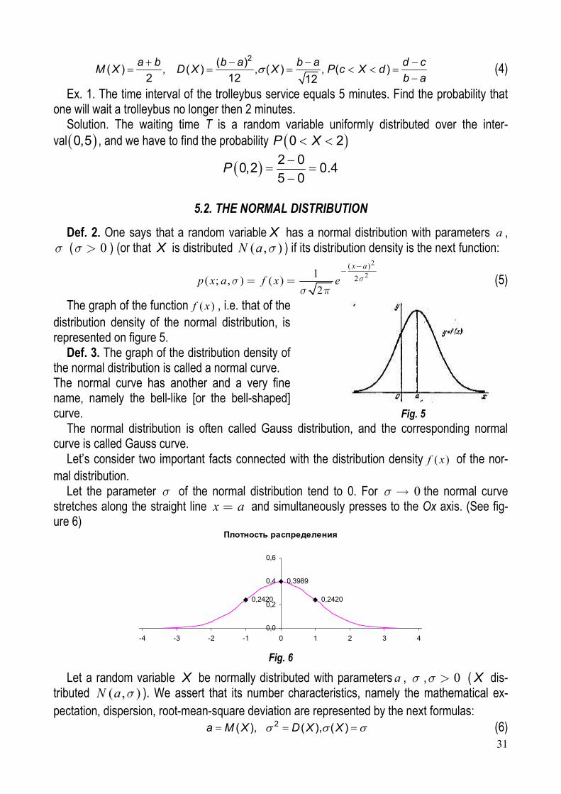
The graph of the function ( )f x , i.e. that of the distribution density of the normal distribution, is represented on figure 5.

Def. 3. The graph of the distribution density of the normal distribution is called a normal curve. The normal curve has another and a very fine name, namely the bell-like [or the bell-shaped] curve. Fig. 5

The normal distribution is often called Gauss distribution, and the corresponding normal curve is called Gauss curve.

Let’s consider two important facts connected with the distribution density ( )f x of the nor-mal distribution.

Let the parameter of the normal distribution tend to 0. For 0 the normal curve stretches along the straight line x a and simultaneously presses to the Ox axis. (See fig-ure 6)

Плотность распределения

0,3989

0,24200,2420

0,0

0,2

0,4

0,6

-4 -3 -2 -1 0 1 2 3 4

Fig. 6

Let a random variable X be normally distributed with parameters a , , 0 ( X dis-tributed ( , )N a ). We assert that its number characteristics, namely the mathematical ex-pectation, dispersion, root-mean-square deviation are represented by the next formulas:

2( ), ( ), ( )a M X D X X (6)

32

Let a random variable X be distributed ( , )N a . The probability of its hitting on an interval ( , ) can be calculated by the next formula:

aaXP )( (7)

where dtex tx

2

0

2

2

1)(

is known as Laplace function.

The probability of the deviation of a random variable X , which is distributed ( , )N a , from its mathematical expectation a is given by the next formula:

2)( aXPXMXP (8)

For example, let 3 . The formula (8) gives 9973,0)3(23 aXP . We’ve got so-called 3σ – rule: with a very large probability 0.9973 all values of the normal

distribution are concentrated in the interval )3;3( aa . Ex.2. A plant makes balls for the bearings. The nominal diameter of the balls is equal to 6

(mm). As a result of an inaccuracy in the production of the balls its actual diameter is a random variable, distributed according to the normal law with an average value of 6 (mm) and mean-square deviation of 0,04 (mm). The balls, whose diameter varies from the nominal by more than 0,1 (mm), are inspected out. Find: 1) what percentage of balls will be rejected on average; 2) probability that the actual diameter of balls will be contained in the range from 5,97 to 6,05 (mm).

Solution. Let the random variable X be an actual diameter of a ball. It is distributed accord-ing to the normal law, i.e. Ν a;σX . If 0a = d = 6 and σ = 0,04 , then Ν 6;0,04X .

Since according to the condition of the task the balls whose diameter differs from the nomi-nal by more than 0,1 (mm) are inspected out, then let us examine the event - 6 > 0,1X . To

find the probability of this event we will use the opposite event - 6 0,1X . Since random variable X is continuous, then

P - 6 0,1 =P - 6 0,1 X X

ε 0,1P - a < ε = 2Φ P - 6 < 0,1 = 2Φ = 2Φ 2,5

σ 0,04X X

Using the table of the values of the function of Laplace, let us find that Φ 2,5 0,4938

P - 6 < 0,1 2 0,4938 = 0,9876 X

If P - 6 < 0,1 +P - 6 > 0,1 =1X X ,

then P - 6 > 0,1 =1-P - 6 < 0,1 =1- 0,9876 = 0,0124X X .

Consequently, 1,24%of the balls will be rejected on average. The probability of its hitting on an interval ( , ) can be calculated by the next formula:

aaXP )(

If Ν 6;0,04X and α = 5,97 , β = 6,05 ,

33

then 6,05 - 6 5,97 - 6P 5,97 < < 6,05 = Φ - Φ = Φ 1,25 +Φ 0,75

0,04 0,04

X

Using the table of the values of the function of Laplace, let us find that Φ 1,25 0,3944 and Φ 0,75 0,2734 .

P 5,97 < < 6,05 0,3944+0,2734 = 0,6678X

5.3. THE EXPONENTIAL DISTRIBUTION

We often deal with a call flow [a flow of calls] in a queuing system. Let’s denote by an in-tensity of the flow, that is the number of calls which take place (on average) per unit of time. Let X be a number of calls during time t. There are many flows (so-called poissonian flows) for which X has Poisson distribution with the parameter a t . In particular, the probability that X will take on a value m equals

( )( ) ( )

!

mt

nt

P X m P m em

Def. 4. Let a random variable X be the time interval between two successive calls of some poissonian call flow. One says that X has the exponential distribution.

Our task is to find the distribution function and density and number characteristics of the ex-ponential distribution.

For positive values of t the events( )X x and 1X coincide. They mean that during time x at least one call will occur. Hence, the distribution function of the random variable X for 0x equals

( ) 1 xF x e (9) The expression 1 xe tends to zero with x , and therefore we can define the distribution

function in question as follows 1 , 0,

( )0, 0.

xe if xF x

if x

(10)

It is continuous for all values of x , and therefore a random variable X which has the expo-nential distribution is a continuous one.

Differentiating the distribution function (10) we’ll obtain the distribution density of the expo-nential distribution,

, 0,( )

0, 0.

xe if xf x

if x

(11)

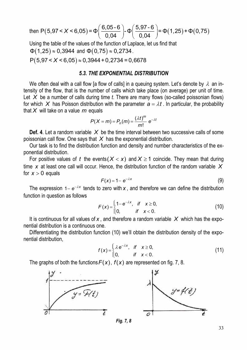
The graphs of both the functions ( )F x , ( )f x are represented on fig. 7, 8.

Fig. 7, 8

34

We assert that its number characteristics, namely the mathematical expectation, dispersion, root-mean-square deviation are represented by the next formulas:

1

)(,1

)(,1

)(,02

XXDXM (12)

The probability of its hitting on an interval ( , )a b can be calculated by the next formula: ba eebXaP )( (13)

Ex.3. Time t of the reliable work of radio-technical system is distributed according to the ex-ponential law. Failure rate of the system is 02,0 . Find the mean time of failure-free opera-tion and the probability of failure-free operation in 80 hours.

Solution. The density of probability distribution of this distribution takes the form 0,020,02 , 0,

( )0, 0.

te if tf t

if t

Mathematical expectation is this mean time of the reliable work of system.

502

100

02,0

11)(

TM (hours).

Let us determine the probability of failure-free operation for 80 hours with the aid of the function of the reliability ( ) (0 )tR t e P X t

2019,0)80( 6,18002,0 eeR .

5.4. BERNOULLI [BINOMIAL] DISTRIBUTION

Def.5. Let a random variable X be the number of successes (the number of occurrences of some event A ) in n independent trials with constant probability of the success A in any trial

( )p P A , ( ) 1P A p q One says that X is distributed binomially (by Bernoulli [binomial] law) or simply: X is Ber-

noulli (binomial) distribution (briefly: X distr. B). Let’s find a probability ( ) ( )nP X m P m , that is the probability of m successes. We’ll get so-called Bernoulli formula:

pqqpCmP mnmmnn 1,)( (14)

The mathematical expectation, dispersion, root-mean-square deviation are represented by the next formulas:

qpnXqpnXDpnXM )(,)(,)( (15) Ex. 4. 6 independently working engines are installed in a shop. Probability for any engine to

work at a given moment is 0.8. Find number characteristics of a random variable X , if the ran-dom variable X is a number of working engines at this moment.

Solution. We can consider setting of an engine as a trial. So we have n = 6 independent tri-als. Let a success A mean that an engine works.

( ) 0.8p P A , ( ) 1 0.2P A p q The random variable X has Bernoulli distribution (briefly “ X distributed B”), it can take on

the values 0,1,2,3,4,5,6, which one calculates by Bernoulli formula (14). For example 0 0 6 6

6 6( 0) (0) 0.2 0.00006P X P C p q

35

1 1 5 56 6( 1) (1) 6 0.8 0.2 0.00154P X P C p q

Using formulas (15), we get ( ) 6 0.8 4.8, ( ) 6 0.8 0.2 0.96,M X n p D X n pq

( ) 0.96 0.979X n pq

5.5. POISSON FORMULA AND DISTRIBUTION

Let a random variable X be distributedB . Let’s suppose that the number n of trials tends to infinity, the probability p of a success A goes to zero, but a product np retains constant,

, 0,n p np const . In this case the limit of the probability ( ) ( )nP X m P m , which is defined by Bernoulli for-

mula (1), equals

em

mPm

n !)( (16)

Def. 6. One says that a discrete random variable X (with non-negative integer possible values) has Poisson distribution with a parameter if its distribution law is given by the next formula (Poisson formula):

( ) ( )!

m

nP X m P m em

(17)

The mathematical expectation, dispersion, root-mean-square deviation are represented by the next formulas:

( ) ( ) , ( )M X D X x (18) Exercise Set 5. Random variable X is normally distributed with the mathematical expectation ( )M X and

the dispersion ( )D X . Find the density of probability distribution )(xf and build the schematic graph of this function. Write down the interval of practically probable values of a random varia-ble. Which is more probable X ; or X ; ?

Exercise ( )M X ( )D X

1 2 4 -1 4 5 6 2 -3 9 -5 -4 -2 -1 3 4 1 0 3 2 5 4 -5 16 -10 -6 0 4 5 3 4 0 5 6 7 6 -2 9 -6 -5 -4 0 7 5 1 0 3 2 6 8 -1 25 -3 1 0 4 9 1 9 -2 2 -1 5 10 -3 4 -4 0 1 6

The mean time of operation of each of the three elements, entering the technical device, is equal to Т hours. For the reliable work of the device the failure-free operation of at least one of these three elements is necessary. Find the probability that the device will work from t1 to t2 hours, if the time of operation of each of the three elements independently is distributed ac-cording to the exponential law.

36

Exercise Т t1 t2 11 800 650 700 12 1000 800 900 13 850 750 820 14 1200 900 1000 15 900 700 900 16 950 720 850

17. The probability of hitting the target with one shot is equal to 0,6. The random variable X is a number of striking the target with 5 shots. Find number characteristics of a random var-iable.

18. Someone expects a telephone call between 19.00 and 20.00. The waiting time of the ring is the random variable X , which has uniform distribution in section [19; 20]. Find probabil-ity that the telephone will ring in the period from 19 hours 22 minutes to 19 hours 46 minutes.

19. Radio equipment for 1000 hours of work goes out of order on the average one time. Find the probability of failure of the radio equipment for 200 hours of work, if the period of fail-ure-free operation is a random variable, distributed according to the exponential law.

20. A basketball player makes three penalty throws. The probability of hit with each throw is equal to 0,7. Find number characteristics of a random variable X , if the random variable X is a number of shots at basket.

6. ELEMENTS OF MATHEMATICAL STATISTICS

6.1. GENERAL REMARKS. SAMPLING METHOD. VARIATION SERIES

Let's suppose that we study some random variable X . We'll dwell upon three typical problems of the mathematical statistics. 1. Exact or approximate determination of the distribution law of a random variable (for ex-

ample it can be stated or hypothesized that a random variable X is distributed normally). 2. Estimation (approximate calculation) of parameters of the distribution law of a random

variable (for example estimation of ;M X ; ( ); ( )X D X As X of a random variable X ). 3. Testing statistical hypotheses (for example testing a hypothesis that a given random vari-

able X is distributed normally). There are various methods of solving such the problems. One of the most widespread is the

sampling method. Suppose that we have some population consisting a great number N of things (the population of the sizeN ) which must be studied with respect to some random vari-able X . We take at random things n N from the population, fulfil their allround testing with respect to X and extend obtained results on the whole population.

On the language of the mathematical statistics we do a sampling of the size n (n N ) getting the sample (of the sizen ) which is subjected to thorough investigation with respect to a random variable in question. A sample must be representative, that is it must certainly repre-sent the population. To be representative the sample must be random one.

A sample of the sizen , which we obtain by a random sampling from the population, we study with the help of so-called variation (or statistical) series. There are variation series of two types namely those discrete and interval.

37

Table 1. A discrete variation series X , ix 1x 2x … kx

im 1m 2m … km

ii

mp

n 1

1

mp

n 2

2

mp

n … k

k

mp

n

1. A discrete variation series contains the row of observed values ix of a random variable X to be the investigated (as the rule in increasing order), the row of numbers im of occur-

rences of these values and the row or their relative frequencies ii

mp

n (table 1).

It must be nmi

k

i

1 and

1

1k

i

i

p

.

Such a discrete variation series can be represented geometrically with the help of a polygon of frequencies or a polygon of relative frequencies. The polygon of relative frequencies is a broken line which joins successively the next points:

1 1 1 2 2 2( , ), ( , ),..., ( , )n n nA x p A x p A x p (see fig. 9).

The polygon of frequencies is a broken line joining successively the other points namely those with ordinates (frequencies) 1 2, ,..., km m m

1 1 1 2 2 2( , ), ( , ),..., ( , )n n nB x p B x p B x p .

If there are a lot of distinct observed values of a random variable X , they can be united in intervals which generate so-called interval variation series.

Fig. 9, 10

2. An interval variation series contains the row of intervals with all observed values of a ran-dom variable X in question, the row of numbers (frequencies) im of hitting of these values in

the i -th interval and the row of corresponding relative frequencies ii

mp

n (table 2).

Table 2. An interval variation series Intervals 10 aa 21 aa … kk aa 1

Frequencies im 1m 2m … km

ii

mp

n 1

1

mp

n 2

2

mp

n k

k

mp

n

38

Just as in the case of a discrete variation series it must be

nmi

k

i

1 and

1

1k

i

i

p

.

The interval variation series can be represented geometrically by a histogram of frequencies or relative frequencies. The histogram of relative frequencies is the set of rectangles with the bases 1( ; ]k ka a , of the lengths 1i i ix a a and the areas i iS p (fig. 10). The altitude of the i -th rectangle of such a histogram equals km h .

The histogram of frequencies contains rectangles of the areas i iS m with the same ba-ses.

Often we form intervals of the same length x (in particular on fig. 10). If one wants to generate k intervals, he can put

k

xxh minmax (1)

where maxx is the greatest and minx is the least of observed values of a random variable X . In practice it's useful sometimes to take instead maxx some greater number and instead minx some less number in the formula (1).

One can preset the length of intervals instead their number. For this purpose he can use the next known approximate formula:

max min

, lg

x x

hn1 3 322

(2)

As the left point of the first interval he can take

min h

a x0 2 (3)

and get then the other points as follows

i ia x h1

(4)

The number k of intervals is determined by the condition

maxka x (5)

which means that the last k -th interval must contain the value maxx of the random varia-ble X in question.

Having an interval variation series we often must compile a corresponding discrete variation series by taking some inner point ix in the ith interval. For example we can take

1

2i i

ia a

x (6)

and obtain the discrete variation series which is given by the table 3. We suppose conditionally that the point ix represents the i-th interval and therefore that the value iX x were ob-

served im times (with the relative frequency ii

mp

n ). It means that the tables 2 and 3 con-

tain the same second and third rows.

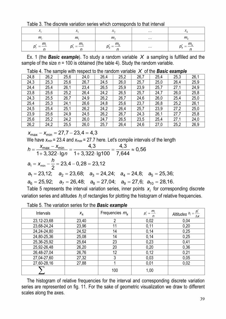
39

Table 3. The discrete variation series which corresponds to that interval ix 1x 2x … kx

im 1m 2m … km

ii

mp

n 1

1

mp

n 2

2

mp

n … k

k

mp

n

Ex. 1 (the Basic example). To study a random variable X a sampling is fulfilled and the sample of the size n = 100 is obtained (the table 4). Study the random variable.

Table 4. The sample with respect to the random variable X of the Basic example 24,8 26,2 25,6 24,0 26,4 25,2 26,7 25,4 25,3 26,1 24,3 25,3 25,6 26,7 24,5 26,0 25,7 25,0 26,4 25,9 24,4 25,4 26,1 23,4 26,5 25,9 23,9 25,7 27,1 24,9 23,8 25,6 25,2 26,4 24,2 26,5 25,7 24,7 26,0 25,8 24,3 25,5 26,7 24,9 26,2 26,7 24,6 26,0 25,4 25,0 25,4 25,3 24,1 26,6 24,8 25,6 23,7 26,8 25,2 26,1 24,5 25,4 25,1 26,2 24,2 26,4 25,7 23,9 27,2 25,0 23,9 25,6 24,9 24,5 26,2 26,7 24,3 26,1 27,7 25,8 25,6 25,2 24,2 26,0 24,7 26,5 23,5 25,4 27,1 24,0 26,2 24,2 25,5 26,0 25,7 26,4 24,6 27,0 25,2 26,9

max min 27,7 23,4 4,3x x We have xmin = 23.4 and xmax = 27.7 here. Let's compile intervals of the length

max min 4,3 4,3

0,561 3,322 lg 1 3,322 lg100 7,644

x xh

n

1 min 23,4 0,28 23,122

ha x

1 2 3 4 5

6 7 8 9 10

23,12; 23,68; 24,24; 24,8; 25,36;

25,92; 26,48; 27,04; 27,6; 28,16.

a a a a a

a a a a a Table 5 represents the interval variation series, inner points ix for corresponding discrete

variation series and altitudes ih of rectangles for plotting the histogram of relative frequencies.

Table 5. The variation series for the Basic example

Intervals kx Frequencies km ii

mp

n Altitudes

ii

ph

x

23,12-23,68 23,40 2 0,02 0,04 23,68-24,24 23,96 11 0,11 0,20 24,24-24,80 24,52 14 0,14 0,25 24,80-25,36 25,08 14 0,14 0,25 25,36-25,92 25,64 23 0,23 0,41 25,92-26,48 26,20 20 0,20 0,36 26,48-27,04 26,76 12 0,12 0,21 27,04-27,60 27,32 3 0,03 0,05 27,60-28,16 27,88 1 0,01 0,02

100 1,00

The histogram of relative frequencies for the interval and corresponding discrete variation series are represented on fig. 11. For the sake of geometric visualization we draw to different scales along the axes.

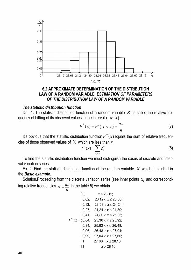
40

Fig. 11

6.2 APPROXIMATE DETERMINATION OF THE DISTRIBUTION LAW OF A RANDOM VARIABLE. ESTIMATION OF PARAMETERS

OF THE DISTRIBUTION LAW OF A RANDOM VARIABLE

The statistic distribution function Def. 1. The statistic distribution function of a random variable X is called the relative fre-

quency of hitting of its observed values in the interval ( , )x ,

n

nxXWxF x )()(* (7)

It's obvious that the statistic distribution function )(* xF equals the sum of relative frequen-cies of those observed values of X which are less than x,

*( )

i

i

x x

F x p

(8)

To find the statistic distribution function we must distinguish the cases of discrete and inter-val variation series.

Ex. 2. Find the statistic distribution function of the random variable X which is studied in the Basic example.

Solution.Proceeding from the discrete variation series (see inner points ix and correspond-

ing relative frequencies ii

mp

n in the table 5) we obtain

*

0, 23,12;

0,02, 23,12 23,68;

0,13, 23,68 24,24;

0,27, 24,24 24,80;

0,41, 24,80 25,36;

( ) 0,64, 25,36 25,92;

0,84, 25,92 26,48;

0,96, 26,48 27,04;

0,99, 27,04 27,60;

1, 27,60 28,16;

1, 28,16.

x

x

x

x

x

F x x

x

x

x

x

x

0,05

k

h

kx

0,20 0,21

0,25

0,36

0,41

23,12 23,68 24,24 24,80 25,36 25,92 26,48 27,04 27,60 0 28,16

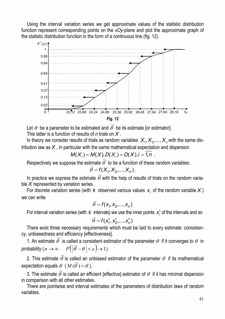
41

Using the interval variation series we get approximate values of the statistic distribution function represent corresponding points on the xOy-plane and plot the approximate graph of the statistic distribution function in the form of a continuous line (fig. 12).

Fig. 12

Let be a parameter to be estimated and ~ be its estimate [or estimator]. This latter is a function of results of n trials on X . In theory we consider results of trials as random variables 1 2, ,..., nX X X with the same dis-

tribution law as X , in particular with the same mathematical expectation and dispersion ( ) ( ), ( ) ( ), 1,i iM X M X D X D X i n .

Respectively we suppose the estimate ~ to be a function of these random variables: 1 2( , ,..., )nf X X X .

In practice we express the estimate ~ with the help of results of trials on the random varia-ble X represented by variation series.

For discrete variation series (with k observed various values ix of the random variable X ) we can write

1 2( , ,..., )nf x x x

For interval variation series (with k intervals) we use the inner points ix of the intervals and so

1 2( , ,..., )nf x x x There exist three necessary requirements which must be laid to every estimate: consisten-

cy, unbiasedness and efficiency [effectiveness]. 1. An estimate ~ is called a consistent estimator of the parameter if it converges to in

probability ( 1~ Pn )

2. This estimate ~ is called an unbiased estimator of the parameter if its mathematical expectation equals ( )

~(M ).

3. The estimate ~ is called an efficient [effective] estimator of if it has minimal dispersion in comparison with all other estimates.

There are pointwise and interval estimates of the parameters of distribution laws of random variables.

0,02

* ( )F x

kx

0,13

0,27

0,41

0,64

0,96

23,12 23,68 24,24 24,80 25,36 25,92 26,48 27,04 27,60 0 28,16

0,84

1

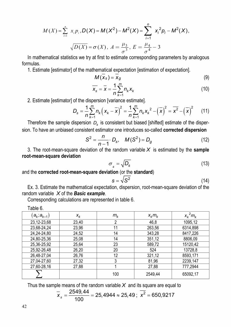
42

ii

n

i

pxXM

1

)( ,

2 2 2 2

1

( ) ( ) ( ) ( )n

i i

i

D X M X M X x p M X ,

)()( XXD , 33

А

, 44

3E

In mathematical statistics we try at first to estimate corresponding parameters by analogous formulas.

1. Estimate [estimator] of the mathematical expectation [estimation of expectation]. ( )s gM x x (9)

1

1 m

s k kk

x x n xn

(10)

2. Estimate [estimator] of the dispersion [variance estimate].

2 2 22 2

1 1

1 1m m

s k k k kk k

D n x x n x x x xn n

(11)

Therefore the sample dispersion sD is consistent but biased [shifted] estimate of the disper-sion. To have an unbiased consistent estimator one introduces so-called corrected dispersion

2 2, ( )1 s g

nS D M S D

n (12)

3. The root-mean-square deviation of the random variable X is estimated by the sample root-mean-square deviation

s sD (13)

and the corrected root-mean-square deviation (or the standard) 2s S (14)

Ex. 3. Estimate the mathematical expectation, dispersion, root-mean-square deviation of the random variable X of the Basic example.

Corresponding calculations are represented in table 6.

Table 6. 1;k ka a kx km k kx m 2

k kx m

23,12-23,68 23,40 2 46,8 1095,12 23,68-24,24 23,96 11 263,56 6314,898 24,24-24,80 24,52 14 343,28 8417,226 24,80-25,36 25,08 14 351,12 8806,09 25,36-25,92 25,64 23 589,72 15120,42 25,92-26,48 26,20 20 524 13728,8 26,48-27,04 26,76 12 321,12 8593,171 27,04-27,60 27,32 3 81,96 2239,147 27,60-28,16 27,88 1 27,88 777,2944

100 2549,44 65092,17

Thus the sample means of the random variable X and its square are equal to 2549,44

25,4944 25,49 ;100sx 2 650,9217x

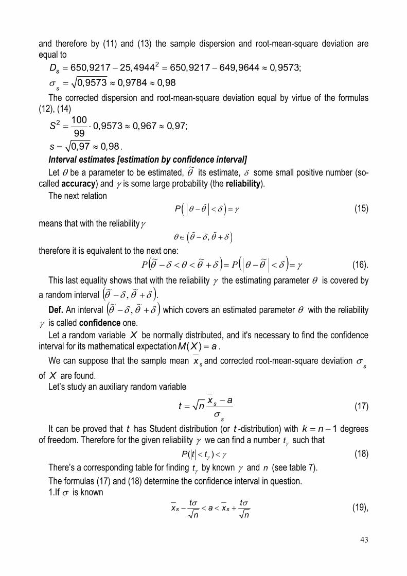
43

and therefore by (11) and (13) the sample dispersion and root-mean-square deviation are equal to

2650,9217 25,4944 650,9217 649,9644 0,9573;sD

0,9573 0,9784 0,98s

The corrected dispersion and root-mean-square deviation equal by virtue of the formulas (12), (14)

2 1000,9573 0,967 0,97;

99S

0,97 0,98s . Interval estimates [estimation by confidence interval] Let be a parameter to be estimated, ~ its estimate, some small positive number (so-

called accuracy) and is some large probability (the reliability). The next relation

P (15)

means that with the reliability

,

therefore it is equivalent to the next one:

~~~PP (16).

This last equality shows that with the reliability the estimating parameter is covered by

a random interval ~,

~.

Def. An interval ~,

~ which covers an estimated parameter with the reliability

is called confidence one. Let a random variable X be normally distributed, and it's necessary to find the confidence

interval for its mathematical expectation ( )M X a .

We can suppose that the sample mean sx and corrected root-mean-square deviation s

of X are found. Let’s study an auxiliary random variable

s

s

x at n

(17)

It can be proved that t has Student distribution (or t -distribution) with 1k n degrees of freedom. Therefore for the given reliability we can find a number t such that

( )P t t (18)

There’s a corresponding table for finding t by known and n (see table 7).

The formulas (17) and (18) determine the confidence interval in question. 1.If is known

s st t

x a xn n

(19),

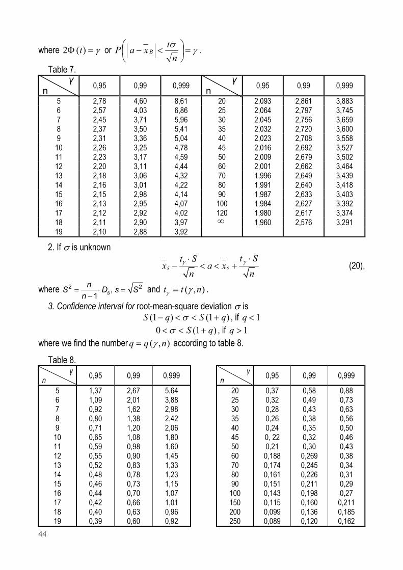
44

where )(2 t or

n

txaP B .

Table 7. γ

n 0,95 0,99 0,999

γ n

0,95 0,99 0,999

5 2,78 4,60 8,61 20 2,093 2,861 3,883 6 2,57 4,03 6,86 25 2,064 2,797 3,745 7 2,45 3,71 5,96 30 2,045 2,756 3,659 8 2,37 3,50 5,41 35 2,032 2,720 3,600 9 2,31 3,36 5,04 40 2,023 2,708 3,558

10 2,26 3,25 4,78 45 2,016 2,692 3,527 11 2,23 3,17 4,59 50 2,009 2,679 3,502 12 2,20 3,11 4,44 60 2,001 2,662 3,464 13 2,18 3,06 4,32 70 1,996 2,649 3,439 14 2,16 3,01 4,22 80 1,991 2,640 3,418 15 2,15 2,98 4,14 90 1,987 2,633 3,403 16 2,13 2,95 4,07 100 1,984 2,627 3,392 17 2,12 2,92 4,02 120 1,980 2,617 3,374 18 2,11 2,90 3,97 1,960 2,576 3,291 19 2,10 2,88 3,92

2. If is unknown

s s

t St Sx a x

n n (20),

where 2 2,1 s

nS D s S

n

and ),( ntt .

3. Confidence interval for root-mean-square deviation is )1()1( qSqS , if 1q

)1(0 qS , if 1q where we find the number ),( nqq according to table 8.

Table 8. γ

n 0,95 0,99 0,999

γ n

0,95 0,99 0,999

5 6 7 8 9

10 11 12 13 14 15 16 17 18 19

1,37 1,09 0,92 0,80 0,71 0,65 0,59 0,55 0,52 0,48 0,46 0,44 0,42 0,40 0,39

2,67 2,01 1,62 1,38 1,20 1,08 0,98 0,90 0,83 0,78 0,73 0,70 0,66 0,63 0,60

5,64 3,88 2,98 2,42 2,06 1,80 1,60 1,45 1,33 1,23 1,15 1,07 1,01 0,96 0,92

20 25 30 35 40 45 50 60 70 80 90

100 150 200 250

0,37 0,32 0,28 0,26 0,24 0, 22 0,21

0,188 0,174 0,161 0,151 0,143 0,115 0,099 0,089

0,58 0,49 0,43 0,38 0,35 0,32 0,30

0,269 0,245 0,226 0,211 0,198 0,160 0,136 0,120

0,88 0,73 0,63 0,56 0,50 0,46 0,43 0,38 0,34 0,31 0,29 0,27

0,211 0,185 0,162

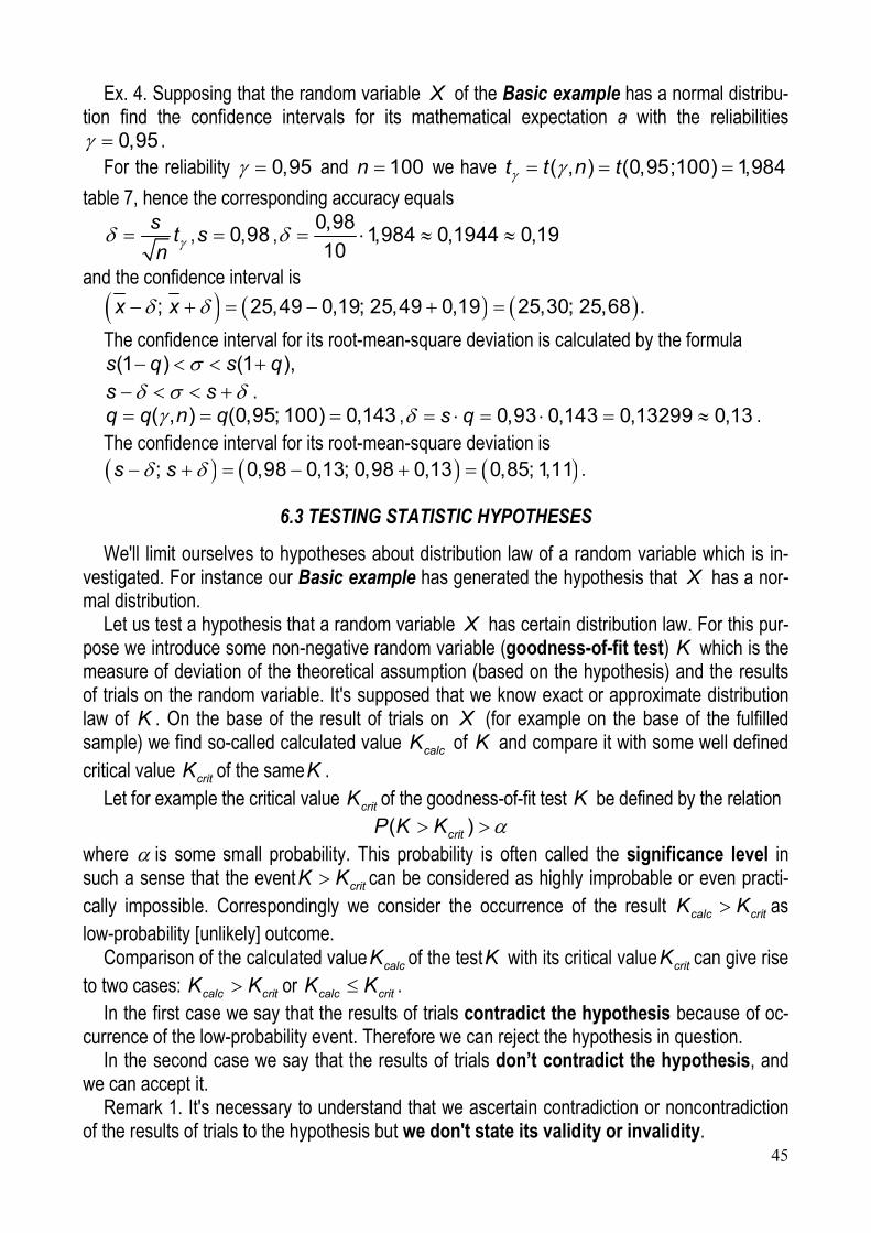
45

Ex. 4. Supposing that the random variable X of the Basic example has a normal distribu-tion find the confidence intervals for its mathematical expectation a with the reliabilities

0,95 . For the reliability 0,95 and 100n we have ( , ) (0,95;100) 1,984t t n t

table 7, hence the corresponding accuracy equals s

tn

, 0,98s ,0,98

1,984 0,1944 0,1910

and the confidence interval is

; 25,49 0,19; 25,49 0,19 25,30; 25,68 .x x

The confidence interval for its root-mean-square deviation is calculated by the formula (1 ) (1 ),s q s q s s .

( , ) (0,95; 100) 0,143q q n q , 0,93 0,143 0,13299 0,13s q . The confidence interval for its root-mean-square deviation is ; 0,98 0,13; 0,98 0,13 0,85; 1,11s s .

6.3 TESTING STATISTIC HYPOTHESES

We'll limit ourselves to hypotheses about distribution law of a random variable which is in-vestigated. For instance our Basic example has generated the hypothesis that X has a nor-mal distribution.

Let us test a hypothesis that a random variable X has certain distribution law. For this pur-pose we introduce some non-negative random variable (goodness-of-fit test) K which is the measure of deviation of the theoretical assumption (based on the hypothesis) and the results of trials on the random variable. It's supposed that we know exact or approximate distribution law of K . On the base of the result of trials on X (for example on the base of the fulfilled sample) we find so-called calculated value calcK of K and compare it with some well defined critical value critK of the sameK .

Let for example the critical value critK of the goodness-of-fit test K be defined by the relation ( )critP K K

where is some small probability. This probability is often called the significance level in such a sense that the event critK K can be considered as highly improbable or even practi-cally impossible. Correspondingly we consider the occurrence of the result calc critK K as low-probability [unlikely] outcome.

Comparison of the calculated value calcK of the testK with its critical value critK can give rise to two cases: calc critK K or calc critK K .

In the first case we say that the results of trials contradict the hypothesis because of oc-currence of the low-probability event. Therefore we can reject the hypothesis in question.

In the second case we say that the results of trials don’t contradict the hypothesis, and we can accept it.

Remark 1. It's necessary to understand that we ascertain contradiction or noncontradiction of the results of trials to the hypothesis but we don't state its validity or invalidity.

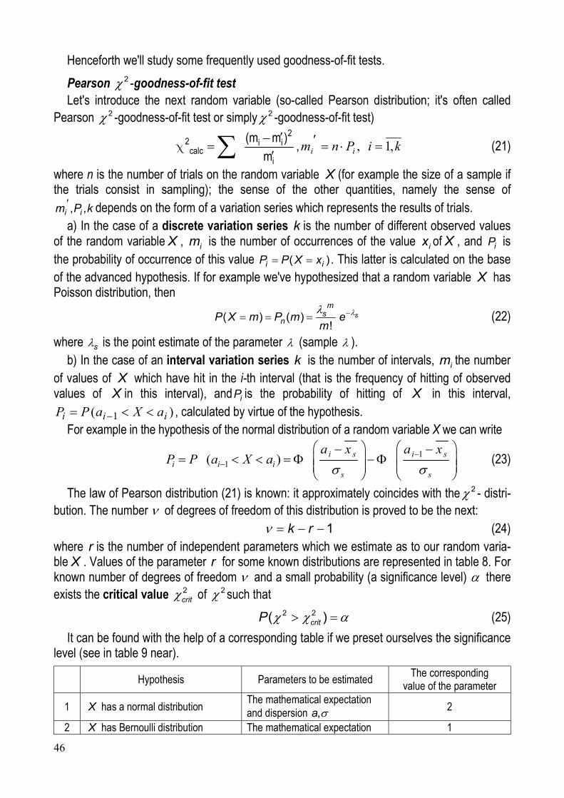
46

Henceforth we'll study some frequently used goodness-of-fit tests.

Pearson 2 -goodness-of-fit test Let's introduce the next random variable (so-called Pearson distribution; it's often called

Pearson 2 -goodness-of-fit test or simply 2 -goodness-of-fit test) 2

2 i icalc

i

(m m )m

, kiPnm ii ,1, (21)

where n is the number of trials on the random variable X (for example the size of a sample if the trials consist in sampling); the sense of the other quantities, namely the sense of

, ,i im P k depends on the form of a variation series which represents the results of trials. a) In the case of a discrete variation series k is the number of different observed values

of the random variable X , im is the number of occurrences of the value ix of X , and iP is the probability of occurrence of this value ( )i iP P X x . This latter is calculated on the base of the advanced hypothesis. If for example we've hypothesized that a random variable X has Poisson distribution, then

( ) ( )!

sm

snP X m P m e

m (22)

where s is the point estimate of the parameter (sample ). b) In the case of an interval variation series k is the number of intervals, im the number

of values of X which have hit in the i-th interval (that is the frequency of hitting of observed values of X in this interval), and iP is the probability of hitting of X in this interval,

)( 1 iii aXaPP , calculated by virtue of the hypothesis. For example in the hypothesis of the normal distribution of a random variable X we can write

11( )

i s i si i i

s s

a x a xP P a X a (23)

The law of Pearson distribution (21) is known: it approximately coincides with the 2 - distri-bution. The number of degrees of freedom of this distribution is proved to be the next:

1k r (24) where r is the number of independent parameters which we estimate as to our random varia-ble X . Values of the parameter r for some known distributions are represented in table 8. For known number of degrees of freedom and a small probability (a significance level) there exists the critical value 2

crit of 2 such that 2 2( )critP (25)

It can be found with the help of a corresponding table if we preset ourselves the significance level (see in table 9 near).

Hypothesis Parameters to be estimated The corresponding

value of the parameter

1 X has a normal distribution The mathematical expectation and dispersion ,a 2

2 X has Bernoulli distribution The mathematical expectation 1

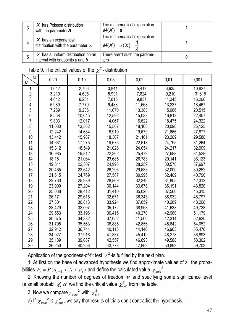
47

3 X has Poisson distribution

with the parametera The mathematical expectation

( )M X a 1

4 X has an exponential

distribution with the parameter

The mathematical expectation

1

( ) ( )M X X 1

5 X has a uniform distribution on an

interval with endpoints a and b There aren't such the parame-ters

0

Table 9. The critical values of the 2 - distribution α

v 0,20 0,10 0,05 0,02 0,01 0,001

1 2 3 4 5 6 7 8 9 10 11 12 13 14 15 16 17 18 19 20 21 22 23 24 25 26 27 28 29 30

1,642 3,219 4,642 5,989 7,289 8,558 9,803

11,030 12,242 13,442 14,631 15,812 16,985 18,151 19,311 20,465 21,615 22,760 23,900 25,038 26,171 27,301 28,429 29,553 30,675 31,795 32,912 34,027 35,139 36,250

2,706 4,605 6,251 7,779 9,236

10,645 12,017 13,362 14,684 15,987 17,275 18,549 19,812 21,064 22,307 23,542 24,769 25,989 27,204 28,412 29,615 30,813 32,007 33,196 34,382 35,563 36,741 37,916 39,087 40,256

3,841 5,991 7,815 9,488

11,070 12,592 14,067 15,507 16,919 18,307 19,675 21,026 22,362 23,685 24,996 26,296 27,587 28,869 30,144 31,410 32,671 33,924 35,172 36,415 37,652 38,885 40,113 41,337 42,557 43,773

5,412 7,824 9,837

11,668 13,388 15,033 16,622 18,168 19,679 21,161 22,618 24,054 25,472 26,783 28,259 29,633 30,995 32,346 33,678 35,020 36,343 37,659 38,968 40,270 41,566 42,856 44,140 45,419 46,693 47,962

6,635 9,210

11,345 13,237 15,086 16,812 18,475 20,090 21,666 23,209 24,795 24,217 27,688 29,141 30,578 32,000 32,409 34,805 36,191 37,566 38,932 40,289 41,638 42,980 42,314 45,642 46,963 48,278 49,588 50,892

10,827 13`,815 16,266 18,467 20,515 22,457 24,322 26,125 27,877 29,588 31,264 32,909 34,528 36,123 37,697 39,252 40,790 42,312 43,820 45,315 46,797 48,268 49,728 51,179 52,620 54,052 55,476 56,893 58,302 59,703

Application of the goodness-of-fit test 2 -is fulfilled by the next plan. 1. At first on the base of advanced hypothesis we find approximate values of all the proba-

bilities )( 1 iii aXaPP and define the calculated value 2calc .

2. Knowing the number of degrees of freedom and specifying some significance level (a small probability) we find the critical value 2

crit from the table.

3. Now we compare 2calc with 2

crit .

a) If 2 2calc crit , we say that results of trials don’t contradict the hypothesis.

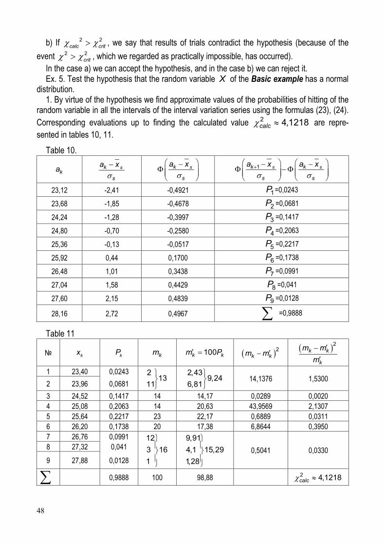
48

b) If 2 2calc crit , we say that results of trials contradict the hypothesis (because of the

event 2 2crit , which we regarded as practically impossible, has occurred).

In the case a) we can accept the hypothesis, and in the case b) we can reject it. Ex. 5. Test the hypothesis that the random variable X of the Basic example has a normal

distribution. 1. By virtue of the hypothesis we find approximate values of the probabilities of hitting of the

random variable in all the intervals of the interval variation series using the formulas (23), (24). Corresponding evaluations up to finding the calculated value 2 4,1218calc are repre-sented in tables 10, 11.

Table 10.

ka sk

s

a x

sk

s

a x

1 s sk k

s s

a x a x

23,12 -2,41 -0,4921 1P =0,0243

23,68 -1,85 -0,4678 2P =0,0681

24,24 -1,28 -0,3997 3P =0,1417

24,80 -0,70 -0,2580 4P =0,2063

25,36 -0,13 -0,0517 5P =0,2217

25,92 0,44 0,1700 6P =0,1738

26,48 1,01 0,3438 7P =0,0991

27,04 1,58 0,4429 8P =0,041

27,60 2,15 0,4839 9P =0,0128

28,16 2,72 0,4967 =0,9888

Table 11

№ kx kP km 100k km P 2k km m

2k k

k

m m

m

1 23,40 0,0243

213

11

2,439,24

6,81 14,1376 1,5300

2 23,96 0,0681

3 24,52 0,1417 14 14,17 0,0289 0,0020 4 25,08 0,2063 14 20,63 43,9569 2,1307 5 25,64 0,2217 23 22,17 0,6889 0,0311 6 26,20 0,1738 20 17,38 6,8644 0,3950 7 26,76 0,0991

12

3 16

1

9,91

4,1 15,29

1,28

0,5041 0,0330 8 27,32 0,041

9 27,88 0,0128

0,9888 100 98,88 2 4,1218calc

49

2. Let's choose the significance level (a small probability) 0,05 . Finding by the formula (25) the number of degrees of freedom

1k r , 6k , 2r , 3 we find the critical value 2 2( , ) (3, 0,05) 7,815crit crit from table 9.

3. We've obtained 2 24,1218calc crit . It means that the results of trials on the random variable X in question don’t contradict the hypothesis that its distribution law is a normal one.

Kolmogorov goodness-of-fit test Let X be a continuous random variable, and we advance the next hypothesis: the given

function ( )F X is the distribution function of this random variable. Let a number D be the greatest value of the absolute value of a difference of the func-

tion ( )F X and statistical distribution function ( )F X that is *

.1max ( ) ( )calc i i

i kD n F x F x

(26)

Table 12 gives some values of the critD .

Table 12. The values of the critD . α 0,20 0,10 0,05 0,02 0,01 0,001

critD 1,073 1,224 1,358 1,520 1,627 1,950

a) If calc critD D , we say that results of trials don’t contradict the hypothesis. b) If calc critD D , we say that results of trials contradict the hypothesis (because of the

event calc critD D , which we regarded as practically impossible, has occurred). In the case a) we can accept the hypothesis, and in the case b) we can reject it.

Tasks for individual work on mathematical statistics

PROBLEM. 100 independent trials are fulfilled on a random variable X , and the results of trials are represented by corresponding sample of the size n = 100.

1. Compile the interval variation series for the random variable X , plot the histogram of relative frequencies and approximate graph of the distribution density. Find the statistical distribution function for the interval variation series and construct its approximate graph.

2. On the base of the interval variation series form the discreet variation series by taking inner points in each interval. Construct the polygon of relative frequencies. Form the statis-tical distribution function for the discreet variation series and plot its graph.

3. Calculate the sample mean [the sample average], dispersion, root-mean-square devia-tion of the random variable. Draw a conclusion as to symmetry of its distribution law and devia-tion of this law from the normal distribution.

4. Find the corrected dispersion and root-mean-square deviation of the random variable. Compare their values with corresponding sample estimators.

5. Search out the confidence intervals for the mathematical expectation of the random vari-able X with reliabilities 0.95 and 0.99, basing on the hypothesis of its normal distribution.

6. Find approximate values of the probabilities of hitting of the random variable X on all the intervals of its variation series proceeding from the hypothesis of the normal distribution of X .

7. Test the hypothesis on the normal distribution of the random variable X with the signifi-cance levels 0.01,0.025,0.05 making use of Pearson 2 -goodness-of-fit tests.

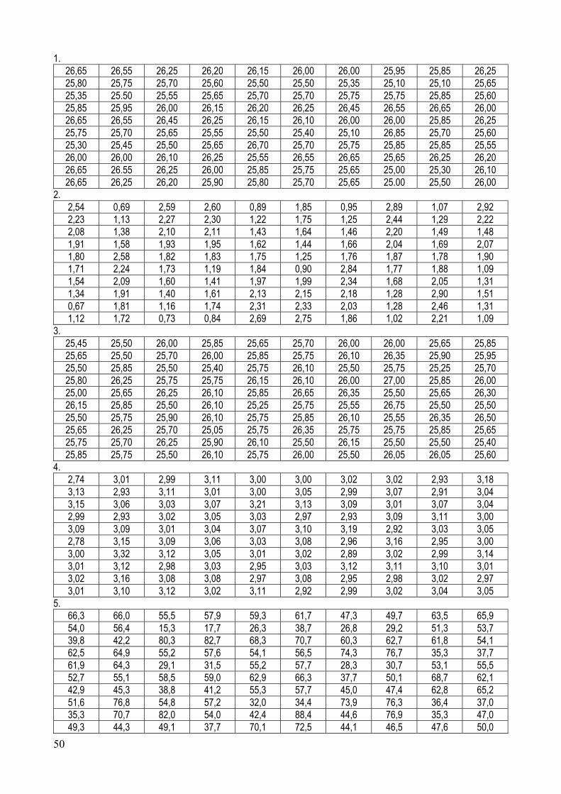
50

1. 26,65 26,55 26,25 26,20 26,15 26,00 26,00 25,95 25,85 26,25 25,80 25,75 25,70 25,60 25,50 25,50 25,35 25,10 25,10 25,65 25,35 25.50 25,55 25,65 25,70 25,70 25,75 25,75 25,85 25,60 25,85 25,95 26,00 26,15 26,20 26,25 26,45 26,55 26,65 26,00 26,65 26,55 26,45 26,25 26,15 26,10 26,00 26,00 25,85 26,25 25,75 25,70 25,65 25,55 25,50 25,40 25,10 26,85 25,70 25,60 25,30 25,45 25,50 25,65 26,70 25,70 25,75 25,85 25,85 25,55 26,00 26,00 26,10 26,25 25,55 26,55 26,65 25,65 26,25 26,20 26,65 26.55 26,25 26,00 25,85 25,75 25,65 25,00 25,30 26,10 26,65 26,25 26,20 25,90 25,80 25,70 25,65 25.00 25,50 26,00

2. 2,54 0,69 2,59 2,60 0,89 1,85 0,95 2,89 1,07 2,92 2,23 1,13 2,27 2,30 1,22 1,75 1,25 2,44 1,29 2,22 2,08 1,38 2,10 2,11 1,43 1,64 1,46 2,20 1,49 1,48 1,91 1,58 1,93 1,95 1,62 1,44 1,66 2,04 1,69 2,07 1,80 2,58 1,82 1,83 1,75 1,25 1,76 1,87 1,78 1,90 1,71 2,24 1,73 1,19 1,84 0,90 2,84 1,77 1,88 1,09 1,54 2,09 1,60 1,41 1,97 1,99 2,34 1,68 2,05 1,31 1,34 1,91 1,40 1,61 2,13 2,15 2,18 1,28 2,90 1,51 0,67 1,81 1,16 1,74 2,31 2,33 2,03 1,28 2,46 1,31 1,12 1,72 0,73 0,84 2,69 2,75 1,86 1,02 2,21 1,09

3. 25,45 25,50 26,00 25,85 25,65 25,70 26,00 26,00 25,65 25,85 25,65 25,50 25,70 26,00 25,85 25,75 26,10 26,35 25,90 25,95 25,50 25,85 25,50 25,40 25,75 26,10 25,50 25,75 25,25 25,70 25,80 26,25 25,75 25,75 26,15 26,10 26,00 27,00 25,85 26,00 25,00 25,65 26,25 26,10 25,85 26,65 26,35 25,50 25,65 26,30 26,15 25,85 25,50 26,10 25,25 25,75 25,55 26,75 25,50 25,50 25,50 25,75 25,90 26,10 25,75 25,85 26,10 25,55 26,35 26,50 25,65 26,25 25,70 25,05 25,75 26,35 25,75 25,75 25,85 25,65 25,75 25,70 26,25 25,90 26,10 25,50 26,15 25,50 25,50 25,40 25,85 25,75 25,50 26,10 25,75 26,00 25,50 26,05 26,05 25,60

4. 2,74 3,01 2,99 3,11 3,00 3,00 3,02 3,02 2,93 3,18 3,13 2,93 3,11 3,01 3,00 3,05 2,99 3,07 2,91 3,04 3,15 3,06 3,03 3,07 3,21 3,13 3,09 3,01 3,07 3,04 2,99 2,93 3,02 3,05 3,03 2,97 2,93 3,09 3,11 3,00 3,09 3,09 3,01 3,04 3,07 3,10 3,19 2,92 3,03 3,05 2,78 3,15 3,09 3,06 3,03 3,08 2,96 3,16 2,95 3,00 3,00 3,32 3,12 3,05 3,01 3,02 2,89 3,02 2,99 3,14 3,01 3,12 2,98 3,03 2,95 3,03 3,12 3,11 3,10 3,01 3,02 3,16 3,08 3,08 2,97 3,08 2,95 2,98 3,02 2,97 3,01 3,10 3,12 3,02 3,11 2,92 2,99 3,02 3,04 3,05

5. 66,3 66,0 55,5 57,9 59,3 61,7 47,3 49,7 63,5 65,9 54,0 56,4 15,3 17,7 26,3 38,7 26,8 29,2 51,3 53,7 39,8 42,2 80,3 82,7 68,3 70,7 60,3 62,7 61,8 54,1 62,5 64,9 55,2 57,6 54,1 56,5 74,3 76,7 35,3 37,7 61,9 64,3 29,1 31,5 55,2 57,7 28,3 30,7 53,1 55,5 52,7 55,1 58,5 59,0 62,9 66,3 37,7 50,1 68,7 62,1 42,9 45,3 38,8 41,2 55,3 57,7 45,0 47,4 62,8 65,2 51,6 76,8 54,8 57,2 32,0 34,4 73,9 76,3 36,4 37,0 35,3 70,7 82,0 54,0 42,4 88,4 44,6 76,9 35,3 47,0 49,3 44,3 49,1 37,7 70,1 72,5 44,1 46,5 47,6 50,0

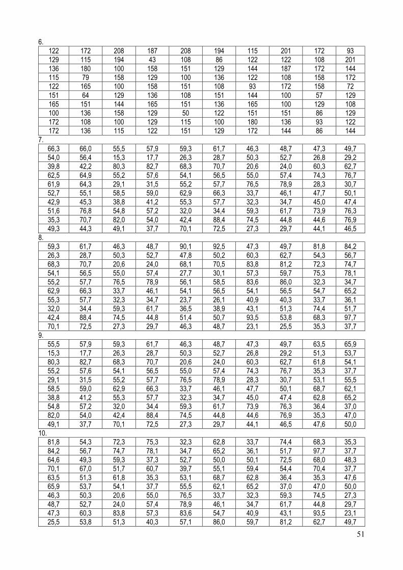
51

6. 122 172 208 187 208 194 115 201 172 93 129 115 194 43 108 86 122 122 108 201 136 180 100 158 151 129 144 187 172 144 115 79 158 129 100 136 122 108 158 172 122 165 100 158 151 108 93 172 158 72 151 64 129 136 108 151 144 100 57 129 165 151 144 165 151 136 165 100 129 108 100 136 158 129 50 122 151 151 86 129 172 108 100 129 115 100 180 136 93 122 172 136 115 122 151 129 172 144 86 144

7. 66,3 66,0 55,5 57,9 59,3 61,7 46,3 48,7 47,3 49,7 54,0 56,4 15,3 17,7 26,3 28,7 50,3 52,7 26,8 29,2 39,8 42,2 80,3 82,7 68,3 70,7 20,6 24,0 60,3 62,7 62,5 64,9 55,2 57,6 54,1 56,5 55,0 57,4 74,3 76,7 61,9 64,3 29,1 31,5 55,2 57,7 76,5 78,9 28,3 30,7 52,7 55,1 58,5 59,0 62,9 66,3 33,7 46,1 47,7 50,1 42,9 45,3 38,8 41,2 55,3 57,7 32,3 34,7 45,0 47,4 51,6 76,8 54,8 57,2 32,0 34,4 59,3 61,7 73,9 76,3 35,3 70,7 82,0 54,0 42,4 88,4 74,5 44,8 44,6 76,9 49,3 44,3 49,1 37,7 70,1 72,5 27,3 29,7 44,1 46,5

8. 59,3 61,7 46,3 48,7 90,1 92,5 47,3 49,7 81,8 84,2 26,3 28,7 50,3 52,7 47,8 50,2 60,3 62,7 54,3 56,7 68,3 70,7 20,6 24,0 68,1 70,5 83,8 81,2 72,3 74,7 54,1 56,5 55,0 57,4 27,7 30,1 57,3 59,7 75,3 78,1 55,2 57,7 76,5 78,9 56,1 58,5 83,6 86,0 32,3 34,7 62,9 66,3 33,7 46,1 54,1 56,5 54,1 56,5 54,7 65,2 55,3 57,7 32,3 34,7 23,7 26,1 40,9 40,3 33,7 36,1 32,0 34,4 59,3 61,7 36,5 38,9 43,1 51,3 74,4 51,7 42,4 88,4 74,5 44,8 51,4 50,7 93,5 53,8 68,3 97,7 70,1 72,5 27,3 29,7 46,3 48,7 23,1 25,5 35,3 37,7

9. 55,5 57,9 59,3 61,7 46,3 48,7 47,3 49,7 63,5 65,9 15,3 17,7 26,3 28,7 50,3 52,7 26,8 29,2 51,3 53,7 80,3 82,7 68,3 70,7 20,6 24,0 60,3 62,7 61,8 54,1 55,2 57,6 54,1 56,5 55,0 57,4 74,3 76,7 35,3 37,7 29,1 31,5 55,2 57,7 76,5 78,9 28,3 30,7 53,1 55,5 58,5 59,0 62,9 66,3 33,7 46,1 47,7 50,1 68,7 62,1 38,8 41,2 55,3 57,7 32,3 34,7 45,0 47,4 62,8 65,2 54,8 57,2 32,0 34,4 59,3 61,7 73,9 76,3 36,4 37,0 82,0 54,0 42,4 88,4 74,5 44,8 44,6 76,9 35,3 47,0 49,1 37,7 70,1 72,5 27,3 29,7 44,1 46,5 47,6 50,0

10. 81,8 54,3 72,3 75,3 32,3 62,8 33,7 74,4 68,3 35,3 84,2 56,7 74,7 78,1 34,7 65,2 36,1 51,7 97,7 37,7 64,6 49,3 59,3 37,3 52,7 50,0 50,1 72,5 68,0 48,3 70,1 67,0 51,7 60,7 39,7 55,1 59,4 54,4 70,4 37,7 63,5 51,3 61,8 35,3 53,1 68,7 62,8 36,4 35,3 47,6 65,9 53,7 54,1 37,7 55,5 62,1 65,2 37,0 47,0 50,0 46,3 50,3 20,6 55,0 76,5 33,7 32,3 59,3 74,5 27,3 48,7 52,7 24,0 57,4 78,9 46,1 34,7 61,7 44,8 29,7 47,3 60,3 83,8 57,3 83,6 54,7 40,9 43,1 93,5 23,1 25,5 53,8 51,3 40,3 57,1 86,0 59,7 81,2 62,7 49,7

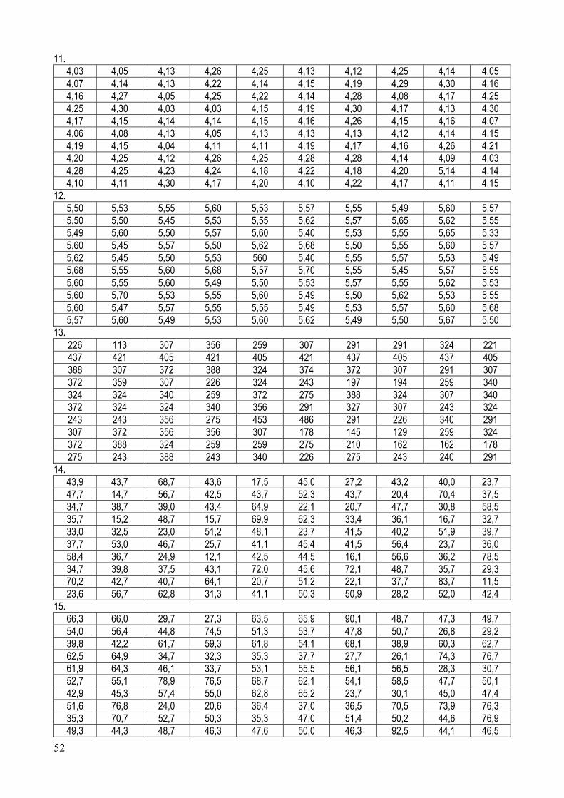
52

11. 4,03 4,05 4,13 4,26 4,25 4,13 4,12 4,25 4,14 4,05 4,07 4,14 4,13 4,22 4,14 4,15 4,19 4,29 4,30 4,16 4,16 4,27 4,05 4,25 4,22 4,14 4,28 4,08 4,17 4,25 4,25 4,30 4,03 4,03 4,15 4,19 4,30 4,17 4,13 4,30 4,17 4,15 4,14 4,14 4,15 4,16 4,26 4,15 4,16 4,07 4,06 4,08 4,13 4,05 4,13 4,13 4,13 4,12 4,14 4,15 4,19 4,15 4,04 4,11 4,11 4,19 4,17 4,16 4,26 4,21 4,20 4,25 4,12 4,26 4,25 4,28 4,28 4,14 4,09 4,03 4,28 4,25 4,23 4,24 4,18 4,22 4,18 4,20 5,14 4,14 4,10 4,11 4,30 4,17 4,20 4,10 4,22 4,17 4,11 4,15

12. 5,50 5,53 5,55 5,60 5,53 5,57 5,55 5,49 5,60 5,57 5,50 5,50 5,45 5,53 5,55 5,62 5,57 5,65 5,62 5,55 5,49 5,60 5,50 5,57 5,60 5,40 5,53 5,55 5,65 5,33 5,60 5,45 5,57 5,50 5,62 5,68 5,50 5,55 5,60 5,57 5,62 5,45 5,50 5,53 560 5,40 5,55 5,57 5,53 5,49 5,68 5,55 5,60 5,68 5,57 5,70 5,55 5,45 5,57 5,55 5,60 5,55 5,60 5,49 5,50 5,53 5,57 5,55 5,62 5,53 5,60 5,70 5,53 5,55 5,60 5,49 5,50 5,62 5,53 5,55 5,60 5,47 5,57 5,55 5,55 5,49 5,53 5,57 5,60 5,68 5,57 5,60 5,49 5,53 5,60 5,62 5,49 5,50 5,67 5,50

13. 226 113 307 356 259 307 291 291 324 221 437 421 405 421 405 421 437 405 437 405 388 307 372 388 324 374 372 307 291 307 372 359 307 226 324 243 197 194 259 340 324 324 340 259 372 275 388 324 307 340 372 324 324 340 356 291 327 307 243 324 243 243 356 275 453 486 291 226 340 291 307 372 356 356 307 178 145 129 259 324 372 388 324 259 259 275 210 162 162 178 275 243 388 243 340 226 275 243 240 291

14. 43,9 43,7 68,7 43,6 17,5 45,0 27,2 43,2 40,0 23,7 47,7 14,7 56,7 42,5 43,7 52,3 43,7 20,4 70,4 37,5 34,7 38,7 39,0 43,4 64,9 22,1 20,7 47,7 30,8 58,5 35,7 15,2 48,7 15,7 69,9 62,3 33,4 36,1 16,7 32,7 33,0 32,5 23,0 51,2 48,1 23,7 41,5 40,2 51,9 39,7 37,7 53,0 46,7 25,7 41,1 45,4 41,5 56,4 23,7 36,0 58,4 36,7 24,9 12,1 42,5 44,5 16,1 56,6 36,2 78,5 34,7 39,8 37,5 43,1 72,0 45,6 72,1 48,7 35,7 29,3 70,2 42,7 40,7 64,1 20,7 51,2 22,1 37,7 83,7 11,5 23,6 56,7 62,8 31,3 41,1 50,3 50,9 28,2 52,0 42,4

15. 66,3 66,0 29,7 27,3 63,5 65,9 90,1 48,7 47,3 49,7 54,0 56,4 44,8 74,5 51,3 53,7 47,8 50,7 26,8 29,2 39,8 42,2 61,7 59,3 61,8 54,1 68,1 38,9 60,3 62,7 62,5 64,9 34,7 32,3 35,3 37,7 27,7 26,1 74,3 76,7 61,9 64,3 46,1 33,7 53,1 55,5 56,1 56,5 28,3 30,7 52,7 55,1 78,9 76,5 68,7 62,1 54,1 58,5 47,7 50,1 42,9 45,3 57,4 55,0 62,8 65,2 23,7 30,1 45,0 47,4 51,6 76,8 24,0 20,6 36,4 37,0 36,5 70,5 73,9 76,3 35,3 70,7 52,7 50,3 35,3 47,0 51,4 50,2 44,6 76,9 49,3 44,3 48,7 46,3 47,6 50,0 46,3 92,5 44,1 46,5

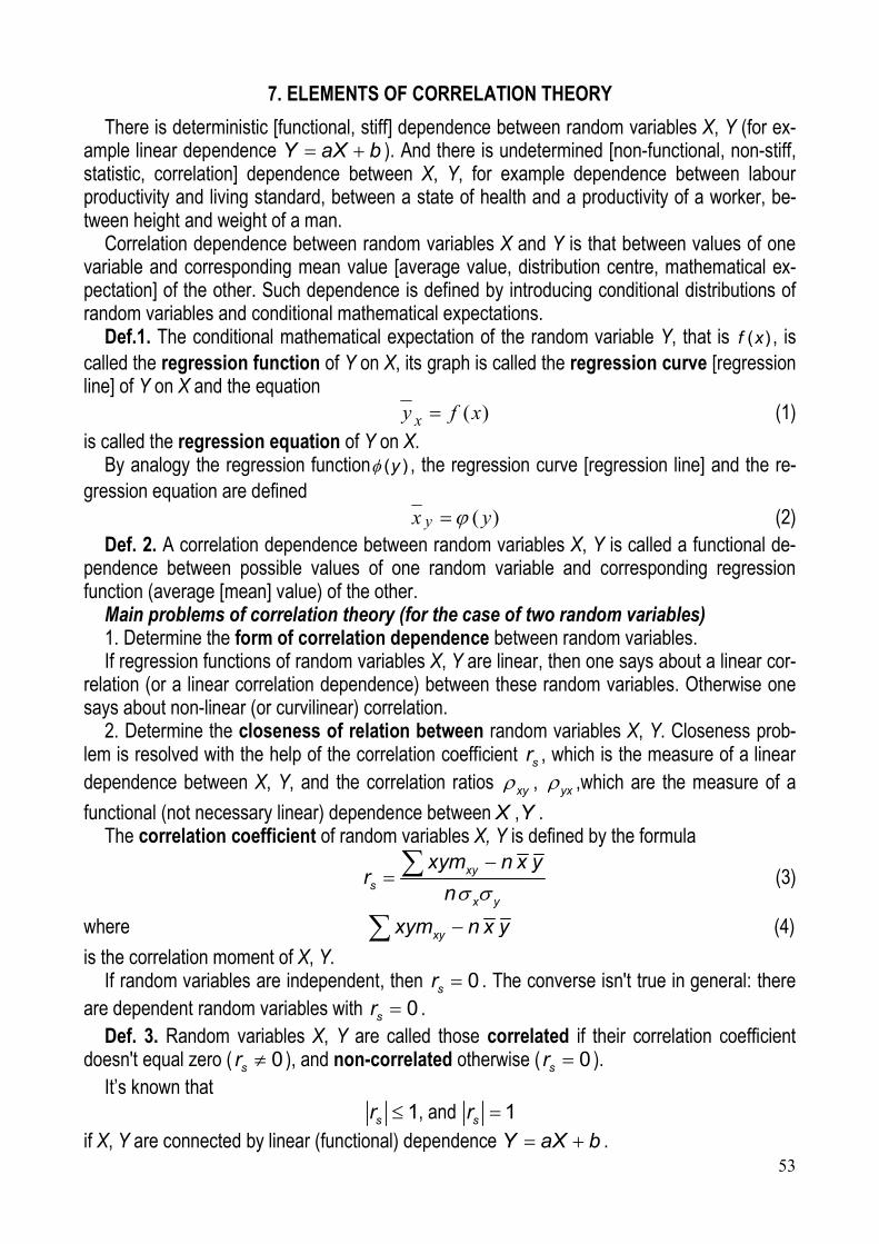
53

7. ELEMENTS OF CORRELATION THEORY

There is deterministic [functional, stiff] dependence between random variables X, Y (for ex-ample linear dependence Y aX b ). And there is undetermined [non-functional, non-stiff, statistic, correlation] dependence between X, Y, for example dependence between labour productivity and living standard, between a state of health and a productivity of a worker, be-tween height and weight of a man.

Correlation dependence between random variables X and Y is that between values of one variable and corresponding mean value [average value, distribution centre, mathematical ex-pectation] of the other. Such dependence is defined by introducing conditional distributions of random variables and conditional mathematical expectations.

Def.1. The conditional mathematical expectation of the random variable Y, that is ( )f x , is called the regression function of Y on X, its graph is called the regression curve [regression line] of Y on X and the equation

)(xfy x (1) is called the regression equation of Y on X.

By analogy the regression function ( )y , the regression curve [regression line] and the re-gression equation are defined

)( yx y (2) Def. 2. A correlation dependence between random variables X, Y is called a functional de-

pendence between possible values of one random variable and corresponding regression function (average [mean] value) of the other.

Main problems of correlation theory (for the case of two random variables) 1. Determine the form of correlation dependence between random variables. If regression functions of random variables X, Y are linear, then one says about a linear cor-

relation (or a linear correlation dependence) between these random variables. Otherwise one says about non-linear (or curvilinear) correlation.

2. Determine the closeness of relation between random variables X, Y. Closeness prob-lem is resolved with the help of the correlation coefficient sr , which is the measure of a linear dependence between X, Y, and the correlation ratios xy , yx ,which are the measure of a

functional (not necessary linear) dependence between X ,Y . The correlation coefficient of random variables X, Y is defined by the formula

xys

x y

xym n x yr

n

(3)

where xyxym n x y (4)

is the correlation moment of X, Y. If random variables are independent, then 0sr . The converse isn't true in general: there

are dependent random variables with 0sr . Def. 3. Random variables X, Y are called those correlated if their correlation coefficient

doesn't equal zero ( 0sr ), and non-correlated otherwise ( 0sr ). It’s known that

1sr , and 1sr if X, Y are connected by linear (functional) dependence Y aX b .

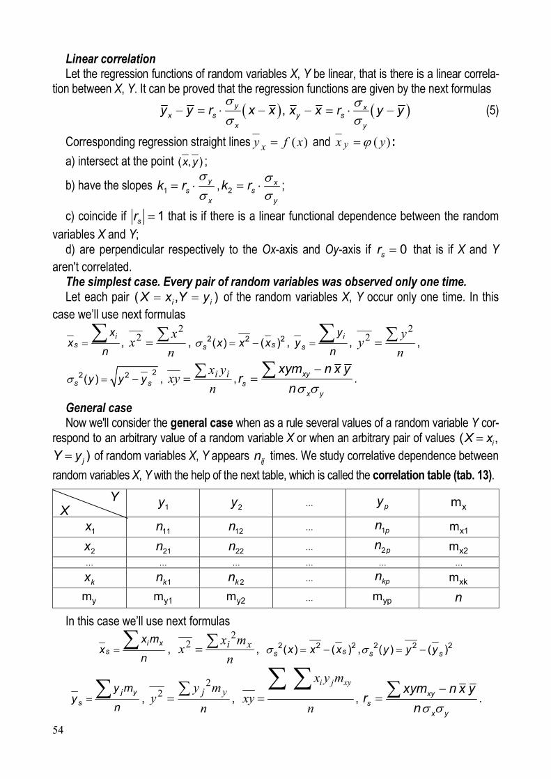
54

Linear correlation Let the regression functions of random variables X, Y be linear, that is there is a linear correla-

tion between X, Y. It can be proved that the regression functions are given by the next formulas

,yx s

x

y y r x x

xy s

y

x x r y y

(5)

Corresponding regression straight lines )(xfy x and )( yx y :

a) intersect at the point ( , )x y ;

b) have the slopes 1y

sx

k r

, 2x

sy

k r

;

c) coincide if 1sr that is if there is a linear functional dependence between the random variables X and Y;

d) are perpendicular respectively to the Ox-axis and Oy-axis if 0sr that is if X and Y aren't correlated.

The simplest case. Every pair of random variables was observed only one time. Let each pair ( , )i iX x Y y of the random variables X, Y occur only one time. In this

case we’ll use next formulas

is

xx

n ,

n

xx

22 , 2 2 2( ) ( )ss x x x ,

is

yy

n ,

n

yy

22 ,

22 2( )s sy y y , n

yxxy ii , xy

sx y

xym n x yr

n

.

General case Now we'll consider the general case when as a rule several values of a random variable Y cor-

respond to an arbitrary value of a random variable X or when an arbitrary pair of values ( ,iX x )jY y of random variables X, Y appears ijn times. We study correlative dependence between

random variables X, Y with the help of the next table, which is called the correlation table (tab. 13).

Y

X 1y 2y … py xm

1x 11n 12n … 1pn x1m

2x 21n 22n … 2pn x2m

… … … … … …

kx 1kn 2kn … kpn xkm

ym y1m y2m … ypm n

In this case we’ll use next formulas

i xs

x mx

n ,

n

mxx xi

22 , 2 2 2( ) ( )ss x x x , 2 2 2( ) ( )s sy y y

j ys

y my

n ,

n

myy

yj

22 ,

i j xyx y m

xyn

, xys

x y

xym n x yr

n

.

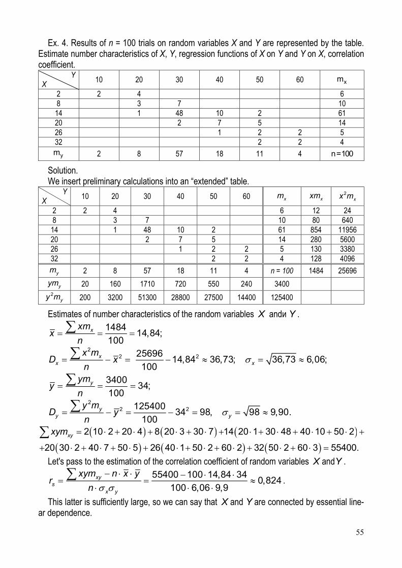
55

Ex. 4. Results of n = 100 trials on random variables X and Y are represented by the table. Estimate number characteristics of X, Y, regression functions of X on Y and Y on X, correlation coefficient.

Y X

10 20 30 40 50 60 xm

2 2 4 6 8 3 7 10 14 1 48 10 2 61 20 2 7 5 14 26 1 2 2 5 32 2 2 4

ym 2 8 57 18 11 4 n=100

Solution. We insert preliminary calculations into an “extended” table.

Y X

10 20 30 40 50 60 xm xxm 2xx m

2 2 4 6 12 24 8 3 7 10 80 640

14 1 48 10 2 61 854 11956 20 2 7 5 14 280 5600 26 1 2 2 5 130 3380 32 2 2 4 128 4096

ym 2 8 57 18 11 4 n = 100 1484 25696

yym 20 160 1710 720 550 240 3400 2

yy m 200 3200 51300 28800 27500 14400 125400

Estimates of number characteristics of the random variables X andи Y .

148414,84;

100xxm

xn

22 225696

14,84 36,73; 36,73 6,06;100

xx x

x mD x

n

340034;

100yym

yn

22 2125400

34 98, 98 9,90.100

yy y

y mD y

n

2 10 2 20 4 8 20 3 30 7 14 20 1 30 48 40 10 50 2

20 30 2 40 7 50 5 26 40 1 50 2 60 2 32 50 2 60 3 55400.

xyxym

Let's pass to the estimation of the correlation coefficient of random variables X andY . 55400 100 14,84 34

0,824100 6,06 9,9

xys

x y

xym n x yr

n

.

This latter is sufficiently large, so we can say that X and Y are connected by essential line-ar dependence.

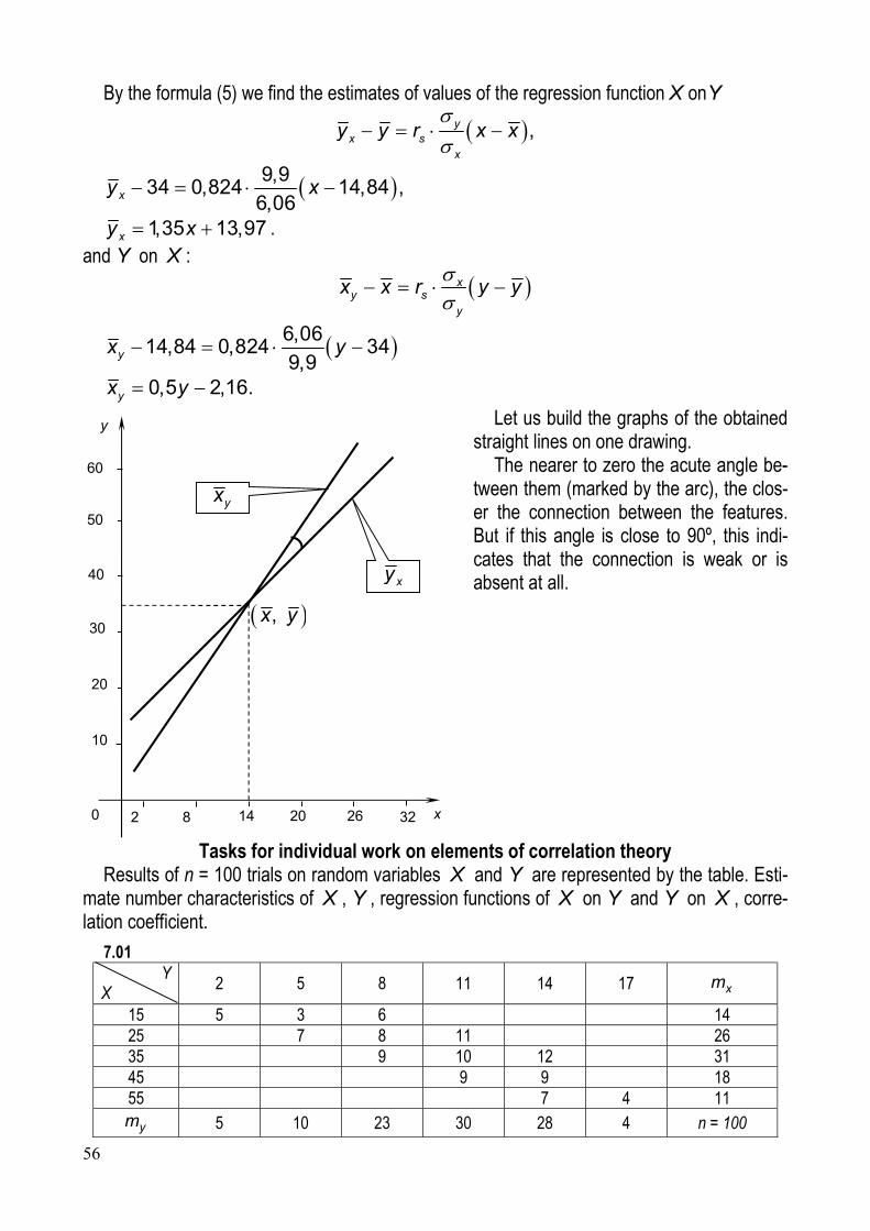
56

By the formula (5) we find the estimates of values of the regression function X onY

,yx s

x

y y r x x

9,9

34 0,824 14,84 ,6,06xy x

1,35 13,97xy x . and Y on X :

xy s

y

x x r y y

6,06

14,84 0,824 349,9yx y

0,5 2,16.yx y

Let us build the graphs of the obtained straight lines on one drawing.

The nearer to zero the acute angle be-tween them (marked by the arc), the clos-er the connection between the features. But if this angle is close to 90º, this indi-cates that the connection is weak or is absent at all.

Tasks for individual work on elements of correlation theory Results of n = 100 trials on random variables X and Y are represented by the table. Esti-

mate number characteristics of X , Y , regression functions of X on Y and Y on X , corre-lation coefficient.

7.01 Y

Х 2 5 8 11 14 17 xm

15 5 3 6 14 25 7 8 11 26 35 9 10 12 31 45 9 9 18 55 7 4 11

ym 5 10 23 30 28 4 n = 100

10

,x y

xy

yx

0

у

х

50

40

30

20

2 8 14 20 26

60

32

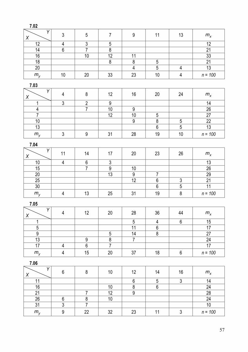
57

7.02 Y

Х 3 5 7 9 11 13 xm

12 4 3 5 12 14 6 7 8 21 16 10 12 11 33 18 8 8 5 21 20 4 5 4 13

ym 10 20 33 23 10 4 n = 100

7.03 Y

Х 4 8 12 16 20 24 xm

1 3 2 9 14 4 7 10 9 26 7 12 10 5 27

10 9 8 5 22 13 6 5 13

ym 3 9 31 28 19 10 n = 100

7.04 Y

Х 11 14 17 20 23 26 xm

10 4 6 3 13 15 7 9 10 26 20 13 9 7 29 25 12 6 3 21 30 6 5 11

ym 4 13 25 31 19 8 n = 100

7.05 Y

Х 4 12 20 28 36 44 xm

1 5 4 6 15 5 11 6 17 9 5 14 8 27

13 9 8 7 24 17 4 6 7 17

ym 4 15 20 37 18 6 n = 100

7.06 Y

Х 6 8 10 12 14 16 xm

11 6 5 3 14 16 10 8 6 24 21 7 12 9 28 26 6 8 10 24 31 3 7 10

ym 9 22 32 23 11 3 n = 100

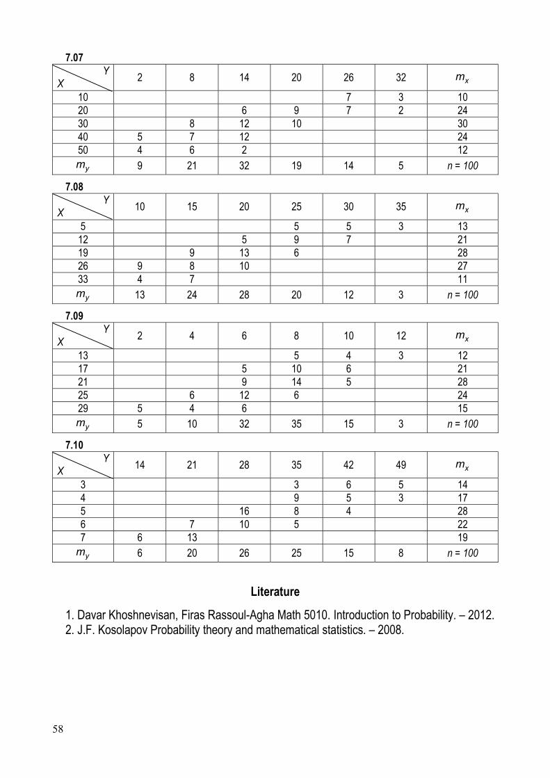
58

7.07 Y

Х 2 8 14 20 26 32 xm

10 7 3 10 20 6 9 7 2 24 30 8 12 10 30 40 5 7 12 24 50 4 6 2 12

ym 9 21 32 19 14 5 n = 100

7.08 Y

Х 10 15 20 25 30 35 xm

5 5 5 3 13 12 5 9 7 21 19 9 13 6 28 26 9 8 10 27 33 4 7 11

ym 13 24 28 20 12 3 n = 100

7.09 Y

Х 2 4 6 8 10 12 xm

13 5 4 3 12 17 5 10 6 21 21 9 14 5 28 25 6 12 6 24 29 5 4 6 15

ym 5 10 32 35 15 3 n = 100

7.10 Y

Х 14 21 28 35 42 49 xm

3 3 6 5 14 4 9 5 3 17 5 16 8 4 28 6 7 10 5 22 7 6 13 19

ym 6 20 26 25 15 8 n = 100

Literature

1. Davar Khoshnevisan, Firas Rassoul-Agha Math 5010. Introduction to Probability. – 2012. 2. J.F. Kosolapov Probability theory and mathematical statistics. – 2008.

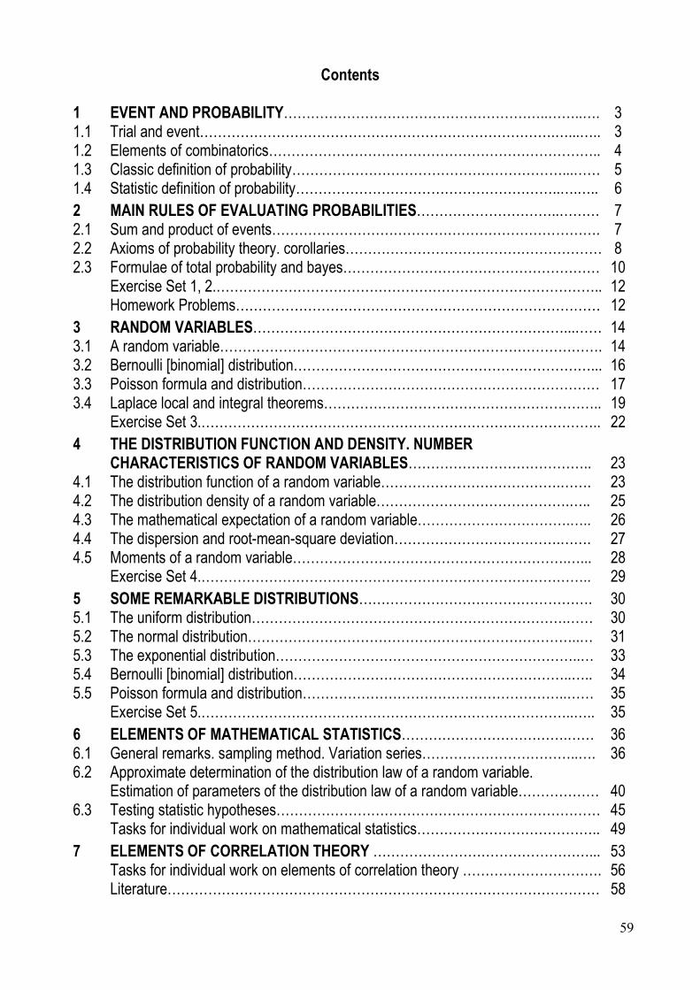
59

Contents

1 EVENT AND PROBABILITY…………………………………………………..……..…. 3 1.1 Trial and event…………………………………………………………………….…...….. 3 1.2 Elements of combinatorics……………………………………………………………….. 4 1.3 Classic definition of probability……………………………………………………...…… 5 1.4 Statistic definition of probability…………………………………………………..….….. 6 2 MAIN RULES OF EVALUATING PROBABILITIES…………………………..……… 7 2.1 Sum and product of events………………………………………………………………. 7 2.2 Axioms of probability theory. corollaries………………………………………………… 8 2.3 Formulae of total probability and bayes………………………………………………… 10 Exercise Set 1, 2.………………………………………………………………………….. 12 Homework Problems……………………………………………………………………… 12 3 RANDOM VARIABLES……………………………………………………………...…… 14 3.1 A random variable…………………………………………………………………………. 14 3.2 Bernoulli [binomial] distribution…………………………………………………………... 16 3.3 Poisson formula and distribution………………………………………………………… 17 3.4 Laplace local and integral theorems…………………………………………………….. 19 Exercise Set 3.…………………………………………………………………………….. 22 4 THE DISTRIBUTION FUNCTION AND DENSITY. NUMBER

CHARACTERISTICS OF RANDOM VARIABLES…………………………………..

23 4.1 The distribution function of a random variable………………………………….……. 23 4.2 The distribution density of a random variable…………………………………….….. 25 4.3 The mathematical expectation of a random variable…………………………….….. 26 4.4 The dispersion and root-mean-square deviation……………………………….……. 27 4.5 Moments of a random variable…………………………………………………….…... 28 Exercise Set 4.……………………………………………………………….………….. 29 5 SOME REMARKABLE DISTRIBUTIONS……………………………………………. 30 5.1 The uniform distribution…………………………………………………………….…… 30 5.2 The normal distribution………………………………………………………………..… 31 5.3 The exponential distribution…………………………………………………………..… 33 5.4 Bernoulli [binomial] distribution……………………………………………………..….. 34 5.5 Poisson formula and distribution…………………………………………………..…… 35 Exercise Set 5.………………………………………………………………………..….. 35 6 ELEMENTS OF MATHEMATICAL STATISTICS……………………………….…… 36 6.1 General remarks. sampling method. Variation series……………………………..…. 36 6.2 Approximate determination of the distribution law of a random variable.

Estimation of parameters of the distribution law of a random variable………………

40 6.3 Testing statistic hypotheses……………………………………………………………… 45 Tasks for individual work on mathematical statistics………………………………….. 49 7 ELEMENTS OF CORRELATION THEORY …………………………………………... 53 Tasks for individual work on elements of correlation theory …………………………. 56 Literature…………………………………………………………………………………… 58

УЧЕБНОЕ ИЗДАНИЕ

Составители: Гладкий Иван Иванович

Дворниченко Александр Валерьевич Каримова Татьяна Ивановна Лебедь Светлана Федоровна Шишко Татьяна Витальевна

PROBABILITY THEORY

ELEMENTS OF MATHEMATICAL STATISTICS

учебно-методическая разработка на английском языке

Ответственный за выпуск: Дворниченко А.В.

Редактор: Боровикова Е.А. Компьютерная верстка: Кармаш Е.Л.

Корректор: Шишко Т.В.

___________________________________________________________________________

Подписано к печати 24.09.2014 г. Формат 60х84 1/16. Бумага «Снегурочка». Усл. п. л. 3,49. Уч.-изд. л. 3,75. Заказ № 790. Тираж 40 экз.

Отпечатано на ризографе Учреждения образования «Брестский государственный технический университет».

224017, г. Брест, ул. Московская, 267.