Embed Size (px)
Citation preview
.
.
.
.
.
.
.
.
.
.
.
.
.
.
.
.
.
.
.
.
.
.
.
.
.
.
.
.
.
.
.
.
.
.
.
.
.
.
.
.
Write-optimization in external memory data structures
Leif Walsh
Tokutek, [email protected]
@leifwalsh
November 1, 2014
Leif Walsh (Tokutek) Fractal Trees November 1, 2014 1 / 31
.
.
.
.
.
.
.
.
.
.
.
.
.
.
.
.
.
.
.
.
.
.
.
.
.
.
.
.
.
.
.
.
.
.
.
.
.
.
.
.
Write-optimization in external memory data structures
Background
Leif Walsh (Tokutek) Fractal Trees November 1, 2014 2 / 31
.
.
.
.
.
.
.
.
.
.
.
.
.
.
.
.
.
.
.
.
.
.
.
.
.
.
.
.
.
.
.
.
.
.
.
.
.
.
.
.
Write-optimization in external memory data structures
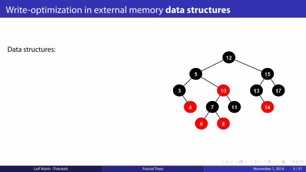
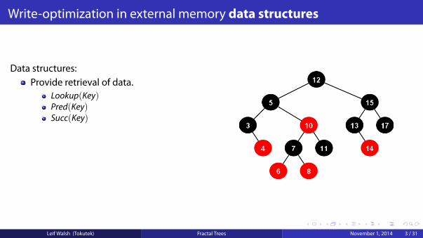
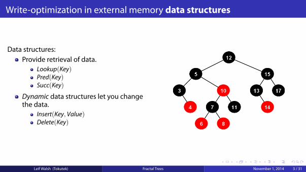
Data structures:
Provide retrieval of data.Lookup(Key)Pred(Key)Succ(Key)
Dynamic data structures let you changethe data.
Insert(Key, Value)Delete(Key)
Leif Walsh (Tokutek) Fractal Trees November 1, 2014 3 / 31
.
.
.
.
.
.
.
.
.
.
.
.
.
.
.
.
.
.
.
.
.
.
.
.
.
.
.
.
.
.
.
.
.
.
.
.
.
.
.
.
Write-optimization in external memory data structures
Data structures:Provide retrieval of data.
Lookup(Key)Pred(Key)Succ(Key)
Dynamic data structures let you changethe data.
Insert(Key, Value)Delete(Key)
Leif Walsh (Tokutek) Fractal Trees November 1, 2014 3 / 31
.
.
.
.
.
.
.
.
.
.
.
.
.
.
.
.
.
.
.
.
.
.
.
.
.
.
.
.
.
.
.
.
.
.
.
.
.
.
.
.
Write-optimization in external memory data structures
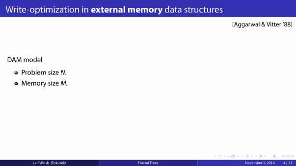
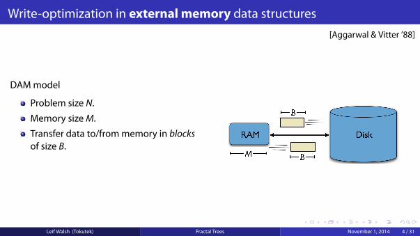
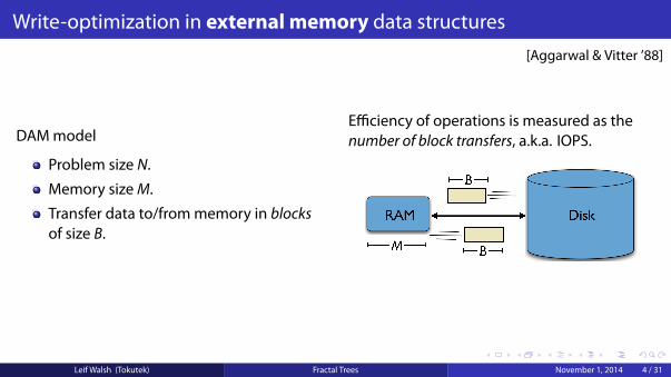
DAM model
Problem size N.
Memory sizeM.
Transfer data to/from memory in blocksof size B.
Efficiency of operations is measured as thenumber of block transfers, a.k.a. IOPS.
Leif Walsh (Tokutek) Fractal Trees November 1, 2014 4 / 31
[Aggarwal & Vitter ’88]
.
.
.
.
.
.
.
.
.
.
.
.
.
.
.
.
.
.
.
.
.
.
.
.
.
.
.
.
.
.
.
.
.
.
.
.
.
.
.
.
Write-optimization in external memory data structures
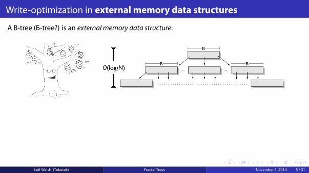
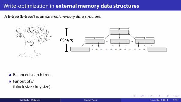
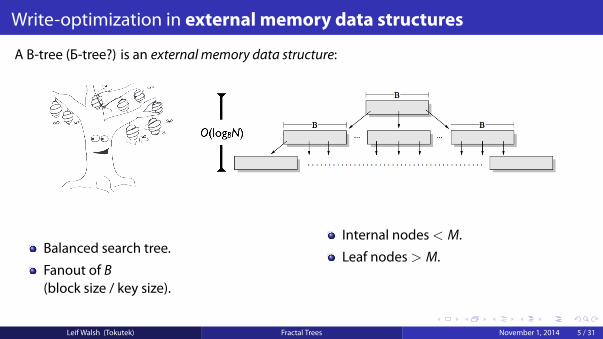
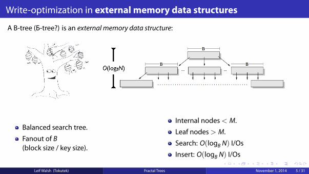
A B-tree (Б-tree?) is an external memory data structure:
Balanced search tree.
Fanout of B(block size / key size).
Internal nodes< M.
Leaf nodes> M.
Search: O(logB N) I/Os
Insert: O(logB N) I/Os
Leif Walsh (Tokutek) Fractal Trees November 1, 2014 5 / 31
.
.
.
.
.
.
.
.
.
.
.
.
.
.
.
.
.
.
.
.
.
.
.
.
.
.
.
.
.
.
.
.
.
.
.
.
.
.
.
.
Write-optimization in external memory data structures
Leif Walsh (Tokutek) Fractal Trees November 1, 2014 6 / 31
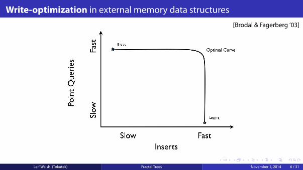
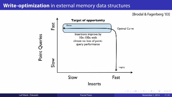
[Brodal & Fagerberg ’03]
.
.
.
.
.
.
.
.
.
.
.
.
.
.
.
.
.
.
.
.
.
.
.
.
.
.
.
.
.
.
.
.
.
.
.
.
.
.
.
.
Write-optimization in external memory data structures
Leif Walsh (Tokutek) Fractal Trees November 1, 2014 7 / 31
[Brodal & Fagerberg ’03]
.
.
.
.
.
.
.
.
.
.
.
.
.
.
.
.
.
.
.
.
.
.
.
.
.
.
.
.
.
.
.
.
.
.
.
.
.
.
.
.
Write-optimization in external memory data structures
OLAP
Leif Walsh (Tokutek) Fractal Trees November 1, 2014 8 / 31

.
.
.
.
.
.
.
.
.
.
.
.
.
.
.
.
.
.
.
.
.
.
.
.
.
.
.
.
.
.
.
.
.
.
.
.
.
.
.
.
Write-optimization technique #1: OLAP
OLAP: Online Analytical Processing
Key idea: Analyze data collected in the past.B-tree inserts are slow, but…logging and sorting are fast.
Leif Walsh (Tokutek) Fractal Trees November 1, 2014 9 / 31

.
.
.
.
.
.
.
.
.
.
.
.
.
.
.
.
.
.
.
.
.
.
.
.
.
.
.
.
.
.
.
.
.
.
.
.
.
.
.
.
Write-optimization technique #1: OLAP
OLAP: Online Analytical ProcessingKey idea: Analyze data collected in the past.
B-tree inserts are slow, but…logging and sorting are fast.
Leif Walsh (Tokutek) Fractal Trees November 1, 2014 9 / 31
.
.
.
.
.
.
.
.
.
.
.
.
.
.
.
.
.
.
.
.
.
.
.
.
.
.
.
.
.
.
.
.
.
.
.
.
.
.
.
.
Write-optimization technique #1: OLAP
OLAP: Online Analytical ProcessingKey idea: Analyze data collected in the past.B-tree inserts are slow, but…logging and sorting are fast.
Leif Walsh (Tokutek) Fractal Trees November 1, 2014 9 / 31
.
.
.
.
.
.
.
.
.
.
.
.
.
.
.
.
.
.
.
.
.
.
.
.
.
.
.
.
.
.
.
.
.
.
.
.
.
.
.
.
Write-optimization technique #1: OLAP
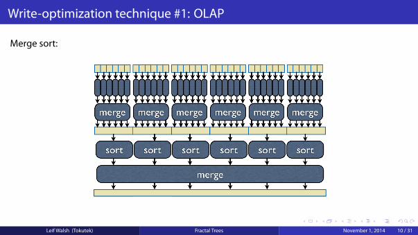
Merge sort:
Leif Walsh (Tokutek) Fractal Trees November 1, 2014 10 / 31
.
.
.
.
.
.
.
.
.
.
.
.
.
.
.
.
.
.
.
.
.
.
.
.
.
.
.
.
.
.
.
.
.
.
.
.
.
.
.
.
Write-optimization technique #1: OLAP
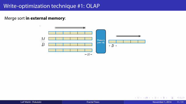
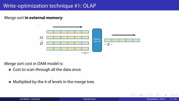
Merge sort in external memory:
Merge sort cost in DAM model is:Cost to scan through all the data once.
N/B
Multiplied by the # of levels in the merge tree.
logM/B N/B
O(NBlogM/B
NB
)
Leif Walsh (Tokutek) Fractal Trees November 1, 2014 11 / 31
.
.
.
.
.
.
.
.
.
.
.
.
.
.
.
.
.
.
.
.
.
.
.
.
.
.
.
.
.
.
.
.
.
.
.
.
.
.
.
.
Write-optimization technique #1: OLAP
Merge sort in external memory:
Merge sort cost in DAM model is:Cost to scan through all the data once.
N/B
Multiplied by the # of levels in the merge tree.
logM/B N/B
O(NBlogM/B
NB
)
Leif Walsh (Tokutek) Fractal Trees November 1, 2014 11 / 31

.
.
.
.
.
.
.
.
.
.
.
.
.
.
.
.
.
.
.
.
.
.
.
.
.
.
.
.
.
.
.
.
.
.
.
.
.
.
.
.
Write-optimization technique #1: OLAP
Merge sort in external memory:
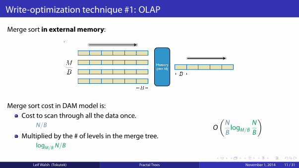
Merge sort cost in DAM model is:Cost to scan through all the data once.
N/B
Multiplied by the # of levels in the merge tree.logM/B N/B
O(NBlogM/B
NB
)
Leif Walsh (Tokutek) Fractal Trees November 1, 2014 11 / 31
.
.
.
.
.
.
.
.
.
.
.
.
.
.
.
.
.
.
.
.
.
.
.
.
.
.
.
.
.
.
.
.
.
.
.
.
.
.
.
.
Write-optimization technique #1: OLAP
Merge sort in external memory:
Merge sort cost in DAM model is:Cost to scan through all the data once.
N/B
Multiplied by the # of levels in the merge tree.logM/B N/B
O(NBlogM/B
NB
)
Leif Walsh (Tokutek) Fractal Trees November 1, 2014 11 / 31

.
.
.
.
.
.
.
.
.
.
.
.
.
.
.
.
.
.
.
.
.
.
.
.
.
.
.
.
.
.
.
.
.
.
.
.
.
.
.
.
Write-optimization technique #1: OLAP
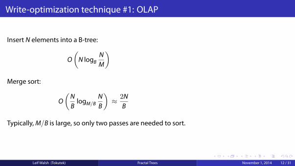
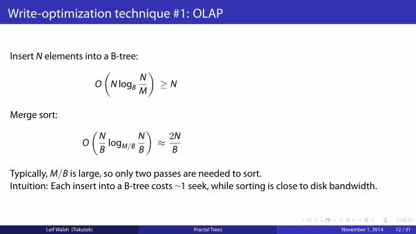
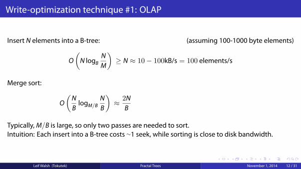
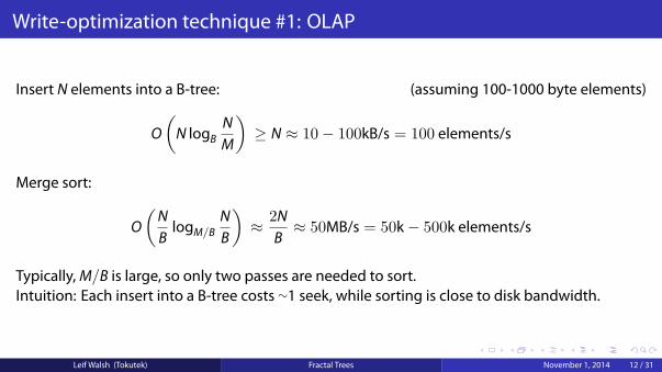
Insert N elements into a B-tree:
(assuming 100-1000 byte elements)
O(N logB
NM
)
≥ N ≈ 10− 100kB/s = 100 elements/s
Merge sort:
O(NB
logM/BNB
)
≈ 2NB
≈ 50MB/s = 50k− 500k elements/s
Typically,M/B is large, so only two passes are needed to sort.Intuition: Each insert into a B-tree costs ∼1 seek, while sorting is close to disk bandwidth.
Leif Walsh (Tokutek) Fractal Trees November 1, 2014 12 / 31
.
.
.
.
.
.
.
.
.
.
.
.
.
.
.
.
.
.
.
.
.
.
.
.
.
.
.
.
.
.
.
.
.
.
.
.
.
.
.
.
Write-optimization technique #1: OLAP
Insert N elements into a B-tree:
(assuming 100-1000 byte elements)
O(N logB
NM
)
≥ N ≈ 10− 100kB/s = 100 elements/s
Merge sort:
O(NB
logM/BNB
)≈ 2N
B
≈ 50MB/s = 50k− 500k elements/s
Typically,M/B is large, so only two passes are needed to sort.
Intuition: Each insert into a B-tree costs ∼1 seek, while sorting is close to disk bandwidth.
Leif Walsh (Tokutek) Fractal Trees November 1, 2014 12 / 31
.
.
.
.
.
.
.
.
.
.
.
.
.
.
.
.
.
.
.
.
.
.
.
.
.
.
.
.
.
.
.
.
.
.
.
.
.
.
.
.
Write-optimization technique #1: OLAP
Insert N elements into a B-tree:
(assuming 100-1000 byte elements)
O(N logB
NM
)≥ N
≈ 10− 100kB/s = 100 elements/s
Merge sort:
O(NB
logM/BNB
)≈ 2N
B
≈ 50MB/s = 50k− 500k elements/s
Typically,M/B is large, so only two passes are needed to sort.Intuition: Each insert into a B-tree costs ∼1 seek, while sorting is close to disk bandwidth.
Leif Walsh (Tokutek) Fractal Trees November 1, 2014 12 / 31
.
.
.
.
.
.
.
.
.
.
.
.
.
.
.
.
.
.
.
.
.
.
.
.
.
.
.
.
.
.
.
.
.
.
.
.
.
.
.
.
Write-optimization technique #1: OLAP
Insert N elements into a B-tree: (assuming 100-1000 byte elements)
O(N logB
NM
)≥ N ≈ 10− 100kB/s = 100 elements/s
Merge sort:
O(NB
logM/BNB
)≈ 2N
B≈ 50MB/s = 50k− 500k elements/s
Typically,M/B is large, so only two passes are needed to sort.Intuition: Each insert into a B-tree costs ∼1 seek, while sorting is close to disk bandwidth.
Leif Walsh (Tokutek) Fractal Trees November 1, 2014 12 / 31

.
.
.
.
.
.
.
.
.
.
.
.
.
.
.
.
.
.
.
.
.
.
.
.
.
.
.
.
.
.
.
.
.
.
.
.
.
.
.
.
Write-optimization technique #1: OLAP
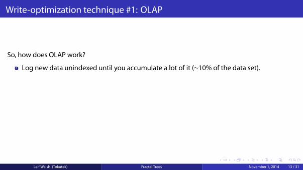
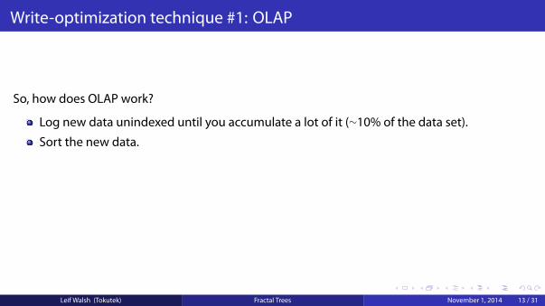
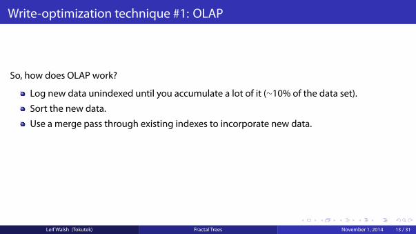
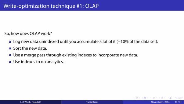
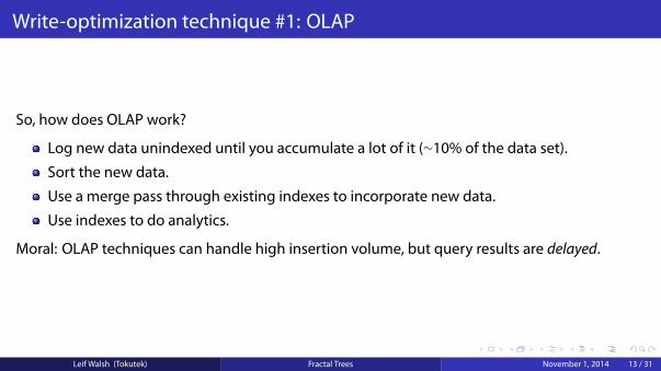
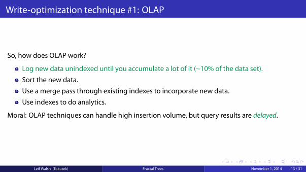
So, how does OLAP work?
Log new data unindexed until you accumulate a lot of it (∼10% of the data set).
Sort the new data.
Use a merge pass through existing indexes to incorporate new data.
Use indexes to do analytics.
Moral: OLAP techniques can handle high insertion volume, but query results are delayed.
Leif Walsh (Tokutek) Fractal Trees November 1, 2014 13 / 31
.
.
.
.
.
.
.
.
.
.
.
.
.
.
.
.
.
.
.
.
.
.
.
.
.
.
.
.
.
.
.
.
.
.
.
.
.
.
.
.
Write-optimization technique #1: OLAP
So, how does OLAP work?
Log new data unindexed until you accumulate a lot of it (∼10% of the data set).
Sort the new data.
Use a merge pass through existing indexes to incorporate new data.
Use indexes to do analytics.
Moral: OLAP techniques can handle high insertion volume, but query results are delayed.
Leif Walsh (Tokutek) Fractal Trees November 1, 2014 13 / 31
.
.
.
.
.
.
.
.
.
.
.
.
.
.
.
.
.
.
.
.
.
.
.
.
.
.
.
.
.
.
.
.
.
.
.
.
.
.
.
.
Write-optimization in external memory data structures
LSM-trees
Leif Walsh (Tokutek) Fractal Trees November 1, 2014 14 / 31
.
.
.
.
.
.
.
.
.
.
.
.
.
.
.
.
.
.
.
.
.
.
.
.
.
.
.
.
.
.
.
.
.
.
.
.
.
.
.
.
Write-optimization technique #2: LSM-trees
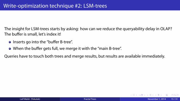
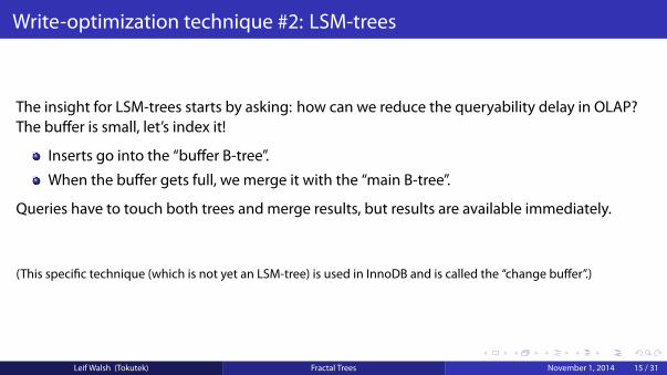
The insight for LSM-trees starts by asking: how can we reduce the queryability delay in OLAP?
The buffer is small, let’s index it!
Inserts go into the “buffer B-tree”.
When the buffer gets full, we merge it with the “main B-tree”.
Queries have to touch both trees and merge results, but results are available immediately.
(This specific technique (which is not yet an LSM-tree) is used in InnoDB and is called the “change buffer”.)
Leif Walsh (Tokutek) Fractal Trees November 1, 2014 15 / 31
.
.
.
.
.
.
.
.
.
.
.
.
.
.
.
.
.
.
.
.
.
.
.
.
.
.
.
.
.
.
.
.
.
.
.
.
.
.
.
.
Write-optimization technique #2: LSM-trees
The insight for LSM-trees starts by asking: how can we reduce the queryability delay in OLAP?The buffer is small, let’s index it!
Inserts go into the “buffer B-tree”.
When the buffer gets full, we merge it with the “main B-tree”.
Queries have to touch both trees and merge results, but results are available immediately.
(This specific technique (which is not yet an LSM-tree) is used in InnoDB and is called the “change buffer”.)
Leif Walsh (Tokutek) Fractal Trees November 1, 2014 15 / 31
.
.
.
.
.
.
.
.
.
.
.
.
.
.
.
.
.
.
.
.
.
.
.
.
.
.
.
.
.
.
.
.
.
.
.
.
.
.
.
.
Write-optimization technique #2: LSM-trees
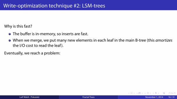
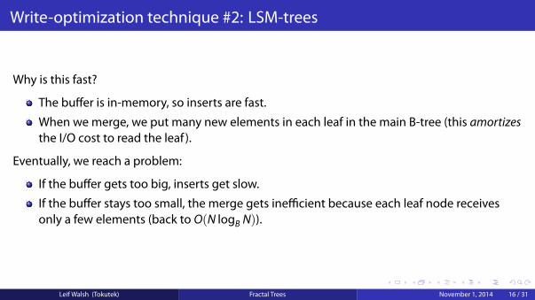
Why is this fast?
The buffer is in-memory, so inserts are fast.
When we merge, we put many new elements in each leaf in the main B-tree (this amortizesthe I/O cost to read the leaf ).
Eventually, we reach a problem:
If the buffer gets too big, inserts get slow.
If the buffer stays too small, the merge gets inefficient because each leaf node receivesonly a few elements (back to O(N logB N)).
Leif Walsh (Tokutek) Fractal Trees November 1, 2014 16 / 31
.
.
.
.
.
.
.
.
.
.
.
.
.
.
.
.
.
.
.
.
.
.
.
.
.
.
.
.
.
.
.
.
.
.
.
.
.
.
.
.
Write-optimization technique #2: LSM-trees
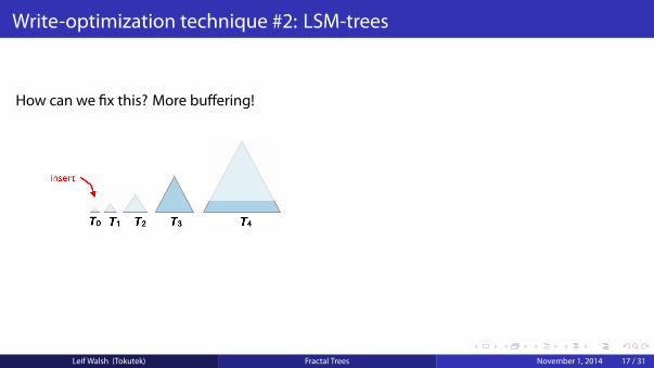
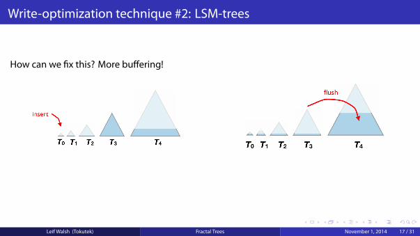
How can we fix this?
More buffering!
Each level is twice as large as the previous level, for some value of 2 (usually 10). We’ll use 2.
Leif Walsh (Tokutek) Fractal Trees November 1, 2014 17 / 31
.
.
.
.
.
.
.
.
.
.
.
.
.
.
.
.
.
.
.
.
.
.
.
.
.
.
.
.
.
.
.
.
.
.
.
.
.
.
.
.
Write-optimization technique #2: LSM-trees
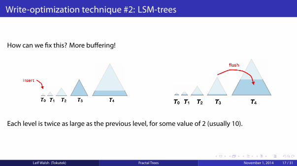
How can we fix this? More buffering!
Each level is twice as large as the previous level, for some value of 2 (usually 10). We’ll use 2.
Leif Walsh (Tokutek) Fractal Trees November 1, 2014 17 / 31
.
.
.
.
.
.
.
.
.
.
.
.
.
.
.
.
.
.
.
.
.
.
.
.
.
.
.
.
.
.
.
.
.
.
.
.
.
.
.
.
Write-optimization technique #2: LSM-trees
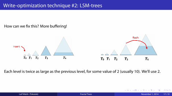
How can we fix this? More buffering!
Each level is twice as large as the previous level, for some value of 2 (usually 10).
We’ll use 2.
Leif Walsh (Tokutek) Fractal Trees November 1, 2014 17 / 31
.
.
.
.
.
.
.
.
.
.
.
.
.
.
.
.
.
.
.
.
.
.
.
.
.
.
.
.
.
.
.
.
.
.
.
.
.
.
.
.
Write-optimization technique #2: LSM-trees
How can we fix this? More buffering!
Each level is twice as large as the previous level, for some value of 2 (usually 10). We’ll use 2.
Leif Walsh (Tokutek) Fractal Trees November 1, 2014 17 / 31
.
.
.
.
.
.
.
.
.
.
.
.
.
.
.
.
.
.
.
.
.
.
.
.
.
.
.
.
.
.
.
.
.
.
.
.
.
.
.
.
Write-optimization technique #2: LSM-trees
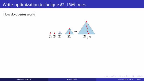
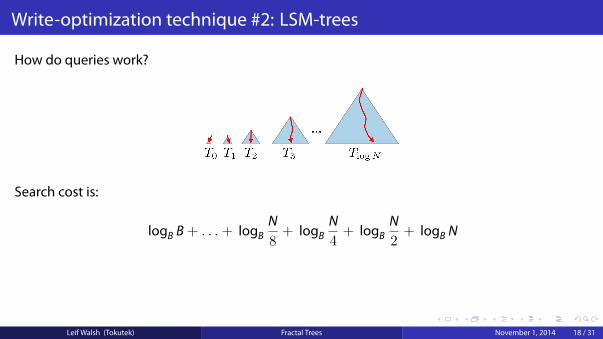
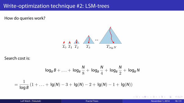
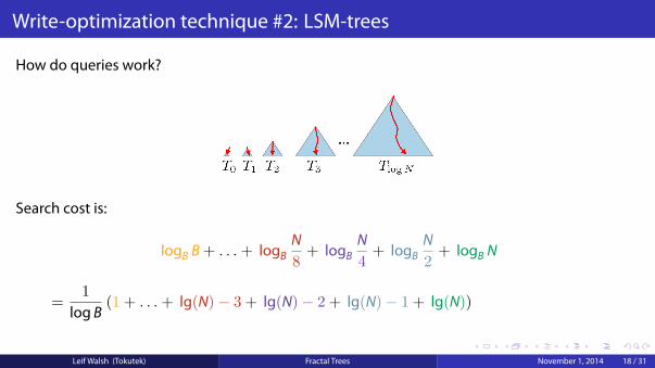
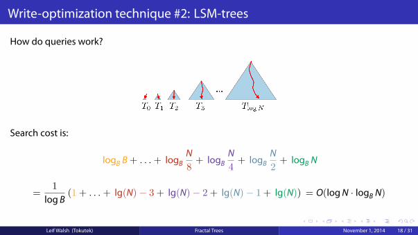
How do queries work?
Search cost is:
logB B+ . . .+ logBN8+ logB
N4+ logB
N2+ logB N
=1
log B(1 + . . .+ lg(N)− 3 + lg(N)− 2 + lg(N)− 1 + lg(N))
= O(logN · logB N)
Leif Walsh (Tokutek) Fractal Trees November 1, 2014 18 / 31
.
.
.
.
.
.
.
.
.
.
.
.
.
.
.
.
.
.
.
.
.
.
.
.
.
.
.
.
.
.
.
.
.
.
.
.
.
.
.
.
Write-optimization technique #2: LSM-trees
How do queries work?
Search cost is:
logB B+ . . .+ logBN8+ logB
N4+ logB
N2+ logB N
=1
log B(1 + . . .+ lg(N)− 3 + lg(N)− 2 + lg(N)− 1 + lg(N)) = O(logN · logB N)
Leif Walsh (Tokutek) Fractal Trees November 1, 2014 18 / 31
.
.
.
.
.
.
.
.
.
.
.
.
.
.
.
.
.
.
.
.
.
.
.
.
.
.
.
.
.
.
.
.
.
.
.
.
.
.
.
.
Write-optimization technique #2: LSM-trees
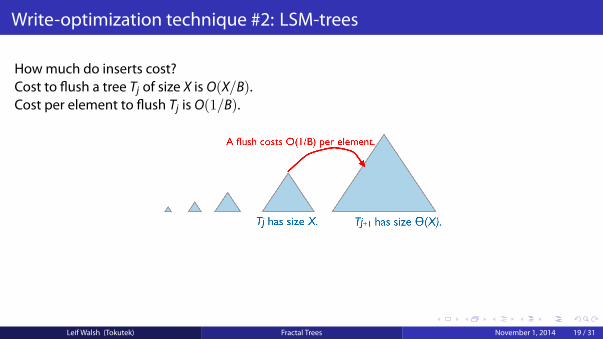
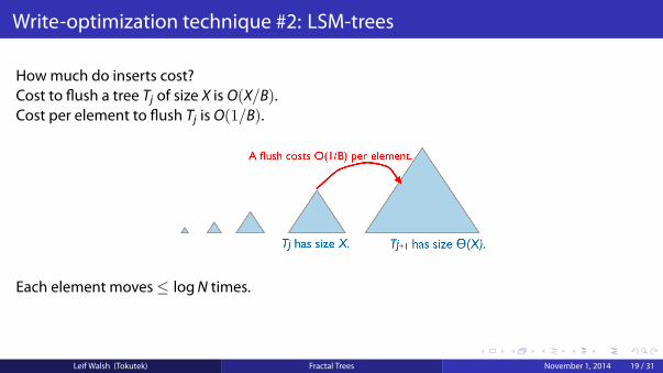
How much do inserts cost?
Cost to flush a tree Tj of size X is O(X/B).Cost per element to flush Tj is O(1/B).
Each element moves≤ logN times.Total amortized insert cost per element is O
(logNB
).
Leif Walsh (Tokutek) Fractal Trees November 1, 2014 19 / 31
.
.
.
.
.
.
.
.
.
.
.
.
.
.
.
.
.
.
.
.
.
.
.
.
.
.
.
.
.
.
.
.
.
.
.
.
.
.
.
.
Write-optimization technique #2: LSM-trees
How much do inserts cost?Cost to flush a tree Tj of size X is O(X/B).
Cost per element to flush Tj is O(1/B).
Each element moves≤ logN times.Total amortized insert cost per element is O
(logNB
).
Leif Walsh (Tokutek) Fractal Trees November 1, 2014 19 / 31
.
.
.
.
.
.
.
.
.
.
.
.
.
.
.
.
.
.
.
.
.
.
.
.
.
.
.
.
.
.
.
.
.
.
.
.
.
.
.
.
Write-optimization technique #2: LSM-trees
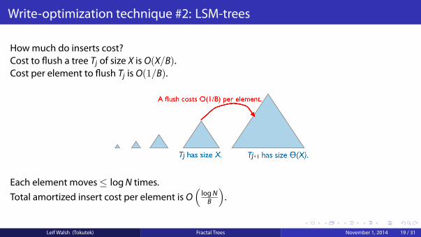
How much do inserts cost?Cost to flush a tree Tj of size X is O(X/B).Cost per element to flush Tj is O(1/B).
Each element moves≤ logN times.Total amortized insert cost per element is O
(logNB
).
Leif Walsh (Tokutek) Fractal Trees November 1, 2014 19 / 31
.
.
.
.
.
.
.
.
.
.
.
.
.
.
.
.
.
.
.
.
.
.
.
.
.
.
.
.
.
.
.
.
.
.
.
.
.
.
.
.
Write-optimization technique #2: LSM-trees
How much do inserts cost?Cost to flush a tree Tj of size X is O(X/B).Cost per element to flush Tj is O(1/B).
Each element moves≤ logN times.
Total amortized insert cost per element is O(
logNB
).
Leif Walsh (Tokutek) Fractal Trees November 1, 2014 19 / 31
.
.
.
.
.
.
.
.
.
.
.
.
.
.
.
.
.
.
.
.
.
.
.
.
.
.
.
.
.
.
.
.
.
.
.
.
.
.
.
.
Write-optimization technique #2: LSM-trees
How much do inserts cost?Cost to flush a tree Tj of size X is O(X/B).Cost per element to flush Tj is O(1/B).
Each element moves≤ logN times.Total amortized insert cost per element is O
(logNB
).
Leif Walsh (Tokutek) Fractal Trees November 1, 2014 19 / 31
.
.
.
.
.
.
.
.
.
.
.
.
.
.
.
.
.
.
.
.
.
.
.
.
.
.
.
.
.
.
.
.
.
.
.
.
.
.
.
.
Write-optimization in external memory data structures
Fractal Trees
Leif Walsh (Tokutek) Fractal Trees November 1, 2014 20 / 31
.
.
.
.
.
.
.
.
.
.
.
.
.
.
.
.
.
.
.
.
.
.
.
.
.
.
.
.
.
.
.
.
.
.
.
.
.
.
.
.
Write-optimization technique #3: Fractal Trees
The pain in LSM-trees is doing a full O(logB N) search in each level.
We use fractional cascading to reduce the search per level to O(1).
The idea is that once we’ve searched Ti, we know where the key would be in Ti, and we can usethat information to guide our search of Ti+1.
Leif Walsh (Tokutek) Fractal Trees November 1, 2014 21 / 31
.
.
.
.
.
.
.
.
.
.
.
.
.
.
.
.
.
.
.
.
.
.
.
.
.
.
.
.
.
.
.
.
.
.
.
.
.
.
.
.
Write-optimization technique #3: Fractal Trees
The pain in LSM-trees is doing a full O(logB N) search in each level.We use fractional cascading to reduce the search per level to O(1).
The idea is that once we’ve searched Ti, we know where the key would be in Ti, and we can usethat information to guide our search of Ti+1.
Leif Walsh (Tokutek) Fractal Trees November 1, 2014 21 / 31
.
.
.
.
.
.
.
.
.
.
.
.
.
.
.
.
.
.
.
.
.
.
.
.
.
.
.
.
.
.
.
.
.
.
.
.
.
.
.
.
Write-optimization technique #3: Fractal Trees
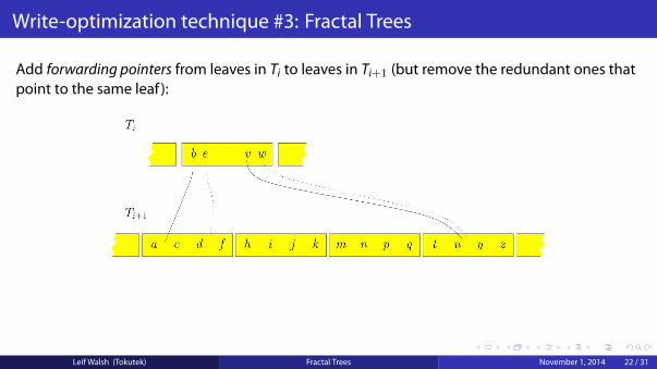
Add forwarding pointers from leaves in Ti to leaves in Ti+1 (but remove the redundant ones thatpoint to the same leaf ):
Leif Walsh (Tokutek) Fractal Trees November 1, 2014 22 / 31
.
.
.
.
.
.
.
.
.
.
.
.
.
.
.
.
.
.
.
.
.
.
.
.
.
.
.
.
.
.
.
.
.
.
.
.
.
.
.
.
Write-optimization technique #3: Fractal Trees
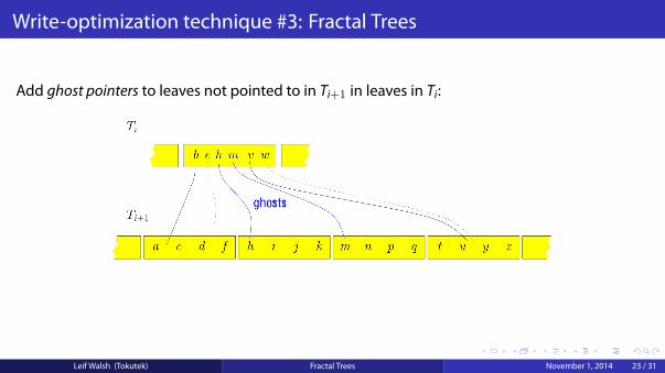
Add ghost pointers to leaves not pointed to in Ti+1 in leaves in Ti:
Leif Walsh (Tokutek) Fractal Trees November 1, 2014 23 / 31
.
.
.
.
.
.
.
.
.
.
.
.
.
.
.
.
.
.
.
.
.
.
.
.
.
.
.
.
.
.
.
.
.
.
.
.
.
.
.
.
Write-optimization technique #3: Fractal Trees
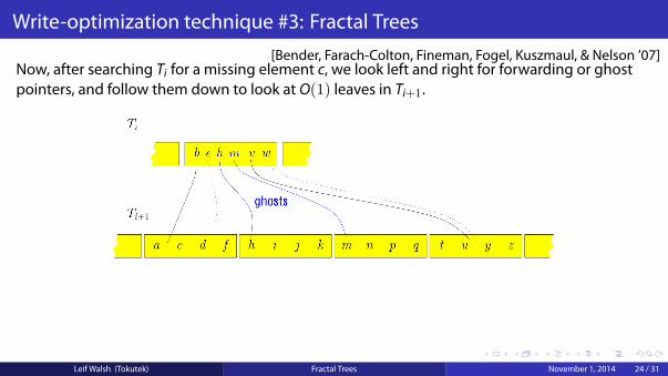
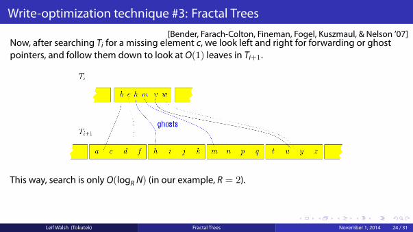
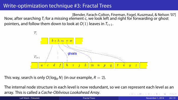
Now, after searching Ti for a missing element c, we look left and right for forwarding or ghostpointers, and follow them down to look at O(1) leaves in Ti+1.
This way, search is only O(logR N) (in our example, R = 2).
The internal node structure in each level is now redundant, so we can represent each level as anarray. This is called a Cache-Oblivious Lookahead Array.
Leif Walsh (Tokutek) Fractal Trees November 1, 2014 24 / 31
[Bender, Farach-Colton, Fineman, Fogel, Kuszmaul, & Nelson ’07]
.
.
.
.
.
.
.
.
.
.
.
.
.
.
.
.
.
.
.
.
.
.
.
.
.
.
.
.
.
.
.
.
.
.
.
.
.
.
.
.
Write-optimization technique #3: Fractal Trees
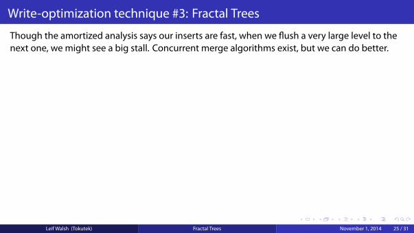
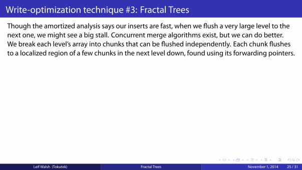
Though the amortized analysis says our inserts are fast, when we flush a very large level to thenext one, we might see a big stall. Concurrent merge algorithms exist, but we can do better.
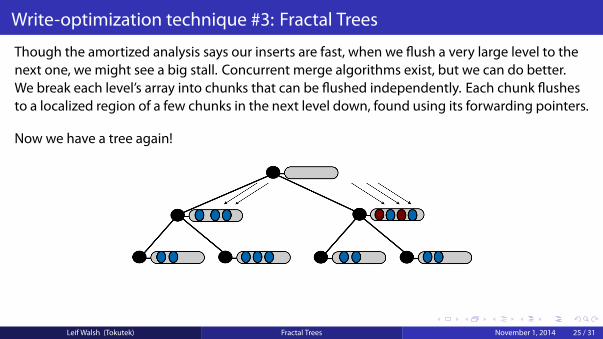
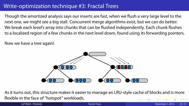
We break each level’s array into chunks that can be flushed independently. Each chunk flushesto a localized region of a few chunks in the next level down, found using its forwarding pointers.
Now we have a tree again!
As it turns out, this structure makes it easier to manage an LRU-style cache of blocks and is moreflexible in the face of “hotspot” workloads.
Leif Walsh (Tokutek) Fractal Trees November 1, 2014 25 / 31
.
.
.
.
.
.
.
.
.
.
.
.
.
.
.
.
.
.
.
.
.
.
.
.
.
.
.
.
.
.
.
.
.
.
.
.
.
.
.
.
Write-optimization technique #3: Fractal Trees
Though the amortized analysis says our inserts are fast, when we flush a very large level to thenext one, we might see a big stall. Concurrent merge algorithms exist, but we can do better.We break each level’s array into chunks that can be flushed independently. Each chunk flushesto a localized region of a few chunks in the next level down, found using its forwarding pointers.
Now we have a tree again!
As it turns out, this structure makes it easier to manage an LRU-style cache of blocks and is moreflexible in the face of “hotspot” workloads.
Leif Walsh (Tokutek) Fractal Trees November 1, 2014 25 / 31
.
.
.
.
.
.
.
.
.
.
.
.
.
.
.
.
.
.
.
.
.
.
.
.
.
.
.
.
.
.
.
.
.
.
.
.
.
.
.
.
Results
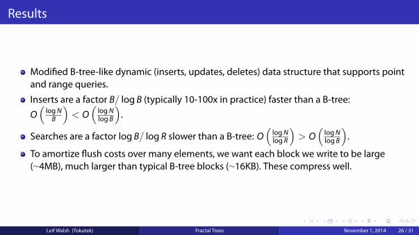
Modified B-tree-like dynamic (inserts, updates, deletes) data structure that supports pointand range queries.
Inserts are a factor B/ log B (typically 10-100x in practice) faster than a B-tree:O(
logNB
)< O
(logNlog B
).
Searches are a factor log B/ log R slower than a B-tree: O(
logNlog R
)> O
(logNlog B
).
To amortize flush costs over many elements, we want each block we write to be large(∼4MB), much larger than typical B-tree blocks (∼16KB). These compress well.
Leif Walsh (Tokutek) Fractal Trees November 1, 2014 26 / 31
.
.
.
.
.
.
.
.
.
.
.
.
.
.
.
.
.
.
.
.
.
.
.
.
.
.
.
.
.
.
.
.
.
.
.
.
.
.
.
.
Applications
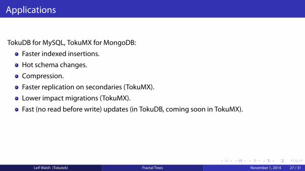
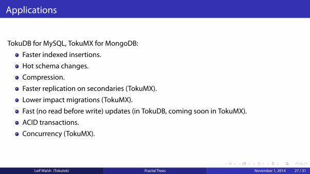
TokuDB for MySQL, TokuMX for MongoDB:
Faster indexed insertions.
Hot schema changes.
Compression.
Faster replication on secondaries (TokuMX).
Lower impact migrations (TokuMX).
Fast (no read before write) updates (in TokuDB, coming soon in TokuMX).
ACID transactions.
Concurrency (TokuMX).
Leif Walsh (Tokutek) Fractal Trees November 1, 2014 27 / 31
.
.
.
.
.
.
.
.
.
.
.
.
.
.
.
.
.
.
.
.
.
.
.
.
.
.
.
.
.
.
.
.
.
.
.
.
.
.
.
.
Applications
TokuDB for MySQL, TokuMX for MongoDB:
Faster indexed insertions.
Hot schema changes.
Compression.
Faster replication on secondaries (TokuMX).
Lower impact migrations (TokuMX).
Fast (no read before write) updates (in TokuDB, coming soon in TokuMX).
ACID transactions.
Concurrency (TokuMX).
Leif Walsh (Tokutek) Fractal Trees November 1, 2014 27 / 31
.
.
.
.
.
.
.
.
.
.
.
.
.
.
.
.
.
.
.
.
.
.
.
.
.
.
.
.
.
.
.
.
.
.
.
.
.
.
.
.
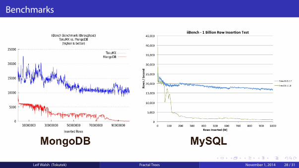
Benchmarks
Leif Walsh (Tokutek) Fractal Trees November 1, 2014 28 / 31
.
.
.
.
.
.
.
.
.
.
.
.
.
.
.
.
.
.
.
.
.
.
.
.
.
.
.
.
.
.
.
.
.
.
.
.
.
.
.
.
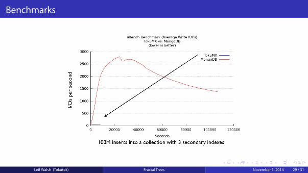
Benchmarks
Leif Walsh (Tokutek) Fractal Trees November 1, 2014 29 / 31
.
.
.
.
.
.
.
.
.
.
.
.
.
.
.
.
.
.
.
.
.
.
.
.
.
.
.
.
.
.
.
.
.
.
.
.
.
.
.
.
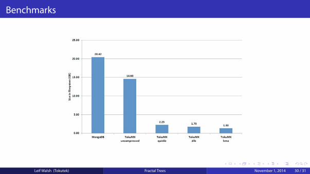
Benchmarks
Leif Walsh (Tokutek) Fractal Trees November 1, 2014 30 / 31
.
.
.
.
.
.
.
.
.
.
.
.
.
.
.
.
.
.
.
.
.
.
.
.
.
.
.
.
.
.
.
.
.
.
.
.
.
.
.
.
Questions?
Leif [email protected]
@leifwalshDownloads: www.tokutek.com/downloads
Docs: docs.tokutek.comSlides: slidesha.re/1tqwORg
Leif Walsh (Tokutek) Fractal Trees November 1, 2014 31 / 31