Embed Size (px)
Citation preview
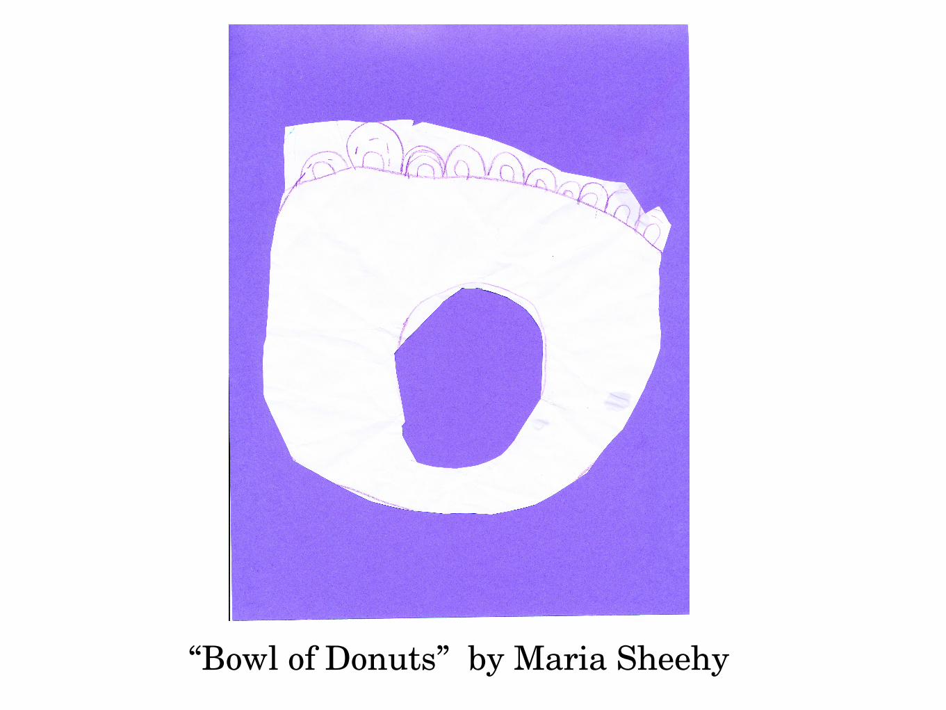
“Bowl of Donuts” by Maria Sheehy

Sensors and Samples: A Homological Approach
Nick Cavanna, Kirk Gardner, and Don Sheehy UConn

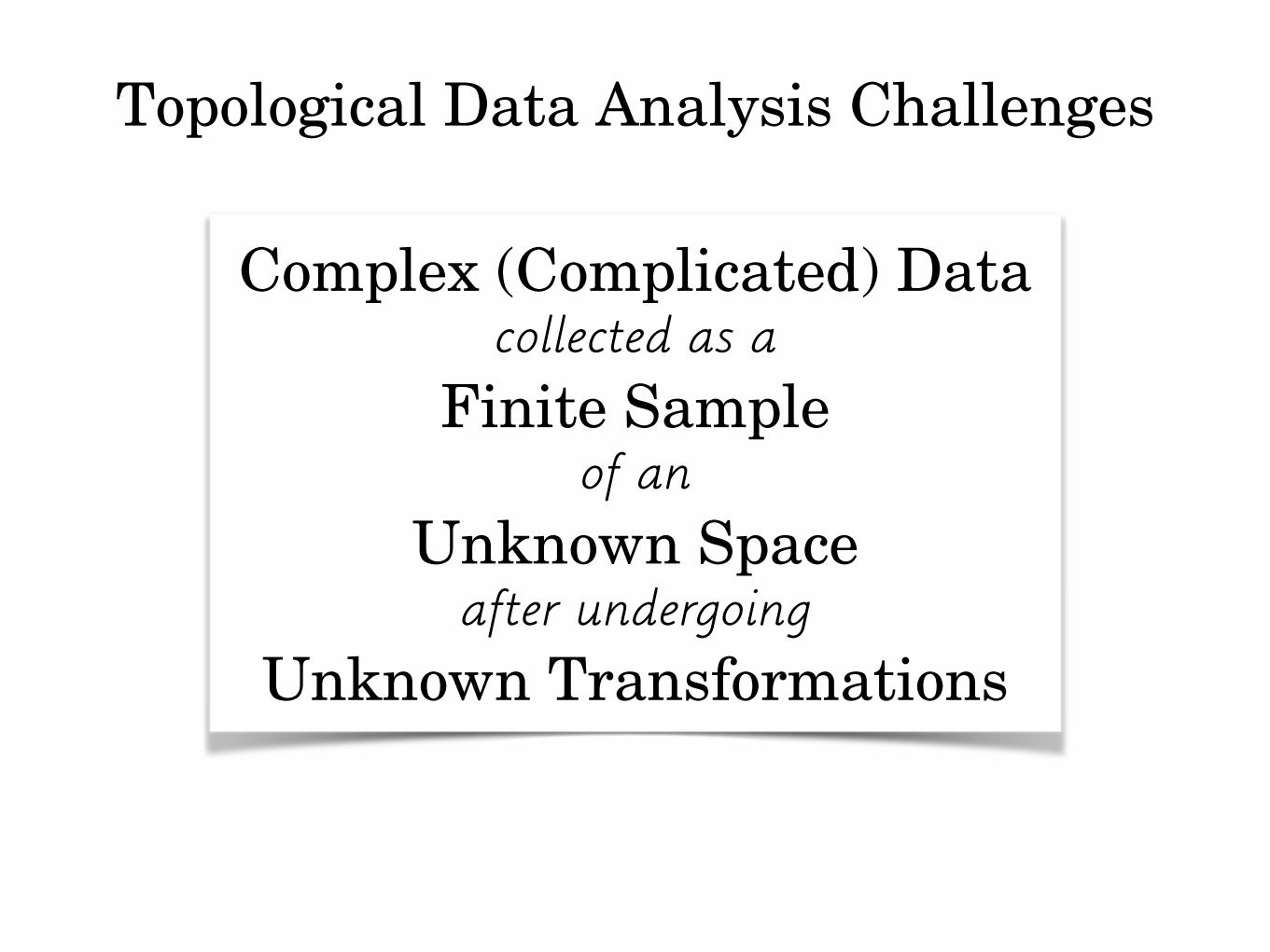
Topological Data Analysis Challenges

Topological Data Analysis Challenges
Complex (Complicated) Data

Topological Data Analysis Challenges
Complex (Complicated) Datacollected as a
Topological Data Analysis Challenges
Complex (Complicated) Datacollected as a
Finite Sample
Topological Data Analysis Challenges
Complex (Complicated) Datacollected as a
Finite Sampleof an

Topological Data Analysis Challenges
Complex (Complicated) Datacollected as a
Finite Sampleof an
Unknown Space
Topological Data Analysis Challenges
Complex (Complicated) Datacollected as a
Finite Sampleof an
Unknown Spaceafter undergoing
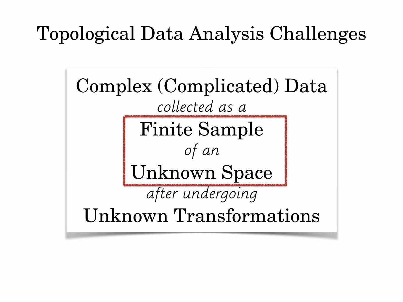
Topological Data Analysis Challenges
Complex (Complicated) Datacollected as a
Finite Sampleof an
Unknown Spaceafter undergoing
Unknown Transformations
Topological Data Analysis Challenges
Complex (Complicated) Datacollected as a
Finite Sampleof an
Unknown Spaceafter undergoing
Unknown Transformations

Unions of Balls
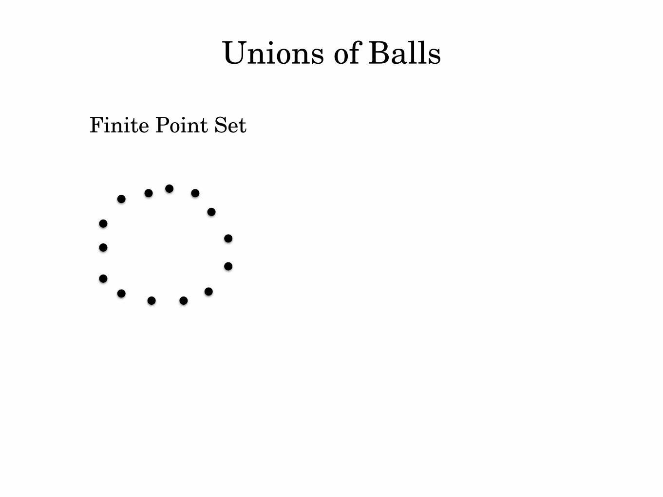
Unions of Balls
Finite Point Set
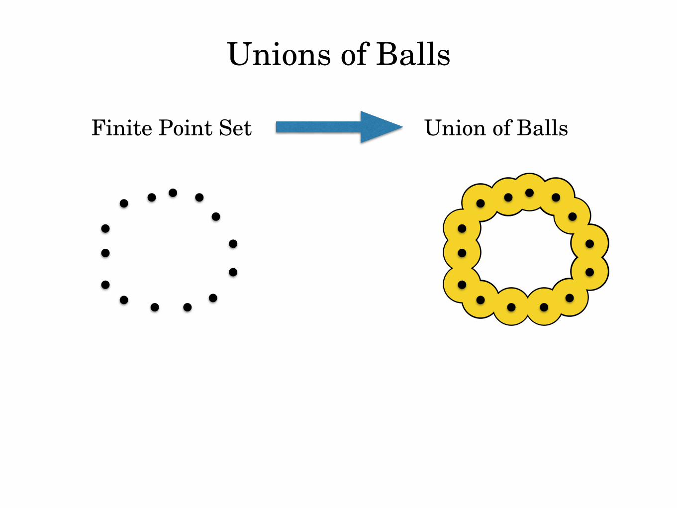
Unions of Balls
Finite Point Set Union of Balls
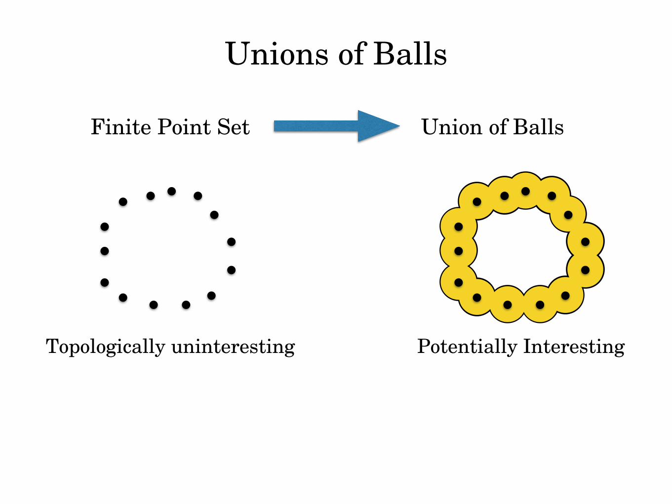
Unions of Balls
Finite Point Set Union of Balls
Topologically uninteresting Potentially Interesting
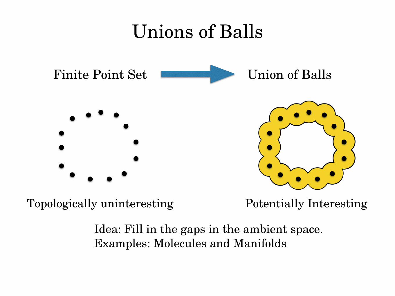
Unions of Balls
Finite Point Set Union of Balls
Topologically uninteresting Potentially Interesting
Idea: Fill in the gaps in the ambient space. Examples: Molecules and Manifolds
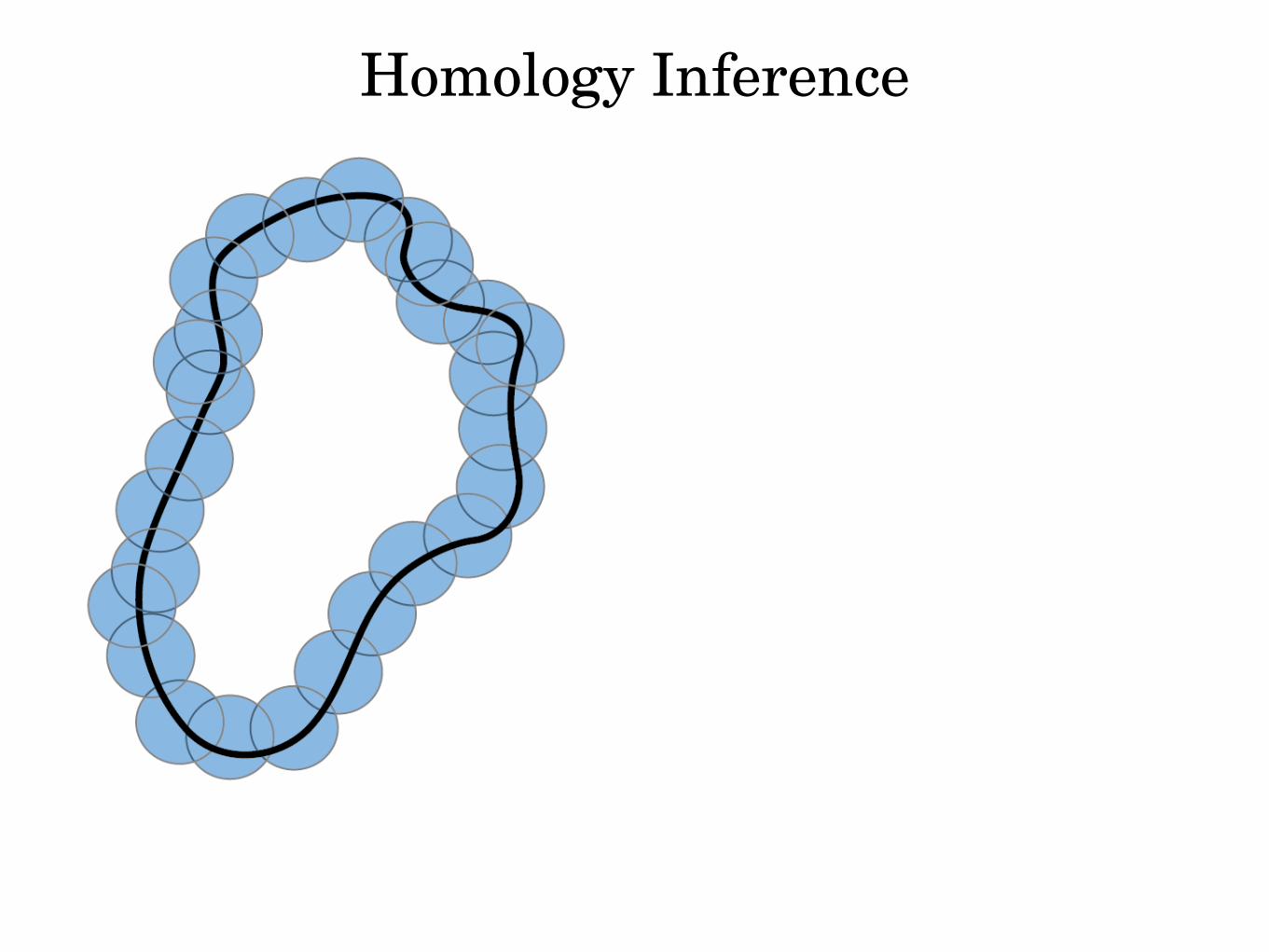
Homology Inference
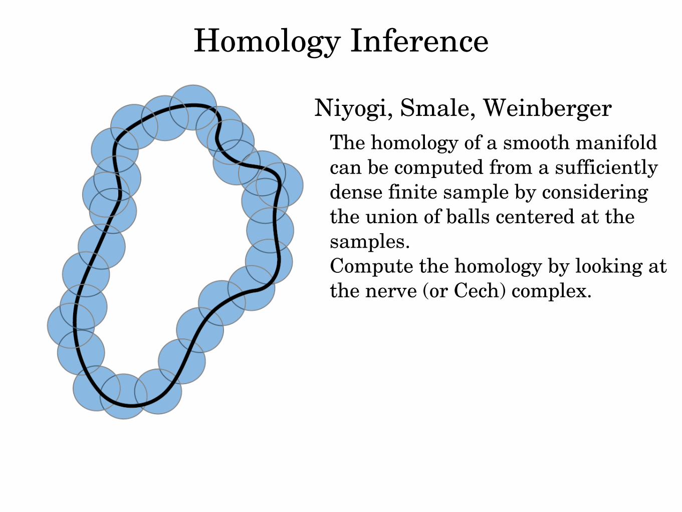
Homology Inference
Niyogi, Smale, WeinbergerThe homology of a smooth manifold can be computed from a sufficiently dense finite sample by considering the union of balls centered at the samples. Compute the homology by looking at the nerve (or Cech) complex.
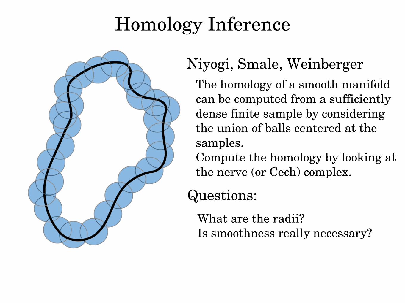
Homology Inference
Niyogi, Smale, WeinbergerThe homology of a smooth manifold can be computed from a sufficiently dense finite sample by considering the union of balls centered at the samples. Compute the homology by looking at the nerve (or Cech) complex.
Questions:
What are the radii? Is smoothness really necessary?
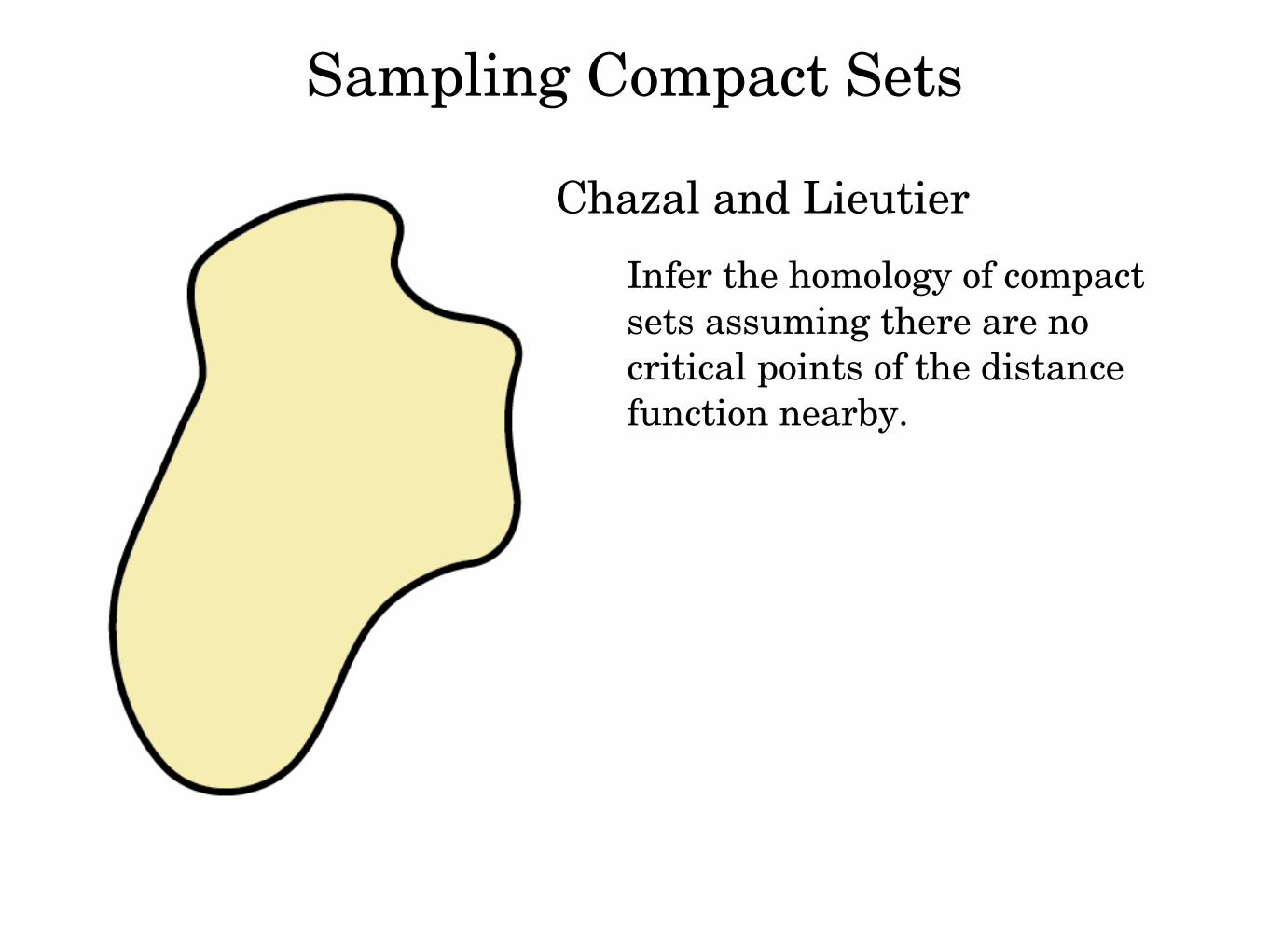
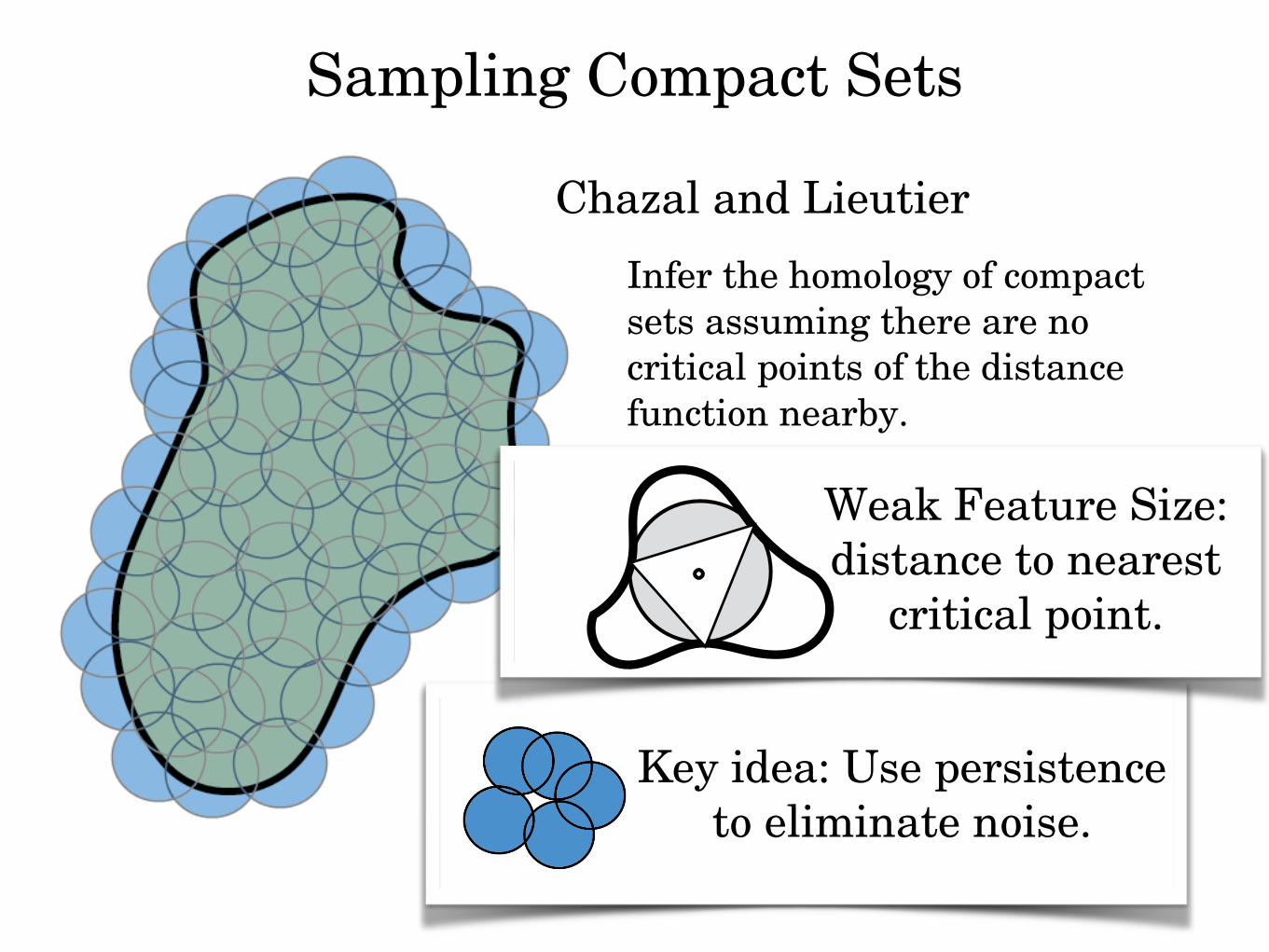
Sampling Compact Sets
Chazal and Lieutier
Infer the homology of compact sets assuming there are no critical points of the distance function nearby.
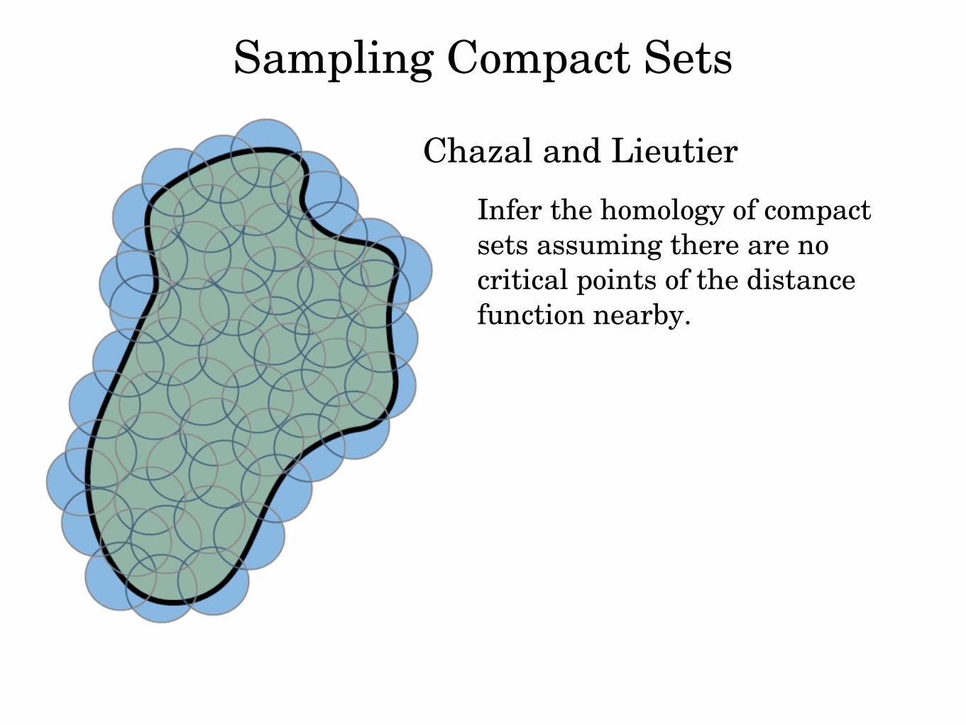
Sampling Compact Sets
Chazal and Lieutier
Infer the homology of compact sets assuming there are no critical points of the distance function nearby.
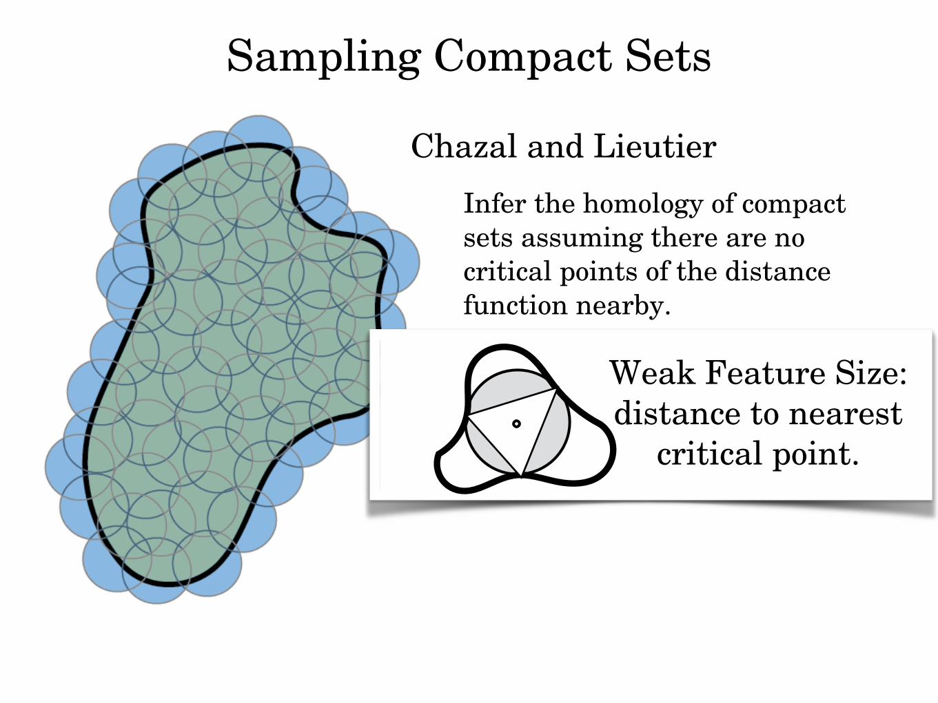
Sampling Compact Sets
Chazal and Lieutier
Infer the homology of compact sets assuming there are no critical points of the distance function nearby.
Weak Feature Size: distance to nearest
critical point.
Sampling Compact Sets
Key idea: Use persistence to eliminate noise.
Chazal and Lieutier
Infer the homology of compact sets assuming there are no critical points of the distance function nearby.
Weak Feature Size: distance to nearest
critical point.
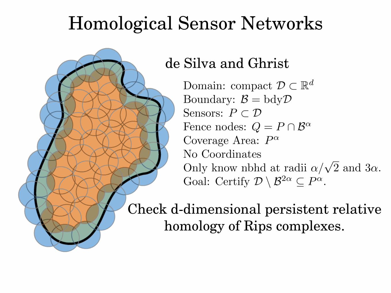
Homological Sensor Networks
Domain: compact D ⇢ Rd
Boundary: B = bdyDSensors: P ⇢ DFence nodes: Q = P \ B↵
Coverage Area: P↵
No CoordinatesOnly know nbhd at radii ↵/
p2 and 3↵.
Goal: Certify D \ B2↵ ✓ P↵.
de Silva and Ghrist
Check d-dimensional persistent relative homology of Rips complexes.
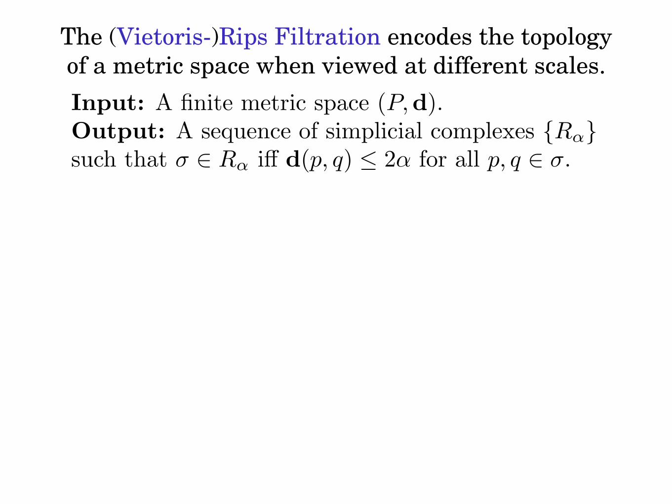
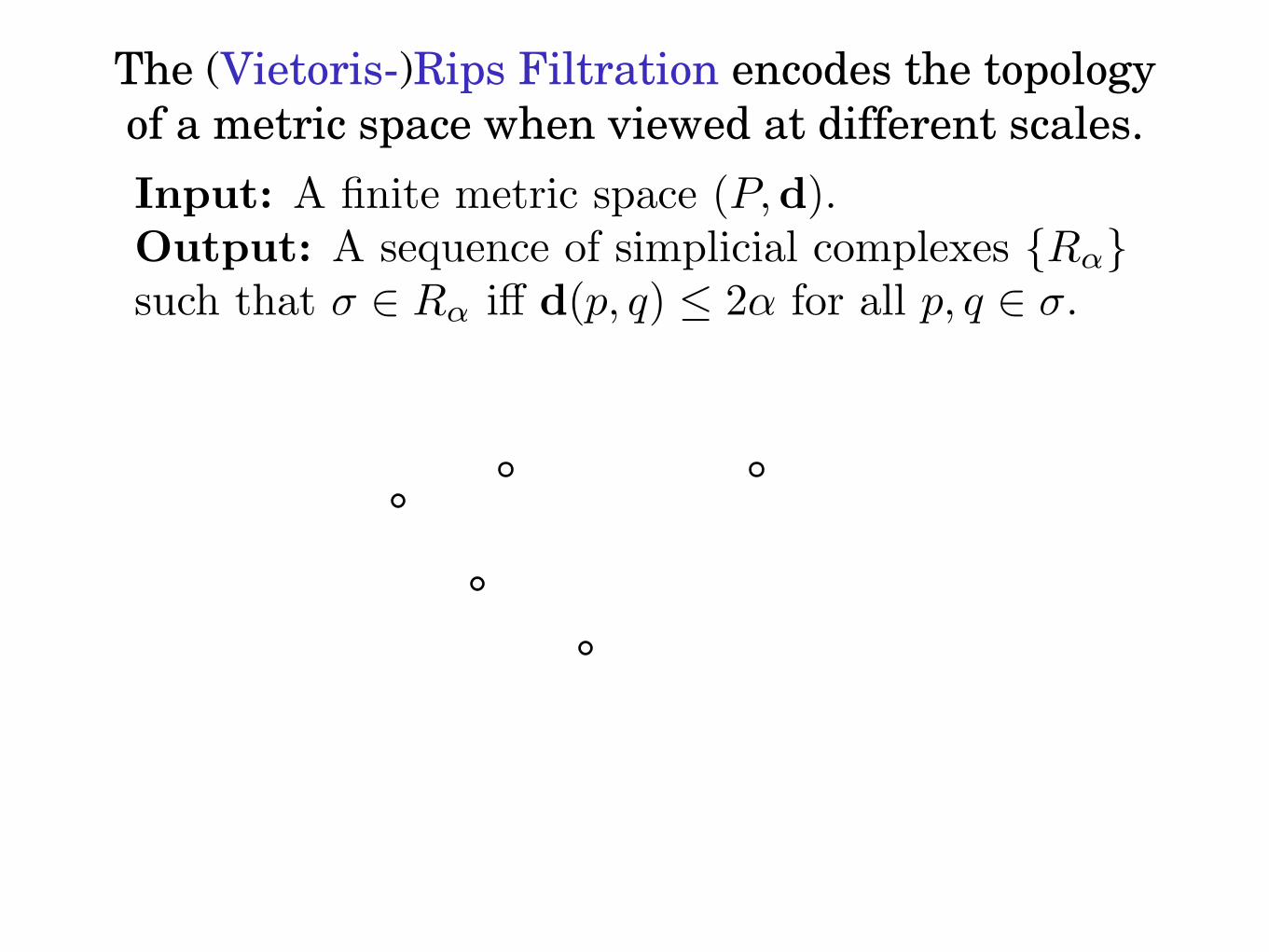
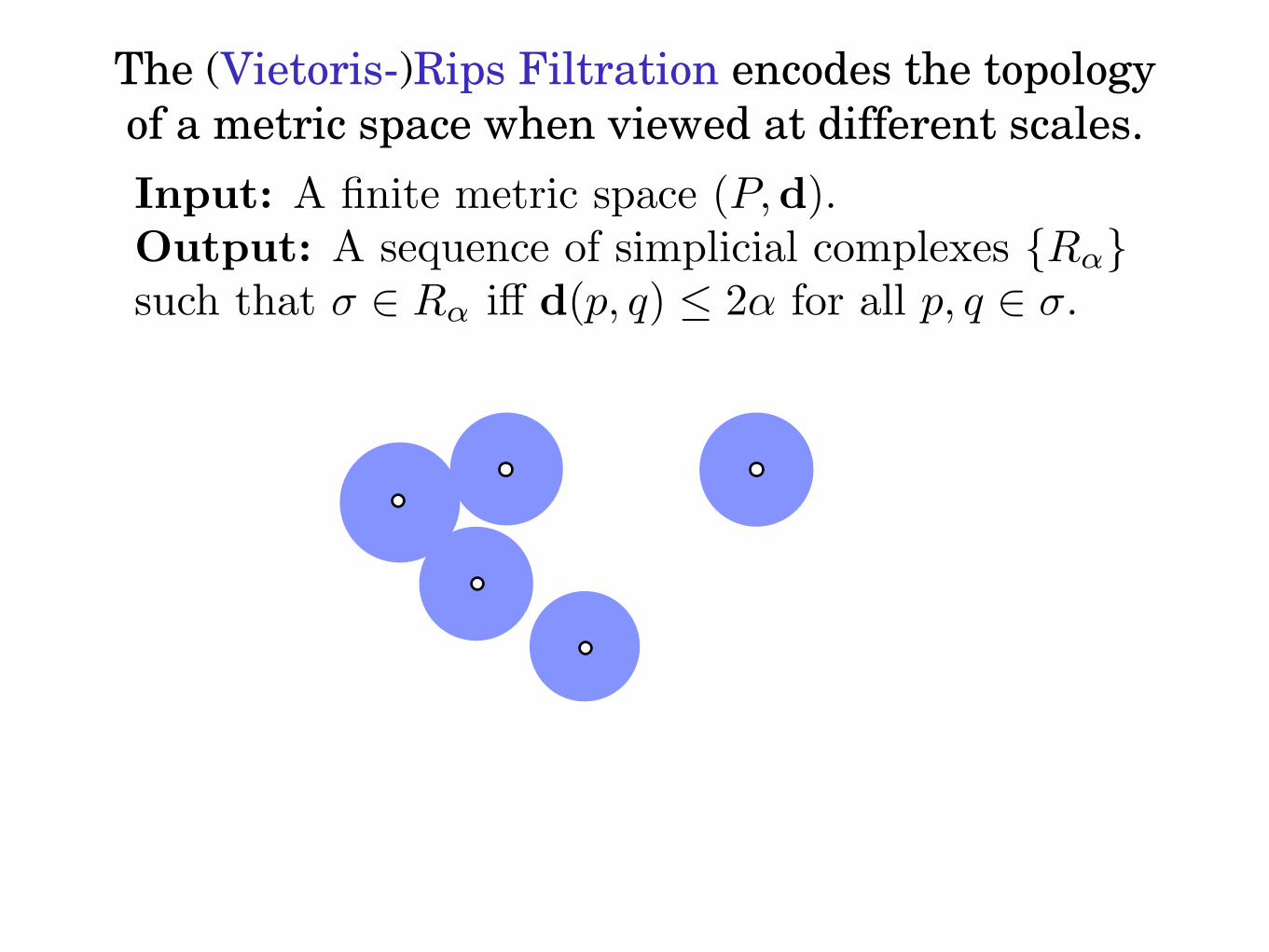
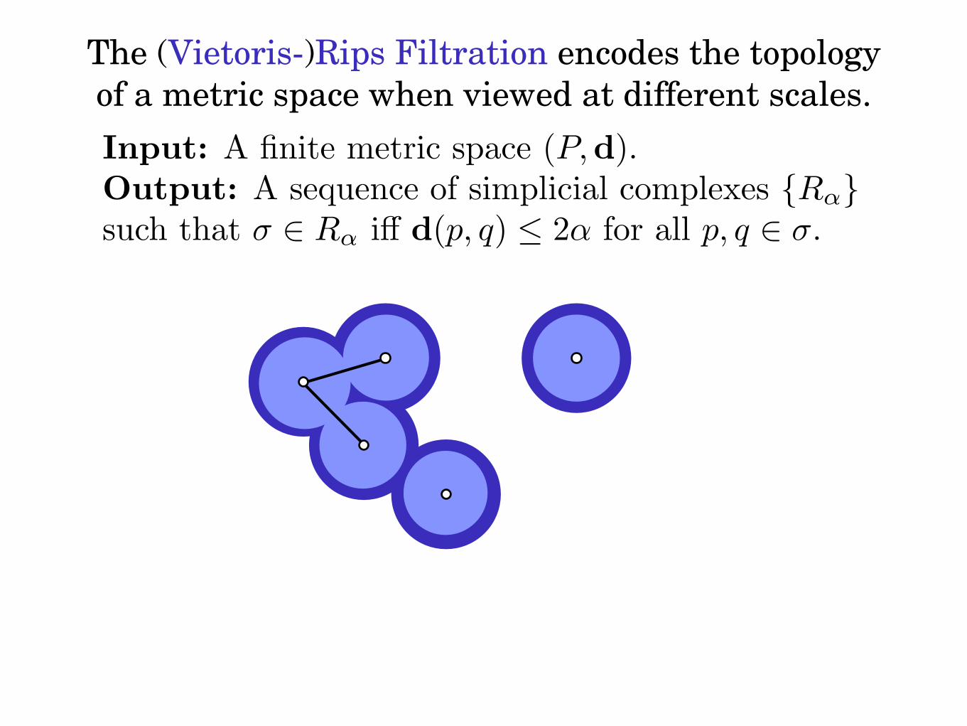
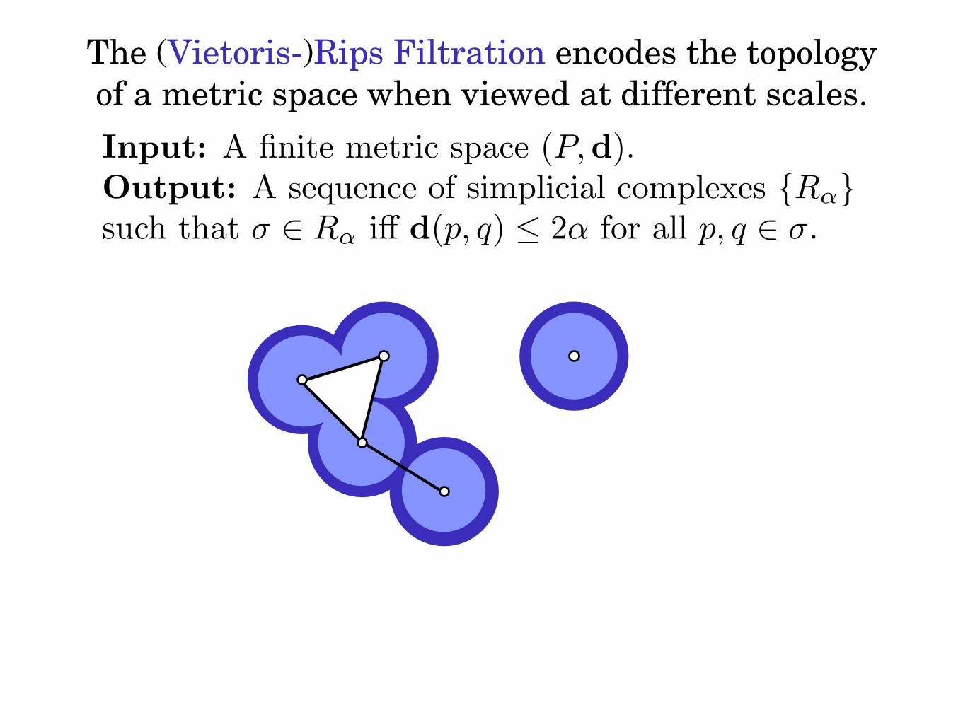
The (Vietoris-)Rips Filtration encodes the topology of a metric space when viewed at different scales.
Input: A finite metric space (P,d).Output: A sequence of simplicial complexes {Rα}such that σ ∈ Rα iff d(p, q) ≤ 2α for all p, q ∈ σ.
The (Vietoris-)Rips Filtration encodes the topology of a metric space when viewed at different scales.
Input: A finite metric space (P,d).Output: A sequence of simplicial complexes {Rα}such that σ ∈ Rα iff d(p, q) ≤ 2α for all p, q ∈ σ.
The (Vietoris-)Rips Filtration encodes the topology of a metric space when viewed at different scales.
Input: A finite metric space (P,d).Output: A sequence of simplicial complexes {Rα}such that σ ∈ Rα iff d(p, q) ≤ 2α for all p, q ∈ σ.

The (Vietoris-)Rips Filtration encodes the topology of a metric space when viewed at different scales.
Input: A finite metric space (P,d).Output: A sequence of simplicial complexes {Rα}such that σ ∈ Rα iff d(p, q) ≤ 2α for all p, q ∈ σ.
The (Vietoris-)Rips Filtration encodes the topology of a metric space when viewed at different scales.
Input: A finite metric space (P,d).Output: A sequence of simplicial complexes {Rα}such that σ ∈ Rα iff d(p, q) ≤ 2α for all p, q ∈ σ.
The (Vietoris-)Rips Filtration encodes the topology of a metric space when viewed at different scales.
Input: A finite metric space (P,d).Output: A sequence of simplicial complexes {Rα}such that σ ∈ Rα iff d(p, q) ≤ 2α for all p, q ∈ σ.
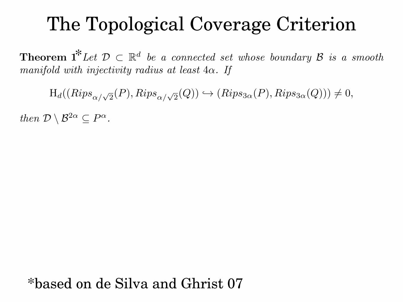
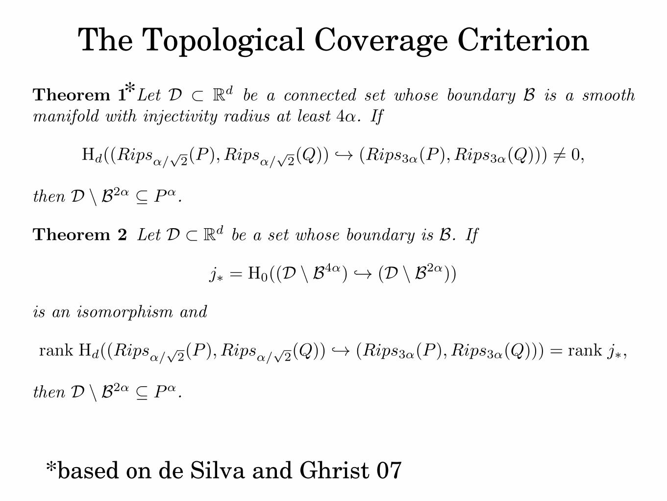
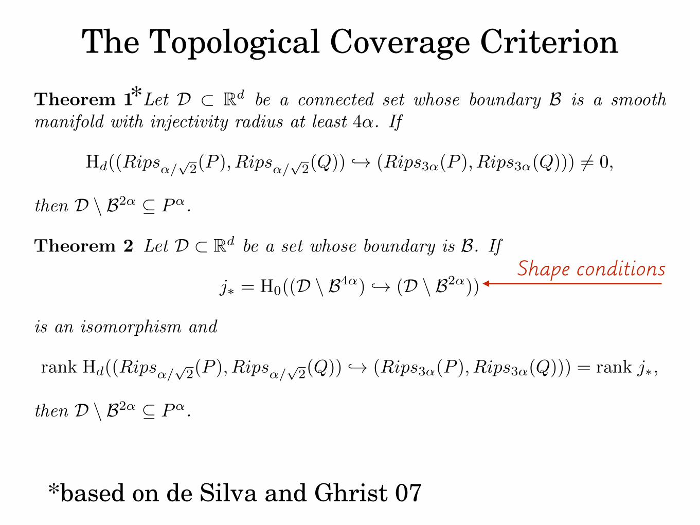
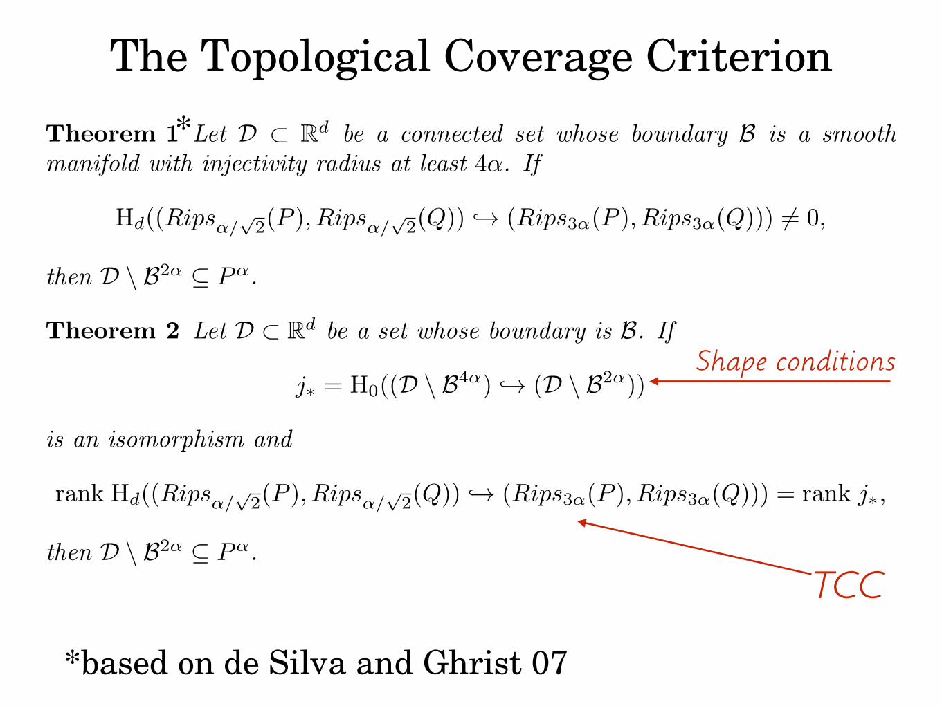
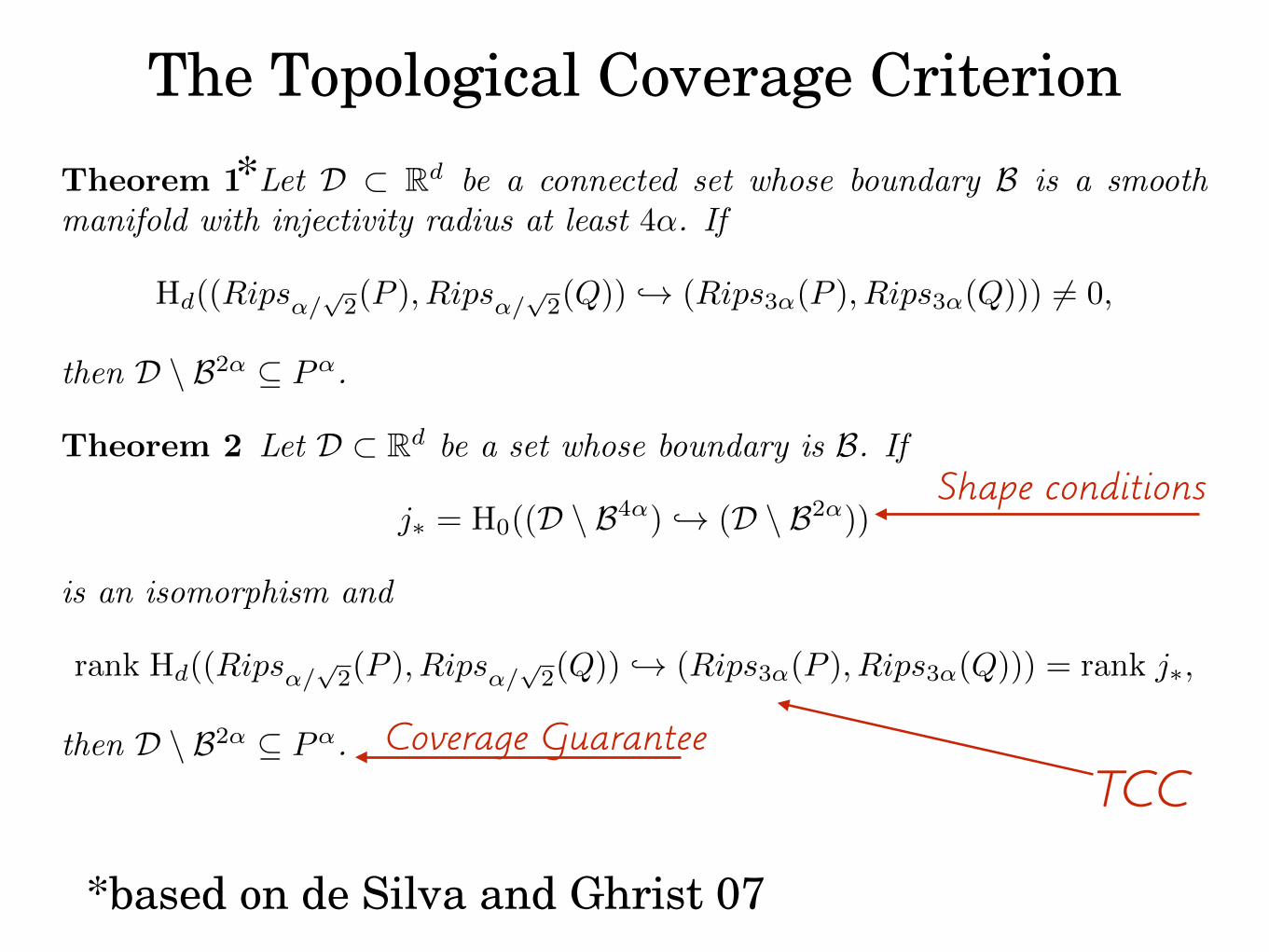
The Topological Coverage Criterion
*based on de Silva and Ghrist 07
Theorem 1 Let D ⇢ Rdbe a connected set whose boundary B is a smooth
manifold with injectivity radius at least 4↵. If
Hd((Rips↵/p2(P ), Rips↵/
p2(Q)) ,! (Rips3↵(P ), Rips3↵(Q))) 6= 0,
then D \ B2↵ ✓ P↵.
Theorem 2 Let D ⇢ Rdbe a set whose boundary is B. If
j⇤ = H0((D \ B4↵) ,! (D \ B2↵))
is an isomorphism and
rank Hd((Rips↵/p2(P ), Rips↵/
p2(Q)) ,! (Rips3↵(P ), Rips3↵(Q))) = rank j⇤,
then D \ B2↵ ✓ P↵.
*
Shape conditions
TCC
The Topological Coverage Criterion
*based on de Silva and Ghrist 07
Theorem 1 Let D ⇢ Rdbe a connected set whose boundary B is a smooth
manifold with injectivity radius at least 4↵. If
Hd((Rips↵/p2(P ), Rips↵/
p2(Q)) ,! (Rips3↵(P ), Rips3↵(Q))) 6= 0,
then D \ B2↵ ✓ P↵.
Theorem 2 Let D ⇢ Rdbe a set whose boundary is B. If
j⇤ = H0((D \ B4↵) ,! (D \ B2↵))
is an isomorphism and
rank Hd((Rips↵/p2(P ), Rips↵/
p2(Q)) ,! (Rips3↵(P ), Rips3↵(Q))) = rank j⇤,
then D \ B2↵ ✓ P↵.
*
Shape conditions
TCCCoverage Guarantee
Key tricks
Key tricks
1 Alexander Duality - coverage to connectivity
Key tricks
1 Alexander Duality - coverage to connectivity
2 The Nerve Theorem - discretize the geoemtry
Key tricks
1 Alexander Duality - coverage to connectivity
2 The Nerve Theorem - discretize the geoemtry
3 Rips-Cech Interleaving - work without coordinates
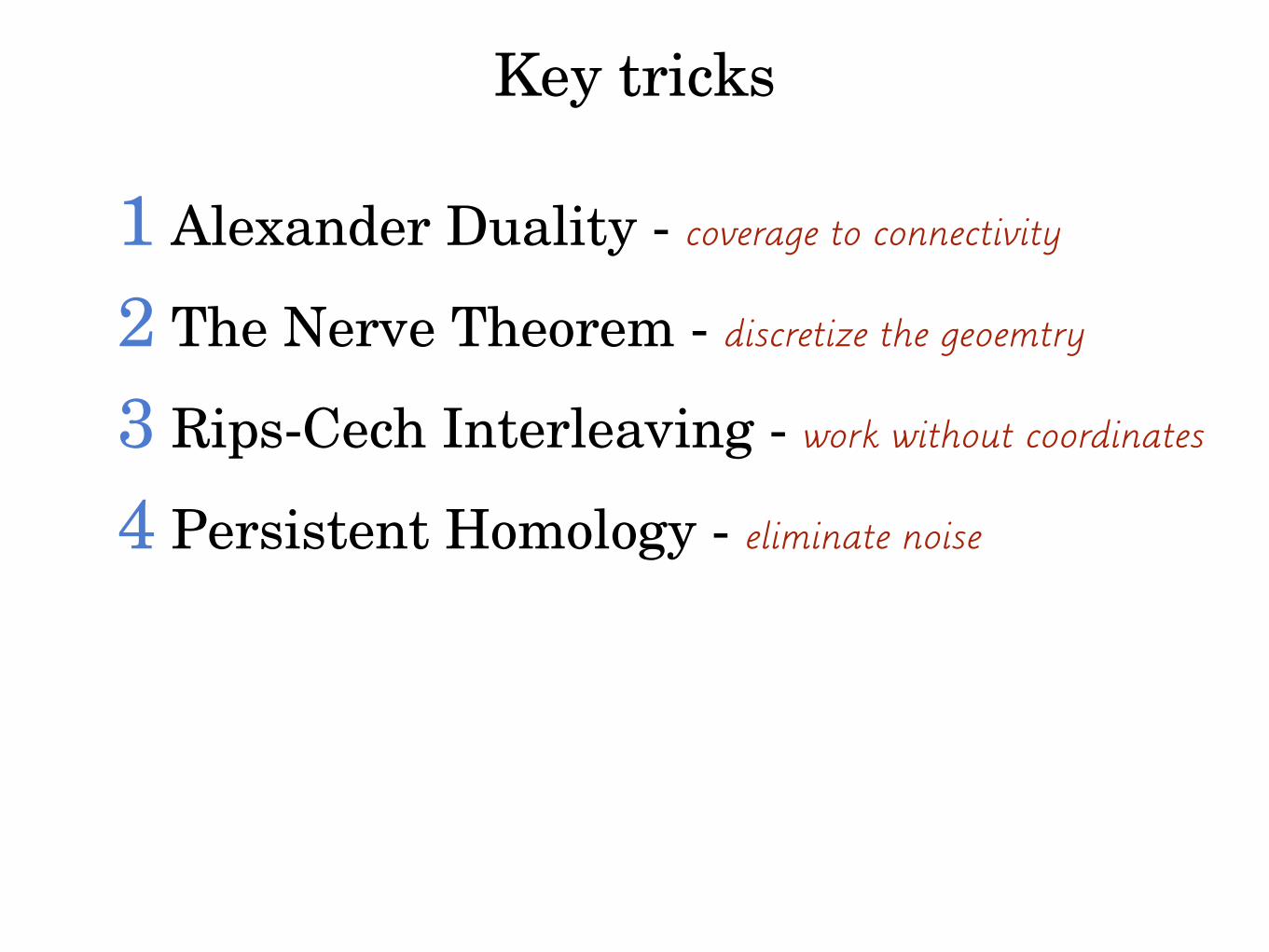
Key tricks
1 Alexander Duality - coverage to connectivity
2 The Nerve Theorem - discretize the geoemtry
3 Rips-Cech Interleaving - work without coordinates
4 Persistent Homology - eliminate noise

Tricks: Alexander Duality

Tricks: Alexander DualityHd(D,B) ⇠= H0(B, D)

Tricks: Alexander DualityHd(D,B) ⇠= H0(B, D) ⇠= H0(D \ B)
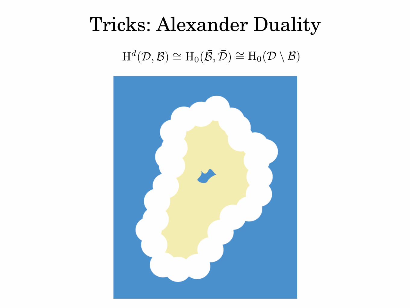
Tricks: Alexander DualityHd(D,B) ⇠= H0(B, D) ⇠= H0(D \ B)
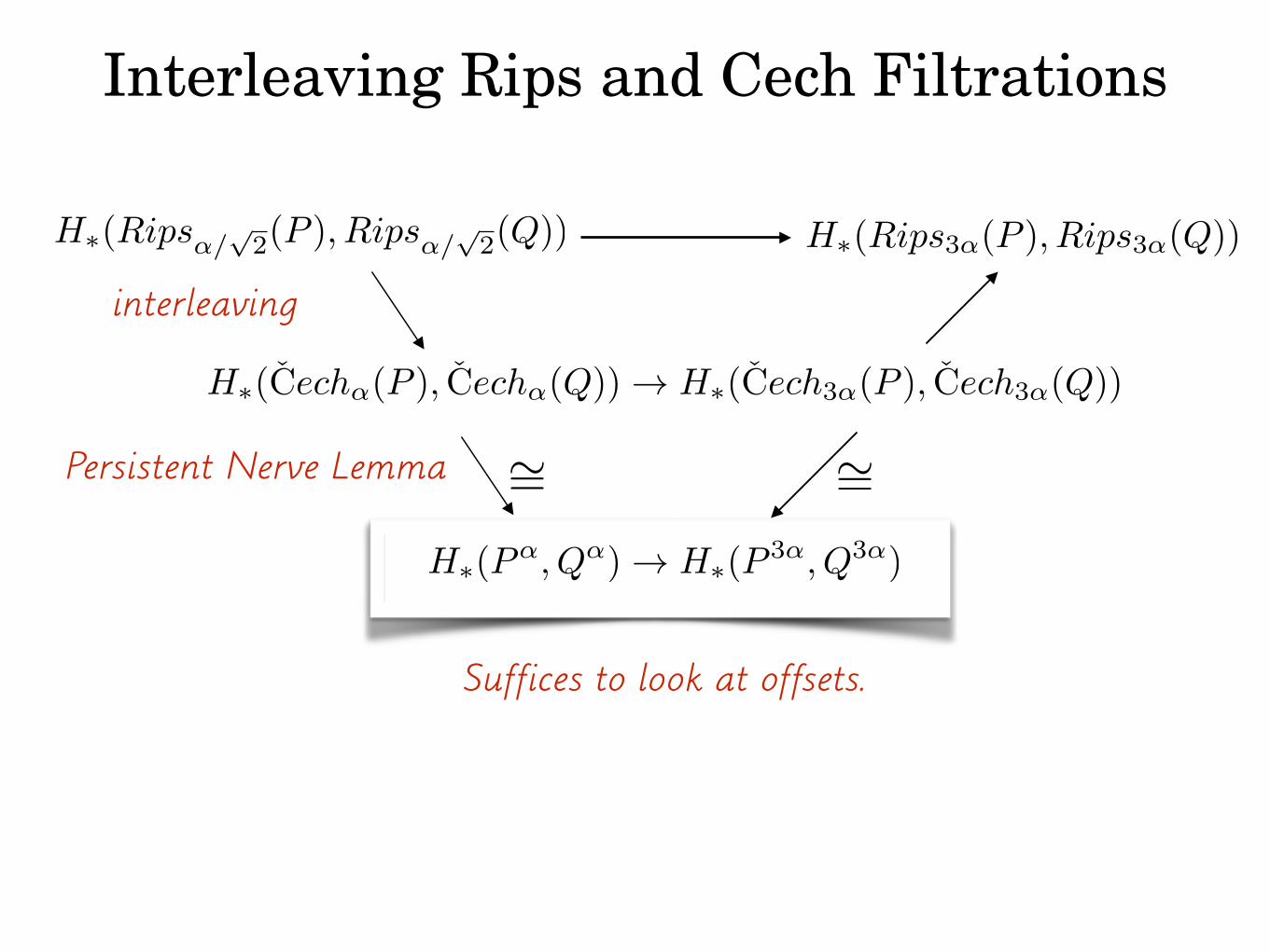
Interleaving Rips and Cech Filtrations
H⇤(Rips↵/p2(P ), Rips↵/
p2(Q)) H⇤(Rips3↵(P ), Rips3↵(Q))
H⇤(Cech↵(P ), Cech↵(Q)) ! H⇤(Cech3↵(P ), Cech3↵(Q))
H⇤(P↵, Q↵) ! H⇤(P
3↵, Q3↵)
⇠=⇠=
interleaving
Persistent Nerve Lemma
Suffices to look at offsets.
Tricks: Persistent Homology
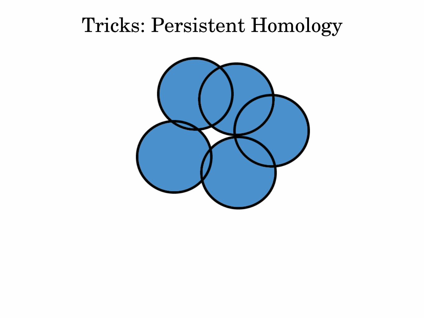
Tricks: Persistent Homology
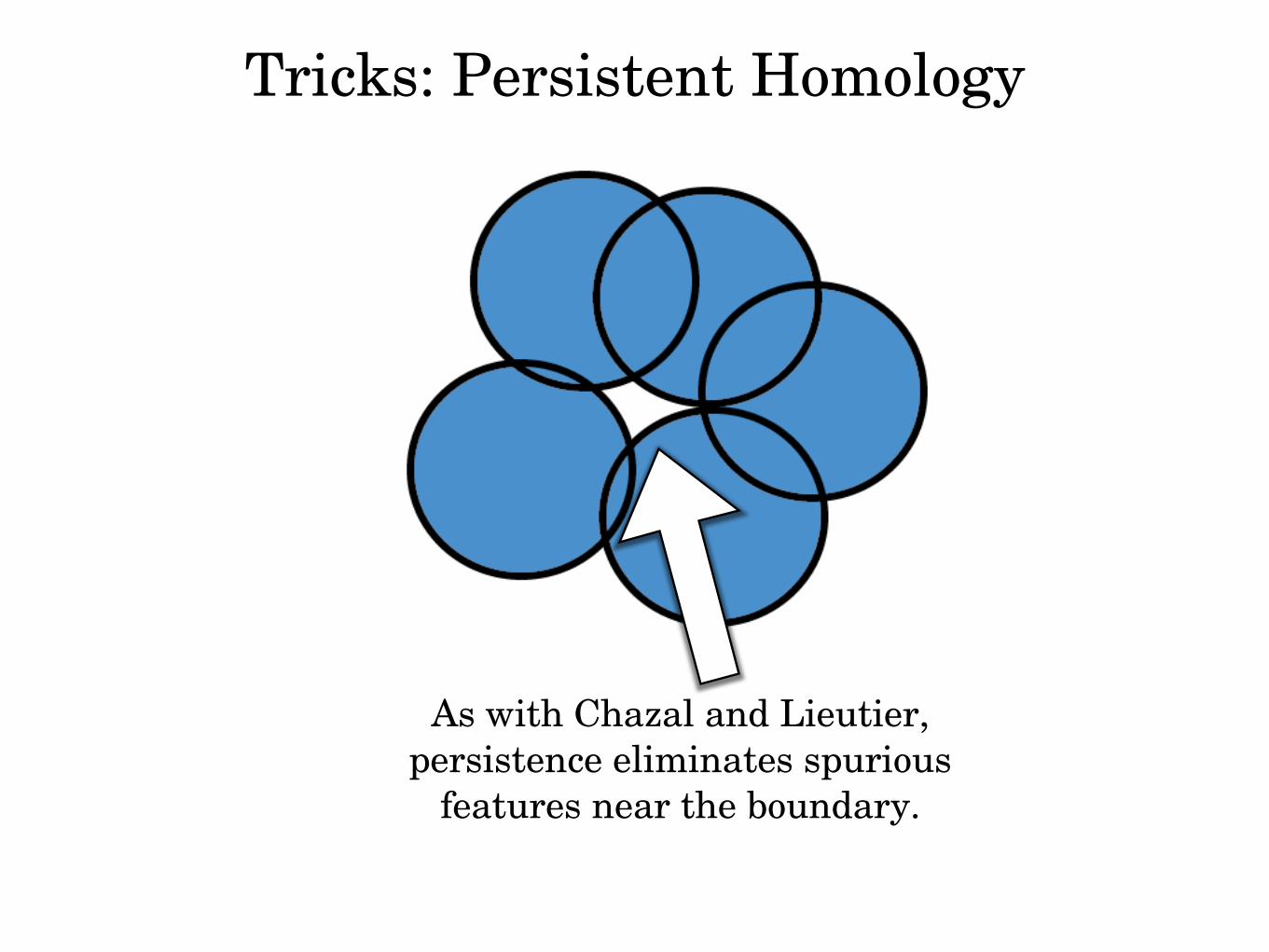
Tricks: Persistent Homology
As with Chazal and Lieutier, persistence eliminates spurious
features near the boundary.

TCC Proof Idea I

TCC Proof Idea I
P↵ ,! D2↵

TCC Proof Idea I
P↵ ,! D2↵
(P↵, Q↵) ,! (D2↵,B2↵)

TCC Proof Idea I
P↵ ,! D2↵
(P↵, Q↵) ,! (D2↵,B2↵)
Hd(D2↵,B2↵) ! Hd(P↵, Q↵)

TCC Proof Idea I
P↵ ,! D2↵
(P↵, Q↵) ,! (D2↵,B2↵)
surjectivity implies coverage
Hd(D2↵,B2↵) ! Hd(P↵, Q↵)

TCC Proof Idea I
P↵ ,! D2↵
(P↵, Q↵) ,! (D2↵,B2↵)
surjectivity implies coverage
a⇤ : H0(B2↵,D2↵) ! H0(Q↵, P↵)
Hd(D2↵,B2↵) ! Hd(P↵, Q↵)

TCC Proof Idea I
P↵ ,! D2↵
(P↵, Q↵) ,! (D2↵,B2↵)
surjectivity implies coverage
a⇤ : H0(B2↵,D2↵) ! H0(Q↵, P↵)
a* injective implies “coverage”, i.e. (D \ B2↵ ✓ P↵)
Hd(D2↵,B2↵) ! Hd(P↵, Q↵)
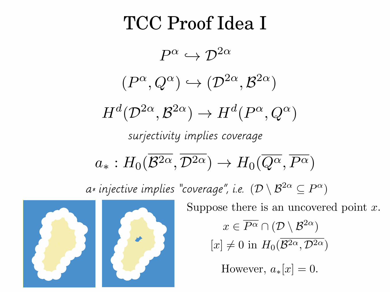
TCC Proof Idea I
P↵ ,! D2↵
(P↵, Q↵) ,! (D2↵,B2↵)
surjectivity implies coverage
a⇤ : H0(B2↵,D2↵) ! H0(Q↵, P↵)
a* injective implies “coverage”, i.e. (D \ B2↵ ✓ P↵)
[x] 6= 0 in H0(B2↵,D2↵)
Suppose there is an uncovered point x.
However, a⇤[x] = 0.
x 2 P
↵ \ (D \ B2↵)
Hd(D2↵,B2↵) ! Hd(P↵, Q↵)

TCC Proof Idea IIa⇤ : H0(B2↵,D2↵) ! H0(Q↵, P↵)
a* injective implies “coverage”, i.e. (D \ B2↵ ✓ P↵)

TCC Proof Idea IIa⇤ : H0(B2↵,D2↵) ! H0(Q↵, P↵)
a* injective implies “coverage”, i.e. (D \ B2↵ ✓ P↵)
If D \B2↵is connected and a⇤ is surjective,
then we can infer coverage by computing H0(Q↵, P↵).

TCC Proof Idea IIa⇤ : H0(B2↵,D2↵) ! H0(Q↵, P↵)
a* injective implies “coverage”, i.e. (D \ B2↵ ✓ P↵)
If D \B2↵is connected and a⇤ is surjective,
then we can infer coverage by computing H0(Q↵, P↵).
Problem: There could be “spurious” features.
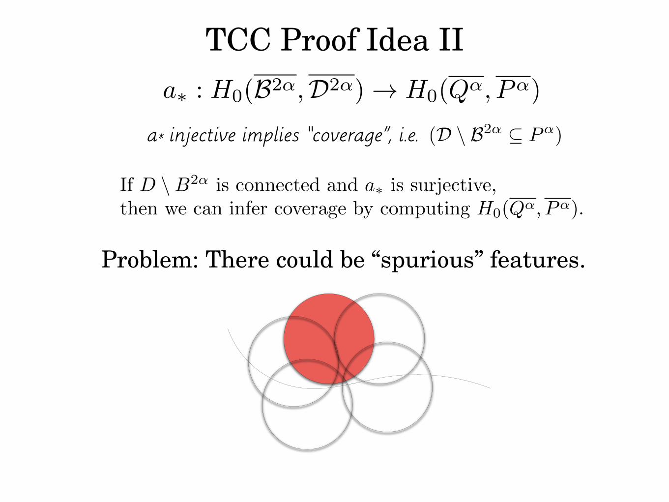
TCC Proof Idea IIa⇤ : H0(B2↵,D2↵) ! H0(Q↵, P↵)
a* injective implies “coverage”, i.e. (D \ B2↵ ✓ P↵)
If D \B2↵is connected and a⇤ is surjective,
then we can infer coverage by computing H0(Q↵, P↵).
Problem: There could be “spurious” features.
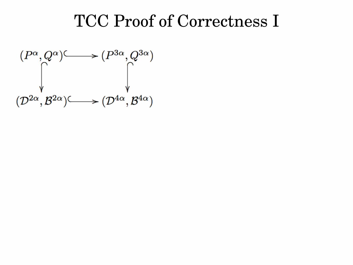
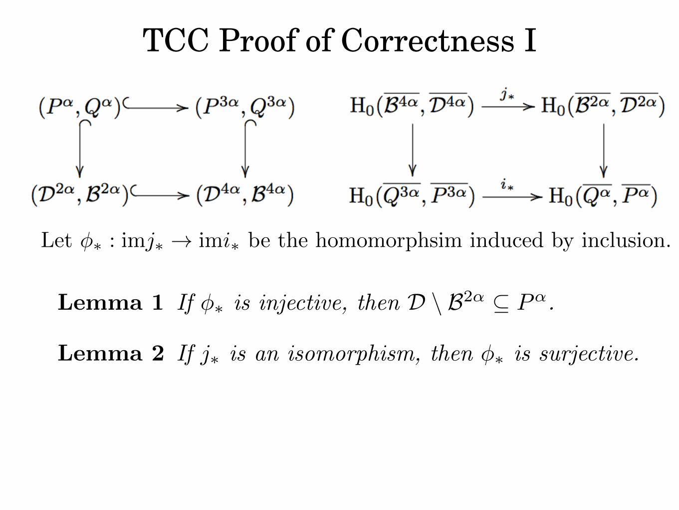
TCC Proof of Correctness I
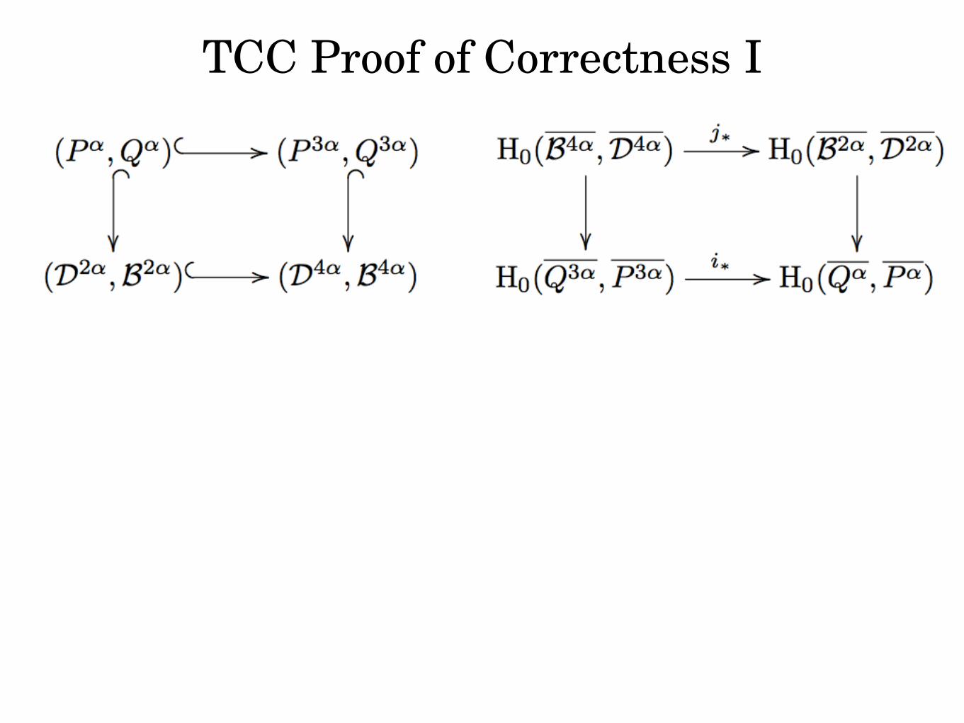
TCC Proof of Correctness I
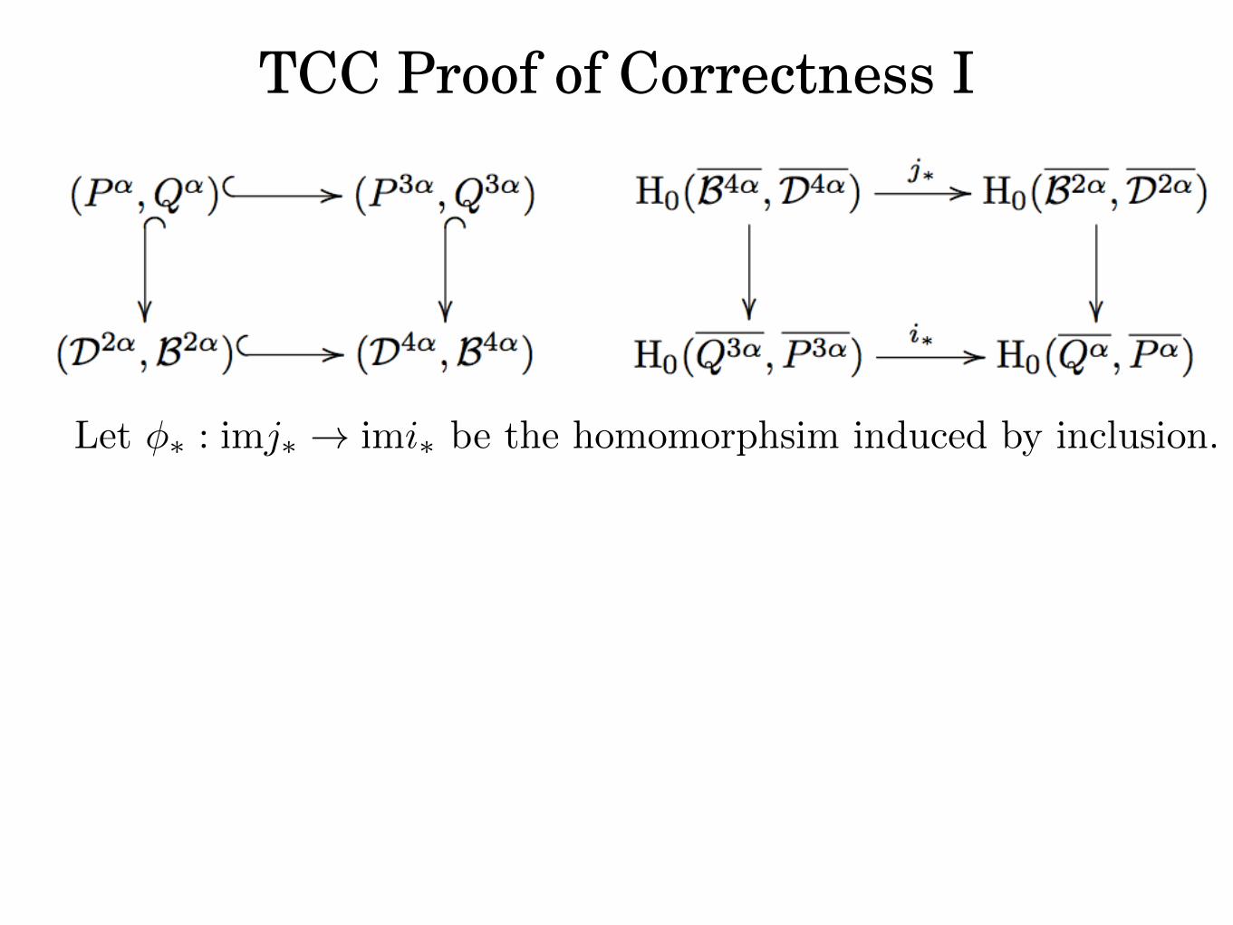
TCC Proof of Correctness I
Let �⇤ : imj⇤ ! imi⇤ be the homomorphsim induced by inclusion.
TCC Proof of Correctness I
Let �⇤ : imj⇤ ! imi⇤ be the homomorphsim induced by inclusion.
Lemma 1 If �⇤ is injective, then D \ B2↵ ✓ P↵.
Lemma 2 If j⇤ is an isomorphism, then �⇤ is surjective.
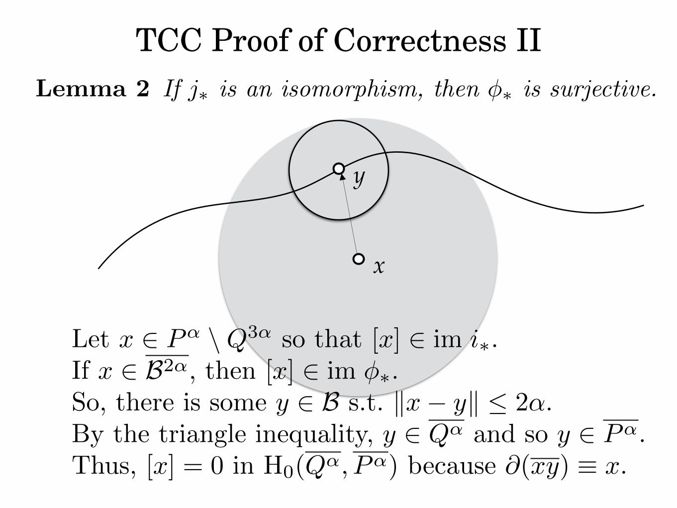
TCC Proof of Correctness IILemma 2 If j⇤ is an isomorphism, then �⇤ is surjective.
x
y
Let x 2 P
↵ \Q3↵ so that [x] 2 im i⇤.If x 2 B2↵, then [x] 2 im �⇤.So, there is some y 2 B s.t. kx� yk 2↵.By the triangle inequality, y 2 Q
↵ and so y 2 P
↵.Thus, [x] = 0 in H0(Q↵
, P
↵) because @(xy) ⌘ x.
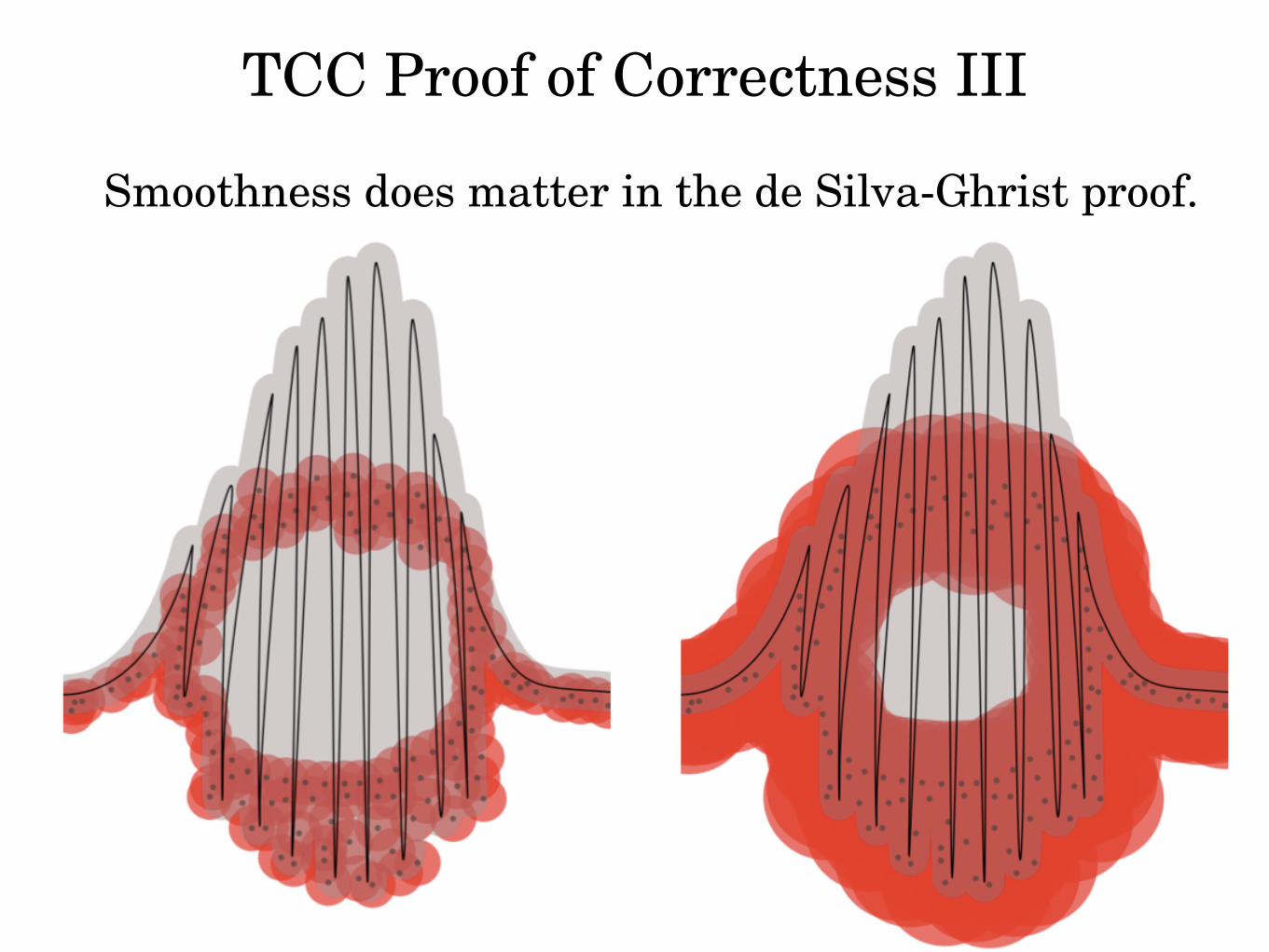
TCC Proof of Correctness III
Smoothness does matter in the de Silva-Ghrist proof.
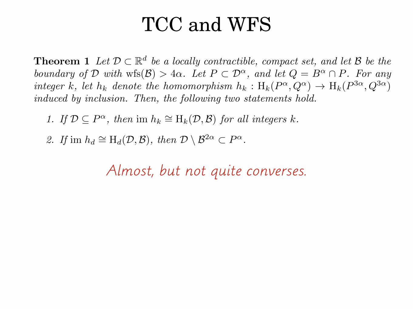
TCC and WFS
Theorem 1 Let D ⇢ Rdbe a locally contractible, compact set, and let B be the
boundary of D with wfs(B) > 4↵. Let P ⇢ D↵, and let Q = B↵ \ P . For any
integer k, let hk denote the homomorphism hk : Hk(P↵, Q↵) ! Hk(P 3↵, Q3↵)induced by inclusion. Then, the following two statements hold.
1. If D ✓ P↵, then im hk
⇠= Hk(D,B) for all integers k.
2. If im hd⇠= Hd(D,B), then D \ B2↵ ⇢ P↵
.
Almost, but not quite converses.
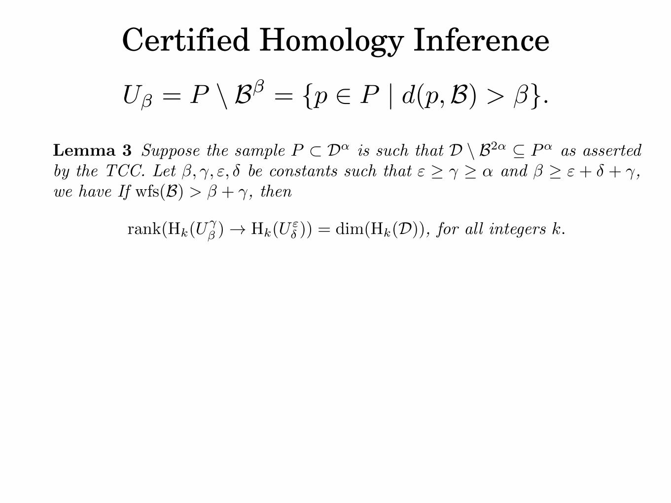
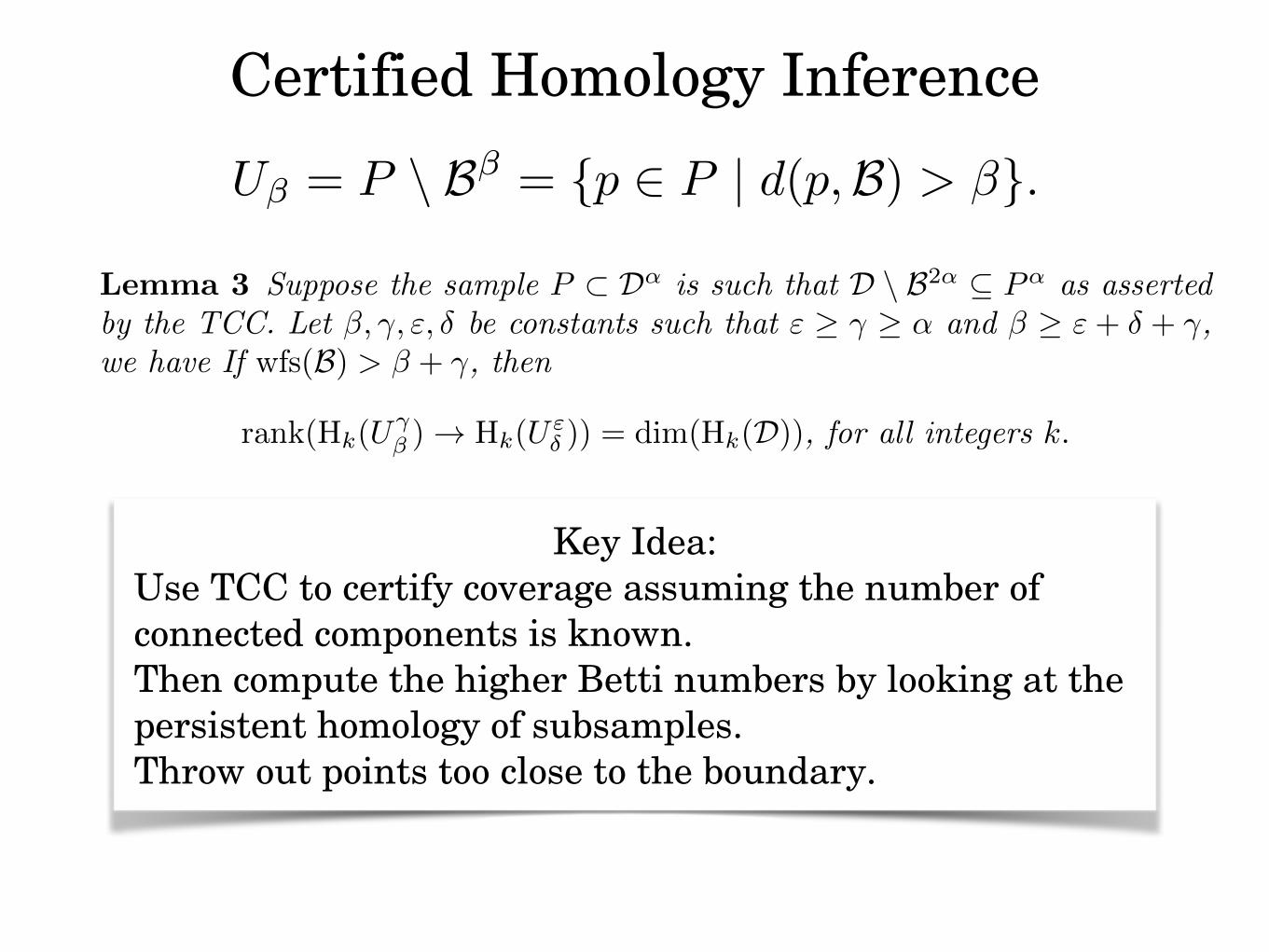
Certified Homology Inference
U� = P \ B� = {p 2 P | d(p,B) > �}.
Lemma 3 Suppose the sample P ⇢ D↵is such that D \ B2↵ ✓ P↵
as asserted
by the TCC. Let �, �, ", � be constants such that " � � � ↵ and � � "+ � + �,we have If wfs(B) > � + �, then
rank(Hk(U�� ) ! Hk(U
"� )) = dim(Hk(D)), for all integers k.
Key Idea: Use TCC to certify coverage assuming the number of connected components is known. Then compute the higher Betti numbers by looking at the persistent homology of subsamples. Throw out points too close to the boundary.

k-CoverageLemma 2 If j⇤ is an isomorphism, then �⇤ is surjective.
x
y
Let x 2 P
↵k \Q3↵
k so that [x] 2 im i⇤.
If x 2 B2↵, then [x] 2 im �⇤.So, there is some y 2 B s.t. kx� yk 2↵.By the triangle inequality, y 2 Q
↵k and so y 2 P
↵k .
Thus, [x] = 0 in H0(Q↵k , P
↵k ) because @(xy) ⌘ x.
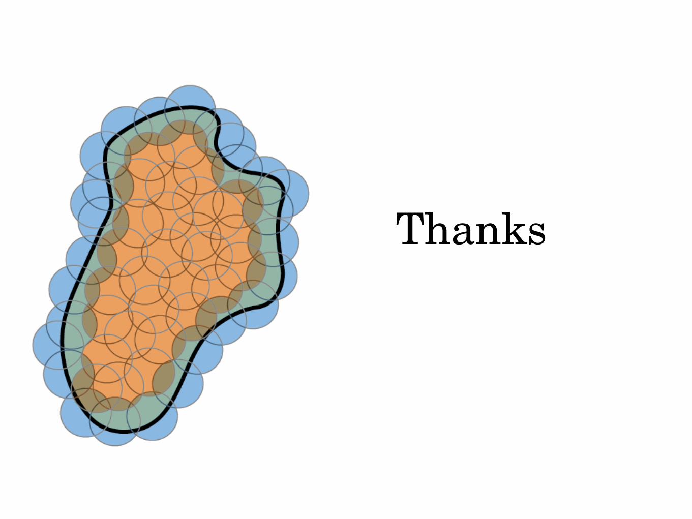
Thanks


![Brane Tilings and Homological Mirror Symmetrymember.ipmu.jp/masahito.yamazaki/files/2006/TIT2006.pdf · Partial Answer: Homological Mirror Symmetry [Kontsevich]: Db (cohY) | { z}](https://img.pdfslide.us/doc/110x75/5fac0c0bfbcb9f06ae38edb9/brane-tilings-and-homological-mirror-partial-answer-homological-mirror-symmetry.jpg)