Embed Size (px)
Citation preview
Advances in Mathematics 220 (2009) 1549–1601www.elsevier.com/locate/aim
Homological algebra for affine Hecke algebras
Eric Opdam, Maarten Solleveld ∗
Korteweg–de Vries Institute for Mathematics, Universiteit van Amsterdam, Plantage Muidergracht 24,1018TV Amsterdam, The Netherlands
Received 11 September 2007; accepted 4 November 2008
Available online 2 December 2008
Communicated by David Ben-Zvi
Abstract
In this paper we study homological properties of modules over an affine Hecke algebra H. In particularwe prove a comparison result for higher extensions of tempered modules when passing to the Schwartzalgebra S , a certain topological completion of the affine Hecke algebra. The proof is self-contained andbased on a direct construction of a bounded contraction of certain standard resolutions of H-modules.
This construction applies for all positive parameters of the affine Hecke algebra. This is an importantfeature, since it is an ingredient to analyse how the irreducible discrete series representations of H arise ingeneric families over the parameter space of H. For irreducible non-simply laced affine Hecke algebras thiswill enable us to give a complete classification of the discrete series characters, for all positive parameters(we will report on this application in a separate article).© 2008 Elsevier Inc. All rights reserved.
MSC: 20C08; 18Gxx; 20F55
Keywords: Homological algebra; Hecke algebras; Coxeter groups
Contents
0. Introduction . . . . . . . . . . . . . . . . . . . . . . . . . . . . . . . . . . . . . . . . . . . . . . . . . . . . . . . 15501. Preliminaries . . . . . . . . . . . . . . . . . . . . . . . . . . . . . . . . . . . . . . . . . . . . . . . . . . . . . . . 1553
1.1. Root data . . . . . . . . . . . . . . . . . . . . . . . . . . . . . . . . . . . . . . . . . . . . . . . . . . . . 15531.2. Affine Hecke algebras . . . . . . . . . . . . . . . . . . . . . . . . . . . . . . . . . . . . . . . . . . . . 1557
* Corresponding author.E-mail addresses: [email protected] (E. Opdam), [email protected] (M. Solleveld).
0001-8708/$ – see front matter © 2008 Elsevier Inc. All rights reserved.doi:10.1016/j.aim.2008.11.002
1550 E. Opdam, M. Solleveld / Advances in Mathematics 220 (2009) 1549–1601
1.3. The Schwartz completion . . . . . . . . . . . . . . . . . . . . . . . . . . . . . . . . . . . . . . . . . 15612. Projective resolutions . . . . . . . . . . . . . . . . . . . . . . . . . . . . . . . . . . . . . . . . . . . . . . . . . 1564
2.1. The bounded contraction of the polysimplicial complex . . . . . . . . . . . . . . . . . . . . . 15642.2. Projective resolutions for affine Hecke algebras . . . . . . . . . . . . . . . . . . . . . . . . . . . 15702.3. Projective resolutions for Schwartz algebras . . . . . . . . . . . . . . . . . . . . . . . . . . . . . 15752.4. Isocohomological inclusions . . . . . . . . . . . . . . . . . . . . . . . . . . . . . . . . . . . . . . . 1579
3. The Euler–Poincaré characteristic . . . . . . . . . . . . . . . . . . . . . . . . . . . . . . . . . . . . . . . . . 15823.1. Elliptic representation theory . . . . . . . . . . . . . . . . . . . . . . . . . . . . . . . . . . . . . . . 15823.2. The elliptic measure . . . . . . . . . . . . . . . . . . . . . . . . . . . . . . . . . . . . . . . . . . . . . 15863.3. Example: the Weyl group of type B2 . . . . . . . . . . . . . . . . . . . . . . . . . . . . . . . . . . 15893.4. The Euler–Poincaré characteristic . . . . . . . . . . . . . . . . . . . . . . . . . . . . . . . . . . . . 15903.5. Extensions of tempered modules . . . . . . . . . . . . . . . . . . . . . . . . . . . . . . . . . . . . . 1594
Acknowledgments . . . . . . . . . . . . . . . . . . . . . . . . . . . . . . . . . . . . . . . . . . . . . . . . . . . . . . . . 1597Appendix A. Bornological algebras . . . . . . . . . . . . . . . . . . . . . . . . . . . . . . . . . . . . . . . . . . . 1597References . . . . . . . . . . . . . . . . . . . . . . . . . . . . . . . . . . . . . . . . . . . . . . . . . . . . . . . . . . . . . 1600
0. Introduction
Affine Hecke algebras are useful tools in the study of the representation theory and harmonicanalysis of a reductive p-adic group G, cf. [4,5,20,24,25]. A central theme in this context is theMorita equivalence of Bernstein blocks of the category of smooth representations of G with themodule category of suitable Hecke algebras, often closely related to affine Hecke algebras. Thiscould be thought of as an affine analogue of the role played by finite dimensional Iwahori–Heckealgebras in the representation theory of finite groups of Lie type, a theory which was developedin great detail by Howlett and Lehrer [12]. An important point of Howlett–Lehrer theory is thefact that the Hecke algebras which arise are semisimple specializations of a generic algebra. Theaffine Hecke algebras which arise in the study of reductive p-adic groups are specializations ofgeneric algebras as well. This time however, it is much more delicate to relate the representationtheory of different specializations of the generic algebra. The theory developed in this paper givesan important handle on such problems.
Various aspects of the harmonic analysis on G can be transferred to Hecke algebras [11].In particular the Hecke algebra comes equipped with a Hilbert algebra structure defined by ananti-linear involution and a tracial state whose spectral measure (also called Plancherel measure)corresponds to the restriction of the Plancherel measure of G to the Bernstein block under theMorita equivalence. This should be compared to the role of generic degrees of representations offinite dimensional Hecke algebras in Howlett–Lehrer theory.
Let q be a positive parameter function for a (based) root datum R, and let H = H(R, q) be thecorresponding affine Hecke algebra. The Schwartz algebra completion S = S(R, q) of H playsa role which is similar to that of the Harish-Chandra Schwartz space C(G) in the representationtheory of G. In particular the support of the Plancherel measure of H consists precisely of theirreducible representations which extend continuously to S (the irreducible tempered represen-tations).
More restrictively we say that an irreducible H-module belongs to the discrete series if itis contained in the left regular representation of H on its own Hilbert space completion. Everyirreducible representation can be constructed from a discrete series representation, with a suit-
E. Opdam, M. Solleveld / Advances in Mathematics 220 (2009) 1549–1601 1551
able version of parabolic induction. Therefore the discrete series is of utmost importance in therepresentation theory of H and of S .
Although S is larger than H, its representation theory is actually simpler. The spectrum of S(also called the tempered spectrum of H) is much smaller than the spectrum of H. For example,the discrete series corresponds to isolated points in the spectrum of S , while the spectrum of His connected. This observation leads to an especially nice property of S , namely that discreteseries representations are projective and injective as S -modules. In contrast, H does not havefinite dimensional projective modules. Yet with quite some representation theory [9] one canreconstruct the entire spectrum of H from its tempered spectrum.
A priori there could exist higher extensions of tempered H-modules which are themselves nottempered. But this does never happen. More precisely we prove in Corollary 3.7 that
ExtnH(U,V ) ∼= ExtnS (U,V ) (1)
for all finite dimensional tempered H-modules U and V and all n � 0. Our belief that some-thing like (1) might be true was inspired by the work of Vignéras, Schneider, Stuhler and Meyer[34,30,23].
To prove (1) we construct explicit resolutions of U and V by projective H-modules. Theremarkable part of the proof is that we can turn these into projective S -module resolutions in themost naive way, simply by tensoring them with S over H.
One instance of (1) is particularly important. Suppose that U is a discrete series representationand that V is an irreducible tempered H-module. Theorem 3.8 states that
ExtnH(U,V ) ∼={
C if U ∼= V and n = 0,
0 otherwise.(2)
We want to use (2) to count the number of inequivalent discrete series representations. Thisrequires quite a few steps, which we discuss now. The Euler–Poincaré characteristic [30] of twofinite dimensional H-modules is defined as
EPH(U,V ) =∞∑
n=0
(−1)n dimC ExtnH(U,V ). (3)
This extends to a symmetric, bilinear and positive semidefinite pairing on virtual H-modules. By(2) the discrete series form an orthonormal set for this pairing.
Suppose that the based root datum R is given by the 5-tuple (R0,X,R∨0 , Y,F0), where X and
Y are dual lattices, R0 ⊂ X is a root system, R∨0 ⊂ Y is its dual root system, and F0 ⊂ R0 is a
basis of simple roots of R0. We call W = W0 � X the (extended) affine Weyl group of R. Forthe parameter function q ≡ 1 we have H(R,1) = C[W ], while S(R,1) is the Schwartz algebraS(W) of rapidly decreasing functions W → C. In particular (3) becomes
EPW(U,V ) =∞∑
n=0
(−1)n dimC ExtnW (U,V ). (4)
This is much simpler than (3), because everything about the Euler–Poincaré characteristic forgroups like W can be made explicit. In Theorem 3.3 we find a conjugation-invariant “elliptic”
1552 E. Opdam, M. Solleveld / Advances in Mathematics 220 (2009) 1549–1601
measure μell on W such that
EPW(U,V ) =∫W
χUχV dμell, (5)
where χ denotes the character of a representation. The support of μell consists precisely of theelements which have an isolated fixed point in the real vector space R ⊗Z X, with respect to thecanonical action of W . The number of conjugacy classes of such elements can easily be counted.This can be compared with Kazhdan’s elliptic integrals [16,30,2].
Finally we relate EPH(R,q) to EPW , as follows. The label function q can be scaled to qε
(ε ∈ R), which yields a continuous field of algebras H(R, qε). One can associate to any finitedimensional H-module V a continuous family of modules σε(V ) such that
EPH(R,qε)
(σε(U), σε(V )
) = EPH(R,q)(U,V ) ∀ε ∈ [−1,1]. (6)
In particular we can evaluate this at ε = 0, which in combination with the above yields an im-portant upper bound on the number of discrete series representations of H, see Proposition 3.9.In [28] we will use this bound to obtain a complete classification of the discrete series of affineHecke algebras H(R, q) with R irreducible and q positive.
Now let us describe the contents of the sections. In Section 1 we collect some notations andresults that will be used subsequently. We do not prove any deep theorems in this section, butsome of the results have not been published in research papers before.
Section 2 is the technical heart of the paper, here we prove everything needed for (1). In factwe do something better, we construct an explicit projective H-bimodule resolution of H. Thecrucial point is that this becomes a resolution of S if we tensor it with S ⊗ S op over H ⊗ Hop
and subsequently complete it to a complex of Fréchet spaces. As an immediate consequence wecalculate that the global dimensions of H and S are equal to the rank of the underlying rootdatum R.
Although the proof of (1) uses the combinatorial structure of affine Hecke algebras in an es-sential way, the result itself is of a more analytical nature. The inclusion H → S can be comparedto embeddings of the type F1(G) → F2(G), where G is a locally compact group and the Fi(G)
are certain convolution algebras of functions on G. In many situations of this type there is acomparison result
Ext∗F1(G)(U,V ) = Ext∗
F2(G)(U,V ) (7)
for very general modules U and V [23].We choose to formulate our results in the category of bornological S -modules. Bornologies
are the best technique to cover both non-topological algebras like H and Fréchet algebras like S ,in a natural way. However, we would like to point out that the technical language of bornologiesis inessential when dealing with finite dimensional modules of H or S . In this case it sufficesto work with algebraic tensor products, and all proofs can be adapted in such a way so as toavoid the use of results on bornologies. In particular the results on the discrete series do notrely on bornologies. We have put some necessary information on bornological modules in Ap-pendix A.
In Section 3 we first study the Euler–Poincaré characteristic for crossed products of latticeswith finite groups. This leads among others to (5). Clearly the results hold for affine Weyl groups,
E. Opdam, M. Solleveld / Advances in Mathematics 220 (2009) 1549–1601 1553
but they do not rely on root systems. In the last two sections we combine everything to derive theaforementioned properties of the Euler–Poincaré characteristic for affine Hecke algebras.
1. Preliminaries
1.1. Root data
First we introduce some well-known objects associated to root data. For more background thereader is referred to [3,13,14].
Let R0 be a reduced root system of rank r in an Euclidean space E ∼= Rr . Let W0 be the Weylgroup of R0 and
F0 = {α1, . . . , αr }
an ordered basis. This determines the set of positive (resp. negative) roots R+0 (resp. R−
0 ). Wesuppose that R0 is part of a based root datum
R = (X,R0, Y,R∨0 ,F0
).
For I ⊂ F0 we write
C+I := {x ∈ E:
⟨x,α∨
i
⟩ = 0 ∀αi ∈ I,⟨x,α∨
j
⟩� 0 ∀αj ∈ F0 \ I
},
C++I := {x ∈ E:
⟨x,α∨
i
⟩ = 0 ∀αi ∈ I,⟨x,α∨
j
⟩> 0 ∀αj ∈ F0 \ I
}.
We call C++∅ the positive chamber. Its closure C+
∅ is a fundamental domain for the action of W0
on E. The isotropy group (in W0) of any point of C++I is the standard parabolic subgroup WI
of W0.Recall that Y × Z is the set of integral affine linear functions on X. Let Raff be the affine root
system R∨0 × Z ⊂ Y × Z. The subsets of positive and negative affine roots are
Raff+ = R∨,+0 × {0} ∪ R∨
0 × Z>0,
Raff− = R∨,−0 × {0} ∪ R∨
0 × Z<0.
The affine Weyl group of Raff is W aff = ZR0 �W0, usually considered as a group of affine lineartransformations of X. It acts on Raff by
w · (α∨, k)(x) = (α∨, k)(w−1x
).
For a = (α∨, k) ∈ Raff consider the affine hyperplane
Ha := {x ∈ E: 〈x, a〉 = 〈x,α∨ 〉 + k = 0}.
By definition sa is the reflection in this hyperplane, given by the formula
sa(x) = x − 〈x,α∨ 〉α − kα.
1554 E. Opdam, M. Solleveld / Advances in Mathematics 220 (2009) 1549–1601
Let FM be the set of maximal elements of R∨0 for the dominance ordering. Label its elements
α∨j , j = r + 1, . . . , r + r ′, where r ′ is the number of irreducible components of R0. We write
aj :={
(α∨j ,0) if α∨
j ∈ F ∨0 ,
(−α∨j ,1) if α∨
j ∈ FM.
Then
F aff := {aj : j = 1, . . . , r ′ }is a basis of Raff and (W aff, Saff) is a Coxeter system, where
Saff := {sa : a ∈ F aff}.For J ⊂ Saff we put
AJ := {x ∈ E: 〈x, aj 〉 = 0 ∀aj ∈ J, 〈x, ai 〉 > 0 ∀ai ∈ F aff \ J}.
All the AJ are facets of the fundamental alcove A∅. Its closure A∅ is a fundamental domain forthe action of W aff on E. The isotropy group (in W aff) of a point of AJ is the standard parabolicsubgroup 〈J 〉 of W aff. We will also write facets as f = AJ , in which case the pointwise stabilizeris Wf = 〈J 〉. Notice that this is consistent with the above notation, in the sense that W0 is theisotropy group of the facet {0}.
All the hyperplanes H(α∨,k) together give E the structure of a polysimplicial complex Σ . Theinterior of a polysimplex of maximal dimension is called an alcove.
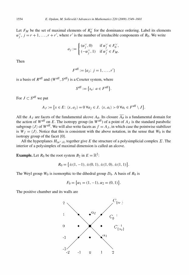
Example. Let R0 be the root system B2 in E = R2:
R0 = {±(1, −1), ±(0,1), ±(1,0), ±(1,1)}.
The Weyl group W0 is isomorphic to the dihedral group D4. A basis of R0 is
F0 = {α1 = (1, −1), α2 = (0,1)}.
The positive chamber and its walls are
E. Opdam, M. Solleveld / Advances in Mathematics 220 (2009) 1549–1601 1555
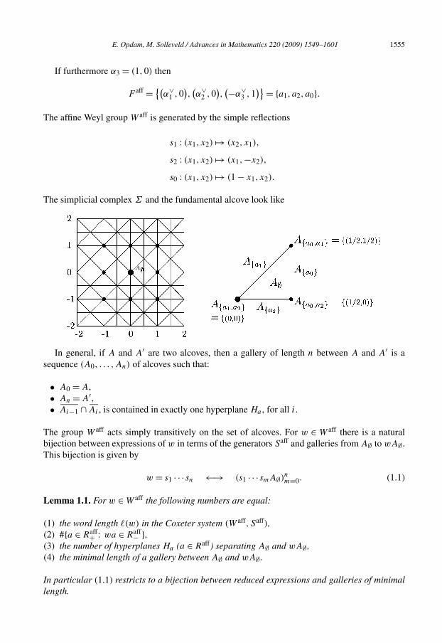
If furthermore α3 = (1,0) then
F aff = {(α∨1 ,0
),(α∨
2 ,0),(−α∨
3 ,1)} = {a1, a2, a0 }.
The affine Weyl group W aff is generated by the simple reflections
s1 : (x1, x2) �→ (x2, x1),
s2 : (x1, x2) �→ (x1, −x2),
s0 : (x1, x2) �→ (1 − x1, x2).
The simplicial complex Σ and the fundamental alcove look like
In general, if A and A′ are two alcoves, then a gallery of length n between A and A′ is asequence (A0, . . . ,An) of alcoves such that:
• A0 = A,• An = A′,• Ai−1 ∩ Ai , is contained in exactly one hyperplane Ha , for all i.
The group W aff acts simply transitively on the set of alcoves. For w ∈ W aff there is a naturalbijection between expressions of w in terms of the generators Saff and galleries from A∅ to wA∅.This bijection is given by
w = s1 · · · sn ←→ (s1 · · · smA∅)nm=0. (1.1)
Lemma 1.1. For w ∈ W aff the following numbers are equal:
(1) the word length �(w) in the Coxeter system (W aff, Saff),(2) #{a ∈ Raff+ : wa ∈ Raff− },(3) the number of hyperplanes Ha (a ∈ Raff) separating A∅ and wA∅,(4) the minimal length of a gallery between A∅ and wA∅.
In particular (1.1) restricts to a bijection between reduced expressions and galleries of minimallength.
1556 E. Opdam, M. Solleveld / Advances in Mathematics 220 (2009) 1549–1601
Proof. See [14, Section 1], [3, Section 2.1] or [13, Theorem 4.5]. �Varying on the Bruhat order, we define a partial order �A on the affine Weyl group W aff:
u �A w ⇐⇒ �(u) + �(u−1w
) = �(w).
This means that u �A w if and only if a reduced expression for u can be extended to a reducedexpression for w by writing extra terms on the right.
Let K be a subset of E, and α ∈ R0.
m(K,α) := inf{⌊〈x,α∨ 〉⌋: x ∈ K ∪ A∅
},
M(K,α) := sup{⌈〈x,α∨ 〉⌉: x ∈ K ∪ A∅
},
where �y� and �y� denote respectively the floor and the ceiling of a real number y. With thesenumbers we define
A(K,α) := {x ∈ E: m(K,α) � 〈x,α∨ 〉 � M(K,α)},
A(K) :=⋂
α∈R0
A(K,α).
We can interpret A(K) as a kind of Σ -approximation of the convex closure of K ∪ A∅ in E.
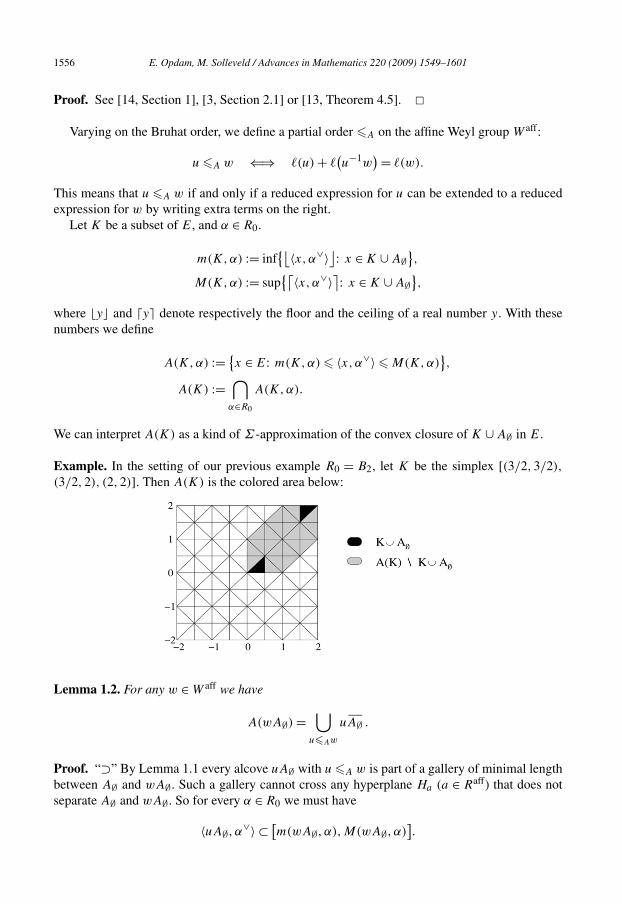
Example. In the setting of our previous example R0 = B2, let K be the simplex [(3/2,3/2),
(3/2,2), (2,2)]. Then A(K) is the colored area below:
Lemma 1.2. For any w ∈ W aff we have
A(wA∅) =⋃
u�Aw
uA∅ .
Proof. “⊃” By Lemma 1.1 every alcove uA∅ with u �A w is part of a gallery of minimal lengthbetween A∅ and wA∅. Such a gallery cannot cross any hyperplane Ha (a ∈ Raff) that does notseparate A∅ and wA∅. So for every α ∈ R0 we must have
〈uA∅, α∨ 〉 ⊂ [m(wA∅, α),M(wA∅, α)].

E. Opdam, M. Solleveld / Advances in Mathematics 220 (2009) 1549–1601 1557
“⊂” Since it is bounded by hyperplanes Ha with a ∈ Raff, A(wA∅) is a union of closuresof alcoves. If B ⊂ A(wA∅) is an alcove, then there are no hyperplanes Ha separating B fromA∅ ∪ wA∅. Hence B is part of at least one gallery of minimal length between A∅ and wA∅. SoB = uA∅ for some u �A w. �
We note the consequence
wA(σ) ⊂ A(wσ) ∀σ ⊂ C+∅ , w ∈ W0. (1.2)
1.2. Affine Hecke algebras
We recall a few important results on affine Hecke algebras, meanwhile fixing some notations.Reconsider the based root datum R = (X,R0, Y,R∨
0 ,F0). The extended affine Weyl group of Ris
W(R) = W = X � W0.
It acts naturally on X, and to avoid confusion we will often denote the element of W correspond-ing to x ∈ X by tx . For any x ∈ X and w ∈ W0 we have w(x) − x ∈ ZR0, so W(R) contains W aff
as a normal subgroup. We write
X+ := {x ∈ X: 〈x,α∨ 〉 � 0 ∀α ∈ F0},
X− := {x ∈ X: 〈x,α∨ 〉 � 0 ∀α ∈ F0} = −X+.
It is easily seen that the center of W is the lattice
Z(W) = X+ ∩ X−.
We also want to make W act on E. Since
X ⊗ R = E ⊕ (Z(W) ⊗ R
),
there is a canonical projection
pE : X ⊗ R → E.
This induces a group homomorphism
pE : W → E � W0,
and the latter group acts naturally on E. The resulting action of W on E consists of automor-phisms of Σ , because ⟨
pE(x),α∨⟩ = 〈x,α∨ 〉 ∈ Z ∀x ∈ X, α∨ ∈ R∨.
0
1558 E. Opdam, M. Solleveld / Advances in Mathematics 220 (2009) 1549–1601
Hence (2), (3) and (4) of Lemma 1.1 define a natural extension of the length function � fromW aff to W . The subgroup Ω := {ω ∈ W : �(ω) = 0} of W is complementary to W aff:
W = W aff � Ω.
We say that R is semisimple if R⊥0 = 0 ⊂ Y , or equivalently if X ⊗ R = E. If R is not semisimple
then we can make it so by enlarging R0 and R∨0 . Namely, pick a basis {αr+1, . . . , αrk(X)} of
X ∩ (R∨0 )⊥. Then
F0 = {α1, . . . , αrk(X)}is a basis of a root system
R0 ∼= R0 × (A1)rk(X)−r .
Furthermore, pick α∨j ∈ Y such that⟨
αi,α∨j
⟩ = 2δij , i = 1, . . . , rk(X), j > r.
This yields a semisimple based root datum
R := (X, R0, Y, R∨0 , F0
). (1.3)
Denoting the Weyl group of (A1)rk(X)−r by G, we observe that
W(R) = W(R) � G = X �(W0(R) × G
) = X � W0(R). (1.4)
With R we also associate some other root systems. There is the non-reduced root system
Rnr := R0 ∪ {2α: α∨ ∈ 2Y }.Obviously we put (2α)∨ = α∨/2. Let R1 be the reduced root system of long roots in Rnr :
R1 := {α ∈ Rnr : α∨ /∈ 2Y }.Let q be a positive labeling of R∨
nr , that is, a W0-invariant map R∨nr → (0, ∞). This uniquely
determines a parameter function q : W → (0, ∞) with the properties
q(sα∨ ) = qα∨ , α ∈ R0 ∩ R1,
q(s1+β∨ ) = qβ∨ , β ∈ R0 \ R1,
q(sβ∨ ) = qβ∨/2qβ∨ , β ∈ R0 \ R1,
q(ω) = 1, �(ω) = 0,
q(wv) = q(w)q(v), w,v ∈ W with �(wv) = �(w) + �(v). (1.5)
Conversely every function on W with the last two properties defines a labeling of R∨nr . We speak
of equal parameters if q(s) = q(s′) ∀s, s′ ∈ Saff.
E. Opdam, M. Solleveld / Advances in Mathematics 220 (2009) 1549–1601 1559
The affine Hecke algebra H = H(R, q) is the unique complex associative algebra with basis{Tw: w ∈ W } and relations
TwTv = Twv if �(wv) = �(w) + �(v),
TsTs = (q(s) − 1)Ts + q(s)Te if s ∈ Saff.
We can extend q to a parameter function q on W(R) by putting
q(sα∨j) = 1 ∀j > r. (1.6)
Then G acts on H(R, q) and its group algebra is naturally embedded in H(R, q), so the lattercan be regarded as a crossed product algebra:
H(R, q) ∼= G � H(R, q).
Now we describe the Bernstein presentation of H. For x ∈ X+ we put
θx := q(x)−1/2Tx.
The corresponding semigroup morphism X+ → H(R, q)× extends to a group homomorphism
X → H(R, q)× : x �→ θx.
Theorem 1.3 (Bernstein presentation).
(a) The sets {Twθx : w ∈ W0, x ∈ X} and {θxTw: w ∈ W0, x ∈ X} are bases of H.(b) The subalgebra A := span{θx : x ∈ X} is isomorphic to C[X].(c) The center of Z(H(R, q)) of H(R, q) is AW0 , where we define the action of W0 on A by
w · θx = θwx .
Proof. These results are due to Bernstein, see [19, §3]. �Let T be the complex algebraic torus HomZ(X,C×), so that A ∼= O(T ) and Z(H) = AW0 ∼=
O(T /W0). From Theorem 1.3 we see that H is of finite rank over its center, and hence Noethe-rian.
For a set of simple roots I ⊂ F0 we introduce the notations
RI = QI ∩ R0, R∨I = QR∨
I ∩ R∨0 ,
XI = X/(X ∩ (I ∨)⊥), XI = X/(X ∩ QI ),
YI = Y ∩ QI ∨, Y I = Y ∩ I ⊥,
TI = HomZ(XI ,C×), T I = HomZ
(XI ,C×),
RI = (XI ,RI ,YI ,R∨I , I
), RI = (X,RI ,Y,R∨
I , I). (1.7)
We can define parameter functions qI and qI on the root data RI and RI , as follows. Restrictq to a labeling of (RI )
∨ and use (1.5) to extend it to W(RI ) and W(RI ). Then H(RI , qI ) is
nr
1560 E. Opdam, M. Solleveld / Advances in Mathematics 220 (2009) 1549–1601
isomorphic to the subalgebra of H(R, q) generated by A and H(WI , q). With this identificationin mind we call H(RI , qI ) a parabolic subalgebra of H(R, q).
For any t ∈ T I there is a surjective algebra homomorphism
φt : H(
RI , qI) → H(RI , qI ),
φt (θxTw) = t (x)θxITw, (1.8)
where xI is the image of x ∈ X in XI . So given any representation σ of H(RI , qI ), we canconstruct the H-representation
π(I, σ, t) := IndH(R,q)
H(RI ,qI )(σ ◦ φt ).
Representations of this form are said to be parabolically induced.Since H is of finite rank over Z(H), every irreducible H-representation has finite dimension.
In particular an H-module is of finite length if and only if it has finite dimension. Let Mod(H)
be the category of all H-modules and Modfin(H) the subcategory of finite length H-modules.We denote the Grothendieck group of Modfin(H) by G(H) and we write
GC(H) := G(H) ⊗Z C.
Similarly we can define Mod(A), Modfin(A), G(A) and GC(A) for any algebra or group A.For bornological algebras A we will also consider the category Modbor(A) of bornological A-modules, see Appendix A.
The center of H(R, q) contains the group algebra of Z(W), so every irreducible H-representation admits a unique Z(W)-character χ . Such representations factor through the al-gebra
H(R, q)χ = H ⊗Z(W) Cχ .
The algebra H is endowed with a trace
τ
( ∑w∈W
hwTw
)= he
and an involution ( ∑w∈W
hwTw
)∗=∑w∈W
hwTw−1 .
Because q takes only positive values, ∗ is conjugate-linear and antimultiplicative, while τ ispositive.
Our affine Hecke algebra is canonically isomorphic to the crossed product of the Iwahori–Hecke algebra corresponding to W aff, and the group Ω :
H(R, q) ∼= H(W aff, q
)� Ω.
E. Opdam, M. Solleveld / Advances in Mathematics 220 (2009) 1549–1601 1561
Let f be a facet of the fundamental alcove A∅ and write
Ωf := {ω ∈ Ω: pEω(f ) = f}.
Whether or not ω changes the orientation of f is measured by the character εf : Ωf → {±1}.Furthermore Ωf acts on Wf , so we can define
H(R, f, q) := H(Wf , q) � Ωf .
We note that for any H(R, f, q)-module (π,V ) there is a well-defined H(R, f, q)-moduleV ⊗ εf , where
(π ⊗ εf )(hTω)(v) := εf (ω)π(hTω)(v).
By definition Z(W) ⊂ Ωf , so
C[Z(W)
] ⊂ Z(
H(R, f, q)).
Lemma 1.4. Let Cχ be a one-dimensional Z(W)-representation with character χ .
H(R, f, q)χ := H(R, f, q) ⊗Z(W) Cχ
is a finite dimensional semisimple algebra.
Proof. As vector spaces we may identify
H(R, f, q)χ = IndH(R,f,q)
C[Z(W)] Cχ = H(Wf , q) ⊗C C[Ωf /Z(W)
].
We can extend |χ | canonically to X ⊗ R, making it 1 on E. Using this extension we define aninvolution ∗χ on H(R, f, q) by
(hwTw)∗χ = hw |χ |(2w(0))Tw−1 .
The associated bilinear form is
〈h,h′ 〉χ = τ(h∗χ · h′).
By construction IndH(R,f,q)
C[Z(W)] Cχ is now a unitary representation. This makes H(R, f, q)χ into afinite dimensional Hilbert algebra, so in particular it is semisimple. �1.3. The Schwartz completion
We show how to complete an affine Hecke algebra to a C∗-algebra and to a Schwartz algebra.The involution and the trace on H(R, q) give rise to a Hermitian inner product
〈h,h′ 〉 = τ(h∗ · h′), h,h′ ∈ H(R, q),
1562 E. Opdam, M. Solleveld / Advances in Mathematics 220 (2009) 1549–1601
and a norm
‖h‖τ = √〈h,h〉 = √τ(h∗ · h).
With a basic calculation one can check that{Nw = q(w)−1/2Tw: w ∈ W
}(1.9)
is an orthonormal basis of H(R, q) for this inner product. All this gives H(R, q) the structureof a Hilbert algebra, in the sense of [10, A 54]. Let L2(R, q) be its Hilbert space completion, forwhich (1.9) is by definition a basis. Consider the multiplication map
λ(h) : H(R, q) → H(R, q),
λ(h)h′ = h · h′.
By [26, Lemma 2.3] this maps extends to a bounded operator on L2(R, q), whose norm wedenote by
‖h‖o = ∥∥λ(h)∥∥
B(L2(R,q)).
Thus, H(R, q) being a ∗-subalgebra of the C∗-algebra B(L2(R, q)) of bounded operators onL2(R, q), we can consider its closure C∗(R, q) with respect to the operator norm topology. Bydefinition this is a separable unital C∗-algebra, called the (reduced) C∗-algebra of H or of (R, q).
Let (π,V ) be an irreducible H-representation. We say that it belongs to the discrete series ifthe following equivalent conditions hold:
• (π,V ) is a subrepresentation of the left regular representation (λ,L2(R, q)),• all matrix coefficients of (π,V ) are in L2(R, q).
By definition a discrete series representation is unitary, and it extends continuously toC∗(R, q). Because this is a Hilbert algebra, a suitable version of [10, Proposition 18.4.2] showsthat π is an isolated point in its spectrum. Moreover, since C∗(R, q) is unital its spectrum iscompact [10, Proposition 3.18], so there can be only finitely many inequivalent discrete seriesrepresentations.
It is also possible to complete H(R, q) to a Schwartz algebra S = S(R, q). As a topologicalvector space S will consist of rapidly decreasing functions on W , with respect to some lengthfunction. For this purpose it is unsatisfactory that � is 0 on the subgroup Z(W), as this can be alarge part of W . To overcome this inconvenience, let L : X ⊗ R → [0, ∞) be a function such that
• L(X) ⊂ Z,• L(x + y) = L(x) ∀x ∈ X ⊗ R, y ∈ E,• L induces a norm on X ⊗ R/E ∼= Z(W) ⊗ R.
Now we define for w ∈ W
N (w) := �(w) + L(w(0)
),
E. Opdam, M. Solleveld / Advances in Mathematics 220 (2009) 1549–1601 1563
so that
N (uω) = N (ωu) = �(u) + L(ω(0)
), u ∈ W aff, ω ∈ Ω,
N (wv) � N (w) + N (v), w,v ∈ W.
Since Z(W) ⊕ ZR0 is of finite index in X, the set {w ∈ W : N (w) = 0} is finite. Moreover,because W is the semidirect product of a finite group and an abelian group, it is of polynomialgrowth and different choices of L lead to equivalent length functions N . For n ∈ N we define thenorm
pn
( ∑w∈W
hwNw
):= sup
w∈W
|hw |(N (w) + 1)n
.
The completion S = S(R, q) of H(R, q) with respect to the family of norms {pn}n∈N is a nuclearFréchet space. It consists of all possibly infinite sums h = ∑
w∈W hwNw such that pn(h) < ∞∀n ∈ N.
Lemma 1.5. (See [33, p. 135].) Let b = rk(X) + 1. The sum∑w∈W
(N (w) + 1
)−b
converges to a limit Cb . If h ∈ S and n ∈ N then∑w∈W |hw |(N (w) + 1
)n � Cbpn+b(h).
The norms pn behave reasonably with respect to multiplication:
Theorem 1.6. (See [26, Section 6.2].) There exist Cq > 0, d ∈ N, such that ∀h, h′ ∈ S(R, q),n ∈ N
‖h‖o � Cqpd(h),
pn(h · h′) � Cqpn+d(h)pn+d(h′).
In particular S(R, q) is a unital locally convex ∗-algebra, and it is contained in C∗(R, q).
A finite dimensional H-module is called tempered if the H-action extends continuously to S .There are various ways to define infinite dimensional tempered modules, depending on whichcategory of vector spaces one wishes to consider. In Appendix A we discuss tempered bornolog-ical modules.
From the work of Casselman [7, §4.4] one can deduce concrete criteria for representationsto be tempered or discrete series, see [26, Section 2.7]. It follows from these criteria that anH-module can only be tempered if all its Z(W)-weights are unitary.
The reader is referred to [9] for a study of the algebra S and its Fourier transform. Noticethat as a Fréchet space S(R, q) does not depend on q . The basis {Nw: w ∈ W } gives rise to acanonical isomorphism between S(R, q) and S(W).
1564 E. Opdam, M. Solleveld / Advances in Mathematics 220 (2009) 1549–1601
For ε ∈ R let qε be the parameter function qε(w) = q(w)ε . For every ε we have the affineHecke algebra H(R, qε) and its Schwartz completion S(R, qε). We note that H(R, q0) = C[W ]is the group algebra of W and that S(R, q0) = S(W) is the Schwartz algebra of rapidly decreas-ing functions on W .
The intuitive idea is that these algebras depend continuously on ε. We will use this in the formof the following rather technical result.
Theorem 1.7. For ε ∈ [−1,1] there exists a family of additive functors
σε : Modfin(
H(R, q)) → Modfin
(H(
R, qε))
,
σε(π,V ) = (πε,V )
with the properties
(1) the map
[−1,1] → EndV : ε �→ πε(Nw)
is analytic for any w ∈ W ,(2) σε is a bijection if ε = 0,(3) σε preserves unitarity,(4) σε preserves temperedness if ε � 0,(5) σε preserves the discrete series if ε > 0.
Proof. See [33, Theorem 5.16 and Lemma 5.17]. �2. Projective resolutions
In this section we will construct projective resolutions for modules of an affine Hecke alge-bra H. We do this in a functorial way, starting from an explicit projective H-bimodule resolutionof H. This allows us to show that the global dimension of H equals the rank of the lattice X.
It turns out that the same constructions also work over S . However this is by no means auto-matic. Namely, it is not enough to have a projective H-bimodule resolution, to show that it can beinduced to S we also need a contraction which is bounded in a suitable sense. The essential partof the proof takes place within the polysimplicial complex Σ associated to the root system R0.Taking advantage of the abundant symmetry of root systems we construct a bounded contrac-tion of the corresponding differential complex. With this contraction we establish a projectivebimodule resolution of S . As a consequence we can show that the cohomological dimension ofbornological S -modules also equals the rank of X.
Actually more is true, as Ralf Meyer kindly pointed out to us. The inclusion of complete, uni-tal, bornological algebras H → S is isocohomological (in the sense discussed in Appendix A).
2.1. The bounded contraction of the polysimplicial complex
From the polysimplicial complex Σ (cf. page 1554) we construct a differential complex(C∗(Σ), ∂∗). The vector space in degree n is
Cn(Σ) := C{σ ∈ Σ : dimσ = n}. (2.1)
E. Opdam, M. Solleveld / Advances in Mathematics 220 (2009) 1549–1601 1565
For every σ there is a unique facet f of the fundamental alcove A∅ such that σ is W aff-conjugateto the closure f of f in E. We fix an orientation on all the facets of A∅ and we decree that themap w : f → wf preserves orientation. This determines a unique orientation on every simplexof Σ . With these conventions we can identify
Cn(Σ) =⊕
f : dimf =n
C[W aff/Wf
]. (2.2)
Clearly Σ is the direct product of a number (say r ′) simplicial complexes corresponding to theirreducible components of R0. Let
σ = σ (1) × · · · × σ (r ′)
be a polysimplex of Σ . Denote the vertices of σ (j) by x(j)i , so that we can write
σ (j) = [x(j)
0 , x(j)
1 , . . . , x(j)dj
].
The order of the vertices defines an orientation on σ (j). For a permutation λ ∈ Sdjwith sign ε(λ)
we identify [x
(j)
λ(0), x(j)
λ(1), . . . , x(j)
λ(dj )
] = ε(λ)[x
(j)
0 , x(j)
1 , . . . , x(j)dj
].
The boundary of σ (j) is defined as
∂σ (j) = ∂[x
(j)
0 , x(j)
1 , . . . , x(j)dj
] :=dj∑i=0
(−1)i[x
(j)
0 , . . . , x(j)
i−1, x(j)
i+1, . . . , x(j)dj
],
∂[x
(j)
0
] := 0.
Furthermore we define
∂nσ =r ′∑
j =1
(−1)d1 +···+dj −1σ (1) × · · · × σ (j −1) × ∂σ (j) × σ (j +1) × · · · × σ (r ′)
if dimσ = n > 0. It is easily verified that this operation satisfies the usual property ∂ ◦ ∂ = 0. Weaugment this differential complex by
C−1(Σ) = C
and ∂0 [x] = 1 if x is a vertex of Σ . The augmented complex (C∗(Σ), ∂∗) computes the reducedsingular homology of the space E underlying Σ . This space is contractible, so by the Poincarélemma
Hn
(C∗(Σ), ∂∗
) = 0 ∀n ∈ Z. (2.3)
1566 E. Opdam, M. Solleveld / Advances in Mathematics 220 (2009) 1549–1601
The support of a chain c = ∑σ ∈Σ cσ σ ∈ C∗(Σ) is
supp c =⋃
σ : cσ =0
σ.
A contraction γ of (C∗(Σ), ∂∗) is a collection of linear maps
γn : Cn(Σ) → Cn+1(Σ), n � −1,
such that
γn−1∂n + ∂n+1γn = idCn(Σ) ∀n ∈ Z.
The periodic nature of Σ allows us to construct a contraction with good bounds on the coeffi-cients:
Proposition 2.1. There exists a contraction γ with the properties
(1) γ ∂ + ∂γ = id,(2) γ is W0-equivariant,(3) suppγ (σ ) ⊂ A(σ) for every σ ∈ Σ ,(4) γ (σ ) = ∑τ ∈Σ γστ τ with |γστ | < Mγ for some constant Mγ depending only on γ .
Proof. Our construction will be rather similar to that of V. Lafforgue in [32, §4]. First we imposesome extra conditions. (2) and (3) force
(5) if σ ⊂ C+I then suppγ (σ ) ⊂ C+
I .
In view of (1.2) and since ∂ is W0-equivariant, it suffices to construct γ on C+∅ . We will use that
the translations tx with x ∈ ZR0 are orientation preserving automorphisms of Σ . For αi ∈ F0let βi be the minimal element of C++
F0 \{αi } ∩ ZR0. Note that βi is an integral multiple of a vertexof A∅. We could also pick a fundamental weight instead of βi , but in that case we would havekeep track of the orientations. Consider the halfopen parallelogram
P∅ ={
r∑i=1
yiβi : yi ∈ [0,1)
}.
Let τ be any polysimplex whose interior is contained in P∅. Our contraction will also satisfy
(6) γ (t(m+1)βi(τ )) = γ (tmβi
(τ )) + tmβiγ (tβi
(τ ) − τ)
for m � 0. Suppose that β = ∑ki=1 niβi with ni ∈ N. Then we decree
(7) γ (tβ(τ )) = γ (tnkβk(τ )) + tnkβk
γ (tβ−nkβk(τ ) − τ).
Here we use the ordering on the set F0 of simple roots. The idea underlying (6) and (7) is thatwe want to make γ equivariant with respect to certain translations.
E. Opdam, M. Solleveld / Advances in Mathematics 220 (2009) 1549–1601 1567
Now we really start constructing γ . In degree −1 we put
γ−1(1) = [0].Suppose that γm has already been defined for m < n, satisfying conditions (1)–(7). Let σ be anyn-dimensional polysimplex whose interior is contained in
P1 := P∅ ∪ tβ1P∅ ∪ · · · ∪ tβr P∅.
By (1) we have
∂(σ − γ ∂(σ )
) = (id − ∂γ )(∂σ ) = γ ∂(∂σ ) = 0.
Together with (2.3) this implies that the equation
∂γ (σ ) = σ − γ ∂(σ )
has a solution γ (σ ) ∈ Cn+1(Σ). By (3) and (5) we have
supp(σ − γ ∂(σ )
) ⊂ A(σ) ∩ C+I if σ ⊂ C+
I .
Since A(σ) ∩ C+I is convex, we can pick γ (σ ) with support in this set. We do this for any n-
dimensional σ ∈ Σ whose interior is contained in P1. Now (6) and (7) determine γn uniquelyon C+
∅ .We will show that the other required properties follow from this construction. Write β ′ =∑k−1i=1 niβi and β ′ ′ = ∑k−1
i=1 n′iβi for some n′
i ∈ N. By (7) we have
γ tnkβk
(tβ ′ (τ ) − tβ ′ ′ (τ )
) = tnkβkγ(tβ ′ (τ ) − tβ ′ ′ (τ )
). (2.4)
We claim that the following stronger version of (7) holds
(7′) γ tnkβk(tβ−nkβk
(σ ) − σ) = tnkβkγ (tβ−nkβk
(σ ) − σ) ∀σ ⊂ C+∅ .
Indeed, write σ = txτ with τ as in (7) and x = ∑rj =1 mjβj . Then by a repeated application of
(2.4) the left-hand side of (7′) becomes
γ tnkβk
(tβ ′ (txτ ) − txτ
) = t(nk +mk)βk +mk+1βk+1 +···+mrβr γ (tβ ′ − id)tm1β1 +···+mk−1βk−1(τ )
= tnkβkγ tx(tβ ′ (τ ) − τ
)= tnkβk
γ(tβ ′ (σ ) − σ
).
It follows easily from (6) that
γ tmβi
(tm′βi
(τ ) − tm′ ′βi(τ )) = tmβi
γ(tm′βi
(τ ) − tm′ ′βi(τ )) ∀m,m′,m′ ′ ∈ N. (2.5)
There also is a stronger version of (6):
(6′) γ tmβ (tβ (σ ) − σ) = tmβ γ (tβ (σ ) − σ) ∀σ ⊂ C+ .
i i i i ∅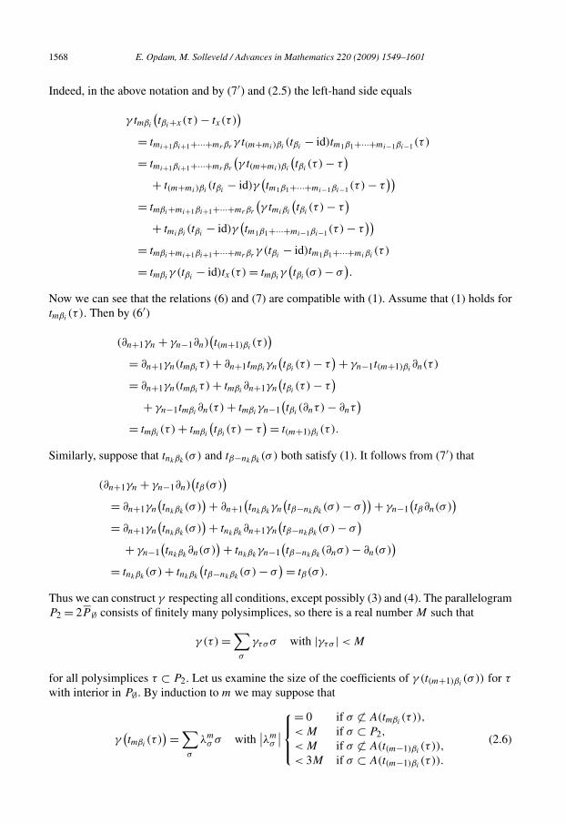
1568 E. Opdam, M. Solleveld / Advances in Mathematics 220 (2009) 1549–1601
Indeed, in the above notation and by (7′) and (2.5) the left-hand side equals
γ tmβi
(tβi +x(τ ) − tx(τ )
)= tmi+1βi+1 +···+mrβr γ t(m+mi)βi
(tβi− id)tm1β1 +···+mi−1βi−1(τ )
= tmi+1βi+1 +···+mrβr
(γ t(m+mi)βi
(tβi
(τ ) − τ)
+ t(m+mi)βi(tβi
− id)γ(tm1β1 +···+mi−1βi−1(τ ) − τ
))= tmβi +mi+1βi+1 +···+mrβr
(γ tmiβi
(tβi
(τ ) − τ)
+ tmiβi(tβi
− id)γ(tm1β1 +···+mi−1βi−1(τ ) − τ
))= tmβi +mi+1βi+1 +···+mrβr γ (tβi
− id)tm1β1 +···+miβi(τ )
= tmβiγ (tβi
− id)tx(τ ) = tmβiγ(tβi
(σ ) − σ).
Now we can see that the relations (6) and (7) are compatible with (1). Assume that (1) holds fortmβi
(τ ). Then by (6′)
(∂n+1γn + γn−1∂n)(t(m+1)βi
(τ ))
= ∂n+1γn(tmβiτ ) + ∂n+1tmβi
γn
(tβi
(τ ) − τ)+ γn−1t(m+1)βi
∂n(τ )
= ∂n+1γn(tmβiτ ) + tmβi
∂n+1γn
(tβi
(τ ) − τ)
+ γn−1tmβi∂n(τ ) + tmβi
γn−1(tβi
(∂nτ ) − ∂nτ)
= tmβi(τ ) + tmβi
(tβi
(τ ) − τ) = t(m+1)βi
(τ ).
Similarly, suppose that tnkβk(σ ) and tβ−nkβk
(σ ) both satisfy (1). It follows from (7′) that
(∂n+1γn + γn−1∂n)(tβ(σ )
)= ∂n+1γn
(tnkβk
(σ ))+ ∂n+1
(tnkβk
γn
(tβ−nkβk
(σ ) − σ))+ γn−1
(tβ∂n(σ )
)= ∂n+1γn
(tnkβk
(σ ))+ tnkβk
∂n+1γn
(tβ−nkβk
(σ ) − σ)
+ γn−1(tnkβk
∂n(σ ))+ tnkβk
γn−1(tβ−nkβk
(∂nσ ) − ∂n(σ ))
= tnkβk(σ ) + tnkβk
(tβ−nkβk
(σ ) − σ) = tβ(σ ).
Thus we can construct γ respecting all conditions, except possibly (3) and (4). The parallelogramP2 = 2P ∅ consists of finitely many polysimplices, so there is a real number M such that
γ (τ) =∑σ
γτσ σ with |γτσ | < M
for all polysimplices τ ⊂ P2. Let us examine the size of the coefficients of γ (t(m+1)βi(σ )) for τ
with interior in P∅. By induction to m we may suppose that
γ(tmβi
(τ )) =
∑σ
λmσ σ with
∣∣λmσ
∣∣⎧⎪⎨⎪⎩
= 0 if σ ⊂ A(tmβi(τ )),
< M if σ ⊂ P2,
< M if σ ⊂ A(t(m−1)βi(τ )),
(2.6)
< 3M if σ ⊂ A(t(m−1)βi(τ )).
E. Opdam, M. Solleveld / Advances in Mathematics 220 (2009) 1549–1601 1569
By construction we have
tmβiγ(tβi
(τ ) − τ) =
∑σ
λ′σ σ with
∣∣λ′σ
∣∣⎧⎪⎨⎪⎩
= 0 if σ ⊂ A(t(m+1)βi(τ )),
= 0 if σ ⊂ tmβiC+
∅ ,
< M if σ ⊂ A(tmβi(τ )),
< 2M if σ ⊂ A(t(m+1)βi(τ )).
With (6) this implies that (2.6) also holds with m + 1 instead of m.Let β be as above. By induction to k we may assume that
tnkβkγ(tβ−nkβk
(τ ) − τ) =
∑σ
μkσ σ with
∣∣μkσ
∣∣⎧⎪⎪⎪⎨⎪⎪⎪⎩
= 0 if σ ⊂ A(tβ(σ )),
= 0 if σ ⊂ tnkβkC+
∅ ,
< M if σ ⊂ tβ ′ (σ ),
< 2M if σ ⊂ A(tnkβk(σ )),
< 3M if σ ⊂ A(tβ(σ )),
(2.7)
where β ′ = β − βi with i minimal for ni > 0. In view of (7) the above implies that
γ(tβ(τ )
) =∑σ
μ′σ σ with
∣∣μ′σ
∣∣⎧⎪⎨⎪⎩
= 0 if σ ⊂ A(tβ(σ )),
< M if σ ⊂ P2,
< M if σ ⊂ A(tβ ′ (σ )),
< 3M if σ ⊂ A(tβ(σ )).
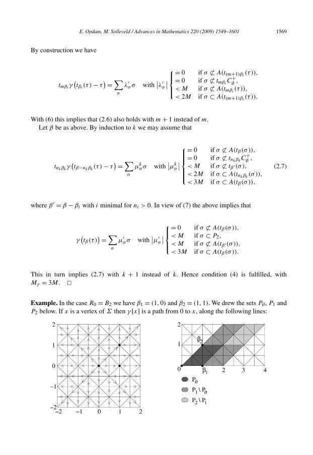
This in turn implies (2.7) with k + 1 instead of k. Hence condition (4) is fulfilled, withMγ = 3M . �Example. In the case R0 = B2 we have β1 = (1,0) and β2 = (1,1). We drew the sets P∅, P1 andP2 below. If x is a vertex of Σ then γ [x] is a path from 0 to x, along the following lines:
1570 E. Opdam, M. Solleveld / Advances in Mathematics 220 (2009) 1549–1601
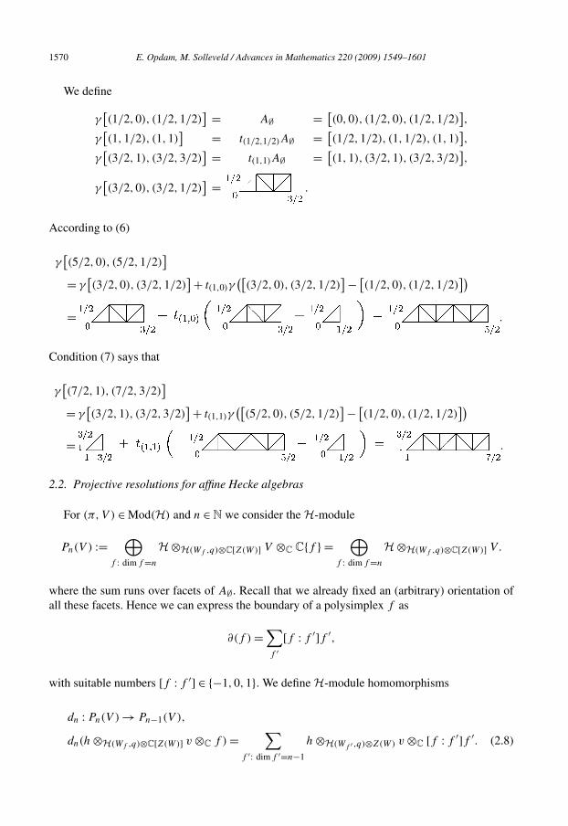
We define
γ[(1/2,0), (1/2,1/2)
] = A∅ = [(0,0), (1/2,0), (1/2,1/2)
],
γ[(1,1/2), (1,1)
] = t(1/2,1/2)A∅ = [(1/2,1/2), (1,1/2), (1,1)
],
γ[(3/2,1), (3/2,3/2)
] = t(1,1)A∅ = [(1,1), (3/2,1), (3/2,3/2)
],
γ[(3/2,0), (3/2,1/2)
] = .
According to (6)
γ[(5/2,0), (5/2,1/2)
]= γ
[(3/2,0), (3/2,1/2)
]+ t(1,0)γ([
(3/2,0), (3/2,1/2)]− [(1/2,0), (1/2,1/2)
])= .
Condition (7) says that
γ[(7/2,1), (7/2,3/2)
]= γ
[(3/2,1), (3/2,3/2)
]+ t(1,1)γ([
(5/2,0), (5/2,1/2)]− [(1/2,0), (1/2,1/2)
])= .
2.2. Projective resolutions for affine Hecke algebras
For (π,V ) ∈ Mod(H) and n ∈ N we consider the H-module
Pn(V ) :=⊕
f : dimf =n
H ⊗H(Wf ,q)⊗C[Z(W)] V ⊗C C{f } =⊕
f : dimf =n
H ⊗H(Wf ,q)⊗C[Z(W)] V.
where the sum runs over facets of A∅. Recall that we already fixed an (arbitrary) orientation ofall these facets. Hence we can express the boundary of a polysimplex f as
∂(f ) =∑f ′
[f : f ′ ]f ′,
with suitable numbers [f : f ′ ] ∈ {−1,0,1}. We define H-module homomorphisms
dn : Pn(V ) → Pn−1(V ),
dn(h ⊗H(Wf ,q)⊗C[Z(W)] v ⊗C f ) =∑
f ′ : dimf ′ =n−1
h ⊗H(Wf ′ ,q)⊗Z(W) v ⊗C [f : f ′ ]f ′. (2.8)
E. Opdam, M. Solleveld / Advances in Mathematics 220 (2009) 1549–1601 1571
Furthermore we define
d0 : P0(V ) → V,
d0(h ⊗H(Wx,q)⊗C[Z(W)] v ⊗C x) = π(h)v, (2.9)
if x is a vertex of A∅. Now (P∗(V ), d∗) is an augmented differential complex because ∂ ◦ ∂ = 0.The group Ω acts naturally on this complex by
ω(h ⊗H(Wf ,q)⊗C[Z(W)] v ⊗ f ) = hT −1ω ⊗H(Wω(f ),q)⊗C[Z(W)] π(Tω)v ⊗ ω(f ),
where we consider ω(f ) with orientation. This action commutes with the H-action and with thedifferentials dn, so (P∗(V )Ω,d∗) is again an augmented differential complex. Note that Pn(V )
and Pn(V )Ω are finitely generated H-modules if V has finite dimension.
Theorem 2.2. Consider H as an H-bimodule.
0 ←− H d0←− P0(H)Ωd1←− P1(H)Ω ←− · · · dr←− Pr(H)Ω ←− 0 (2.10)
is a resolution of H by H ⊗ Hop-modules. Every Pn(H)Ω is projective as a left and as a rightH-module. Moreover if R is semisimple then Pn(H)Ω is projective as a H ⊗ Hop-module.
Proof. This result stems from joint work of Mark Reeder and the first author, see [27, Proposi-tion 8.1]. The proof is based on constructions of Kato [15].
First we consider the case Ω = Z(W) = {e}, W = W aff. There is a linear bijection
φ : C[W ] ⊗C H → H ⊗C H,
φ(w ⊗ h′) = Tw ⊗ T −1w h′. (2.11)
For si ∈ Saff we write qi = q(si) and
Li := span{hTsi ⊗ T −1
sih′ − h ⊗ h′: h,h′ ∈ H
} ⊂ H ⊗C H,
C[W ]i :={ ∑
w∈W
xww: xwsi = −xw ∀w ∈ W
}⊂ C[W ]. (2.12)
This Li is interesting because
H ⊗ H(Wf ,q) H = (H ⊗C H)/ ∑
si ∈Wf
Li.
Let w ∈ W be such that �(wsi) > �(w). For any h′ ∈ H we have
φ((wsi − w) ⊗ h′) = Twsi ⊗ T −1
wsih′ − Tw ⊗ T −1
w h′ = TwTsi ⊗ T −1si
T −1w h′ − Tw ⊗ T −1
w h′ ∈ Li,
so φ(C[W ]i ⊗ H) ⊂ Li . On the other hand, Li is spanned by elements as in (2.12) with h = Tw
or h = Tws :
i
1572 E. Opdam, M. Solleveld / Advances in Mathematics 220 (2009) 1549–1601
φ−1(Twsi Tsi ⊗ T −1si
h′ − Twsi ⊗ h′)= φ−1(qiTw + (qi − 1)Twsi ⊗ T −1
sih′)− wsi ⊗ Twsi h
′
= qiw ⊗ TwT −1si
h′ + (qi − 1)wsi ⊗ Twsi T−1si
h′ − wsi ⊗ Twsi h′
= qi(w − wsi) ⊗ TwT −1si
h′ + wsi ⊗ (qiTwT −1
si+ (qi − 1)Twsi T
−1si
− Twsi
)h′
= (w − wsi) ⊗ TwqiT−1si
h′ + wsi ⊗ (Tw(Tsi + 1 − qi) + (qi − 1)Tw − TwTsi
)h′
= (w − wsi) ⊗ Tw(Tsi + 1 − qi)h′ ∈ C[W ]i ⊗ H.
We conclude that φ−1(Li) = C[W ]i ⊗ H. Now we bring the linear bijections
C[W ]/ ∑si ∈Wf
C[W ]i → C[W/Wf ] : w �→ wWf (2.13)
into play. Under these identifications our differential complex becomes
0 ← H ← · · · ←⊕
f : dimf =n
C[W/Wf ] ⊗ H ⊗ C{f } ← · · · ← C[W ] ⊗ H ⊗ C{A∅ } ← 0.
But this is just the complex (C∗(Σ), ∂∗) tensored with H, so by (2.3) its homology vanishes.This shows that indeed we have a resolution in the special case Ω = {e}.
Now the general case. Since the action of Ω on A∅ factors through the finite group Ω/Z(W)
we can construct a Reynolds operator
RΩ := [Ω : Z(W)]−1 ∑
ω∈Ω/Z(W)
ω ∈ EndH ⊗ Hop(Pn(H)
).
Since this is an idempotent,
Pn(H)Ω = RΩ · Pn(H) (2.14)
is a direct summand of Pn(H). We generalize (2.11) to a bijection
φ : C[W/Z(W)
]⊗C H → H ⊗C[Z(W)] H,
φ(w ⊗ h′) = Tw ⊗ T −1w h′. (2.15)
Just as above this leads to bijections⊕f : dimf =n
C[W/(Wf × Z(W)
)]⊗ H ⊗ C{f } → Pn(H). (2.16)
The group Ω/Z(W) acts on the left-hand side by
ω · (w ⊗ h′ ⊗ f ) = wω−1 ⊗ h′ ⊗ ω(f ).
Since both sides of (2.16) are free Ω/Z(W)-modules, we also get a linear bijection
E. Opdam, M. Solleveld / Advances in Mathematics 220 (2009) 1549–1601 1573
⊕f : dimf =n
C[W aff/Wf
]⊗ H ⊗ C{f } → Pn(H)Ω,
w ⊗ h′ ⊗ f �→ RΩ
(Tw ⊗H(Wf ,q)⊗C[Z(W)] T −1
w h′ ⊗ f). (2.17)
Now the same argument as in the special case shows that the modules Pn(H)Ω form a resolutionof H.
For any facet f , H is a free H(Wf , q) ⊗ C[Z(W)]-module, both from the left and from theright. Therefore every Pn(H) is a projective H-module, from the left and from the right.
For R semisimple Pn(H) is a direct sum of H ⊗ Hop-modules of the form H ⊗H(Wf ,q) H. Forevery irreducible representation Vi of H(Wf , q) we pick an idempotent ei ∈ H(Wf , q) whichacts as a rank one projection on Vi and as 0 on all other irreducible representations. Consider theelement ef = ∑i ei ⊗ ei ∈ H ⊗ Hop. From
H ⊗H(Wf ,q) H ∼= (H ⊗C Hop)ef (2.18)
we see that Pn(H) is a projective H-bimodule. By (2.14) Pn(H)Ω is projective in the same sensesas Pn(H). �Corollary 2.3.
(a) Let V be any H-module.
0 ←− Vd0←− P0(V )Ω
d1←− P1(V )Ω ←− · · · dr←− Pr(V )Ω ←− 0
is a resolution of V . It is bornological if V is.(b) If V admits a Z(W)-character χ then every Pn(V )Ω is a projective H(R, q)χ -module.(c) The cohomological dimensions of Mod(H(R, q)χ ) and Modbor(H(R, q)χ ) equal r =
rk(R0).
Proof. (a) Apply ⊗HV to (2.10). The resulting differential complex is exact because H andPn(H)Ω are projective right H-modules. For V ∈ Modbor(H) this clearly gives a bornologicaldifferential complex. It is split exact because every contraction of P∗(H)Ω yields a boundedsplitting of P∗(V )Ω .
(b) From
H ⊗ H(Wf ,q)⊗C[Z(W)] V ∼= H(R, q)χ ⊗H(Wf ,q) V ∼= IndH(R,q)χ
H(Wf ,q)V (2.19)
we see that this a projective H(R, q)χ -module. Hence Pn(V ) also has this property. It followsfrom (2.14) that
Pn(V )Ω = RΩ · Pn(V ) (2.20)
is a direct summand of Pn(V ).(c) By (a) and (b) these cohomological dimensions are at most r . On the other hand, we can
easily find modules which do not have projective resolutions of length smaller than r . Note that
Aχ := A ⊗Z(W) Cχ∼= O(Tχ ),
1574 E. Opdam, M. Solleveld / Advances in Mathematics 220 (2009) 1549–1601
where Tχ is the r-dimensional subtorus of T consisting of elements t such that t |Z(W) = χ . Pickt ∈ Tχ and consider the parabolically induced module
It = IndHA (Ct ) = Ind
H(R,q)χ
Aχ(Ct ). (2.21)
With Theorem 1.3 we find
ExtrH(R,q)χ(It , It ) ∼= ExtrAχ
(Ct , It ) ∼= ExtrO(Tχ )
(Ct ,
⊕w∈W0
Cwt
)∼=
⊕w∈W0: wt =t
Cwt . (2.22)
Since this space is not 0, any resolution of It by projective H(R, q)χ -modules has length atleast r .
This calculation goes through in the bornological setting, if we endow all spaces with the finebornology. �
For purposes of homological algebra it would be useful if we could also construct projectiveresolutions for H-modules that do not admit a Z(W)-character. Unfortunately the authors do notknow how to achieve this in general. But we offer an alternative that comes quite close. Let
H := H(R, q) = G � H(R, q)
be a semisimple affine Hecke algebra as in (1.3). Obviously H is a free (left or right) H-modulewith basis {Tg: g ∈ G}. Moreover for (π,V ) ∈ Mod(H) the H-module
IndHHV = H ⊗H V (2.23)
is isomorphic as an H-module to⊕
g∈G Vg , where the H-module structure on Vg = (πg,V ) isgiven by
πg(h)v = π(T −1
g hTg
)v. (2.24)
Clearly Vg = V as an H(RF0 , q)-module. If V admits a Z(W)-character χ , then Vg differs onlyfrom V in the sense that its Z(W)-character is gχ .
Applying the construction of Corollary 2.3(a) to H ⊗H V as an H-module we get a resolutionby modules that are projective in Mod(H) and in Mod(H). In several cases this might be used tofind a resolution of (π,V ) by projective H-modules.
Proposition 2.4. The cohomological dimensions of Mod(H) and Modbor(H) are both equal tothe rank of X.
Proof. The cohomological dimension of Mod(H) is the least number d ∈ {0,1,2, . . . , ∞} suchthat
Extn (U,V ) = 0 ∀U,V ∈ Mod(H), ∀n > d.
H
E. Opdam, M. Solleveld / Advances in Mathematics 220 (2009) 1549–1601 1575
Let t ∈ T and consider the module It = IndHA (Ct ). In view of Theorem 1.3
Extrk(X)
H (It , It ) ∼= Extrk(X)
A (Ct , It ) ∼= Extrk(X)
O(T )
(Ct ,
⊕w∈W0
Cwt
)∼=
⊕w∈W0: wt =t
Cwt .
Therefore d � rk(X). This argument also works in Modbor(H), provided that we endow allspaces with the fine bornology.
On the other hand, let U,V ∈ Mod(H) be arbitrary and consider the H-modules IndHH(U)
and IndHH(V ).
ExtnH(U,V ) ⊂⊕g∈G
ExtnH(U,Vg) ∼= ExtnH(U, IndH
H(V ))
∼= ExtnH(IndH
H(U), IndHH(V )
). (2.25)
Assume n > rk(X). According to Corollary 2.3(c) the cohomological dimension of Mod(H) isrk(X), so the right-hand side of (2.25) is 0. Hence ExtnH(U,V ) = 0 and we conclude that d �rk(X). The same reasoning shows that the cohomological dimension of Modbor(H) is rk(X). �
Recall that a resolution (P∗, d∗) of a module V is of finite type if all the modules Pn arefinitely generated, and moreover Pn = 0 for all n larger than some number.
Corollary 2.5. Let V be a finitely generated H-module. Then V admits a finite type projectiveresolution.
Proof. Because H is Noetherian, every submodule of a finitely generated H-module is itselffinitely generated.
By assumption there exist a surjective H-module map d0 : Hm0 → V , for some m0 ∈ N.Then kerd0 is again finitely generated, so we can find a surjection d1: Hm1 → kerd0. Continuingthis process we construct a resolution (Pn = Hmn, dn) of V , consisting of free H-modules offinite rank. Because the global dimension of H is rk(X), the module kerdn must be projective∀n � rk(X) − 1 [6, Proposition VI.2.1]. Hence
0 ←− Vd0←− P0
d1←− · · · dn−1←− Pn−1 ←− kerdn−1 ←− 0
is a finite type projective resolution of V . �2.3. Projective resolutions for Schwartz algebras
We will show that all the resolutions from the previous section can be induced from H to S .Most importantly, we will construct a projective bimodule resolution of S . This requires that wecomplete the H-modules to Fréchet S -modules. A convenient technique to achieve this in greatgenerality is with completed bornological tensor products, and this is the viewpoint we chose totake in this section. The necessary background material is contained in Appendix A. However,for finite dimensional tempered modules it is not necessary to use bornologies. See the remarkafter Corollary 2.7.
1576 E. Opdam, M. Solleveld / Advances in Mathematics 220 (2009) 1549–1601
Endow S with the precompact bornology and let V be a bornological S -module. Accordingto [22, Theorem 42] we have
S(Z(W)
) ⊗C[Z(W)] V = S(Z(W)
) ⊗ S(Z(W)) V . (2.26)
If V has finite dimension, then (2.26) also holds with algebraic tensor products. The reader isinvited to check this, by reduction to the case where V admits a unique Z(W)-character.
Because H is a free H(Wf , q) ⊗ C[Z(W)]-module, both algebraically and with the finebornology, we have
H ⊗H(Wf ,q)⊗C[Z(W)] V = H ⊗ H(Wf ,q)⊗C[Z(W)] V. (2.27)
So if we induce Pn(V ) from H to S in the bornological fashion we get the module
P tn(V ) := S ⊗H Pn(V ) = S ⊗ H
⊕f : dimf =n
H ⊗H(Wf ,q)⊗C[Z(W)] V ⊗C C{f }
=⊕
f : dimf =n
S ⊗H(Wf ,q)⊗ S(Z(W)) V ⊗C C{f }. (2.28)
The maps dn : Pn(V ) → Pn−1(V ) extend naturally to
dtn : P t
n(V ) → P tn−1(V ).
The action of Ω on Pn(V ) also extends to P tn(V ), so we can construct P t
n(V )Ω . By (2.14)
P tn(V )Ω = RΩ · P t
n(V ) (2.29)
is a direct summand of P tn(V ). Clearly P t
n(V ) and P tn(V )Ω are finitely generated S -modules if
V has finite dimension.We consider the important case V = S . The topology and the bornology on S give rise to a
topology and a bornology on P tn(S). For n,m,k ∈ N, f ⊂ A∅ we have the continuous seminorms
pm,k,f : S ⊗H(Wf ,q)⊗ S(Z(W)) S ⊗C C{f } → [0, ∞),
pm,k,f (y) = inf
{∑i
pm(hi)pk
(h′
i
):∑
i
hi ⊗ h′i ⊗ f = y
},
which define a Fréchet topology on this space. The topology on P tn(S) is defined by the norms
pm,k := ∑f pm,k,f . We endow these modules with the precompact bornology. We note that dt
n
is continuous and bounded and that Pn(S) is dense in P tn(S).
In view of (2.18) we have
P tn(S)Ω =
⊕f : dimf =n
S(RF0, q) ⊗H(Wf ,q) S(R, q) ∼=⊕
f : dimf =n
(S(RF0, q) ⊗C S(R, q)op)ef .
E. Opdam, M. Solleveld / Advances in Mathematics 220 (2009) 1549–1601 1577
Using Lemma 1.5 and Theorem 1.6 both for S(RF0, q) and for S(R, q) we see that there is anumber Cm,k,f > 0 such that
∑w∈W aff,w′ ∈W
|hw,w′ |(N (w) + 1)m(N (w′) + 1
)k� C2
b supw∈W aff,w′ ∈W
|hw,w′ |(N (w) + 1)m+b(N (w′) + 1
)k+b
� C2bpm+b,k+b
( ∑w∈W aff,w′ ∈W
hw,w′(Nw ⊗ N ′
w
)ef ⊗ f
)
� Cm,k,f pm+2b,k+2b,f
( ∑w∈W aff
∑w′ ∈W
hw,w′ Nw ⊗ Nw′)
. (2.30)
Theorem 2.6. Consider S as an S -bimodule.
0 ←− Sdt
0←− P t0(S)Ω
dt1←− P t
1(S)Ω ←− · · · dtr←− P t
r (S)Ω ←− 0 (2.31)
is an S ⊗ S op-module resolution of S , with a continuous bounded contraction. Every P tn(S) is
a bornologically projective S -module, both from the left and from the right. If moreover R issemisimple, then P t
n(S) is also projective as an S ⊗ S op-module.
Proof. To show that the differential complex (P t∗ (S)Ω, dt∗) is contractible we use Proposition 2.1and Theorem 2.2. The composition of (2.17) with (2.2) is the bijection
φ : C∗(Σ) ⊗C S → P∗(S)Ω,
φ(σ ⊗ h′) = RΩ
(Tw ⊗H(Wf ,q)⊗C[Z(W)] T −1
w h′ ⊗ f),
where σ = wf with w ∈ W aff. Let γ be as in Proposition 2.1. We claim that
γ := φ(γ ⊗ idS )φ−1
extends continuously to the required contraction. Suppose that w′ ∈ W , w ∈ W aff ∩ w′Ω andσ = w′f = wf . Then we have explicitly
φ(RΩ(Nw′ ⊗H(Wf ,q)⊗C[Z(W)] h′ ⊗ f )
) = φ(γ (σ ) ⊗ Nwh′) = φ
(∑τ
γστ τ ⊗ Nwh′)
. (2.32)
By Lemma 1.2 and condition (3) of Proposition 2.1 the coefficient γστ can only be nonzeroif there exist u �A w and a facet f ′ of A∅ such that τ = uf ′. This is crucial for the followingestimates. For every relevant τ we pick such a u ∈ W aff and we write (a little sloppily) γwu = γστ .Then (2.32) equals
1578 E. Opdam, M. Solleveld / Advances in Mathematics 220 (2009) 1549–1601
φ
(∑f ′
∑u∈W aff: u�Aw
γwu(uf ′) ⊗ Nwh′)
= RΩ
(∑f ′
∑u∈W aff: u�Aw
γwuNu ⊗H(Wf ′ ,q)⊗C[Z(W)] N −1u Nwh′ ⊗ f ′
)
=∑f ′
∑u∈W aff: u�Aw
RΩ(γwuNu ⊗H(Wf ′ ,q)⊗C[Z(W)] Nu−1wh′ ⊗ f ′). (2.33)
Notice that we used u �A w in the last step. Every element of P tn(S)Ω can be written as a finite
sum (over facets f ) of elements of the form
RΩy = RΩ
∑w∈W aff
∑w′ ∈W
hw,w′ Nw ⊗H(Wf ′ ,q)⊗ S(Z(W)) Nw′ ⊗ f,
with (hw,w′ ) ∈ S(W aff × W). According to the above calculation
γ (RΩ y) = RΩ
∑f ′
∑w′ ∈W
∑u,w∈W aff: u�Aw
γwuhw,w′ Nu ⊗H(Wf ′ ,q)⊗ S(Z(W)) Nu−1wNw′ ⊗ f ′.
Using (in this order) condition (4) of Proposition 2.1, Theorem 1.6, Lemma 1.1 and (2.30) weestimate
pm,k
( ∑w′ ∈W
∑u,w∈W aff: u�Aw
γwuhwNu ⊗H(Wf ′ ,q)⊗ S(Z(W)) Nu−1wh′ ⊗ f ′)
�∑
w′ ∈W
∑w∈W aff
Mγ |hw,w′ |pm
( ∑u∈W aff: u�Aw
Nu
)pk(Nu−1wNw′ )
� Mγ
∑w′ ∈W
∑w∈W aff
|hw,w′ |(N (w) + 1)m
Cq
(N (w) + 1
)k+b(N (w′) + 1)k+b
� Mγ CqCk+m+2b,k+b,f pk+m+3b,k+2b(y).
Since RΩ is a continuous operator on P tn(S), it follows that γ is well defined and continuous on
P tn(S)Ω . Since P t
n(S) carries the precompact bornology, γ is automatically bounded. Moreover
φ(δn ⊗ idS )φ−1 = dn,
so condition (1) of Proposition 2.1 assures that
γ dt + dt γ = id (2.34)
on P∗(S)Ω . Because P∗(S)Ω is dense in P t∗(S)Ω and the maps in (2.34) are continuous, thisrelation holds on the whole of P t∗(S)Ω . So the differential complex (P t∗ (S)Ω, dt∗) indeed has abounded contraction.
For any facet f the space S is a bornologically free H(Wf , q) ⊗ S(Z(W))-module. HenceP t (S) is a bornologically projective S -module, both from the left and from the right. If R is
n
E. Opdam, M. Solleveld / Advances in Mathematics 220 (2009) 1549–1601 1579
semisimple, then by (2.18) P tn(V ) is direct sum of bimodules of the form (S ⊗ S op)ef . Hence
P tn(V ) is S ⊗ S op-projective.
By (2.29) P tn(S)Ω enjoys the same projectivity properties. �
Corollary 2.7.
(a) Let V be any bornological S -module.
0 ←− Vdt
0←− P t0(V )Ω
dt1←− P t
1(V )Ω ←− · · · dtr←− P t
r (V )Ω ←− 0
is a bornological resolution of V .(b) If V admits the Z(W)-character χ , then every module P t
n(V )Ω is projective inModbor(S(R, q)χ ).
(c) If moreover V has finite dimension, then P tn(V )Ω is also projective in Mod(S(R, q)χ ).
Proof. (a) Apply ⊗S V to (2.31) and use the projectivity of P tn(S)Ω as a right S -module.
(b) From Corollary 2.3(b) we know that Pn(V )Ω is projective in Modbor(H(R, q)χ ), so
P tn(V )Ω ∼= S(R, q)χ ⊗H(R,q)χ Pn(V )Ω
is projective in Modbor(S(R, q)χ ).(c) For any facet f
S ⊗H(Wf ,q)⊗ S(Z(W)) V = S(R, q)χ ⊗H(Wf ,q) V = S(R, q)χ ⊗H(Wf ,q) V = IndS(R,q)χH(Wf ,q)
V
is a projective S(R, q)χ -module. In view of (2.29) this implies that P tn(V ) and P t
n(V )Ω are alsoprojective in Mod(S(R, q)χ ). �Remark. If V is a finite dimensional tempered module with Z(W)-character χ , then the proof ofCorollary 2.7 does not rely on the properties of bornology. Indeed, in this situation we may simplyuse the algebraic tensor product in the definition of P t
n(V ), since the algebraic tensor product isalready complete as a locally convex vector space. The continuity proof of the contraction isanalogous to, and in fact somewhat simpler than, the above proof for the case V = S . Hence thealgebraic tensor product of the resolution of Corollary 2.3(a) by S(R,q)χ yields the resolutionof Corollary 2.7(a).
2.4. Isocohomological inclusions
We will show that the inclusion H → S is isocohomological. As an intermediate step we dothe same for algebras and modules corresponding to a fixed Z(W)-character.
Similar results for Schwartz algebras of reductive p-adic groups were proven by Meyer [23,Theorems 21, 27 and 29] with highly sophisticated techniques. Maybe our bounded contractionfrom Section 2.1 can be used to simplify these proofs.
1580 E. Opdam, M. Solleveld / Advances in Mathematics 220 (2009) 1549–1601
Theorem 2.8. Let χ be a unitary Z(W)-character.
(a) The inclusion H(R, q)χ → S(R, q)χ is isocohomological.(b) The cohomological dimension of Modbor(S(R, q)χ ) equals r = rk(R0).
Proof. (a) From (2.19) and (2.28) it follows that
Pn
(H(R, q)χ
) ∼=⊕
f : dimf =n
H(R, q)χ ⊗H(Wf ,q) H(R, q)χ ⊗C C{f },
P tn
(S(R, q)χ
) ∼=⊕
f : dimf =n
S(R, q)χ ⊗H(Wf ,q) S(R, q)χ ⊗C C{f }.
Exactly as in the proof of Theorem 2.2 we can see that these are projective as bornologicalbimodules for H(R, q)χ respectively S(R, q)χ . In view of (2.14) and (2.29) the same holds forPn(H(R, q)χ )Ω and P t
n(S(R, q)χ )Ω . Combined with Corollaries 2.3(a) and 2.7(a) this yieldscondition (1) of Theorem A.1.
(b) By Corollary 2.7 the cohomological dimension of Modbor(S(R, q)χ ) is at most r =rk(R0). If t ∈ T is unitary then by [26, Proposition 4.19] the module It from (2.21) is tempered.Together with (2.22) this gives
ExtrS(R,q)χ(It , It ) ∼= ExtrH(R,q)χ
(It , It ) = 0.
Hence this cohomological dimension is at least r . �Theorem 2.9.
(a) The inclusion H → S is isocohomological.(b) The cohomological dimension of Modbor(S) equals the rank of X.
Proof. (a) Let (R, q) be as in (1.3). Recall that
H(R, q) ∼= G � H(R, q) = G � H,
S(R, q) ∼= G � S(R, q) = G � S.
We know from Theorem 2.8(a) that the inclusion H(R, q) → S(R, q) is isocohomological.Therefore we can use an argument from the proof of [22, Theorem 58]. The functor
Mod(B) → Mod(G � B) : V �→ IndG�BB (V ) = (G � B) ⊗B V (2.35)
is exact for any G-algebra B . Hence in Derbor(G � S) we have
G � S ∼= (G � S) ⊗L
G�S (G � S)
∼= (G � S) ⊗L
G�H (G � S)
∼= (G � S) ⊗L
˜ G � H ⊗L
H S
G�H
E. Opdam, M. Solleveld / Advances in Mathematics 220 (2009) 1549–1601 1581
∼= (G � S) ⊗L
H S∼= IndG�S
S(
S ⊗L
H S). (2.36)
We want to show that this implies condition (2) of Theorem A.1 for the inclusion H → S .However we have to be a little careful, as the functor (2.35) is not injective on objects. Namely,H-modules like V and Vg in (2.24), which are conjugate by an element of G, have the sameimage under (2.35). It follows from (2.36) that
C[G] ⊗C TorHn (S, S) ∼=
{G � S if n = 0,
0 if n > 0.(2.37)
Obviously the multiplication map
TorH0 (S, S) ∼= S ⊗H S → S
is surjective. In view of (2.37) it must also be injective, and therefore
TorHn (S, S) ∼=
{S if n = 0,
0 if n > 0.
Let
0 ← S ← P0 ← P1 ← · · · (2.38)
be a bornological resolution of S by projective H-modules. We already know that the homology
of (2.38) vanishes in all degrees. Moreover IndG�HH (P∗) is a resolution of G � H. Theo-
rems 2.8(a) and A.1 assure that the differential complex IndG�HH (S ⊗H P∗) is a bornological
resolution of G � S . In particular it admits a bounded C-linear contraction. Hence S ⊗H P∗ alsoadmits a bounded contraction, in other words, it is an exact sequence in Modbor(S). This showsthat the natural map
S ⊗L
H S → S ⊗L
S S (2.39)
is an isomorphism. We conclude that H → S is indeed isocohomological.(b) In view of part (a) and Proposition 2.4 the cohomological dimension of Modbor(S) is
at most rk(X). If t ∈ T is unitary, then by [26, Proposition 4.19] the module It from (2.21) istempered. From (a) and the proof of Proposition 2.4 we see that
Extrk(X)
S (It , It ) ∼= Extrk(X)
H (It , It ) = 0.
Hence this cohomological dimension is at least rk(X). �Remark. In the same way one can show that the cohomological dimension of the categoryModFre(S) of continuous Fréchet S -modules is the rank of X. To make this a meaningful state-ment we make this into an exact category as follows.
All morphisms are required to be continuous and ⊗ is the completed projective tensor product.Only extensions and resolutions that admit a continuous C-linear splitting are called exact. This
1582 E. Opdam, M. Solleveld / Advances in Mathematics 220 (2009) 1549–1601
category has enough projective objects and has countable projective limits. However it doesneither have enough injective objects, nor inductive limits.
3. The Euler–Poincaré characteristic
3.1. Elliptic representation theory
Elliptic representation theory is a general notion that can be developed for many groups andalgebras [1,16,29,30,35]. The idea is that one considers all virtual representations of an algebra,modulo those that are induced from certain specified subalgebras. This should yield interestingequivalence classes of representations if the subalgebras are chosen cleverly.
For example, in a reductive p-adic group one can consider the collection of proper parabolicsubgroups. The resulting space of representations contains among others all square integrablerepresentations. It can be studied by means of certain integrals over the regular elliptic conjugacyclasses, cf. [16,2,30].
In the context of the elliptic representation theory for Iwahori-spherical representations of ap-adic Chevalley group Reeder [29] was led to the general definition of elliptic representationtheory for a finite group relative to a given representation. Let (ρ,E) be a real representation ofa finite group Γ . We define an elliptic pairing on Modfin(Γ ) by
eΓ (U,V ) :=∞∑
n=0
(−1)n dim HomΓ
(U ⊗
∧nE,V
). (3.1)
We call an element γ ∈ Γ elliptic (with respect to E) if Eρ(γ ) = 0. Since this property is pre-served under conjugation, we can use the same terminology for conjugacy classes. Let L bethe set of subgroups H ⊂ Γ such that Eρ(H) = 0. The space of elliptic trace functions on Γ isdefined as
Ell(Γ ) := GC(Γ )/ ∑
H ∈ LIndΓ
H
(GC(H)
). (3.2)
Theorem 3.1. (See [29, §2].)
(a) The dimension of Ell(Γ ) equals the number of elliptic conjugacy classes of Γ .(b) eΓ induces a Hermitian inner product on Ell(Γ ).(c) For all χ,χ ′ ∈ GC(Γ ) we have
eΓ (χ,χ ′) =∑γ ∈Γ
det (idE − ρ(γ ))
|Γ | χ(γ )χ ′(γ ).
Assume now that X is a lattice in E (so E = X ⊗Z R), which is stable under the action of Γ .We will show that Theorem 3.1 can be generalized to the group Γ � X. Of course affine Weylgroups are important examples of such groups.
E. Opdam, M. Solleveld / Advances in Mathematics 220 (2009) 1549–1601 1583
In what follows an expression like γ x always should be interpreted as the product in Γ � X.If we want to make γ act on x, then we write ρ(γ )x. We extend this to an action of Γ � X on X
by
ρ(yγ )x = y + ρ(γ )x, x, y ∈ X, γ ∈ Γ.
Let t ∈ T = HomZ(X,C×). Clifford theory [8] tells us that there is a natural bijection betweenirreducible representations of Γt = {γ ∈ Γ : t ◦ ρ(γ ) = t } and irreducible representations ofΓ � X with central character Γ t ∈ T/Γ . It is given explicitly by
Indt : V �→ IndΓ �XΓt�XVt , (3.3)
where Vt means that we regard V as an X-representation with character t .We call an element γ x ∈ Γ � X elliptic if it has an isolated fixpoint in E. It is easily seen that
this is the case if and only if γ ∈ Γ is elliptic. We have
xyγ (−x) = (x − ρ(γ )x)yγ ∈ Γ � X,
so all elements of (y + (idE − ρ(γ ))X)γ are conjugate in Γ � X. If γ is elliptic then the lat-tice (idE − ρ(γ ))X is of finite index in X. Consequently there are only finitely many ellipticconjugacy classes in Γ � X.
Let U and V be Γ � X modules of finite length (which for this group means finite dimen-sional). We define the Euler–Poincaré characteristic
EPΓ �X(U,V ) :=∞∑
n=0
(−1)n dim ExtnΓ �X(U,V ). (3.4)
This kind of pairing stems from Schneider and Stuhler [30, §III.4], who studied it for reductivep-adic groups. The space of elliptic trace functions on Γ � X is
Ell(Γ � X) := GC(Γ � X)/ ∑
H ∈ LIndΓ �X
H�X
(GC(H � X)
). (3.5)
For every t ∈ T we consider the elliptic representation theory of Γt with respect to the cotangentspace to T at t . We note that Indt induces a map Ell(Γt ) → Ell(Γ �X). Let Hell denote the set ofelliptic elements in a group H , and let ∼H be the equivalence relation “conjugate by an elementof H .”
Theorem 3.2.
(a) The dimension of Ell(Γ � X) equals the number of elliptic conjugacy classes of Γ � X.(b) EPΓ �X induces a Hermitian inner product on Ell(Γ � X).(c) The map Indt : Ell(Γt ) → Ell(Γ � X) induced by (3.3) is an isometry:
EPΓ �X(IndtU, IndtV ) = eΓt (U,V )
for all finite dimensional Γt -representations and U and V .(d) The map
⊕t ∈T/Γ Indt : ⊕t ∈T/Γ Ell(Γt ) → Ell(Γ � X) is an isomorphism.
1584 E. Opdam, M. Solleveld / Advances in Mathematics 220 (2009) 1549–1601
Proof. For U,V and t as above Frobenius reciprocity tells us that
ExtnΓ �X(IndtU, IndtV ) ∼= ExtnΓt�X
(Ut , IndΓ �X
Γt�XVt
). (3.6)
Because two Γt � X-representations with different central characters admit only trivial exten-sions, (3.6) is isomorphic to ExtnΓt�X(Ut ,Vt ). Inside the group algebra
A := C[X] ∼= O(T )
we have the ideal of functions vanishing at t ∈ T :
It := {f ∈ A: f (t) = 0}.
Let us denote the completion of A with respect to the powers of this ideal by At . Clearly
(Γt � At ) ⊗Γt�X Ut = Ut
as Γt � X-modules. Completing is an exact functor, so (3.6) becomes
ExtnC[Γt�X](Ut ,Vt ) ∼= Extn
Γt�At(Ut ,Vt ). (3.7)
Because the Γt -module I 2t has finite codimension in A, there exists a Γt -module Et ⊂ A such
that
A = C ⊕ Et ⊕ I 2t . (3.8)
As a Γt -module Et is the cotangent space to T at t . Since At is a local ring we have AtEt = At It ,by Nakayama’s Lemma. Any finite dimensional Γt -module is projective, so
U ⊗∧n
Et ⊗ At = IndΓt�At
Γt
(U ⊗
∧nEt
)is a projective Γt � At -module for all n ∈ N. With these modules we construct a resolution of Ut .Define Γt � At -module maps
δn : U ⊗∧n
Et ⊗ At → U ⊗∧n−1
Et ⊗ At ,
δn(u ⊗ e1 ∧ · · · ∧ en ⊗ f ) =n∑
i=1
(−1)i−1u ⊗ e1 ∧ · · · ∧ ei−1 ∧ ei+1 ∧ · · · ∧ ejn ⊗ eif,
δ0 : U ⊗ At → Ut,
δ0(u ⊗ f ) = f (t)u.
This makes (U ⊗
∧∗Et ⊗ At , δ∗
)(3.9)
E. Opdam, M. Solleveld / Advances in Mathematics 220 (2009) 1549–1601 1585
into an augmented differential complex. Notice that in Mod(At ) this is just the Koszul resolutionof
Ut ⊗ At /It At = Ut .
Therefore (3.9) is the required projective resolution of Ut and
EPΓ �X(IndtU, IndtV )
=∞∑
n=0
(−1)n dim ExtnΓt�At
(Ut ,Vt )
=r∑
n=0
(−1)n dimHn(
HomΓt�At
(U ⊗
∧∗Et ⊗ At , Vt
),Hom(δ∗, idVt )
)
=r∑
n=0
(−1)n dim HomΓt�At
(U ⊗
∧nEt ⊗ At , Vt
)
=r∑
n=0
(−1)n dim HomΓt
(U ⊗
∧nEt ,V
)= eΓt (U,V ).
This proves (c). According to Theorem 3.1, eΓt induces an inner product on Ell(Γt ) and bydefinition Indt (Ell(Γt )) ⊂ Ell(Γ �X) is precisely of the span of the Γ �X-modules with centralcharacter Γ t . Two Γ �X-representations with different Z(Γ � A)-characters are orthogonal forEPΓ �X , so (b) and (d) follow.
Now let us count the elliptic conjugacy classes in Γ � X. Two sets(x + (idE − ρ(γ )
)X)γ and
(y + (idE − ρ(γ )
)X)γ
are conjugate if and only if there is a w ∈ ZΓ (γ ) such that ρ(w)x − y ∈ (idE − ρ(γ ))X. AsΓ -sets we have T γ = Hom(X/(idE − ρ(γ ))X,C×). Therefore
#((Γ � X)ell/ ∼Γ �X
) =∑
γ ∈Γell/∼Γ
#((
X/(1 − γ )X)/ZΓ (γ )
)=
∑γ ∈Γell/∼Γ
#(T γ /ZΓ (γ )
)= #({
(γ, t): γ ∈ Γell, t ∈ T γ}/ZΓ (γ )
)= #({
(γ, t): t ∈ T , γ ∈ Γt,ell}/ZΓ (γ )
)=∑
t ∈T/Γ
#(Γt,ell/ ∼Γt )
=∑
t ∈T/Γ
dim Ell(Γt )
= dim Ell(Γ � X),
where we let Γ act on Γell × T by w · (γ, t) = (wγw−1,wt). �
1586 E. Opdam, M. Solleveld / Advances in Mathematics 220 (2009) 1549–1601
From the above proof we see that part (c) of Theorem 3.2 remains valid in the following moregeneral settings:
• T is a nonsingular complex affine variety, A = O(T ) and Γ acts on T by algebraic auto-morphisms,
• T is a smooth manifold, A = C∞(T ) and Γ acts on T by diffeomorphisms.
3.2. The elliptic measure
It is shown in [30, Theorem III.4.21] and [2, Theorem 0.20] that the Euler–Poincaré charac-teristic for semisimple p-adic groups agrees with the elliptic integral introduced in [16, p. 5].
For the group Γ � X this relation can be made even more explicit. We endow it with theσ -algebra generated by the sets
Lw := {xw(−x): x ∈ X}, w ∈ Γ � X. (3.10)
Let χV denote the character of a representation V .
Theorem 3.3.
(a) There exists a unique conjugation-invariant “elliptic” measure μell on the measurable spaceΓ � X such that
EPΓ �X(U,V ) =∫
Γ �X
χUχV dμell ∀U,V ∈ Modfin(Γ � X).
(b) The support of μell is the set of elliptic elements.(c) Let e ∈ E be an isolated fixpoint of an elliptic element c ∈ Γ � X and let C ⊂ Γ � X be the
conjugacy class of c. Then
μell(Lc) = |Γ |−1,
μell(C) = #{w ∈ C: ρ(w)e = e}#{w ∈ Γ � X: ρ(w)e = e} ,
μell(Γ � X) =∞∑
n=0
(−1)n dim(∧n
E)Γ
.
Proof. Suppose we have a trace function f ∈ GC(Γ � X) such that f (w) = 0 ∀w ∈ (Γ �
X)ell. Write f = ∑t ∈T/Γ Indt ft . This is a finite sum because GC(Γ � X) is built from finite
dimensional representations. If γ ∈ Γt,ell then we have f (xγ ) = 0 ∀x ∈ X, so [Γ : Γt ]ft (γ ) =Indt (ft )(γ ) = 0.
Hence by Theorem 3.1(b) [ft ] = 0 ∈ Ell(Γt ). By Theorem 3.2(d) [f ] = 0 ∈ Ell(Γ � X). Nowparts (a) and (b) follow automatically, since there are only finitely many elliptic conjugacy classesin Γ � X and every conjugacy class contains only finitely many Lw’s.
To find the explicit form of μell, we consider a possibly different measure μ on Γ � X,defined by μ(Lc) := |Γ |−1 for any elliptic element c ∈ Γ � X. We will show that μ satisfies theproperties attributed to μell. It will follow from the just proven uniqueness that μ = μell.
E. Opdam, M. Solleveld / Advances in Mathematics 220 (2009) 1549–1601 1587
Let U and V be irreducible Γ �X-representations, with central characters Γ t and Γ t ′, respec-tively. By (3.3) there are characters χ of Γt and χt ′ of Γt ′ such that χU = Indtχ and χV = Indtχ
′.Extend χ and χ ′ to functions on Γ by making them zero on Γ \ Γt and on Γ \ Γt ′ , respectively.For γ ∈ Γell we have
χU(xγ ) =∑
h∈Γ/Γt
t(ρ(h)−1x
)χ(h−1γ h
).
This can only be nonzero if χ(h−1γ h) = 0, which forces h−1γ h to be an elliptic element of Γt .Therefore ∫
Γ �X
χUχV dμ = 0
if either Ell(Γt ) = 0 or Ell(Γt ′ ) = 0, which is in agreement with Theorem 3.1(b).Hence we assume that Γt and Γt ′ do contain elliptic elements. This forces all elements of
Γ {t, t ′ } to have finite order in the group T . Now
X′ :=⋂
t ′ ′ ∈Γ {t,t ′ }ker t ′ ′ ∩
⋂γ ∈Γell
(idE − ρ(γ )
)X
is a lattice of finite index in X and the map
X/X′ → C : x �→ t(ρ(h)−1x
)χ(h−1γ h
)is well defined for all h,γ ∈ Γ . For a fixed γ ∈ Γell we have
[(idE − ρ(γ )
)X : X′] ∑
x∈X/(idE −ρ(γ ))X
χU(xγ )χV (xγ )
=∑
x∈X/X′χU(xγ )χV (xγ )
=∑
h∈Γ/Γt
∑g∈Γ/Γt ′
∑x∈X/X′
t(ρ(h)−1x
)χ(h−1γ h
)t ′(ρ(g)−1x
)χ ′(g−1γg
). (3.11)
By the orthogonality relations for characters of the group X/X′, the only nonzero contributionsto this sum come from pairs (g,h) for which h(t) = g(t ′). In particular∫
Γ �X
χUχV dμ = 0
if Γ t = Γ t ′. This leaves the case t = t ′. From (3.11) we see that
1588 E. Opdam, M. Solleveld / Advances in Mathematics 220 (2009) 1549–1601
∑x∈X/(idE −ρ(γ ))X
χU(xγ )χV (xγ ) =∑
h,g∈Γ/Γt
∑x∈X/X′
t (ρ(h)−1x)χ(h−1γ h)t (ρ(g)−1x)χ ′(g−1γg)
[(idE − ρ(γ ))X : X′ ]
=∑
h∈Γ/Γt
∑x∈X/X′
t (ρ(h)−1x)χ(h−1γ h)t (ρ(h)−1x)χ ′(h−1γ h)
[(idE − ρ(γ ))X : X′ ]
= [X : (idE − ρ(γ ))X] ∑
h∈Γ/Γt
χ(h−1γ h
)χ ′(h−1γ h
).
Now we can compute
∫Γ �X
χUχV dμ =∑
γ ∈Γell
∑x∈X/(idE −ρ(γ ))X
χU(xγ )χV (xγ )
|Γ |
=∑
γ ∈Γell
[X : (idE − ρ(γ ))X]|Γ |
∑h∈Γ/Γt
χ(h−1γ h
)χ ′(h−1γ h
)=∑
γ ∈Γt,ell
det(idE − ρ(γ ))
|Γ | [Γ : Γt ]χ(γ )χ ′(γ )
=∑
γ ∈Γt,ell
det(idE − ρ(γ ))
|Γt | χ(γ )χ ′(γ ) = eΓt (χ,χ ′).
Thus indeed μ = μell.Let e, c and C be as above. To determine μell(C) we must count the number nC of sets Lw
that are contained in C. Consider the map
ψe : C → E/X,
ψe
(wcw−1) = ρ(w)e + X.
It is easily seen that ψe is well defined and that
ψe
(xwcw−1(−x)
) = ψe
(wcw−1) ∀x ∈ X, w ∈ Γ � X.
The image of ψe is ρ(Γ � X)e/X and
ψ −1e
(ρ(w)e + X
) = {xwvcv−1w−1(−x): x ∈ X, v ∈ Γ � X, ρ(v)e = e}.
The number of Lw’s contained in ψ −1e (ρ(w)e + X) is
#{vcv−1: v ∈ Γ � X, ρ(v)e = e
} = #{v ∈ C: ρ(v)e = e
}.
Consequently
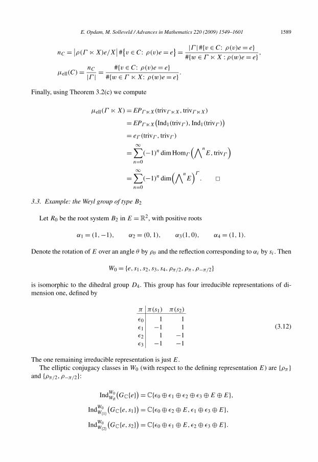
E. Opdam, M. Solleveld / Advances in Mathematics 220 (2009) 1549–1601 1589
nC = ∣∣ρ(Γ � X)e/X∣∣#{v ∈ C: ρ(v)e = e
} = |Γ | #{v ∈ C: ρ(v)e = e}#{w ∈ Γ � X : ρ(w)e = e} ,
μell(C) = nC
|Γ | = #{v ∈ C: ρ(v)e = e}#{w ∈ Γ � X: ρ(w)e = e} .
Finally, using Theorem 3.2(c) we compute
μell(Γ � X) = EPΓ �X(trivΓ �X, trivΓ �X)
= EPΓ �X
(Ind1(trivΓ ), Ind1(trivΓ )
)= eΓ (trivΓ , trivΓ )
=∞∑
n=0
(−1)n dim HomΓ
(∧nE, trivΓ
)
=∞∑
n=0
(−1)n dim(∧n
E)Γ
. �
3.3. Example: the Weyl group of type B2
Let R0 be the root system B2 in E = R2, with positive roots
α1 = (1, −1), α2 = (0,1), α3(1,0), α4 = (1,1).
Denote the rotation of E over an angle θ by ρθ and the reflection corresponding to αi by si . Then
W0 = {e, s1, s2, s3, s4, ρπ/2, ρπ ,ρ−π/2 }
is isomorphic to the dihedral group D4. This group has four irreducible representations of di-mension one, defined by
π π(s1) π(s2)
ε0 1 1ε1 −1 1ε2 1 −1ε3 −1 −1
(3.12)
The one remaining irreducible representation is just E.The elliptic conjugacy classes in W0 (with respect to the defining representation E) are {ρπ }
and {ρπ/2, ρ−π/2 }:
IndW0W∅(GC{e}) = C{ε0 ⊕ ε1 ⊕ ε2 ⊕ ε3 ⊕ E ⊕ E},
IndW0W{1}(GC{e, s1 }) = C{ε0 ⊕ ε2 ⊕ E,ε1 ⊕ ε3 ⊕ E},
IndW0(GC{e, s2 }) = C{ε0 ⊕ ε1 ⊕ E,ε2 ⊕ ε3 ⊕ E}.
W{2}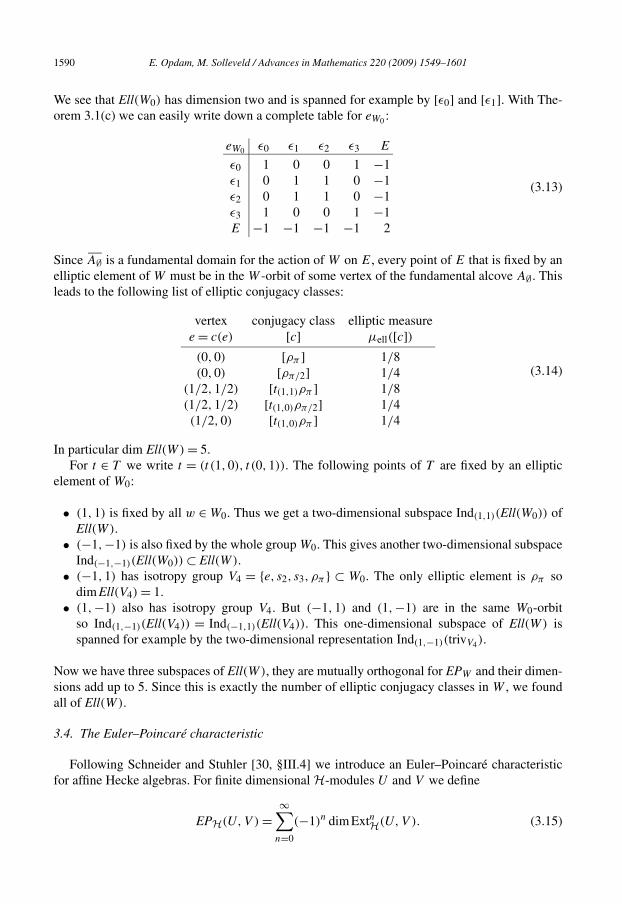
1590 E. Opdam, M. Solleveld / Advances in Mathematics 220 (2009) 1549–1601
We see that Ell(W0) has dimension two and is spanned for example by [ε0 ] and [ε1 ]. With The-orem 3.1(c) we can easily write down a complete table for eW0 :
eW0 ε0 ε1 ε2 ε3 E
ε0 1 0 0 1 −1ε1 0 1 1 0 −1ε2 0 1 1 0 −1ε3 1 0 0 1 −1E −1 −1 −1 −1 2
(3.13)
Since A∅ is a fundamental domain for the action of W on E, every point of E that is fixed by anelliptic element of W must be in the W -orbit of some vertex of the fundamental alcove A∅. Thisleads to the following list of elliptic conjugacy classes:
vertex conjugacy class elliptic measuree = c(e) [c] μell([c])(0,0) [ρπ ] 1/8(0,0) [ρπ/2 ] 1/4
(1/2,1/2) [t(1,1)ρπ ] 1/8(1/2,1/2) [t(1,0)ρπ/2 ] 1/4(1/2,0) [t(1,0)ρπ ] 1/4
(3.14)
In particular dim Ell(W) = 5.For t ∈ T we write t = (t (1,0), t (0,1)). The following points of T are fixed by an elliptic
element of W0:
• (1,1) is fixed by all w ∈ W0. Thus we get a two-dimensional subspace Ind(1,1)(Ell(W0)) ofEll(W).
• (−1, −1) is also fixed by the whole group W0. This gives another two-dimensional subspaceInd(−1,−1)(Ell(W0)) ⊂ Ell(W).
• (−1,1) has isotropy group V4 = {e, s2, s3, ρπ } ⊂ W0. The only elliptic element is ρπ sodim Ell(V4) = 1.
• (1, −1) also has isotropy group V4. But (−1,1) and (1, −1) are in the same W0-orbitso Ind(1,−1)(Ell(V4)) = Ind(−1,1)(Ell(V4)). This one-dimensional subspace of Ell(W) isspanned for example by the two-dimensional representation Ind(1,−1)(trivV4).
Now we have three subspaces of Ell(W), they are mutually orthogonal for EPW and their dimen-sions add up to 5. Since this is exactly the number of elliptic conjugacy classes in W , we foundall of Ell(W).
3.4. The Euler–Poincaré characteristic
Following Schneider and Stuhler [30, §III.4] we introduce an Euler–Poincaré characteristicfor affine Hecke algebras. For finite dimensional H-modules U and V we define
EPH(U,V ) =∞∑
(−1)n dim ExtnH(U,V ). (3.15)
n=0
E. Opdam, M. Solleveld / Advances in Mathematics 220 (2009) 1549–1601 1591
By Proposition 2.4 the sum is actually finite, so this is well defined. With standard homologicalalgebra (see for instance [6]) one can show that this extends to a bilinear pairing on G(H). Reeder[29] studied this pairing for affine Hecke algebras with equal parameters, via p-adic groups.
Proposition 3.4.
(a) Let I ⊂ F0 be a proper subset of simple roots and let V ∈ Modfin(H(RI , qI )). Then
EPH(U, IndH
H(RI ,qI )V) = 0 ∀U ∈ Modfin(H).
(b) If the root datum R is not semisimple then EPH ≡ 0.
Proof. This result is the translation of [30, Lemma III.4.18.ii] to affine Hecke algebras. Theproof is similar and based on an argument due to Kazhdan.
We may assume that (π,V ) is irreducible with Z(H(RI , qI ))-character WI t ∈ T/WI .If W0t is not an Z(H)-weight of U then ExtH
n (U, IndHH(RI ,qI )
V ) = 0, so certainly EPH(U,
IndHH(RI ,qI )
V ) = 0. Therefore we may also assume that U is irreducible with Z(H)-characterW0t ∈ T/W0.
Recall the groups G ⊂ W0(R) from (1.4). Objects constructed from R will be denoted by thesame symbol as the corresponding objects for R, but with additional tilde. Like on page 1561we have the fundamental alcove A∅, the subgroup Ω ⊂ W(R) of elements of length zero, a facetf of A∅, and its stabilizer Ω
f. Let Fn be a set of representatives for the action of Ω on these
facets. We abbreviate
mt = #{g ∈ G: gW0t = W0t },U = IndH(R,q)
H(R,q)(U).
From (2.24), Corollary 2.3(a) and the Euler–Poincaré principle we deduce that
mtEPH(U, IndH
H(RI ,qI )V)
= EPH(U, IndH(R,q)
H(RI ,qI )V)
= EPH(R,q)
(U , IndH(R,q)
H(RI ,qI )V)
=∞∑
n=0
(−1)n dim ExtnH(R,q)
(U , IndH(R,q)
H(RI ,qI )V)
=rk(X)∑n=0
(−1)n dim(HomH(R,q)
(Pn(U)Ω , IndH(R,q)
H(RI ,qI )V))
=rk(X)∑n=0
(−1)n dim
(HomH(R,q)
(⊕˜
IndH(R,q)
H(R,f ,q)(U ⊗ ε
f), IndH(R,q)
H(RI ,qI )V
))
f ∈ Fn
1592 E. Opdam, M. Solleveld / Advances in Mathematics 220 (2009) 1549–1601
=rk(X)∑n=0
(−1)n dim
(⊕f ∈ Fn
HomH(R,f ,q)
(U ⊗ ε
f, IndH(R,q)
H(RI ,qI )V))
=rk(X)∑n=0
(−1)n∑
f ∈ Fn
dim HomH(R,f ,q)
(U ⊗ ε
f, IndH(R,q)
H(RI ,qI )V). (3.16)
Because V is irreducible there exist a H(RI , qI )-representation (π1,V ) and a Z(W(RI ))-character t1, such that
(π,V ) = (π1 ◦ φt1 ,V )
with φt1 as in (1.8). Note that Z(W(RI )) = (I ∨)⊥ ∩ X = 0 because I = F0. Let t2 be an arbitraryZ(W(RI ))-character and consider the integer
dim HomH(R,f ,q)
(U ⊗ ε
f, IndH(R,q)
H(RI ,qI )(π1 ◦ φt2 ,V )
).
According to Lemma 1.4 H(R, f , q) is a finite dimensional semisimple algebra. Therefore theabove integer is invariant under continuous deformations of t2, and hence independent of t2. Pick
t2 such that the central character of IndH(R,q)
H(RI ,qI )(π1 ◦ φt2 ,V ) is not W0(R)t ∈ T/W0(R). Then
0 = mtEPH(U, IndH(R,q)
H(RI ,qI )(π1 ◦ φt2 ,V )
)=
rk(X)∑n=0
(−1)n∑
f ∈ Fn
dim HomH(R,f ,q)
(U ⊗ ε
f, IndH(R,q)
H(RI ,qI )(π1 ◦ φt2 ,V )
)
=rk(X)∑n=0
(−1)n∑
f ∈ Fn
dim HomH(R,f ,q)
(U ⊗ ε
f, IndH(R,q)
H(RI ,qI )(π1 ◦ φt1 ,V )
)= mtEPH
(U, IndH
H(RI ,qI )(π,V )
). (3.17)
To prove (b) we suppose that R is not semisimple and that U ′,V ′ ∈ Modfin(H). We have to showthat
EPH(U ′,V ′) = 0.
We may assume that U ′ and V ′ admit the same central character W0t . From the proof of part (a)we see that
mtEPH(U ′,V ′) = EPH(R,q)
(IndH(R,q)
H U ′, IndH(R,q)
H V ′) = 0. �We can use the scaling maps
σε : Modfin(
H(R, q)) → Modfin
(H(
R, qε))
from Theorem 1.7 to relate EPH to EPW .
E. Opdam, M. Solleveld / Advances in Mathematics 220 (2009) 1549–1601 1593
Theorem 3.5.
(a) The pairing EPH is symmetric and positive semidefinite.(b) If U,V ∈ Modfin(H) then
EPH(U,V ) = EPH(R,qε)
(σε(U), σε(V )
) ∀ε ∈ [−1,1].
Proof. In view of Proposition 3.4(b) we may assume that R is semisimple. For every ε ∈ [−1,1]Theorem 1.7 gives us the H(R, qε)-representations
σε(ρ,U) = (ρε,U) and σε(π,V ) = (πε,V ).
As a vector space H(R, f, qε) is just C[Wf � Ωf ]. As an algebra it is semisimple and themultiplication varies continuously with ε, so by Tits’ deformation theorem it is independent of ε.Furthermore for any w ∈ Wf � Ωf the maps
ε �→ ρε(Nw) and ε �→ πε(Nw)
are continuous. In view of (3.16) this implies that
EPH(R,qε)
(σε(U), σε(V )
)depends continuously on ε. But this expression is integer-valued, so it is actually independentof ε. In particular
EPH(U,V ) = EPW
(σ0(U), σ0(V )
). (3.18)
Now Theorem 3.2(b) assures that EPH is symmetric and positive semidefinite. �For semisimple root data we can also compute the Euler–Poincaré characteristic in another
way, as the character value of a certain index function.According to Lemma 1.4 the algebra H(R, f, q) is finite dimensional and semisimple, for
all facets f of the fundamental alcove A∅. In particular the collection Irr(H(R, f, q)) of irre-ducible representations is finite. Let eσ ∈ H(R, f, q) denote the primitive central idempotentcorresponding to an irreducible H(R, f, q)-module σ . For U ∈ Mod(H(R, f, q)) let [U : σ ] bethe multiplicity of σ in U .
In the spirit of Kottwitz [18, §2], Schneider and Stuhler [30, III.4] we define an Euler–Poincaréfunction
f UEP :=
∑f ⊂A∅
(−1)dimf
[Ω : Ωf ]∑
σ ∈Irr(H(R,f,q))
[U ⊗ εf : σ ]dimσ
eσ . (3.19)
Proposition 3.6. Let R be a semisimple root datum and U,V ∈ Modfin(H). Then
EPH(U,V ) = χV
(f U
EP
).
1594 E. Opdam, M. Solleveld / Advances in Mathematics 220 (2009) 1549–1601
Proof. Exactly like in (3.16) we can calculate that
EPH(U,V ) =rk(X)∑n=0
(−1)n dim HomH(Pn(U)Ω,V
)
=rk(X)∑n=0
∑f : dimf =n
(−1)n
[Ω : Ωf ] dim HomH(R,f,q)(U ⊗ εf ,V )
=∑
f ⊂A∅
(−1)dimf
[Ω : Ωf ]∑
σ ∈Irr(H(R,f,q))
[U ⊗ εf : σ ] [V : σ ]
=∑
f ⊂A∅
(−1)dimf
[Ω : Ωf ]∑
σ ∈Irr(H(R,f,q))
[U ⊗ εf : σ ]dimσ
χV (eσ )
= χV
(f U
EP
). �
We will use this result in [28] to show that the Plancherel measure of a discrete series repre-sentation is a rational function in q , with rational coefficients.
3.5. Extensions of tempered modules
We apply the results of Section 2 to relate the bornological Tor and Ext functors over H withthose over S . That is more interesting than it looks at first sight, because S is not flat over H(unless q ≡ 1).
Corollary 3.7. Take n ∈ N.
(a) For all Ub,Vb ∈ Modbor(S) the inclusion H → S induces isomorphisms
TorHn (S,Vb) ∼= TorS
n (S,Vb) ∼={
Vb if n = 0,
0 if n > 0,
ExtnH(Ub,Vb) ∼= ExtnS (Ub,Vb).
(b) For all finite dimensional tempered H-modules U and V there is a natural isomorphismExtnH(U,V ) ∼= ExtnS (U,V ).
(c) EPH(U,V ) = EPS (U,V ).
Proof. (a) follows directly from Theorems 2.9(a) and A.1.(b) In this setting the bornological functor ExtH
n agrees with its purely algebraic counterpart,as discussed in Appendix A. The same holds for ExtS
n , because the resolution from Corollary 2.7consists of S -modules that are projective in both the algebraic and the bornological sense. Hence(b) is a special case of (a).
However, for semisimple root data this can be proved more directly, without the use ofbornological techniques. Namely, we can simply compare the projective resolutions from Corol-laries 2.3(a) and 2.7(a). If we use these to compute the Ext-groups and we apply Frobenius
E. Opdam, M. Solleveld / Advances in Mathematics 220 (2009) 1549–1601 1595
reciprocity, then we see that ExtnH(U,V ) and ExtnS (U,V ) are the homologies of isomorphicdifferential complexes. See also the remark at the end of Section 2.3.
(c) is a trivial consequence of (b). �We remark that the corresponding results for reductive p-adic groups were proved in [23, §7]
and [31, §9]. These proofs are much more involved however, in particular no shortcut like theone described in our proof seems available.
Notice that we have to take the derived functors with respect to bornological tensor productsand bounded maps, if we want to get Corollary 3.7(a) for infinite dimensional modules. If wewould work purely algebraically this would already fail for U = V = S .
The main use of Corollary 3.7 is the next theorem.
Theorem 3.8. Suppose that U and V are irreducible tempered H-modules. If U or V belongs tothe discrete series then
ExtnH(U,V ) ∼={
C if U ∼= V and n = 0,
0 otherwise.
Proof. The assertion for n = 0 follows directly from Schur’s lemma and the general isomor-phism Ext0 ∼= Hom.
Let δ be a discrete series representation of H. According to [9, Corollary 3.13] EndC(δ) is adirect summand of S , as algebras. Therefore δ is both injective and projective as an S -module.Using Corollary 3.7(b) we find that for any tempered H-module V and any n > 0
ExtnH(V , δ) = ExtnS (V , δ) = 0 (3.20)
because δ is injective, and
ExtnH(δ,V ) = ExtnS (δ,V ) = 0 (3.21)
because δ is projective. �Let us introduce the space of “elliptic trace functions”
Ell(H) := GC(H)/ ∑
I ⊂F0, I⊥ =0
IndHH(RI ,qI )
GC
(H(
RI , qI))
, (3.22)
where I ⊥ = {y ∈ Y : 〈α,y〉 = 0 ∀α ∈ I }. Notice that this space is zero whenever R is notsemisimple. From Proposition 3.4 and Theorem 3.5 we see that the Euler–Poincaré character-istic induces a semidefinite Hermitian form on Ell(H):
EPH(λ[U ],μ[V ]) := λμEPH(U,V ), U,V ∈ Modfin(H), λ,μ ∈ C.
Proposition 3.9.
(a) The scaling map σ0 induces a linear map Ell(H) → Ell(W) which is an isometry with respectto the (semidefinite) Hermitian forms EPH and EPW .
(b) The number of inequivalent discrete series representations of H is at most the number ofelliptic conjugacy classes in W .
1596 E. Opdam, M. Solleveld / Advances in Mathematics 220 (2009) 1549–1601
Proof. (a) follows directly from Theorem 3.5(b).(b) According to Theorem 3.8 the inequivalent discrete series representations form an or-
thonormal set in Ell(H). By part (a) the same holds for their images in Ell(W). From Theo-rem 3.2(a) we know that the dimension of Ell(W) is precisely the number of elliptic conjugacyclasses in W . �Remark. A lower bound for the number of discrete series representations can be obtained fromcounting their central characters. In turns out that for the crucial irreducible non-simply lacedcases C
(1)n , F4 and G2 this lower bound equals the above upper bound, for generic parameters.
We will exploit this in [28] to give a classification of the irreducible discrete series characters forany irreducible non-simply laced affine Hecke algebra, with arbitrary positive parameters.
Example. Let R0 = A1 = {1, −1} = {±α} and X = Z. Then W0 = {e, sα∨ } and W is generatedby sα∨ and s1+α∨ . Take a label function such that q(sα∨ ) = q(s1+α∨ ) = q > 1. The affine Heckealgebra H = H(A1, q) has a unique discrete series representation called the Steinberg represen-tation. It has dimension one and is defined simply by
St(Nw) = (−1)�(w)q(w)−1/2 = (−q−1/2)�(w).
On the other hand we have the “trivial” H-representation, defined by
trivH(Nw) = q(w)1/2 = q�(w)/2.
It is unitary but not tempered. From Theorem 3.8 we see that
EPH(St,St) = 1,
but is not immediately clear how many extensions of St by trivH there are. There certainly is anextension
0 ← St ← IndHA (φq−1) ← trivH ← 0, (3.23)
so [IndHA (φq−1)] = [St] + [trivH ] in G(H). Therefore
EPH(St, trivH) = EPH(St, [trivH ] − [IndH
A (φq−1)])
= EPH(St, −[St]) = −1.
From Corollary 2.3(d) we know that the cohomological dimension of Mod(H) is 1, so in partic-ular
ExtnH(St, trivH) = 0 for n > 1.
Therefore (3.23) is up to a scalar factor the only nontrivial extension of St by trivH.
E. Opdam, M. Solleveld / Advances in Mathematics 220 (2009) 1549–1601 1597
Acknowledgments
This research originated from joint work of Mark Reeder and the first author. We are alsograteful to Ralf Meyer and Henk Pijls for some useful advice.
A part of this paper was written while the authors were guests of the Max Planck Institut fürMathematik and the Hausdorff Research Institute for Mathematics, both in Bonn. We thank theseinstitutions for their hospitality.
Appendix A. Bornological algebras
In Section 2 we induce several modules from H to S . From an analytical point of view thisoperation is trivial for finite dimensional modules, since in that case all involved tensor productsare purely algebraic. However for infinite dimensional modules we have to take the topologyinto account. For Fréchet S -modules we can use the complete projective tensor product. But fortensor products over H this is problematic, because there is no canonical topology on H.
Consider for example the trivial one-dimensional root datum (Z, ∅,Z, ∅). Then
H = C[Z] ∼= O(C×), S = S(Z) ∼= C∞(S1).For t ∈ S1 the ideal
Jt := {f ∈ C∞(S1): f (t) = 0} ⊂ C∞(S1)
is generated by Jt ∩ O(C×). It follows that for any finite dimensional S(Z)-module V we have
S(Z) ⊗C[Z] V ∼= S(Z) ⊗S(Z) V = V.
This property does not readily generalize to infinite dimensional modules, for example
S(Z) ⊗C[Z] S(Z) ∼= S(Z) ⊗S(Z) S(Z) = S(Z).
The right technique to fix this is bornology. On many vector spaces bornological and topologicalanalysis are equivalent, but bornologies combine well with homological algebra in larger classes.Bornologies are not so well known, so we provide a brief introduction. See also [21,22].
A bornology on a complex vector space is a certain collection of subsets that are calledbounded. This collection has to satisfy some axioms that generalize obvious properties ofbounded sets in Banach spaces. A morphism of bornological vector spaces is a linear map thatsends bounded sets to bounded sets. There is a natural notion of completeness of bornologicalvector spaces, similar to that of completeness of locally convex spaces.
On any vector space V we can define a more or less trivial bornology, the fine bornology.A subset X ⊂ V belongs to this bornology if and only if X is a bounded (in the usual sense)subset of some finite dimensional subspace of V . In this case V is bornologically complete andany linear map from V to another bornological vector space is bounded. By default we equipvector spaces with a countable basis with the fine bornology.
More interestingly, if V is a complete topological vector space (e.g. a Fréchet space) wecan define the precompact bornology on V as follows. We call X ⊂ V bounded if and only if itsclosure X is compact. Under these assumptions V is bornologically complete and any continuous
1598 E. Opdam, M. Solleveld / Advances in Mathematics 220 (2009) 1549–1601
map between such vector spaces is bounded. Conversely, any bounded linear map between twoFréchet spaces with the precompact bornology is continuous [21, Lemma 2.2].
The category of bornological vector spaces is not abelian, but it does have enough injectiveand projective objects. It also possesses inductive and projective limits.
Let V be a bornological vector space and Endbor(V ) the algebra of bounded linear mapsV → V . A subset L ⊂ Endbor(V ) is equibounded if L(X) := {l(x): l ∈ L, x ∈ X} is boundedfor any bounded set X ⊂ V . This gives Endbor(V ) the structure of a bornological algebra.
Let A be a unital bornological algebra. By definition a bornological A-module structure onV is the same as a bounded bilinear map A × V → V , or as a bounded algebra homomorphismA → Endbor(V ). Let Modbor(A) be the category of bornological A-modules.
The A-balanced completed bornological tensor product ⊗A is defined by the following uni-versal property. Bounded linear maps V1 ⊗A V2 → V3 with V3 complete correspond bijectivelyto bounded bilinear maps b : V1 × V2 → V3 that satisfy b(v1a, v2) = b(v1, av2).
In case V1,V2 and A have the fine bornology this is just the algebraic tensor product over A.On the other hand, if V1,V2 and A are Fréchet spaces with the precompact bornology, then thisagrees with the completed projective tensor product over A.
By definition a sequence
0 → V1 → V2 → V3 → 0
in Modbor(A) is a bornological extension if the maps are bounded A-module homomorphismsand the sequence is split exact in the category of bornological vector spaces. We call a differ-ential complex of bornological A-modules exact if it admits a bounded C-linear contraction.These notions of extensions and exactness make Modbor(A) into an exact category, whose de-rived category we denote by Derbor(A). Let ⊗L
A and RHomA denote the total derived functorsof ⊗A and HomA. Thus U ⊗L
A V is an object of Derbor(A) whose homology is TorA∗ (U,V ), andthe (co)homology of RHomA(U,V ) is Ext∗
A(U,V ). However, the total derived functors containsomewhat more information, as the passage to homology forgets the bornological properties ofthese differential complexes.
Suppose that A,U and V have the fine bornology. Then the bornological functors ⊗A andHomA agree with their algebraic counterparts. Hence TorAn (U,V ) and ExtnA(U,V ) are the samein the algebraic and the bornological sense.
Let f : A → B be a morphism of unital complete bornological algebras and
0 ← A ← P0 ← P1 ← · · ·a resolution of A by projective A ⊗ Aop-modules.
Theorem A.1. (See [22, Theorem 35].) The following are equivalent:
(1) B ⊗A P∗ ⊗A B is a projective B ⊗ Bop-module resolution of B .(2) (f ∗B) ⊗L
A (f ∗B) → B ⊗L
B B (∼= B) is an isomorphism.
(3) (f ∗U) ⊗L
A (f ∗V ) → U ⊗L
B V is an isomorphism ∀U ∈ Modbor(Bop), V ∈ Modbor(B).
(4) RHomB(U,V ) → RHomA(f ∗U,f ∗V ) is an isomorphism ∀U,V ∈ Modbor(B).(5) The functor f ∗ : Derbor(B) → Derbor(A) is fully faithful.
We call f isocohomological if these conditions hold.
E. Opdam, M. Solleveld / Advances in Mathematics 220 (2009) 1549–1601 1599
Direct consequences of conditions (3) and (4) are
TorB∗ (U,V ) ∼= TorA∗ (f ∗U,f ∗V ),
Ext∗B(U,V ) ∼= Ext∗
A(f ∗U,f ∗V ), (A.1)
where we mean the derived functors in the bornological category.We equip H with the fine bornology and let Modbor(H) be the category of all bornologi-
cal H-modules. Notice that any H-module can be made bornological by endowing it with thefine bornology. This identifies Mod(H) with a full subcategory of Modbor(H). An H-module isbornologically projective if and only if it is algebraically projective, namely if and only if it is adirect summand of an (algebraically) free H-module. So as long as we are working in a purelyalgebraic setting the bornological structure does not give much extra, but neither is it a restriction.
We endow S with the precompact bornology, so that any finite dimensional S -module isbornological. We denote the category of all bornological S -modules by Modbor(S). Probablythere exist S -modules that do not admit the structure of a bornological S -module, but they seemto be rather far-fetched. We note that a projective object of Modbor(S) is usually not a projectiveS -module in the algebraic sense, rather a completion of the latter.
A bornological H-module (π,V ) is called tempered if it extends to S , that is, if the followingequivalent conditions hold:
(1) π extends to a bounded algebra homomorphism S → Endbor(V ),(2) π induces a bounded bilinear map S × V → V .
A (sub-)linear functional f : H → C is tempered if there exist C,N ∈ (0, ∞) such that∣∣f (Nw)∣∣� C
(1 + N (w)
)N ∀w ∈ W.
The collection of all tempered linear functionals is the continuous dual space of S(R, q).
Proposition A.2. Let V be a Fréchet space endowed with the precompact bornology. An H-module (π,V ) is bornological if and only if π(h) : V → V is continuous ∀h ∈ H. Moreover it istempered if and only if the following equivalent conditions hold:
(3) π induces a jointly continuous map S × V → V ,(4) π induces a separately continuous map S × V → V ,(5) for every v ∈ V and every continuous seminorm p on V the sublinear functional
H → [0, ∞) : h �→ p(π(h)v
)is tempered,
(6) for every v ∈ V and every f ∈ V ∗ the linear functional
H → C : h �→ f(π(h)v
)is tempered.
In particular the category ModFré(S) of continuous Fréchet S -modules is a full subcategory ofModbor(S).
1600 E. Opdam, M. Solleveld / Advances in Mathematics 220 (2009) 1549–1601
Proof. We already noted that π(h) : V → V is continuous if and only if it is bounded. Since Hcarries the fine bornology this is equivalent to the first assertion.
For the same reason ModFre(S) forms a full subcategory of Modbor(S).It is clear that condition (3) implies the other five. Conversely (3) follows from (2) by [21,
Lemma 2.2] and from (4) by the Banach–Steinhaus theorem.If f ∈ V ∗ then |f | is a continuous seminorm on V , so (5) implies (6).Finally we show that (6) implies (4). Endow H with the induced topology from S and fix
v ∈ V . By assumption the linear map
H → V : h �→ π(h)v (A.2)
is continuous for the weak topology on V . Since V is Fréchet (A.2) is also continuous for themetric topology on V [17, 21.4.i]. Hence (A.2) extends continuously to the metric completion Sof H.
Now we fix h = ∑w∈W hwNw ∈ S and we write hn = ∑
w: N (w)�n hwNw . We assumed thatV is a Fréchet H-module, so (π(hn))
∞n=1 is a sequence of continuous linear operators on V . We
just showed that for fixed v ∈ V the sequence (π(hn)v)∞n=1 converges to π(h)v. The Banach–
Steinhaus theorem (see e.g. [17, pp. 104–105]) assures that π(h) is continuous.We conclude that (h, v) �→ π(h)v is separately continuous. �
References
[1] J. Arthur, On elliptic tempered characters, Acta Math. 171 (1993) 73–138.[2] R. Bezrukavnitkov, Homological properties of representations of p-adic groups related to geometry of the group at
infinity, PhD thesis, Tel Aviv University, 1998.[3] F. Bruhat, J. Tits, Groupes réductifs sur un corps local I. Données radicielles valuées, Publ. Math. Inst. Hautes
Études Sci. 41 (1972) 5–251.[4] C.J. Bushnell, P.C. Kutzko, Smooth representations of reductive p-adic groups: Structure theory via types, Proc.
London Math. Soc. 77 (3) (1998) 582–634.[5] C.J. Bushnell, P.C. Kutzko, Types in reductive p-adic groups: The Hecke algebra of a cover, Proc. Amer. Math.
Soc. 129 (2) (2001) 601–607.[6] H. Cartan, S. Eilenberg, Homological Algebra, Princeton University Press, 1956.[7] W. Casselman, Introduction to the theory of admissible representations of p-adic reductive groups, draft, 1995.[8] A.H. Clifford, Representations induced in an invariant subgroup, Ann. of Math. 38 (1937) 533–550.[9] P. Delorme, E.M. Opdam, The Schwartz algebra of an affine Hecke algebra, J. Reine Angew. Math. 625 (2008)
59–114.[10] J. Dixmier, Les C∗ -algèbres et leurs représentations, Cahiers Scientifiques, vol. 29, Gauthier–Villars Éditeur, Paris,
1969.[11] G.J. Heckman, E.M. Opdam, Harmonic analysis for affine Hecke algebras, in: Current Developments in Mathemat-
ics, International Press, 1997, pp. 37–60.[12] R.B. Howlett, G.I. Lehrer, Representations of generic algebras and finite groups of Lie type, Trans. Amer. Math.
Soc. 280 (2) (1983) 753–779.[13] J.E. Humphreys, Reflection Groups and Coxeter Groups, Cambridge Stud. Adv. Math., vol. 29, Cambridge Univer-
sity Press, 1990.[14] N. Iwahori, H. Matsumoto, On some Bruhat decomposition and the structure, of the Hecke rings of the p-adic
Chevalley groups, Inst. Hautes Études Sci. Publ. Math. 25 (1965) 5–48.[15] S.-I. Kato, Duality for representations of a Hecke algebra, Proc. Amer. Math. Soc. 119 (3) (1993) 941–946.[16] D. Kazhdan, Cuspidal geometry of p-adic groups, J. Anal. Math. 67 (1986) 1–36.[17] J.L. Kelley, I. Namioka, Linear Topological Spaces, Grad. Texts in Math., vol. 36, Van Nostrand, 1963.[18] R.E. Kottwitz, Tamagawa numbers, Ann. of Math. 127 (3) (1988) 629–646.[19] G. Lusztig, Affine Hecke algebras and their graded version, J. Amer. Math. Soc. 2 (3) (1989) 599–635.[20] G. Lusztig, Classification of unipotent representations of simple p-adic groups, Int. Math. Res. Not. 11 (1995)
517–589.
E. Opdam, M. Solleveld / Advances in Mathematics 220 (2009) 1549–1601 1601
[21] R. Meyer, Bornological versus topological analysis in metrizable spaces, in: Contemp. Math., vol. 363, 2004,pp. 249–278.
[22] R. Meyer, Embeddings of derived categories of bornological modules, arXiv: math.FA/0410596, 2004.[23] R. Meyer, Homological algebra for Schwartz algebras of reductive p-adic groups, in: Noncommutative Geometry
and Number Theory, in: Aspects Math., vol. E37, Vieweg Verlag, 2006, pp. 263–300.[24] L. Morris, Tamely ramified intertwining algebras, Invent. Math. 114 (1993) 233–274.[25] L. Morris, Level zero G-types, Compos. Math. 118 (2) (1999) 135–157.[26] E.M. Opdam, On the spectral decomposition of affine Hecke algebras, J. Inst. Math. Jussieu 3 (4) (2004) 531–648.[27] E.M. Opdam, Hecke algebras and harmonic analysis, in: Proceedings of the International Congress of Mathemati-
cians, vol. II, Madrid, August 22–30, 2006, EMS Publ. House, 2006, pp. 1227–1259.[28] E.M. Opdam, M.S. Solleveld, Discrete series characters for affine Hecke algebras and their formal dimensions,
arXiv: 0804.0026, 2008.[29] M. Reeder, Euler–Poincaré pairings and elliptic representations of Weyl groups and p-adic groups, Compos.
Math. 129 (2001) 149–181.[30] P. Schneider, U. Stuhler, Representation theory and sheaves on the Bruhat–Tits building, Publ. Math. Inst. Hautes
Études Sci. 85 (1997) 97–191.[31] P. Schneider, E.-W. Zink, The algebraic theory of tempered representations of p-adic groups. Part II: Projective
generators, Geom. Funct. Anal. 17 (6) (2008) 2018–2065.[32] G. Skandalis, Progrès récents sur la conjecture de Baum–Connes. Contribution de Vincent Lafforgue,
Astérisque 276 (2002).[33] M.S. Solleveld, Periodic cyclic homology of affine Hecke algebras, PhD thesis, Universiteit van Amsterdam, 2007.[34] M.-F. Vignéras, Extensions between irreducible representations of p-adic GL(n), Pacific J. Math. 181 (3) (1997)
349–357.[35] J.-L. Waldspurger, Produit scalaire elliptique, Adv. Math. 210 (2) (2007) 607–634.
![FORMAL HECKE ALGEBRAS AND ALGEBRAIC ORIENTED … · arXiv:1208.4114v4 [math.RA] 27 Mar 2014 FORMAL HECKE ALGEBRAS AND ALGEBRAIC ORIENTED COHOMOLOGY THEORIES ALEX HOFFNUNG, JOSE MALAG´](https://img.pdfslide.us/doc/110x75/5f49e94c4ae1e674ed145844/formal-hecke-algebras-and-algebraic-oriented-arxiv12084114v4-mathra-27-mar.jpg)
![Automorphisms of Generic Iwahori-Hecke Algebras and Integral … · 2017-02-05 · Automorphisms of Generic Iwahori]Hecke Algebras and Integral Group Rings of Finite Coxeter Groups*](https://img.pdfslide.us/doc/110x75/5f6ff7728095716e045b5abf/automorphisms-of-generic-iwahori-hecke-algebras-and-integral-2017-02-05-automorphisms.jpg)

![Decomposition Numbers for Generic Iwahori-Hecke Algebras ... · Generic Iwahori]Hecke algebras of the classical series A, B, D and of the exceptional types G 24 6 7 8, F, E, E, E,](https://img.pdfslide.us/doc/110x75/5f7008b7e53a70183508680f/decomposition-numbers-for-generic-iwahori-hecke-algebras-generic-iwahorihecke.jpg)


![CONSTRUCTING REPRESENTATIONS OF HECKE ...Constructing representations of Hecke algebras for complex reflection groups irreducible. Then it is known by [4, remark 12.4] that, except](https://img.pdfslide.us/doc/110x75/5ed5a55693303d72c21d1699/constructing-representations-of-hecke-constructing-representations-of-hecke.jpg)