Embed Size (px)
Citation preview


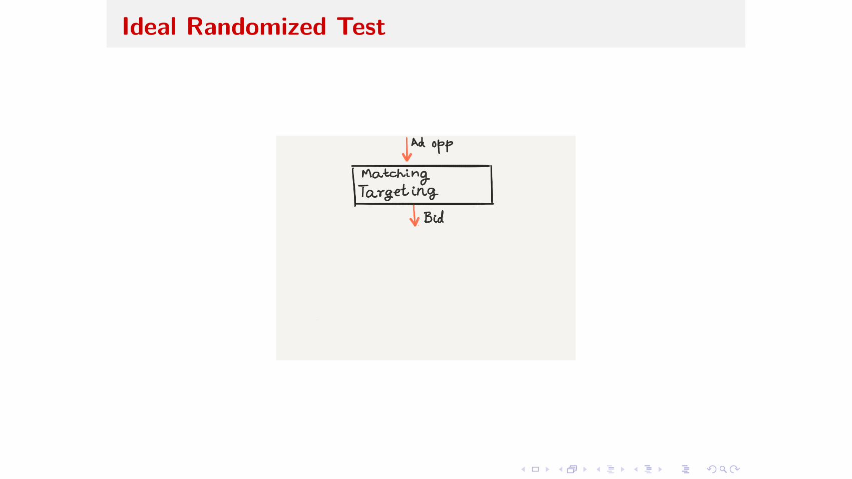
I listen to ~ 100 Bln ad opportunities daily
I respond with optimal bids within milliseconds
I petabytes of data (ad impressions, visits, clicks, conversions)

I listen to ~ 100 Bln ad opportunities daily
I respond with optimal bids within milliseconds
I petabytes of data (ad impressions, visits, clicks, conversions)

I listen to ~ 100 Bln ad opportunities daily
I respond with optimal bids within milliseconds
I petabytes of data (ad impressions, visits, clicks, conversions)

I listen to ~ 100 Bln ad opportunities daily
I respond with optimal bids within milliseconds
I petabytes of data (ad impressions, visits, clicks, conversions)

Predicting user response to ads is a Machine-Learning problem.
but quantifying impact of ad-exposure is a Measurement probem.

Predicting user response to ads is a Machine-Learning problem.but quantifying impact of ad-exposure is a Measurement probem.

Spark: existing vs simulated data
Most Spark applications process existing big data-sets.
Today we’re talking about analyzing simulated big data

Spark: existing vs simulated data
Most Spark applications process existing big data-sets.Today we’re talking about analyzing simulated big data
Key Conceptual Take-aways
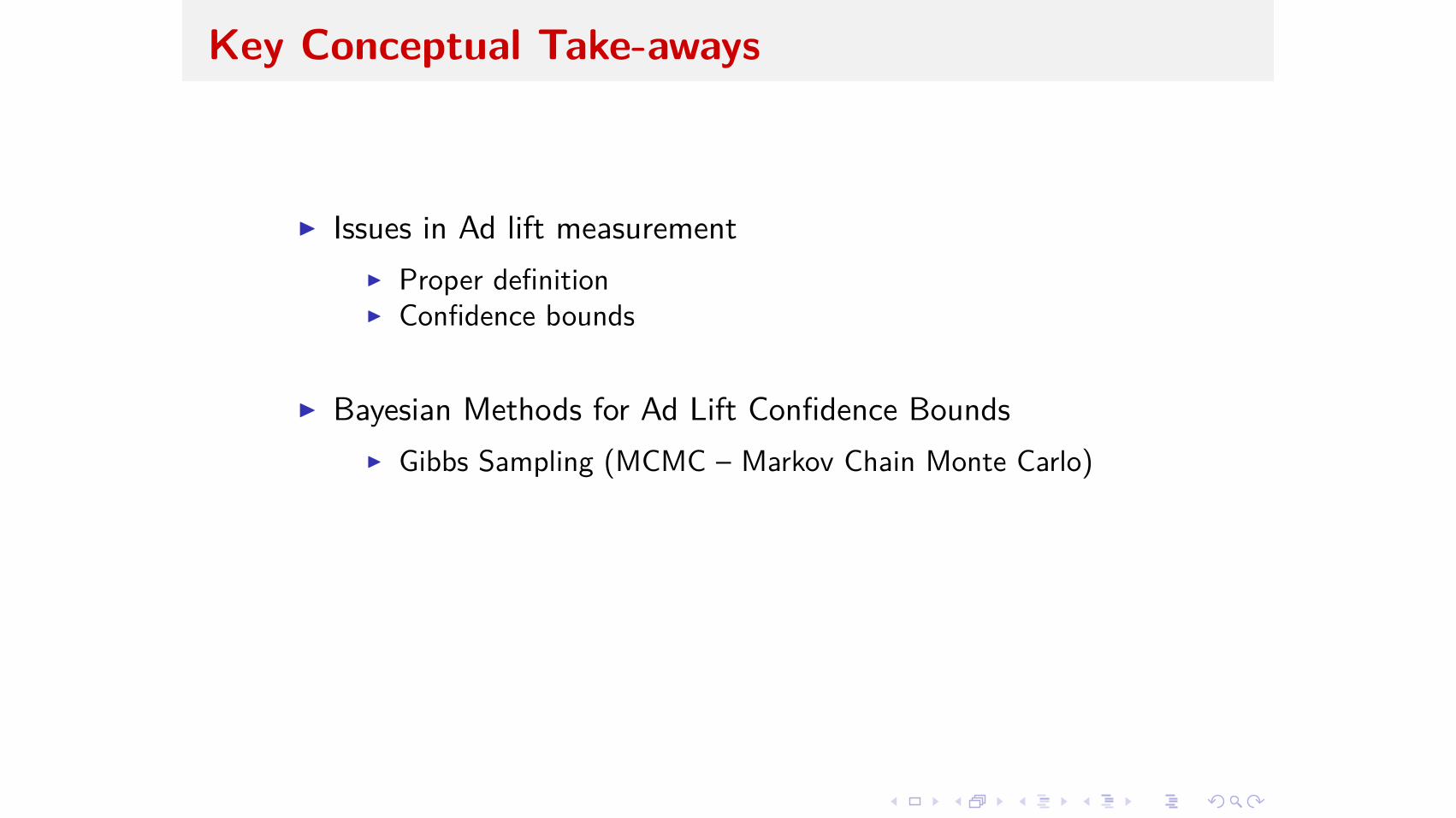
I Issues in Ad lift measurement
I Proper definitionI Confidence bounds
I Bayesian Methods for Ad Lift Confidence Bounds
I Gibbs Sampling (MCMC – Markov Chain Monte Carlo)
I Using Spark for:
I Monte Carlo sampling for confidence-boundsI Monte Carlo simulations

Key Conceptual Take-aways
I Issues in Ad lift measurementI Proper definition
I Confidence bounds
I Bayesian Methods for Ad Lift Confidence Bounds
I Gibbs Sampling (MCMC – Markov Chain Monte Carlo)
I Using Spark for:
I Monte Carlo sampling for confidence-boundsI Monte Carlo simulations

Key Conceptual Take-aways
I Issues in Ad lift measurementI Proper definitionI Confidence bounds
I Bayesian Methods for Ad Lift Confidence Bounds
I Gibbs Sampling (MCMC – Markov Chain Monte Carlo)
I Using Spark for:
I Monte Carlo sampling for confidence-boundsI Monte Carlo simulations

Key Conceptual Take-aways
I Issues in Ad lift measurementI Proper definitionI Confidence bounds
I Bayesian Methods for Ad Lift Confidence Bounds
I Gibbs Sampling (MCMC – Markov Chain Monte Carlo)
I Using Spark for:
I Monte Carlo sampling for confidence-boundsI Monte Carlo simulations
Key Conceptual Take-aways
I Issues in Ad lift measurementI Proper definitionI Confidence bounds
I Bayesian Methods for Ad Lift Confidence BoundsI Gibbs Sampling (MCMC – Markov Chain Monte Carlo)
I Using Spark for:
I Monte Carlo sampling for confidence-boundsI Monte Carlo simulations
Key Conceptual Take-aways
I Issues in Ad lift measurementI Proper definitionI Confidence bounds
I Bayesian Methods for Ad Lift Confidence BoundsI Gibbs Sampling (MCMC – Markov Chain Monte Carlo)
I Using Spark for:
I Monte Carlo sampling for confidence-boundsI Monte Carlo simulations

Key Conceptual Take-aways
I Issues in Ad lift measurementI Proper definitionI Confidence bounds
I Bayesian Methods for Ad Lift Confidence BoundsI Gibbs Sampling (MCMC – Markov Chain Monte Carlo)
I Using Spark for:I Monte Carlo sampling for confidence-bounds
I Monte Carlo simulations

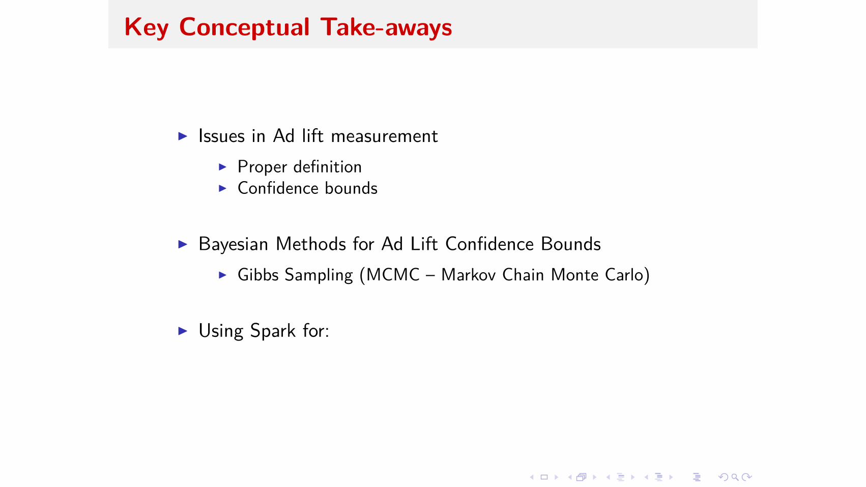
Key Conceptual Take-aways
I Issues in Ad lift measurementI Proper definitionI Confidence bounds
I Bayesian Methods for Ad Lift Confidence BoundsI Gibbs Sampling (MCMC – Markov Chain Monte Carlo)
I Using Spark for:I Monte Carlo sampling for confidence-boundsI Monte Carlo simulations

Application context: ad impact measurement
I Advertisers want to know the impact of showing ads to users.

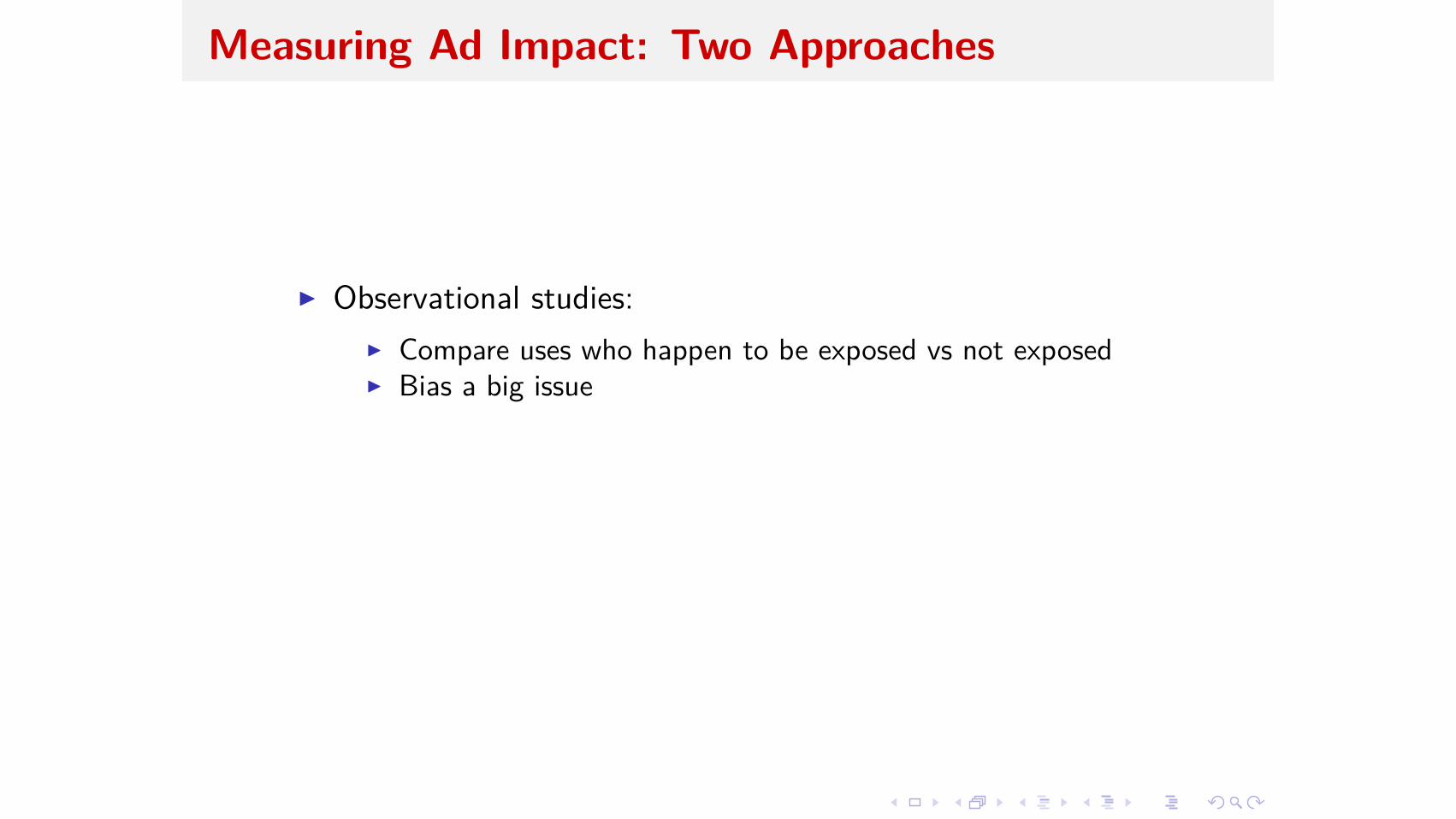
Measuring Ad Impact: Two Approaches
I Observational studies:
I Compare uses who happen to be exposed vs not exposedI Bias a big issue
I Randomized tests:
I Randomly expose to test, compare with control (un-exposed)

Measuring Ad Impact: Two Approaches
I Observational studies:I Compare uses who happen to be exposed vs not exposed
I Bias a big issue
I Randomized tests:
I Randomly expose to test, compare with control (un-exposed)
Measuring Ad Impact: Two Approaches
I Observational studies:I Compare uses who happen to be exposed vs not exposedI Bias a big issue
I Randomized tests:
I Randomly expose to test, compare with control (un-exposed)

Measuring Ad Impact: Two Approaches
I Observational studies:I Compare uses who happen to be exposed vs not exposedI Bias a big issue
I Randomized tests:
I Randomly expose to test, compare with control (un-exposed)

Measuring Ad Impact: Two Approaches
I Observational studies:I Compare uses who happen to be exposed vs not exposedI Bias a big issue
I Randomized tests:I Randomly expose to test, compare with control (un-exposed)

Ideal Randomized Test

Ideal Randomized Test

Ideal Randomized Test

Ideal Randomized Test: Ad lift

Ideal Randomized Test: Ad lift

Ad Lift: Response Rates
If we see k = 200 conversions out of N = 10, 000 users,
what is a good estimate for the response-rate?
Estimated response-rate R̂ = k/N = 200/10, 000 = 2%. . .But how confident are we?

Ad Lift: Response Rates
If we see k = 200 conversions out of N = 10, 000 users,
what is a good estimate for the response-rate?
Estimated response-rate R̂ = k/N = 200/10, 000 = 2%. . .
But how confident are we?

Ad Lift: Response Rates
If we see k = 200 conversions out of N = 10, 000 users,
what is a good estimate for the response-rate?
Estimated response-rate R̂ = k/N = 200/10, 000 = 2%. . .But how confident are we?

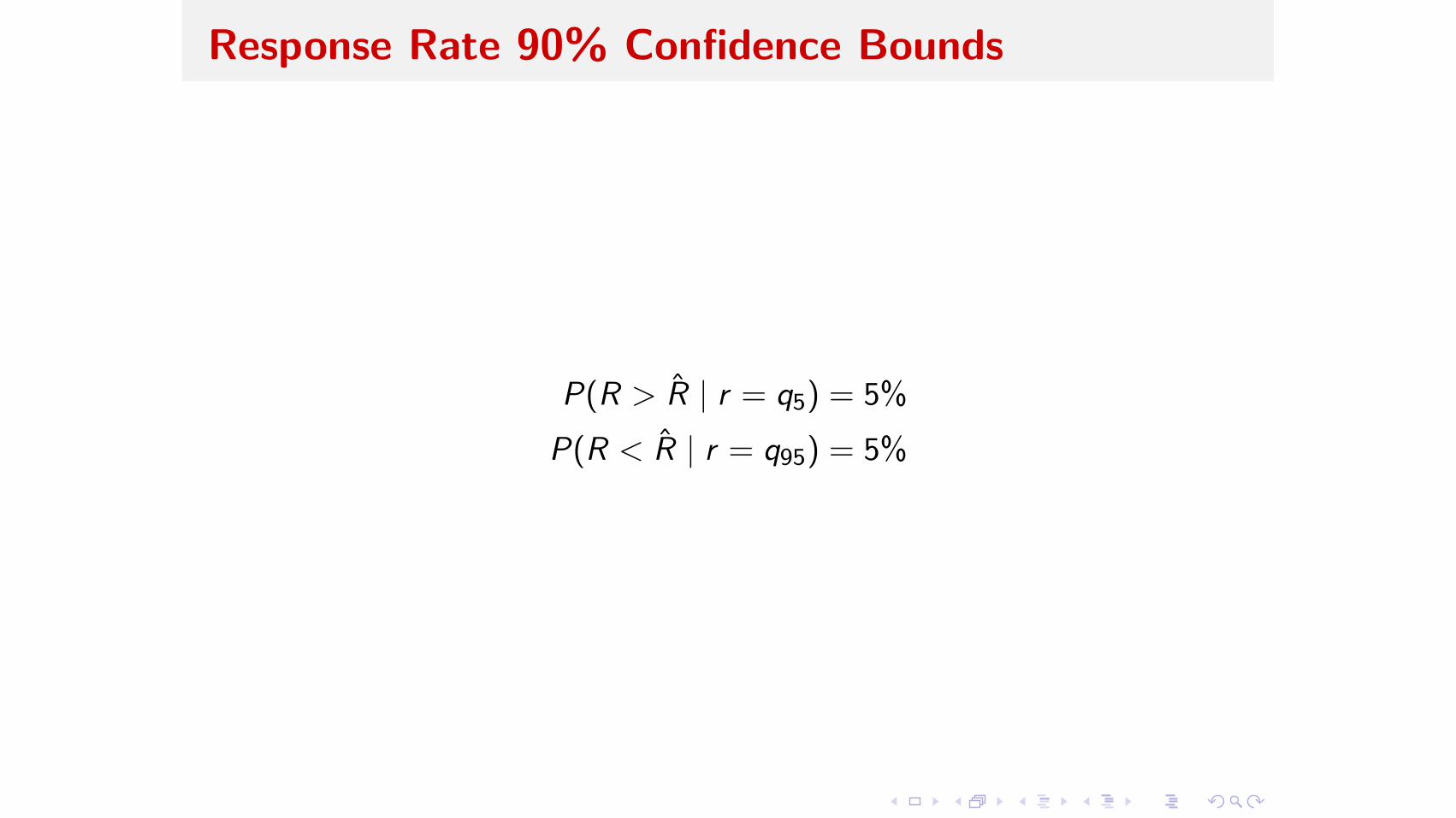
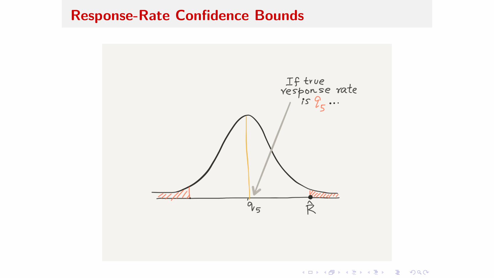
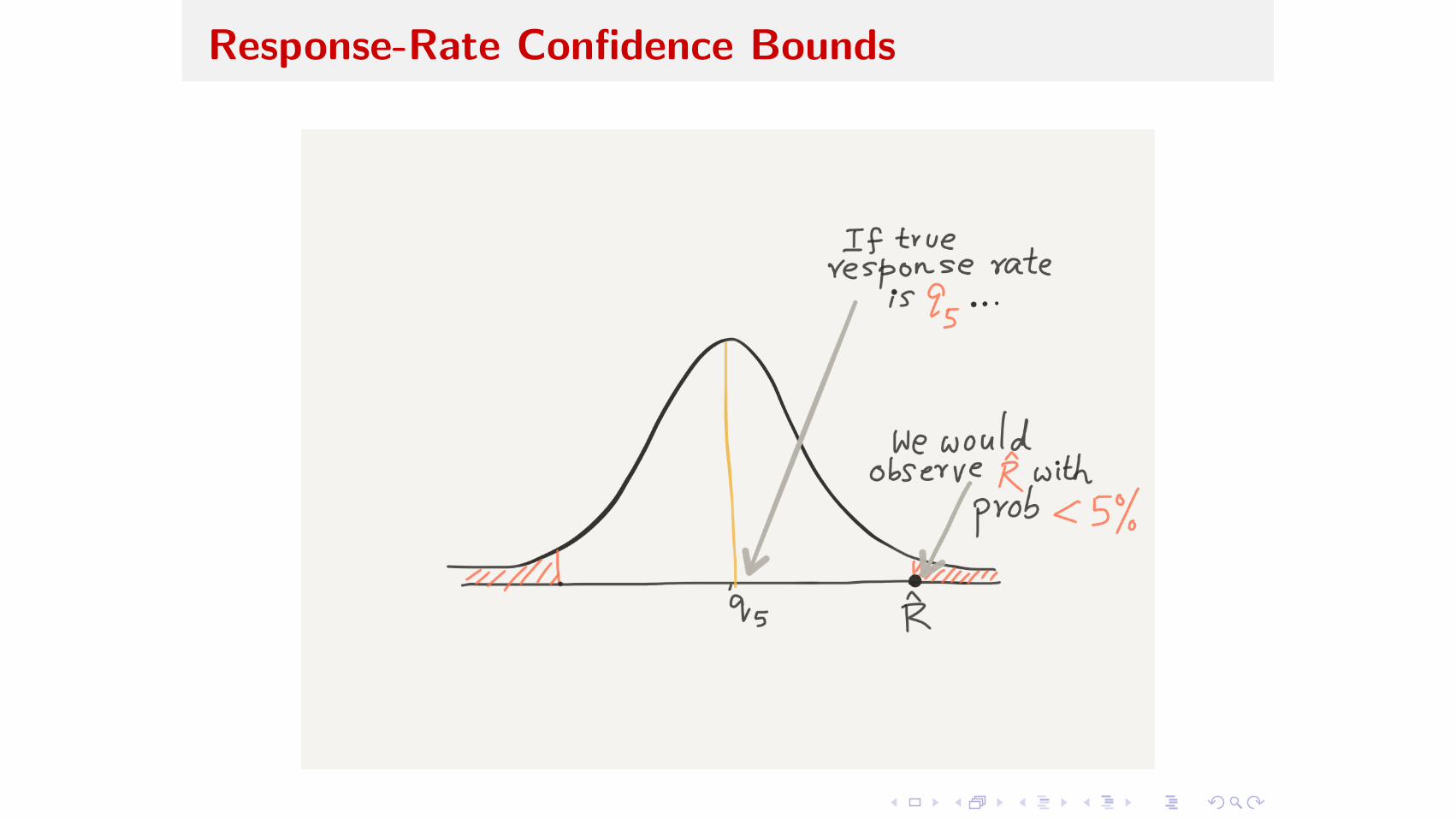
Response Rate 90% Confidence Bounds
P(R > R̂ | r = q5) = 5%P(R < R̂ | r = q95) = 5%

Response Rate 90% Confidence Bounds
P(R > R̂ | r = q5) = 5%
P(R < R̂ | r = q95) = 5%
Response Rate 90% Confidence Bounds
P(R > R̂ | r = q5) = 5%P(R < R̂ | r = q95) = 5%

Response-Rate Confidence Bounds
Response-Rate Confidence Bounds
Response-Rate Confidence Bounds

Response-Rate Confidence Bounds
How to find (q5, q95) ?


Response-Rate: Bayesian Confidence Bounds
Randomly generate response rates that are consistent with the data.
(Sample rates from posterior distribution given data.)Find the (0.05, 0.95) quantiles of these rates.

Response-Rate: Bayesian Confidence Bounds
Randomly generate response rates that are consistent with the data.(Sample rates from posterior distribution given data.)
Find the (0.05, 0.95) quantiles of these rates.

Response-Rate: Bayesian Confidence Bounds
Randomly generate response rates that are consistent with the data.(Sample rates from posterior distribution given data.)Find the (0.05, 0.95) quantiles of these rates.

Response-Rate: Bayesian Confidence Bounds
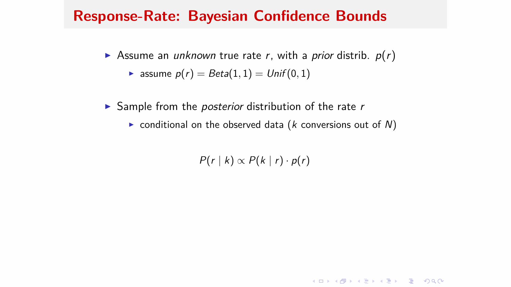
I Assume an unknown true rate r , with a prior distrib. p(r)I assume p(r) = Beta(1, 1) = Unif (0, 1)
I Sample from the posterior distribution of the rate r
I conditional on the observed data (k conversions out of N)
P(r | k) Ã P(k | r) · p(r)
à r
k(1 ≠ r)N≠k · Beta(1, 1)Ã r
k+1(1 ≠ r)N≠k+1
à Beta(k + 1, N ≠ k + 1)
I Compute (0.05, 0.95) quantiles from the generated rates.
Response-Rate: Bayesian Confidence Bounds
I Assume an unknown true rate r , with a prior distrib. p(r)I assume p(r) = Beta(1, 1) = Unif (0, 1)
I Sample from the posterior distribution of the rate r
I conditional on the observed data (k conversions out of N)
P(r | k) Ã P(k | r) · p(r)
à r
k(1 ≠ r)N≠k · Beta(1, 1)Ã r
k+1(1 ≠ r)N≠k+1
à Beta(k + 1, N ≠ k + 1)
I Compute (0.05, 0.95) quantiles from the generated rates.

Response-Rate: Bayesian Confidence Bounds
I Assume an unknown true rate r , with a prior distrib. p(r)I assume p(r) = Beta(1, 1) = Unif (0, 1)
I Sample from the posterior distribution of the rate r
I conditional on the observed data (k conversions out of N)
P(r | k) Ã P(k | r) · p(r)Ã r
k(1 ≠ r)N≠k · Beta(1, 1)
à r
k+1(1 ≠ r)N≠k+1
à Beta(k + 1, N ≠ k + 1)
I Compute (0.05, 0.95) quantiles from the generated rates.

Response-Rate: Bayesian Confidence Bounds
I Assume an unknown true rate r , with a prior distrib. p(r)I assume p(r) = Beta(1, 1) = Unif (0, 1)
I Sample from the posterior distribution of the rate r
I conditional on the observed data (k conversions out of N)
P(r | k) Ã P(k | r) · p(r)Ã r
k(1 ≠ r)N≠k · Beta(1, 1)Ã r
k+1(1 ≠ r)N≠k+1
à Beta(k + 1, N ≠ k + 1)
I Compute (0.05, 0.95) quantiles from the generated rates.

Response-Rate: Bayesian Confidence Bounds
I Assume an unknown true rate r , with a prior distrib. p(r)I assume p(r) = Beta(1, 1) = Unif (0, 1)
I Sample from the posterior distribution of the rate r
I conditional on the observed data (k conversions out of N)
P(r | k) Ã P(k | r) · p(r)Ã r
k(1 ≠ r)N≠k · Beta(1, 1)Ã r
k+1(1 ≠ r)N≠k+1
à Beta(k + 1, N ≠ k + 1)
I Compute (0.05, 0.95) quantiles from the generated rates.

Response-Rate: Bayesian Confidence Bounds
A simple form of Gibbs Sampling (more later):
I sample M values of r from posteriorP(r | k) ≥ Beta(k + 1, N ≠ k + 1).
I compute (0.05, 0.95) quantiles
from numpy.random import beta
from scipy.stats.mstats import mquantiles
def conf(N, k, samples = 500):
rates = beta(k+1, N-k+1, samples)
return mquantiles(rates, prob = [0.05, 0.95])

Response-Rate: Bayesian Confidence Bounds

Response-Rate: Bayesian Confidence Bounds

Response-Rate: Bayesian Confidence Bounds

Response-Rate: Bayesian Confidence Bounds

Response-Rate: Bayesian Confidence Bounds

Response Rates: Example
If we see k = 200 conversions out of N = 10, 000 users,
what is a good estimate for the response-rate?
Estimated response-rate R̂ = k/N = 200/10, 000 = 2%. . .
=∆ 90% confidence region (1.8%, 2.2%)

Response Rates: Example
If we see k = 200 conversions out of N = 10, 000 users,
what is a good estimate for the response-rate?
Estimated response-rate R̂ = k/N = 200/10, 000 = 2%. . .=∆ 90% confidence region (1.8%, 2.2%)

We’ve talked about Response Rates. . .
now let’s consider Ad Lift

Ad Lift: Simple Example
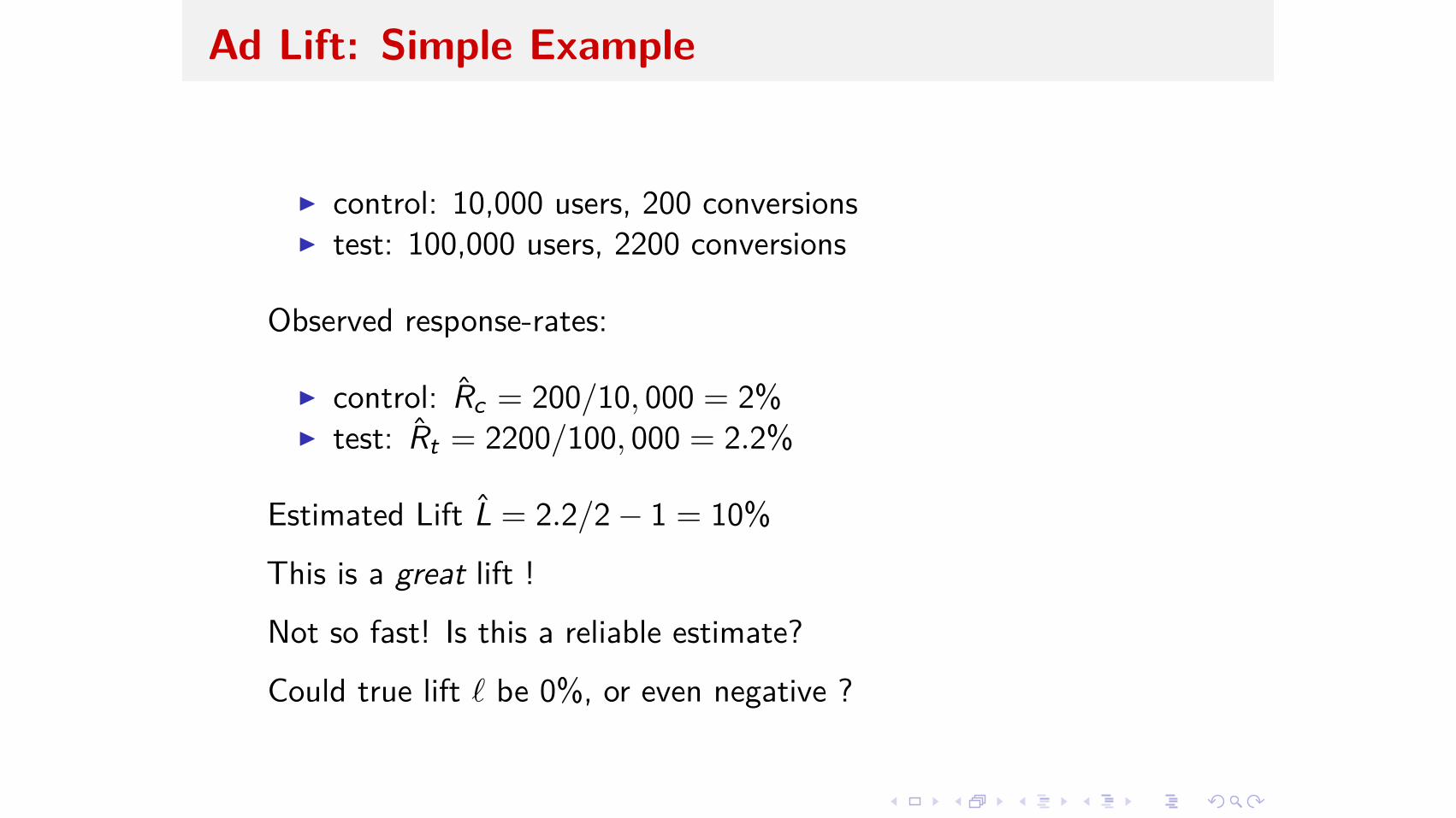
I control: 10,000 users, 200 conversionsI test: 100,000 users, 2200 conversions
Observed response-rates:
I control: R̂c = 200/10, 000 = 2%I test: R̂t = 2200/100, 000 = 2.2%
Estimated Lift L̂ = 2.2/2 ≠ 1 = 10%
This is a great lift !Not so fast! Is this a reliable estimate?Could true lift ¸ be 0%, or even negative ?

Ad Lift: Simple Example
I control: 10,000 users, 200 conversionsI test: 100,000 users, 2200 conversions
Observed response-rates:
I control: R̂c = 200/10, 000 = 2%I test: R̂t = 2200/100, 000 = 2.2%
Estimated Lift L̂ = 2.2/2 ≠ 1 = 10%This is a great lift !
Not so fast! Is this a reliable estimate?Could true lift ¸ be 0%, or even negative ?

Ad Lift: Simple Example
I control: 10,000 users, 200 conversionsI test: 100,000 users, 2200 conversions
Observed response-rates:
I control: R̂c = 200/10, 000 = 2%I test: R̂t = 2200/100, 000 = 2.2%
Estimated Lift L̂ = 2.2/2 ≠ 1 = 10%This is a great lift !Not so fast! Is this a reliable estimate?
Could true lift ¸ be 0%, or even negative ?
Ad Lift: Simple Example
I control: 10,000 users, 200 conversionsI test: 100,000 users, 2200 conversions
Observed response-rates:
I control: R̂c = 200/10, 000 = 2%I test: R̂t = 2200/100, 000 = 2.2%
Estimated Lift L̂ = 2.2/2 ≠ 1 = 10%This is a great lift !Not so fast! Is this a reliable estimate?Could true lift ¸ be 0%, or even negative ?

Ad Lift: Bayesian Confidence Bounds
Sampling approach:Observed data: control: (kc , Nc), test: (kt , Nt)
1. Repeat M times:
I draw control response rate rc from posterior
P(rc | kc) ≥ Beta(kc + 1, Nc ≠ kc + 1).
I draw test response rate rt from posterior
P(rt | kt) ≥ Beta(kt + 1, Nt ≠ kt + 1).
I compute lift L = rt/rc ≠ 1
2. Compute (0.05, 0.95) quantiles of set of M lifts {L}.

Ad Lift: Bayesian Confidence Intervals
I control: nc = 10, 000 users, kc = 200 conversionsI test: nt = 100, 000 users, kt = 2, 200 conversions
Observed response-rates:
I control: R̂c = 200/10, 000 = 2%I test: R̂t = 2200/100, 000 = 2.2%
Estimated Lift L̂ = 2.2/2 ≠ 1 = 10%
90% confidence interval: (≠2.7%, 23.6%)

Ad Lift: Bayesian Confidence Intervals
I control: nc = 10, 000 users, kc = 200 conversionsI test: nt = 100, 000 users, kt = 2, 200 conversions
Observed response-rates:
I control: R̂c = 200/10, 000 = 2%I test: R̂t = 2200/100, 000 = 2.2%
Estimated Lift L̂ = 2.2/2 ≠ 1 = 10%90% confidence interval: (≠2.7%, 23.6%)


Complication 1:
Auction win-bias
Ideal Randomized Test

Ideal Randomized Test

Ideal Randomized Test
Bids on control users are wasted!

Ideal Randomized Test
Bids on control users are wasted!


A Less Wasteful Randomized Test

A Less Wasteful Randomized Test: Win-bias
Cannot simply compare Test Winners (tw) and Control (c):
I test-winners selection bias: “win bias”

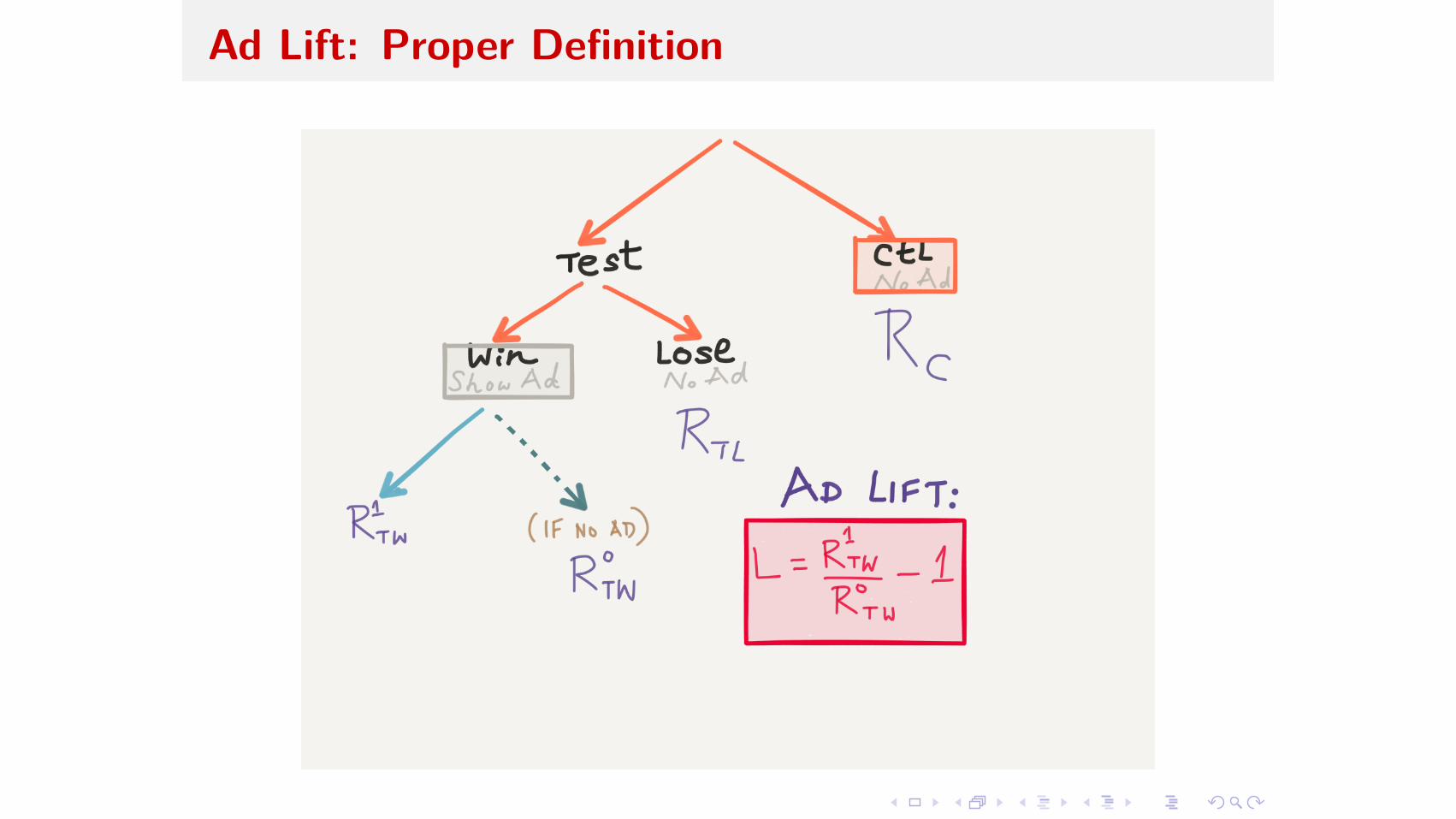
Ad Lift: Proper Definition

Ad Lift: Proper Definition

Ad Lift: Proper Definition

Ad Lift: Proper Definition

Ad Lift: Proper Definition
Ad Lift: Proper Definition
Ad Lift Estimation
Main ideas:
I observe test-losers response rate RtL
I observe test win-rate w
I we show one can estimate
R
0tw = Rc ≠ (1 ≠ w)RtL
w
I compute lift L = R
1tw /R
0tw ≠ 1
I similar to Treatment E�ect Under Non-compliance in clinicialtrials.
Ad Lift Estimation
Main ideas:
I observe test-losers response rate RtL
I observe test win-rate w
I we show one can estimate
R
0tw = Rc ≠ (1 ≠ w)RtL
w
I compute lift L = R
1tw /R
0tw ≠ 1
I similar to Treatment E�ect Under Non-compliance in clinicialtrials.

Ad Lift Estimation
Main ideas:
I observe test-losers response rate RtL
I observe test win-rate w
I we show one can estimate
R
0tw = Rc ≠ (1 ≠ w)RtL
w
I compute lift L = R
1tw /R
0tw ≠ 1
I similar to Treatment E�ect Under Non-compliance in clinicialtrials.

Ad Lift Estimation
Main ideas:
I observe test-losers response rate RtL
I observe test win-rate w
I we show one can estimate
R
0tw = Rc ≠ (1 ≠ w)RtL
w
I compute lift L = R
1tw /R
0tw ≠ 1
I similar to Treatment E�ect Under Non-compliance in clinicialtrials.

Ad Lift Estimation
Main ideas:
I observe test-losers response rate RtL
I observe test win-rate w
I we show one can estimate
R
0tw = Rc ≠ (1 ≠ w)RtL
w
I compute lift L = R
1tw /R
0tw ≠ 1
I similar to Treatment E�ect Under Non-compliance in clinicialtrials.
Ad Lift Estimation
How to compute the 90% confidence interval for L?


Ad Lift: Confidence Intervals with Gibbs sampler
Bayesian approach (details omitted, see Chickering/Pearl 1997):
I Assume a random parameter vector ◊ consisting of:
I user latent (potential) behaviorsI their probabilities
I Set up prior distribution on ◊ ≥ p(◊) (Dirichlet)
I Sample M values of unknown ◊ from posterior: Gibbs Sampler
P(◊ |Data) Ã P(Data | ◊) · p(◊)
I For each sampled ◊ compute lift L using above
I Compute (0.05, 0.95) quantiles of sampled L values

Ad Lift: Confidence Intervals with Gibbs sampler
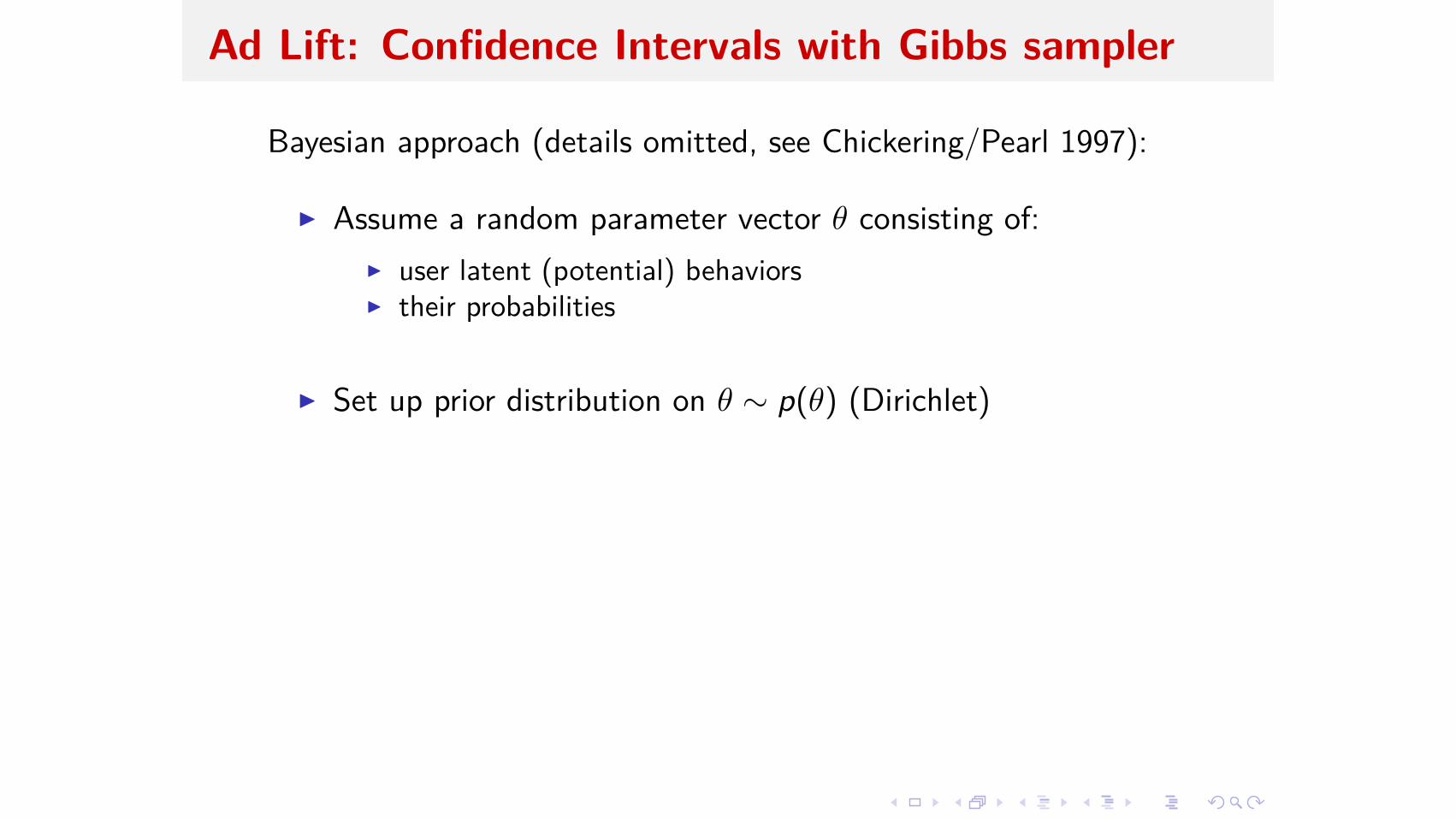
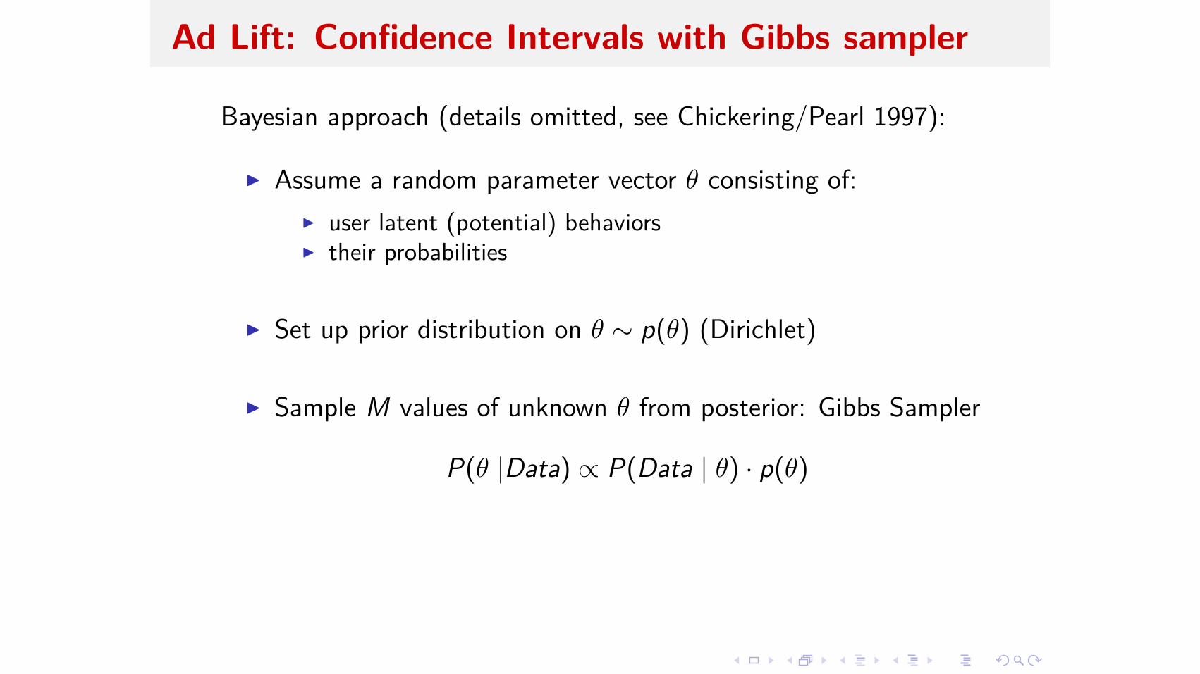
Bayesian approach (details omitted, see Chickering/Pearl 1997):
I Assume a random parameter vector ◊ consisting of:I user latent (potential) behaviors
I their probabilities
I Set up prior distribution on ◊ ≥ p(◊) (Dirichlet)
I Sample M values of unknown ◊ from posterior: Gibbs Sampler
P(◊ |Data) Ã P(Data | ◊) · p(◊)
I For each sampled ◊ compute lift L using above
I Compute (0.05, 0.95) quantiles of sampled L values

Ad Lift: Confidence Intervals with Gibbs sampler
Bayesian approach (details omitted, see Chickering/Pearl 1997):
I Assume a random parameter vector ◊ consisting of:I user latent (potential) behaviorsI their probabilities
I Set up prior distribution on ◊ ≥ p(◊) (Dirichlet)
I Sample M values of unknown ◊ from posterior: Gibbs Sampler
P(◊ |Data) Ã P(Data | ◊) · p(◊)
I For each sampled ◊ compute lift L using above
I Compute (0.05, 0.95) quantiles of sampled L values

Ad Lift: Confidence Intervals
Gibbs sampler convergence may depend on prior distribution:
I start with multiple (say 100) priorsI run them all in parallel using Spark.

Ad Lift: Confidence Intervals
Gibbs sampler convergence may depend on prior distribution:
I start with multiple (say 100) priorsI run them all in parallel using Spark.

Uses of Monte Carlo Simulations
I confidence intervals
I determine “su�cient” population sizes for reliably estimating
I response ratesI lift
I understand e�ect of complex phenomena
I validate/verify analytical formulas
Uses of Monte Carlo Simulations
I confidence intervals
I determine “su�cient” population sizes for reliably estimating
I response ratesI lift
I understand e�ect of complex phenomena
I validate/verify analytical formulas

Uses of Monte Carlo Simulations
I confidence intervals
I determine “su�cient” population sizes for reliably estimatingI response rates
I lift
I understand e�ect of complex phenomena
I validate/verify analytical formulas

Uses of Monte Carlo Simulations
I confidence intervals
I determine “su�cient” population sizes for reliably estimatingI response ratesI lift
I understand e�ect of complex phenomena
I validate/verify analytical formulas

Uses of Monte Carlo Simulations
I confidence intervals
I determine “su�cient” population sizes for reliably estimatingI response ratesI lift
I understand e�ect of complex phenomena
I validate/verify analytical formulas

Uses of Monte Carlo Simulations
I confidence intervals
I determine “su�cient” population sizes for reliably estimatingI response ratesI lift
I understand e�ect of complex phenomenaI validate/verify analytical formulas

Complication 2:
Control contamination due to users with multiple cookies


Control Contamination due to Multiple Cookies

Control Contamination due to Multiple Cookies

Control Contamination due to Multiple Cookies

Control Contamination due to Multiple Cookies

Control Contamination due to Multiple Cookies

Cookie-Contamination Questions
I How does cookie contamination a�ect measured lift?
I Does the cookie-distribution matter?
I everyone has k cookies vs an average of k cookies
I What is the influence of the control percentage?
I Simulations best way to understand this

Cookie-Contamination Questions
I How does cookie contamination a�ect measured lift?
I Does the cookie-distribution matter?
I everyone has k cookies vs an average of k cookies
I What is the influence of the control percentage?
I Simulations best way to understand this

Cookie-Contamination Questions
I How does cookie contamination a�ect measured lift?
I Does the cookie-distribution matter?I everyone has k cookies vs an average of k cookies
I What is the influence of the control percentage?
I Simulations best way to understand this

Cookie-Contamination Questions
I How does cookie contamination a�ect measured lift?
I Does the cookie-distribution matter?I everyone has k cookies vs an average of k cookies
I What is the influence of the control percentage?
I Simulations best way to understand this

Cookie-Contamination Questions
I How does cookie contamination a�ect measured lift?
I Does the cookie-distribution matter?I everyone has k cookies vs an average of k cookies
I What is the influence of the control percentage?
I Simulations best way to understand this

Simulations for cookie-contamination
I A scenario is a combination of parameters:I
M = # trials for this scenario, usually 10K-1MI
n = # users, typically 10K - 10MI
p = # control percentage (usually 10-50%)I
k = cookie-distribution, expressed as 1 : 100, or 1 : 70, 3 : 30I
r = (un-contaminated) control user response rateI
a = true lift, i.e. exposed user response rate = r ú (1 + a).I A scenario file specifies a scenario in each row.
I could be thousands of scenarios

Scenario Simulations in Spark

Scenario Simulations in Spark

Scenario Simulations in Spark

Scenario Simulations in Spark

Scenario Simulations in Spark