Embed Size (px)
Citation preview

An Overview of Graph Data Management and Analysis
M. Tamer Ozsu
University of WaterlooDavid R. Cheriton School of Computer Science
© M. Tamer Ozsu Croucher ASI (2015/12/16-18) 1 / 96

Graph Data are Very Common
Internet
© M. Tamer Ozsu Croucher ASI (2015/12/16-18) 2 / 96

Graph Data are Very Common
Socialnetworks
© M. Tamer Ozsu Croucher ASI (2015/12/16-18) 2 / 96

Graph Data are Very Common
Trade volumesand
connections
© M. Tamer Ozsu Croucher ASI (2015/12/16-18) 2 / 96

Graph Data are Very Common
Biologicalnetworks
© M. Tamer Ozsu Croucher ASI (2015/12/16-18) 2 / 96

Graph Data are Very Common
As of September 2011
MusicBrainz
(zitgist)
P20
Turismo de
Zaragoza
yovisto
Yahoo! Geo
Planet
YAGO
World Fact-book
El ViajeroTourism
WordNet (W3C)
WordNet (VUA)
VIVO UF
VIVO Indiana
VIVO Cornell
VIAF
URIBurner
Sussex Reading
Lists
Plymouth Reading
Lists
UniRef
UniProt
UMBEL
UK Post-codes
legislationdata.gov.uk
Uberblic
UB Mann-heim
TWC LOGD
Twarql
transportdata.gov.
uk
Traffic Scotland
theses.fr
Thesau-rus W
totl.net
Tele-graphis
TCMGeneDIT
TaxonConcept
Open Library (Talis)
tags2con delicious
t4gminfo
Swedish Open
Cultural Heritage
Surge Radio
Sudoc
STW
RAMEAU SH
statisticsdata.gov.
uk
St. Andrews Resource
Lists
ECS South-ampton EPrints
SSW Thesaur
us
SmartLink
Slideshare2RDF
semanticweb.org
SemanticTweet
Semantic XBRL
SWDog Food
Source Code Ecosystem Linked Data
US SEC (rdfabout)
Sears
Scotland Geo-
graphy
ScotlandPupils &Exams
Scholaro-meter
WordNet (RKB
Explorer)
Wiki
UN/LOCODE
Ulm
ECS (RKB
Explorer)
Roma
RISKS
RESEX
RAE2001
Pisa
OS
OAI
NSF
New-castle
LAASKISTI
JISC
IRIT
IEEE
IBM
Eurécom
ERA
ePrints dotAC
DEPLOY
DBLP (RKB
Explorer)
Crime Reports
UK
Course-ware
CORDIS (RKB
Explorer)CiteSeer
Budapest
ACM
riese
Revyu
researchdata.gov.
ukRen. Energy Genera-
tors
referencedata.gov.
uk
Recht-spraak.
nl
RDFohloh
Last.FM (rdfize)
RDF Book
Mashup
Rådata nå!
PSH
Product Types
Ontology
ProductDB
PBAC
Poké-pédia
patentsdata.go
v.uk
OxPoints
Ord-nance Survey
Openly Local
Open Library
OpenCyc
Open Corpo-rates
OpenCalais
OpenEI
Open Election
Data Project
OpenData
Thesau-rus
Ontos News Portal
OGOLOD
JanusAMP
Ocean Drilling Codices
New York
Times
NVD
ntnusc
NTU Resource
Lists
Norwe-gian
MeSH
NDL subjects
ndlna
myExperi-ment
Italian Museums
medu-cator
MARC Codes List
Man-chester Reading
Lists
Lotico
Weather Stations
London Gazette
LOIUS
Linked Open Colors
lobidResources
lobidOrgani-sations
LEM
LinkedMDB
LinkedLCCN
LinkedGeoData
LinkedCT
LinkedUser
FeedbackLOV
Linked Open
Numbers
LODE
Eurostat (OntologyCentral)
Linked EDGAR
(OntologyCentral)
Linked Crunch-
base
lingvoj
Lichfield Spen-ding
LIBRIS
Lexvo
LCSH
DBLP (L3S)
Linked Sensor Data (Kno.e.sis)
Klapp-stuhl-club
Good-win
Family
National Radio-activity
JP
Jamendo (DBtune)
Italian public
schools
ISTAT Immi-gration
iServe
IdRef Sudoc
NSZL Catalog
Hellenic PD
Hellenic FBD
PiedmontAccomo-dations
GovTrack
GovWILD
GoogleArt
wrapper
gnoss
GESIS
GeoWordNet
GeoSpecies
GeoNames
GeoLinkedData
GEMET
GTAA
STITCH
SIDER
Project Guten-berg
MediCare
Euro-stat
(FUB)
EURES
DrugBank
Disea-some
DBLP (FU
Berlin)
DailyMed
CORDIS(FUB)
Freebase
flickr wrappr
Fishes of Texas
Finnish Munici-palities
ChEMBL
FanHubz
EventMedia
EUTC Produc-
tions
Eurostat
Europeana
EUNIS
EU Insti-
tutions
ESD stan-dards
EARTh
Enipedia
Popula-tion (En-AKTing)
NHS(En-
AKTing) Mortality(En-
AKTing)
Energy (En-
AKTing)
Crime(En-
AKTing)
CO2 Emission
(En-AKTing)
EEA
SISVU
education.data.g
ov.uk
ECS South-ampton
ECCO-TCP
GND
Didactalia
DDC Deutsche Bio-
graphie
datadcs
MusicBrainz
(DBTune)
Magna-tune
John Peel
(DBTune)
Classical (DB
Tune)
AudioScrobbler (DBTune)
Last.FM artists
(DBTune)
DBTropes
Portu-guese
DBpedia
dbpedia lite
Greek DBpedia
DBpedia
data-open-ac-uk
SMCJournals
Pokedex
Airports
NASA (Data Incu-bator)
MusicBrainz(Data
Incubator)
Moseley Folk
Metoffice Weather Forecasts
Discogs (Data
Incubator)
Climbing
data.gov.uk intervals
Data Gov.ie
databnf.fr
Cornetto
reegle
Chronic-ling
America
Chem2Bio2RDF
Calames
businessdata.gov.
uk
Bricklink
Brazilian Poli-
ticians
BNB
UniSTS
UniPathway
UniParc
Taxonomy
UniProt(Bio2RDF)
SGD
Reactome
PubMedPub
Chem
PRO-SITE
ProDom
Pfam
PDB
OMIMMGI
KEGG Reaction
KEGG Pathway
KEGG Glycan
KEGG Enzyme
KEGG Drug
KEGG Com-pound
InterPro
HomoloGene
HGNC
Gene Ontology
GeneID
Affy-metrix
bible ontology
BibBase
FTS
BBC Wildlife Finder
BBC Program
mes BBC Music
Alpine Ski
Austria
LOCAH
Amster-dam
Museum
AGROVOC
AEMET
US Census (rdfabout)
Media
Geographic
Publications
Government
Cross-domain
Life sciences
User-generated content
Linked data
© M. Tamer Ozsu Croucher ASI (2015/12/16-18) 2 / 96
Linking Open Data cloud diagram, by Richard Cyganiak and Anja Jentzsch.http://lod-cloud.net/

Outline
1 Introduction – Graph Types
2 Property Graph ProcessingClassificationOnline queryingOffline analytics
3 RDF Graph QueryingData WarehousingDistributed SPARQL ExecutionLinked Object Data Querying
© M. Tamer Ozsu Croucher ASI (2015/12/16-18) 3 / 96

Outline
1 Introduction – Graph Types
2 Property Graph ProcessingClassificationOnline queryingOffline analytics
3 RDF Graph QueryingData WarehousingDistributed SPARQL ExecutionLinked Object Data Querying
© M. Tamer Ozsu Croucher ASI (2015/12/16-18) 4 / 96
Graph Types
Property graph
film 2014(initial release date, “1980-05-23”)
(label, “The Shining”)
books 0743424425(rating, 4.7)
offers 0743424425amazonOffer
geo 2635167(name, “United Kingdom”)
(population, 62348447) actor 29704(actor name, “Jack Nicholson”)
film 3418(label, “The Passenger”)
film 1267(label, “The Last Tycoon”)
director 8476(director name, “Stanley Kubrick”)
film 2685(label, “A Clockwork Orange”)
film 424(label, “Spartacus”)
actor 30013
(relatedBook)
(hasOffer)
(based near)(actor)
(director) (actor)
(actor) (actor)
(director) (director)
© M. Tamer Ozsu Croucher ASI (2015/12/16-18) 5 / 96

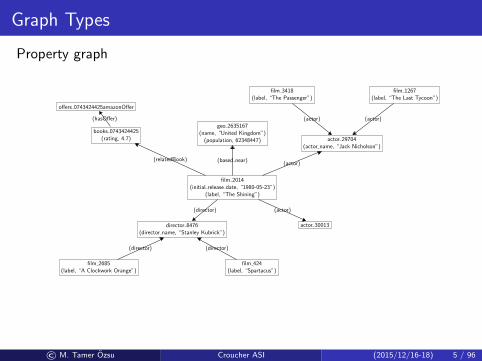
Graph Types
RDF graph
mdb:film/2014
“1980-05-23”
movie:initial release date
“The Shining”refs:label
bm:books/0743424425
4.7
rev:rating
bm:offers/0743424425amazonOffer
geo:2635167
“United Kingdom”
gn:name
62348447
gn:population
mdb:actor/29704
“Jack Nicholson”
movie:actor name
mdb:film/3418
“The Passenger”
refs:label
mdb:film/1267
“The Last Tycoon”
refs:label
mdb:director/8476
“Stanley Kubrick”
movie:director name
mdb:film/2685
“A Clockwork Orange”
refs:label
mdb:film/424
“Spartacus”
refs:label
mdb:actor/30013
movie:relatedBook
scam:hasOffer
foaf:based nearmovie:actor
movie:directormovie:actor
movie:actor movie:actor
movie:director movie:director
© M. Tamer Ozsu Croucher ASI (2015/12/16-18) 5 / 96

Graph Types
Property graph
film 2014(initial release date, “1980-05-23”)
(label, “The Shining”)
books 0743424425(rating, 4.7)
offers 0743424425amazonOffer
geo 2635167(name, “United Kingdom”)
(population, 62348447) actor 29704(actor name, “Jack Nicholson”)
film 3418(label, “The Passenger”)
film 1267(label, “The Last Tycoon”)
director 8476(director name, “Stanley Kubrick”)
film 2685(label, “A Clockwork Orange”)
film 424(label, “Spartacus”)
actor 30013
(relatedBook)
(hasOffer)
(based near)(actor)
(director) (actor)
(actor) (actor)
(director) (director)
Workload: Online queries andanalytic workloads
Query execution: Varies
RDF graph
mdb:film/2014
“1980-05-23”
movie:initial release date
“The Shining”refs:label
bm:books/0743424425
4.7
rev:rating
bm:offers/0743424425amazonOffer
geo:2635167
“United Kingdom”
gn:name
62348447
gn:population
mdb:actor/29704
“Jack Nicholson”
movie:actor name
mdb:film/3418
“The Passenger”
refs:label
mdb:film/1267
“The Last Tycoon”
refs:label
mdb:director/8476
“Stanley Kubrick”
movie:director name
mdb:film/2685
“A Clockwork Orange”
refs:label
mdb:film/424
“Spartacus”
refs:label
mdb:actor/30013
movie:relatedBook
scam:hasOffer
foaf:based nearmovie:actor
movie:directormovie:actor
movie:actor movie:actor
movie:director movie:director
Workload: SPARQL queries
Query execution: subgraphmatching by homomorphism
© M. Tamer Ozsu Croucher ASI (2015/12/16-18) 5 / 96

Outline
1 Introduction – Graph Types
2 Property Graph ProcessingClassificationOnline queryingOffline analytics
3 RDF Graph QueryingData WarehousingDistributed SPARQL ExecutionLinked Object Data Querying
© M. Tamer Ozsu Croucher ASI (2015/12/16-18) 6 / 96

Outline
1 Introduction – Graph Types
2 Property Graph ProcessingClassificationOnline queryingOffline analytics
3 RDF Graph QueryingData WarehousingDistributed SPARQL ExecutionLinked Object Data Querying
© M. Tamer Ozsu Croucher ASI (2015/12/16-18) 7 / 96

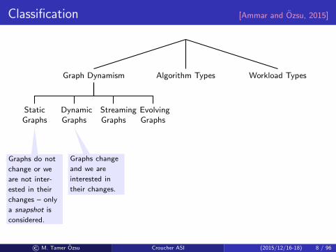
Classification [Ammar and Ozsu, 2015]
Graph Dynamism
StaticGraphs
DynamicGraphs
StreamingGraphs
EvolvingGraphs
Algorithm Types
Offline Online
Streaming Incremental
Dynamic
BatchDynamic
Workload Types
OnlineQueries
AnalyticsWorkloads
© M. Tamer Ozsu Croucher ASI (2015/12/16-18) 8 / 96

Classification [Ammar and Ozsu, 2015]
Graph Dynamism
StaticGraphs
DynamicGraphs
StreamingGraphs
EvolvingGraphs
Algorithm Types
Offline Online
Streaming Incremental
Dynamic
BatchDynamic
Workload Types
OnlineQueries
AnalyticsWorkloads
Focus here is on the
dynamism of the
graphs in whether or
not they change and
how they change.
Focus here is on the
how algorithms behave
as their input changes.
The types of workloads
that the approaches are
designed to handle.
© M. Tamer Ozsu Croucher ASI (2015/12/16-18) 8 / 96

Classification [Ammar and Ozsu, 2015]
Graph Dynamism
StaticGraphs
DynamicGraphs
StreamingGraphs
EvolvingGraphs
Algorithm Types
Offline Online
Streaming Incremental
Dynamic
BatchDynamic
Workload Types
OnlineQueries
AnalyticsWorkloads
© M. Tamer Ozsu Croucher ASI (2015/12/16-18) 8 / 96

Classification [Ammar and Ozsu, 2015]
Graph Dynamism
StaticGraphs
DynamicGraphs
StreamingGraphs
EvolvingGraphs
Algorithm Types
Offline Online
Streaming Incremental
Dynamic
BatchDynamic
Workload Types
OnlineQueries
AnalyticsWorkloads
Graphs do not
change or we
are not inter-
ested in their
changes – only
a snapshot is
considered.
© M. Tamer Ozsu Croucher ASI (2015/12/16-18) 8 / 96
Classification [Ammar and Ozsu, 2015]
Graph Dynamism
StaticGraphs
DynamicGraphs
StreamingGraphs
EvolvingGraphs
Algorithm Types
Offline Online
Streaming Incremental
Dynamic
BatchDynamic
Workload Types
OnlineQueries
AnalyticsWorkloads
Graphs do not
change or we
are not inter-
ested in their
changes – only
a snapshot is
considered.
Graphs change
and we are
interested in
their changes.
© M. Tamer Ozsu Croucher ASI (2015/12/16-18) 8 / 96

Classification [Ammar and Ozsu, 2015]
Graph Dynamism
StaticGraphs
DynamicGraphs
StreamingGraphs
EvolvingGraphs
Algorithm Types
Offline Online
Streaming Incremental
Dynamic
BatchDynamic
Workload Types
OnlineQueries
AnalyticsWorkloads
Graphs do not
change or we
are not inter-
ested in their
changes – only
a snapshot is
considered.
Graphs change
and we are
interested in
their changes.
Dynamic
graphs with
high veloc-
ity changes –
not possible to
see the entire
graph at once.
Dynamic
graphs with un-
known changes
– requires re-
discovery of
the graph (e.g.,
LOD).
© M. Tamer Ozsu Croucher ASI (2015/12/16-18) 8 / 96

Classification [Ammar and Ozsu, 2015]
Graph Dynamism
StaticGraphs
DynamicGraphs
StreamingGraphs
EvolvingGraphs
Algorithm Types
Offline Online
Streaming Incremental
Dynamic
BatchDynamic
Workload Types
OnlineQueries
AnalyticsWorkloads
© M. Tamer Ozsu Croucher ASI (2015/12/16-18) 8 / 96

Classification [Ammar and Ozsu, 2015]
Graph Dynamism
StaticGraphs
DynamicGraphs
StreamingGraphs
EvolvingGraphs
Algorithm Types
Offline Online
Streaming Incremental
Dynamic
BatchDynamic
Workload Types
OnlineQueries
AnalyticsWorkloads
Computation accesses a
portion of the graph
and the results are
computed for a subset
of vertices; e.g., point-
to-point shortest path,
subgraph matching,
reachability, SPARQL.
Computation accesses
the entire graph and
may require multiple
iterations; e.g., PageR-
ank, clustering, graph
colouring, all pairs
shortest path.
© M. Tamer Ozsu Croucher ASI (2015/12/16-18) 8 / 96

Classification [Ammar and Ozsu, 2015]
Graph Dynamism
StaticGraphs
DynamicGraphs
StreamingGraphs
EvolvingGraphs
Algorithm Types
Offline Online
Streaming Incremental
Dynamic
BatchDynamic
Workload Types
OnlineQueries
AnalyticsWorkloads
© M. Tamer Ozsu Croucher ASI (2015/12/16-18) 8 / 96

Classification [Ammar and Ozsu, 2015]
Graph Dynamism
StaticGraphs
DynamicGraphs
StreamingGraphs
EvolvingGraphs
Algorithm Types
Offline Online
Streaming Incremental
Dynamic
BatchDynamic
Workload Types
OnlineQueries
AnalyticsWorkloads
Sees the en-
tire input in
advance.
Sees the input
piece-meal as it
executes.
One-pass on-
line algorithm
with limited
memory.
Online algo-
rithm with
some info
about forth-
coming input.© M. Tamer Ozsu Croucher ASI (2015/12/16-18) 8 / 96

Classification [Ammar and Ozsu, 2015]
Graph Dynamism
StaticGraphs
DynamicGraphs
StreamingGraphs
EvolvingGraphs
Algorithm Types
Offline Online
Streaming Incremental
Dynamic
BatchDynamic
Workload Types
OnlineQueries
AnalyticsWorkloads
Sees the en-
tire input in
advance.
Sees the input
piece-meal as it
executes.
One-pass on-
line algorithm
with limited
memory.
Online algo-
rithm with
some info
about forth-
coming input.
Sees the en-
tire input
in advance,
which may
change; an-
swers computed
as change oc-
curs.
© M. Tamer Ozsu Croucher ASI (2015/12/16-18) 8 / 96

Classification [Ammar and Ozsu, 2015]
Graph Dynamism
StaticGraphs
DynamicGraphs
StreamingGraphs
EvolvingGraphs
Algorithm Types
Offline Online
Streaming Incremental
Dynamic
BatchDynamic
Workload Types
OnlineQueries
AnalyticsWorkloads
Sees the en-
tire input in
advance.
Sees the input
piece-meal as it
executes.
One-pass on-
line algorithm
with limited
memory.
Online algo-
rithm with
some info
about forth-
coming input.
Sees the en-
tire input
in advance,
which may
change; an-
swers computed
as change oc-
curs.
Similar to dy-
namic, but
computation
happens in
batches of
changes.© M. Tamer Ozsu Croucher ASI (2015/12/16-18) 8 / 96

Example Design Points
Graph Dynamism
StaticGraphs
DynamicGraphs
StreamingGraphs
EvolvingGraphs
Algorithm Types
Offline Online
Streaming Incremental
Dynamic
BatchDynamic
Workload Types
OnlineQueries
AnalyticsWorkloads
Compute the query result/perform analytic computation over the graphas it exists.
© M. Tamer Ozsu Croucher ASI (2015/12/16-18) 9 / 96

Example Design Points
Graph Dynamism
StaticGraphs
DynamicGraphs
StreamingGraphs
EvolvingGraphs
Algorithm Types
Offline Online
Streaming Incremental
Dynamic
BatchDynamic
Workload Types
OnlineQueries
AnalyticsWorkloads
Compute the query result/perform analytic computation over the graphas it is revealed.
© M. Tamer Ozsu Croucher ASI (2015/12/16-18) 9 / 96

Example Design Points
Graph Dynamism
StaticGraphs
DynamicGraphs
StreamingGraphs
EvolvingGraphs
Algorithm Types
Offline Online
Streaming Incremental
Dynamic
BatchDynamic
Workload Types
OnlineQueries
AnalyticsWorkloads
Compute the query result/perform analytic computation on each snap-shot from scratch.
© M. Tamer Ozsu Croucher ASI (2015/12/16-18) 9 / 96

Example Design Points
Graph Dynamism
StaticGraphs
DynamicGraphs
StreamingGraphs
EvolvingGraphs
Algorithm Types
Offline Online
Streaming Incremental
Dynamic
BatchDynamic
Workload Types
OnlineQueries
AnalyticsWorkloads
Continuously compute the query result/perform analytic computation asthe input changes.
© M. Tamer Ozsu Croucher ASI (2015/12/16-18) 9 / 96

Example Design Points
Graph Dynamism
StaticGraphs
DynamicGraphs
StreamingGraphs
EvolvingGraphs
Algorithm Types
Offline Online
Streaming Incremental
Dynamic
BatchDynamic
Workload Types
OnlineQueries
AnalyticsWorkloads
Compute the query result/perform analytic computation after a batch ofinput changes.
© M. Tamer Ozsu Croucher ASI (2015/12/16-18) 9 / 96

Example Design Points – Not all alternatives make sense
Graph Dynamism
StaticGraphs
DynamicGraphs
StreamingGraphs
EvolvingGraphs
Algorithm Types
Offline Online
Streaming Incremental
Dynamic
BatchDynamic
Workload Types
OnlineQueries
AnalyticsWorkloads
Dynamic (or batch-dynamic) algorithms do not make sense for staticgraphs.
© M. Tamer Ozsu Croucher ASI (2015/12/16-18) 10 / 96

Graph Processing Systems
System Memory/Disk
ArchitectureComputingparadigm
SupportedWorkloads
Hadoop Disk Parallel/Distributed MapReduce Analytical
Haloop Disk Parallel/Distributed MapReduce Analytical
Pegasus Disk Parallel/Distributed MapReduce Analytical
GraphX Disk Parallel/DistributedMapReduce
(Spark)Analytical
Pregel/Giraph Memory Parallel/Distributed Vertex-Centric Analytical
GraphLab Memory Parallel/Distributed Vertex-Centric Analytical
GraphChi Disk Single machine Vertex-Centric Analytical
Stream Disk Single machine Edge-Centric Analytical
Trinity Memory Parallel/DistributedFlexible using K-V
store on DSMOnline &Analytical
Titan Disk Parallel/DistributedK-V store
(Cassandra)Online
Neo4J Disk Single machineProcedural/Linked-list
Online
© M. Tamer Ozsu Croucher ASI (2015/12/16-18) 11 / 96

Graph Workloads
Online graph querying
Reachability
Single source shortest-path
Subgraph matching
SPARQL queries
Offline graph analytics
PageRank
Clustering
Strongly connectedcomponents
Diameter finding
Graph colouring
All pairs shortest path
Graph pattern mining
Machine learning algorithms(Belief propagation, Gaussiannon-negative matrixfactorization)
© M. Tamer Ozsu Croucher ASI (2015/12/16-18) 12 / 96

Outline
1 Introduction – Graph Types
2 Property Graph ProcessingClassificationOnline queryingOffline analytics
3 RDF Graph QueryingData WarehousingDistributed SPARQL ExecutionLinked Object Data Querying
© M. Tamer Ozsu Croucher ASI (2015/12/16-18) 13 / 96

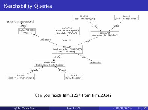
Reachability Queries
film 2014(initial release date, “1980-05-23”)
(label, “The Shining”)
books 0743424425(rating, 4.7)
offers 0743424425amazonOffer
geo 2635167(name, “United Kingdom”)
(population, 62348447) actor 29704(actor name, “Jack Nicholson”)
film 3418(label, “The Passenger”)
film 1267(label, “The Last Tycoon”)
director 8476(director name, “Stanley Kubrick”)
film 2685(label, “A Clockwork Orange”)
film 424(label, “Spartacus”)
actor 30013
(relatedBook)
(hasOffer)
(based near)(actor)
(director) (actor)
(actor) (actor)
(director) (director)
© M. Tamer Ozsu Croucher ASI (2015/12/16-18) 14 / 96
Reachability Queries
film 2014(initial release date, “1980-05-23”)
(label, “The Shining”)
books 0743424425(rating, 4.7)
offers 0743424425amazonOffer
geo 2635167(name, “United Kingdom”)
(population, 62348447) actor 29704(actor name, “Jack Nicholson”)
film 3418(label, “The Passenger”)
film 1267(label, “The Last Tycoon”)
director 8476(director name, “Stanley Kubrick”)
film 2685(label, “A Clockwork Orange”)
film 424(label, “Spartacus”)
actor 30013
(relatedBook)
(hasOffer)
(based near)(actor)
(director) (actor)
(actor) (actor)
(director) (director)
Can you reach film 1267 from film 2014?
© M. Tamer Ozsu Croucher ASI (2015/12/16-18) 14 / 96

Reachability Queries
film 2014(initial release date, “1980-05-23”)
(label, “The Shining”)
books 0743424425(rating, 4.7)
offers 0743424425amazonOffer
geo 2635167(name, “United Kingdom”)
(population, 62348447) actor 29704(actor name, “Jack Nicholson”)
film 3418(label, “The Passenger”)
film 1267(label, “The Last Tycoon”)
director 8476(director name, “Stanley Kubrick”)
film 2685(label, “A Clockwork Orange”)
film 424(label, “Spartacus”)
actor 30013
(relatedBook)
(hasOffer)
(based near)(actor)
(director) (actor)
(actor) (actor)
(director) (director)
Is there a book whose rating is > 4.0 associated with a film that wasdirected by Stanley Kubrick?
© M. Tamer Ozsu Croucher ASI (2015/12/16-18) 14 / 96

Reachability Queries
Think of Facebook graph and finding friends of friends.
© M. Tamer Ozsu Croucher ASI (2015/12/16-18) 14 / 96

Subgraph Matching
?m ?dmovie:director
?name
rdfs:label
?b
movie:relatedBook
“Stanley Kubrick”
movie:director name
?rrev:rating
FILTER(?r > 4.0)
mdb:film/2014
“1980-05-23”
movie:initial release date
“The Shining”refs:label
bm:books/0743424425
4.7
rev:rating
bm:offers/0743424425amazonOffer
geo:2635167
“United Kingdom”
gn:name
62348447
gn:population
mdb:actor/29704
“Jack Nicholson”
movie:actor name
mdb:film/3418
“The Passenger”
refs:label
mdb:film/1267
“The Last Tycoon”
refs:label
mdb:director/8476
“Stanley Kubrick”
movie:director name
mdb:film/2685
“A Clockwork Orange”
refs:label
mdb:film/424
“Spartacus”
refs:label
mdb:actor/30013
movie:relatedBook
scam:hasOffer
foaf:based nearmovie:actor
movie:directormovie:actor
movie:actor movie:actor
movie:director movie:director
SubgraphM
atching
© M. Tamer Ozsu Croucher ASI (2015/12/16-18) 15 / 96

Outline
1 Introduction – Graph Types
2 Property Graph ProcessingClassificationOnline queryingOffline analytics
3 RDF Graph QueryingData WarehousingDistributed SPARQL ExecutionLinked Object Data Querying
© M. Tamer Ozsu Croucher ASI (2015/12/16-18) 16 / 96

PageRank Computation
A web page is important if it is pointed to by other importantpages.
P1 P2
P3
P5P6
P4
r(Pi ) =∑
Pj∈BPi
r(Pj)
|FPj|
r(P2) =r(P1)
2+
r(P3)
3
rk+1(Pi ) =∑
Pj∈BPi
rk(Pj)
|FPj|
BPi: in-neighbours of Pi
FPi: out-neighbours of Pi
© M. Tamer Ozsu Croucher ASI (2015/12/16-18) 17 / 96

PageRank Computation
A web page is important if it is pointed to by other importantpages.
P1 P2
P3
P5P6
P4
rk+1(Pi ) =∑
Pj∈BPi
rk(Pj)
|FPj|
Iteration 0 Iteration 1 Iteration 2Rank atIter. 2
r0(P1) = 1/6 r1(P1) = 1/18 r2(P1) = 1/36 5r0(P2) = 1/6 r1(P2) = 5/36 r2(P2) = 1/18 4r0(P3) = 1/6 r1(P3) = 1/12 r2(P3) = 1/36 5r0(P4) = 1/6 r1(P4) = 1/4 r2(P4) = 17/72 1r0(P5) = 1/6 r1(P5) = 5/36 r2(P5) = 11/72 3r0(P6) = 1/6 r1(P6) = 1/6 r2(P6) = 14/72 2
Iterative processing.
© M. Tamer Ozsu Croucher ASI (2015/12/16-18) 17 / 96

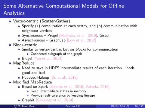
Some Alternative Computational Models for OfflineAnalytics
Vertex-centric (Scatter-Gather)Specify (a) computation at each vertex, and (b) communication withneighbour verticesSynchronous – Pregel [Malewicz et al., 2010], GiraphAsynchronous – GraphLab [Low et al., 2012]
Block-centricSimilar to vertex-centric but on blocks for communication
Connected subgraph of the graph
Blogel [Yan et al., 2014]MapReduce
Need to save in HDFS intermediate results of each iteration – bothgood and badHadoop, Haloop [Bu et al., 2012]
Modified MapReduceBased on Spark [Zaharia et al., 2010; Zaharia, 2016]
Keep intermediate states in memoryProvide fault-tolerance by keeping lineage
GraphX [Gonzalez et al., 2014]
© M. Tamer Ozsu Croucher ASI (2015/12/16-18) 18 / 96

Some Alternative Computational Models for OfflineAnalytics
Vertex-centric (Scatter-Gather)Specify (a) computation at each vertex, and (b) communication withneighbour verticesSynchronous – Pregel [Malewicz et al., 2010], GiraphAsynchronous – GraphLab [Low et al., 2012]
Block-centricSimilar to vertex-centric but on blocks for communication
Connected subgraph of the graph
Blogel [Yan et al., 2014]
MapReduceNeed to save in HDFS intermediate results of each iteration – bothgood and badHadoop, Haloop [Bu et al., 2012]
Modified MapReduceBased on Spark [Zaharia et al., 2010; Zaharia, 2016]
Keep intermediate states in memoryProvide fault-tolerance by keeping lineage
GraphX [Gonzalez et al., 2014]
© M. Tamer Ozsu Croucher ASI (2015/12/16-18) 18 / 96

Some Alternative Computational Models for OfflineAnalytics
Vertex-centric (Scatter-Gather)Specify (a) computation at each vertex, and (b) communication withneighbour verticesSynchronous – Pregel [Malewicz et al., 2010], GiraphAsynchronous – GraphLab [Low et al., 2012]
Block-centricSimilar to vertex-centric but on blocks for communication
Connected subgraph of the graph
Blogel [Yan et al., 2014]MapReduce
Need to save in HDFS intermediate results of each iteration – bothgood and badHadoop, Haloop [Bu et al., 2012]
Modified MapReduceBased on Spark [Zaharia et al., 2010; Zaharia, 2016]
Keep intermediate states in memoryProvide fault-tolerance by keeping lineage
GraphX [Gonzalez et al., 2014]
© M. Tamer Ozsu Croucher ASI (2015/12/16-18) 18 / 96
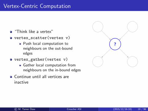
Vertex-Centric Computation
“Think like a vertex”
vertex_scatter(vertex v)
Push local computation toneighbours on the out-boundedges
vertex_gather(vertex v)
Gather local computation fromneighbours on the in-bound edges
Continue until all vertices areinactive
Vertex state machine
?
Active Inactive
Vote halt
Message received
© M. Tamer Ozsu Croucher ASI (2015/12/16-18) 19 / 96

Synchronous Vertex-Centric Computation
Machine 1
Machine 2
Machine 3
Machine 1
Machine 2
Machine 3
Machine 1
Machine 2
Machine 3
CommunicationBarrier
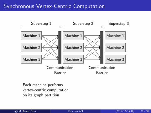
Each machine performsvertex-centric computationon its graph partition
CommunicationBarrier
Superstep 1 Superstep 2 Superstep 3
Computation
© M. Tamer Ozsu Croucher ASI (2015/12/16-18) 20 / 96

Synchronous Vertex-Centric Computation
Machine 1
Machine 2
Machine 3
Machine 1
Machine 2
Machine 3
Machine 1
Machine 2
Machine 3
CommunicationBarrier
Each machine performsvertex-centric computationon its graph partition
CommunicationBarrier
Superstep 1 Superstep 2 Superstep 3
Computation
© M. Tamer Ozsu Croucher ASI (2015/12/16-18) 20 / 96
Asynchronous Vertex-Centric Computation
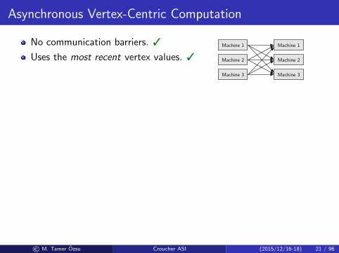
No communication barriers. 3
Uses the most recent vertex values. 3
Implemented via distributed locking
Machine 1
Machine 2
Machine 3
Machine 1
Machine 2
Machine 3
v0
v1 v2
v3 v4
© M. Tamer Ozsu Croucher ASI (2015/12/16-18) 21 / 96

Asynchronous Vertex-Centric Computation
No communication barriers. 3
Uses the most recent vertex values. 3
Implemented via distributed locking
Machine 1
Machine 2
Machine 3
Machine 1
Machine 2
Machine 3
v0
v1 v2
v3 v4
© M. Tamer Ozsu Croucher ASI (2015/12/16-18) 21 / 96

Asynchronous Vertex-Centric Computation
No communication barriers. 3
Uses the most recent vertex values. 3
Implemented via distributed locking
Machine 1
Machine 2
Machine 3
Machine 1
Machine 2
Machine 3
v0
v1 v2
v3 v4
© M. Tamer Ozsu Croucher ASI (2015/12/16-18) 21 / 96

Asynchronous Vertex-Centric Computation
No communication barriers. 3
Uses the most recent vertex values. 3
Implemented via distributed locking
Machine 1
Machine 2
Machine 3
Machine 1
Machine 2
Machine 3
v0
v1 v2
v3 v4
© M. Tamer Ozsu Croucher ASI (2015/12/16-18) 21 / 96

Asynchronous Vertex-Centric Computation
No communication barriers. 3
Uses the most recent vertex values. 3
Implemented via distributed locking
Machine 1
Machine 2
Machine 3
Machine 1
Machine 2
Machine 3
v0
v1 v2
v3 v4
© M. Tamer Ozsu Croucher ASI (2015/12/16-18) 21 / 96

Asynchronous Vertex-Centric Computation
No communication barriers. 3
Uses the most recent vertex values. 3
Implemented via distributed locking
Machine 1
Machine 2
Machine 3
Machine 1
Machine 2
Machine 3
v0
v1 v2
v3 v4
© M. Tamer Ozsu Croucher ASI (2015/12/16-18) 21 / 96

Summary of an Experiment [Han et al., 2014]
A large study comparing Giraph, GraphLab, GPS, Mizan.
1 Giraph scales better across graphs;GraphLab scales better across more machines.
2 Distributed locking for asynchronous execution is not scalable –Performance degrades as more machines are used due to lockcontention, termination scheme, lack of message batching
3 Graph storage should be memory and mutation efficient.
4 Message processing optimizations are very important.
5 Workloads have different resource demands
© M. Tamer Ozsu Croucher ASI (2015/12/16-18) 22 / 96

Summary of an Experiment [Han et al., 2014]
A large study comparing Giraph, GraphLab, GPS, Mizan.
1 Giraph scales better across graphs;GraphLab scales better across more machines.
2 Distributed locking for asynchronous execution is not scalable –Performance degrades as more machines are used due to lockcontention, termination scheme, lack of message batching
3 Graph storage should be memory and mutation efficient.
4 Message processing optimizations are very important.
5 Workloads have different resource demands
64 machines TW UK
Giraph (byte array) 5.8GB 7.0GBGraphLab (sync) 4.5GB 14GB
TW 16 machines 128 machines
Giraph (byte array) 8.5GB 5.8GBGraphLab (sync) 11GB 3.3GB
© M. Tamer Ozsu Croucher ASI (2015/12/16-18) 22 / 96

Summary of an Experiment [Han et al., 2014]
A large study comparing Giraph, GraphLab, GPS, Mizan.
1 Giraph scales better across graphs;GraphLab scales better across more machines.
2 Distributed locking for asynchronous execution is not scalable –Performance degrades as more machines are used due to lockcontention, termination scheme, lack of message batching
3 Graph storage should be memory and mutation efficient.
4 Message processing optimizations are very important.
5 Workloads have different resource demands
No Mutations
Time Memory
Byte array 3 3Hash map 7 7
With Mutations (DMST)
Time Memory
Byte array 77 3Hash map 3 7
© M. Tamer Ozsu Croucher ASI (2015/12/16-18) 22 / 96

Summary of an Experiment [Han et al., 2014]
A large study comparing Giraph, GraphLab, GPS, Mizan.
1 Giraph scales better across graphs;GraphLab scales better across more machines.
2 Distributed locking for asynchronous execution is not scalable –Performance degrades as more machines are used due to lockcontention, termination scheme, lack of message batching
3 Graph storage should be memory and mutation efficient.
4 Message processing optimizations are very important.
5 Workloads have different resource demands
© M. Tamer Ozsu Croucher ASI (2015/12/16-18) 22 / 96

Summary of an Experiment [Han et al., 2014]
A large study comparing Giraph, GraphLab, GPS, Mizan.1 Giraph scales better across graphs;
GraphLab scales better across more machines.2 Distributed locking for asynchronous execution is not scalable –
Performance degrades as more machines are used due to lockcontention, termination scheme, lack of message batching
3 Graph storage should be memory and mutation efficient.4 Message processing optimizations are very important.5 Workloads have different resource demands
Algorithm CPU Memory Network
PageRank Medium Medium HighSSSP Low Low LowWCC Low Medium MediumDMST High High Medium
© M. Tamer Ozsu Croucher ASI (2015/12/16-18) 22 / 96

Block-Centric Computation
Blogel [Yan et al., 2014]: “Think like a block”; also “think like agraph” [Tian et al., 2013]
Vertex-centric assumes all vertices communicate over the network;this is not efficient
Read-world graphs have skewed vertex degree distribution
Common in power-law graphsProblem: imbalanced communication workloads
Real-world graphs have large diameters
Common in road networks, web graphs, terrain meshesProblem: one superstep per hop ⇒ too many supersteps
Real-world graphs have high average vertex degree
Common in social networks, mobile communication networksProblem: heavy average communication workloads
© M. Tamer Ozsu Croucher ASI (2015/12/16-18) 23 / 96

Blogel Principles
Exploit the partitioning of the graph
Message exchanges only among blocks
Block: a connected subgraph of the graph
Within a block, run a serial in-memory algorithm; no need to follow aBSP model
© M. Tamer Ozsu Croucher ASI (2015/12/16-18) 24 / 96

Benefits of Block-Centric Computation
High-degree vertices inside a block send no messages
Fewer number of supersteps
Fewer number of blocks than vertices
© M. Tamer Ozsu Croucher ASI (2015/12/16-18) 25 / 96

Example: Weakly Connected Component
Algorithm exchanges vertex id’swith neighbours
id(vi )← min{vi , vj , . . . , vk}where vj , . . . , vk are neighboursof vi
Vertex-centric requires everyvertex sends to its neighboursuntil every vertex is reached
Block-centric needs twoiterations:
1 All vertices in partition Aexchange ids; X and Y sendids to neighbours in partitionB
2 All vertices in partition Bexchange ids
A B
0
X
Y
© M. Tamer Ozsu Croucher ASI (2015/12/16-18) 26 / 96

Block Construction
The partitioning algorithm needs to maximize number of vertices thathave all their edges in the same partition
Hash partitioning is not suitable because many vertices will probablyhave at least one cut-edge
URL partitioner
For web graphs: based on domain names of web page nodes
2D partitioner
For spatial networks: based on coordinates of node
Graph Voronoi diagram partitioner
For general graphs
© M. Tamer Ozsu Croucher ASI (2015/12/16-18) 27 / 96

MapReduce Basics [Li et al., 2014]
For data analysis of very large data sets
Highly dynamic, irregular, schemaless, etc.SQL too heavy
“Embarrassingly parallel problems”
New, simple parallel programming modelData structured as (key, value) pairs
E.g. (doc-id, content), (word, count), etc.
Functional programming style with two functions to be given:
Map(k1,v1) → list(k2,v2)
Reduce(k2, list (v2)) → list(v3)
Implemented on a distributed file system (e.g., Google File System)on very large clusters
© M. Tamer Ozsu Croucher ASI (2015/12/16-18) 28 / 96

MapReduce Processing
...Inp
ut
dat
ase
t
Map
Map
Map
Map
(k1, v)
(k2, v)(k2, v)
(k2, v)
(k1, v)
(k1, v)
(k2, v)
Group by k
Group by k
(k1, (v , v , v))
(k1, (v , v , v , v)) Reduce
Reduce
Ou
tpu
td
ata
set
© M. Tamer Ozsu Croucher ASI (2015/12/16-18) 29 / 96

MapReduce Architecture
Scheduler
Master
Input Module
Map Module
Combine Module
Partition Module
Map Process
Worker
Input Module
Map Module
Combine Module
Partition Module
Map Process
Worker
Input Module
Map Module
Combine Module
Partition Module
Map Process
Worker
Group Module
Reduce Module
Output Module
Reduce Process
Worker
Group Module
Reduce Module
Output Module
Reduce Process
Worker
© M. Tamer Ozsu Croucher ASI (2015/12/16-18) 30 / 96

Execution Flow with Architecture [Dean and Ghemawat, 2008]MapReduce: Simplified Data Processing on Large Clusters
7. When all map tasks and reduce tasks have been completed, the mas-ter wakes up the user program. At this point, the MapReduce callin the user program returns back to the user code.
After successful completion, the output of the mapreduce executionis available in the R output files (one per reduce task, with file namesspecified by the user). Typically, users do not need to combine these Routput files into one file; they often pass these files as input to anotherMapReduce call or use them from another distributed application thatis able to deal with input that is partitioned into multiple files.
3.2 Master Data StructuresThe master keeps several data structures. For each map task andreduce task, it stores the state (idle, in-progress, or completed) and theidentity of the worker machine (for nonidle tasks).
The master is the conduit through which the location of interme-diate file regions is propagated from map tasks to reduce tasks. There -fore, for each completed map task, the master stores the locations andsizes of the R intermediate file regions produced by the map task.Updates to this location and size information are received as map tasksare completed. The information is pushed incrementally to workersthat have in-progress reduce tasks.
3.3 Fault ToleranceSince the MapReduce library is designed to help process very largeamounts of data using hundreds or thousands of machines, the librarymust tolerate machine failures gracefully.
Handling Worker FailuresThe master pings every worker periodically. If no response is receivedfrom a worker in a certain amount of time, the master marks the workeras failed. Any map tasks completed by the worker are reset back to theirinitial idle state and therefore become eligible for scheduling on otherworkers. Similarly, any map task or reduce task in progress on a failedworker is also reset to idle and becomes eligible for rescheduling.
Completed map tasks are reexecuted on a failure because their out-put is stored on the local disk(s) of the failed machine and is thereforeinaccessible. Completed reduce tasks do not need to be reexecutedsince their output is stored in a global file system.
When a map task is executed first by worker A and then later exe-cuted by worker B (because A failed), all workers executing reducetasks are notified of the reexecution. Any reduce task that has notalready read the data from worker A will read the data from worker B.
MapReduce is resilient to large-scale worker failures. For example,during one MapReduce operation, network maintenance on a runningcluster was causing groups of 80 machines at a time to become unreach-able for several minutes. The MapReduce master simply re executed thework done by the unreachable worker machines and continued to makeforward progress, eventually completing the MapReduce operation.
Semantics in the Presence of FailuresWhen the user-supplied map and reduce operators are deterministicfunctions of their input values, our distributed implementation pro-duces the same output as would have been produced by a nonfaultingsequential execution of the entire program.
split 0
split 1
split 2
split 3
split 4
(1) fork
(3) read(4) local write
(1) fork(1) fork
(6) write
worker
worker
worker
Master
UserProgram
outputfile 0
outputfile 1
worker
worker
(2)assignmap
(2)assignreduce
(5) remote
(5) read
Inputfiles
Mapphasr
Intermediate files(on local disks)
Reducephase
Outputfiles
Fig. 1. Execution overview.
COMMUNICATIONS OF THE ACM January 2008/Vol. 51, No. 1 109
© M. Tamer Ozsu Croucher ASI (2015/12/16-18) 31 / 96

Hadoop
Most popular MapReduce implementation – developed by Yahoo!Two components
Processing engineHDFS: Hadoop Distributed Storage System – others possibleCan be deployed on the same machine or on different machines
ProcessesJob tracker: hosted on the master node and implements the scheduleTask tracker: hosted on the worker nodes and accepts tasks from job trackerand executes them
HDFSName node: stores how data are partitioned, monitors the status of datanodes, and data dictionaryData node: Stores and manages data chunks assigned to it
Task Tracker Job Tracker Task Tracker
Data Node Name Node Data Node
Worker 1 Name Node Worker n
MapReduce
HDFS
© M. Tamer Ozsu Croucher ASI (2015/12/16-18) 32 / 96

HaLoop [Bu et al., 2012]
Overcome MapReduce shortcomings for iterative jobs
Having to save data in HDFS in between each iterationChecking the fixpoint requires a new job at each iteration
Scheduler change: assign to the same machine the map & reducetasks that occur in different iterations but access the same data
Cache invariant data
Cache reduce output to easily check for fixpoint
© M. Tamer Ozsu Croucher ASI (2015/12/16-18) 33 / 96

Spark System
MapReduce does not perform well in iterative computations
Workflow model is acyclicHave to write to HDFS after each iteration and have to read fromHDFS at the beginning of next iteration
Spark objectives
Better support for iterative programsProvide a complete ecosystemSimilar abstraction (to MapReduce) for programmingMaintain MapReduce fault-tolerance and scalability
Fundamental concepts
RDD: Reliable Distributed DatasetsCaching of working setMaintaining lineage for fault-tolerance
© M. Tamer Ozsu Croucher ASI (2015/12/16-18) 34 / 96

Spark Ecosystem [Michiardi, 2015]
NativeSparkApps
SparkSQL
SparkStreaming
MLlib(machinelearning)
GraphX(graph
processing)
Apache Spark
© M. Tamer Ozsu Croucher ASI (2015/12/16-18) 35 / 96

Spark Programming Model [Zaharia et al., 2010, 2012]
HDFS
Create RDD
· · ·
RDD
Cache? CacheYes
TransformRDD?
No
Process
No
TransformYes
HDFS
Each transform generates anew RDD that may also becached or processed
Created from HDFS or parallelized arrays;Partitioned across worker machines;May be made persistent lazily;
Processing done on one of the RDDs;Done in parallel across workers;First processing on a RDD is from disk;Subsequent processing of the same RDD from cache
© M. Tamer Ozsu Croucher ASI (2015/12/16-18) 36 / 96
Example – Log Mining [Zaharia et al., 2010, 2012]
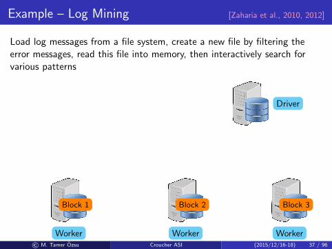
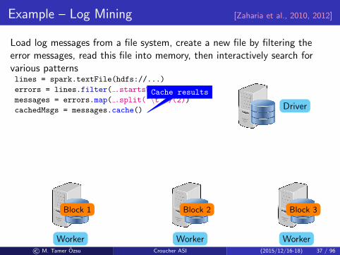
Load log messages from a file system, create a new file by filtering theerror messages, read this file into memory, then interactively search forvarious patterns
lines = spark.textFile(hdfs://...)
CreateRDD
errors = lines.filter( .startsWith(ERROR))
Transform RDD
messages = errors.map( .split(‘\t ’)(2))
Another transform
cachedMsgs = messages.cache()
Cache results
cachedMsgs.filter( .contains(foo)).count
Action
cachedMsgs.filter( .contains(bar)).count
Another Action
accesses cache
Driver
WorkerWorkerWorker
Block 1 Block 2 Block 3
TasksResults
Cache Cache Cache
© M. Tamer Ozsu Croucher ASI (2015/12/16-18) 37 / 96
Example – Log Mining [Zaharia et al., 2010, 2012]
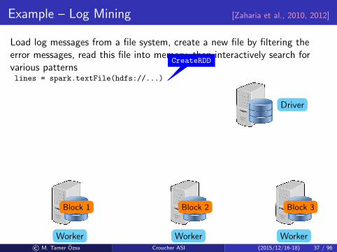
Load log messages from a file system, create a new file by filtering theerror messages, read this file into memory, then interactively search forvarious patternslines = spark.textFile(hdfs://...)
CreateRDD
errors = lines.filter( .startsWith(ERROR))
Transform RDD
messages = errors.map( .split(‘\t ’)(2))
Another transform
cachedMsgs = messages.cache()
Cache results
cachedMsgs.filter( .contains(foo)).count
Action
cachedMsgs.filter( .contains(bar)).count
Another Action
accesses cache
Driver
WorkerWorkerWorker
Block 1 Block 2 Block 3
TasksResults
Cache Cache Cache
© M. Tamer Ozsu Croucher ASI (2015/12/16-18) 37 / 96

Example – Log Mining [Zaharia et al., 2010, 2012]
Load log messages from a file system, create a new file by filtering theerror messages, read this file into memory, then interactively search forvarious patternslines = spark.textFile(hdfs://...)
CreateRDD
errors = lines.filter( .startsWith(ERROR))
Transform RDD
messages = errors.map( .split(‘\t ’)(2))
Another transform
cachedMsgs = messages.cache()
Cache results
cachedMsgs.filter( .contains(foo)).count
Action
cachedMsgs.filter( .contains(bar)).count
Another Action
accesses cache
Driver
WorkerWorkerWorker
Block 1 Block 2 Block 3
TasksResults
Cache Cache Cache
© M. Tamer Ozsu Croucher ASI (2015/12/16-18) 37 / 96

Example – Log Mining [Zaharia et al., 2010, 2012]
Load log messages from a file system, create a new file by filtering theerror messages, read this file into memory, then interactively search forvarious patternslines = spark.textFile(hdfs://...)
CreateRDD
errors = lines.filter( .startsWith(ERROR))
Transform RDD
messages = errors.map( .split(‘\t ’)(2))
Another transform
cachedMsgs = messages.cache()
Cache results
cachedMsgs.filter( .contains(foo)).count
Action
cachedMsgs.filter( .contains(bar)).count
Another Action
accesses cache
Driver
WorkerWorkerWorker
Block 1 Block 2 Block 3
Tasks
Results
Cache Cache Cache
© M. Tamer Ozsu Croucher ASI (2015/12/16-18) 37 / 96

Example – Log Mining [Zaharia et al., 2010, 2012]
Load log messages from a file system, create a new file by filtering theerror messages, read this file into memory, then interactively search forvarious patternslines = spark.textFile(hdfs://...)
CreateRDD
errors = lines.filter( .startsWith(ERROR))
Transform RDD
messages = errors.map( .split(‘\t ’)(2))
Another transform
cachedMsgs = messages.cache()
Cache results
cachedMsgs.filter( .contains(foo)).count
Action
cachedMsgs.filter( .contains(bar)).count
Another Action
accesses cache
Driver
WorkerWorkerWorker
Block 1 Block 2 Block 3
TasksResults
Cache Cache Cache
© M. Tamer Ozsu Croucher ASI (2015/12/16-18) 37 / 96

Example – Log Mining [Zaharia et al., 2010, 2012]
Load log messages from a file system, create a new file by filtering theerror messages, read this file into memory, then interactively search forvarious patternslines = spark.textFile(hdfs://...)
CreateRDD
errors = lines.filter( .startsWith(ERROR))
Transform RDD
messages = errors.map( .split(‘\t ’)(2))
Another transform
cachedMsgs = messages.cache()
Cache results
cachedMsgs.filter( .contains(foo)).count
Action
cachedMsgs.filter( .contains(bar)).count
Another Action
accesses cache
Driver
WorkerWorkerWorker
Block 1 Block 2 Block 3
TasksResults
Cache Cache Cache
© M. Tamer Ozsu Croucher ASI (2015/12/16-18) 37 / 96

RDD and Processing
HDFS
lines = spark.textFile(hdfs://...)
linesError, msg1
Warn, msg2
Error, msg1
Info, msg8
Warn, msg2
Info, msg8
Error, msg3
Info, msg5
Info, msg5
Error, msg4
Warn, msg9
Error, msg1
errors
errors = lines.filter( .startsWith(ERROR))
Error, msg1
Error, msg1
Error, msg3 Error, msg4
Error, msg1
messages
messages = errors.map .split(‘\t ’)(2)
msg1
msg1
msg3 msg4
msg1
Th
ese
are
no
tye
tg
ener
ated
© M. Tamer Ozsu Croucher ASI (2015/12/16-18) 38 / 96

RDD and Processing
lineserrors
messagesmsg1
msg1
msg3 msg4
msg1
lines
messages.filter( .contains(foo)).count
errors
messagesmsg1
msg1
msg3 msg4
msg1
Now
the
RD
Ds
are
mat
eria
lized
;
Co
mm
and
no
tye
tex
ecu
ted
Driver
messages.filter( .contains(foo)).count
© M. Tamer Ozsu Croucher ASI (2015/12/16-18) 38 / 96

GraphX [Gonzalez et al., 2014]
Built on top of Spark
Objective is to combine data analytics with graph processing
Unify computation on tables and graphs
Carefully convert graph to tabular representation
Native GraphX API or can accommodate vertex-centric computation
NativeSparkApps
SparkSQL
SparkStreaming
MLlib(machinelearning)
GraphX(graph
processing)
Apache Spark
Vertex-centric API
AppApp
App App
© M. Tamer Ozsu Croucher ASI (2015/12/16-18) 39 / 96

GraphX: Representation of Graphs as Tables
A
B
C
D
E
F
G
H
I
J
© M. Tamer Ozsu Croucher ASI (2015/12/16-18) 40 / 96

GraphX: Representation of Graphs as Tables
Partition 1
Partition 2
A
B
C
D
E
F
G
H
I
J
Edge-disjointpartitioning
© M. Tamer Ozsu Croucher ASI (2015/12/16-18) 40 / 96

GraphX: Representation of Graphs as Tables
Partition 1
Partition 2
Mac
hin
e1
Mac
hin
e2
Vertex Table
(RDD)v-prop:vertex prop.
A
B
C
D
E
F
G
H
I
J
Edge-disjointpartitioning
A v-prop
B v-prop
...
I v-prop
D v-prop
E v-prop
F v-prop
J v-prop
© M. Tamer Ozsu Croucher ASI (2015/12/16-18) 40 / 96

GraphX: Representation of Graphs as Tables
Partition 1
Partition 2
Mac
hin
e1
Mac
hin
e2
Vertex Table
(RDD)v-prop:vertex prop.
Edge Table
(RDD)e-prop:edge prop.
A
B
C
D
E
F
G
H
I
J
Edge-disjointpartitioning
A v-prop
B v-prop
...
I v-prop
D v-prop
E v-prop
F v-prop
J v-prop
A e-prop B
A e-prop C
...
F e-prop G
A e-prop D
A e-prop E...
E e-prop F
© M. Tamer Ozsu Croucher ASI (2015/12/16-18) 40 / 96

GraphX: Representation of Graphs as Tables
Partition 1
Partition 2
Mac
hin
e1
Mac
hin
e2
Vertex Table
(RDD)v-prop:vertex prop.
Edge Table
(RDD)e-prop:edge prop.
A
B
C
D
E
F
G
H
I
J
Edge-disjointpartitioning
A v-prop
B v-prop
...
I v-prop
D v-prop
E v-prop
F v-prop
J v-prop
A e-prop B
A e-prop C
...
F e-prop G
A e-prop D
A e-prop E...
E e-prop FJoining vertices
and edgesMove vertices to edges
© M. Tamer Ozsu Croucher ASI (2015/12/16-18) 40 / 96

GraphX: Representation of Graphs as Tables
Partition 1
Partition 2
Mac
hin
e1
Mac
hin
e2
Vertex Table
(RDD)v-prop:vertex prop.
Edge Table
(RDD)e-prop:edge prop.
RoutingTable
(RDD)
A
B
C
D
E
F
G
H
I
J
Edge-disjointpartitioning
A v-prop
B v-prop
...
I v-prop
D v-prop
E v-prop
F v-prop
J v-prop
A e-prop B
A e-prop C
...
F e-prop G
A e-prop D
A e-prop E...
E e-prop F
A 1 2
B 1
...
I 1
F 1 2
D 2
E 2
J 2
© M. Tamer Ozsu Croucher ASI (2015/12/16-18) 40 / 96

GraphX: Computation Model
Mac
hin
e1
Mac
hin
e2
Vertex Table Edge Table
A v-prop
B v-prop
...
I v-prop
D v-prop
E v-prop
F v-prop
J v-prop
A e-prop B
A e-prop C
...
F e-prop G
A e-prop D
A e-prop E...
E e-prop F
© M. Tamer Ozsu Croucher ASI (2015/12/16-18) 41 / 96

GraphX: Computation Model
Mac
hin
e1
Mac
hin
e2
Vertex Table Edge Table
A v-prop
B v-prop
...
I v-prop
D v-prop
E v-prop
F v-prop
J v-prop
A e-prop B
A e-prop C
...
F e-prop G
A e-prop D
A e-prop E...
E e-prop F
First Phase: JoinVertex table on Edge table
Triples View
A v-prop e-prop B v-prop
A v-prop e-prop C v-prop
C v-prop e-prop G v-prop
...
E v-prop e-prop G v-prop
J v-prop e-prop G v-prop
© M. Tamer Ozsu Croucher ASI (2015/12/16-18) 41 / 96

GraphX: Computation Model
Mac
hin
e1
Mac
hin
e2
Vertex Table Edge Table
A v-prop
B v-prop
...
I v-prop
D v-prop
E v-prop
F v-prop
J v-prop
A e-prop B
A e-prop C
...
F e-prop G
A e-prop D
A e-prop E...
E e-prop FTriples View
A v-prop e-prop B v-prop
A v-prop e-prop C v-prop
C v-prop e-prop G v-prop
...
E v-prop e-prop G v-prop
J v-prop e-prop G v-prop
Second Phase: Compute neighbourhoodGroup-by aggregate
© M. Tamer Ozsu Croucher ASI (2015/12/16-18) 41 / 96

GraphX: Operators
Table transform operators – inherited from Sparkmap(func) Return a new RDD formed by passing each element
of the source through a function func
filter(func) Return a new RDD formed by selecting thoseelements of the source on which func returns true
flatMap(func) Similar to map, but each input item can be mappedto 0 or more output items
mapPartitions(func) Similar to map, but runs separately on each partition(block) of the RDD, so func must be of type Iterator
sample(repl , fraction,seed)
Sample a fraction fraction of the data, with orwithout replacement (set repl accordingly), using agiven random number generator seed
union(otherDataset)intersection()
Return a new RDD containing the union/intersectionof the elements in the source RDD and the argument
groupByKey() Operates on a RDD of (K, V) pairs, returns a RDDof (K, Iterable<V>) pairs
reduceByKey(func, . . .) Operates on a RDD of (K, V) pairs, returns a RDDof (K, V) pairs where the values for each key areaggregated using the given reduce function func
Graph operatorsGraph(vertex coll ,edge coll)
Logically binds together a pair of vertex and edgeproperty collections into a property graph; verifiesthat each vertex occurs only once and edges connectexisting vertices
triplets(vertex coll ,vertex coll , edge coll)
Returns the triplets view of the graph
mrTriplets(map,reduce) MapReduce triplets - encodes the two-stage processof join to create triplets and group by
© M. Tamer Ozsu Croucher ASI (2015/12/16-18) 42 / 96

GraphX: Operators
Table transform operators – inherited from Spark
Graph operatorsGraph(vertex coll ,edge coll)
Logically binds together a pair of vertex and edgeproperty collections into a property graph; verifiesthat each vertex occurs only once and edges connectexisting vertices
triplets(vertex coll ,vertex coll , edge coll)
Returns the triplets view of the graph
mrTriplets(map,reduce) MapReduce triplets - encodes the two-stage processof join to create triplets and group by
© M. Tamer Ozsu Croucher ASI (2015/12/16-18) 42 / 96

Outline
1 Introduction – Graph Types
2 Property Graph ProcessingClassificationOnline queryingOffline analytics
3 RDF Graph QueryingData WarehousingDistributed SPARQL ExecutionLinked Object Data Querying
© M. Tamer Ozsu Croucher ASI (2015/12/16-18) 43 / 96

RDF Introduction
Everything is an uniquely namedresource
Prefixes can be used to shorten thenames
Properties of resources can be defined
Relationships with other resources canbe defined
Resource descriptions can becontributed by different people/groupsand can be located anywhere in the web
Integrated web “database”
http://data.linkedmdb.org/resource/actor/JN29704
xmlns:y=http://data.linkedmdb.org/resource/actor/
y:JN29704
y:JN29704:hasName “Jack Nicholson”
y:JN29704:BornOnDate “1937-04-22”
y:TS2014:title “The Shining”
y:TS2014:releaseDate “1980-05-23”
y:TS2014
JN29704:movieActor
© M. Tamer Ozsu Croucher ASI (2015/12/16-18) 44 / 96

RDF Data Model
Triple: Subject, Predicate (Property), Object(s, p, o)
Subject: the entity that is described (URIor blank node)
Predicate: a feature of the entity (URI)Object: value of the feature (URI, blank
node or literal)
(s, p, o) ∈ (U ∪ B)× U × (U ∪ B ∪ L)
Set of RDF triples is called an RDF graph
U
Subject Object
U B U B L
U: set of URIsB: set of blank nodesL: set of literals
Predicate
Subject Predicate Objecthttp://...imdb.../film/2014 rdfs:label “The Shining”http://...imdb.../film/2014 movie:releaseDate “1980-05-23”http://...imdb.../29704 movie:actor name “Jack Nicholson”. . . . . . . . .
© M. Tamer Ozsu Croucher ASI (2015/12/16-18) 45 / 96

RDF Example InstancePrefixes: mdb=http://data.linkedmdb.org/resource/; geo=http://sws.geonames.org/
bm=http://wifo5-03.informatik.uni-mannheim.de/bookmashup/lexvo=http://lexvo.org/id/;wp=http://en.wikipedia.org/wiki/
Subject Predicate Object
mdb: film/2014 rdfs:label “The Shining”mdb:film/2014 movie:initial release date “1980-05-23”’mdb:film/2014 movie:director mdb:director/8476mdb:film/2014 movie:actor mdb:actor/29704mdb:film/2014 movie:actor mdb: actor/30013mdb:film/2014 movie:music contributor mdb: music contributor/4110mdb:film/2014 foaf:based near geo:2635167mdb:film/2014 movie:relatedBook bm:0743424425mdb:film/2014 movie:language lexvo:iso639-3/engmdb:director/8476 movie:director name “Stanley Kubrick”mdb:film/2685 movie:director mdb:director/8476mdb:film/2685 rdfs:label “A Clockwork Orange”mdb:film/424 movie:director mdb:director/8476mdb:film/424 rdfs:label “Spartacus”mdb:actor/29704 movie:actor name “Jack Nicholson”mdb:film/1267 movie:actor mdb:actor/29704mdb:film/1267 rdfs:label “The Last Tycoon”mdb:film/3418 movie:actor mdb:actor/29704mdb:film/3418 rdfs:label “The Passenger”geo:2635167 gn:name “United Kingdom”geo:2635167 gn:population 62348447geo:2635167 gn:wikipediaArticle wp:United Kingdombm:books/0743424425 dc:creator bm:persons/Stephen+Kingbm:books/0743424425 rev:rating 4.7bm:books/0743424425 scom:hasOffer bm:offers/0743424425amazonOfferlexvo:iso639-3/eng rdfs:label “English”lexvo:iso639-3/eng lvont:usedIn lexvo:iso3166/CAlexvo:iso639-3/eng lvont:usesScript lexvo:script/Latn
URI Literal
URI
© M. Tamer Ozsu Croucher ASI (2015/12/16-18) 46 / 96

RDF Graph
mdb:film/2014
“1980-05-23”
movie:initial release date
“The Shining”refs:label
bm:books/0743424425
4.7
rev:rating
bm:offers/0743424425amazonOffer
geo:2635167
“United Kingdom”
gn:name
62348447
gn:population
mdb:actor/29704
“Jack Nicholson”
movie:actor name
mdb:film/3418
“The Passenger”
refs:label
mdb:film/1267
“The Last Tycoon”
refs:label
mdb:director/8476
“Stanley Kubrick”
movie:director name
mdb:film/2685
“A Clockwork Orange”
refs:label
mdb:film/424
“Spartacus”
refs:label
mdb:actor/30013
movie:relatedBook
scam:hasOffer
foaf:based nearmovie:actor
movie:directormovie:actor
movie:actor movie:actor
movie:director movie:director
© M. Tamer Ozsu Croucher ASI (2015/12/16-18) 47 / 96

RDF Query Model – SPARQL
Query Model - SPARQL Protocol and RDF Query LanguageGiven U (set of URIs), L (set of literals), and V (set of variables), aSPARQL expression is defined recursively:
an atomic triple pattern, which is an element of
(U ∪ V )× (U ∪ V )× (U ∪ V ∪ L)
?x rdfs:label “The Shining”
P FILTER R, where P is a graph pattern expression and R is a built-inSPARQL condition (i.e., analogous to a SQL predicate)
?x rev:rating ?p FILTER(?p > 3.0)
P1 AND/OPT/UNION P2, where P1 and P2 are graph patternexpressions
Example:SELECT ?nameWHERE {
?m r d f s : l a b e l ?name . ?m movie : d i r e c t o r ?d .?d movie : d i r e c t o r n a m e ” S t a n l e y K u b r i c k ” .?m movie : r e l a t e d B o o k ?b . ?b r e v : r a t i n g ? r .FILTER(? r > 4 . 0 )
}© M. Tamer Ozsu Croucher ASI (2015/12/16-18) 48 / 96

SPARQL Queries
SELECT ?nameWHERE {
?m r d f s : l a b e l ?name . ?m movie : d i r e c t o r ?d .?d movie : d i r e c t o r n a m e ” S t a n l e y K u b r i c k ” .?m movie : r e l a t e d B o o k ?b . ?b r e v : r a t i n g ? r .FILTER(? r > 4 . 0 )
}
?m ?dmovie:director
?name
rdfs:label
?b
movie:relatedBook
“Stanley Kubrick”
movie:director name
?rrev:rating
FILTER(?r > 4.0)
© M. Tamer Ozsu Croucher ASI (2015/12/16-18) 49 / 96

Outline
1 Introduction – Graph Types
2 Property Graph ProcessingClassificationOnline queryingOffline analytics
3 RDF Graph QueryingData WarehousingDistributed SPARQL ExecutionLinked Object Data Querying
© M. Tamer Ozsu Croucher ASI (2015/12/16-18) 50 / 96

Naıve Triple Store Design
SELECT ?nameWHERE {
?m r d f s : l a b e l ?name . ?m movie : d i r e c t o r ?d .?d movie : d i r e c t o r n a m e ” S t a n l e y K u b r i c k ” .?m movie : r e l a t e d B o o k ?b . ?b r e v : r a t i n g ? r .FILTER(? r > 4 . 0 )
}Subject Property Objectmdb:film/2014 rdfs:label “The Shining”mdb:film/2014 movie:initial release date “1980-05-23”mdb:film/2014 movie:director mdb:director/8476mdb:film/2014 movie:actor mdb:actor/29704mdb:film/2014 movie:actor mdb: actor/30013mdb:film/2014 movie:music contributor mdb: music contributor/4110mdb:film/2014 foaf:based near geo:2635167mdb:film/2014 movie:relatedBook bm:0743424425mdb:film/2014 movie:language lexvo:iso639-3/engmdb:director/8476 movie:director name “Stanley Kubrick”mdb:film/2685 movie:director mdb:director/8476mdb:film/2685 rdfs:label “A Clockwork Orange”mdb:film/424 movie:director mdb:director/8476mdb:film/424 rdfs:label “Spartacus”mdb:actor/29704 movie:actor name “Jack Nicholson”mdb:film/1267 movie:actor mdb:actor/29704mdb:film/1267 rdfs:label “The Last Tycoon”mdb:film/3418 movie:actor mdb:actor/29704mdb:film/3418 rdfs:label “The Passenger”geo:2635167 gn:name “United Kingdom”geo:2635167 gn:population 62348447geo:2635167 gn:wikipediaArticle wp:United Kingdombm:books/0743424425 dc:creator bm:persons/Stephen+Kingbm:books/0743424425 rev:rating 4.7bm:books/0743424425 scom:hasOffer bm:offers/0743424425amazonOfferlexvo:iso639-3/eng rdfs:label “English”lexvo:iso639-3/eng lvont:usedIn lexvo:iso3166/CAlexvo:iso639-3/eng lvont:usesScript lexvo:script/Latn
Easy to implementbut
too many self-joins!
© M. Tamer Ozsu Croucher ASI (2015/12/16-18) 51 / 96

Naıve Triple Store Design
SELECT ?nameWHERE {
?m r d f s : l a b e l ?name . ?m movie : d i r e c t o r ?d .?d movie : d i r e c t o r n a m e ” S t a n l e y K u b r i c k ” .?m movie : r e l a t e d B o o k ?b . ?b r e v : r a t i n g ? r .FILTER(? r > 4 . 0 )
}Subject Property Objectmdb:film/2014 rdfs:label “The Shining”mdb:film/2014 movie:initial release date “1980-05-23”mdb:film/2014 movie:director mdb:director/8476mdb:film/2014 movie:actor mdb:actor/29704mdb:film/2014 movie:actor mdb: actor/30013mdb:film/2014 movie:music contributor mdb: music contributor/4110mdb:film/2014 foaf:based near geo:2635167mdb:film/2014 movie:relatedBook bm:0743424425mdb:film/2014 movie:language lexvo:iso639-3/engmdb:director/8476 movie:director name “Stanley Kubrick”mdb:film/2685 movie:director mdb:director/8476mdb:film/2685 rdfs:label “A Clockwork Orange”mdb:film/424 movie:director mdb:director/8476mdb:film/424 rdfs:label “Spartacus”mdb:actor/29704 movie:actor name “Jack Nicholson”mdb:film/1267 movie:actor mdb:actor/29704mdb:film/1267 rdfs:label “The Last Tycoon”mdb:film/3418 movie:actor mdb:actor/29704mdb:film/3418 rdfs:label “The Passenger”geo:2635167 gn:name “United Kingdom”geo:2635167 gn:population 62348447geo:2635167 gn:wikipediaArticle wp:United Kingdombm:books/0743424425 dc:creator bm:persons/Stephen+Kingbm:books/0743424425 rev:rating 4.7bm:books/0743424425 scom:hasOffer bm:offers/0743424425amazonOfferlexvo:iso639-3/eng rdfs:label “English”lexvo:iso639-3/eng lvont:usedIn lexvo:iso3166/CAlexvo:iso639-3/eng lvont:usesScript lexvo:script/Latn
SELECT T1 . o b j e c tFROM T as T1 , T as T2 , T as T3 ,
T as T4 , T as T5WHERE T1 . p=” r d f s : l a b e l ”AND T2 . p=” movie : r e l a t e d B o o k ”AND T3 . p=” movie : d i r e c t o r ”AND T4 . p=” r e v : r a t i n g ”AND T5 . p=” movie : d i r e c t o r n a m e ”AND T1 . s=T2 . sAND T1 . s=T3 . sAND T2 . o=T4 . sAND T3 . o=T5 . sAND T4 . o > 4 . 0AND T5 . o=” S t a n l e y K u b r i c k ”
Easy to implementbut
too many self-joins!
© M. Tamer Ozsu Croucher ASI (2015/12/16-18) 51 / 96

Exhaustive Indexing
RDF-3X [Neumann and Weikum, 2008, 2009], Hexastore [Weisset al., 2008]
Strings are mapped to ids using a mapping table
Triples are indexed in a clustered B+ tree in lexicographic order
Create indexes for permutations of the three columns: SPO, SOP,PSO, POS, OPS, OSP
Original triple tableSubject Property Objectmdb: film/2014 rdfs:label “The Shining”mdb:film/2014 movie:initial release date “1980-05-23”mdb:director/8476 movie:director name “Stanley Kubrick”mdb:film/2685 movie:director mdb:director/8476
Encoded triple tableSubject Property Object
0 1 20 3 45 6 78 9 5
Mapping tableID Value0 mdb: film/20141 rdfs:label2 “The Shining”3 movie:initial release date4 “1980-05-23”5 mdb:director/84766 movie:director name7 “Stanley Kubrick”8 mdb:film/26859 movie:director
© M. Tamer Ozsu Croucher ASI (2015/12/16-18) 52 / 96

Exhaustive Indexing
RDF-3X [Neumann and Weikum, 2008, 2009], Hexastore [Weisset al., 2008]
Strings are mapped to ids using a mapping table
Triples are indexed in a clustered B+ tree in lexicographic order
Create indexes for permutations of the three columns: SPO, SOP,PSO, POS, OPS, OSP
Subject Property Object0 1 2
0 3 4
5 6 7
8 9 5...
......
B+ treeEasy queryingthrough mappingtable
© M. Tamer Ozsu Croucher ASI (2015/12/16-18) 52 / 96

Exhaustive Indexing–Query Execution
Each triple pattern can be answered by a range query
Joins between triple patterns computed using merge join
Join order is easy due to extensive indexing
Subject Property Object0 1 2
0 3 4
5 6 7
8 9 5...
......
ID Value0 mdb: film/2014
1 rdfs:label
2 “The Shining”
3 movie:initial release date
4 “1980-05-23”
5 mdb:director/8476
6 movie:director name
7 “Stanley Kubrick”
8 mdb:film/2685
9 movie:director
© M. Tamer Ozsu Croucher ASI (2015/12/16-18) 53 / 96

Exhaustive Indexing–Query Execution
Each triple pattern can be answered by a range query
Joins between triple patterns computed using merge join
Join order is easy due to extensive indexing
Subject Property Object0 1 2
0 3 4
5 6 7
8 9 5...
......
ID Value0 mdb: film/2014
1 rdfs:label
2 “The Shining”
3 movie:initial release date
4 “1980-05-23”
5 mdb:director/8476
6 movie:director name
7 “Stanley Kubrick”
8 mdb:film/2685
9 movie:director
Advantages
I Eliminates some of the joins – they become range queries
I Merge join is easy and fast
Disadvantages
I Space usage
© M. Tamer Ozsu Croucher ASI (2015/12/16-18) 53 / 96

Property Tables
Grouping by entities; Jena [Wilkinson, 2006], DB2-RDF [Borneaet al., 2013]
Clustered property table: group together the properties that tend tooccur in the same (or similar) subjects
Property-class table: cluster the subjects with the same type ofproperty into one property table
Subject Property Objectmdb:film/2014 rdfs:label “The Shining”mdb:film/2014 movie:director mdb:director/8476mdb:film/2685 movie:director mdb:director/8476mdb:film/2685 rdfs:label “A Clockwork Orange”mdb:actor/29704 movie:actor name “Jack Nicholson”. . . . . . . . .
Subject refs:label movie:directormob:film/2014 “The Shining” mob:director/8476mob:film/2685 “The Clockwork Orange” mob:director/8476
Subject movie:actor namemdb:actor “Jack Nicholson”
© M. Tamer Ozsu Croucher ASI (2015/12/16-18) 54 / 96

Property Tables
Grouping by entities; Jena [Wilkinson, 2006], DB2-RDF [Borneaet al., 2013]
Clustered property table: group together the properties that tend tooccur in the same (or similar) subjects
Property-class table: cluster the subjects with the same type ofproperty into one property table
Subject Property Objectmdb:film/2014 rdfs:label “The Shining”mdb:film/2014 movie:director mdb:director/8476mdb:film/2685 movie:director mdb:director/8476mdb:film/2685 rdfs:label “A Clockwork Orange”mdb:actor/29704 movie:actor name “Jack Nicholson”. . . . . . . . .
Subject refs:label movie:directormob:film/2014 “The Shining” mob:director/8476mob:film/2685 “The Clockwork Orange” mob:director/8476
Subject movie:actor namemdb:actor “Jack Nicholson”
Advantages
I Fewer joins
I If the data is structured, we have a relational system – similar tonormalized relations
Disadvantages
I Potentially a lot of NULLs
I Clustering is not trivial
I Multi-valued properties are complicated
© M. Tamer Ozsu Croucher ASI (2015/12/16-18) 54 / 96

Binary Tables
Grouping by properties: For each property, build a two-column table,containing both subject and object, ordered by subjects [Abadi et al.,2007, 2009]
Also called vertical partitioned tables
n two column tables (n is the number of unique properties in the data)
Subject Property Objectmdb:film/2014 rdfs:label “The Shining”mdb:film/2014 movie:director mdb:director/8476mdb:film/2685 movie:director mdb:director/8476mdb:film/2685 rdfs:label “A Clockwork Orange”mdb:actor/29704 movie:actor name “Jack Nicholson”. . . . . . . . .
Subject Objectmdb:film/2014 mdb:director/8476mdb:film/2685 mdb:director/8476
movie:director
Subject Objectmob:film/2014 “The Shining”mob:film/2685 “The Clockwork Orange”
refs:label
Subject Objectmdb:actor/29704 “Jack Nicholson”
movie:actor name
© M. Tamer Ozsu Croucher ASI (2015/12/16-18) 55 / 96

Binary Tables
Grouping by properties: For each property, build a two-column table,containing both subject and object, ordered by subjects [Abadi et al.,2007, 2009]
Also called vertical partitioned tables
n two column tables (n is the number of unique properties in the data)
Subject Property Objectmdb:film/2014 rdfs:label “The Shining”mdb:film/2014 movie:director mdb:director/8476mdb:film/2685 movie:director mdb:director/8476mdb:film/2685 rdfs:label “A Clockwork Orange”mdb:actor/29704 movie:actor name “Jack Nicholson”. . . . . . . . .
Subject Objectmdb:film/2014 mdb:director/8476mdb:film/2685 mdb:director/8476
movie:director
Subject Objectmob:film/2014 “The Shining”mob:film/2685 “The Clockwork Orange”
refs:label
Subject Objectmdb:actor/29704 “Jack Nicholson”
movie:actor name
Advantages
I Supports multi-valued properties
I No NULLs
I No clustering
I Read only needed attributes (i.e. less I/O)
I Good performance for subject-subject joins
Disadvantages
I Not useful for subject-object joins
I Expensive inserts
© M. Tamer Ozsu Croucher ASI (2015/12/16-18) 55 / 96

Graph-based Approach
Answering SPARQL query ≡ subgraph matching using homomorphism
gStore [Zou et al., 2011, 2014], chameleon-db [Aluc et al., 2013]
?m ?dmovie:director
?name
rdfs:label
?b
movie:relatedBook
“Stanley Kubrick”
movie:director name
?rrev:rating
FILTER(?r > 4.0)
mdb:film/2014
“1980-05-23”
movie:initial release date
“The Shining”refs:label
bm:books/0743424425
4.7
rev:rating
bm:offers/0743424425amazonOffer
geo:2635167
“United Kingdom”
gn:name
62348447
gn:population
mdb:actor/29704
“Jack Nicholson”
movie:actor name
mdb:film/3418
“The Passenger”
refs:label
mdb:film/1267
“The Last Tycoon”
refs:label
mdb:director/8476
“Stanley Kubrick”
movie:director name
mdb:film/2685
“A Clockwork Orange”
refs:label
mdb:film/424
“Spartacus”
refs:label
mdb:actor/30013
movie:relatedBook
scam:hasOffer
foaf:based nearmovie:actor
movie:directormovie:actor
movie:actor movie:actor
movie:director movie:director
SubgraphM
atching
© M. Tamer Ozsu Croucher ASI (2015/12/16-18) 56 / 96

Graph-based Approach
Answering SPARQL query ≡ subgraph matching using homomorphism
gStore [Zou et al., 2011, 2014], chameleon-db [Aluc et al., 2013]
?m ?dmovie:director
?name
rdfs:label
?b
movie:relatedBook
“Stanley Kubrick”
movie:director name
?rrev:rating
FILTER(?r > 4.0)
mdb:film/2014
“1980-05-23”
movie:initial release date
“The Shining”refs:label
bm:books/0743424425
4.7
rev:rating
bm:offers/0743424425amazonOffer
geo:2635167
“United Kingdom”
gn:name
62348447
gn:population
mdb:actor/29704
“Jack Nicholson”
movie:actor name
mdb:film/3418
“The Passenger”
refs:label
mdb:film/1267
“The Last Tycoon”
refs:label
mdb:director/8476
“Stanley Kubrick”
movie:director name
mdb:film/2685
“A Clockwork Orange”
refs:label
mdb:film/424
“Spartacus”
refs:label
mdb:actor/30013
movie:relatedBook
scam:hasOffer
foaf:based nearmovie:actor
movie:directormovie:actor
movie:actor movie:actor
movie:director movie:director
SubgraphM
atching
Advantages
I Maintains the graph structure
I Full set of queries can be handled
Disadvantages
I Graph pattern matching is expensive
© M. Tamer Ozsu Croucher ASI (2015/12/16-18) 56 / 96

Two Systems
gStore
mdb:film/2014
bm:books/0743424425
mdb:director/8476
mdb:film/424mdb:film/2685
mdb:actor/29804
mdb:film/3418 mdb:film/1267
mdb:actor/30013
movie:ac
tor
moive:director
“Spartacus”moive:director moive:director
“Jack_Nicholson”
“A Clockwork Orange”
rdfs:label
“1980-05-23”
rdfs:label
moive:actor_name
y:hasBudget
y:has_box_office
“22000000#dollar”
movie:relatedBook4.7
rev:rating
bm:offers/0743424425
scam:hasOffer
y:hasBudget y:hasBudget
“21000000#dollar” “26589355#dollar” “12000000#dollar” “60000000#dollar”
y:has_box_office
movie:actor
movie:actor movie:actor
“The Passager” “The last Tycoon”rdfs:label rdfs:label
“Scatman Crothers”
movie:initial_release_datemoive:actor_name
Fig. 2. An RDF graph G
?x
?y
?z
mdb:movierdf:type
moive:director
“*Jack*”moive:actor_name
y:hasBudget
?budget<30000000Desc, top10
movie:actor
SELECT ?x ?y WHERE{ ?x hasBudget ?budget. ?x rdf:type mdb:movie. ?x movie:director ?y. ?y movie:actor_name ?z. FILTER( regex(str(?z),``Jack'') AND (?budget <30000000) )}ORDER BY ?budgetLIMIT 10
Fig. 3. SPARQL and Query Graph Q
a query signature graph Q⇤, the encoding strategy is analogueto encoding RDF graphs.
The online query evaluation process consists of two steps:filtering and joining. First, we generate the candidates for eachquery node using VS⇤-tree. Then, applying a depth-first searchstrategy, we perform the multi-way join over these candidatelists to find the subgraph matches of SPARQL query Q overRDF graph G.
III. Techniques
In this section, we briefly discuss the techniques used ingStore system; full details are given in elsewhere [5], [6]. Ac-cording to our framework in Section II, we solve the SPARQLquery processing by subgraph matching over the signaturegraph. A key issue is that the proposed encoding and pruningstrategies should support, in a uniform manner, di↵erent kindsof data (such as strings and numeric data), and SPARQLqueries with di↵erent operators . We discuss the encoding andpruning methods in Section III-A. Another technical issue isthe index structure, which is discussed in Section III-B. Wealso present some system-oriented optimization, such as indexcaching strategy and multicore-based query optimization inour system.
A. Encoding Techniques
In gSore, answering SPARQL queries is equivalent tofinding subgraph matches of query graph Q over RDF graphG. If vertex v (in query Q) can match vertex u (in RDF graphG), each neighbor vertex and each adjacent edge of v shouldmatch to some neighbor vertex and some adjacent edge of u.Thus, given a vertex u in G, we encode each of its adjacentedge labels and the corresponding neighbor vertex labels into
System Architecture
Offline Online
Storage
Input Input
RDF Parser
RDF Graph Builder
Encoding Module
VS*-tree builder
RDF data
RDF Triples
RDF Graph
Signature Graph
Key-Value Store
VS*-treeStore
SPARQL Parser
SPARQL Query
Encoding Module
VS*-tree
Query Graph
Filter Module
Join Module
Signature Graph
Node Candidate
Results
Fig. 4. System Architecture
bitstrings, denoted as vS ig(u). We encode query Q with thesame encoding method. Consequently, the match between Qand G can be verified by simply checking the match betweencorresponding encoded bitstrings.
Given a vertex u, we encode each of its adjacent edgese(eLabel, nLabel) into a bitstring, where eLabel is the edgelabel and nLabel is the vertex label. This bitstring is callededge signature (i.e., eS ig(e)). It has two parts: eS ig(e).e,eS ig(e).n. The first part eS ig(e).e (M bits) denotes the edgelabel (i.e., eLabel) and the second part eS ig(e).n (N bits)denotes the neighbor vertex label (i.e., nLabel). The code ofvS ig(u) is formed by performing OR operator over all eS ig(e).Figure 5 illustrates the process.
mdb:film/2014
mdb:director/8476
mdb:actor/29804 moive:director
“1980-05-23”
y:hasBudget
“22000000#dollar”
movie:initial_release_date
movie:actor
e1 rdfs:label "The Shining"e2 movie:initial_release_date "1980-05-23"e3 movie:director mdb:director/8476e4 movie:actor mdb:actor/29704e5 movie:actor mdb:actor/30013e6 y:hasDuration 7140.0$#se7 y:hasBudget 22000000$#$e8 y:hasImdb "0081505"rdfs:label"The Shining"
hasDuration
hasDuration
"0081505"
y:hasImdb
eSig.e eSig.ne1 001000010 000010000101000e2 000110000 000000011100000e3 100100000 000010010000001e4 000010010 001001000000001e5 000010010 001001010000000e6 101000000 000001001100000e7 001010000 000010000001001e8 100010000 001000001001000
nSig 101110010 001011011101001
Fig. 5. Encoding Technique
1) Computing eS ig(e).e: Given an RDF repository, let |P|denote the number of di↵erent properties. If |P| is small, weset |eS ig(e).e| = |P|, where |eS ig(e).e| denotes the length ofthe bitstring, and build a 1-to-1 mapping between the propertyand the bit position. If |P| is large, we resort to the hashingtechnique. Let |eS ig(e).e| = M. Using an appropriate hashfunction, we set m out of M bits in eS ig(e).e to be ‘1’.
chameleon-db
Structural Index
...
Vertex Index
Spill Index
Clu
ster
Ind
ex
Sto
rag
eS
yst
em Sto
rag
eA
dvis
or
QueryEngine Plan Generation Evaluation
© M. Tamer Ozsu Croucher ASI (2015/12/16-18) 57 / 96

gStore
General Approach:
Work directly on the RDF graph and the SPARQL query graph
Use a signature-based encoding of each entity and class vertex tospeed up matching
Filter-and-evaluate
Use a false positive algorithm to prune nodes and obtain a set ofcandidates; then do more detailed evaluation on those
Use an index (VS∗-tree) over the data signature graph (has lightmaintenance load) for efficient pruning
© M. Tamer Ozsu Croucher ASI (2015/12/16-18) 58 / 96

1. Encode Q and G to Get Signature Graphs
Query signature graph Q∗
0100 0000 1000 000000010
0000 010010000
Data signature graph G∗
0010 1000
0100 0001
00001
1000 000100010
0000 0100
10000
0000 1000
10000
0000 0010
10000
0000 1001
00100
0001 000101000
0100 1000
01000
1001 1000
01000
0001 0100
01000
© M. Tamer Ozsu Croucher ASI (2015/12/16-18) 59 / 96

2. Filter-and-Evaluate
Query signature graph Q∗
0100 0000 1000 000000010
0000 010010000
Data signature graph G∗
0010 1000
0100 0001
00001
1000 000100010
0000 0100
10000
0000 1000
10000
0000 0010
10000
0000 1001
00100
0001 000101000
0100 1000
01000
1001 1000
01000
0001 0100
01000
Find matches of Q∗ oversignature graph G ∗
Verify each match inRDF graph G
© M. Tamer Ozsu Croucher ASI (2015/12/16-18) 60 / 96

How to Generate Candidate List
Two step process:1 For each node of Q∗ get lists of nodes in G∗ that include that node.2 Do a multi-way join to get the candidate list
Alternatives:
Sequential scan of G∗
Both steps are inefficient
Use S-trees
Height-balanced tree over signaturesRun an inclusion query for each node of Q∗ and get lists of nodes inG∗ that include that node.
• Given query signature q and a set of data signatures S , find alldata signatures si ∈ S where q&si = q
Does not support second step – expensive
VS-tree (and VS∗-tree)
Multi-resolution summary graph based on S-treeSupports both steps efficientlyGrouping by vertices
© M. Tamer Ozsu Croucher ASI (2015/12/16-18) 61 / 96

How to Generate Candidate List
Two step process:1 For each node of Q∗ get lists of nodes in G∗ that include that node.2 Do a multi-way join to get the candidate list
Alternatives:Sequential scan of G∗
Both steps are inefficient
Use S-trees
Height-balanced tree over signaturesRun an inclusion query for each node of Q∗ and get lists of nodes inG∗ that include that node.
• Given query signature q and a set of data signatures S , find alldata signatures si ∈ S where q&si = q
Does not support second step – expensive
VS-tree (and VS∗-tree)
Multi-resolution summary graph based on S-treeSupports both steps efficientlyGrouping by vertices
© M. Tamer Ozsu Croucher ASI (2015/12/16-18) 61 / 96

S-tree Solution
1111 1111
0110 1111 1101 1101
0000 1110 0110 1001 1100 1001 1001 1101
0000 1000
0000 0100 0000 0010
0010 1000
0100 0001
1000 0001
0000 1001
0100 1000
1001 1000
0001 0100
0001 0001
005
004 006
001
002
003
007
011
008
009
010
d11
d21 d2
2
d31 d3
2 d33 d3
4
G 3
G 2
G 1
1000 00000100 000000010
0000 010010000
Possibly large join space!
© M. Tamer Ozsu Croucher ASI (2015/12/16-18) 62 / 96

S-tree Solution
1111 1111
0110 1111 1101 1101
0000 1110 0110 1001 1100 1001 1001 1101
0000 1000
0000 0100 0000 0010
0010 1000
0100 0001
1000 0001
0000 1001
0100 1000
1001 1000
0001 0100
0001 0001
005
004 006
001
002
003
007
011
008
009
010
d11
d21 d2
2
d31 d3
2 d33 d3
4
G 3
G 2
G 1
1000 00000100 000000010
0000 010010000 002
011
003
008
004
009
Possibly large join space!
© M. Tamer Ozsu Croucher ASI (2015/12/16-18) 62 / 96

S-tree Solution
1111 1111
0110 1111 1101 1101
0000 1110 0110 1001 1100 1001 1001 1101
0000 1000
0000 0100 0000 0010
0010 1000
0100 0001
1000 0001
0000 1001
0100 1000
1001 1000
0001 0100
0001 0001
005
004 006
001
002
003
007
011
008
009
010
d11
d21 d2
2
d31 d3
2 d33 d3
4
G 3
G 2
G 1
1000 00000100 000000010
0000 010010000 002
011
003
008
004
009on on
Possibly large join space!
© M. Tamer Ozsu Croucher ASI (2015/12/16-18) 62 / 96
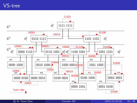
VS-tree
1111 1111
0110 1111 1101 1101
0000 1110 0110 1001 1100 1001 1001 1101
0000 1000
0000 0100 0000 0010
0010 1000
0100 0001
1000 0001
0000 1001
0100 1000
1001 1000
0001 0100
0001 0001
005
004 006
001
002
003
007
011
008
009
010
d11
d21 d2
2
d31 d3
2 d33 d3
4
G 3
G 2
G 1
11101
1001010001 01100
10000 00001 01100
00010
10000
01000
01000
10000
10000
10000
1000000010
00100
01000
01000
01000
01000
Super edge
© M. Tamer Ozsu Croucher ASI (2015/12/16-18) 63 / 96

Pruning with VS-Tree
1111 1111
0110 1111 1101 1101
0000 1110 0110 1001 1100 1001 1001 1101
0000 1000
0000 0100 0000 0010
0010 1000
0100 0001
1000 0001
0000 1001
0100 1000
1001 1000
0001 0100
0001 0001
005
004 006
001
002
003
007
011
008
009
010
d11
d21 d2
2
d31 d3
2 d33 d3
4
G 3
G 2
G 1
11101
1001010001 01100
10000 00001 01100
00010
10000
01000
01000
10000
10000
10000
1000000010
00100
01000
01000
01000
01000
1000 00000100 000000010
0000 010010000
d32
d33
d33
d34
d31
d34
G 3
00010 10000
01000
003
008
002
011
004
009onon
Reduced join space!
© M. Tamer Ozsu Croucher ASI (2015/12/16-18) 64 / 96

Adaptivity to Workload
Applications that rely on RDF data are increasingly popular and aremore varied [Verborgh et al., 2014]
Data that are being handled are far more heterogeneous [Duan et al.,2011]
SPARQL queries are becoming more diverse [Arias et al., 2011] anddynamic [Kirchberg et al., 2011]
An experiment [Aluc et al., 2014a]
No single system is a sole winner across all queriesNo single system is the sole loser across all queries, eitherThere can be 2–5 orders of magnitude difference in the performance(i.e., query execution time) between the best and the worst system fora given queryThe winner in one query may timeout in anotherPerformance difference widens as dataset size increases
© M. Tamer Ozsu Croucher ASI (2015/12/16-18) 65 / 96

Adaptivity to Workload
Applications that rely on RDF data are increasingly popular and aremore varied [Verborgh et al., 2014]
Data that are being handled are far more heterogeneous [Duan et al.,2011]
SPARQL queries are becoming more diverse [Arias et al., 2011] anddynamic [Kirchberg et al., 2011]
An experiment [Aluc et al., 2014a]
No single system is a sole winner across all queriesNo single system is the sole loser across all queries, eitherThere can be 2–5 orders of magnitude difference in the performance(i.e., query execution time) between the best and the worst system fora given queryThe winner in one query may timeout in anotherPerformance difference widens as dataset size increases
Can existing systems cope with these trends – workload diversity &dynamism
No! [Aluc et al., 2014b]
I Fragmented data
I Suboptimal pruning by indexes
I Unnecessarily large sets of intermediate result tuples
© M. Tamer Ozsu Croucher ASI (2015/12/16-18) 65 / 96

Adaptivity to Workload
Applications that rely on RDF data are increasingly popular and aremore varied [Verborgh et al., 2014]
Data that are being handled are far more heterogeneous [Duan et al.,2011]
SPARQL queries are becoming more diverse [Arias et al., 2011] anddynamic [Kirchberg et al., 2011]
An experiment [Aluc et al., 2014a]
No single system is a sole winner across all queriesNo single system is the sole loser across all queries, eitherThere can be 2–5 orders of magnitude difference in the performance(i.e., query execution time) between the best and the worst system fora given queryThe winner in one query may timeout in anotherPerformance difference widens as dataset size increases
Our proposal: Idea behind chameleon-db
I When designing and implementing an RDF data management system,assume nothing about the workload upfront
I Organize data dynamically and purely based on the workload
© M. Tamer Ozsu Croucher ASI (2015/12/16-18) 65 / 96

Group-by-Query Approach
v1
v21
A
v21
v20
B
v1
v98
A
v98
v30
C
v1
v250
A
v250
v40
D
v0
v32
A
v0
v52 C
v0
v80
C
v0
v66C
v0
v47
B
v6
v7
A
v6
v8
B
v6
v9
C
C1 C2 C3 C4 C5
Characteristics:
Records are not necessarily of fixed length
Records are not grouped into tables
Records do not necessarily share the same set of RDF predicates
Each record represents a very tiny part of the RDF graph
© M. Tamer Ozsu Croucher ASI (2015/12/16-18) 66 / 96
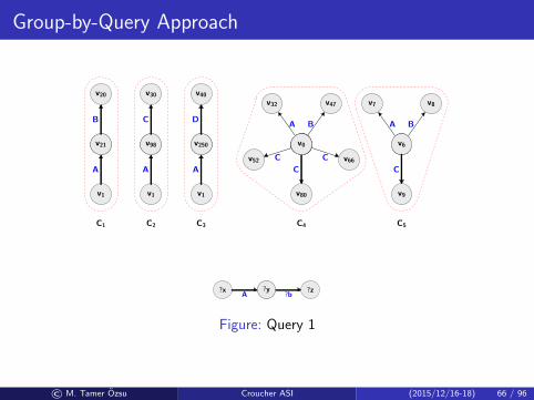
Group-by-Query Approach
v1
v21
A
v21
v20
B
v1
v98
A
v98
v30
C
v1
v250
A
v250
v40
D
v0
v32
A
v0
v52 C
v0
v80
C
v0
v66C
v0
v47
B
v6
v7
A
v6
v8
B
v6
v9
C
C1 C2 C3 C4 C5
?x ?yA
?y ?z?b
Figure: Query 1
© M. Tamer Ozsu Croucher ASI (2015/12/16-18) 66 / 96

Group-by-Query Approach
v1
v21
A
v21
v20
B
v1
v98
A
v98
v30
C
v1
v250
A
v250
v40
D
v0
v32
A
v0
v52 C
v0
v80
C
v0
v66C
v0
v47
B
v6
v7
A
v6
v8
B
v6
v9
C
C1 C2 C3 C4 C5
?x ?yA
?y ?z?b
Figure: Query 1
© M. Tamer Ozsu Croucher ASI (2015/12/16-18) 66 / 96
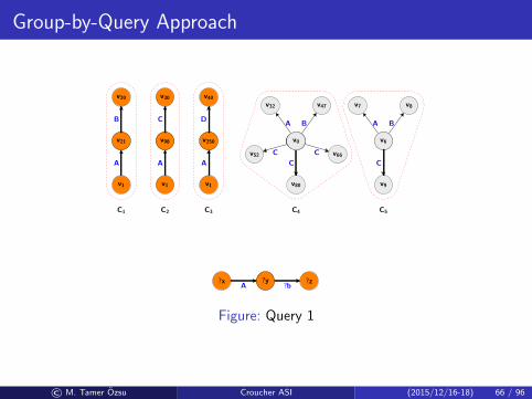
Group-by-Query Approach
v1
v21
A
v21
v20
B
v1
v98
A
v98
v30
C
v1
v250
A
v250
v40
D
v0
v32
A
v0
v52 C
v0
v80
C
v0
v66C
v0
v47
B
v6
v7
A
v6
v8
B
v6
v9
C
C1 C2 C3 C4 C5
?x ?yA
?y ?z?b
Figure: Query 1
© M. Tamer Ozsu Croucher ASI (2015/12/16-18) 66 / 96

Group-by-Query Approach
v1
v21
A
v21
v20
B
v1
v98
A
v98
v30
C
v1
v250
A
v250
v40
D
v0
v32
A
v0
v52 C
v0
v80
C
v0
v66C
v0
v47
B
v6
v7
A
v6
v8
B
v6
v9
C
C1 C2 C3 C4 C5
?a
?z
C
?a
?x
A
?a
?y
B
Figure: Query 2
© M. Tamer Ozsu Croucher ASI (2015/12/16-18) 66 / 96

Group-by-Query Approach
v1
v21
A
v21
v20
B
v1
v98
A
v98
v30
C
v1
v250
A
v250
v40
D
v0
v32
A
v0
v52 C
v0
v80
C
v0
v66C
v0
v47
B
v6
v7
A
v6
v8
B
v6
v9
C
C1 C2 C3 C4 C5
?a
?z
C
?a
?x
A
?a
?y
B
Figure: Query 2
© M. Tamer Ozsu Croucher ASI (2015/12/16-18) 66 / 96

Group-by-Query Approach
v1
v21
A
v21
v20
B
v1
v98
A
v98
v30
C
v1
v250
A
v250
v40
D
v0
v32
A
v0
v52 C
v0
v80
C
v0
v66C
v0
v47
B
v6
v7
A
v6
v8
B
v6
v9
C
C1 C2 C3 C4 C5
?a
?z
C
?a
?x
A
?a
?y
B
Figure: Query 2
© M. Tamer Ozsu Croucher ASI (2015/12/16-18) 66 / 96

Group-by-Query Approach
v1
v21
A
v21
v20
B
v1
v98
A
v98
v30
C
v1
v250
A
v250
v40
D
v0
v32
A
v0
v52 C
v0
v80
C
v0
v66C
v0
v47
B
v6
v7
A
v6
v8
B
v6
v9
C
C1 C2 C3 C4 C5
?a
?z
C
?a
?x
A
?a
?y
B
Figure: Query 2
Advantages
I Data are physically clustered for the workload
I Better pruning by the indexes
I Fewer intermediate result tuples
© M. Tamer Ozsu Croucher ASI (2015/12/16-18) 66 / 96

Challenges
Physical Data Layout: As the workloads change, the way data aregrouped together may no longer be suitable
Hierarchical Clustering Algorithm [Aluc et al., 2015]Tunable-LSH [Aluc et al., 2015]
Indexing: Indexing upfront is not a choice
Query Evaluation: Can we execute queries efficiently even when thephysical layout is constantly changing? [Aluc et al., 2015]
© M. Tamer Ozsu Croucher ASI (2015/12/16-18) 67 / 96

chameleon-db
Prototype system [Aluc et al., 2013]35,000 lines of code in C++ under Linux (plus code for SPARQL 1.0parser)
Structural Index
...
Vertex Index
Spill Index
Clu
ster
Inde
xS
tora
geS
yste
m Sto
rage
Adv
isor
QueryEngine Plan Generation Evaluation
© M. Tamer Ozsu Croucher ASI (2015/12/16-18) 68 / 96

Outline
1 Introduction – Graph Types
2 Property Graph ProcessingClassificationOnline queryingOffline analytics
3 RDF Graph QueryingData WarehousingDistributed SPARQL ExecutionLinked Object Data Querying
© M. Tamer Ozsu Croucher ASI (2015/12/16-18) 69 / 96

Remember the Environment
Distributed environment
Some of the data sites canprocess SPARQL queries –SPARQL endpoints
Not all data sites can processqueries
Alternatives
Data re-distribution + querydecompositionData re-distribution + partialevaluationSPARQL federation: justprocess at SPARQL endpointsLive querying (next section)
© M. Tamer Ozsu Croucher ASI (2015/12/16-18) 70 / 96

Remember the Environment
Distributed environment
Some of the data sites canprocess SPARQL queries –SPARQL endpoints
Not all data sites can processqueries
Alternatives
Data re-distribution + querydecomposition
Data re-distribution + partialevaluationSPARQL federation: justprocess at SPARQL endpointsLive querying (next section)
© M. Tamer Ozsu Croucher ASI (2015/12/16-18) 70 / 96

Remember the Environment
Distributed environment
Some of the data sites canprocess SPARQL queries –SPARQL endpoints
Not all data sites can processqueries
Alternatives
Data re-distribution + querydecompositionData re-distribution + partialevaluation
SPARQL federation: justprocess at SPARQL endpointsLive querying (next section)
© M. Tamer Ozsu Croucher ASI (2015/12/16-18) 70 / 96

Remember the Environment
Distributed environment
Some of the data sites canprocess SPARQL queries –SPARQL endpoints
Not all data sites can processqueries
Alternatives
Data re-distribution + querydecompositionData re-distribution + partialevaluationSPARQL federation: justprocess at SPARQL endpoints
Live querying (next section)
© M. Tamer Ozsu Croucher ASI (2015/12/16-18) 70 / 96

Remember the Environment
Distributed environment
Some of the data sites canprocess SPARQL queries –SPARQL endpoints
Not all data sites can processqueries
Alternatives
Data re-distribution + querydecompositionData re-distribution + partialevaluationSPARQL federation: justprocess at SPARQL endpointsLive querying (next section)
© M. Tamer Ozsu Croucher ASI (2015/12/16-18) 70 / 96

Distributed RDF Processing [Kaoudi and Manolescu, 2015]
RDF data warehouse is partitioned and distributedRDF data D = {D1, . . . ,Dn}Allocate each Di to a site
Partitioning alternativesTable-based (e.g., [Husain et al., 2011])Graph-based (e.g., [Huang et al., 2011; Zhang et al., 2013])Unit-based (e.g., [Gurajada et al., 2014; Lee and Liu, 2013])
SPARQL query decomposed Q = {Q1, . . . ,Qk}Distributed execution of {Q1, . . . ,Qk} over {D1, . . . ,Dn}
I High performance
I Great for parallelizing centralized RDF data
I May not be possible to re-partition and re-allocate Web data (i.e.,LOD)
I Query decomposition may not be easy
© M. Tamer Ozsu Croucher ASI (2015/12/16-18) 71 / 96

Distributed RDF Processing – 2
Data summary-based approaches
Build summaries (index) for the distributed RDF datasets (e.g., [Atreet al., 2010; Prasser et al., 2012])
SPARQL query Q = {Q1, . . . ,Qk}Distributed execution of {Q1, . . . ,Qk} using the data summary
I No data re-partitioning and re-allocation
I Have to scan the data at each site
I Index over distributed data with maintenance concerns
© M. Tamer Ozsu Croucher ASI (2015/12/16-18) 72 / 96

SPARQL Endpoint Federation
Consider only the SPARQL endpoints for query execution
No data re-partitioning/re-distribution
Consider D = D1 ∪ D2 ∪ . . . ∪ Dn; Di : SPARQL endpoint
SPARQL query decomposed Q = {Q1, . . . ,Qk}Distributed execution of {Q1, . . . ,Qk} over {D1, . . . ,Dn}Systems
DARQ, FedX [Schwarte et al., 2011], SPLENDID [Gorlitz and Staab,2011], ANAPSID [Acosta et al., 2011]
I Data integration approach
I May be the only way to proceed if data is distributed
I Not all RDF data storage points are SPARQL endpoints
© M. Tamer Ozsu Croucher ASI (2015/12/16-18) 73 / 96

SPARQL Endpoint Federation
Consider only the SPARQL endpoints for query execution
No data re-partitioning/re-distribution
Consider D = D1 ∪ D2 ∪ . . . ∪ Dn; Di : SPARQL endpoint
SPARQL query decomposed Q = {Q1, . . . ,Qk}Distributed execution of {Q1, . . . ,Qk} over {D1, . . . ,Dn}
Systems
DARQ, FedX [Schwarte et al., 2011], SPLENDID [Gorlitz and Staab,2011], ANAPSID [Acosta et al., 2011]
I Data integration approach
I May be the only way to proceed if data is distributed
I Not all RDF data storage points are SPARQL endpoints
© M. Tamer Ozsu Croucher ASI (2015/12/16-18) 73 / 96

SPARQL Endpoint Federation
Consider only the SPARQL endpoints for query execution
No data re-partitioning/re-distribution
Consider D = D1 ∪ D2 ∪ . . . ∪ Dn; Di : SPARQL endpoint
SPARQL query decomposed Q = {Q1, . . . ,Qk}Distributed execution of {Q1, . . . ,Qk} over {D1, . . . ,Dn}Systems
DARQ, FedX [Schwarte et al., 2011], SPLENDID [Gorlitz and Staab,2011], ANAPSID [Acosta et al., 2011]
I Data integration approach
I May be the only way to proceed if data is distributed
I Not all RDF data storage points are SPARQL endpoints
© M. Tamer Ozsu Croucher ASI (2015/12/16-18) 73 / 96

SPARQL Endpoint Federation
Consider only the SPARQL endpoints for query execution
No data re-partitioning/re-distribution
Consider D = D1 ∪ D2 ∪ . . . ∪ Dn; Di : SPARQL endpoint
SPARQL query decomposed Q = {Q1, . . . ,Qk}Distributed execution of {Q1, . . . ,Qk} over {D1, . . . ,Dn}Systems
DARQ, FedX [Schwarte et al., 2011], SPLENDID [Gorlitz and Staab,2011], ANAPSID [Acosta et al., 2011]
I Data integration approach
I May be the only way to proceed if data is distributed
I Not all RDF data storage points are SPARQL endpoints
© M. Tamer Ozsu Croucher ASI (2015/12/16-18) 73 / 96

Distributed SPARQL Using Partial Query Evaluation
Two steps:1 Evaluate a query at each site to find local matches
Query is the function and each Di is the known inputInner match or local partial match
2 Assemble the partial matches to get final resultCrossing matchCentralized assemblyDistributed assembly
D1
D2
D3
D4
Crossing match
© M. Tamer Ozsu Croucher ASI (2015/12/16-18) 74 / 96

Outline
1 Introduction – Graph Types
2 Property Graph ProcessingClassificationOnline queryingOffline analytics
3 RDF Graph QueryingData WarehousingDistributed SPARQL ExecutionLinked Object Data Querying
© M. Tamer Ozsu Croucher ASI (2015/12/16-18) 75 / 96

Linked Object Data – Closer Look
© M. Tamer Ozsu Croucher ASI (2015/12/16-18) 76 / 96

Globally Distributed Network of Data
© M. Tamer Ozsu Croucher ASI (2015/12/16-18) 77 / 96

Traditional Hypertext-based Web Access
IMDb WorldBook
Data exposedto the Webvia HTML
© M. Tamer Ozsu Croucher ASI (2015/12/16-18) 78 / 96

Linked Data Publishing Principles
IMDb WorldBook
(http://...linkedmdb.../Shining,releaseDate, 23 May 1980)(http://...linkedmdb.../Shining, filmLocation, http://cia.../UK)(http://...linkedmdb.../29704,actedIn, http://...linkedmdb.../Shining)
...
(http://cia.../UK, hasPopulation, 63230000)...
Shi
ning
UK
Data model: RDFGlobal identifier: URIAccess mechanism: HTTPConnection: data links
© M. Tamer Ozsu Croucher ASI (2015/12/16-18) 79 / 96

Live Query Processing
Not all data resides at SPARQLendpoints
Freshness of access to dataimportant
Potentially countably infinitedata sources
Live querying
On-line executionOnly rely on linked dataprinciples
Alternatives
Traversal-based approachesIndex-based approachesHybrid approaches
© M. Tamer Ozsu Croucher ASI (2015/12/16-18) 80 / 96

Linked Data Model [Hartig, 2012]
Web of Linked Data
Given a finite or countably infinite set D of Linked Documents, a Web ofLinked Data is a tuple W = (D, adoc, data) where:
I D ⊆ D,
I adoc is a partial mapping from URIs to D, and
I data is a total mapping from D to finite sets of RDF triples.
© M. Tamer Ozsu Croucher ASI (2015/12/16-18) 81 / 96

Linked Data Model [Hartig, 2012]
Web of Linked Data
Given a finite or countably infinite set D of Linked Documents, a Web ofLinked Data is a tuple W = (D, adoc, data) where:
I D ⊆ D,
I adoc is a partial mapping from URIs to D, and
I data is a total mapping from D to finite sets of RDF triples.
Data Links
A Web of Linked Data W = (D, adoc, data)contains a data link from document d ∈ D todocument d ′ ∈ D if there exists a URI u suchthat:
I u is mentioned in an RDF triplet ∈ data(d), and
I d ′ = adoc(u).© M. Tamer Ozsu Croucher ASI (2015/12/16-18) 81 / 96

SPARQL Query Semantics in Live Querying
Full-web semantics
Scope of evaluating a SPARQL expression is all Linked DataQuery result completeness cannot be guaranteed by any (terminating)execution
Reachability-based query semantics
Query consists of a SPARQL expression, a set of seed URIs S , and areachability condition cScope: all data along paths of data links that satisfy the conditionComputationally feasible
© M. Tamer Ozsu Croucher ASI (2015/12/16-18) 82 / 96

Traversal Approaches
Discover relevant URIs recursively bytraversing (specific) data links at queryexecution runtime [Hartig, 2013;Ladwig and Tran, 2011]
Implements reachability-based querysemantics
Start from a set of seed URIsRecursively follow and discover newURIs
Important issue is selection of seed URIs
Retrieved data serves to discover newURIs and to construct result
© M. Tamer Ozsu Croucher ASI (2015/12/16-18) 83 / 96

Traversal Approaches
Discover relevant URIs recursively bytraversing (specific) data links at queryexecution runtime [Hartig, 2013;Ladwig and Tran, 2011]
Implements reachability-based querysemantics
Start from a set of seed URIsRecursively follow and discover newURIs
Important issue is selection of seed URIs
Retrieved data serves to discover newURIs and to construct result
Advantages
Easy to implement.No data structure to maintain.
© M. Tamer Ozsu Croucher ASI (2015/12/16-18) 83 / 96
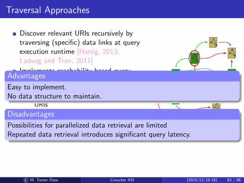
Traversal Approaches
Discover relevant URIs recursively bytraversing (specific) data links at queryexecution runtime [Hartig, 2013;Ladwig and Tran, 2011]
Implements reachability-based querysemantics
Start from a set of seed URIsRecursively follow and discover newURIs
Important issue is selection of seed URIs
Retrieved data serves to discover newURIs and to construct result
Advantages
Easy to implement.No data structure to maintain.
Disadvantages
Possibilities for parallelized data retrieval are limitedRepeated data retrieval introduces significant query latency.
© M. Tamer Ozsu Croucher ASI (2015/12/16-18) 83 / 96

Index Approaches
Use pre-populated index to determine relevant URIs (and to avoid asmany irrelevant ones as possible)
Different index keys possible; e.g., triple patterns [Umbrich et al.,2011]
Index entries a set of URIsIndexed URIs may appear multiple times (i.e., associated with multipleindex keys)Each URI in such an entry may be paired with a cardinality (utilized forsource ranking)
Key: tp Entry: {uri1, uri2, , urin}
GET urii
© M. Tamer Ozsu Croucher ASI (2015/12/16-18) 84 / 96

Index Approaches
Use pre-populated index to determine relevant URIs (and to avoid asmany irrelevant ones as possible)
Different index keys possible; e.g., triple patterns [Umbrich et al.,2011]
Index entries a set of URIsIndexed URIs may appear multiple times (i.e., associated with multipleindex keys)Each URI in such an entry may be paired with a cardinality (utilized forsource ranking)
Key: tp Entry: {uri1, uri2, , urin}
GET urii
Advantages
Data retrieval can be fully parallelizedReduces the impact of data retrieval on query execution time
Disadvantages
Querying can only start after index constructionDepends on what has been selected for the indexFreshness may be an issueIndex maintenance
© M. Tamer Ozsu Croucher ASI (2015/12/16-18) 84 / 96

Hybrid Approach
Perform a traversal-based execution using a prioritized list of URIs tolook up [Ladwig and Tran, 2010]
Initial seed from the pre-populated index
Non-seed URIs are ranked by a function based on information in theindex
New discovered URIs that are not in the index are ranked accordingto number of referring documents
© M. Tamer Ozsu Croucher ASI (2015/12/16-18) 85 / 96

Acknowledgements
This presentation draws upon collaborative research and discussions withthe following colleagues (in alphabetical order)
Gunes Aluc, U. Waterloo
Khaled Ammar, U. Waterloo
Khuzaima Daudjee, U. Waterloo
Young Han, U. Waterloo
Olaf Hartig, U. Waterloo
Lei Chen, Hong Kong UST
Lei Zou, Peking Univ.
© M. Tamer Ozsu Croucher ASI (2015/12/16-18) 86 / 96

Thank you!
Research supported by
© M. Tamer Ozsu Croucher ASI (2015/12/16-18) 87 / 96

© M. Tamer Ozsu Croucher ASI (2015/12/16-18) 88 / 96

References I
Abadi, D. J., Marcus, A., Madden, S., and Hollenbach, K. (2009). SW-Store: a verticallypartitioned DBMS for semantic web data management. VLDB J., 18(2):385–406.
Abadi, D. J., Marcus, A., Madden, S. R., and Hollenbach, K. (2007). Scalable semanticweb data management using vertical partitioning. In Proc. 33rd Int. Conf. on VeryLarge Data Bases, pages 411–422.
Acosta, M., Vidal, M.-E., Lampo, T., Castillo, J., and Ruckhaus, E. (2011). ANAPSID:an adaptive query processing engine for SPARQL endpoints. In Proc. 10th Int.Semantic Web Conf., pages 18–34.
Aluc, G., Ozsu, M. T., and Daudjee, K. (2015). Clustering RDF databases usingTunable-LSH. CoRR, abs/1504.02523.
Aluc, G., Hartig, O., Ozsu, M. T., and Daudjee, K. (2014a). Diversified stress testing ofRDF data management systems. In Proc. 13th Int. Semantic Web Conf., pages197–212.
Aluc, G., Ozsu, M. T., and Daudjee, K. (2014b). Workload matters: Why RDFdatabases need a new design. Proc. VLDB Endowment, 7(10):837–840.
© M. Tamer Ozsu Croucher ASI (2015/12/16-18) 89 / 96

References II
Aluc, G., Ozsu, M. T., Daudjee, K., and Hartig, O. (2013). chameleon-db: aworkload-aware robust RDF data management system. Technical Report CS-2013-10,University of Waterloo. Available at https://cs.uwaterloo.ca/sites/ca.computer-science/files/uploads/files/CS-2013-10.pdf.
Aluc, G., Ozsu, M. T., Daudjee, K., and Hartig, O. (2015). Executing queries overschemaless RDF databases. In Proc. 31st Int. Conf. on Data Engineering, pages807–818.
Ammar, K. and Ozsu, M. T. (2015). Approaches to graph processing – an overview. Inpreparation.
Arias, M., Fernandez, J. D., Martınez-Prieto, M. A., and de la Fuente, P. (2011). Anempirical study of real-world SPARQL queries. CoRR, abs/1103.5043.
Atre, M., Chaoji, V., Zaki, M. J., and Hendler, J. A. (2010). Matrix “bit” loaded: Ascalable lightweight join query processor for rdf data. In Proc. 19th Int. World WideWeb Conf., pages 41–50.
Bornea, M. A., Dolby, J., Kementsietsidis, A., Srinivas, K., Dantressangle, P., Udrea, O.,and Bhattacharjee, B. (2013). Building an efficient RDF store over a relationaldatabase. In Proc. ACM SIGMOD Int. Conf. on Management of Data, pages121–132.
© M. Tamer Ozsu Croucher ASI (2015/12/16-18) 90 / 96

References III
Bu, Y., Howe, B., Balazinska, M., and Ernst, M. D. (2012). The HaLoop approach tolarge-scale iterative data analysis. VLDB J., 21(2):169–190.
Dean, J. and Ghemawat, S. (2008). Mapreduce: Simplified data processing on largeclusters. Commun. ACM, 51(1):107–113.
Duan, S., Kementsietsidis, A., Srinivas, K., and Udrea, O. (2011). Apples and oranges:a comparison of RDF benchmarks and real RDF datasets. In Proc. ACM SIGMODInt. Conf. on Management of Data, pages 145–156.
Gonzalez, J. E., Xin, R. S., Dave, A., Crankshaw, D., Franklin, M. J., and Stoica, I.(2014). GraphX: graph processing in a distributed dataflow framework. In Proc. 11thUSENIX Symp. on Operating System Design and Implementation, pages 599–613.
Gorlitz, O. and Staab, S. (2011). SPLENDID: SPARQL endpoint federation exploitingVOID descriptions. In Proc. 2nd Int. Workshop on Consuming Linked Data.
Gurajada, S., Seufert, S., Miliaraki, I., and Theobald, M. (2014). TriAD: A distributedshared-nothing RDF engine based on asynchronous message passing. In Proc. ACMSIGMOD Int. Conf. on Management of Data, pages 289–300.
Han, M., Daudjee, K., Ammar, K., Ozsu, M. T., Wang, X., and Jin, T. (2014). Anexperimental comparison of Pregel-like graph processing systems. Proc. VLDBEndowment, 7(12):1047–1058.
© M. Tamer Ozsu Croucher ASI (2015/12/16-18) 91 / 96
References IV
Hartig, O. (2012). SPARQL for a web of linked data: Semantics and computability. InProc. 9th Extended Semantic Web Conf., pages 8–23.
Hartig, O. (2013). SQUIN: a traversal based query execution system for the web oflinked data. In Proc. ACM SIGMOD Int. Conf. on Management of Data, pages1081–1084.
Huang, J., Abadi, D. J., and Ren, K. (2011). Scalable SPARQL querying of large RDFgraphs. Proc. VLDB Endowment, 4(11):1123–1134.
Husain, M. F., McGlothlin, J., Masud, M. M., Khan, L. R., and Thuraisingham, B.(2011). Heuristics-based query processing for large RDF graphs using cloudcomputing. IEEE Trans. Knowl. and Data Eng., 23(9):1312–1327.
Kaoudi, Z. and Manolescu, I. (2015). RDF in the clouds: A survey. VLDB J., 24:67–91.
Kirchberg, M., Ko, R. K. L., and Lee, B.-S. (2011). From linked data to relevant data –time is the essence. CoRR, abs/1103.5046.
Ladwig, G. and Tran, T. (2010). Linked data query processing strategies. In Proc. 9thInt. Semantic Web Conf., pages 453–469.
Ladwig, G. and Tran, T. (2011). SIHJoin: Querying remote and local linked data. InProc. 8th Extended Semantic Web Conf., pages 139–153.
© M. Tamer Ozsu Croucher ASI (2015/12/16-18) 92 / 96

References V
Lee, K. and Liu, L. (2013). Scaling queries over big rdf graphs with semantic hashpartitioning. Proc. VLDB Endowment, 6(14):1894–1905.
Li, F., Ooi, B. C., Ozsu, M. T., and Wu, S. (2014). Distributed data management usingMapReduce. ACM Comput. Surv., 46(3):Article No. 31.
Low, Y., Gonzalez, J., Kyrola, A., Bickson, D., Guestrin, C., and Hellerstein, J. M.(2012). Distributed graphlab: A framework for machine learning in the cloud. Proc.VLDB Endowment, 5(8):716–727.
Malewicz, G., Austern, M. H., Bik, A. J. C., Dehnert, J. C., Horn, I., Leiser, N., andCzajkowski, G. (2010). Pregel: a system for large-scale graph processing. In Proc.ACM SIGMOD Int. Conf. on Management of Data, pages 135–146.
Michiardi, P. (2015). Introduction to spark internals. Slideshare. Available from:http://www.slideshare.net/michiard/introduction-to-spark-internals?
qid=511145e7-79d7-41d8-a133-9e705d4933c3&v=qf1&b=&from_search=11 [Lastretrieved: 9 July 2015].
Neumann, T. and Weikum, G. (2008). RDF-3X: a RISC-style engine for RDF. Proc.VLDB Endowment, 1(1):647–659.
© M. Tamer Ozsu Croucher ASI (2015/12/16-18) 93 / 96

References VI
Neumann, T. and Weikum, G. (2009). The RDF-3X engine for scalable management ofRDF data. VLDB J., 19(1):91–113.
Prasser, F., Kemper, A., and Kuhn, K. A. (2012). Efficient distributed query processingfor autonomous rdf databases. In Proc. 15th Int. Conf. on Extending DatabaseTechnology, pages 372–383.
Schwarte, A., Haase, P., Hose, K., Schenkel, R., and Schmidt, M. (2011). Fedx: Afederation layer for distributed query processing on linked open data. In Proc. 8thExtended Semantic Web Conf., pages 481–486.
Tian, Y., Balmin, A., Corsten, S. A., Tatikonda, S., and McPherson, J. (2013). From“think like a vertex” to “think like a graph”. Proc. VLDB Endowment, 7(3):193–204.
Umbrich, J., Hose, K., Karnstedt, M., Harth, A., and Polleres, A. (2011). Comparingdata summaries for processing live queries over linked data. World Wide Web J.,14(5-6):495–544.
Verborgh, R., Hartig, O., Meester, B. D., Haesendonck, G., Vocht, L. D., Sande, M. V.,Cyganiak, R., Colpaert, P., Mannens, E., and de Walle, R. V. (2014). Queryingdatasets on the web with high availability. In Proc. 13th Int. Semantic Web Conf.,pages 180–196.
© M. Tamer Ozsu Croucher ASI (2015/12/16-18) 94 / 96

References VII
Weiss, C., Karras, P., and Bernstein, A. (2008). Hexastore: sextuple indexing forsemantic web data management. Proc. VLDB Endowment, 1(1):1008–1019.
Wilkinson, K. (2006). Jena property table implementation. Technical ReportHPL-2006-140, HP Laboratories Palo Alto.
Yan, D., Cheng, J., Lu, Y., and Ng, W. (2014). Blogel: A block-centric framework fordistributed computation on real-world graphs. Proc. VLDB Endowment,7(14):1981–1992.
Zaharia, M. (2016). An Architecture for Fast and General Data Processing on LargeClusters. ACM Books. Forthcoming.
Zaharia, M., Chowdhury, M., Das, T., Dave, A., Ma, J., McCauley, M., Franklin, M. J.,Shenker, S., and Stoica, I. (2012). Resilient distributed datasets: A fault-tolerantabstraction for in-memory cluster computing. In Proc. 9th USENIX Symp. onNetworked Systems Design & Implementation, pages 2–2.
Zaharia, M., Chowdhury, M., Franklin, M. J., Shenker, S., and Stoica, I. (2010). Spark:Cluster computing with working sets. In Proc. 2nd USENIX Workshop on Hot Topicsin Cloud Computing, pages 10–10.
© M. Tamer Ozsu Croucher ASI (2015/12/16-18) 95 / 96

References VIII
Zhang, X., Chen, L., Tong, Y., and Wang, M. (2013). EAGRE: Towards scalable I/Oefficient SPARQL query evaluation on the cloud. In Proc. 29th Int. Conf. on DataEngineering, pages 565–576.
Zou, L., Mo, J., Chen, L., Ozsu, M. T., and Zhao, D. (2011). gStore: answeringSPARQL queries via subgraph matching. Proc. VLDB Endowment, 4(8):482–493.
Zou, L., Ozsu, M. T., Chen, L., Shen, X., Huang, R., and Zhao, D. (2014). gStore: Agraph-based SPARQL query engine. VLDB J., 23(4):565–590.
© M. Tamer Ozsu Croucher ASI (2015/12/16-18) 96 / 96