Embed Size (px)
Citation preview
Production & Operations Management Page 1
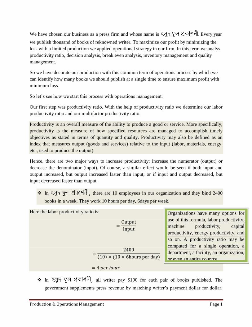
We have chosen our business as a press firm and whose name is . Every year
we publish thousand of books of reknowned writer. To maximize our profit by minimizing the
loss with a limited production we applied operational strategy in our firm. In this term we analys
productivity ratio, decision analysis, break even analysis, inventory management and quality
management.
So we have decorate our production with this common term of operations process by which we
can identify how many books we should publish at a single time to ensure maximum profit with
minimum loss.
So let’s see how we start this process with operations management.
Our first step was productivity ratio. With the help of productivity ratio we determine our labor
productivity ratio and our multifactor productivity ratio.
Productivity is an overall measure of the ability to produce a good or service. More specifically,
productivity is the measure of how specified resources are managed to accomplish timely
objectives as stated in terms of quantity and quality. Productivity may also be defined as an
index that measures output (goods and services) relative to the input (labor, materials, energy,
etc., used to produce the output).
Hence, there are two major ways to increase productivity: increase the numerator (output) or
decrease the denominator (input). Of course, a similar effect would be seen if both input and
output increased, but output increased faster than input; or if input and output decreased, but
input decreased faster than output.
In there are 10 employees in our organization and they bind 2400
books in a week. They work 10 hours per day, 6days per week.
Here the labor productivity ratio is:
=Output
Input
=2400
10 × (10 × 6hours per day)
= 4 𝑝𝑒𝑟 ℎ𝑜𝑢𝑟
In all writer pay $100 for each pair of books published. The
government supplements press revenue by matching writer’s payment dollar for dollar.
Organizations have many options for
use of this formula, labor productivity,
machine productivity, capital
productivity, energy productivity, and
so on. A productivity ratio may be
computed for a single operation, a
department, a facility, an organization,
or even an entire country.
Production & Operations Management Page 2
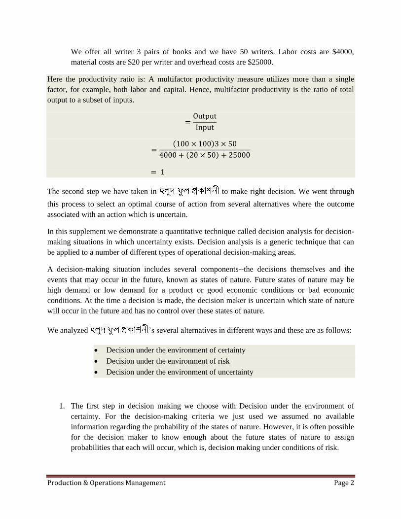
We offer all writer 3 pairs of books and we have 50 writers. Labor costs are $4000,
material costs are $20 per writer and overhead costs are $25000.
Here the productivity ratio is: A multifactor productivity measure utilizes more than a single
factor, for example, both labor and capital. Hence, multifactor productivity is the ratio of total
output to a subset of inputs.
=Output
Input
= 100 × 100 3 × 50
4000 + 20 × 50 + 25000
= 1
The second step we have taken in to make right decision. We went through
this process to select an optimal course of action from several alternatives where the outcome
associated with an action which is uncertain.
In this supplement we demonstrate a quantitative technique called decision analysis for decision-
making situations in which uncertainty exists. Decision analysis is a generic technique that can
be applied to a number of different types of operational decision-making areas.
A decision-making situation includes several components--the decisions themselves and the
events that may occur in the future, known as states of nature. Future states of nature may be
high demand or low demand for a product or good economic conditions or bad economic
conditions. At the time a decision is made, the decision maker is uncertain which state of nature
will occur in the future and has no control over these states of nature.
We analyzed ’s several alternatives in different ways and these are as follows:
Decision under the environment of certainty
Decision under the environment of risk
Decision under the environment of uncertainty
1. The first step in decision making we choose with Decision under the environment of
certainty. For the decision-making criteria we just used we assumed no available
information regarding the probability of the states of nature. However, it is often possible
for the decision maker to know enough about the future states of nature to assign
probabilities that each will occur, which is, decision making under conditions of risk.

Production & Operations Management Page 3
There are 3 ways to calculate decision making process under the environment of certainty and
these are as follows:
EMV(Expected Monetary Value)
EOL(Expected Opportunity Loss)
EVPI(Expected Value of Perfect Information)
So let’s see the anticipation through an illustration:
No of book copies sold
(in ten-thousand)
Probability
10 0.10
11 0.15
12 0.20
13 0.25
14 0.30
Cost of per copy is tk.30, sale price is tk.50. How many copies we should
publish we have to find it out.
So if we start with EMV our decision making process for stands with
as follows:
Possible
Demand
Probability Possible Stock Action
10 11 12 13 14
10
0.10 200 170 140 110 80
11
0.15 200 220 190 160 130
12
0.20 200 220 240 210 180
13
0.25 200 220 240 260 230
14
0.30 200 220 240 260 280
EMV=
200
215
222.5
220
205

Production & Operations Management Page 4
As the EMV is highest in 12(in ten thousand) copies of books will maximize monetary value
which is 222.5 (in millions), so we should go with this result.
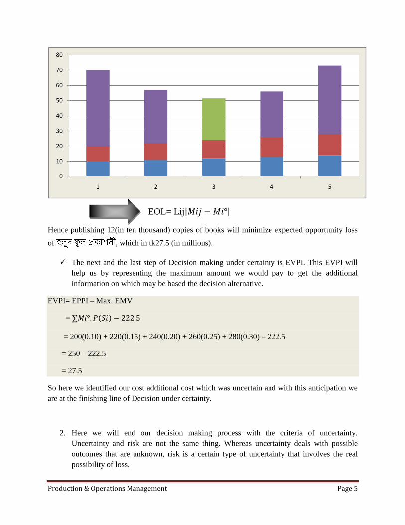
The next step is to find out the EOL and after finding it out our decision is as follows:
Possible
Demand
Probability Possible Stock Action
10 11 12 13 14
10
0.10 0 30 60 90 120
11
0.15 20 0 30 60 90
12
0.20 40 20 0 30 60
13
0.25 60 40 20 0 30
14
0.30 80 60 40 20 0
EOL=
50
35
27.5
30
45
185
190
195
200
205
210
215
220
225
1 2 3 4 5
Production & Operations Management Page 5
EOL= Lij 𝑀𝑖𝑗 − 𝑀𝑖°
Hence publishing 12(in ten thousand) copies of books will minimize expected opportunity loss
of , which in tk27.5 (in millions).
The next and the last step of Decision making under certainty is EVPI. This EVPI will
help us by representing the maximum amount we would pay to get the additional
information on which may be based the decision alternative.
EVPI= EPPI – Max. EMV
= ∑𝑀𝑖°. 𝑃 𝑆𝑖 − 222.5
= 200(0.10) + 220(0.15) + 240(0.20) + 260(0.25) + 280(0.30) – 222.5
= 250 – 222.5
= 27.5
So here we identified our cost additional cost which was uncertain and with this anticipation we
are at the finishing line of Decision under certainty.
2. Here we will end our decision making process with the criteria of uncertainty.
Uncertainty and risk are not the same thing. Whereas uncertainty deals with possible
outcomes that are unknown, risk is a certain type of uncertainty that involves the real
possibility of loss.
0
10
20
30
40
50
60
70
80
1 2 3 4 5
Production & Operations Management Page 6
Uncertainty is a state of having limited knowledge of current conditions or future
outcomes. It is a major component of risk, which involves the likelihood and scale of
negative consequences. Managers often deal with uncertainty in their work; to minimize
the risk that their decisions will lead to undesired outcomes, they must develop the skills
and judgment necessary for reducing this uncertainty. Managing uncertainty and risk also
involves mitigating or even removing things that inhibit effective decision-making or
adversely affect performance.
One cause of uncertainty is proximity: things that are about to happen are easier to
estimate than those further out in the future. One approach to dealing with uncertainty is
to put off decisions until data become more accessible and reliable. Of course, delaying
some decisions can bring its own set of risks, especially when the potential negative
consequences of waiting are great.
Under uncertainty criteria we are going to discuss following process and these are as follows:
Maximax or optimistic
Maximin or pessimistic
Equally likely probability or Laplace
Minimax or regret
Hurwicz criterion
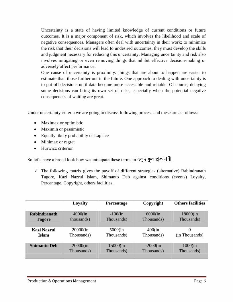
So let’s have a broad look how we anticipate these terms in .
The following matrix gives the payoff of different strategies (alternative) Rabindranath
Tagore, Kazi Nazrul Islam, Shimanto Deb against conditions (events) Loyalty,
Percentage, Copyright, others facilities.
Loyalty Percentage Copyright Others facilities
Rabindranath
Tagore
4000(in
thousands)
-100(in
Thousands)
6000(in
Thousands)
18000(in
Thousands)
Kazi Nazrul
Islam
20000(in
Thousands)
5000(in
Thousands)
400(in
Thousands)
0
(in Thousands)
Shimanto Deb
20000(in
Thousands)
15000(in
Thousands)
-2000(in
Thousands)
1000(in
Thousands)

Production & Operations Management Page 7
Now the decision taken under the following approaches:
Alternatives
Maximax Maximin Equal Likelihood
Rabindranath
Tagore
18000(in
Thousands)
-100(in
Thousands)
14 4000 − 100 + 6000
+ 18000 = 6975(in Thousands)
Kazi Nazrul Islam 20000(in
Thousands)
0 14 20000 + 5000 + 400 + 0
= 6350(in Thousands)
Shimanto Deb 20000(in
Thousands)
-2000(in
Thousands)
14 2000 + 15000 − 2000
+ 1000 = 8500(in Thousands)
a) Under Maximax or Optimistic criterion Kazi Nazrul Islam & Shimanto Deb is the
optimal act.
b) Under Maximin or Pessimistic criterion Kazi Nazrul Islam is the optimal act.
17000
17500
18000
18500
19000
19500
20000
20500
Tagore Nazrul Shimanto
Series1
-2500
-2000
-1500
-1000
-500
0
Tagore Nazrul Shimanto
Series1
Production & Operations Management Page 8
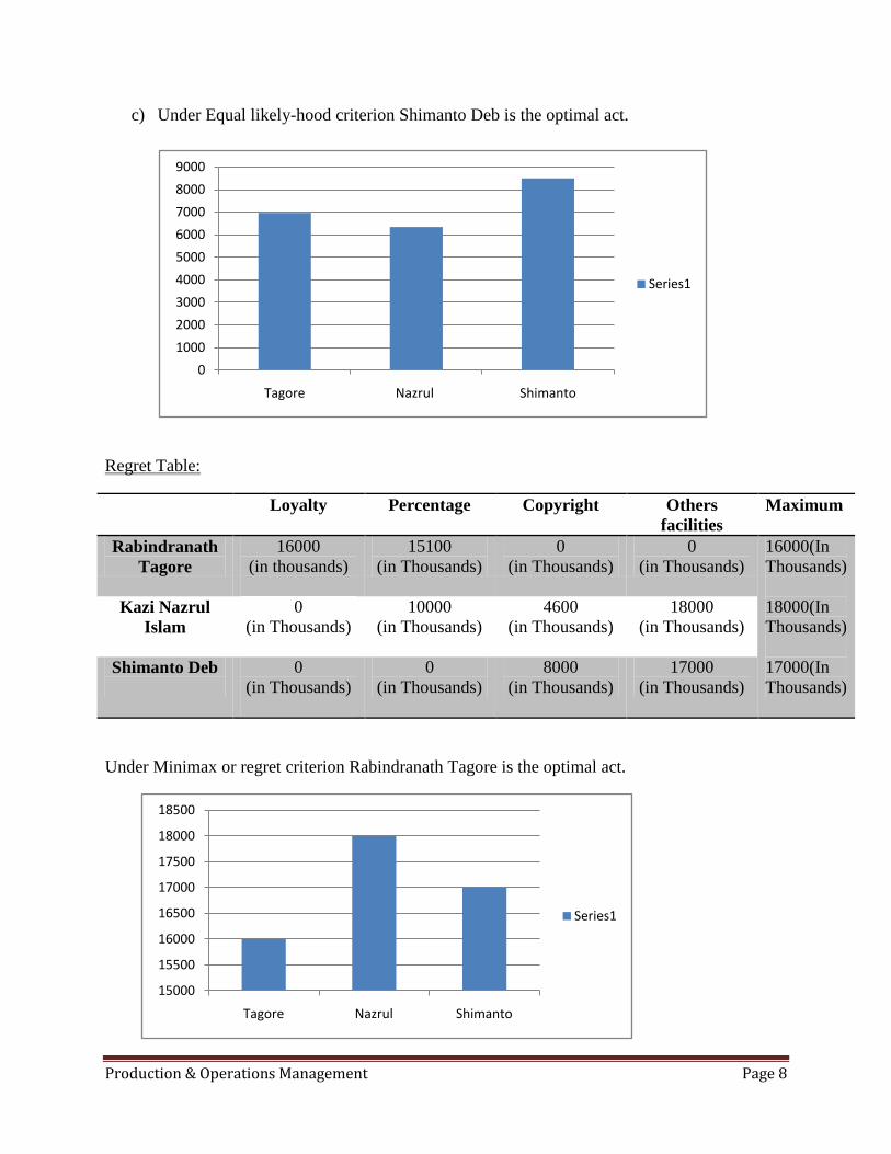
c) Under Equal likely-hood criterion Shimanto Deb is the optimal act.
Regret Table:
Loyalty Percentage Copyright Others
facilities
Maximum
Rabindranath
Tagore
16000
(in thousands)
15100
(in Thousands)
0
(in Thousands)
0
(in Thousands)
16000(In
Thousands)
18000(In
Thousands)
17000(In
Thousands)
Kazi Nazrul
Islam
0
(in Thousands)
10000
(in Thousands)
4600
(in Thousands)
18000
(in Thousands)
Shimanto Deb
0
(in Thousands)
0
(in Thousands)
8000
(in Thousands)
17000
(in Thousands)
Under Minimax or regret criterion Rabindranath Tagore is the optimal act.
15000
15500
16000
16500
17000
17500
18000
18500
Tagore Nazrul Shimanto
Series1
0
1000
2000
3000
4000
5000
6000
7000
8000
9000
Tagore Nazrul Shimanto
Series1
Production & Operations Management Page 9
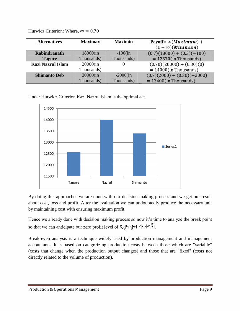
Hurwicz Criterion: Where, ∞ = 0.70
Alternatives
Maximax Maximin Payoff= ∞ 𝑴𝒂𝒙𝒊𝒎𝒖𝒎 + 𝟏 − ∞ (𝑴𝒊𝒏𝒊𝒎𝒖𝒎)
Rabindranath
Tagore
18000(in
Thousands)
-100(in
Thousands)
0.7 18000 + 0.3 −100
= 12570(in Thousands)
Kazi Nazrul Islam 20000(in
Thousands)
0 0.70 20000 + 0.30 0 = 14000(in Thousands)
Shimanto Deb 20000(in
Thousands)
-2000(in
Thousands)
0.7 2000 + 0.30 −2000 = 13400(in Thousands)
Under Hurwicz Criterion Kazi Nazrul Islam is the optimal act.
By doing this approaches we are done with our decision making process and we get our result
about cost, loss and profit. After the evaluation we can undoubtedly produce the necessary unit
by maintaining cost with ensuring maximum profit.
Hence we already done with decision making process so now it’s time to analyze the break point
so that we can anticipate our zero profit level of .
Break-even analysis is a technique widely used by production management and management
accountants. It is based on categorizing production costs between those which are "variable"
(costs that change when the production output changes) and those that are "fixed" (costs not
directly related to the volume of production).
11500
12000
12500
13000
13500
14000
14500
Tagore Nazrul Shimanto
Series1
Production & Operations Management Page 10
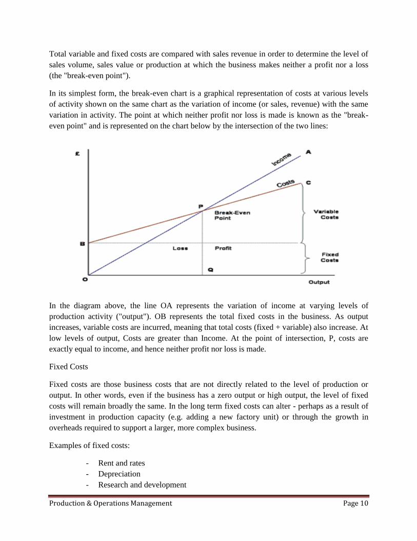
Total variable and fixed costs are compared with sales revenue in order to determine the level of
sales volume, sales value or production at which the business makes neither a profit nor a loss
(the "break-even point").
In its simplest form, the break-even chart is a graphical representation of costs at various levels
of activity shown on the same chart as the variation of income (or sales, revenue) with the same
variation in activity. The point at which neither profit nor loss is made is known as the "break-
even point" and is represented on the chart below by the intersection of the two lines:
In the diagram above, the line OA represents the variation of income at varying levels of
production activity ("output"). OB represents the total fixed costs in the business. As output
increases, variable costs are incurred, meaning that total costs (fixed + variable) also increase. At
low levels of output, Costs are greater than Income. At the point of intersection, P, costs are
exactly equal to income, and hence neither profit nor loss is made.
Fixed Costs
Fixed costs are those business costs that are not directly related to the level of production or
output. In other words, even if the business has a zero output or high output, the level of fixed
costs will remain broadly the same. In the long term fixed costs can alter - perhaps as a result of
investment in production capacity (e.g. adding a new factory unit) or through the growth in
overheads required to support a larger, more complex business.
Examples of fixed costs:
- Rent and rates
- Depreciation
- Research and development
Production & Operations Management Page 11
- Marketing costs (non- revenue related)
- Administration costs
Variable Costs
Variable costs are those costs which vary directly with the level of output. They represent
payment output-related inputs such as raw materials, direct labour, fuel and revenue-related costs
such as commission.
A distinction is often made between "Direct" variable costs and "Indirect" variable costs.
Direct variable costs are those which can be directly attributable to the production of a particular
product or service and allocated to a particular cost centre. Raw materials and the wages those
working on the production line are good examples.
Indirect variable costs cannot be directly attributable to production but they do vary with output.
These include depreciation maintenance and certain labor costs.
Here we represent our anticipation by an illustration, so let’s have a look on it.
is trying to determine how best to publish its e-book system. The e-
book could be published in our own press using either process A or process B. Cost data
are given bellow.
Fixed Cost
Variable Cost
Process A 15000
3
Process B 10000
5
Here,
Fa= 15000 Fb= 10000
Va= 3 Vb= 5
The break even quantity stands for
Vaq + Fa = Vbq + Fb
Vaq − Vbq = Fb − Fa
q Vb − Va = Fb − Fa

Production & Operations Management Page 12
q = Fb−Fa
(Va−Vb )
q = 10000−15000
3−5
q = 2500
Breakeven point analysis:
𝑉𝑎𝑞 + 𝐹𝑎
= 3 × 2500 + 15000
= 7500 + 15000
= 22500
𝑉𝑏𝑞 + 𝐹𝑏
= 5 × 2500 + 10000
= 12500 + 10000
= 22500
2500
22500
BEP
a b
Production & Operations Management Page 13
Here the breakeven cost is 22500 & the breakeven quantity is 2500.
Now it’s time to anticipate the inventory management in . So we have divided
our investigation in three approaches and these are as follows:
EOQ model with static demand
EOQ model with non instantaneous receipt
Quality discount with constant carrying cost
Economic order quantity (EOQ) is an equation for inventory that determines the ideal order
quantity a company should purchase for its inventory given a set cost of production, demand
rate and other variables. This is done to minimize variable inventory costs, and the formula
takes into account storage, or holding, costs, ordering costs and shortage costs. The full
equation is as follows:
2𝑘𝐷 ∕ ℎ
Where,
K = Ordering-costs
D = Demand
h = Holding-cost
Here,
Demand of books (D) = 50unit/day
Setup cost of books (k) = 20/order
Holding cost of books (h) = o.05/day
Lead time for publishing books = 7days
Le of publishing books = 3days
s EOQ are as follows:
i. Optimum order quantity (y) 2𝑘𝐷 ∕ ℎ
2 × 20 × 50 ∕ 0.05
200 𝑢𝑛𝑖𝑡𝑠
ii. Associated cycle length (t𝑦
𝐷)
𝑦
𝐷
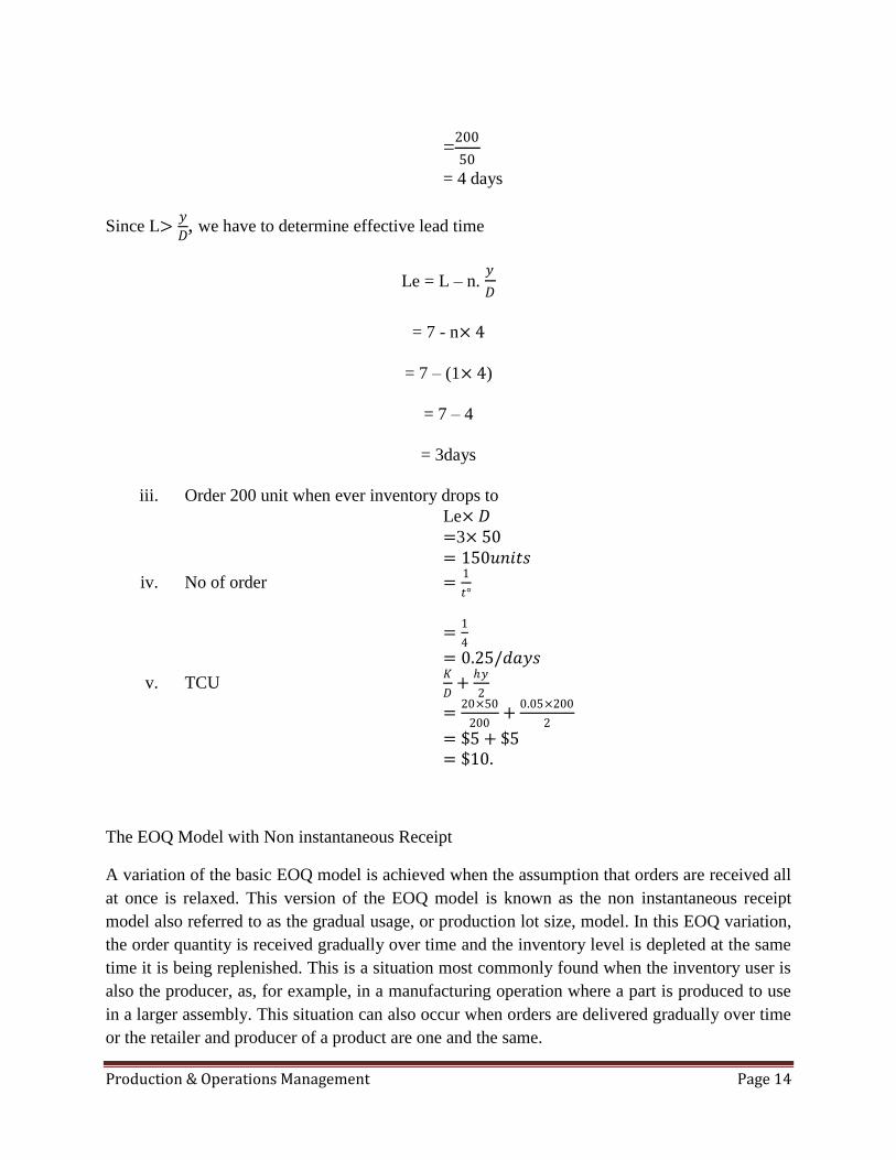
Production & Operations Management Page 14
=200
50
= 4 days
Since L>𝑦
𝐷, we have to determine effective lead time
Le = L – n. 𝑦
𝐷
= 7 - n× 4
= 7 – (1× 4)
= 7 – 4
= 3days
iii. Order 200 unit when ever inventory drops to
Le× 𝐷
=3× 50
= 150𝑢𝑛𝑖𝑡𝑠
iv. No of order =1
𝑡°
=1
4
= 0.25/𝑑𝑎𝑦𝑠
v. TCU 𝐾
𝐷+
ℎ𝑦
2
=20×50
200+
0.05×200
2
= $5 + $5
= $10.
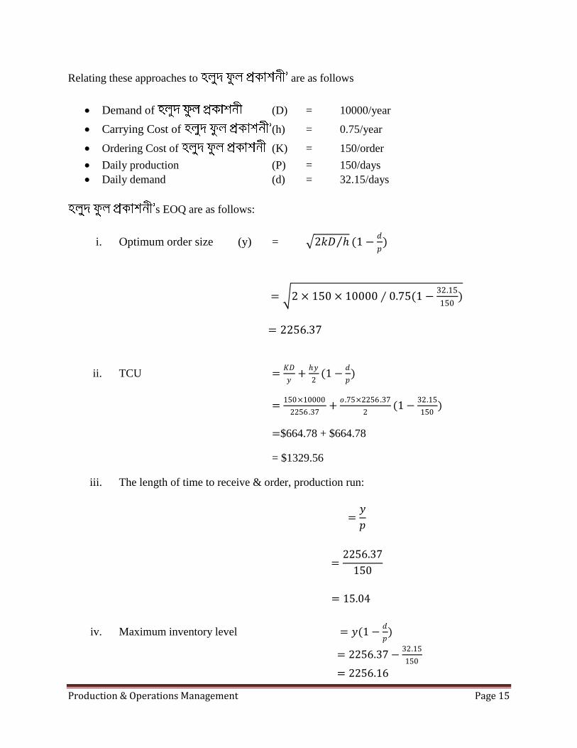
The EOQ Model with Non instantaneous Receipt
A variation of the basic EOQ model is achieved when the assumption that orders are received all
at once is relaxed. This version of the EOQ model is known as the non instantaneous receipt
model also referred to as the gradual usage, or production lot size, model. In this EOQ variation,
the order quantity is received gradually over time and the inventory level is depleted at the same
time it is being replenished. This is a situation most commonly found when the inventory user is
also the producer, as, for example, in a manufacturing operation where a part is produced to use
in a larger assembly. This situation can also occur when orders are delivered gradually over time
or the retailer and producer of a product are one and the same.
Production & Operations Management Page 15
Relating these approaches to are as follows
Demand of (D) = 10000/year
Carrying Cost of (h) = 0.75/year
Ordering Cost of (K) = 150/order
Daily production (P) = 150/days
Daily demand (d) = 32.15/days
s EOQ are as follows:
i. Optimum order size (y) = 2𝑘𝐷 ℎ (1 −𝑑
𝑝)
= 2 × 150 × 10000 ∕ 0.75(1 −32.15
150)
= 2256.37
ii. TCU =𝐾𝐷
𝑦+
ℎ𝑦
2(1 −
𝑑
𝑝)
=150×10000
2256 .37+
𝑜 .75×2256.37
2(1 −
32.15
150)
=$664.78 + $664.78
= $1329.56
iii. The length of time to receive & order, production run:
=𝑦
𝑝
=2256.37
150
= 15.04
iv. Maximum inventory level = 𝑦(1 −𝑑
𝑝)
= 2256.37 −32.15
150
= 2256.16
Production & Operations Management Page 16
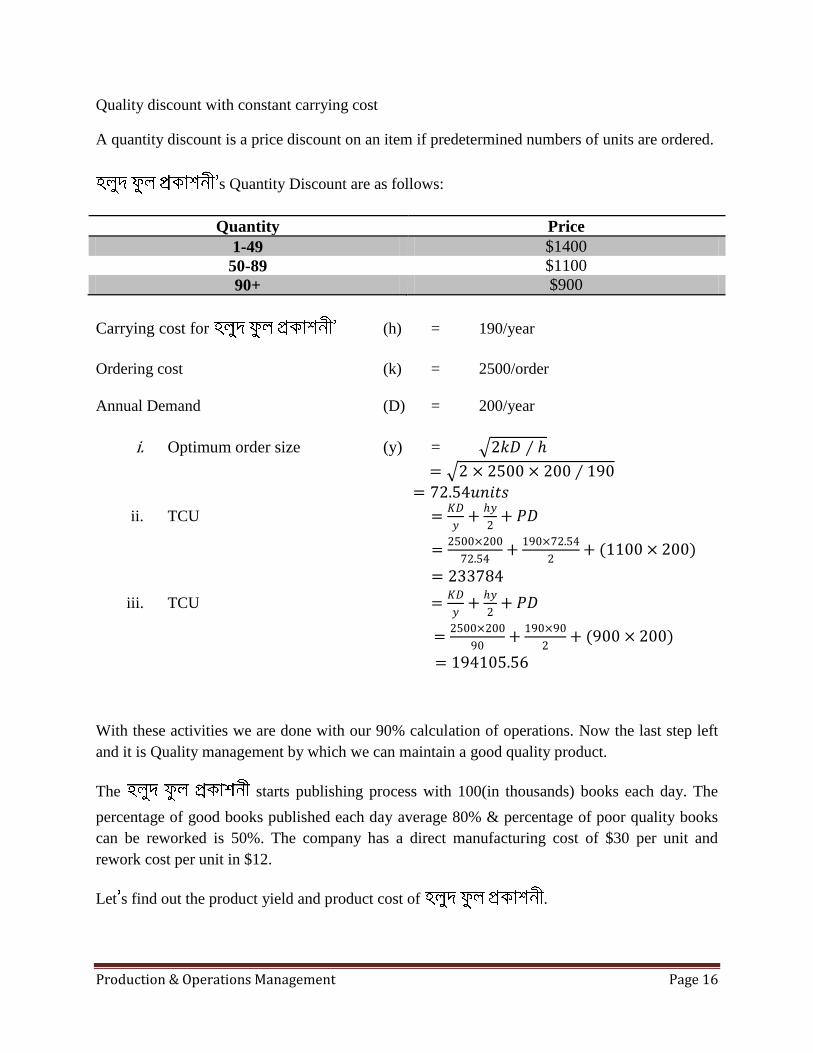
Quality discount with constant carrying cost
A quantity discount is a price discount on an item if predetermined numbers of units are ordered.
s Quantity Discount are as follows:
Quantity Price
1-49 $1400
50-89 $1100
90+ $900
Carrying cost for (h) = 190/year
Ordering cost (k) = 2500/order
Annual Demand (D) = 200/year
i. Optimum order size (y) = 2𝑘𝐷 ∕ ℎ
= 2 × 2500 × 200 ∕ 190 = 72.54𝑢𝑛𝑖𝑡𝑠
ii. TCU =𝐾𝐷
𝑦+
ℎ𝑦
2+ 𝑃𝐷
=2500×200
72.54+
190×72.54
2+ (1100 × 200)
= 233784
iii. TCU =𝐾𝐷
𝑦+
ℎ𝑦
2+ 𝑃𝐷
=2500×200
90+
190×90
2+ (900 × 200)
= 194105.56
With these activities we are done with our 90% calculation of operations. Now the last step left
and it is Quality management by which we can maintain a good quality product.
The starts publishing process with 100(in thousands) books each day. The
percentage of good books published each day average 80% & percentage of poor quality books
can be reworked is 50%. The company has a direct manufacturing cost of $30 per unit and
rework cost per unit in $12.
Let s find out the product yield and product cost of .
Production & Operations Management Page 17
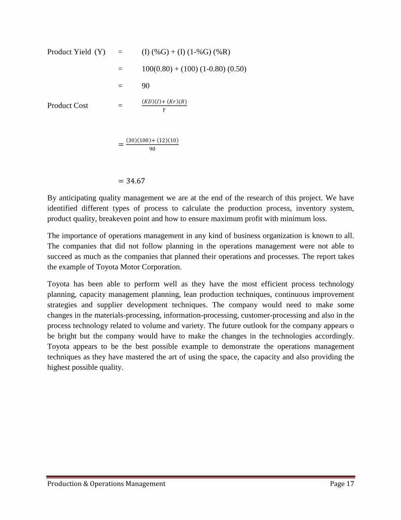
Product Yield (Y) = (I) (%G) + (I) (1-%G) (%R)
= 100(0.80) + (100) (1-0.80) (0.50)
= 90
Product Cost = 𝐾𝐷 𝐼 + 𝐾𝑟 (𝑅)
𝑌
= 30 100 + 12 10
90
= 34.67
By anticipating quality management we are at the end of the research of this project. We have
identified different types of process to calculate the production process, inventory system,
product quality, breakeven point and how to ensure maximum profit with minimum loss.
The importance of operations management in any kind of business organization is known to all.
The companies that did not follow planning in the operations management were not able to
succeed as much as the companies that planned their operations and processes. The report takes
the example of Toyota Motor Corporation.
Toyota has been able to perform well as they have the most efficient process technology
planning, capacity management planning, lean production techniques, continuous improvement
strategies and supplier development techniques. The company would need to make some
changes in the materials-processing, information-processing, customer-processing and also in the
process technology related to volume and variety. The future outlook for the company appears o
be bright but the company would have to make the changes in the technologies accordingly.
Toyota appears to be the best possible example to demonstrate the operations management
techniques as they have mastered the art of using the space, the capacity and also providing the
highest possible quality.


![Firm Profile 0620.ppt [Read-Only] · (Firm Registration No. 102511W/Wl00298) whose term completes as Statutory Auditors of the Company at the conclusion of ensuing Twenty Sixth Annual](https://img.pdfslide.us/doc/110x75/5f0642ca7e708231d4171a79/firm-profile-0620ppt-read-only-firm-registration-no-102511wwl00298-whose.jpg)