JFD

The role of a biometrician in an

International Agricultural Center:

service and research in an

interdisciplinary frame

Some ideas and examples

JFD

Interdisciplinary collaboration

• No man (or woman) is an island

• Few problems are simple problems

• Problems are better solved using teams of specialists working together

• The biometrician needs scientist’s data to propose and test methodologies and the scientists need the analytical tools to address their problems

JFD

Should be possible for the Biometrician to

participate in all or some of

• Planning of surveys and experiments

• Data processing, analysis and interpretation

• Design of novel tools/methodologies for analysis

• Writing and/or editing results

• Seminars and courses on new methodologies

and software (the free software issue)

• Capacity building (internal and external)

JFD

Trying to

• Allow researchers to work in depth within

their disciplines and problems, not on

methods for data analysis, computer

routines, software, etc.

• Supply new points of view and new

methodological tools on the research work

• Improve the quality of inferences

JFD

Four levels of participation

1. Routine analysis and known problems: short

and fast responses

2. New problems, known methodologies: we

need think together

3. New problems, existing methodology: we need

to understand, study and propose solutions

4. New problems, unknown methodology: we

need do some methodological research

JFD

Some examples of

interdisciplinary collaboration

JFD

Experimental Design

(continuous traits, Mixed Model)

• Spatial analysis of an Experimental Design

• Variety trial designed as a row-column design

with 64 varieties planted in two contiguous

replicates laid out in 8 rows and 16 columns

Nguyen and Williams, 1993

(Austral. J. Stat. 35: 363-370)

JFD

Layout (r=2, t=64)

-lattice (0,1,2)

r

e

p

r

o

wcolumn

1 2 3 4 5 6 7 8 9 10 11 12 13 14 15 16

1 1 5 19 55 23 27 38 64 44 14 13 59 25 45 49 11 43

1 2 2 36 62 29 34 40 52 54 28 26 58 42 32 6 39 53

1 3 37 3 17 24 15 50 47 56 16 30 31 60 7 18 8 21

1 4 20 35 57 63 46 12 41 10 22 1 51 61 33 48 4 9

2 5 58 44 15 25 18 53 5 22 55 36 33 29 12 47 8 1

2 6 41 17 63 37 38 19 26 21 28 4 6 45 56 46 59 42

2 7 14 9 62 48 34 31 60 13 20 7 64 3 39 40 10 23

2 8 24 52 11 54 51 57 35 2 50 27 30 61 43 49 32 16

5,3 = 0 5,2 = 1 5,44 = 2

JFD

Statistical models

ijkljljkjiij

ijjiij

y

y

)()(

Local control of field heterogeneity

RCBD

Row-Col

JFD

1...0000

..................

0...1000

0...0100

0...0010

0...0001

2R

• Assumptions on the “error” RV: V( ) = 2R

1...)()(

............

)(...1)(

)(...)(1

21

221

112

2

nn

n

n

dfdf

dfdf

dfdf

R

Repeated measures

Spatial analysis

Usual GLM:

Independence

dij: distance in time and/or space

JFD

three distance functions f(d i j )

0.00

0.50

1.00

0 10 20 30 40 50

distance

f(d

)

spherical exponential gaussian

JFD

Spatial statistical modelentry

Where:

i = 1,2,…, t (entries)

j = 1,2,…, J (replications)

k = 1,2,.., K (rows)

l = 1,2,…, L (columns)

),0(~ RN

y ijkliijkl

ε

JFD

ResultsPrecision of estimates and test of hypothesis

Average Standard Error of ls-means

rcbd row-col spat-sph

Average 0.5076 0.4041 0.4526

Standard Errors of some ls-means differences

Label rcbd row-col spat-sph

5 vs 3 0 0.7179 0.5256 0.4737

5 vs 2 1 0.7179 0.4833 0.4286

5 vs 14 2 0.7179 0.5232 0.4906

5 vs 44 2 0.7179 0.5159 0.4938

JFD

conclusion

When possible it is convenient to use

layouts that allow the spatial analysis with

the objective of reaching lower standard

errors for the contrasts

JFD

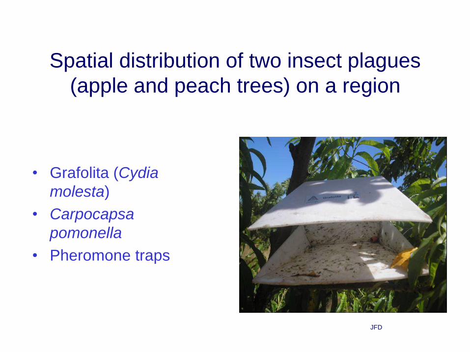
Spatial distribution of two insect plagues

(apple and peach trees) on a region

• Grafolita (Cydia

molesta)

• Carpocapsa

pomonella

• Pheromone traps

JFD

Objectives

• To obtain regionalized maps of the spatial distribution of an insect plague across time and on the whole crop growth stage

• Define the “convenient” distance between (pheromone) traps

• Software: SAS, S+, GS+, GIS software, R?

JFD

traps location

(25 x 26 km)

JFD

Semivariogram (geostatistics)

1000

1200

1400

1600

1800

2000

2200

2400

2600

0 5000 10000 15000

distance (m)

se

miv

ar

Sill point

Range

Nugget (intercept)

JFD

1)(

)(

:

)(

:

)(5.05.11)(

:

2

2

3

ii

d

ij

d

ij

ij

ijij

ij

df

df

Gaussian

df

lExponentia

dIdd

df

Spherical

e

e

ij

ij

(range): distance from which observations are independent

JFD

A linear mixed model is used to

selecting the best fit model, and

estimating the range

ijijy)}({

)( 2

ijdfF

FRV

JFD

• Null model: the independence model

R0=2I, in which ij = 0 for all ij

• Alternative model: the spatially related model:

R = 2F,

F={f(dij)} matrix

• Using a Likelihood Ratio Test (LRT)

JFD

Results

Model -2 Log(L) (1) -2 log( ) P( 2 > 2c)

Carpocapsa

Independence 1169

Spherical 4818 1156 12.7 0.002 **

Gaussian 2256 1157 11.9 0.003 **

Exponential 1343 1157 11.8 0.003 **

Grafolita

independence 1785

Spherical 1290 1782 3.5 0.174 ns

Gaussian 604 1781 4.0 0.135 ns

Exponential 527 1780 4.6 0.100 ns

)(ˆ m

(1) smaller -2Log(L) is better

JFD

Prediction (interpolation)

Prediction of non observed values using the

observed values plus the knowledge of a good

spatial model: KRIGING procedures

Krige, Danie G. (1951). "A statistical approach to some basic mine

valuation problems on the Witwatersrand". J. of the Chem., Metal.

and Mining Soc. of South Africa 52 (6): 119–139.

JFD

Mean Standard

deviation

Range Number of traps

60 49 6-259 111

Carpocapsa

JFD

Forecasting

(a more complex model)

• Forest inventory and growth models

– Non linear (but linearized models)

– structured equations models

JFD

Growth forestry model

• Eucalyptus (Bicostata)

• In a region

• Using the inventory data sets (yearly data)

• n = 2461

- from 506 plots (300 m2, circular)

- Measured each year (from 3 to 15)

• “difference” models

JFD

First data set

(coefficient estimation and model fit)

nplot Y1 Y2 H1 H2 BA1 BA2 N1 N2 V1 V2 S

100 3 4 12.5 16.9 15.7 22.2 1367 1367 53.2 108.0 22.3

100 4 5 16.9 17.7 22.2 26.1 1367 1367 108.0 135.9 24.2

100 5 6 17.7 22.9 26.1 30.3 1367 1367 135.9 183.9 21.7

100 6 7 22.9 23.3 30.3 33.2 1367 1333 183.9 219.3 25.0

100 7 8 23.3 23.3 33.2 36.6 1333 1333 219.3 244.9 23.3

100 8 9 23.3 23.9 36.6 38.2 1333 1333 244.9 264.6 21.7

100 9 10 23.9 24.1 38.2 39.7 1333 1333 264.6 275.7 21.1

100 10 11 24.1 25.7 39.7 41.7 1333 1333 275.7 304.9 20.3

100 11 12 25.7 25.0 41.7 46.4 1333 1333 304.9 327.0 20.9

JFD

An external equation

(dominant height and site index)

2

)exp(1

)exp(1

11

2112

A

Ahh

2ˆ

11

11

)ˆexp(1

)7ˆexp(1

AhS

JFD

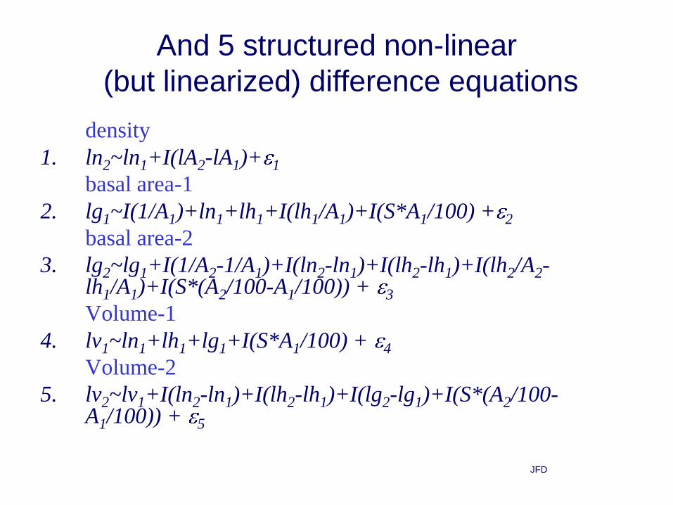
And 5 structured non-linear

(but linearized) difference equations

density

1. ln2~ln1+I(lA2-lA1)+ 1

basal area-1

2. lg1~I(1/A1)+ln1+lh1+I(lh1/A1)+I(S*A1/100) + 2

basal area-2

3. lg2~lg1+I(1/A2-1/A1)+I(ln2-ln1)+I(lh2-lh1)+I(lh2/A2-lh1/A1)+I(S*(A2/100-A1/100)) + 3

Volume-1

4. lv1~ln1+lh1+lg1+I(S*A1/100) + 4

Volume-2

5. lv2~lv1+I(ln2-ln1)+I(lh2-lh1)+I(lg2-lg1)+I(S*(A2/100-A1/100)) + 5

JFD

characteristics

• results from an equation are independent variables on another

• “residuals” ( 1, 2,…, 5) are correlated and, possibly, do not have homogeneous variances

• it is necessary a simultaneous estimation process

• 22 regression coefficients

• Possible methods: OLS, SUR, 2SLS, 3SLS

• Software: Systemfit in “R” (freeware)

JFD

model

evaluation

Internal:

Model fit on a randomly

selected sub-dataset

External:

adjust of estimated model

on other “independent”

sub-dataset

Year by year Long term

JFD

Second data set: forecasting

(prediction and external fit)nplot Y1 Y2 HD1 BA1 N1 V1 S

100 3 4 12.5 15.74 1366.7 53.2 22.3

100 3 5 12.5 15.74 1366.7 53.2 22.3

100 3 6 12.5 15.74 1366.7 53.2 22.3

100 3 7 12.5 15.74 1366.7 53.2 22.3

100 3 8 12.5 15.74 1366.7 53.2 22.3

100 3 9 12.5 15.74 1366.7 53.2 22.3

100 3 10 12.5 15.74 1366.7 53.2 22.3

100 3 11 12.5 15.74 1366.7 53.2 22.3

100 3 12 12.5 15.74 1366.7 53.2 22.3

JFD

Observed correlations between

residuals (3SLS-method)

density basal-1 basal-2 vol-1 vol-2

density 1.0000 0.0993 0.0362 -0.0861 -0.0234

basal-1 1.0000 -0.4837 -0.7354 0.1089

basal-2 1.0000 0.2935 -0.6356

vol-1 1.0000 -0.4777

vol-2 1.0000

JFD

Predicted growth curves

(4 plots)

0

100

200

300

400

500

4 6 8 10 12 4 6 8 10 5 7 9 11 5 7 9 11

Age

vo

lum

e (

m3)

obs pred Lower Upper

JFD

Competitiveness

Comparison of the socio-economic competitiveness of three regional

blocks: Mercosur, NAFTA, EU

(UNDP)

JFD

Competitiveness drivers

Driver Nr. variables

1. Knowledge 11

2. Innovation platform 12

3. Connectivity 12

4. Infrastructure 8

5. Macroeconomic variables 9

6. Social cohesion 13

Total 65

JFD

Objectives and Methods

• Generating a Competitiveness Index (CI)– STAGE 1: PCA per driver

– STAGE 2: PCA using the first PC from STAGE 1

(CI = scores on the first PC from STAGE 2)

• Improvement comparison: advances by driver– Relative improvement = (2000 vs. 1990)

– Weighted average per driver

(Weight = participation of each driver into the CI)

JFD

Driver Nr. vars. Contribution

to CI

Explained

Variability(1)

Knowledge 11 20.1 74.5

I Platform 12 18.4 66.1

Connectivity 12 21.6 82.5

Infrastructure 8 13.4 78.0

Macro Econ -vars 9 5.6 47.8

S-cohesion 13 20.9 62.4

Sum 65 100

(1) First PC within driver

JFD

Driver-year CI

-2.0

-1.5

-1.0

-0.5

0.0

0.5

1.0

1.5

2.0

MS90 MS95 MS00 NF90 NF95 NF00 EU90 EU95 EU00

block-year

score

KNOW

IPLAT

CONEC

INFR

MACV

COHE

JFD

One dimension CI

-3.50

0.00

3.50

-3.50 -2.50 -1.50 -0.50 0.50 1.50 2.50 3.50

Competitiveness Index

MS NF UE

JFD

RELATIVE IMPROVEMENT 2000/1990

(weighted means)

0.0

0.2

0.4

0.6

0.8

KNOWLEDGE

I-PLATFORM

CONECTIVITY

INFRASTRUCTURE

MACRO-VARS

S-COHESION

MS NF UE

JFD

Association mapping

• The mixed model on association mapping

• Example:

– 46 wheat genotypes

– 374 markers (DArT)

– 5 traits: w1000, leaf rust, steam rust, maturity,

yield

– environments: 15, 17, 5, 15, 10

JFD

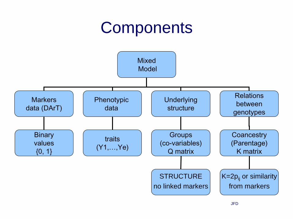
Components

Mixed

Model

Markers

data (DArT)

Phenotypic

data

Underlying

structure

Relations

between

genotypes

Binary

values

{0, 1}

traits

(Y1,…,Ye)

Groups

(co-variables)

Q matrix

Coancestry

(Parentage)

K matrix

STRUCTURE

no linked markers

K=2pij or similarity

from markers

JFD

geno y2 gr1 gr2 gr3 gr4 gr5 gr6 gr7 m45 m46 m47 m48

1 8.6 0.001 0.994 0.001 0.001 0.001 0.001 0.001 0 1 1 1

2 12.9 0.996 0.001 0.001 0.001 0.000 0.000 0.001 1 1 1 1

3 11.8 0.001 0.001 0.001 0.001 0.001 0.993 0.002 1 0 1 1

4 12.3 0.281 0.003 0.001 0.002 0.462 0.199 0.052 1 1 0 0

5 10.0 0.002 0.007 0.003 0.239 0.136 0.610 0.005 1 0 1 1

. . . . . . . . . . . . .

45 10.8 0.001 0.001 0.991 0.002 0.001 0.002 0.002 0 1 1 1

46 7.0 0.001 0.002 0.948 0.042 0.004 0.001 0.002 0 1 1 1

Data set (subset)(one environment, 7groups, 4 markers)

JFD

Proposition

• The marker is associated to the phenotype if the trait average for genotypes owning a “0” is “very”different to the trait average for genotypes owning a “1”

• “very”= statistically different in a test of hypothesis

• 3 possible models: one way anova, Q model, Q+K model

JFD

Q+K model (one site)

εZuXβ

ij

g

l ij

l

ij

l

iij qy1

1 )(

)()( ˆ

fixed random

i = 1,2 (two states of marker)

i = 1 if the ith marker is present in jth genotype

= membership probability of the jth genotype to the lth group

j(i) = genotype nested in the marker state (i=1 or i=0)

)(ˆ l

ijq

JFD

Variance-covariance matrices

2

2

)(

)(

aAuV

V Iε

• A is known: coefficient of parentage or some similarity using non linked markers

• Variances should be estimated

JFD

matrix K (= A)

JFD

Bonferroni bound

(when tests are not independent)

• Example: m=46 tests, =0.05,

P[reject at least one Ho/Ho true] =

1-(1- )m = = 1-(0.95)46 = 0.906

• if you want 0.05 “on all tests” type I error

Reject Ho when

001114.0)05.01(1ˆ 461

JFD

Results (yield)

(10 environments, 374 DArT, Q+K model)

0.10 0.05

Site DART F p p<=0.00028 p<=0.000138

348 wPt-0086 14.9740 1.26E-04 1 1

275 wPt-1859 14.3168 1.77E-04 1 0

279 wPt-3992 15.1771 1.13E-04 1 1

194 wPt-4115 15.3556 1.04E-04 1 1

163 wPt-4487 24.1353 1.27E-06 1 1

234 wPt-9075 19.5032 1.30E-05 1 1

424 wPt-9930 14.7447 1.42E-04 1 0

total 7 5

JFD

Methodological Research

1. The Ward-MLM three-way strategy for classifying genetic resources in multiple environments

2. Sampling strategies for conserving diversity when forming core subsets using genetic markers

JFD

Interdisciplinary group

• Jose Crossa CIMMYT-Biometrics

• Suketoshi Taba CIMMYT-Maize Genebank

• Marilyn Warburton CIMMYT-USDA-Molecular

genetics

• Sarah Hearne IITA- Molecular genetics

• Steve A. Eberhart USDA-Genebank

• Jose Villaseñor C. P.-mathematics

• Jorge Franco UDELAR-CIMMYT-Biometrics

JFD

The Ward-MLM three-way strategy

for classifying genetic resources in

multiple environments: evaluate GxE

Franco et al (2003) Crop Sci 43; 1249-1258

JFD

Properties of the Ward-MLM strategy

1. It assigns the observations to an optimal number of

clusters based on membership probability (is a

statistical method)

2. It uses discrete an continuous variables simultaneously

3. It follows the optimization of two objective functions

(minimum variance within group, and maximum Log-

likelihood)

4. It allows the estimation of the quality of the resulting

clustering (average of the assignment probabilities)

5. It can be used on 3-way data sets (genotype ×

environment × trait).

JFD

Example256 Caribbean maize genotypes

Discrete variable :

• Agronomic Scale (1=poor, 2=regular, 3=good)

Continuous variables:

• Days to anthesis (DA)

• Plant height (PH, cm)

• Days to senescence of the ear leave (DS)

• Ear length (EL, cm)

Three environments (Mexico)

JFD

Information to the 3-way analysis

(first 5 observations)

NOBS DA1 PH1 DS1 EL1 DA2 PH2 DS2 EL2 DA3 PH3 DS3 EL3 AS1 AS2 AS3

1 73.5 222.4 45.5 14.7 91.6 210.0 48.1 17.3 59.8 262.8 45.8 21.0 1 2 3

2 71.4 225.7 47.5 14.9 90.1 209.8 40.0 13.1 61.7 262.3 43.9 15.5 2 2 2

3 64.5 165.8 51.1 13.5 75.6 171.3 56.5 16.4 54.3 224.1 47.4 17.5 2 3 2

4 73.5 180.3 47.5 12.2 91.9 176.2 49.7 16.3 61.1 234.8 55.0 17.5 2 2 3

5 74.5 200.5 50.4 15.3 93.0 186.6 56.8 16.2 61.2 249.1 51.4 19.0 3 3 3

JFD

Canonical representation (87%)

-8

-6

-4

-2

0

2

4

6

-10 -8 -6 -4 -2 0 2 4 6 8 10

Can 1 (DS+, DA-, EL+,79%)

Ca

n 2

(E

L+

,PH

+, 8

%)

G1

G2

G3

G4

G5

G6

G7

G8

JFD

Agronomic performance of genotypes

Group good(GGG,GGR)

Regular Poor(RPP,PPP)

Non id.(GRP)

1 (46) 46

2 (25) 18 5 2

3 (27) 19 8

4 (53) 53

5 (24) 24

6 (22) 13 9

7 (32) 7 19 6

8 (27) 3 24

JFD

Average values groups 5 and 8

DA PH DS EL AgS

G E1 E2 E3 E1 E2 E3 E1 E2 E3 E1 E2 E3 E1 E2 E3 n

5 75 94 63 213 218 266 45 52 49 15 16 19 3.0 3.0 2.9 24

8 81 102 70 218 219 257 38 43 39 13 15 16 1.3 1.4 1.0 27

m 77 97 66 214 218 266 42 48 45 14 16 18 1.9 2.0 2.4 256

JFD

group X environment interaction

(no COI)

50

60

70

80

90

100

110

0 1 2 3 4 5 6 7 8 9

group

env 1

env 2

env 3

190

200

210

220

230

240

250

260

270

280

0 1 2 3 4 5 6 7 8 9

group

env 1

env 2

env 3

35

40

45

50

55

0 1 2 3 4 5 6 7 8 9

group

env 1

env 2

env 3

12

13

14

15

16

17

18

19

20

0 1 2 3 4 5 6 7 8 9

group

env 1

env 2

env 3

DA

DS EL

PH

JFD

Agronomic scale (COI**)

0.5

1.0

1.5

2.0

2.5

3.0

3.5

0 1 2 3 4 5 6 7 8 9

group

env 1

env 2

env 3

JFD

Variable relations vs Environment

(between groups)

-0.8

-0.6

-0.4

-0.2

0.0

0.2

0.4

0.6

0.8

-1.0 -0.5 0.0 0.5 1.0 1.5

Dimension 1

Dim

en

sio

n 2 Env 1

env 2

env 3

QDS1

EL1

PH1

DA1

EL2

PH2

EL3

PH3

DA2

DA3

DS3

DS2

Q2

Q3

Q1

-0.17

0.29

0.53

-0.94

-0.88

-0.87

JFD

• DEF: A core collection (or core subset) is a

sample from a large germplasm collection that

contains, with a minimum of repetitiveness, the

maximum possible genetic diversity of the

species in question (Frankel and Brown, 1984)

• Forming core subsets requires sampling

Sampling strategies for conserving diversity

when forming core subsets using genetic

markers

JFD

STEP 1. Numerical classification

• The most used methods are Ward (minimumvariance within cluster), and UPGMA (average ofdistances)

• They require an initial matrix of distances betweengenotypes

• With SSR we can use genetic distances (ModifiedRogers, Cavalli-Sforza & Edwards). Both are Euclidianmetrics

JFD

STEP 2. drawing accessions from clusters

(how many accessions from each cluster?)

Allocation methods : are methods for determining the number of observations to be randomly drawn from each stratum (cluster)

Optimal (Neyman): proportional to the size and variability of the cluster

P: proportional to the cluster size

L: proportional to the log of the cluster size

JFD

t t

ii

d

dnn

ni: number of accessions to be drawn from ith cluster

di: average of distances between accessions withinthe ith cluster

n: size of the core subset

t = 1,2,…,number of clusters

D-method: proportional to any measure of the

cluster diversity

Franco et al (2006) Crop Sci 46; 854-864

JFD

Diversity

Diversity indexes

(allele richness)

Expected

heterozygosis

(He)

Number of

effective alleles

(Ne)

Shannon Index

Distances among

Individuals

or groups

Non informative

Markers

p {0,1}

Informative

Markers

p [0,1]

Modified RogersSimple Matching

Jaccard

Nei and Li

(Dice)

Cavalli-Sforza and

Edwards

Euclidian

JFD

Example: three maize data sets

(SSR markers)

Obs. Alleles Markers Values Missing

Bulks 275 186 24 [0, 1] 1.5 %

Landraces 521 209 26 {0,.5,1} no

Populations 25 209 26 [0, 1] no

JFD

24 stratified strategies + MSTRAT

(20 independent core subsets)

Code Cluster Distance Allocation methods

1

to

12

Ward

Modified

Rogers

P, L,

D: MR,SH,HE,NE

Cavalli-S &

Edwards

P, L,

D: CE,SH,HE,NE

13

To

24

Average

(UPGMA)

Modified

Rogers

P, L,

D: MR,SH,HE,NE

Cavalli-S &

Edwards

P, L,

D: CE,SH,HE,NE

25 MSTRAT (non stratified method)

JFD

Bulk data set

MRs

CEs

SHs

HEs

NEs

Best strategy (24)† 0.503a 0.578a 4.411b 0.626b 2.980b

M-Strategy 0.467b 0.559b 4.478a 0.644a 3.166a

Entire collection 0.440 0.521 4.399 0.620 2.937

δ'(%) 1.37 1.20 0.31 0.77 1.60

Landraces data set

MRs

CEs

SHs

HEs

NEs

Best strategy (24) 0.653a 0.719a 4.525a 0.619a 2.963a

M-Strategy 0.637b 0.704b 4.504b 0.599b 2.808b

Entire collection 0.635 0.700 4.467 0.591 2.742

δ'(%) 0.48 0.37 0.26 0.82 1.23

Means of 20 reps (different core subsets)

† (24) UPGMA – Cavalli-sforza & Edwards – Number of effective alleles

JFD

Bulks

-4

-3

-2

-1

0

1

2

3

-4 -3 -2 -1 0 1 2 3 4

Dim-1

Dim

-2

Data U-CE-NE (24) MSTRAT

JFD

Landraces

-3

-2

-1

0

1

2

3

-3 -2 -2 -1 -1 0 1 1 2 2 3

Dim-1

Dim

-2

Data U-CE-NE (24) MSTRAT

JFD

Conclusions

• When constructing core subsets of individuals(landraces/accessions) the D allocation method usedwith a stratified sampling strategy was better than the Mstrategy

• For bulks and populations the M-strategy was better fordiversity indexes.

• Some stratified sampling strategies (21-24) were alwaysbetter showing the higher average distance (MR, andCE) between accessions

• All 25 strategies selected non-informative alleles but theM strategy selected less than the others.

JFD

Uses of D allocation method

• D method was used define reference

collections for inbred lines and populations

of maize from Mexico with Marilyn

Warburton from CIMMYT

• D method was used in a collaboration with

Sarah Hearne of IITA to define the

reference germplasm collection of cowpea

accessions

JFD

Current research

A method for classifying genotypes

using phenotypic and genotypic

information simultaneously

Phenotypic: continuous and categorical

Genotypic: SSR, DART, SNP

We have a draft