Embed Size (px)
Citation preview

The Art of Querying – Newest and Advanced SQL Techniques
Zohar Elkayam CTO, Brillix
Twitter: @realmgic

2
• Zohar Elkayam, CTO at Brillix
• Programmer, DBA, team leader, database trainer, public speaker, and a senior consultant for over 19 years
• Oracle ACE Since 2014
• ilOUG Board Member – Israel Oracle User Group
• Blogger – www.realdbamagic.com and www.ilDBA.co.il
Who am I?

3
About Brillix
• We offer complete, integrated end-to-end solutions based on best-of-breed innovations in database, security and big data technologies
• We provide complete end-to-end 24x7 expert remote database services
• We offer professional customized on-site trainings, delivered by our top-notch world recognized instructors

4
Some of Our Customers

5
• Founded in 1999, over 7000 members at its peak
• Divided into Technologies (Databases) and Applications groups
• Free Bi-monthly meetups for DBAs and Developers at Oracle Israel offices
• Yearly conference with guests speakers from all over the world:• January 22-23, 2018• Over 30 Speakers from all over the world: Ask TOM team, Oracle product mangers
and Oracle ACEs from 9 different countries!
• You can join our community: meetup group, facebook group or follow us on twitter (@ilOUG_org)!
• Our website: www.ilOUG.org
ilOUG – Israel Oracle User Group

6
Agenda
• Aggregative and advanced grouping options
• Analytic functions, ranking and pagination
• Hierarchical and recursive queries
• Regular Expressions
• Oracle 12c new rows pattern matching
• XML and JSON handling with SQL
• Oracle 12c (12.1 + 12.2) new features
• SQL Developer Command Line tool (if time allows)

7
Our Goal Today
• Learning new SQL techniques
• We will not expert everything
• Getting to know new features (12cR1 and 12cR2)
• Did you hear about Oracle 18c?
• This is a starting point – don’t be afraid to try

8
.בסיום יום הסמינר יחולק טופס משוב ונשמח לקבל את חוות דעתכם•
!היא זו המאפשרת לנו לעשות את הסמינרים טובים יותר:דעתכם חשובה•
Our REAL Agenda
הפסקה10:30-10:45
י הכנס בגן המלוןארוחת צהריים לכל משתתפ12:30-13:30
הפסקה מתוקה במתחם קבלת הפנים15:00-15:15
הולכים הביתה16:30

9
יכולות מתקדמות–Oracle SQLאודות
מדריך , יכולות מתקדמות–Oracle SQL"הספר •2011פורסם בשנת " לשולף המהיר
הראשון והיחיד שנכתב בעברית SQL-זה ספר ה•מתחילתו ועד סופו
הספר נכתב על ידי עמיאל דיוויס ועבר עריכה •טכנית שלי

10
SQL טכניקות ויישומים פרקטיים–מתקדם
טכניקות ויישומים –מתקדם SQL"הספר •הוא ספר שפורסם על ידי רם קדם" פרקטיים
(בעברית ובאנגלית)
מורכבות ופתרונןSQLבעיות 100-הספר מכיל כ•
קיים גם בגרסת אונליין•
/http://ramkedem.com: לפרטים•

11
Oracle LiveSQL
• Oracle provides free "live" 12.2 SQL tool• Includes available code library
• Ability to save scripts and share
• Online database design including Sample Schemas
• Some features don’t work as expected (example, later)
• https://livesql.oracle.com
• A short demo before we start…
12
ANSI SQL
• SQL was invented in 1970 by Dr. E. F. Codd
• Each vendor had its own flavor of SQL
• Standardized by ANSI since 1986
• Current stable standard is ANSI SQL:2011/2008
• Oracle 11g is compliant to SQL:2008
• Oracle 12c is fully compliant to CORE SQL:2011

13
Queries
• In this seminar we will only talk about queries

Group FunctionsMore than just group by…

15
Group Function and SQL
• Using SQL for aggregation:• Group functions basics
• The CUBE and ROLLUP extensions to the GROUP BY clause
• The GROUPING functions
• The GROUPING SETS expression
• Working with composite columns
• Using concatenated groupings

16
Basics
• Group functions will return a single row for each group
• The group by clause groups rows together and allows group functions to be applied
• Common group functions: SUM, MIN, MAX, AVG, etc.

17
Group Functions Syntax
SELECT [column,] group_function(column). . .
FROM table
[WHERE condition]
[GROUP BY group_by_expression]
[ORDER BY column];
SELECT AVG(salary), STDDEV(salary),
COUNT(commission_pct),MAX(hire_date)
FROM hr.employees
WHERE job_id LIKE 'SA%';

18
SELECT department_id, job_id, SUM(salary),
COUNT(employee_id)
FROM hr.employees
GROUP BY department_id, job_id
Order by department_id;
The GROUP BY Clause
SELECT [column,] group_function(column)
FROM table
[WHERE condition]
[GROUP BY group_by_expression]
[ORDER BY column];

19
The HAVING Clause
• Use the HAVING clause to specify which groups are to be displayed
• You further restrict the groups on the basis of a limiting condition
SELECT [column,] group_function(column)...
FROM table
[WHERE condition]
[GROUP BY group_by_expression]
[HAVING having_expression]
[ORDER BY column];

20
GROUP BY Using ROLLUP and CUBE
• Use ROLLUP or CUBE with GROUP BY to produce superaggregate rows by cross-referencing columns
• ROLLUP grouping produces a result set containing the regular grouped rows and the subtotal and grand total values
• CUBE grouping produces a result set containing the rows from ROLLUP and cross-tabulation rows
21
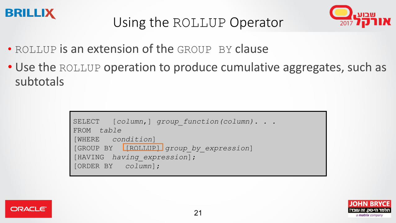
Using the ROLLUP Operator
• ROLLUP is an extension of the GROUP BY clause
• Use the ROLLUP operation to produce cumulative aggregates, such as subtotals
SELECT [column,] group_function(column). . .
FROM table
[WHERE condition]
[GROUP BY [ROLLUP] group_by_expression]
[HAVING having_expression];
[ORDER BY column];

22
Using the ROLLUP Operator: Example
SELECT department_id, job_id, SUM(salary)
FROM hr.employees
WHERE department_id < 60
GROUP BY ROLLUP(department_id, job_id);
1
2
3
Total by DEPARTMENT_ID
and JOB_ID
Total by DEPARTMENT_ID
Grand total

23
Using the CUBE Operator
• CUBE is an extension of the GROUP BY clause
• You can use the CUBE operator to produce cross-tabulation values with a single SELECT statement
SELECT [column,] group_function(column)...
FROM table
[WHERE condition]
[GROUP BY [CUBE] group_by_expression]
[HAVING having_expression]
[ORDER BY column];

24
SELECT department_id, job_id, SUM(salary)
FROM hr.employees
WHERE department_id < 60
GROUP BY CUBE (department_id, job_id);
. . .
Using the CUBE Operator: Example
. . .
1
2
3
4
Grand total
Total by JOB_ID
Total by DEPARTMENT_ID
and JOB_ID
Total by DEPARTMENT_ID
25
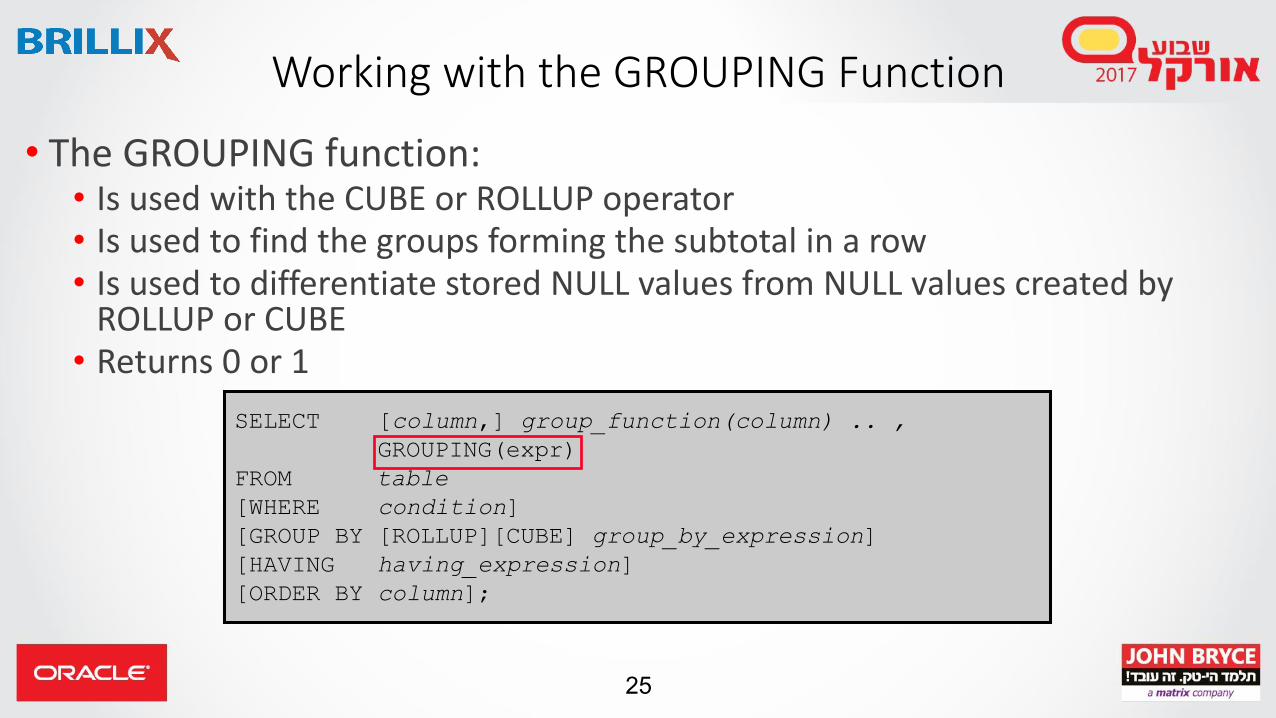
SELECT [column,] group_function(column) .. ,
GROUPING(expr)
FROM table
[WHERE condition]
[GROUP BY [ROLLUP][CUBE] group_by_expression]
[HAVING having_expression]
[ORDER BY column];
Working with the GROUPING Function
• The GROUPING function: • Is used with the CUBE or ROLLUP operator• Is used to find the groups forming the subtotal in a row• Is used to differentiate stored NULL values from NULL values created by
ROLLUP or CUBE• Returns 0 or 1
26
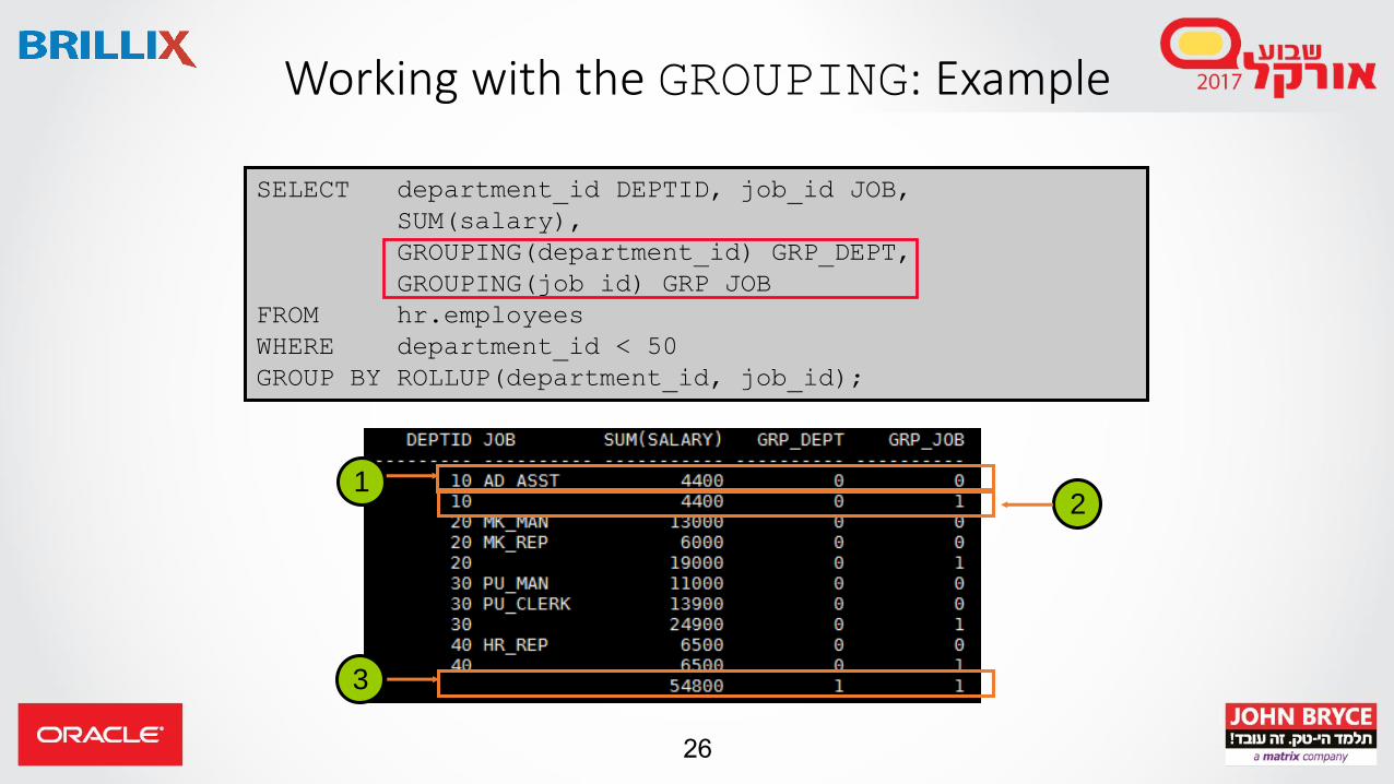
SELECT department_id DEPTID, job_id JOB,
SUM(salary),
GROUPING(department_id) GRP_DEPT,
GROUPING(job_id) GRP_JOB
FROM hr.employees
WHERE department_id < 50
GROUP BY ROLLUP(department_id, job_id);
Working with the GROUPING: Example
12
3

27
Working with GROUPING_ID Function
• Extension to the GROUPING function
• GROUPING_ID returns a number corresponding to the GROUPING bit vector associated with a row
• Useful for understanding what level the row is aggregated at and filtering those rows

28
GROUPING_ID Function ExampleSELECT department_id DEPTID, job_id JOB,
SUM(salary),
GROUPING_ID(department_id,job_id) GRP_ID
FROM hr.employees
WHERE department_id < 40
GROUP BY CUBE(department_id, job_id);
DEPTID JOB SUM(SALARY) GRP_ID
---------- ---------- ----------- ----------
48300 3
MK_MAN 13000 2
MK_REP 6000 2
PU_MAN 11000 2
AD_ASST 4400 2
PU_CLERK 13900 2
10 4400 1
10 AD_ASST 4400 0
20 19000 1
20 MK_MAN 13000 0
20 MK_REP 6000 0
30 24900 1
30 PU_MAN 11000 0
30 PU_CLERK 13900 0

29
Working with GROUP_ID Function
• GROUP_ID distinguishes duplicate groups resulting from a GROUPBY specification
• A Unique group will be assigned 0, the non unique will be assigned 1 to n-1 for n duplicate groups
• Useful in filtering out duplicate groupings from the query result

30
GROUP_ID Function Example
SELECT department_id DEPTID, job_id JOB,
SUM(salary),
GROUP_ID() UNIQ_GRP_ID
FROM hr.employees
WHERE department_id < 40
GROUP BY department_id, CUBE(department_id, job_id);
DEPTID JOB SUM(SALARY) UNIQ_GRP_ID
---------- ---------- ----------- -----------
10 AD_ASST 4400 0
20 MK_MAN 13000 0
20 MK_REP 6000 0
30 PU_MAN 11000 0
30 PU_CLERK 13900 0
10 AD_ASST 4400 1
20 MK_MAN 13000 1
20 MK_REP 6000 1
30 PU_MAN 11000 1
30 PU_CLERK 13900 1
10 4400 0
20 19000 0
30 24900 0
10 4400 1
20 19000 1
30 24900 1

31
GROUPING SETS
• The GROUPING SETS syntax is used to define multiple groupings in the same query.
• All groupings specified in the GROUPING SETS clause are computed and the results of individual groupings are combined with a UNIONALL operation.
• Grouping set efficiency:• Only one pass over the base table is required.• There is no need to write complex UNION statements.• The more elements GROUPING SETS has, the greater the performance
benefit.

33
SELECT department_id, job_id,
manager_id, AVG(salary)
FROM hr.employees
GROUP BY GROUPING SETS
((department_id,job_id), (job_id,manager_id));
GROUPING SETS: Example
. . .
1
2

35
Composite Columns
• A composite column is a collection of columns that are treated as a unit.ROLLUP (a,(b,c), d)
• Use parentheses within the GROUP BY clause to group columns, so that they are treated as a unit while computing ROLLUP or CUBEoperators.
• When used with ROLLUP or CUBE, composite columns require skipping aggregation across certain levels.

37
SELECT department_id, job_id, manager_id,
SUM(salary)
FROM hr.employees
GROUP BY ROLLUP( department_id,(job_id, manager_id));
Composite Columns: Example
1
2
3
4

39
Concatenated Groupings
• Concatenated groupings offer a concise way to generate useful combinations of groupings.
• To specify concatenated grouping sets, you separate multiple grouping sets, ROLLUP, and CUBE operations with commas so that the Oracle server combines them into a single GROUP BY clause.
• The result is a cross-product of groupings from each GROUPING SET.
GROUP BY GROUPING SETS(a, b), GROUPING SETS(c, d)

40
SELECT department_id, job_id, manager_id,
SUM(salary)
FROM hr.employees
GROUP BY department_id,
ROLLUP(job_id),
CUBE(manager_id);
Concatenated Groupings: Example
…
…
…
1
3
4
5
6
2
7
…
…

Analytic FunctionsLet’s analyze our data!

42
Overview of SQL for Analysis and Reporting
• Oracle has enhanced SQL's analytical processing capabilities by introducing a new family of analytic SQL functions.
• These analytic functions enable you to calculate and perform:• Rankings and percentiles
• Pivoting operations
• Moving window calculations
• LAG/LEAD analysis
• FIRST/LAST analysis
• Linear regression statistics

43
Why Use Analytic Functions?
• Ability to see one row from another row in the results
• Avoid self-join queries
• Summary data in detail rows
• Slice and dice within the results

44
Using the Analytic Functions
Function type Used for
Ranking Calculating ranks, percentiles, and n-tiles of the values in a
result set
Windowing Calculating cumulative and moving aggregates, works with functions such as SUM, AVG, MIN, and so on
Reporting Calculating shares such as market share, works with functions such as SUM, AVG, MIN, MAX, COUNT, VARIANCE,
STDDEV, RATIO_TO_REPORT, and so on
LAG/LEAD Finding a value in a row or a specified number of rows
from a current row
FIRST/LAST First or last value in an ordered group
Linear Regression Calculating linear regression and other statistics

45
Concepts Used in Analytic Functions
• Result set partitions: These are created and available to any aggregate results such as sums and averages. The term “partitions” is unrelated to the table partitions feature.
• Window: For each row in a partition, you can define a sliding window of data, which determines the range of rows used to perform the calculations for the current row.
• Current row: Each calculation performed with an analytic function is based on a current row within a partition. It serves as the reference point determining the start and end of the window.

47
Reporting Functions
• We can use aggregative/group functions as analytic functions (i.e. SUM, AVG, MIN, MAX, COUNT etc.)
• Each row will get the aggregative value for a given partition without the need for group by clause so we can have multiple group by’s on the same row
• Getting the raw data along with the aggregated value
• Use Order By to get cumulative aggregations

48
Reporting Functions Examples
SELECT last_name, salary, department_id,
ROUND(AVG(salary) OVER (PARTITION BY department_id),2),
COUNT(*) OVER (PARTITION BY manager_id),
SUM(salary) OVER (PARTITION BY department_id ORDER BY salary),
MAX(salary) OVER ()
FROM hr.employees;

Ranking Functions

50
Using the Ranking Functions
• A ranking function computes the rank of a record compared to other records in the data set based on the values of a set of measures. The types of ranking function are:
• RANK and DENSE_RANK functions
• PERCENT_RANK function
• ROW_NUMBER function
• NTILE function
• CUME_DIST function

51
Working with the RANK Function
• The RANK function calculates the rank of a value in a group of values, which is useful for top-N and bottom-N reporting.
• For example, you can use the RANK function to find the top ten products sold in Boston last year.
• When using the RANK function, ascending is the default sort order, which you can change to descending.
• Rows with equal values for the ranking criteria receive the same rank. • Oracle Database then adds the number of tied rows to the tied rank to
calculate the next rank.
RANK ( ) OVER ( [query_partition_clause] order_by_clause )

52
Using the RANK Function: Example
SELECT department_id, last_name, salary,
RANK() OVER (PARTITION BY department_id
ORDER BY salary DESC) "Rank"
FROM employees
WHERE department_id = 60
ORDER BY department_id, "Rank", salary;

53
Per-Group Ranking
• The RANK function can be made to operate within groups - that is, the rank gets reset whenever the group changes
• This is accomplished with the PARTITION BY clause
• The group expressions in the PARTITION BY sub-clause divide the data set into groups within which RANK operates
• For example: to rank products within each channel by their dollar sales, you could issue a statement similar to the one in the next slide.

54
Per-Group Ranking: Example
SELECT channel_desc, calendar_month_desc, TO_CHAR(SUM(amount_sold),
'9,999,999,999') SALES$, RANK() OVER (PARTITION BY channel_desc
ORDER BY SUM(amount_sold) DESC) AS RANK_BY_CHANNEL
FROM sales, products, customers, times, channels
WHERE sales.prod_id = products.prod_id
AND sales.cust_id = customers.cust_id
AND sales.time_id = times.time_id
AND sales.channel_Id = channels.channel_id
AND times.calendar_month_desc IN ('2000-08', '2000-09', '2000-
10', '2000-11')
AND channels.channel_desc IN ('Direct Sales', 'Internet')
GROUP BY channel_desc, calendar_month_desc;

55
RANK and DENSE_RANK Functions: Example
SELECT department_id, last_name, salary,
RANK() OVER (PARTITION BY department_id
ORDER BY salary DESC) "Rank",
DENSE_RANK() over (partition by department_id
ORDER BY salary DESC) "Drank"
FROM employees
WHERE department_id = 60
ORDER BY department_id, last_name, salary DESC, "Rank"
DESC;
DENSE_RANK ( ) OVER ([query_partition_clause] order_by_clause)

56
Per-Cube and Rollup Group Ranking
SELECT channel_desc, country_iso_code,
TO_CHAR(SUM(amount_sold), '9,999,999,999')SALES$,
RANK() OVER
(PARTITION BY GROUPING_ID(channel_desc, country_iso_code)
ORDER BY SUM(amount_sold) DESC) AS RANK_PER_GROUP
FROM sales, customers, times, channels, countries
WHERE sales.time_id = times.time_id AND
sales.cust_id=customers.cust_id AND
sales.channel_id = channels.channel_id AND
channels.channel_desc IN ('Direct Sales', 'Internet') AND
times.calendar_month_desc='2000-09' AND
country_iso_code IN ('GB', 'US', 'JP')
GROUP BY CUBE(channel_desc, country_iso_code);

57
Using the PERCENT_RANK Function
• Uses rank values in its numerator and returns the percent rank of a value relative to a group of values
• PERCENT_RANK of a row is calculated as follows:
• The range of values returned by PERCENT_RANK is 0 to 1, inclusive. The first row in any set has a PERCENT_RANK of 0. The return value is NUMBER. Its syntax is:
(rank of row in its partition - 1) / (number of rows in
the partition - 1)
PERCENT_RANK () OVER ([query_partition_clause]
order_by_clause)

58
Using the PERCENT_RANK Function: Example
SELECT department_id, last_name, salary, PERCENT_RANK()
OVER (PARTITION BY department_id ORDER BY salary DESC)
AS pr
FROM hr.employees
ORDER BY department_id, pr, salary;

59
Working with the ROW_NUMBER Function
• The ROW_NUMBER function calculates a sequential number of a value in a group of values.
• When using the ROW_NUMBER function, ascending is the default sort order, which you can change to descending.
• Rows with equal values for the ranking criteria receive a different number.
ROW_NUMBER ( ) OVER ( [query_partition_clause] order_by_clause )

60
ROW_NUMBER VS. ROWNUM
• ROWNUM is a pseudo column, ROW_NUMBER is an actual function
• ROWNUM requires sorting of the entire dataset in order to return ordered list
• ROW_NUMBER will only sort the required rows thus giving better performance

61
Working With The NTILE Function
• Not really a ranking function
• Divides an ordered data set into a number of buckets indicated by expr and assigns the appropriate bucket number to each row
• The buckets are numbered 1 through expr
NTILE ( expr ) OVER ([query_partition_clause] order_by_clause)

62
Summary of Ranking Functions
• Different ranking functions may return different results if the data has ties
SELECT last_name, salary, department_id,
ROW_NUMBER() OVER (PARTITION BY department_id ORDER BY salary DESC) A,
RANK() OVER (PARTITION BY department_id ORDER BY salary DESC) B,
DENSE_RANK() OVER (PARTITION BY department_id ORDER BY salary DESC) C,
PERCENT_RANK() OVER (PARTITION BY department_id ORDER BY salary DESC) D,
NTILE(4) OVER (PARTITION BY department_id ORDER BY salary DESC) E
FROM hr.employees;

Inter-row Analytic Functions

64
Using the LAG and LEAD Analytic Functions
• LAG provides access to more than one row of a table at the same time without a self-join.
• Given a series of rows returned from a query and a position of the cursor, LAG provides access to a row at a given physical offset before that position.
• If you do not specify the offset, its default is 1.
• If the offset goes beyond the scope of the window, the optional defaultvalue is returned. If you do not specify the default, its value is NULL.
{LAG | LEAD}(value_expr [, offset ] [, default ])
OVER ([ query_partition_clause ] order_by_clause)
65
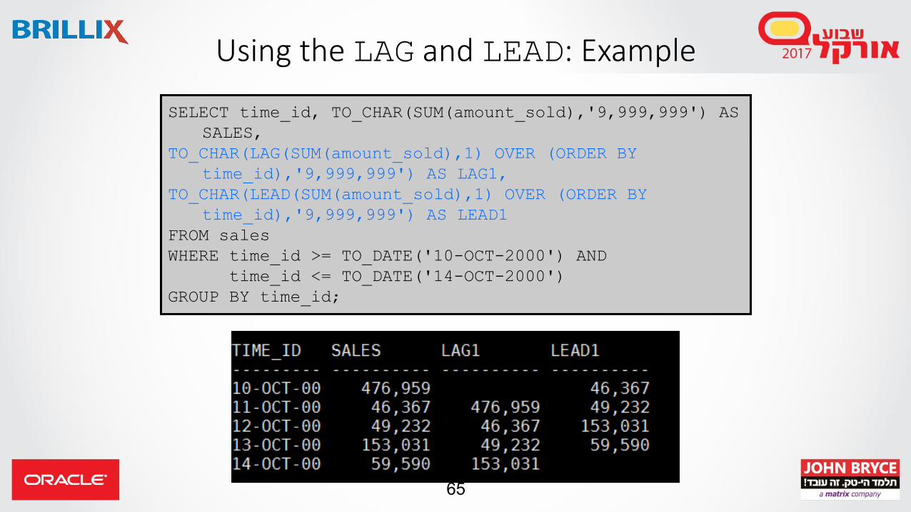
Using the LAG and LEAD: Example
SELECT time_id, TO_CHAR(SUM(amount_sold),'9,999,999') AS
SALES,
TO_CHAR(LAG(SUM(amount_sold),1) OVER (ORDER BY
time_id),'9,999,999') AS LAG1,
TO_CHAR(LEAD(SUM(amount_sold),1) OVER (ORDER BY
time_id),'9,999,999') AS LEAD1
FROM sales
WHERE time_id >= TO_DATE('10-OCT-2000') AND
time_id <= TO_DATE('14-OCT-2000')
GROUP BY time_id;

66
Using the LISTAGG Function
• For a specified measure, LISTAGG orders data within each group specified in the ORDER BY clause and then concatenates the valuesof the measure column
• Limited to 4000 chars (in 11g, see 12cR2 enhancement!)
LISTAGG(measure_expr [, 'delimiter'])
WITHIN GROUP (order_by_clause) [OVER
query_partition_clause]

67
Using LISTAGG: ExampleSELECT department_id "Dept", hire_date
"Date",
last_name "Name",
LISTAGG(last_name, ', ') WITHIN GROUP
(ORDER BY hire_date, last_name)
OVER (PARTITION BY department_id) as
"Emp_list"
FROM hr.employees
WHERE hire_date < '01-SEP-2003'
ORDER BY "Dept", "Date", "Name";
68
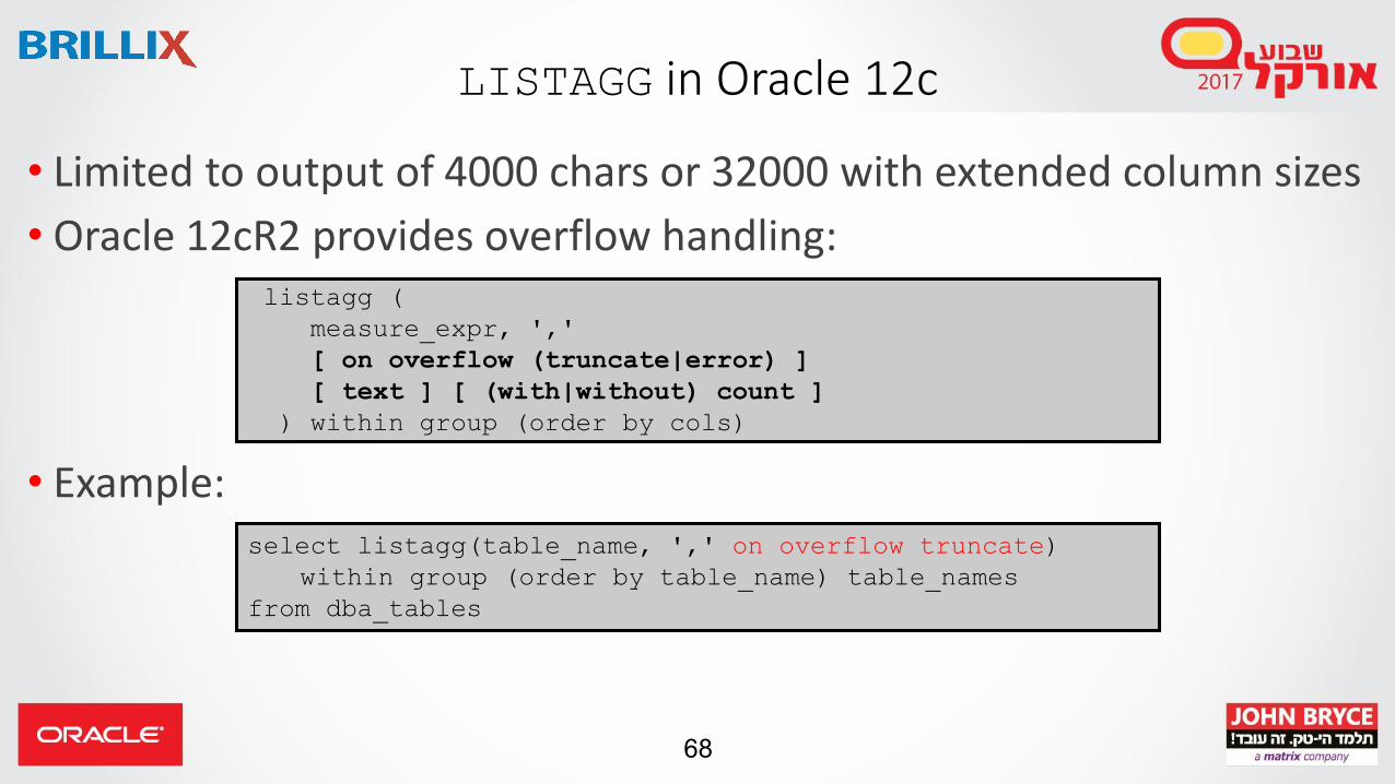
LISTAGG in Oracle 12c
• Limited to output of 4000 chars or 32000 with extended column sizes
• Oracle 12cR2 provides overflow handling:
• Example:
listagg (
measure_expr, ','
[ on overflow (truncate|error) ]
[ text ] [ (with|without) count ]
) within group (order by cols)
select listagg(table_name, ',' on overflow truncate)
within group (order by table_name) table_names
from dba_tables

69
Using the FIRST and LAST Functions
• Both are aggregate and analytic functions
• Used to retrieve a value from the first or last row of a sorted group, but the needed value is not the sort key
• FIRST and LAST functions eliminate the need for self-joins or views and enable better performance
aggregate_function KEEP
(DENSE_RANK FIRST ORDER BY
expr [ DESC | ASC ][ NULLS { FIRST | LAST } ]
[, expr [ DESC | ASC ] [ NULLS { FIRST | LAST } ]
]...
)
[ OVER query_partition_clause ]

70
FIRST and LAST Aggregate Example
SELECT department_id,
MIN(salary) KEEP (DENSE_RANK FIRST ORDER BY commission_pct)
"Worst",
MAX(salary) KEEP (DENSE_RANK LAST ORDER BY commission_pct)
"Best"
FROM employees
GROUP BY department_id
ORDER BY department_id;

71
FIRST and LAST Analytic Example
SELECT last_name, department_id, salary,
MIN(salary) KEEP (DENSE_RANK FIRST ORDER BY commission_pct)
OVER (PARTITION BY department_id) "Worst",
MAX(salary) KEEP (DENSE_RANK LAST ORDER BY commission_pct)
OVER (PARTITION BY department_id) "Best"
FROM employees
ORDER BY department_id, salary, last_name;

72
Using FIRST_VALUE/LAST_VALUEAnalytic Functions
• Returns the first/last value in an ordered set of values
• If the first value in the set is null, then the function returns NULL unless you specify IGNORE NULLS. This setting is useful for data densification
FIRST_VALUE (expr [ IGNORE NULLS ]) OVER (analytic_clause)
LAST_VALUE (expr [ IGNORE NULLS ]) OVER (analytic_clause)
73
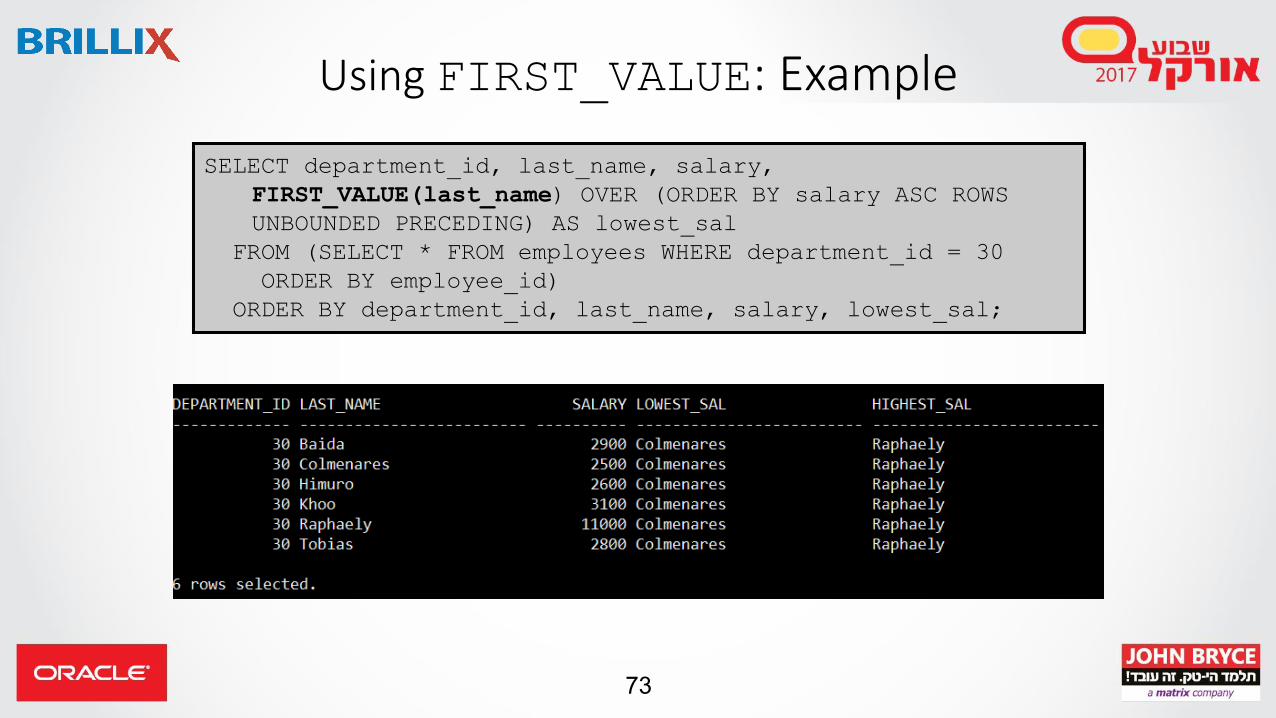
Using FIRST_VALUE: Example
SELECT department_id, last_name, salary,
FIRST_VALUE(last_name) OVER (ORDER BY salary ASC ROWS
UNBOUNDED PRECEDING) AS lowest_sal
FROM (SELECT * FROM employees WHERE department_id = 30
ORDER BY employee_id)
ORDER BY department_id, last_name, salary, lowest_sal;

74
Using NTH_VALUE Analytic Function
• Returns the N-th values in an ordered set of values
• Different default window: RANGE BETWEEN UNBOUNDED PRECEDING AND CURRENT ROW
NTH_VALUE (measure_expr, n)
[ FROM { FIRST | LAST } ][ { RESPECT | IGNORE } NULLS ]
OVER (analytic_clause)

75
Using NTH_VALUE: Example
SELECT prod_id, channel_id, MIN(amount_sold),
NTH_VALUE ( MIN(amount_sold), 2) OVER (PARTITION BY
prod_id ORDER BY channel_id
ROWS BETWEEN UNBOUNDED PRECEDING AND UNBOUNDED
FOLLOWING) nv
FROM sh.sales
WHERE prod_id BETWEEN 13 and 16
GROUP BY prod_id, channel_id;

76
Using NTH_VALUE: Example
SELECT prod_id, channel_id, MIN(amount_sold),
NTH_VALUE ( MIN(amount_sold), 2) OVER (PARTITION BY
prod_id ORDER BY channel_id
ROWS BETWEEN UNBOUNDED PRECEDING AND UNBOUNDED
FOLLOWING) nv
FROM sh.sales
WHERE prod_id BETWEEN 13 and 16
GROUP BY prod_id, channel_id;

Window Functions

78
Window Functions
• The windowing_clause gives some analytic functions a further degree of control over this window within the current partition
• The windowing_clause can only be used if an order_by_clause is present

79
Windows Can Be By RANGE Or ROWS
Possible values for start_point and end_point
UNBOUNDED PRECEDING The window starts at the first row of the partition. Only available for start points.
UNBOUNDED FOLLOWING The window ends at the last row of the partition. Only available for end points.
CURRENT ROW The window starts or ends at the current row
value_expr PRECEDING A physical or logical offset before the current row.When used with RANGE, can also be an interval literal
value_expr FOLLOWING As above, but an offset after the current row
RANGE BETWEEN start_point AND end_point
ROWS BETWEEN start_point AND end_point

80
Shortcuts
• Useful shortcuts for the windowing clause:
• The windows are limited to the current partition
• Generally, the default window is the entire work set unless said otherwise
ROWS UNBOUNDED PRECEDING ROWS BETWEEN UNBOUNDED PRECEDING AND CURRENT ROW
ROWS 10 PRECEDING ROWS BETWEEN 10 PRECEDING AND CURRENT ROW
ROWS CURRENT ROW ROWS BETWEEN CURRENT ROW AND CURRENT ROW

81
Windowing Clause Useful Usages
• Cumulative aggregation
• Sliding average over proceeding and/or following rows
• Using the RANGE parameter to filter aggregation records
Pivot and UnpivotTurning things around!

83
PIVOT and UNPIVOT
• You can use the PIVOT operator of the SELECT statement to write cross-tabulation queries that rotate the column values into new columns, aggregating data in the process.
• You can use the UNPIVOT operator of the SELECT statement to rotate columns into values of a column.
PIVOT UNPIVOT

84
Pivoting on the QUARTERColumn: Conceptual Example
30,000
40,000
60,000
30,000
40,000
20,000
AMOUNT_
SOLD
2,500Q1IUSAKids Jeans
2,000Q2CJapanKids Jeans
2,000Q3SUSAShorts
I
P
C
CHANNEL
Kids Jeans
Shorts
Shorts
PRODUCT
1,000Q2Germany
1,500Q4USA
Q2
QUARTER
2,500Poland
QUANTITY_
SOLD
COUNTRY
2,000
Q3
Kids Jeans
Shorts
PRODUCT
3,500
2,000
Q2
1,5002,500
Q4Q1

85
Pivoting Before Oracle 11g
• Pivoting the data before 11g was a complex query which required the use of the CASE or DECODE functions
select product,
sum(case when quarter = 'Q1' then amount_sold else null end) Q1,
sum(case when quarter = 'Q2' then amount_sold else null end) Q2,
sum(case when quarter = 'Q3' then amount_sold else null end) Q3,
sum(case when quarter = 'Q4' then amount_sold else null end) Q4
from sales
group by product;

86
PIVOT Clause Syntax
table_reference PIVOT [ XML ]
( aggregate_function ( expr ) [[AS] alias ]
[, aggregate_function ( expr ) [[AS] alias ] ]...
pivot_for_clause
pivot_in_clause )
-- Specify the column(s) to pivot whose values are to
-- be pivoted into columns.
pivot_for_clause =
FOR { column |( column [, column]... ) }
-- Specify the pivot column values from the columns you
-- specified in the pivot_for_clause.
pivot_in_clause =
IN ( { { { expr | ( expr [, expr]... ) } [ [ AS] alias] }...
| subquery | { ANY | ANY [, ANY]...} } )

88
Creating a New View: Example
CREATE OR REPLACE VIEW sales_view AS
SELECT
prod_name AS product,
country_name AS country,
channel_id AS channel,
SUBSTR(calendar_quarter_desc, 6,2) AS quarter,
SUM(amount_sold) AS amount_sold,
SUM(quantity_sold) AS quantity_sold
FROM sales, times, customers, countries, products
WHERE sales.time_id = times.time_id AND
sales.prod_id = products.prod_id AND
sales.cust_id = customers.cust_id AND
customers.country_id = countries.country_id
GROUP BY prod_name, country_name, channel_id,
SUBSTR(calendar_quarter_desc, 6, 2);

90
Selecting the SALES VIEW Data
SELECT product, country, channel, quarter, quantity_sold
FROM sales_view;
PRODUCT COUNTRY CHANNEL QUARTER QUANTITY_SOLD
------------ ------------ ---------- -------- -------------
Y Box Italy 4 01 21
Y Box Italy 4 02 17
Y Box Italy 4 03 20
. . .
Y Box Japan 2 01 35
Y Box Japan 2 02 39
Y Box Japan 2 03 36
Y Box Japan 2 04 46
Y Box Japan 3 01 65
. . .
Bounce Italy 2 01 34
Bounce Italy 2 02 43
. . .
9502 rows selected.

91
Pivoting the QUARTER Column in the SH Schema: Example
SELECT *
FROM
(SELECT product, quarter, quantity_sold
FROM sales_view) PIVOT (sum(quantity_sold)
FOR quarter IN ('01', '02', '03', '04'))
ORDER BY product DESC;
. . .

93
Unpivoting the QUARTER Column: Conceptual Example
2,000
Q3
Kids Jeans
Shorts
PRODUCT
3,500
2,000
Q2
1,5002,500
Q4Q1
2,500Q1Kids Jeans
2,000Q2Kids Jeans
3,500Q2Shorts
1,500Q4Kids Jeans
Q3
QUARTER
2,000Shorts
SUM_OF_QUANTITYPRODUCT

94
Unpivoting Before Oracle 11g
• Univoting the data before 11g requires multiple queries on the table using the UNION ALL operator
SELECT *
FROM (
SELECT product, '01' AS quarter, Q1_value FROM sales
UNION ALL
SELECT product, '02' AS quarter, Q2_value FROM sales
UNION ALL
SELECT product, '03' AS quarter, Q3_value FROM sales
UNION ALL
SELECT product, '04' AS quarter, Q4_value FROM sales
);

95
Using the UNPIVOT Operator
• An UNPIVOT operation does not reverse a PIVOT operation; instead, it rotates data found in multiple columns of a single row into multiple rows of a single column.
• If you are working with pivoted data, UNPIVOT cannot reverse any aggregations that have been made by PIVOT or any other means.
UNPIVOT

96
Using the UNPIVOT Clause
• The UNPIVOT clause rotates columns from a previously pivoted table or a regular table into rows. You specify:
• The measure column or columns to be unpivoted• The name or names for the columns that result from the UNPIVOT
operation
• The columns that are unpivoted back into values of the column specified in pivot_for_clause
• You can use an alias to map the column name to another value.

97
UNPIVOT Clause Syntax
table_reference UNPIVOT [{INCLUDE|EXCLUDE} NULLS]
-- specify the measure column(s) to be unpivoted.
( { column | ( column [, column]... ) }
unpivot_for_clause
unpivot_in_clause )
-- Specify one or more names for the columns that will
-- result from the unpivot operation.
unpivot_for_clause =
FOR { column | ( column [, column]... ) }
-- Specify the columns that will be unpivoted into values of
-- the column specified in the unpivot_for_clause.
unpivot_in_clause =
( { column | ( column [, column]... ) }
[ AS { constant | ( constant [, constant]... ) } ]
[, { column | ( column [, column]... ) }
[ AS { constant | ( constant [, constant]...) } ] ]...)

98
Creating a New Pivot Table: Example
. . .
CREATE TABLE pivotedtable AS
SELECT *
FROM
(SELECT product, quarter, quantity_sold
FROM sales_view) PIVOT (sum(quantity_sold)
FOR quarter IN ('01' AS Q1, '02' AS Q2,
'03' AS Q3, '04' AS Q4));
SELECT * FROM pivotedtable
ORDER BY product DESC;

99
Unpivoting the QUARTER Column : Example
• Unpivoting the QUARTER Column in the SH Schema:
SELECT *
FROM pivotedtable
UNPIVOT (quantity_sold For Quarter IN (Q1, Q2, Q3, Q4))
ORDER BY product DESC, quarter;
. . .
100
More Examples…
• More information and examples could be found on my Blog:
https://www.realdbamagic.com/he/pivot-a-table/

Top-N and Paging QueriesIn Oracle 12c

102
Top-N Queries
• A Top-N query is used to retrieve the top or bottom N rows from an ordered set
• Combining two Top-N queries gives you the ability to page through an ordered set
• Oracle 12c has introduced the row limiting clause to simplify Top-N queries

103
Top-N in 12cR1
• This is ANSI syntax
• The default offset is 0
• Null values in offset, rowcount or percent will return no rows
[ OFFSET offset { ROW | ROWS } ]
[ FETCH { FIRST | NEXT } [ { rowcount | percent PERCENT } ]
{ ROW | ROWS } { ONLY | WITH TIES } ]

104
Top-N Examples
SELECT last_name, salary
FROM hr.employees
ORDER BY salary
FETCH FIRST 4 ROWS ONLY;
SELECT last_name, salary
FROM hr.employees
ORDER BY salary
FETCH FIRST 4 ROWS WITH TIES;
SELECT last_name, salary
FROM hr.employees
ORDER BY salary DESC
FETCH FIRST 10 PERCENT ROWS ONLY;

105
Paging Before 12c
• Before 12c we had to use the rownum pseudo column to filter out rows
• That will require sorting the entire rowset
SELECT val
FROM (SELECT val, rownum AS rnum
FROM (SELECT val
FROM rownum_order_test
ORDER BY val)
WHERE rownum <= 10)
WHERE rnum >= 5;

106
Paging in Oracle 12c
• After 12c we have a syntax improvement for paging using the Top-N queries
• This will use ROW_NUMBER and RANK in the background – there is no real optimization improvements
SELECT val
FROM rownum_order_test
ORDER BY val
OFFSET 4 ROWS FETCH NEXT 5 ROWS ONLY;

107
More Examples
• More information and examples could be found on my blog:
https://www.realdbamagic.com/he/12c-top-n-query/

108
Analytic Functions and Performance
• Analytic functions has positive impact on performance for the most part
• Using analytic functions can reduce the number of table scans and reduce IO consumption
• The query might use more CPU and/or memory but it will usually run faster than the same result without analytic functions
• Top-N queries might struggle with cardinality evaluation when using the “With Ties” option

Common Table Expression and Subquery Factoring

110
Subquery Factoring
• The WITH clause, or subquery factoring clause, is part of the SQL-99 standard
• Introduced in Oracle 9.2
• The WITH produces a new inline view which we can query from
• Sometimes, the subquery is being cached (materialized) so it does not need to re-query the data again

111
Subquery Example
SELECT e.LAST_NAME AS employee_name,
dc.dept_count AS emp_dept_count
FROM employees e,
(SELECT DEPARTMENT_ID, COUNT(*) AS dept_count
FROM employees
GROUP BY DEPARTMENT_ID) dc
WHERE e.DEPARTMENT_ID = dc.DEPARTMENT_ID;
WITH dept_count AS (
SELECT DEPARTMENT_ID, COUNT(*) AS dept_count
FROM employees
GROUP BY DEPARTMENT_ID)
SELECT e.LAST_NAME AS employee_name,
dc.dept_count AS emp_dept_count
FROM employees e,
dept_count dc
WHERE e.DEPARTMENT_ID = dc.DEPARTMENT_ID;

112
Subquery Reuse
WITH dept_count AS (
SELECT DEPARTMENT_ID, COUNT(*) AS dept_count
FROM employees
GROUP BY DEPARTMENT_ID)
SELECT e1.LAST_NAME AS employee_name,
e2.LAST_NAME as Manager_name,
dc1.dept_count AS emp_dept_count,
dc2.dept_count as mgr_dept_count
FROM employees e1,
employees e2,
dept_count dc1,
dept_count dc2
WHERE e1.DEPARTMENT_ID = dc1.DEPARTMENT_ID and
e2.DEPARTMENT_ID = dc2.DEPARTMENT_ID and
e1.MANAGER_ID = e2.employee_id

113
Subquery Materialization
• In some cases, the with clause data might be automatically materialized into a global temporary table
• The data will be persistent for the query and will not have to be regenerated again and again
• We can force the database to materialize the view using /*+ materialize */
• We can also force the database to never materialize, by using the hint /*+ inline */

114
Functions in the WITH Clause (12.1)
• Oracle 12c allows us the definition of anonymous function within the scope of a query
with
function sumascii (str in varchar2) return number is
x number := 0;
begin
for i in 1..length (str)
loop
x := x + ascii (substr (str, i, 1)) ;
end loop;
return x;
end;
select /*+ WITH_PLSQL */ h.EMPLOYEE_ID, h.last_name,
sumascii (h.last_name)
from hr.employees h

Hierarchical Queries andRecursive Queries

116
Using Hierarchical Queries
• You can use hierarchical queries to retrieve data based on a natural hierarchical relationship between rows in a table.
• A relational database does not store records in a hierarchical way; therefore, a hierarchical query is possible only when a relationship exists between rows in a table.
• However, where a hierarchical relationship exists between the rows of a single table, a process called “tree walking” enables the hierarchy to be constructed.
• A hierarchical query is a method of reporting, with the branches of a tree in a specific order.

117
Business Challenges
• Getting all employees that report directly or indirectly to a manager
• Managing documents and folders
• Managing privileges
• Aggregating levels on the same row

118
Using Hierarchical Queries: Example
• Sample Data from the EMPLOYEES Table (HR schema)
• Kochhar, De Haan, and Hartstein report to the same manager (MANAGER_ID = 100)
• EMPLOYEE_ID = 100 is King
…

119
Natural Tree Structure
De Haan
HunoldWhalen
Kochhar
Higgins
Mourgos Zlotkey
Rajs Davies Matos
Gietz Ernst Lorentz
Hartstein
Fay
Abel Taylor Grant
Vargas
MANAGER_ID = 100 (Child)
EMPLOYEE_ID = 100 (Parent)
. . . . . .
. . .
. . .
. . .
King

120
Hierarchical Queries: Syntax
• Condition:
expr comparison_operator expr``
SELECT [LEVEL], column, expr...
FROM table
[WHERE condition(s)]
[START WITH condition(s)]
[CONNECT BY PRIOR condition(s)] ;

121
Walking the Tree: Specifying the Starting Point
• Use the START WITH clause to specify the starting point, that is, the row or rows to be used as the root of the tree:
• Specifies the condition that must be met• Accepts any condition that is valid in a WHERE clause
• For example, using the HR.EMPLOYEES table, start with the employee whose last name is Kochhar.
. . .
START WITH last_name = 'Kochhar'
START WITH column1 = value

122
Walking the Tree: Specifying the Direction
• The direction of the query is determined by the CONNECT BY PRIOR column placement.
• The PRIOR operator refers to the parent row.
CONNECT BY PRIOR column1 = column2
. . .
CONNECT BY PRIOR employee_id = manager_id
. . .
Parent key Child key

124
Specifying the Direction of the Query: From the Top Down
SELECT last_name||' reports to '||
PRIOR last_name "Walk Top Down"
FROM hr.employees
START WITH last_name = 'King'
CONNECT BY PRIOR employee_id = manager_id ;
. . .

125
Specifying the Direction of the Query: From the Bottom Up
SELECT employee_id, last_name, job_id, manager_id
FROM hr.employees
START WITH employee_id = 101
CONNECT BY PRIOR manager_id = employee_id ;

126
Using the LEVEL Pseudocolumn
Level 1root/
parent
Level 3parent/
child/leaf
Level 4leaf
De Haan
King
HunoldWhalen
Kochhar
Higgins
Mourgos Zlotkey
Rajs Davies Matos
Gietz Ernst Lorentz
Hartstein
Fay
Abel Taylor Grant
Vargas
Level 2parent/
child

127
Using the LEVEL Pseudo-column: Example
SELECT employee_id, last_name, manager_id, LEVEL
FROM hr.employees
START WITH employee_id = 100
CONNECT BY PRIOR employee_id = manager_id
ORDER siblings BY last_name;
. . .

128
Ordering the Tree
• Since regular ORDER BY rearrange the data by rows and messes the hierarchy order, we try to avoid using ORDER BY in a hierarchy query
• We can use the ORDER SIBLINGS BY clause to arrange the data for each level in the tree separately

129
Formatting Hierarchical Reports
• It is common to format Hierarchical reports using LEVEL and LPAD• Create a report displaying company management levels beginning with the
highest level and indenting each of the following levels.
SELECT LPAD(last_name, LENGTH(last_name)+
(LEVEL*2)-2,'_') AS org_chart
FROM hr.employees
START WITH first_name = 'Steven' AND last_name = 'King'
CONNECT BY PRIOR employee_id = manager_id
ORDER SIBLINGS BY last_name;

130
Result

131
Pruning Nodes and Branches
• Use the WHERE clause to eliminate a node
• Use the CONNECT BY clause to eliminate a branch
Kochhar
Higgins
Gietz
Whalen
Kochhar
HigginsWhalen
Gietz
. . .
WHERE last_name != 'Higgins'
. . .
CONNECT BY PRIOR employee_id = manager_id
AND last_name != 'Higgins'
1 2

132
Pruning Branches Example 1:Eliminating a Node
SELECT department_id, employee_id,last_name, job_id,
salary
FROM hr.employees
WHERE last_name != 'Higgins'
START WITH manager_id IS NULL
CONNECT BY PRIOR employee_id = manager_id;
. . .
. . .
. . .

133
Pruning Branches Example 2:Eliminating a Branch
SELECT department_id, employee_id,last_name, job_id,
salary
FROM hr.employees
START WITH manager_id IS NULL
CONNECT BY PRIOR employee_id = manager_id
AND last_name != 'Higgins';
. . .

134
Order of Precedence
• Join happens before connect by
• Where is happening after connect by
• Regular order by will rearrange the returning rows
• order siblings by will rearrange the returning rows for each level

135
Loops in Hierarchy Queries
• CONNECT_BY_ISCYCLE - pseudo column that returns 1 if the current row is a child which is also its ancestor (a row that cause loop), otherwise returns 0
• NOCYCLE – return rows from a query even if a loop exists in the data, without error. Part of the connect by clause

136
Other CONNECT BY Functionality
• CONNECT_BY_ISLEAF - pseudo column that returns 1 if the row doesn’t have any child records
• CONNECT_BY_ROOT – using this operator on a column, will return the value for that column from the root record
• SYS_CONNECT_BY_PATH – a function that returns the path from the root to the current row for a column (delimited by a chosen char)

137
Recursive Subquery Factoring
• ANSI SQL:2008 (Oracle 11g) introduced a new way to run hierarchical queries: Recursive Subquery Factoring using Subquery Factoring
• That will mean that a query will query itself using the WITH clause, making queries easier to write

138
Recursive Subquery Factoring Example
with mytree(id, parent_id, "level")
as
(
select id, parent_id, 1 as "level"
from temp_v
where id = 1
union all
select temp_v.id, temp_v.parent_id,
mytree."level" + 1
from temp_v, mytree
where temp_v.parent_id = mytree.id
)
Select * from mytree;
Stop Condition
Actual
Recursion

139
Warning: Performance
• Recursion and Hierarchies might have bad impact on performance
• Watch out for mega-trees – it has CPU and memory impacts
• Using recursion might lead for multiple IO reads of the same blocks

Regular Expression

141
Regular Expression
• Regular expression (regexp) is a sequence of characters that define a search pattern
• Commonly used for smart “Search and Replace” of patterns and for input validations of text
• Widely introduced in Oracle 10g (and it even existed even before that)

142
Common REGEXP Functions and Operators
REGEXP_LIKE Perform regular expression matching
REGEXP_REPLACE Extends the functionality of the REPLACEfunction by using patterns
REGEXP_SUBSTR Extends the functionality of the SUBSTRfunction by using patterns
REGEXP_COUNT Count the number of matches of the pattern in a given string
REGEXP_INSTR Extends the functionality of the INSTRfunction by using patterns

143
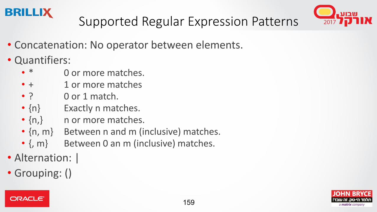
Supported Regular Expression Patterns
• Concatenation: No operator between elements.• Quantifiers:
• . Matches any character in the database character set• * 0 or more matches• + 1 or more matches• ? 0 or 1 match• {n} Exactly n matches• {n,} n or more matches• {n, m} Between n and m (inclusive) matches• {, m} Between 0 an m (inclusive) matches
• Alternation: [|]• Grouping: ()

144
Supported Regular Expression Patterns
Value Description
^Matches the beginning of a string. If used with a match_parameter of 'm', it matches the start of a line anywhere within expression.
$Matches the end of a string. If used with a match_parameter of 'm', it matches the end of a line anywhere withinexpression.
\W Matches a nonword character.
\s Matches a whitespace character.
\S matches a non-whitespace character.
\AMatches the beginning of a string or matches at the end of a string before a newline character.
\Z Matches at the end of a string.

145
Character Classes
Character Class Description
[:alnum:] Alphanumeric characters
[:alpha:] Alphabetic characters
[:blank:] Blank Space Characters
[:cntrl:] Control characters (nonprinting)
[:digit:] Numeric digits
[:graph:] Any [:punct:], [:upper:], [:lower:], and [:digit:] chars
[:lower:] Lowercase alphabetic characters
[:print:] Printable characters
[:punct:] Punctuation characters
[:space:]Space characters (nonprinting), such as carriage return, newline, vertical tab, and form feed
[:upper:] Uppercase alphabetic characters
[:xdigit:] Hexidecimal characters

Regular Expression Demo

147
Pitfalls
• Regular expressions might be slow when used on large amount of data
• Writing regular expression can be very tricky – make sure your pattern is correct
• Oracle REGEXP syntax is not standard, regular expression might not work or partially work causing wrong results
• There can only be up to 9 placeholders in a given quantifier

Pattern Matching inOracle 12c

149
What is Pattern Matching
• Identify and group rows with consecutive values
• Consecutive in this regards – row after row
• Uses regular expression like syntax to find patterns

150
Common Business Challenges
• Finding sequences of events in security applications
• Locating dropped calls in a CDR listing
• Financial price behaviors (V-shape, W-shape U-shape, etc.)
• Fraud detection and sensor data analysis

151
MATCH_RECOGNIZE Syntax
SELECT
FROM [row pattern input table]
MATCH_RECOGNIZE
( [ PARTITION BY <cols> ]
[ ORDER BY <cols> ]
[ MEASURES <cols> ]
[ ONE ROW PER MATCH | ALL ROWS PER MATCH ]
[ SKIP_TO_option]
PATTERN ( <row pattern> )
DEFINE <definition list>
)

152
Basix Syntax Legend
• PARTITION BY divides the data in to logical groups
• ORDER BY orders the data in each logical group
• MEASURES define the data measures of the pattern
• ONE/ALL ROW PER MATCH defines what to do with the pattern – return one row or all rows
• PATTERN says what the pattern actually is
• DEFINE gives us the condition that must be met for a row to map to the pattern variables

153
MATCH_RECOGNIZE Example
• Find Simple V-Shape with 1 row output per match
SELECT *
FROM Ticker MATCH_RECOGNIZE (
PARTITION BY symbol
ORDER BY tstamp
MEASURES STRT.tstamp AS start_tstamp,
LAST(DOWN.tstamp) AS bottom_tstamp,
LAST(UP.tstamp) AS end_tstamp
ONE ROW PER MATCH
AFTER MATCH SKIP TO LAST UP
PATTERN (STRT DOWN+ UP+)
DEFINE
DOWN AS DOWN.price < PREV(DOWN.price),
UP AS UP.price > PREV(UP.price)
) MR
ORDER BY MR.symbol, MR.start_tstamp;

154
What Will Be Matched?

155
Example: Sequential Employee IDs
• Our goal: find groups of users with sequences IDs
• This can be useful for detecting missing employees in a table, or to locate “gaps” in a group
FIRSTEMP LASTEMP
---------- ----------
7371 7498
7500 7520
7522 7565
7567 7653
7655 7697
7699 7781
7783 7787
7789 7838

156
Pattern Matching Example
SELECT *
FROM Emps
MATCH_RECOGNIZE (
ORDER BY emp_id
PATTERN (STRT B*)
DEFINE B AS emp_id = PREV(emp_id)+1
ONE ROW PER MATCH
MEASURES
STRT.emp_id firstemp,
LAST(emp_id) lastemp
AFTER MATCH SKIP PAST LAST ROW
);
1. Define input
2. Pattern Matching
3. Order input
4. Process pattern
5. Using defined conditions
6. Output: rows per match
7. Output: columns per row
8. Where to go after match?
Original concept by Stew Ashton

157
Pattern Matching Example
SELECT *
FROM Emps
MATCH_RECOGNIZE (
ORDER BY emp_id
MEASURES
STRT.emp_id firstemp,
LAST(emp_id) lastemp
ONE ROW PER MATCH
AFTER MATCH SKIP PAST LAST ROW
PATTERN (STRT B*)
DEFINE B AS emp_id = PREV(emp_id)+1
);
1. Define input
2. Pattern Matching
3. Order input
4. Process pattern
5. Using defined conditions
6. Output: rows per match
7. Output: columns per row
8. Where to go after match?
Original concept by Stew Ashton

158
Oracle 11g Analytic Function Solutionselect firstemp, lastemp
From (select nvl (lag (r) over (order by r), minr) firstemp, q
lastemp
from (select emp_id r,
lag (emp_id) over (order by emp_id) q,
min (emp_id) over () minr,
max (emp_id) over () maxr
from emps e1)
where r != q + 1 -- groups including lower end
union
select q,
nvl (lead (r) over (order by r), maxr)
from ( select emp_id r,
lead (emp_id) over (order by emp_id) q,
min (emp_id) over () minr,
max (emp_id) over () maxr
from emps e1)
where r + 1 != q -- groups including higher end
);
159
Supported Regular Expression Patterns
• Concatenation: No operator between elements.
• Quantifiers:• * 0 or more matches.• + 1 or more matches• ? 0 or 1 match.• {n} Exactly n matches.• {n,} n or more matches.• {n, m} Between n and m (inclusive) matches.• {, m} Between 0 an m (inclusive) matches.
• Alternation: |
• Grouping: ()

160
Functions
• CLASSIFIER(): Which pattern variable applies to which row
• MATCH_NUMBER(): Which rows are members of which match
• PREV(): Access to a column/expression in a previous row
• NEXT(): Access to a column/expression in the next row
• LAST(): Last value within the pattern match
• FIRST(): First value within the pattern match
• COUNT(), AVG(), MAX(), MIN(), SUM()

161
Example: All Rows Per Match
• Find suspicious transfers – a large transfer after 3 small ones
SELECT userid, match_id, pattern_variable, time, amount
FROM (SELECT * FROM event_log
WHERE event = 'transfer')
MATCH_RECOGNIZE
(
PARTITION BY userid ORDER BY time
MEASURES
MATCH_NUMBER() match_id,
CLASSIFIER() pattern_variable
ALL ROWS PER MATCH
PATTERN ( x{3,} y)
DEFINE
x AS (amount < 2000 AND LAST(x.time) -FIRST(x.time) < 30),
y AS (amount >= 1000000 AND y.time-LAST(x.time) < 10)
);

162
The Output
• MATCH_ID shows current match sequence
• PATTERN_VARIABLE show which variable was applied
• USERID is the partition key
USERID MATCH_ID PATTERN_VA TIME AMOUNT
-------- ---------- ---------- --------- ----------
john 1 X 06-JAN-12 1000
john 1 X 15-JAN-12 1500
john 1 X 20-JAN-12 1500
john 1 X 23-JAN-12 1000
john 1 Y 26-JAN-12 1000000

163
Example: One Row Per Match
• Same as before – show one row per match
SELECT userid, first_trx, last_trx, amount
FROM (SELECT * FROM event_log WHERE event = 'transfer')
MATCH_RECOGNIZE
(
PARTITION BY userid ORDER BY time
MEASURES
FIRST(x.time) first_trx,
y.time last_trx,
y.amount amount
ONE ROW PER MATCH
PATTERN ( x{3,} y )
DEFINE
x AS (amount < 2000 AND LAST(x.time) -FIRST(x.time) < 30),
y AS (amount >= 1000000 AND y.time-LAST(x.time) < 10)
);

164
The Output
• USERID is the partition key
• FIRST_TRX is a calculated measure
• AMOUNT and LAST_TRX are measures
USERID FIRST_TRX LAST_TRX AMOUNT
-------- --------- --------- ----------
john 06-JAN-12 26-JAN-12 1000000

165
Few Last Tips
• Test all cases: pattern matching can be very tricky
• Don’t forget to test your data with no matches
• There is no LISTAGG and no DISTINCT when using match recognition
• Pattern variables cannot be used as bind variables

Using XML with SQL
167
What is XML
• XML stand for eXtensible Markup Language
• Defines a set of rules for encoding documents in a format which is both human-readable and machine-readable
• Data is unstructured and can be transferred easily to other system

168
XML Terminology
• Root
• Element
• Attribute
• Forest
• XML Fragment
• XML Document

169
What Does XML Look Like?
<?xml version="1.0"?>
<ROWSET>
<ROW>
<USERNAME>SYS</USERNAME>
<USER_ID>0</USER_ID>
<CREATED>28-JAN-08</CREATED>
</ROW>
<ROW>
<USERNAME>SYSTEM</USERNAME>
<USER_ID>5</USER_ID>
<CREATED>28-JAN-08</CREATED>
</ROW>
</ROWSET>

170
Generating XML From Oracle
• Concatenating strings – building the XML manually. This is highly not recommended
• Using DBMS_XMLGEN
• Using ANSI SQL:2003 XML functions

171
Using DBMS_XMLGEN
• The DBMS_XMLGEN package converts the results of a SQL query to a canonical XML format
• The package takes an arbitrary SQL query as input, converts it to XML format, and returns the result as a CLOB
• Using the DBMS_XMLGEN we can create contexts and use it to build XML documents
• Old package – exists since Oracle 9i

172
Example of Using DBMS_XMLGEN
select dbms_xmlgen.getxml(q'{
select column_name, data_type
from all_tab_columns
where table_name = 'EMPLOYEES' and owner = 'HR'}')
from dual
/
<?xml version="1.0"?>
<ROWSET>
<ROW>
<COLUMN_NAME>EMPLOYEE_ID</COLUMN_NAME>
<DATA_TYPE>NUMBER</DATA_TYPE>
</ROW>
<ROW>
<COLUMN_NAME>FIRST_NAME</COLUMN_NAME>
<DATA_TYPE>VARCHAR2</DATA_TYPE>
</ROW>
[...]
</ROWSET>

173
Why Not Use DBMS_XMLGEN
• DBMS_XMLGEN is an old package (9.0 and 9i)
• Any context change requires complex PL/SQL
• There are improved ways to use XML in queries
• Use DBMS_XMLGEN for the “quick and dirty” solution only

174
Standard XML Functions
• Introduced in ANSI SQL:2003 – Oracle 9iR2 and 10gR2
• Standard functions that can be integrated into queries
• Removes the need for PL/SQL code to create XML documents

175
XML Functions
XMLELEMENT The basic unit for turning column data into XML fragments
XMLATTRIBUTES Converts column data into attributes of the parent element
XMLFOREST Allows us to process multiple columns at once
XMLAGG Aggregate separate Fragments into a single fragment
XMLROOT Allows us to place an XML tag at the start of our XML document

176
XMLELEMENT
SELECT XMLELEMENT("name", e.last_name) AS employee
FROM employees e
WHERE e.employee_id = 202;
EMPLOYEE
------------------------------
<name>Fay</name>

177
XMLELEMENT (2)
SELECT XMLELEMENT("employee",
XMLELEMENT("works_number", e.employee_id),
XMLELEMENT("name", e.last_name)
) AS employee
FROM employees e
WHERE e.employee_id = 202;
EMPLOYEE
----------------------------------------------------------
<employee><works_number>202</works_number><name>Fay</name>
</employee>

178
XMLATTRIBUTES
SELECT XMLELEMENT("employee",
XMLATTRIBUTES(
e.employee_id AS "works_number",
e.last_name AS "name")
) AS employee
FROM employees e
WHERE e.employee_id = 202;
EMPLOYEE
----------------------------------------------------------
<employee works_number="202" name="Fay"></employee>

179
XMLFOREST
SELECT XMLELEMENT("employee",
XMLFOREST(
e.employee_id AS "works_number",
e.last_name AS "name",
e.phone_number AS "phone_number")
) AS employee
FROM employees e
WHERE e.employee_id = 202;
EMPLOYEE
----------------------------------------------------------
<employee><works_number>202</works_number><name>Fay</name>
<phone_number>603.123.6666</phone_number></employee>

180
XMLFOREST Problem
SELECT XMLELEMENT("employee",
XMLFOREST(
e.employee_id AS "works_number",
e.last_name AS "name",
e.phone_number AS "phone_number")
) AS employee
FROM employees e
WHERE e.employee_id in (202, 203);
EMPLOYEE
----------------------------------------------------------
<employee><works_number>202</works_number><name>Fay</name>
<phone_number>603.123.6666</phone_number></employee>
<employee><works_number>203</works_number><name>Mavris</name>
<phone_number>515.123.7777</phone_number></employee>
2 row selected.

181
XMLAGG
SELECT XMLAGG(
XMLELEMENT("employee",
XMLFOREST(
e.employee_id AS "works_number",
e.last_name AS "name",
e.phone_number AS "phone_number")
)) AS employee
FROM employees e
WHERE e.employee_id in (202, 203);
EMPLOYEE
----------------------------------------------------------
<employee><works_number>202</works_number><name>Fay</name>
<phone_number>603.123.6666</phone_number></employee><employee>
<works_number>203</works_number><name>Mavris</name>
<phone_number>515.123.7777</phone_number></employee>
1 row selected.

182
XMLROOT
• Creating a well formed XML documentSELECT XMLROOT (
XMLELEMENT("employees",
XMLAGG(
XMLELEMENT("employee",
XMLFOREST(
e.employee_id AS "works_number",
e.last_name AS "name",
e.phone_number AS "phone_number")
))), VERSION '1.0') AS employee
FROM employees e
WHERE e.employee_id in (202, 203);

183
XMLROOT
• Well formed, version bound, beatified XML:
EMPLOYEE
------------------------------------------
<?xml version="1.0"?>
<employees>
<employee>
<works_number>202</works_number>
<name>Fay</name>
<phone_number>603.123.6666</phone_number>
</employee>
<employee>
<works_number>203</works_number>
<name>Mavris</name>
<phone_number>515.123.7777</phone_number>
</employee>
</employees>

184
Using XQuery
• Using the XQuery language we can create, read and manipulate XML documents
• Two main functions: XMLQuery and XMLTable
• XQuery is about sequences - XQuery is a general sequence-manipulation language
• Each sequence can contain numbers, strings, Booleans, dates, or other XML fragments

185
Creating XML Document using XQuery
SELECT warehouse_name,
EXTRACTVALUE(warehouse_spec, '/Warehouse/Area'),
XMLQuery(
'for $i in /Warehouse
where $i/Area > 50000
return <Details>
<Docks num="{$i/Docks}"/>
<Rail>
{
if ($i/RailAccess = "Y") then "true" else
"false"
}
</Rail>
</Details>' PASSING warehouse_spec RETURNING CONTENT)
"Big_warehouses"
FROM warehouses;

186
Creating XML Document using XQuery
WAREHOUSE_ID Area Big_warehouses
------------ --------- --------------------------------------------------------
1 25000
2 50000
3 85700 <Details><Docks></Docks><Rail>false</Rail></Details>
4 103000 <Details><Docks num="3"></Docks><Rail>true</Rail></Details>
. . .

187
Example: Using XMLTable to Read XML
SELECT lines.lineitem, lines.description, lines.partid,
lines.unitprice, lines.quantity
FROM purchaseorder,
XMLTable('for $i in /PurchaseOrder/LineItems/LineItem
where $i/@ItemNumber >= 8
and $i/Part/@UnitPrice > 50
and $i/Part/@Quantity > 2
return $i'
PASSING OBJECT_VALUE
COLUMNS lineitem NUMBER PATH '@ItemNumber',
description VARCHAR2(30) PATH 'Description',
partid NUMBER PATH 'Part/@Id',
unitprice NUMBER PATH 'Part/@UnitPrice',
quantity NUMBER PATH 'Part/@Quantity')
lines;

Oracle 12c JSON Support

189
What is JSON
• JavaScript Object Notation
• Converts database tables to a readable document – just like XML but simpler
• Very common in NoSQL and Big Data solutions
{"FirstName" : "Zohar",
"LastName" : "Elkayam",
"Age" : 37,
"Connection" :
[
{"Type" : “Email", "Value" : "[email protected]"},
{"Type" : “Twitter", "Value" : “@realmgic"},
{"Type" : "Site", "Value" : "www.realdbamagic.com"},
]}

190
JSON Benefits
• Ability to store data without requiring a Schema• Store semi-structured data in its native (aggregated) form
• Ability to query data without knowledge of Schema
• Ability to index data with knowledge of Schema

191
Oracle JSON Support
• Oracle supports JSON since version 12.1.0.2
• JSON documents stored in the database using existing data types: VARCHAR2, CLOB or BLOB
• External JSON data sources accessible through external tables including HDFS
• Data accessible via REST API

192
REST based API for JSON documents
• Simple well understood model
• CRUD operations are mapped to HTTP Verbs• Create / Update : PUT / POST
• Retrieve : GET
• Delete : DELETE
• QBE, Bulk Update, Utility functions : POST
• Stateless

193
JSON Path Expression
• Similar role to XPATH in XML
• Syntactically similar to Java Script (. and [ ])
• Compatible with Java Script

194
Common JSON SQL Functions
• There are few common JSON Operators:
JSON_EXISTS Checks if a value exists in the JSON
JSON_VALUE Retrieve a scalar value from JSON
JSON_QUERY Query a string from JSON Document
JSON_TABLE Query data from JSON Document (like XMLTable)

195
JSON_QUERY
• Extract JSON fragment from JSON document
select count(*)
from J_PURCHASEORDER
where JSON_EXISTS(
PO_DOCUMENT, '$.ShippingInstructions.Address.state‘)
/

196
Using JSON_TABLE
• Generate rows from a JSON Array
• Pivot properties / key values into columns
• Use Nested Path clause to process multi-level collections with a single JSON_TABLE operator.

197
Example: JSON_TABLE
• 1 Row of output for each row in table
select M.*
from J_PURCHASEORDER p,
JSON_TABLE(
p.PO_DOCUMENT,
'$'
columns
PO_NUMBER NUMBER(10) path '$.PONumber',
REFERENCE VARCHAR2(30 CHAR) path '$.Reference',
REQUESTOR VARCHAR2(32 CHAR) path '$.Requestor',
USERID VARCHAR2(10 CHAR) path '$.User',
COSTCENTER VARCHAR2(16) path '$.CostCenter'
) M
where PO_NUMBER > 1600 and PO_Number < 1605
/

198
Example: JSON_TABLE (2)
• 1 row output for each member of LineItems array
select D.*
from J_PURCHASEORDER p,
JSON_TABLE(
p.PO_DOCUMENT,
'$'
columns(
PO_NUMBER NUMBER(10) path '$.PONumber',
NESTED PATH '$.LineItems[*]'
columns(
ITEMNO NUMBER(16) path '$.ItemNumber',
UPCCODE VARCHAR2(14 CHAR) path '$.Part.UPCCode‘ ))
) D
where PO_NUMBER = 1600 or PO_NUMBER = 1601
/

199
JSON Indexing
• Known Query Patterns : JSON Path expression• Functional indexes using JSON_VALUE and, JSON_EXISTS
• Materialized View using JSON_TABLE()
• Ad-hoc Query Strategy• Based on Oracle’s full text index (Oracle Text)
• Support ad-hoc path, value and keyword query search using JSON Path expressions

200
JSON in 12.2.0.1
• JSON in 12cR1 used to work with JSON documents stored in the database
• 12cR2 brought the ability to create and modify JSON:• JSON_object
• JSON_objectagg
• JSON_array
• JSON_arrayagg

201
JSON Creation Exampleselect json_object (
'department' value d.department_name,
'employees' value json_arrayagg (
json_object (
'name' value first_name || ',' || last_name,
'job' value job_title )))
from hr.departments d, hr.employees e, hr.jobs j
where d.department_id = e.department_id
and e.job_id = j.job_id
group by d.department_name;

202
Using JSON as a Column
• JSON columns could be stored in the table as CLOB
• We can guarantee that the column will only store valid JSON documents using a constraint:
create table my_json_table
(id number not null,
json_person_info clob constraint json_person_info_c
check (json_person_info is JSON)
);

Oracle 12c and 18cCool and New Features
204
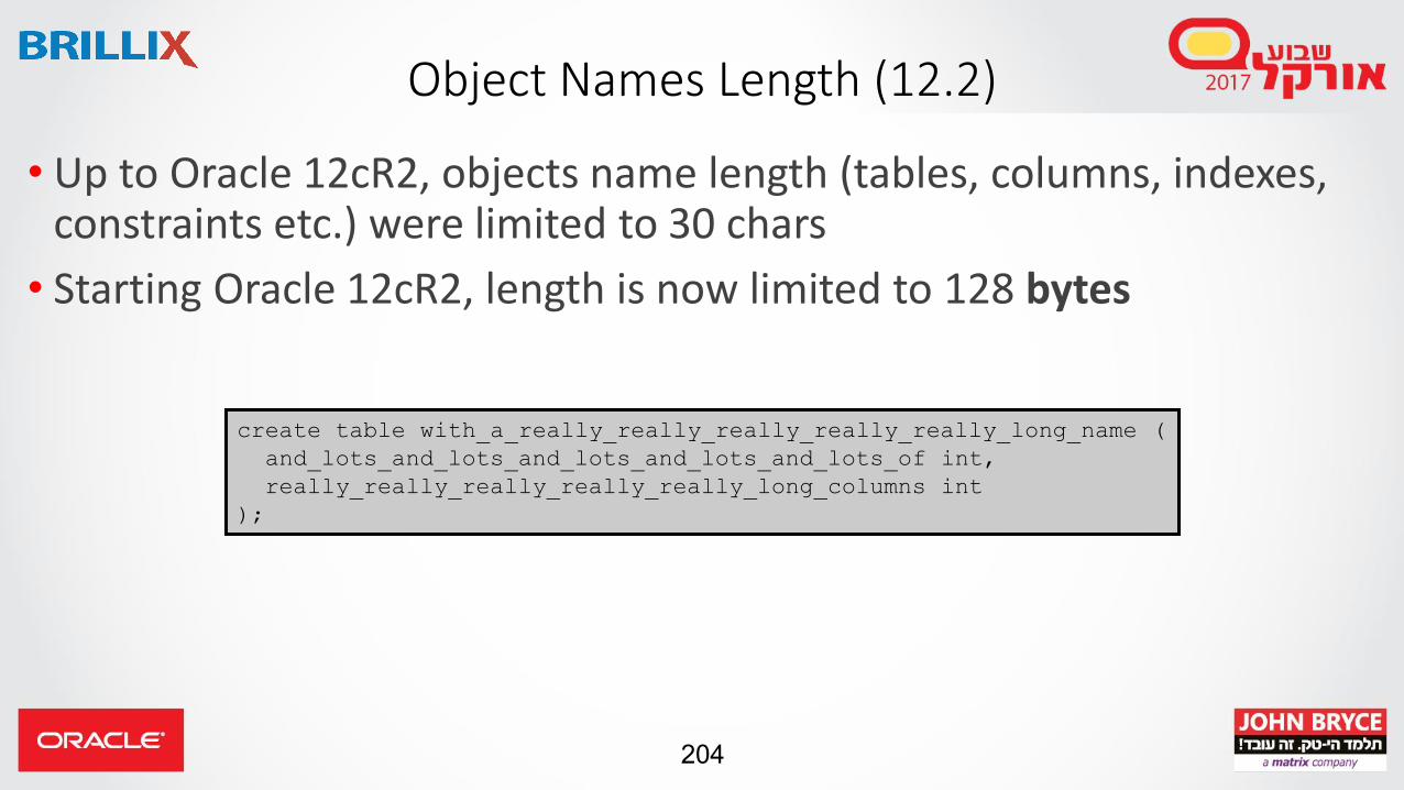
Object Names Length (12.2)
• Up to Oracle 12cR2, objects name length (tables, columns, indexes, constraints etc.) were limited to 30 chars
• Starting Oracle 12cR2, length is now limited to 128 bytes
create table with_a_really_really_really_really_really_long_name (
and_lots_and_lots_and_lots_and_lots_and_lots_of int,
really_really_really_really_really_long_columns int
);

205
Verify Data Type Conversions (12.2)
• If we try to validate using regular conversion we might hit an error: ORA-01858: a non-numeric character was found where a numeric was expected
• Use validate_conversion to validate the data without an error
select t.*
from dodgy_dates t
where validate_conversion(is_this_a_date as date) = 1;
select t.*
from dodgy_dates t
where validate_conversion(is_this_a_date as date, 'yyyymmdd') = 1;

206
Handle Casting Conversion Errors (12.2)
• Let’s say we convert the value of a column using cast. What happens if some of the values doesn’t fit?
• The cast function can now handle conversion errors:
select cast (
'not a date' as date
default date'0001-01-01' on conversion error
) dt
from dual;

207
Approximate Query (12.1)
• APPROX_COUNT_DISTINCT returns the approximate number of rows that contain distinct values of expression
• This gives better performance but might not return the exact result
• Very good for large sets where exact values aren’t significant
• Adjustable using ERROR_RATE and CONFIDENCE parametes

208
Approximate Query Enhancements (12.2)
• 12.2 introduced a parameter, approx_for_count_distinct which automatically replace count distinct with APPROX_COUNT_DISTINCT
• 12.2 also added multiple new approximate functions for example approx_percentile:
approx_percentile (
<expression> [ deterministic ],
[ ('ERROR_RATE' | 'CONFIDENCE') ]
) within group ( order by <expression>)

209
Approximate New Functions (12.2)
• APPROX_COUNT_DISTINCT_AGG• Aggregations of approximate distinct counts
• APPROX_COUNT_DISTINCT_DETAIL• Input values to APPROX_DISTINCT_AGG
• APPROX_MEDIAN• Approximate Median
• APPROX_PERCENTILE• Approximate Percentile
• APPROX_PERCENTILE_AGG• Aggregations of approximate percentiles
• APPROX_PERCENTILE_DETAIL• Input values to APPROX_PERCENT_AGG

210
Approximate Query Performance

211
• Approximate Query Enhancements
• PL/SQL Code Coverage using new DBMS package: dbms_plsql_code_coverage
• Partitions enhancements• List partition major changes: Auto-list, multi-column
• Read only partitions
• More…
More 12c Developers’ Features…

Did You Hear About Oracle 18c?

213
• Oracle is changing the way they number products• Products will be release more often• Version names will be based on last two digits of the year and a
subversion• There is no more Release 1-Release 2 for major versions, we can’t tell
when we jumped to the next major version and when for the next minor• Examples:
• 12.2.0.1 will be followed by 18.1 (and not 12.2.0.2)• SQL Developer 4.2.1 was followed by 17.3
• Read more at the updated MOS Note 742060.1 – Release Schedule of Current Database Releases
Wait! 18c?! What happened to 13c?

214
• Improved JSON support
• Private Temporary Tables (more on that later!)
• Machine Learning Algorithms in the database
• “Autonomous Database”
18c Developers’ Features (preview)
SQLcl IntroductionThe Next Generation of SQL*Plus?

216
SQL*Plus
• Introduced in Oracle 5 (1985)
• Looks very simple but has tight integration with other Oracle infrastructure and tools
• Very good for reporting, scripting, and automation
• Replaced old CLI tool called …
UFI (“User Friendly Interface”)

217
What’s Wrong With SQL*Plus?
• Nothing really wrong with SQL*Plus – it is being updated constantly but it is missing a lot of functionality
• SQL*Plus forces us to use GUI tools to complete some basic tasks
• Easy to understand, a bit hard to use
• Not easy for new users or developers

218
Using SQL Developer
• SQL Developer is a free GUI tool to handle common database operations
• Comes with Oracle client installation starting Oracle 11g
• Good for development and management of databases • Developer mode
• DBA mode
• Modeling mode
• Has a Command Line interface (SDCLI) – but it’s not interactive

219
SQL Developer Command Line (SQLcl)
• The SQL Developer Command Line (SQLcl, priv. SDSQL) is a new command line interface (CLI) for SQL developers, report users, and DBAs
• It is part of the SQL Developer suite – developed by the same team: Oracle Database Development Tools Team
• Does (or will do) most of what SQL*Plus can do, and much more
• Main focus: making life easier for CLI users
• Minimal installation, minimal requirements

220
• Part of 12cR2 Database deployment• current version: 17.3.0.271.1943, September 29, 2017
• New version comes out every couple of months• Adding support for existing SQL*Plus commands/syntax
• Adding new commands and functionality
• The team is accepting bug reports and enhancement requestsfrom the public
• Active community on OTN forums!
Current Status (November 2017)

221
Prerequisites
• Very small footprint: 16 MB
• Tool is Java based so it can run on Windows, Linux, and OS/X
• Java 7/8 JRE (runtime environment - no need for JDK)
• No need for installer or setup
• No need for any other additional software or special license
• No need for an Oracle Client

222
• Download from: SQL Developer Command Line OTN Page
• Unzip the file
• Run it
Installing

223
Running SQLcl

What Can It Do?

225
Connecting to the Database
• When no Oracle Client - using thin connection: EZConnect connect style out of the box
connect host:port/service
• Support TNS, Thick and LDAP connection when Oracle home detected
• Auto-complete connection strings from last connections AND tnsnames.ora
226
Object Completion and Easy Edit
• Use the tab key to complete commands
• Can be used to list tables, views or other queriable objects
• Can be used to replace the * with actual column names
• Use the arrow keys to move around the command
• Use CTRL+W and CTRL+S to jump to the beginning/end of commands

227
Command History
• 100 command history buffer• Commands are persistent between sessions (watch out for security!)• Use UP and DOWN arrow keys to access old commands• Usage:historyhistory usageHistory scripthistory fullHistory clear [session?]
• Load from history into command buffer:history <number>

228
Describe, Information and Info+
• Describe lists the column of the tables just like SQL*Plus
• Information shows column names, default values, indexes and constraints.
• In 12c database information shows table statistics and In memory status
• Works for table, views, sequences, and code objects
• Info+ shows additional information regarding column statistics and column histograms

229
SHOW ALL and SHOW ALL+
• The show all command is familiar from SQL*Plus – it will show all the parameters for the SQL*Plus settings
• The show all+ command will show the show all command and some perks: available tns entries, list of pdbs, connection settings, instance settings, nls settings, and more!

230
Pretty Input
• Using the SQL Developer formatting rules, it will change our input into well formatted commands.
• Use the SQLFORMATPATH to point to the SQL Developer rule file (XML)
SQL> select * from dual;
D-X
SQL> format buffer;1 SELECT2 *3 FROM4* dual

231
SQL*Plus Output
• SQL*Plus output is generated as text tables
• We can output the data as HTML but the will take over everything we do in SQL*Plus (i.e. describe command)
• We can’t use colors in our output
• We can’t generate other types of useful outputs (CSV is really hard for example)
232
Generating Pretty Output
• Outputting query results becomes easier with the “set sqlformat” command (also available in SQL Developer)
• We can create a query in the “regular” way and then switch between the different output styles:
• ANSIConsole
• Fixed column size output
• XML or JSON output
• HTML output generates a built in search field and a responsive html output for the result only

233
Generating Other Useful Outputs
• We can generate loader ready output (with “|” as a delimiter)
• We can generate insert commands
• We can easily generate CSV output
• Usage:set sqlformat { csv,html,xml,json,ansiconsole,insert,loader,fixed,default}

234
Load Data From CSV File
• Loads a comma separated value (csv) file into a table
• The first row of the file must be a header row and the file must be encoded UTF8
• The load is processed with 50 rows per batch
• Usage:LOAD [schema.]table_name[@db_link] file_name

235
SCRIPT – Client Side Scripting
• SQLcl exposes JavaScript scripting with nashorn to make things very scriptable on the client side
• This means we can create our own commands inside SQLcl using JavaScript
• Kris Rice’s from the development team published multiple example on his blog http://krisrice.blogspot.com/ and in GitHub, for example the autocorrect example demo.

236
Summary
• There is a lot in SQL than meets the eye
• Wise use of analytic queries can be good for readability and performance
• Recursive queries are good replacement for the old connect by prior but a little dangerous
• Oracle 12c features are really cool!
• Look out for SQLcl: it’s cool and it’s going places!
237
What Did We Not Talk About?
• The Model clause
• Adding PL/SQL to our SQL (Oracle 12c)
• Hints and other tuning considerations
• The SQL reference book is 1906 pages long. We didn’t talk about most of it…

Q&AAny Questions? Now will be the time!