Smooth Entropies — A TutorialWith Focus on Applications in Cryptography.

Marco Tomamichel

CQT, National University of Singapore

Singapore, September 14, 2011

1 / 53

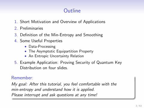
Outline

1. Short Motivation and Overview of Applications

2. Preliminaries

3. Definition of the Min-Entropy and Smoothing

4. Some Useful Properties• Data-Processing• The Asymptotic Equipartition Property• An Entropic Uncertainty Relation

5. Example Application: Proving Security of Quantum KeyDistribution on four slides.

Remember:

My goal: After this tutorial, you feel comfortable with themin-entropy and understand how it is applied.Please interrupt and ask questions at any time!

2 / 53

Motivation and OverviewJust a quick overview.

3 / 53

Entropic Approach to Information I

• Probability theory offers many advantages to describecryptographic problems.

• For example, how do we describe a secret key?

X = ”01010100100111001110100”

Is this string secret? From whom? We cannot tell unless weknow how it is created.

• Instead, we look at the joint probability distribution overpotential strings and side information, PXE . Here, E is anyinformation a potential adversary might hold about X .

• If PX is uniform and independent of E , we call it secret.

4 / 53

Entropic Approach to Information II

• We can also describe this situation with entropy [Sha48].

• Shannon defined the surprisal of an event X = x asS(x)P = − log P(x).

• We can thus call a string secret if the average surprisal,H(X )P =

∑x P(x)S(x)P , is large.

• Entropies are measures of uncertainty about (the value of) arandom variable.

• There are other entropies, for example the min-entropy orRenyi entropy [Ren61] of order ∞.

Hmin(X ) = minx

S(x)P .

• The min-entropy quantifies how hard it is to guess X . (Theoptimal guessing strategy is to guess the most likely event,and the probability of success is pguess(X )P = 2−Hmin(X )P .)

5 / 53

Entropic Approach to Information III

• Entropies can be easily extended to (classical) sideinformation, using conditional probability distributions.

• In the quantum setting, conditional states are not available(there exist some definitions, but none of them appear veryuseful) and the entropic approach is often the only availableoption to quantify information.

• The von Neumann entropy generalizes Shannon’s entropy tothe quantum setting,

H(A|B)ρ := H(ρAB)− H(ρB), H(ρ) = −tr(ρ log ρ).

• This tutorial is concerned with a quantum extension of themin-entropy.

6 / 53

Foundations

• The quantum generalization of the conditional min- andmax-entropy was introduced by Renner [Ren05] in his thesis.

• The main purpose was to generalize a theorem on privacyamplification to the quantum setting.

• Since then, the smooth entropy framework has beenconsolidated and extended [Tom12].• The definition of Hmax is not what it used to be [KRS09].• The smoothing is now done with regards to the purified

distance [TCR10].

• A relative entropy based on the quantum generalization of themin-entropy was introduced by Datta [Dat09].

7 / 53

Applications

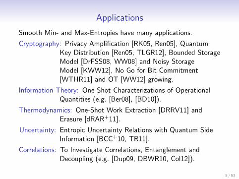
Smooth Min- and Max-Entropies have many applications.

Cryptography: Privacy Amplification [RK05, Ren05], QuantumKey Distribution [Ren05, TLGR12], Bounded StorageModel [DrFSS08, WW08] and Noisy StorageModel [KWW12], No Go for Bit Commitment[WTHR11] and OT [WW12] growing.

Information Theory: One-Shot Characterizations of OperationalQuantities (e.g. [Ber08], [BD10]).

Thermodynamics: One-Shot Work Extraction [DRRV11] andErasure [dRAR+11].

Uncertainty: Entropic Uncertainty Relations with Quantum SideInformation [BCC+10, TR11].

Correlations: To Investigate Correlations, Entanglement andDecoupling (e.g. [Dup09, DBWR10, Col12]).

8 / 53

Mathematical PreliminariesStay with me through this part, after which I hope everybody is onthe same level.

9 / 53

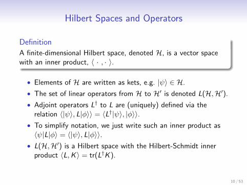
Hilbert Spaces and Operators

Definition

A finite-dimensional Hilbert space, denoted H, is a vector spacewith an inner product, 〈 · , · 〉.

• Elements of H are written as kets, e.g. |ψ〉 ∈ H.

• The set of linear operators from H to H′ is denoted L(H,H′).

• Adjoint operators L† to L are (uniquely) defined via therelation 〈|ψ〉, L|φ〉〉 = 〈L†|ψ〉, |φ〉〉.

• To simplify notation, we just write such an inner product as〈ψ|L|φ〉 = 〈|ψ〉, L|φ〉〉.

• L(H,H′) is a Hilbert space with the Hilbert-Schmidt innerproduct 〈L,K 〉 = tr(L†K ).

10 / 53

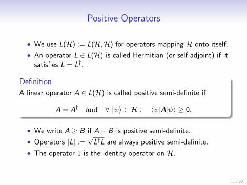
Positive Operators

• We use L(H) := L(H,H) for operators mapping H onto itself.

• An operator L ∈ L(H) is called Hermitian (or self-adjoint) if itsatisfies L = L†.

Definition

A linear operator A ∈ L(H) is called positive semi-definite if

A = A† and ∀ |ψ〉 ∈ H : 〈ψ|A|ψ〉 ≥ 0.

• We write A ≥ B if A− B is positive semi-definite.

• Operators |L| :=√

L†L are always positive semi-definite.

• The operator 1 is the identity operator on H.

11 / 53

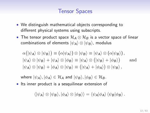
Tensor Spaces

• We distinguish mathematical objects corresponding todifferent physical systems using subscripts.

• The tensor product space HA ⊗HB is a vector space of linearcombinations of elements |ψA〉 ⊗ |ψB〉, modulus

α(|ψA〉 ⊗ |ψB〉

)≡ (α|ψA〉)⊗ |ψB〉 ≡ |ψA〉 ⊗ (α|ψB〉) ,

|ψA〉 ⊗ |ψB〉+ |ψA〉 ⊗ |φB〉 ≡ |ψA〉 ⊗(|ψB〉+ |φB〉

)and

|ψA〉 ⊗ |ψB〉+ |φA〉 ⊗ |ψB〉 ≡(|ψA〉+ |φA〉

)⊗ |ψB〉 ,

where |ψA〉, |φA〉 ∈ HA and |ψB〉, |φB〉 ∈ HB .

• Its inner product is a sesquilinear extension of

〈|ψA〉 ⊗ |ψB〉, |φA〉 ⊗ |φB〉〉 = 〈ψA|φA〉 〈ψB |φB〉 .

12 / 53

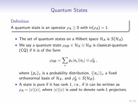
Quantum States

Definition

A quantum state is an operator ρA ≥ 0 with tr(ρA) = 1.

• The set of quantum states on a Hilbert space HA is S(HA).

• We say a quantum state ρXB ∈ HX ⊗HB is classical-quantum(CQ) if it is of the form

ρXB =∑

x

px |ex〉〈ex | ⊗ ρxB ,

where {px}x is a probability distribution, {|ex〉}x a fixedorthonormal basis of HX , and ρx

B ∈ S(HB).

• A state is pure if it has rank 1, i.e., if it can be written asρA = |ψ〉〈ψ|, where |ψ〉〈ψ| is used to denote rank-1 projectors.

13 / 53

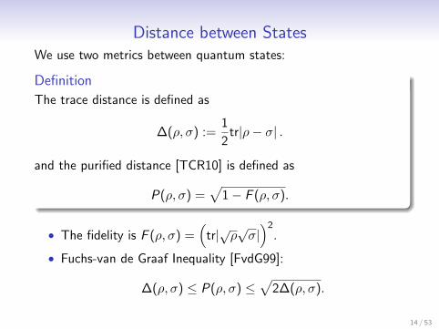
Distance between StatesWe use two metrics between quantum states:

Definition

The trace distance is defined as

∆(ρ, σ) :=1

2tr|ρ− σ| .

and the purified distance [TCR10] is defined as

P(ρ, σ) =√

1− F (ρ, σ).

• The fidelity is F (ρ, σ) =(

tr|√ρ√σ|)2

.

• Fuchs-van de Graaf Inequality [FvdG99]:

∆(ρ, σ) ≤ P(ρ, σ) ≤√

2∆(ρ, σ).

14 / 53

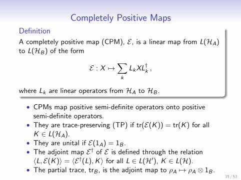
Completely Positive Maps

Definition

A completely positive map (CPM), E , is a linear map from L(HA)to L(HB) of the form

E : X 7→∑

k

Lk XL†k ,

where Lk are linear operators from HA to HB .

• CPMs map positive semi-definite operators onto positivesemi-definite operators.

• They are trace-preserving (TP) if tr(E(K )) = tr(K ) for allK ∈ L(HA).

• They are unital if E(1A) = 1B .• The adjoint map E† of E is defined through the relation〈L, E(K )〉 = 〈E†(L),K 〉 for all L ∈ L(H′), K ∈ L(H).

• The partial trace, trB , is the adjoint map to ρA 7→ ρA ⊗ 1B .15 / 53

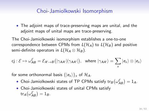
Choi-Jamiolkowski Isomorphism

• The adjoint maps of trace-preserving maps are unital, and theadjoint maps of unital maps are trace-preserving.

The Choi-Jamiolkowski isomorphism establishes a one-to-onecorrespondence between CPMs from L(HA) to L(HB) and positivesemi-definite operators in L(HA ⊗HB).

cj : E 7→ ωEAB = EA′→B

(|γAA′〉〈γAA′ |

), where |γAA′〉 =

∑x

|ex〉 ⊗ |ex〉

for some orthonormal basis {|ex〉}x of HA.

• Choi-Jamiolkowski states of TP CPMs satisfy trB

(ωEAB

)= 1A.

• Choi-Jamiolkowski states of unital CPMs satisfytrA

(ωEAB

)= 1B .

16 / 53

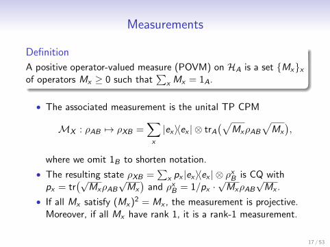
Measurements

Definition

A positive operator-valued measure (POVM) on HA is a set {Mx}x

of operators Mx ≥ 0 such that∑

x Mx = 1A.

• The associated measurement is the unital TP CPM

MX : ρAB 7→ ρXB =∑

x

|ex〉〈ex | ⊗ trA

(√MxρAB

√Mx

),

where we omit 1B to shorten notation.

• The resulting state ρXB =∑

x px |ex〉〈ex | ⊗ ρxB is CQ with

px = tr(√

MxρAB

√Mx

)and ρx

B = 1/px ·√

MxρAB

√Mx .

• If all Mx satisfy (Mx )2 = Mx , the measurement is projective.Moreover, if all Mx have rank 1, it is a rank-1 measurement.

17 / 53

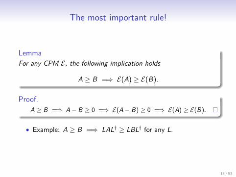
The most important rule!

Lemma

For any CPM E , the following implication holds

A ≥ B =⇒ E(A) ≥ E(B).

Proof.

A ≥ B =⇒ A− B ≥ 0 =⇒ E(A− B) ≥ 0 =⇒ E(A) ≥ E(B).

• Example: A ≥ B =⇒ LAL† ≥ LBL† for any L.

18 / 53

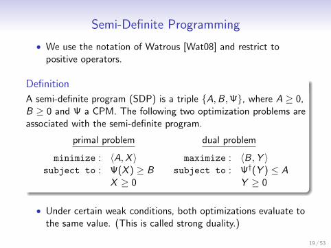
Semi-Definite Programming

• We use the notation of Watrous [Wat08] and restrict topositive operators.

Definition

A semi-definite program (SDP) is a triple {A,B,Ψ}, where A ≥ 0,B ≥ 0 and Ψ a CPM. The following two optimization problems areassociated with the semi-definite program.

primal problem dual problem

minimize : 〈A,X 〉 maximize : 〈B,Y 〉subject to : Ψ(X ) ≥ B subject to : Ψ†(Y ) ≤ A

X ≥ 0 Y ≥ 0

• Under certain weak conditions, both optimizations evaluate tothe same value. (This is called strong duality.)

19 / 53

The Min-Entropy and GuessingNow it gets more interesting.

20 / 53

Min-Entropy: Definition

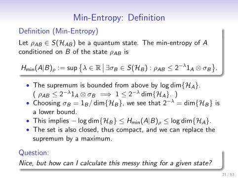
Definition (Min-Entropy)

Let ρAB ∈ S(HAB) be a quantum state. The min-entropy of Aconditioned on B of the state ρAB is

Hmin(A|B)ρ := sup{λ ∈ R

∣∣∃σB ∈ S(HB) : ρAB ≤ 2−λ1A ⊗ σB

}.

• The supremum is bounded from above by log dim{HA}.( ρAB ≤ 2−λ1A ⊗ σB =⇒ 1 ≤ 2−λ dim{HA}. )

• Choosing σB = 1B/ dim{HB}, we see that 2−λ = dim{HB} isa lower bound.

• This implies − log dim{HB} ≤ Hmin(A|B)ρ ≤ log dim{HA}.• The set is also closed, thus compact, and we can replace the

supremum by a maximum.

Question:

Nice, but how can I calculate this messy thing for a given state?

21 / 53

Min-Entropy: SDP I

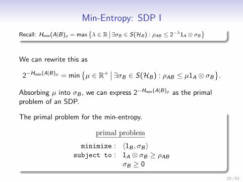
Recall: Hmin(A|B)ρ = max{λ ∈ R

∣∣ ∃σB ∈ S(HB ) : ρAB ≤ 2−λ1A ⊗ σB

}

We can rewrite this as

2−Hmin(A|B)ρ = min{µ ∈ R+

∣∣∃σB ∈ S(HB) : ρAB ≤ µ1A ⊗ σB

}.

Absorbing µ into σB , we can express 2−Hmin(A|B)ρ as the primalproblem of an SDP.

The primal problem for the min-entropy.

primal problem

minimize : 〈1B , σB〉subject to : 1A ⊗ σB ≥ ρAB

σB ≥ 0

22 / 53

Min-Entropy: SDP II

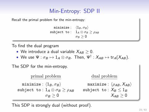
Recall the primal problem for the min-entropy:

minimize : 〈1B , σB〉subject to : 1A ⊗ σB ≥ ρAB

σB ≥ 0

To find the dual program• We introduce a dual variable XAB ≥ 0.• We use Ψ : σB 7→ 1A ⊗ σB . Then, Ψ† : XAB 7→ trA(XAB).

The SDP for the min-entropy.

primal problem dual problem

minimize : 〈1B , σB〉 maximize : 〈ρAB ,XAB〉subject to : 1A ⊗ σB ≥ ρAB subject to : XB ≤ 1B

σB ≥ 0 XAB ≥ 0

This SDP is strongly dual (without proof).23 / 53

Min-Entropy: SDP III

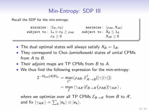
Recall the SDP for the min-entropy:

minimize : 〈1B , σB〉 maximize : 〈ρAB ,XAB〉subject to : 1A ⊗ σB ≥ ρAB subject to : XB ≤ 1B

σB ≥ 0 XAB ≥ 0

• The dual optimal states will always satisfy XB = 1B .• They correspond to Choi-Jamiolkowski states of unital CPMs

from A to B.• Their adjoint maps are TP CPMs from B to A.• We thus find the following expression for the min-entropy:

2−Hmin(A|B)ρ = maxE†〈ρAB , E†A′→B(|γ〉〈γ|)〉

= maxE〈γAA′ |EB→A′(ρAB)|γAA′〉 ,

where we optimize over all TP CPMs EB→A′ from B to A′,and fix |γAA′〉 =

∑k |ek〉 ⊗ |ek〉.

24 / 53

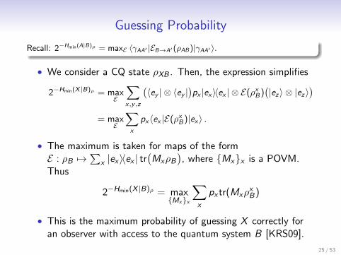
Guessing Probability

Recall: 2−Hmin(A|B)ρ = maxE 〈γAA′ |EB→A′(ρAB )|γAA′〉.

• We consider a CQ state ρXB . Then, the expression simplifies

2−Hmin(X |B)ρ = maxE

∑x,y ,z

(〈ey | ⊗ 〈ey |

)px |ex〉〈ex | ⊗ E(ρx

B )(|ez〉 ⊗ |ez〉

)= max

E

∑x

px〈ex |E(ρxB )|ex〉 .

• The maximum is taken for maps of the formE : ρB 7→

∑x |ex〉〈ex | tr

(MxρB

), where {Mx}x is a POVM.

Thus

2−Hmin(X |B)ρ = max{Mx}x

∑x

px tr(MxρxB)

• This is the maximum probability of guessing X correctly foran observer with access to the quantum system B [KRS09].

25 / 53

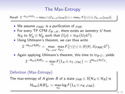
The Max-Entropy

Recall: 2−Hmin(A|B)ρ = maxE〈γ|EB→A′(ρAB )|γ〉= maxE F(|γ〉〈γ|, EB→A′(ρAB )

).

• We assume ρABC is a purification of ρAB .• For every TP CPM EB→A′ , there exists an isometry U fromHB to H′A ⊗H′B such that E(ρ) = trB′(UρU†).

• Using Uhlmann’s theorem, we can thus write

2−Hmin(A|B)ρ = maxUB→A′B′

maxθB′C

F(|γ〉〈γ| ⊗ |θ〉〈θ|,UρABC U†

).

• Again applying Uhlmann’s theorem, this time to trB′C ′ , yields

2−Hmin(A|B)ρ = maxσC

F(1A ⊗ σC , ρAC

)=: 2Hmax(A|C)ρ .

Definition (Max-Entropy)

The max-entropy of A given B of a state ρAB ∈ S(HA ⊗HB) is

Hmax(A|B)ρ := maxσB

log F(1A ⊗ σB , ρAB

).

26 / 53

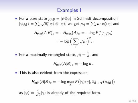
Examples I

• For a pure state ρAB = |ψ〉〈ψ| in Schmidt decomposition|ψAB〉 =

∑i√µi |ei 〉 ⊗ |ei 〉, we get ρA =

∑i µi |ei 〉〈ei | and

Hmin(A|B)ρ = −Hmax(A)ψ = − log F (1A, ρA)

= − log(∑

i

õi

)2.

• For a maximally entangled state, µi = 1d , and

Hmin(A|B)ρ = − log d .

• This is also evident from the expression

Hmin(A|B)ρ = − log maxE

F(|γ〉〈γ|, EB→A′(ρAB)

)as |ψ〉 = 1√

d|γ〉 is already of the required form.

27 / 53

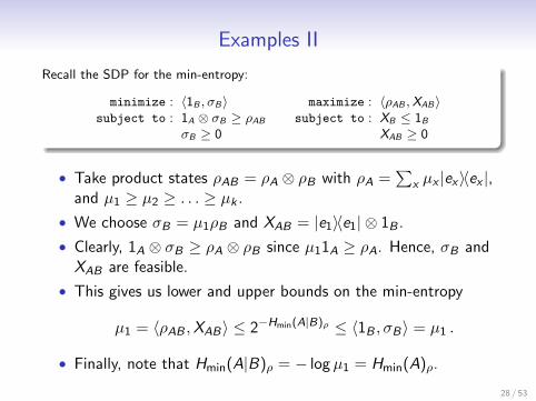
Examples II

Recall the SDP for the min-entropy:

minimize : 〈1B , σB〉 maximize : 〈ρAB ,XAB〉subject to : 1A ⊗ σB ≥ ρAB subject to : XB ≤ 1B

σB ≥ 0 XAB ≥ 0

• Take product states ρAB = ρA ⊗ ρB with ρA =∑

x µx |ex〉〈ex |,and µ1 ≥ µ2 ≥ . . . ≥ µk .

• We choose σB = µ1ρB and XAB = |e1〉〈e1| ⊗ 1B .

• Clearly, 1A ⊗ σB ≥ ρA ⊗ ρB since µ11A ≥ ρA. Hence, σB andXAB are feasible.

• This gives us lower and upper bounds on the min-entropy

µ1 = 〈ρAB ,XAB〉 ≤ 2−Hmin(A|B)ρ ≤ 〈1B , σB〉 = µ1 .

• Finally, note that Hmin(A|B)ρ = − logµ1 = Hmin(A)ρ.

28 / 53

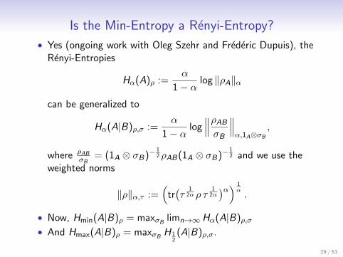
Is the Min-Entropy a Renyi-Entropy?

• Yes (ongoing work with Oleg Szehr and Frederic Dupuis), theRenyi-Entropies

Hα(A)ρ :=α

1− α log ‖ρA‖α

can be generalized to

Hα(A|B)ρ,σ :=α

1− α log∥∥∥ρAB

σB

∥∥∥α,1A⊗σB

,

where ρABσB

= (1A ⊗ σB)−12 ρAB(1A ⊗ σB)−

12 and we use the

weighted norms

‖ρ‖α,τ :=(

tr(τ

12α ρ τ

12α)α) 1

α.

• Now, Hmin(A|B)ρ = maxσBlimn→∞Hα(A|B)ρ,σ

• And Hmax(A|B)ρ = maxσBH 1

2(A|B)ρ,σ.

29 / 53

Smooth Min- and Max-EntropiesAnd their operational interpretation.

30 / 53

Why Smoothing?

1. Most properties of the min- and max-entropy generalize tosmooth entropies.

2. On top of that, the smooth entropies have additionalproperties. Most prominently, they satisfy an entropicequipartition law which relates them to the conditional vonNeumann entropy.

3. The smoothing parameter has operational meaning in someapplications, for example, the ε-smooth min-entropycharacterizes how much ε-close to uniform randomness can beextracted from a random variable.

4. The smooth entropies allow us to exclude improbable events.A statistical analysis performed on a random sample of statesmay thus allow us to bound a smooth entropy, but not(directly) the actual min- or max-entropy.

31 / 53

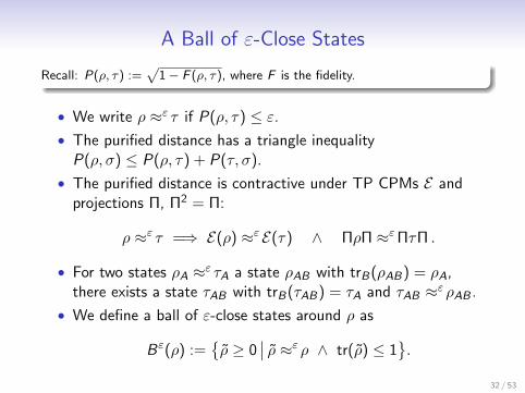
A Ball of ε-Close States

Recall: P(ρ, τ) :=√

1− F (ρ, τ), where F is the fidelity.

• We write ρ ≈ε τ if P(ρ, τ) ≤ ε.

• The purified distance has a triangle inequalityP(ρ, σ) ≤ P(ρ, τ) + P(τ, σ).

• The purified distance is contractive under TP CPMs E andprojections Π, Π2 = Π:

ρ ≈ε τ =⇒ E(ρ) ≈εE(τ) ∧ ΠρΠ ≈εΠτΠ .

• For two states ρA ≈ε τA a state ρAB with trB(ρAB) = ρA,there exists a state τAB with trB(τAB) = τA and τAB ≈ε ρAB .

• We define a ball of ε-close states around ρ as

Bε(ρ) :={ρ ≥ 0

∣∣ ρ ≈ε ρ ∧ tr(ρ) ≤ 1}.

32 / 53

Smooth Entropies

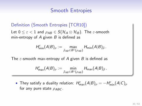
Definition (Smooth Entropies [TCR10])

Let 0 ≤ ε < 1 and ρAB ∈ S(HA ⊗HB). The ε-smoothmin-entropy of A given B is defined as

Hεmin(A|B)ρ := max

ρAB∈Bε(ρAB )Hmin(A|B)ρ .

The ε-smooth max-entropy of A given B is defined as

Hεmax(A|B)ρ := min

ρAB∈Bε(ρAB )Hmax(A|B)ρ .

• They satisfy a duality relation: Hεmax(A|B)ρ = −Hε

min(A|C )ρfor any pure state ρABC .

33 / 53

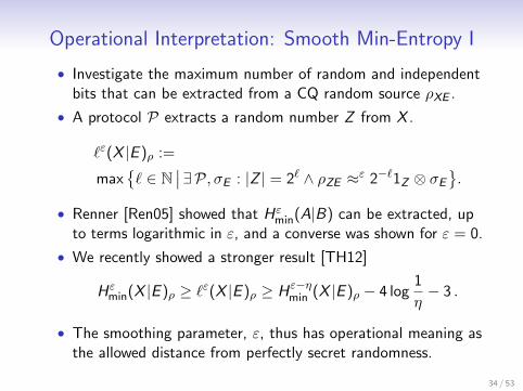
Operational Interpretation: Smooth Min-Entropy I

• Investigate the maximum number of random and independentbits that can be extracted from a CQ random source ρXE .

• A protocol P extracts a random number Z from X .

`ε(X |E )ρ :=

max{` ∈ N

∣∣∃P, σE : |Z | = 2` ∧ ρZE ≈ε 2−`1Z ⊗ σE

}.

• Renner [Ren05] showed that Hεmin(A|B) can be extracted, up

to terms logarithmic in ε, and a converse was shown for ε = 0.

• We recently showed a stronger result [TH12]

Hεmin(X |E )ρ ≥ `ε(X |E )ρ ≥ Hε−η

min (X |E )ρ − 4 log1

η− 3 .

• The smoothing parameter, ε, thus has operational meaning asthe allowed distance from perfectly secret randomness.

34 / 53

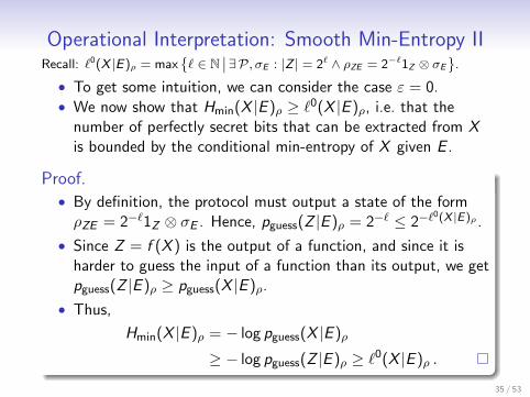
Operational Interpretation: Smooth Min-Entropy IIRecall: `0(X |E)ρ = max

{` ∈ N

∣∣∃P, σE : |Z | = 2` ∧ ρZE = 2−`1Z ⊗ σE

}.

• To get some intuition, we can consider the case ε = 0.• We now show that Hmin(X |E )ρ ≥ `0(X |E )ρ, i.e. that the

number of perfectly secret bits that can be extracted from Xis bounded by the conditional min-entropy of X given E .

Proof.• By definition, the protocol must output a state of the formρZE = 2−`1Z ⊗ σE . Hence, pguess(Z |E )ρ = 2−` ≤ 2−`

0(X |E)ρ .

• Since Z = f (X ) is the output of a function, and since it isharder to guess the input of a function than its output, we getpguess(Z |E )ρ ≥ pguess(X |E )ρ.

• Thus,

Hmin(X |E )ρ = − log pguess(X |E )ρ

≥ − log pguess(Z |E )ρ ≥ `0(X |E )ρ .

35 / 53

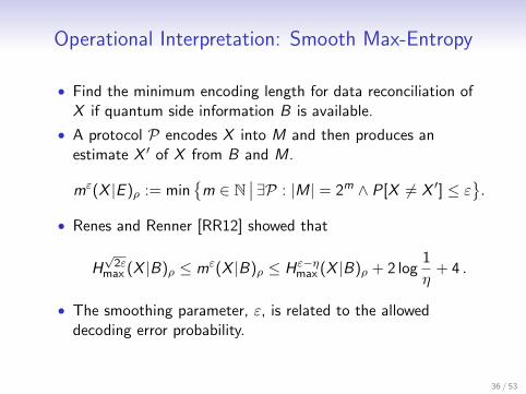
Operational Interpretation: Smooth Max-Entropy

• Find the minimum encoding length for data reconciliation ofX if quantum side information B is available.

• A protocol P encodes X into M and then produces anestimate X ′ of X from B and M.

mε(X |E )ρ := min{

m ∈ N∣∣∃P : |M| = 2m ∧ P[X 6= X ′] ≤ ε

}.

• Renes and Renner [RR12] showed that

H√

2εmax (X |B)ρ ≤ mε(X |B)ρ ≤ Hε−η

max (X |B)ρ + 2 log1

η+ 4 .

• The smoothing parameter, ε, is related to the alloweddecoding error probability.

36 / 53

Basic Properties of Smooth Entropies

37 / 53

Asymptotic Equipartition

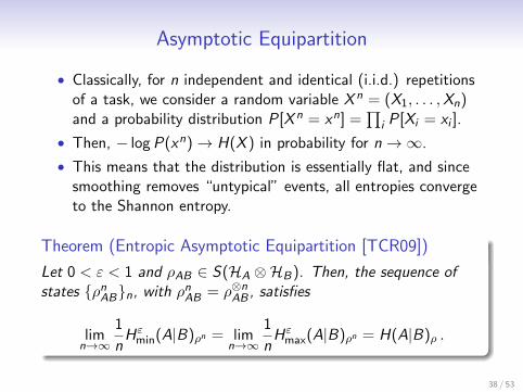
• Classically, for n independent and identical (i.i.d.) repetitionsof a task, we consider a random variable X n = (X1, . . . ,Xn)and a probability distribution P[X n = xn] =

∏i P[Xi = xi ].

• Then, − log P(xn)→ H(X ) in probability for n→∞.

• This means that the distribution is essentially flat, and sincesmoothing removes “untypical” events, all entropies convergeto the Shannon entropy.

Theorem (Entropic Asymptotic Equipartition [TCR09])

Let 0 < ε < 1 and ρAB ∈ S(HA ⊗HB). Then, the sequence ofstates {ρn

AB}n, with ρnAB = ρ⊗n

AB , satisfies

limn→∞

1

nHε

min(A|B)ρn = limn→∞

1

nHε

max(A|B)ρn = H(A|B)ρ .

38 / 53

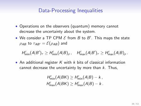
Data-Processing Inequalities

• Operations on the observers (quantum) memory cannotdecrease the uncertainty about the system.

• We consider a TP CPM E from B to B ′. This maps the stateρAB to τAB′ = E(ρAB) and

Hεmin(A|B ′)τ ≥ Hε

min(A|B)ρ , Hεmax(A|B ′)τ ≥ Hε

max(A|B)ρ .

• An additional register K with k bits of classical informationcannot decrease the uncertainty by more than k . Thus,

Hεmin(A|BK ) ≥ Hε

min(A|B)− k ,

Hεmax(A|BK ) ≥ Hε

max(A|B)− k .

39 / 53

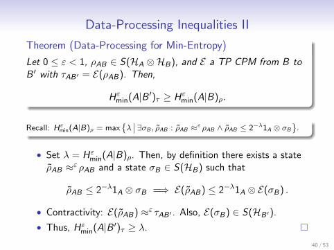
Data-Processing Inequalities II

Theorem (Data-Processing for Min-Entropy)

Let 0 ≤ ε < 1, ρAB ∈ S(HA ⊗HB), and E a TP CPM from B toB ′ with τAB′ = E(ρAB). Then,

Hεmin(A|B ′)τ ≥ Hε

min(A|B)ρ.

Recall: Hεmin(A|B)ρ = max{λ∣∣ ∃σB , ρAB : ρAB ≈ε ρAB ∧ ρAB ≤ 2−λ1A ⊗ σB

}.

• Set λ = Hεmin(A|B)ρ. Then, by definition there exists a state

ρAB ≈ε ρAB and a state σB ∈ S(HB) such that

ρAB ≤ 2−λ1A ⊗ σB =⇒ E(ρAB) ≤ 2−λ1A ⊗ E(σB) .

• Contractivity: E(ρAB) ≈ε τAB′ . Also, E(σB) ∈ S(HB′).

• Thus, Hεmin(A|B ′)τ ≥ λ.

40 / 53

Entropic Uncertainty IGiven Θ, what is X?

bb

bb

b

b

b

ρ

Θ ∈ {+,×}

X

uniform

O1

O2

bb

bb

b

b

b

bb

bb

b

b

b

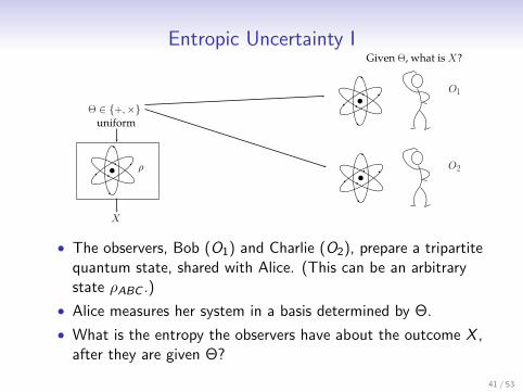
• The observers, Bob (O1) and Charlie (O2), prepare a tripartitequantum state, shared with Alice. (This can be an arbitrarystate ρABC .)

• Alice measures her system in a basis determined by Θ.

• What is the entropy the observers have about the outcome X ,after they are given Θ?

41 / 53

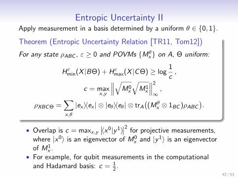
Entropic Uncertainty IIApply measurement in a basis determined by a uniform θ ∈ {0, 1}.Theorem (Entropic Uncertainty Relation [TR11, Tom12])

For any state ρABC , ε ≥ 0 and POVMs {Mθx } on A, Θ uniform:

Hεmin(X |BΘ) + Hε

max(X |C Θ) ≥ log1

c,

c = maxx ,y

∥∥∥√M0x

√M1

x

∥∥∥2

∞,

ρXBCΘ =∑x ,θ

|ex〉〈ex | ⊗ |eθ〉〈eθ| ⊗ trA

((Mθ

x ⊗ 1BC )ρABC

).

• Overlap is c = maxx ,y

∣∣〈x0|y 1〉∣∣2 for projective measurements,

where |x0〉 is an eigenvector of M0x and |y 1〉 is an eigenvector

of M1x .

• For example, for qubit measurements in the computationaland Hadamard basis: c = 1

2 .42 / 53

Entropic Uncertainty III

• This can be lifted to n independent measurements, eachchosen at random.

Hεmin(X n|BΘn) + Hε

max(X n|C Θn) ≥ n log1

c.

• This implies previous uncertainty relations for the vonNeumann entropy [BCC+10] via asymptotic equipartition.• For this, we apply the above relation to product statesρn

ABC = ρ⊗nABC .

• Then, we divide by n and use

1

nHε

min/max(X n|BnΘn)n→∞−−−−→ H(X |BΘ) .

This yields H(X |BΘ) + H(X |C Θ) ≥ log 1c in the limit.

43 / 53

Quantum Key DistributionAn attempt to prove security on 4 slides.(Asymptotically, and trusting our devices to some degree...)

44 / 53

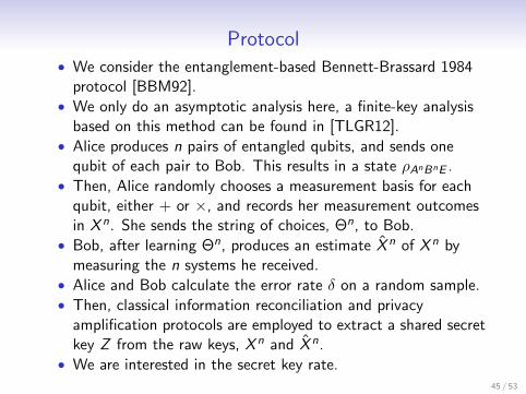
Protocol• We consider the entanglement-based Bennett-Brassard 1984

protocol [BBM92].• We only do an asymptotic analysis here, a finite-key analysis

based on this method can be found in [TLGR12].• Alice produces n pairs of entangled qubits, and sends one

qubit of each pair to Bob. This results in a state ρAnBnE .• Then, Alice randomly chooses a measurement basis for each

qubit, either + or ×, and records her measurement outcomesin X n. She sends the string of choices, Θn, to Bob.

• Bob, after learning Θn, produces an estimate X n of X n bymeasuring the n systems he received.

• Alice and Bob calculate the error rate δ on a random sample.• Then, classical information reconciliation and privacy

amplification protocols are employed to extract a shared secretkey Z from the raw keys, X n and X n.

• We are interested in the secret key rate.45 / 53

Security Analysis I

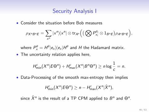
• Consider the situation before Bob measures

ρX nBnE =∑xn

|xn〉〈xn| ⊗ trAn

((⊗Pθi

xi⊗ 1BnE

)ρAnBnE

),

where Pθx = Hθ|ex〉〈ex |Hθ and H the Hadamard matrix.

• The uncertainty relation applies here,

Hεmin(X n|E Θn) + Hε

max(X n|BnΘn) ≥ n log1

c= n.

• Data-Processing of the smooth max-entropy then implies

Hεmin(X n|E Θn) ≥ n − Hε

max(X n|X n),

since X n is the result of a TP CPM applied to Bn and Θn.

46 / 53

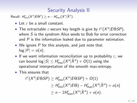
Security Analysis IIRecall: Hεmin(X n|EΘn) ≥ n − Hεmax(X n|X n).

• Let ε be a small constant.

• The extractable ε-secure key length is give by `ε(X n|E ΘSP),where S is the syndrom Alice sends to Bob for error correctionand P is the information leaked due to parameter estimation.

• We ignore P for this analysis, and just note thatlog |P| = o(n).

• If we want information reconciliation up to probability ε, wecan bound log |S | ≤ Hε

max(X n|X n) + O(1) using theoperational interpretation of the smooth max-entropy.

• This ensures that

`ε(X n|E ΘSP) ≥ Hεmin(X n|E ΘSP) + O(1)

≥ Hεmin(X n|E Θ)− Hε

max(X n|X n) + o(n)

≥ n − 2Hεmax(X n|X n) + o(n).

47 / 53

Security Analysis III

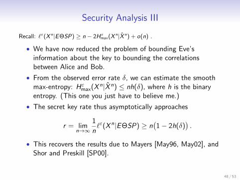
Recall: `ε(X n|EΘSP) ≥ n − 2Hεmax(X n|X n) + o(n) .

• We have now reduced the problem of bounding Eve’sinformation about the key to bounding the correlationsbetween Alice and Bob.

• From the observed error rate δ, we can estimate the smoothmax-entropy: Hε

max(X n|X n) ≤ nh(δ), where h is the binaryentropy. (This one you just have to believe me.)

• The secret key rate thus asymptotically approaches

r = limn→∞

1

n`ε(X n|E ΘSP) ≥ n

(1− 2h(δ)

).

• This recovers the results due to Mayers [May96, May02], andShor and Preskill [SP00].

48 / 53

Conclusion

• The entropic approach to quantum information is verypowerful, especially in cryptography.

• The smooth entropies are universal, they have many usefulproperties (I discussed only a small fraction of them here) andclear operational meaning.

• The smooth entropy formalism leads to an intuitive securityproof for QKD, which also naturally yields finite key bounds.

49 / 53

Thank you for your attention.

50 / 53

Bibliography I[BBM92] Charles H. Bennett, Gilles Brassard, and N. D. Mermin, Quantum cryptography without Bells

theorem, Phys. Rev. Lett. 68 (1992), no. 5, 557–559.

[BCC+10] Mario Berta, Matthias Christandl, Roger Colbeck, Joseph M. Renes, and Renato Renner, TheUncertainty Principle in the Presence of Quantum Memory, Nat. Phys. 6 (2010), no. 9, 659–662.

[BD10] Francesco Buscemi and Nilanjana Datta, The Quantum Capacity of Channels With ArbitrarilyCorrelated Noise, IEEE Trans. on Inf. Theory 56 (2010), no. 3, 1447–1460.

[Ber08] Mario Berta, Single-Shot Quantum State Merging, Master’s thesis, ETH Zurich, 2008.

[Col12] Patrick J. Coles, Collapse of the quantum correlation hierarchy links entropic uncertainty toentanglement creation.

[Dat09] Nilanjana Datta, Min- and Max- Relative Entropies and a New Entanglement Monotone, IEEE Trans.on Inf. Theory 55 (2009), no. 6, 2816–2826.

[DBWR10] Frederic Dupuis, Mario Berta, Jurg Wullschleger, and Renato Renner, The Decoupling Theorem.

[dRAR+11] Lıdia del Rio, Johan Aberg, Renato Renner, Oscar Dahlsten, and Vlatko Vedral, The ThermodynamicMeaning of Negative Entropy., Nature 474 (2011), no. 7349, 61–3.

[DrFSS08] Ivan B. Damga rd, Serge Fehr, Louis Salvail, and Christian Schaffner, Cryptography in theBounded-Quantum-Storage Model, SIAM J. Comput. 37 (2008), no. 6, 1865.

[DRRV11] Oscar C O Dahlsten, Renato Renner, Elisabeth Rieper, and Vlatko Vedral, Inadequacy of vonNeumann Entropy for Characterizing Extractable Work, New J. Phys. 13 (2011), no. 5, 053015.

[Dup09] Frederic Dupuis, The Decoupling Approach to Quantum Information Theory, Ph.D. thesis, Universitede Montreal, April 2009.

[FvdG99] C.A. Fuchs and J. van de Graaf, Cryptographic distinguishability measures for quantum-mechanicalstates, IEEE Trans. on Inf. Theory 45 (1999), no. 4, 1216–1227.

51 / 53

Bibliography II

[KRS09] Robert Konig, Renato Renner, and Christian Schaffner, The Operational Meaning of Min- andMax-Entropy, IEEE Trans. on Inf. Theory 55 (2009), no. 9, 4337–4347.

[KWW12] Robert Konig, Stephanie Wehner, and Jurg Wullschleger, Unconditional Security From NoisyQuantum Storage, IEEE Trans. on Inf. Theory 58 (2012), no. 3, 1962–1984.

[May96] Dominic Mayers, Quantum Key Distribution and String Oblivious Transfer in Noisy Channels, Proc.CRYPTO, LNCS, vol. 1109, Springer, 1996, pp. 343–357.

[May02] , Shor and Preskill’s and Mayers’s security proof for the BB84 quantum key distributionprotocol, Eur. Phys. J. D 18 (2002), no. 2, 161–170.

[Ren61] A. Renyi, On Measures of Information and Entropy, Proc. Symp. on Math., Stat. and Probability(Berkeley), University of California Press, 1961, pp. 547–561.

[Ren05] Renato Renner, Security of Quantum Key Distribution, Ph.D. thesis, ETH Zurich, December 2005.

[RK05] Renato Renner and Robert Konig, Universally Composable Privacy Amplification Against QuantumAdversaries, Proc. TCC (Cambridge, USA), LNCS, vol. 3378, 2005, pp. 407–425.

[RR12] Joseph M. Renes and Renato Renner, One-Shot Classical Data Compression With Quantum SideInformation and the Distillation of Common Randomness or Secret Keys, IEEE Trans. on Inf. Theory58 (2012), no. 3, 1985–1991.

[Sha48] C. Shannon, A Mathematical Theory of Communication, Bell Syst. Tech. J. 27 (1948), 379–423.

[SP00] Peter Shor and John Preskill, Simple Proof of Security of the BB84 Quantum Key DistributionProtocol, Phys. Rev. Lett. 85 (2000), no. 2, 441–444.

[TCR09] Marco Tomamichel, Roger Colbeck, and Renato Renner, A Fully Quantum Asymptotic EquipartitionProperty, IEEE Trans. on Inf. Theory 55 (2009), no. 12, 5840–5847.

52 / 53

Bibliography III

[TCR10] , Duality Between Smooth Min- and Max-Entropies, IEEE Trans. on Inf. Theory 56 (2010),no. 9, 4674–4681.

[TH12] Marco Tomamichel and Masahito Hayashi, A Hierarchy of Information Quantities for Finite BlockLength Analysis of Quantum Tasks.

[TLGR12] Marco Tomamichel, Charles Ci Wen Lim, Nicolas Gisin, and Renato Renner, Tight Finite-KeyAnalysis for Quantum Cryptography, Nat. Commun. 3 (2012), 634.

[Tom12] Marco Tomamichel, A Framework for Non-Asymptotic Quantum Information Theory, Ph.D. thesis,ETH Zurich, March 2012.

[TR11] Marco Tomamichel and Renato Renner, Uncertainty Relation for Smooth Entropies, Phys. Rev. Lett.106 (2011), no. 11.

[Wat08] John Watrous, Theory of Quantum Information, Lecture Notes, 2008.

[WTHR11] Severin Winkler, Marco Tomamichel, Stefan Hengl, and Renato Renner, Impossibility of GrowingQuantum Bit Commitments, Phys. Rev. Lett. 107 (2011), no. 9.

[WW08] Stephanie Wehner and Jurg Wullschleger, Composable Security in the Bounded-Quantum-StorageModel, Proc. ICALP, LNCS, vol. 5126, Springer, July 2008, pp. 604–615.

[WW12] Severin Winkler and Jurg Wullschleger, On the Efficiency of Classical and Quantum Secure FunctionEvaluation.

53 / 53