Servo Drive for Top Performance | ElmoMC

The Solution For ANY Application

ANY Servo

2

Any Servo, Any Load Elmo Servo Drives incorporate the most advanced Control & Power Conversion Technologies, that in conjunction to Elmo’s Smart & EASy Supporting TOOLs can optimally move any mechanical load scenario.

Elmo’s servo drives meet the machine builder’s continuous expectations for enhanced performance, speed, accuracy, competitiveness, within their budgets.

3

Advanced and extremely fast Vector Control

Results smooth, linear and fast response torque/force.

Electrical frequency (Commutation)> 3kHz

…powerful algorithm enables reaching high electrical speed , yet with no torque degradation at any speed.

Phase Advancing,

Smart control of the Lag- Lead between the BEMF to the current ( Torque/ Speed) for optimum Speed- Torque performance.

Results high speed with constant and stable torque/ Force .

Allows exceeding the speed limits due to Voltage Bus “shortage”.

Strength And Capabilities:

Servo Drives for Any Load

4

High Current bandwidth such as >4.5kHz (Real cases),

Meets toughest servo performance needs…..

Higher Current BW allows higher velocity BW….

Higher velocity BW allow higher position BW…..

Higher current & Velocity & Position BWs allows optimum DUAL Loop performance.

Compensates for loads non linearity and drawbacks.

Very High Current dynamic range of >2000:1

for high resolution Torque/ Force operation allowing very high ratio between lowest to highest torque/ Force.

A 100A Servo Drive still has the full performance at 50 ma.



5

Current Loop Gain Scheduling,

Updates “on the fly” the current loop scheme according to the actual voltage bus.

Results very high gain of the current loop

Very stable Current performance even at extreme bus voltage variations.

In a typical Bus variations the bandwidth is higher by 30% -100%

Significantly Wider bandwidth is accomplished.



6

Automatic Position and Velocity Gain Scheduling

Automatically changing PID parameters and high order filters according to various scenarios .

Results very smooth, stable and fast velocity at different operation scenario and different feedback frequencies.

Adapts velocity control scheme according to load’s and application’s actual instant needs.

Ideal for extreme operation requirements such as very Powerful fast movements with very stable standstill and attenuating External mechanical disturbances.



7

Dual loop.

supports any 2 Feedbacks combination.

Up to 2000:1 resolution ratio between the 2 feedbacks.

Results very high accuracy with moderate cost mechanics motion control.

The Dual Loop high Servo performance results very precise and wide bandwidth operation.

Dual Loop Auto Tuning, “Fast & Easy” optimizing tool.

Simplifies and Reduces the cost of mechanical stage and the cost of motion control components.



8

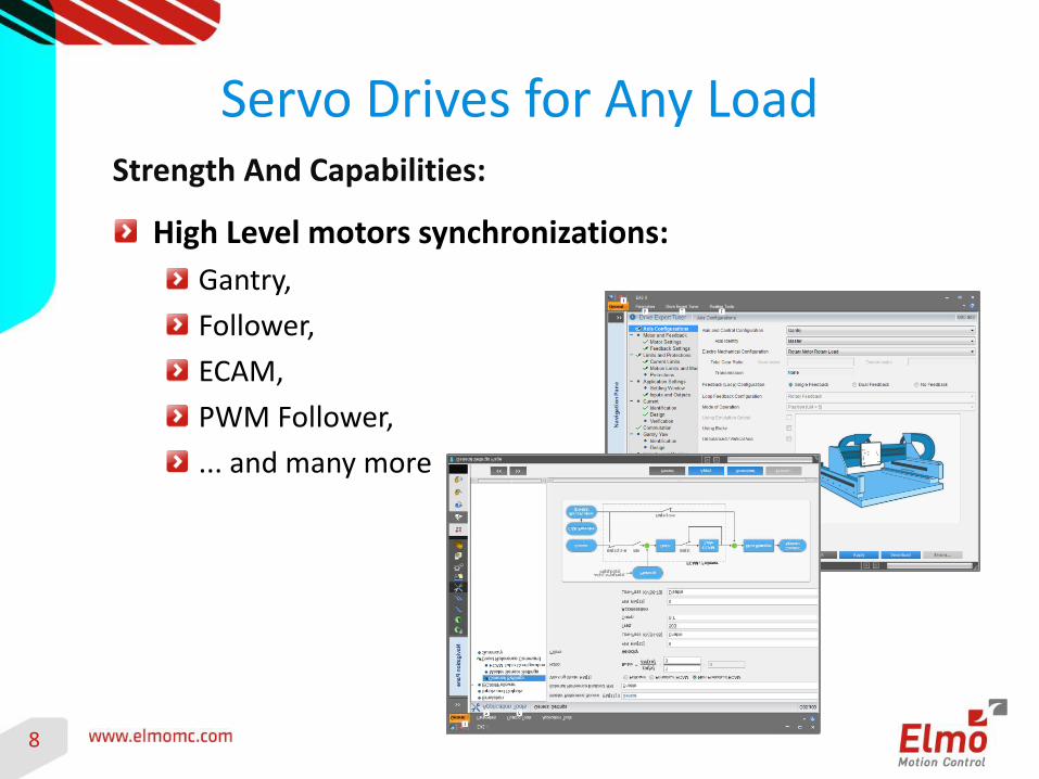
High Level motors synchronizations:

Gantry,

Follower,

ECAM,

PWM Follower,

... and many more



9

Sampling Time Optimizations Controllers sampling rate can be modified to compensate between servo performance, and background tasks performance

Current Loop sampling time down to 50us – 120us (20kHz – 8KHz) Velocity Loop sampling time down to 50us – 120us (20kHz – 8KHz) Position Loop Sampling time down to 50us – 120us (20kHz – 8KHz)

A Rule of Thumb: Faster sampling time allows higher control performance. The sampling time is a mandatory factor for servo performance, but not sufficient. Control algorithms, Power conversion and the TOOLs are even more critical factors.



10

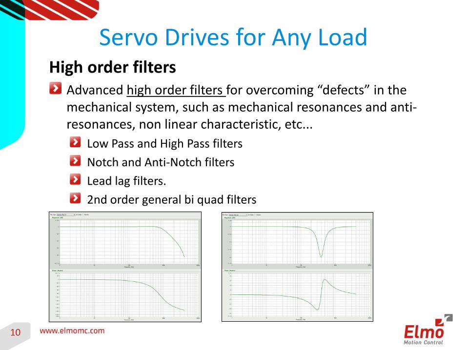
Servo Drives for Any Load High order filters

Advanced high order filters for overcoming “defects” in the mechanical system, such as mechanical resonances and anti-resonances, non linear characteristic, etc...

Low Pass and High Pass filters

Notch and Anti-Notch filters

Lead lag filters.

2nd order general bi quad filters

11

Servo Drives for Any Load Almost Unlimited Optional Filters

More than 10 high orders filters can be used to fine tune the controller:

Low-Pass Filters, Notch / Unti-Notch, Lead-Lag, Double Lead-Lag, or any general Biquad filters can be assigned to the controller.

Scheduled filters - Up to 3 “Scheduled filters” can be used – filters characteristics will change “on the fly” to optimize the performance to a varying conditions.

Fixed filters – Up to 8 filters can be added wherever is needed: on the Position Controller, Velocity Controller, on the feedback…

Additional filters and pre-filters such as FIR, Glitch, and LPF are available for use in all segments of the control loops.

12

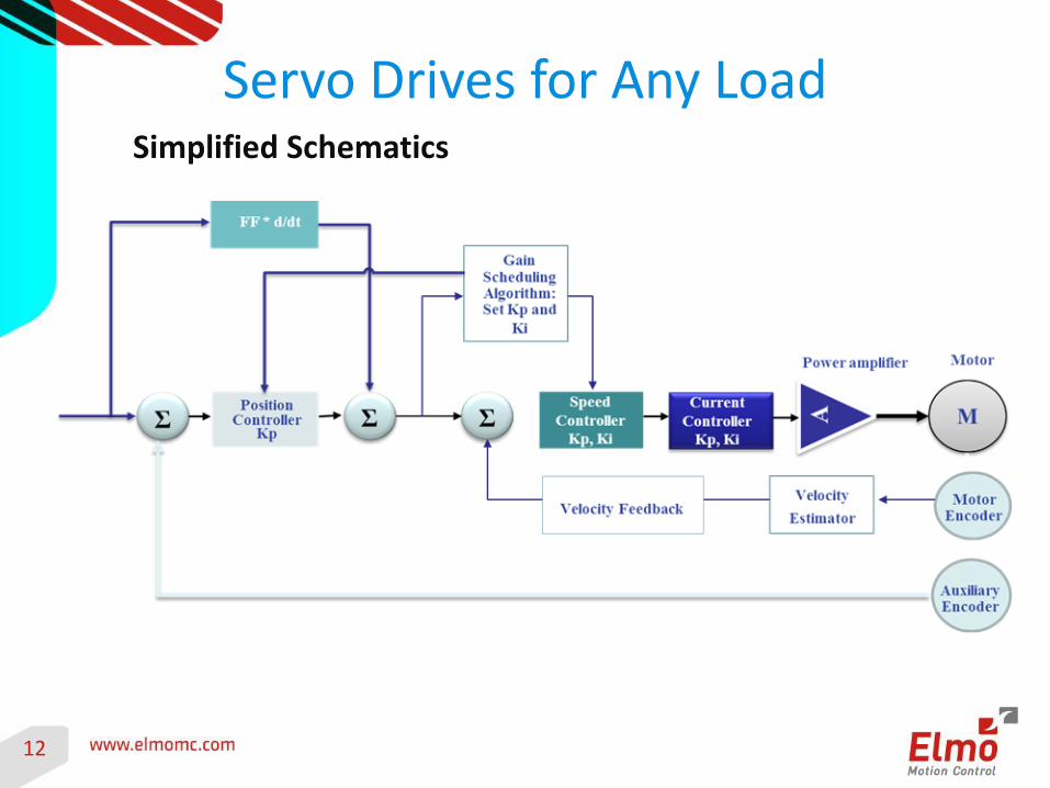
Simplified Schematics


13

The EAS, Supporting Tools

Elmo Application Studio – EAS

EAS is a user-friendly, Windows-based environment

EAS “walks you through” the implementation of any application quickly and simply

EAS brings high-quality results

14

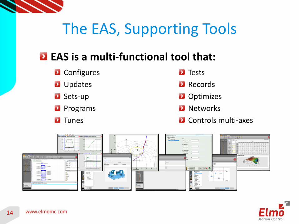
The EAS, Supporting Tools

Configures

Updates

Sets-up

Programs

Tunes

Tests

Records

Optimizes

Networks

Controls multi-axes

EAS is a multi-functional tool that:

15

High-Performance Tuning tool

Fast, easy, efficient and advanced tuning tool

EAS, The Tuning

16

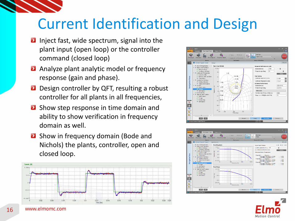
Inject fast, wide spectrum, signal into the plant input (open loop) or the controller command (closed loop)

Analyze plant analytic model or frequency response (gain and phase).

Design controller by QFT, resulting a robust controller for all plants in all frequencies,

Show step response in time domain and ability to show verification in frequency domain as well.

Show in frequency domain (Bode and Nichols) the plants, controller, open and closed loop.

Current Identification and Design

17

Analog sensors are calibrated (for Analog sine/cosine and resolver)

Analog Sensor calibration

18

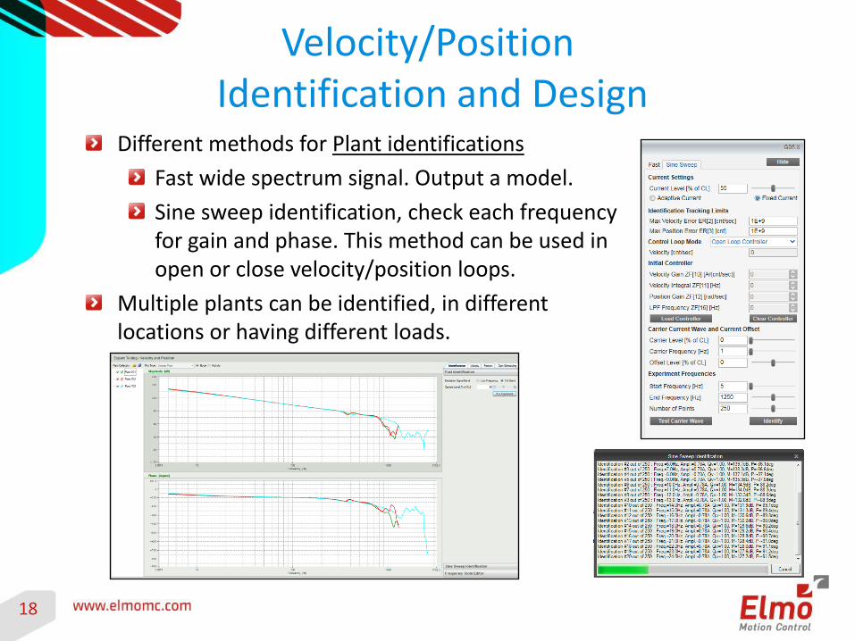
Different methods for Plant identifications

Fast wide spectrum signal. Output a model.

Sine sweep identification, check each frequency for gain and phase. This method can be used in open or close velocity/position loops.

Multiple plants can be identified, in different locations or having different loads.

Velocity/Position Identification and Design

19

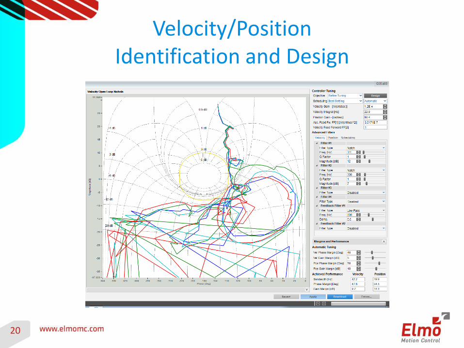
Automatic Controller design method by QFT, resulting in a robust controller for all plants in all frequencies. Few Design Methods Available:

Advanced – Design the PI controller with best LPF and notch filters for the specified Stability margins.

PI Only– Design only the PI controller gains.

PI + LPF – Design the PI controller gains with single LPF @800Hz (for most common systems)

Refine Tuning – Refine the PI controller gains design for any pre defined advanced filters.

Manual design for the advanced control engineer is also possible as an option.


20


21

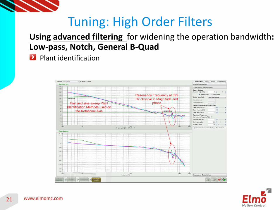
Tuning: High Order Filters Using advanced filtering for widening the operation bandwidth: Low-pass, Notch, General B-Quad

Plant identification

22

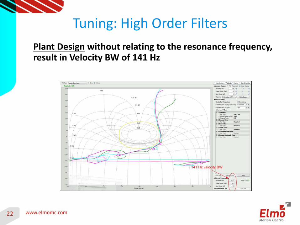
Plant Design without relating to the resonance frequency, result in Velocity BW of 141 Hz

Tuning: High Order Filters

23

Plant Design with Notch Filter at the resonance frequency result in Velocity BW of 165Hz

Results after increasing the velocity loop BW by 15%

Tuning: High Order Filters

24

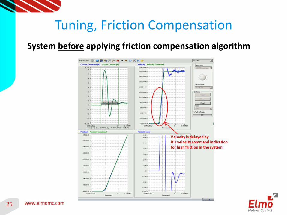
Tuning, Friction Compensation

Different friction compensation methods

Non-linear compensation method to overcome friction by adding an offset command to the integral filter of the velocity loop Using the velocity Gain Scheduling table with high gains in the low speeds In this case, the speed command is used as the index to the scheduled velocity table entry gains

25

System before applying friction compensation algorithm


26

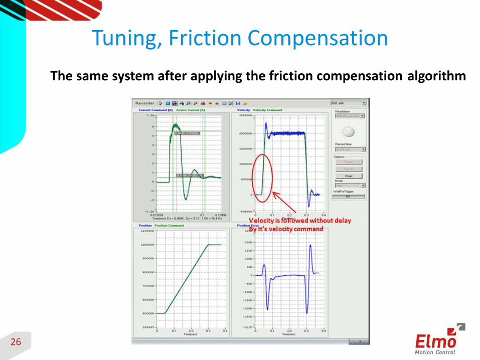
The same system after applying the friction compensation algorithm


27

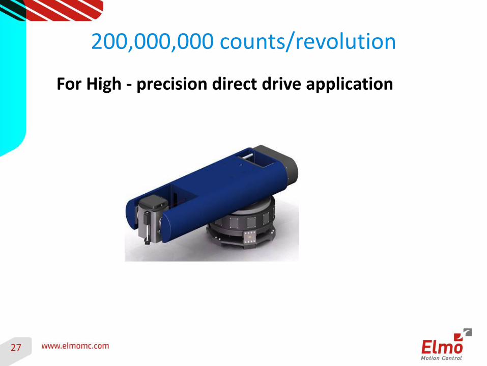
For High - precision direct drive application

200,000,000 counts/revolution

28

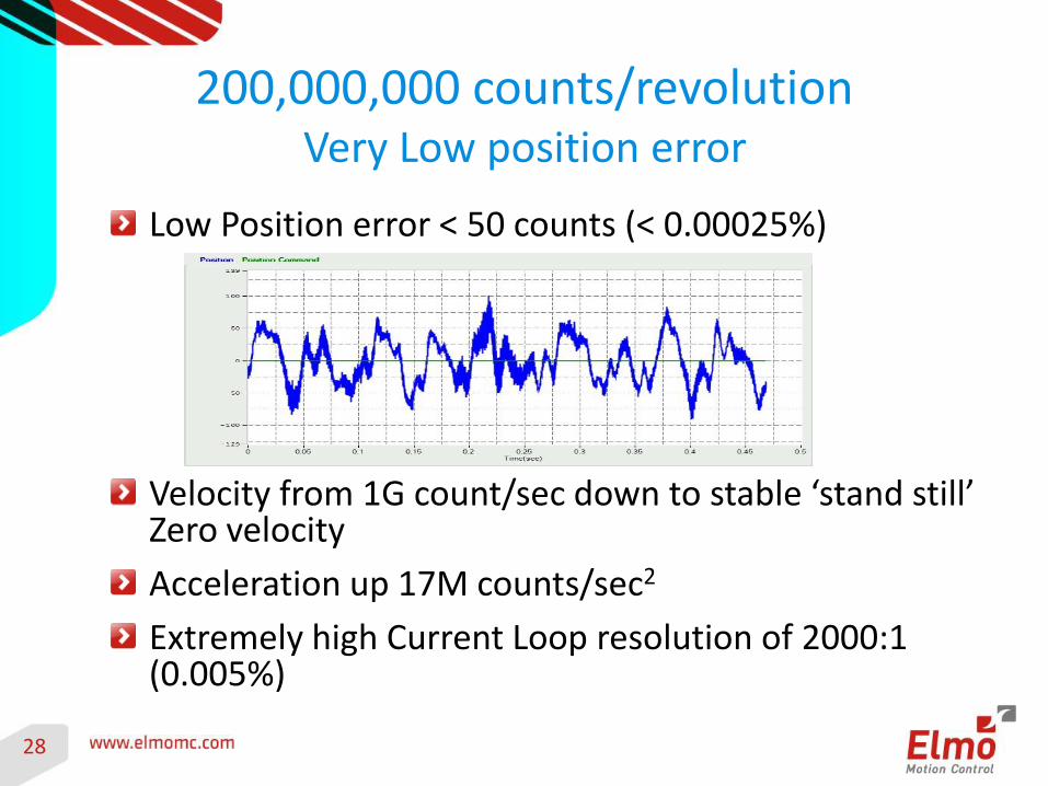
Very Low position error

Low Position error < 50 counts (< 0.00025%)

Velocity from 1G count/sec down to stable ‘stand still’ Zero velocity

Acceleration up 17M counts/sec2

Extremely high Current Loop resolution of 2000:1 (0.005%)

200,000,000 counts/revolution

29

High & Low Speed Requirements

Coping with High/Low speed requirements:

Very Common requirement is very smooth, very precise, “gentle,” low speed and low Torque/Force operation combined with “sharp,” very fast, high acceleration, high deceleration movements. Since Elmo’s servo drives exhibit very high current (Torque/Force) resolution and wide current dynamic range loop, they provide an ideal solution to match perfectly these tough requirements.

200,000,000 count/rev

30

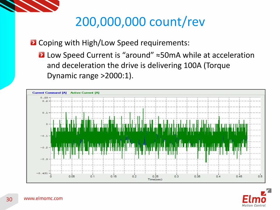
Coping with High/Low Speed requirements:

Low Speed Current is “around” ≈50mA while at acceleration and deceleration the drive is delivering 100A (Torque Dynamic range >2000:1).

200,000,000 count/rev

31

1 Dimension Position Error Correction

Application Example: 1Dimension Error correction for high system accuracy

Using a 23-sided polygon, of which the face angle better than 0,2arc sec (0,00005deg). Without mapping the error is 60arc sec peak-peak After mapping the position error became an error of +/-1arc sec (0.0003deg)

200,000,000 count/rev

32

Elmo Gantry Solution

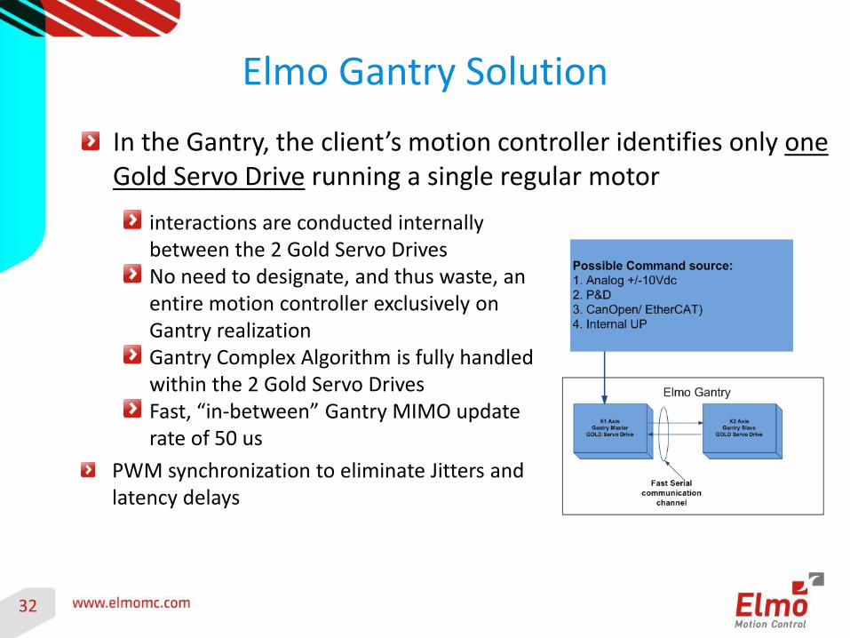
In the Gantry, the client’s motion controller identifies only one Gold Servo Drive running a single regular motor

interactions are conducted internally between the 2 Gold Servo Drives No need to designate, and thus waste, an entire motion controller exclusively on Gantry realization Gantry Complex Algorithm is fully handled within the 2 Gold Servo Drives Fast, “in-between” Gantry MIMO update rate of 50 us

PWM synchronization to eliminate Jitters and latency delays

33

High Demanding Servo Requirements

Application Example: Gantry Stage

Demanding servo control performance using MIMO (Multi Input Multi Output) algorithm implementation

High Resolution 4.88nm resolution, (typically 1.22 ~ 4.88nm , 4096~16384 x interpolation for 20um pitch analog encoder).

Low Jittering in “Stand Still”:

In Gantry axis less than 40nm jitter.

In Cross Axis less than 20nm jitter.

Low Velocity ripple: +- 0.05% at 50mm/sec with 1Khz sample rate.

Fast Settling time : Same result for various moving distance


34

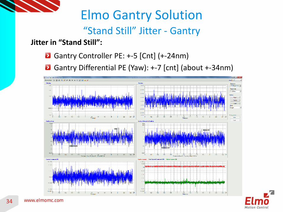
Jitter in “Stand Still”:

Gantry Controller PE: +-5 [Cnt] (+-24nm)

Gantry Differential PE (Yaw): +-7 [cnt] (about +-34nm)

“Stand Still” Jitter - Gantry


35

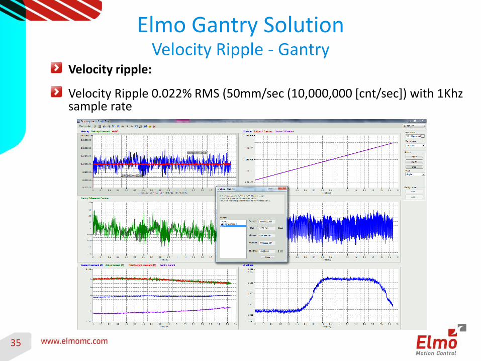
Velocity ripple:

Velocity Ripple 0.022% RMS (50mm/sec (10,000,000 [cnt/sec]) with 1Khz sample rate

Velocity Ripple - Gantry Elmo Gantry Solution

36

Application Example Planar Stage: 1.3mSec PTP axis motion , vector velocity 1.65m/sec, 85Vdc bus voltage, could be chieved using phase advance

High & Low Speed - Planar Elmo Gantry Solution

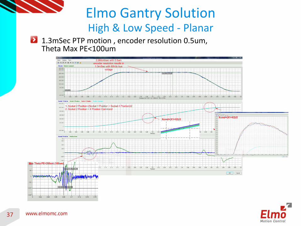
37

1.3mSec PTP motion , encoder resolution 0.5um, Theta Max PE<100um

High & Low Speed - Planar Elmo Gantry Solution

38

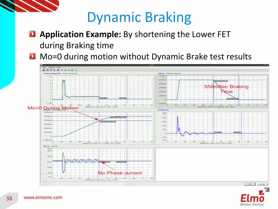
Dynamic Braking Application Example: By shortening the Lower FET during Braking time Mo=0 during motion without Dynamic Brake test results

39

Dynamic Braking Mo=0 during motion With Dynamic Brake implementation

Technology

Servo Drive for Top Performance | ElmoMC