Robust and Tuneable Family of Gossiping Algorithms

Robust and Tuneable Family of Gossiping Algorithms

Vincenzo De Florio

The 20th Euromicro Int.l Conference on Parallel, Distributed and Network-Based ComputingGarching, February 16, 2012

http://www.pats.ua.ac.be/vincenzo.deflorio

Structure

• Introduction – main key words

• Definitions, goals, and assumptions

• Algorithms and tuning algorithms

• Conclusions and lessons learned

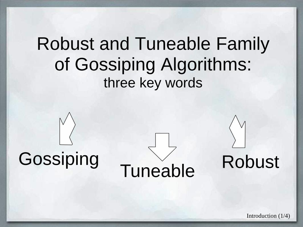
Robust and Tuneable Family of Gossiping Algorithms:

three key words

GossipingTuneable

Robust

Introduction (1/4)

Gossiping

• All-to-all pairwise IPC• Every member of a set

communicates aprivate value to allother members

• Useful e.g. inrestoring organs,distributed consensus,interactive consistency...

Introduction (2/4)

Tuneable

• An example of a tuneable algorithmo An application layer "knob"

to select certain behaviours rather than others

o Explicit knob:one we are aware ofand know how to steer

o (As opposed to a hidden knob:one that we don't know it exists

nor how to use!)

Introduction (3/4)

Robust

• A robust knob: one that allows • persistence of certain behaviours despite changes in the

context• to match fundamental assumptions regarding the

environment in which the system operates [Jen04]

• An in particular, to match dynamically changing assumptions: robustness throughout system evolution Resilience

Introduction (4/4)

Definitions

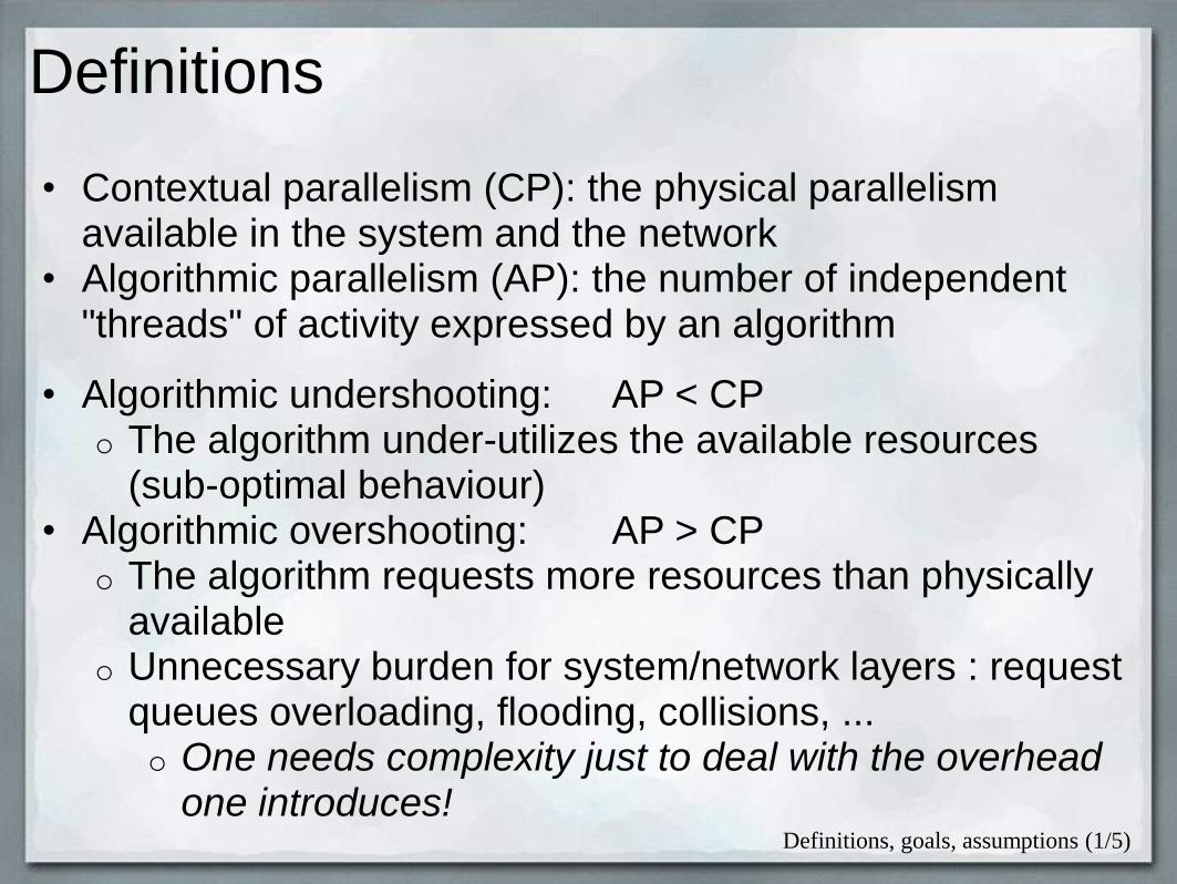
• Contextual parallelism (CP): the physical parallelism available in the system and the network

• Algorithmic parallelism (AP): the number of independent "threads" of activity expressed by an algorithm

• Algorithmic undershooting: AP < CPo The algorithm under-utilizes the available resources

(sub-optimal behaviour)• Algorithmic overshooting: AP > CP

o The algorithm requests more resources than physically available

o Unnecessary burden for system/network layers : request queues overloading, flooding, collisions, ...o One needs complexity just to deal with the overhead

one introduces!Definitions, goals, assumptions (1/5)

Main design goal

• Dynamically robust tuning:o Optimal match between AP and CP over timeo Dynamic avoidance of shortcoming or excess

of algorithmic parallelism

Definitions, goals, assumptions (2/5)

Assumptions

• N + 1 processors (N>1)• Full-duplex point-to-point communication lines• Communication: synchronous and blocking• Processors are uniquely identified by

integer labels ∈ IN = {0, ..., N}

• Each processor pi owns some local data vi

• Each processor requires the other processors’ local data and then executes some algorithm (e.g. voting)

• Events occur by discrete time steps


State templates

• WR state. A process is waiting for the arrival of a message from some processor.• Lasts zero or more time steps

• R state. Process i receiving at time t a message from process j is said to be in state Rj . This is represented as i Rt j• Lasts one step

• WS state. Process i waiting to send process j its message is said to be in state WSj . • Lasts zero or more time steps

• S state. Process i is at time t in state Sj when it is sending a message to process j. This is represented as i St j• Lasts one time step


Index permutation

• Process i owns an index permutation, i.e. an array whose members are permutations of

{ 0, …, i -1, i +1, …, N }

• P = { P1, …, PN } is used to represent the index

permutation


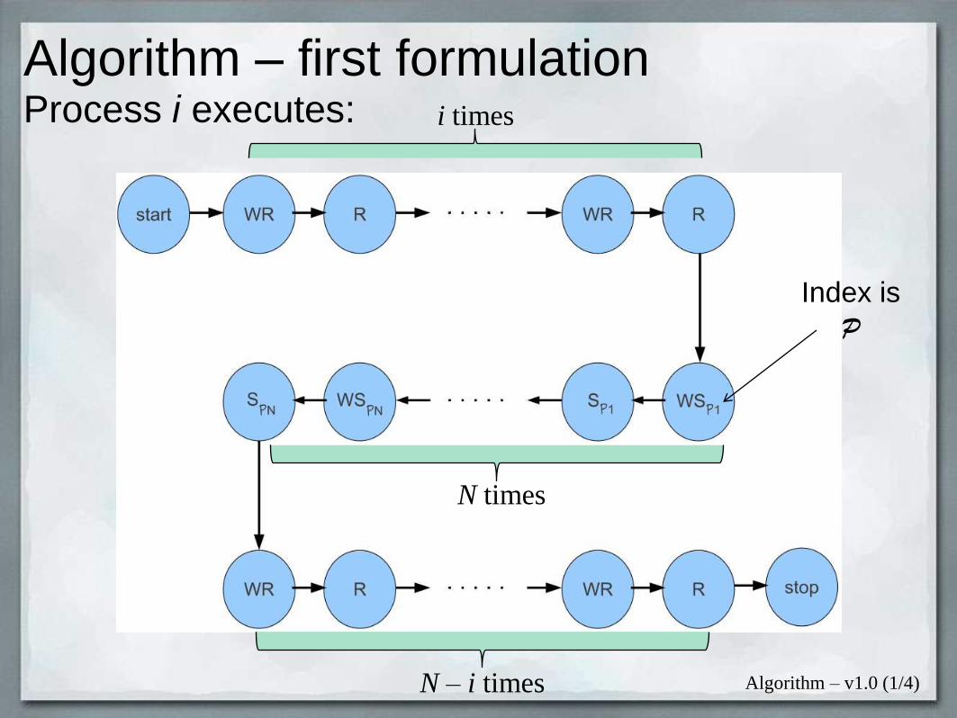
Algorithm – first formulationProcess i executes:

Algorithm – v1.0 (1/4)

i times

N times

N – i times

Index is

P

Properties

• Whatever the index permutation, the algorithm does work• In [DeBl06] we analyzed the efficiency of the algorithm

when P takes a given structure

• In particular,

• When P is the identity permutation :

P = { 0, ..., i - 1, i + 1, ..., N }

• When P is the pipelined permutation :

P = { i + 1, ..., N, 0, ..., i - 1 }


Identity permutation, N = 5

• AP = about 2.31• Asymptotic value of AP(N) = 8/3


• Table = transcript of states• e.g. Proc. 3 at step 8 receives from proc 1 = 3 R8 1• Arrow-to-the-left = WR; arrow-to-the-right = WS

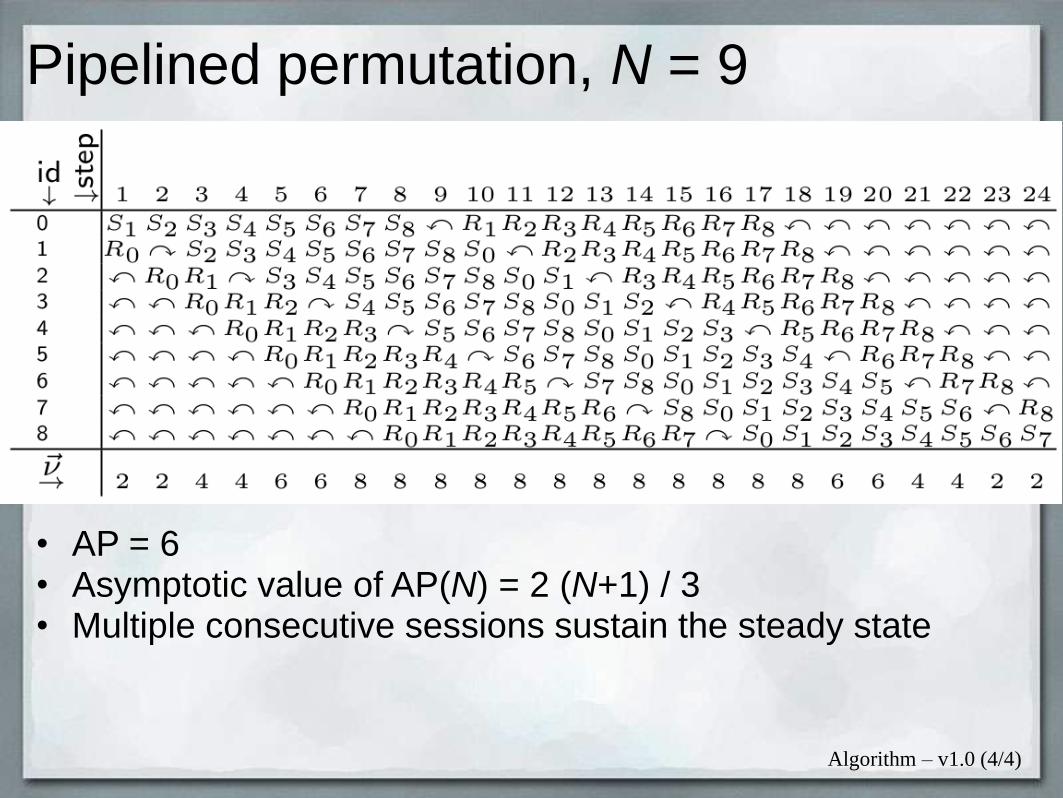
Pipelined permutation, N = 9

• AP = 6• Asymptotic value of AP(N) = 2 (N+1) / 3• Multiple consecutive sessions sustain the steady state


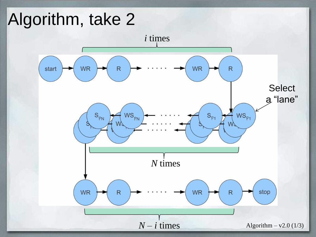
Algorithm, take 2


i times

N times

N – i times

Select

a “lane”

Algorithm, v2.0

• In what follows we consider just two types of “lanes”: either with identity or with pipelined permutations

• We assign H% to pipelined and (100-H)% to identity• (H for “Hybrid”)

• Results: • AP(identity) ≤ AP(H) ≤ AP(pipelined)• AP(H) increases with H


Algorithm, v2.0


Observations

This paves the way to context aware adaptation:

Observations (1/2)

A MAPE adaptation loop:

M: Estimate CP(now)A: assess how AP(now) matches CP(now):

Case of overshooting? Case of undershooting?P: If *-shooting, select H% so as to make

AP(now') “closer” to CP(now)E: use Algorithm v2.0 with selected H%

so as to guarantee our design goals (dynamic robust tuning)

Observation

• Instead of running Alg. v2.0 to compute AP values, we may use offline-computed values:

M(N,h) = AP• A look-up table storing the algorithmic parallelism

corresponding to CP(t) = N and H% = h

Observations (2/2)

Adaptation algorithms

• Algorithm “Tune AP after CP”, v.1Input: CP(t), N, M( (N, h) → AP )Output: H% best matching CP(now())

begincp sense(CP(now()) // cp is now the current

// physical parallelismH min{h | M(N,h) >= cp} // H: sample

// corresponding to// the supremum

return Hend .

Robust tuning (1/4)

• Observation: A “growing” look-up table would allow to keep track of past decisions

• growMap (M, new ( (N, h) → AP ) )

Adaptation algorithms

• Algorithm “Tune AP after CP”, v.2Input: CP(t), N, M( (N, h) → AP )Output: H% best matching CP(now())

begincp sense(CP(now())sup min {h | M(N,h) >= cp}if M(N,sup) == cp then return sup end-if// M(N,sup) > cpinf max {h | M(N,h) < sup}newH ( M(N,sup) - M(N,inf) ) / 2ap compute(newH) // executes a run

// and returns the APgrowMap (M, (N,newH) ap )return newH

end . Robust tuning (2/4)

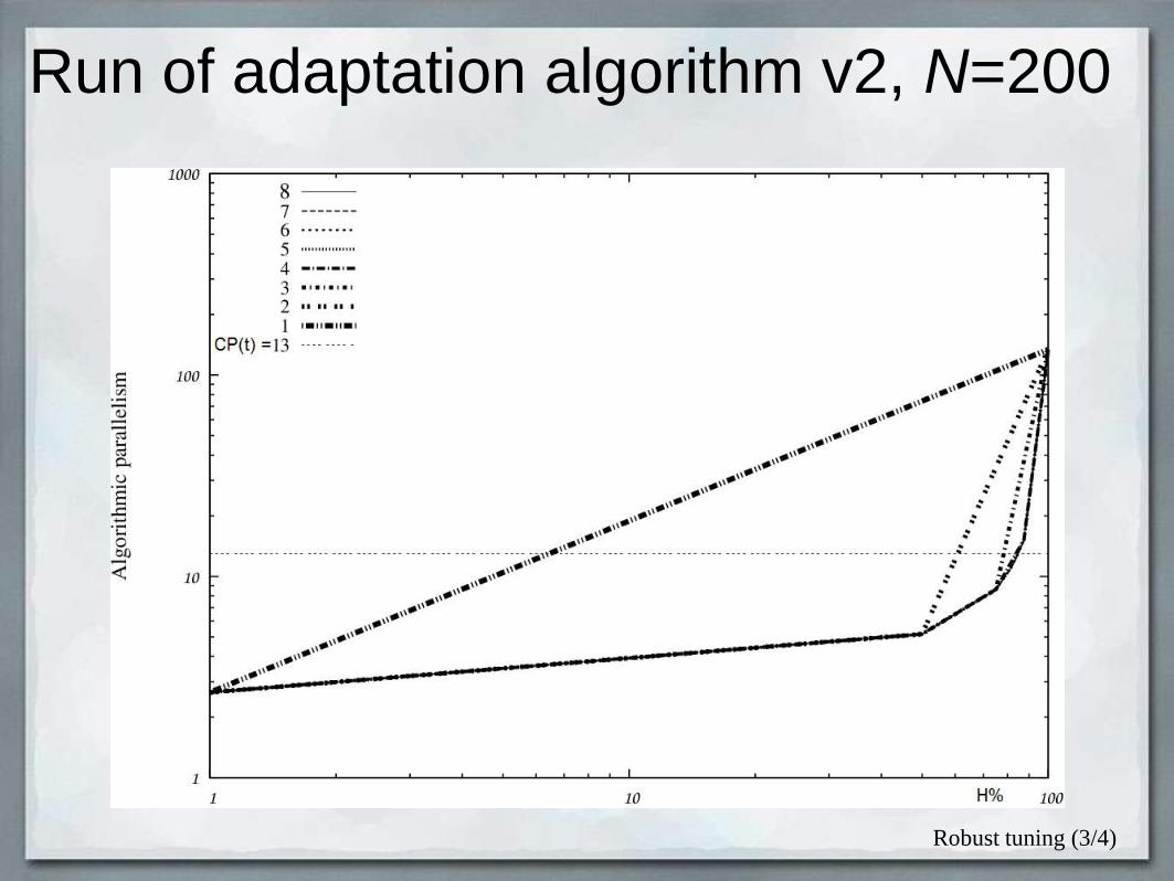
Run of adaptation algorithm v2, N=200

Robust tuning (3/4)

A run of algorithm v2

1. 1 2.653465100 134

2. 1 2.65346550 5.170751100 134

3. 1 2.65346550 5.17075175 8.621984100 134

4. 1 2.65346550 5.17075175 8.62198487.5 15.241706100 134

5. 1 2.65346550 5.17075175 8.62198481.5 11.01822787.5 15.241706100 134

6. 1 2.65346550 5.17075175 8.62198481.5 11.01822784.5 12.75380787.5 15.241706100 134

7. 1 2.65346550 5.17075175 8.62198481.5 11.01822784.5 12.75380786 13.87642487.5 15.241706100 134

8. 1 2.65346550 5.17075175 8.62198481.5 11.01822784.5 12.75380785 13.10513486 13.87642487.5 15.241706100 134

Robust tuning (4/4)

• An application-layer “knob” to tune algorithmic parallelism• A knob that allows us to achieve robustness throughout

system evolution (ability to match dynamically changing assumptions) = resilience

Conclusions & Lessons Learned

Conclusions (1/3)

• When performing e.g. cross-layer adaptation, one deals with many intertwined VMs• Application layer, application server layer, OS, the

network layers, the HW...Stigmergy everywhere!

• These VMs may appear to the adaptation engineer as• White boxes: known robust knobs we are aware of• Grey boxes: known knobs we are partially aware of• Black boxes: hidden knobs

• Excluding the application layer (the algorithm) locks in to inefficiency or non-robustnessWe need to expose the algorithmic knobs!Sort of an “End-to-end Argument” in system evolution [SaRC84]

Conclusions & Lessons Learned

Conclusions (2/3)

[SaRC84] Saltzer, Reed & Clark, “End-to-End Arguments in System Design,” ACM Trans. on Computer Systems 2:4 (1984)

[Jen04] E. Jen, “Stable or robust? What’s the difference?” InE. Jen, editor, Robust Design: A repertoire ofbiological, ecological, and engineering case studies,Oxford University Press, 2004.

[DeBl06] V. De Florio & C. Blondia, “The Algorithm of Pipelined Gossiping,” Journal of Systems Architecture 52:4, 2006

Main sources

Conclusions (3/3)

Systems robust throughout their evolution:

More info: http://www.igi-global.com/ijaras

Technology

Robust and Tuneable Family of Gossiping Algorithms