Presented by Muhammad Safdar

Outline Introduction of A Study Area Interpolation Spatial Interpolation & Methods

- Spline- Inverse Distance Weighting(IDW)- Kriging

Methodology- Study site

Data Collection Process & Representation Tools Results Conclusion

Introduction of A Study Area

In a pilot Area of Caracas, Venezuela

Frequency range of 100 kHz to 6 GHz

Taking 35 samples per second during a 6 minutes , 206 measurements points

Data points spaced approximately 100m from each other is fixed over the 2.64km2 pilot area

Interpolation?

Interpolation is a method of constructing

new data points within the range of a discrete set of known data points.

Spatial Interpolation?

Interpolation predicts values for cells in a raster from a limited number of sample data points. It can be used to predict unknown values for any geographic point data: elevation, rainfall, chemical concentrations, noise levels, and so on.

Spatial Interpolation Methods

1.Spline

method estimates values using a mathematical function

that minimizes the total surface curvature, resulting in a

smooth surface that passes exactly through the sampled points

2.Inverse Distance Weighting(IDW)

• is based on the assumption that the nearby values contribute more to the interpolated values than distant observations.

3. Kriging

depends on spatial and statistical relationships to

calculate the surface.

MethodologyStudy Site.

The measurements were taken in a pilot zone of Caracas,

Venezuela(Figure 1)with an approximate area of 2.64km2,

which represents 0.609% of the total geographical area of

the Caracas. A total of 206 measurements points, were

selected over the pilot zone. This area is characterized by

a dynamic economic-business activity which is evident

given the presence of shopping centers, office buildings of

the national telephone operators and other

telecommunications companies. On the other hand, this

area also boasts a large number of hospitals and schools,

which is of interest to know the impact of electromagnetic fields.

Data Collection Process

Time considerations : Measurements were taken over a period of 30 days, from

February 15th to March 15th of 2010. Measurements were performed only on working days (from Mondays to Fridays).Each measurement was taken between 8:00 am and 5:00 pm.

Geographical considerations:

each measurement point geographical coordinates were taken using a GPS navigation unit.

Measurement considerations:

Data Process and Representation Tools

Two informatics tools

1: GvSIG 1.9

2: Past 2.02. GvSIG is a Geographic Information System (GIS)

Both free software tools distributed under the GNU/GPL license.

ResultsMagnitude. (a) IDW, (b) SPLINES, (c) KRIGING.

.Table 1. Results of the measures of ¯t applied to the interpolation methods.

MEASURES MAE MSE D (V/m)

Max Error Min Error

OF FIT (V/m) (V/m)2 (V/m) (V/m)

IDW 0.17 0.05 1.01 0.55 0.008

KRINGING 0.74 0.73 3.81 1.66 0.111

SPLINE 0.89 1.11 4.71 1.98 0.034

.

Averag

eM

ag

nit

ud

e(V

/m)

Estim

ate

d E

lectr

ic F

ield

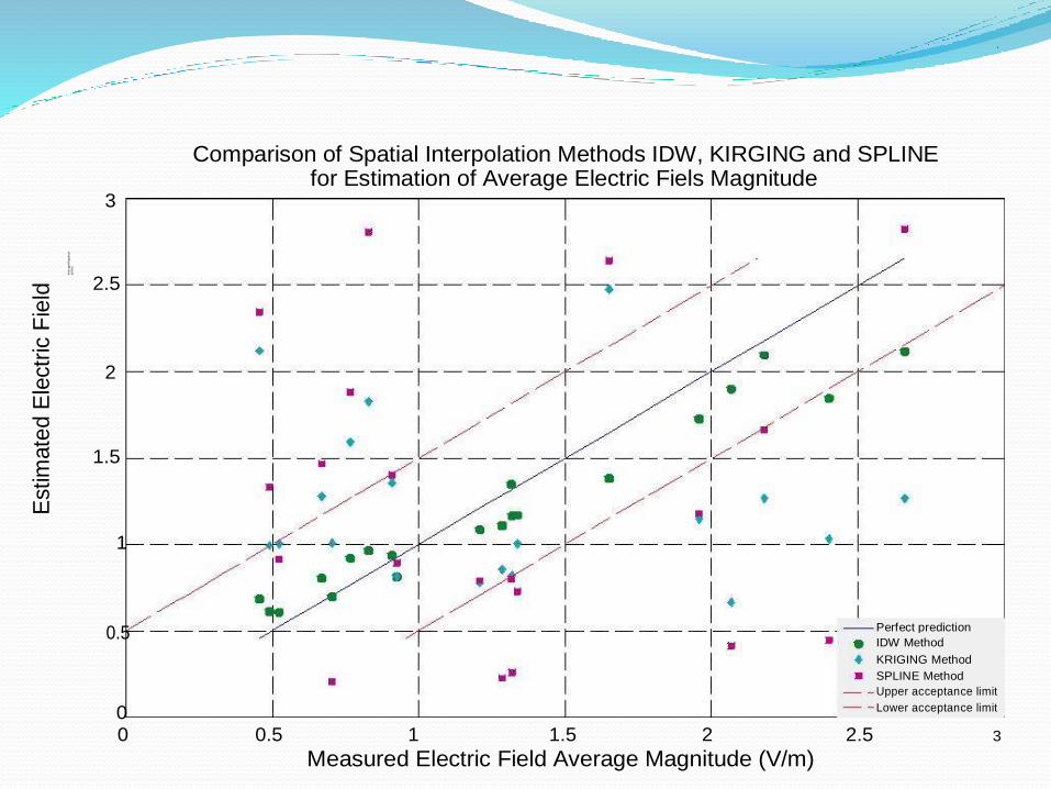
Comparison of Spatial Interpolation Methods IDW, KIRGING and SPLINE for Estimation of Average Electric Fiels Magnitude

3 2.5

2 1.5

1

0.5 Perfect prediction

IDW Method

KRIGING Method

SPLINE Method

Upper acceptance limit

0 Lower acceptance limit

0 0.5 1 1.5 2 2.5 3 Measured Electric Field Average Magnitude (V/m)

.

.

Conclusion

This study has shown that IDW interpolation

method is most likely to produce the best

estimation of a continuous surface of the

average magnitude of electric field intensity.

The IDW method exactness was superior to

the one shown by the SPLINES and

KRIGING techniques.

Thanks

Questions?