PTE 588: SMART OILFIELD DATA MINING

FALL 2015

Topic: Oil and Gas Production Forecasting

Using Data Mining Techniques

Project Report

Team (4) Members:

Sultan Attiah

Long Vo

Walter Morales

Abhishek Ajith

Page 1 of 30

Contents

1. Objective And Solution Of The Project

2. Background On Ventura Oilfield

Ventura Oilfield

Geology

Production In Ventura County

Why There Are Less Injection Wells In Ventura County

3. Data Mining Process

Data Preparation

Data Surveying

Data Modeling

4. Conclusion

5. Implementation Of This Project

6. References

Page 2 of 30

Objective:

The objective of the project is to create a model of a reservoir using the data mining technique

by analyzing and interpreting field data. Moreover, characterize the reservoir after matching

the production from existing wells to find the best drilling spots, predict future production of

new wells and identify the best well type associated with the location.

Data Mining Process

For the purpose of this project we have selected the Ventura Oil Field; the first step in the data

mining process was the data preparation step, this consisted of gathering the data from the

DOGGR web page and cleaning and preprocessing the data. The data was plotted and mapped

to detect the relationship among attributes. Finally, the modeling step was performed. A detail

description of all these three steps will be described in this section.

1) Data Preparation Process:

Data gathering:

o Download the data

o Construct master database to link all downloaded databases together and

connect them by using an SQL script in order to query the data

o Eliminate all duplicate and “bad data”; replace all null data by zeros to prevent

problem when aggregating the data (for example when calculating cumulative

production)

o Review the structure of the data and make sure that “irrelevant” data is kept out

of the analysis

2) Data Surveying Process:

Calculate cumulative plots:

o Construct cumulative production plots for the entire field on well by well basis

o Calculate well counts based in oil active wells

Data Normalization:

o Clean all initial production recorded as zero from the production table for all

wells.

o Create a VBA macro in order to normalize the production time per month

Page 3 of 30

Data Classification:

o Calculate ratios (BOPD, BWPD, BGPD), peak oil (BOPD) and the time that the

well takes to reach its peak production or ramp time(Normalized time in

months)

o Generate statistics and distribution plots in order to classify all wells based in the

calculated properties.

o Classify the wells base in the calculated properties

Data Visualization:

o Use the previous classification to generate maps and normalized cumulative

production in order to investigate the relationships between several attributes

3) Data Modeling Process:

Data Preprocessing:

o Filter non-essential attributes.

o Identify nominal and numeric attribute types

o Identify the class attribute

o Normalize all numeric attribute to have the same scaling

Sampling:

o Divide dataset into training and testing set using Weka supervised resample filter

80% used for training set

20% used for testing set

Build cluster model from Simple K-Means:

o Create 3 sub model to test for overfitting:

3 cluster

5 cluster

10 cluster

Compare training set output cluster with testing set output cluster:

o Determine error

o Determine validity of sample set

Page 4 of 30

Evaluate and extract knowledge from cluster results:

o Location

o Production

o Ramp time

o Peak production

o Well type

Form conclusion and advise on well type, location, and productivity

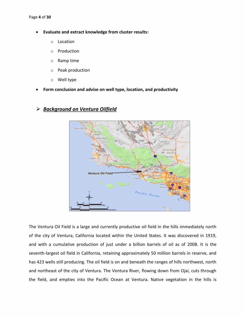
Background on Ventura Oilfield

The Ventura Oil Field is a large and currently productive oil field in the hills immediately north

of the city of Ventura, California located within the United States. It was discovered in 1919,

and with a cumulative production of just under a billion barrels of oil as of 2008. It is the

seventh-largest oil field in California, retaining approximately 50 million barrels in reserve, and

has 423 wells still producing. The oil field is on and beneath the ranges of hills northwest, north

and northeast of the city of Ventura. The Ventura River, flowing down from Ojai, cuts through

the field, and empties into the Pacific Ocean at Ventura. Native vegetation in the hills is

Page 5 of 30

predominantly chaparral and coastal sage scrub, and riparian woodland is found along the

course of the Ventura River. The terrain on the hills is steep, and the roads to well pads, tanks,

and other infrastructures make numerous switchbacks. Most of the field is hidden from view

from the city because of the first steep range of hills. The oil field is one of several following the

east-west trend of the Transverse Ranges at this point: to the west are the San Miguelito Oil

Field and the Rincon Oil Field, and to the east, across the Santa Clara River valley, the large

South Mountain Oil Field adjacent to Santa Paula and the smaller Saticoy Oil Field along the

Santa Clara River east of Saticoy. To the north are the smaller Ojai and Santa Paula fields. Total

productive area of the field, projected to the surface, encompasses 3,410 acres (13.8 km2).

Geology:

In the Ventura field, the large-scale structural feature responsible for petroleum accumulation

is the Ventura Anticline, an east-west trending geologic structure 16 miles (26 km) long, visible

in the numerous rock outcrops in the rugged topography of the area. This anticline dips steeply

on both sides, with the dip angle ranging from 30 to 60 degrees, resulting in a series of rock

beds resembling a long house with a gabled roof, under which oil and gas collect in abundance.

The underlying Monterey Formation is presumed to be the source of the oil accumulations in

the Ventura field, as well as the other two fields in the same geologic trend. The Monterey

Formation is rich in organic matter, averaging 3-5 percent but reaching 23 percent in some

area. Oil gravity and sulfur content are similar in all pools in the field, with an API gravity of 29-

30 and approximately 1 percent sulfur by weight.

Production In Ventura County:

Occidental, which is one of the largest operators in Ventura County through Vintage Production

California LLC, stated it added wells in existing fields, explored in areas slightly outside of known

reserves and brought old wells back into use in California, resulting in 124 new wells and 388

wells being worked over. “Improved oil recovery increases the volume of oil pulled from a

reservoir, while enhanced oil recovery techniques help Occidental continue extracting oil from

a reservoir after primary and secondary recovery methods have been used” as stated by

Occidental spokesperson which outlines their objective. As of 2011 the number of active wells

in Ventura stands at 1708 and the oil produced in barrels is estimated to be around 8,308,059.

Page 6 of 30

Because of this production boom Vintage Petroleum, a subsidiary of Occidental Petroleum, has

entered into 192 lease agreements over the past six months in deals involving at least 9,000

acres. Since acquiring properties in Ventura County in 2006, Vintage Production California has

reworked field infrastructure to support and expand existing projects and develop new

opportunities for oil recovery. In the 1960's, the first serious exploration of submerged lands

was undertaken, which led to the discovery of two large oil fields off the Coast of Santa Barbara

County. Subsequently, Ventura County oil exploration efforts were then concentrated on

offshore fields and operators began to explore new, more efficient methods of oil production.

(e.g.: Fracking & EOR Techniques).

Why Are There Less Injection Wells in Ventura County:

Injection wells can be used for enhanced oil field recovery processes like a water flood, steam

flood, and cyclic steam injection, as well as oilfield wastewater disposal. These are called Class II

injection wells which are a special label for injection well sand they are regulated by DOGGR

through an agreement with the EPA. Ventura County doesn’t have many Injection Wells due to

the fact it has several environmental regulations and bans imposed over alleged use of harmful

fracking fluids which has seeped into nearby deep water aquifers and contaminated

groundwater. (The Anterra site – a commercial Class II Injection Well).

The real environmental issue surrounding hydraulic fracturing is not the loss of local vegetation,

but the effects this process has on local groundwater. So Ventura County updated its oil

application process to require new drilling proposals involving fracking or acidizing to provide

detailed information, including the source and amount of freshwater used, and disposal

methods for frac flow back and other wastewater.(which is a hindrance).

Another reason is after a CalTech Study linking induced seismicity with fracking gained traction,

many councils have blindly presumed the correlation between minor earthquakes and hydraulic

fracturing. The Environmental Protection Agency(EPA) has put the California State oil and gas

regulators: the Division of Oil, Gas and Geothermal Resources (DOGGR) on notice regarding

“serious deficiencies” in the way it has been overseeing the permitting of underground

injection wells, which may have compromised groundwater resources. Underground injection

Page 7 of 30

disposal wells are used by oil-field operators to dispose of all sorts of oil-field waste, from

drilling mud to flow back fluids from hydraulic fracturing — it all can be injected into these

wells. The rules about these injection wells are based on protections created by the Federal

Safe Drinking Water Act, which is meant to ensure that aquifers with the potential to be used

for drinking water or irrigation are protected. The EPA’s definition of an underground source of

drinking water is any aquifer with less than 10,000 parts per million (ppm) total dissolved solids

(TDS). The EPA has determined that injection wells in Ventura County have operated in aquifers

with less than 10,000 ppm, less than 3,000 ppm and aquifers with unknown amounts of TDS,

making further testing necessary. An aquifer can also be found exempt if it is determined that it

is likely to never be used as a drinking water source.

Data Mining Process (in details):

1. Data Preparation

This data was obtained from the DOGGR web page and downloaded from the following

webpage (FTP Server): ftp://ftp.consrv.ca.gov/pub/oil/new_database_format/

The following is a view of the FTP site that contains the data:

Figure 1: View of the production databases available in the DOGGR webpage.

Page 8 of 30

Please note the following regarding the data found in the DOGGR webpage.

a. We focused in all production and injection data available for the Ventura Oil Field. The

DOGGR only has electronic databases of oil production for all wells in California starting

in 1977.

b. The data is available in Zip format; therefore after downloading the data, all databases

were decompressed.

c. All databases containing production and completion data for all wells in California

were successfully downloaded.

A database linking of other databases was constructed using MS ACCESS and UNION SQL

statements were to link them together, then wells from the Ventura Oil Field were identified

and their associated oil, water, and gas production was queried. A total of 2475 oil producers

were identified since 1977 until August 2015. From the 2475 wells located in the field, a total

1063 wells have production information in the DOGGR databases.

All other data, from 1977 and older is kept in pdf files and it is available in the DOGGR files, we

didn’t considered this information and only used the information that was available in digital

format (From 1977 until 2015)

2. Data Structure

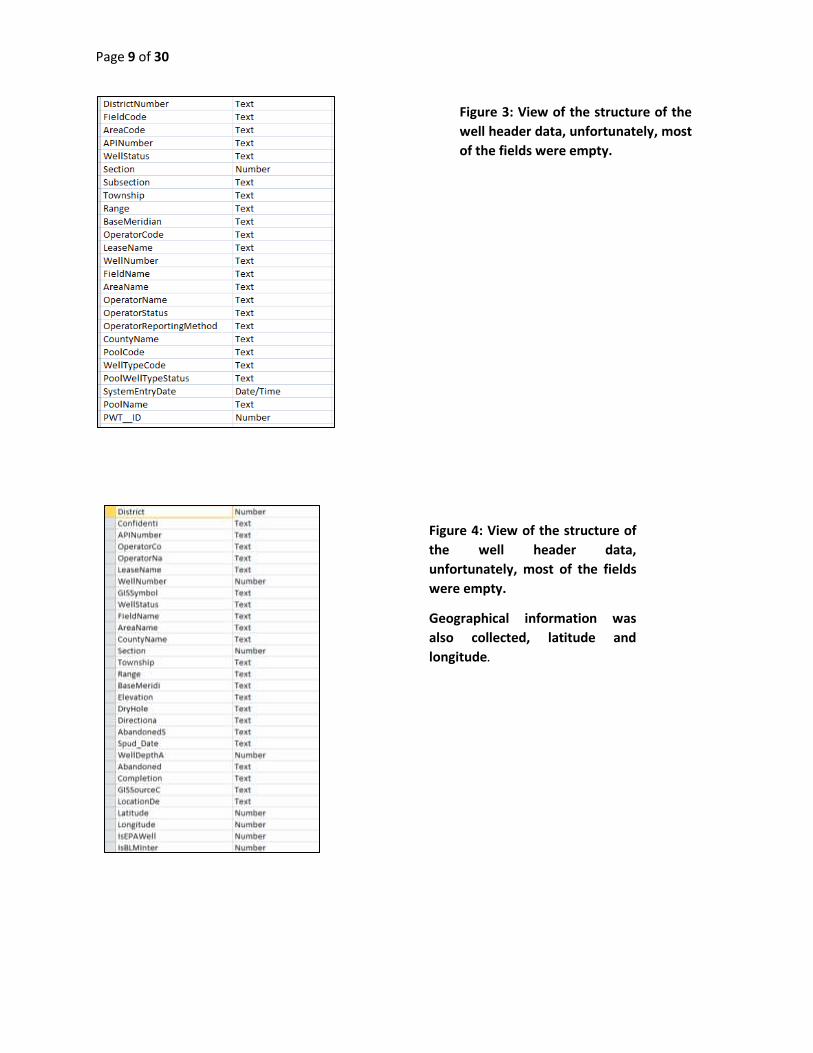
Structure of the well header data collected for all wells in the Ventura Oil Field:

Figure 2: All DOGGR databases after being downloaded and extracted

Page 9 of 30

Figure 3: View of the structure of the

well header data, unfortunately, most

of the fields were empty.

Figure 4: View of the structure of

the well header data,

unfortunately, most of the fields

were empty.

Geographical information was

also collected, latitude and

longitude.

Page 10 of 30

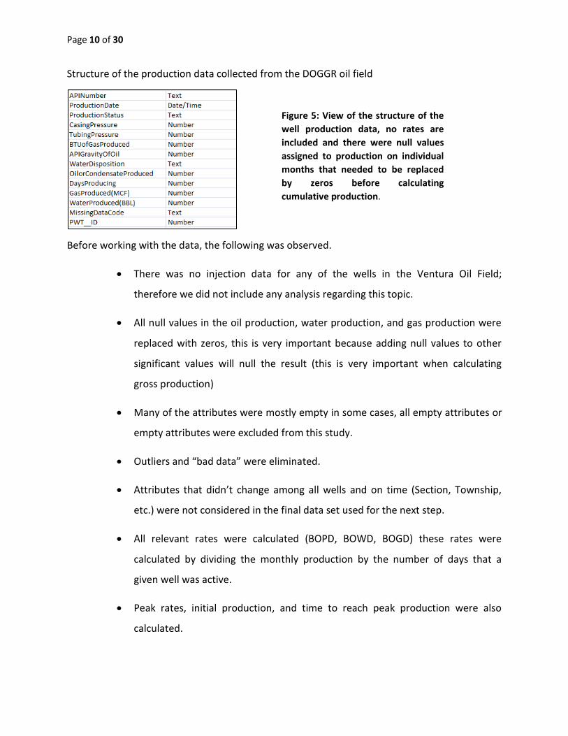
Structure of the production data collected from the DOGGR oil field

Before working with the data, the following was observed.

There was no injection data for any of the wells in the Ventura Oil Field;

therefore we did not include any analysis regarding this topic.

All null values in the oil production, water production, and gas production were

replaced with zeros, this is very important because adding null values to other

significant values will null the result (this is very important when calculating

gross production)

Many of the attributes were mostly empty in some cases, all empty attributes or

empty attributes were excluded from this study.

Outliers and “bad data” were eliminated.

Attributes that didn’t change among all wells and on time (Section, Township,

etc.) were not considered in the final data set used for the next step.

All relevant rates were calculated (BOPD, BOWD, BOGD) these rates were

calculated by dividing the monthly production by the number of days that a

given well was active.

Peak rates, initial production, and time to reach peak production were also

calculated.

Figure 5: View of the structure of the

well production data, no rates are

included and there were null values

assigned to production on individual

months that needed to be replaced

by zeros before calculating

cumulative production.

Page 11 of 30

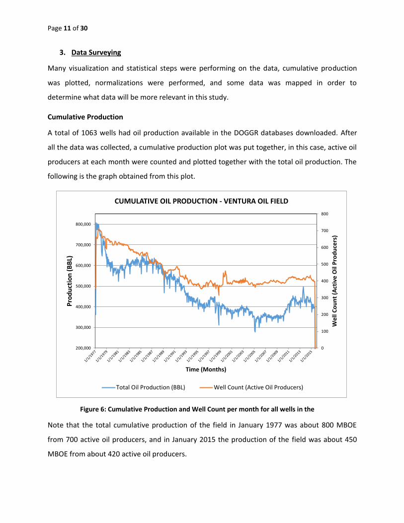
3. Data Surveying

Many visualization and statistical steps were performing on the data, cumulative production

was plotted, normalizations were performed, and some data was mapped in order to

determine what data will be more relevant in this study.

Cumulative Production

A total of 1063 wells had oil production available in the DOGGR databases downloaded. After

all the data was collected, a cumulative production plot was put together, in this case, active oil

producers at each month were counted and plotted together with the total oil production. The

following is the graph obtained from this plot.

Note that the total cumulative production of the field in January 1977 was about 800 MBOE

from 700 active oil producers, and in January 2015 the production of the field was about 450

MBOE from about 420 active oil producers.

0

100

200

300

400

500

600

700

800

200,000

300,000

400,000

500,000

600,000

700,000

800,000

We

ll C

ou

nt

(Act

ive

Oil

Pro

du

cers

)

Pro

du

ctio

n (

BB

L)

Time (Months)

CUMULATIVE OIL PRODUCTION - VENTURA OIL FIELD

Total Oil Production (BBL) Well Count (Active Oil Producers)

Figure 6: Cumulative Production and Well Count per month for all wells in the

Ventura oil Filed

Page 12 of 30

There is an incremental production starting at the end of 2011, this is due to the massive

introduction of horizontal wells.

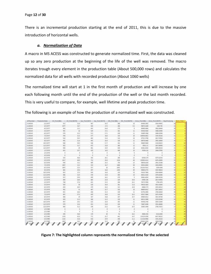
a. Normalization of Data

A macro in MS ACESS was constructed to generate normalized time. First, the data was cleaned

up so any zero production at the beginning of the life of the well was removed. The macro

iterates trough every element in the production table (About 500,000 rows) and calculates the

normalized data for all wells with recorded production (About 1060 wells)

The normalized time will start at 1 in the first month of production and will increase by one

each following month until the end of the production of the well or the last month recorded.

This is very useful to compare, for example, well lifetime and peak production time.

The following is an example of how the production of a normalized well was constructed.

Figure 7: The highlighted column represents the normalized time for the selected

well.

Page 13 of 30

b. Classification of Data

Some statistics was performed in order to further classify this data based on relevant

characteristics.

Total Cumulative Oil Production (BBL)

This is the total cumulative production of a well since the beginning of its production until the

well was abandoned or the last month with the record. The total cumulative production

indicates the production of the well in its entire life. Usually, it is important to identify what

drives high production wells.

The data was plotted and we clearly see that most of the wells have low cumulative

production. This happens because many of the new wells haven’t produced enough time to me,

therefore low cumulative production is expected.

Figure 8: Distribution of the cumulative oi production (BBL) of al wells in the Ventura Oil

Field

Page 14 of 30

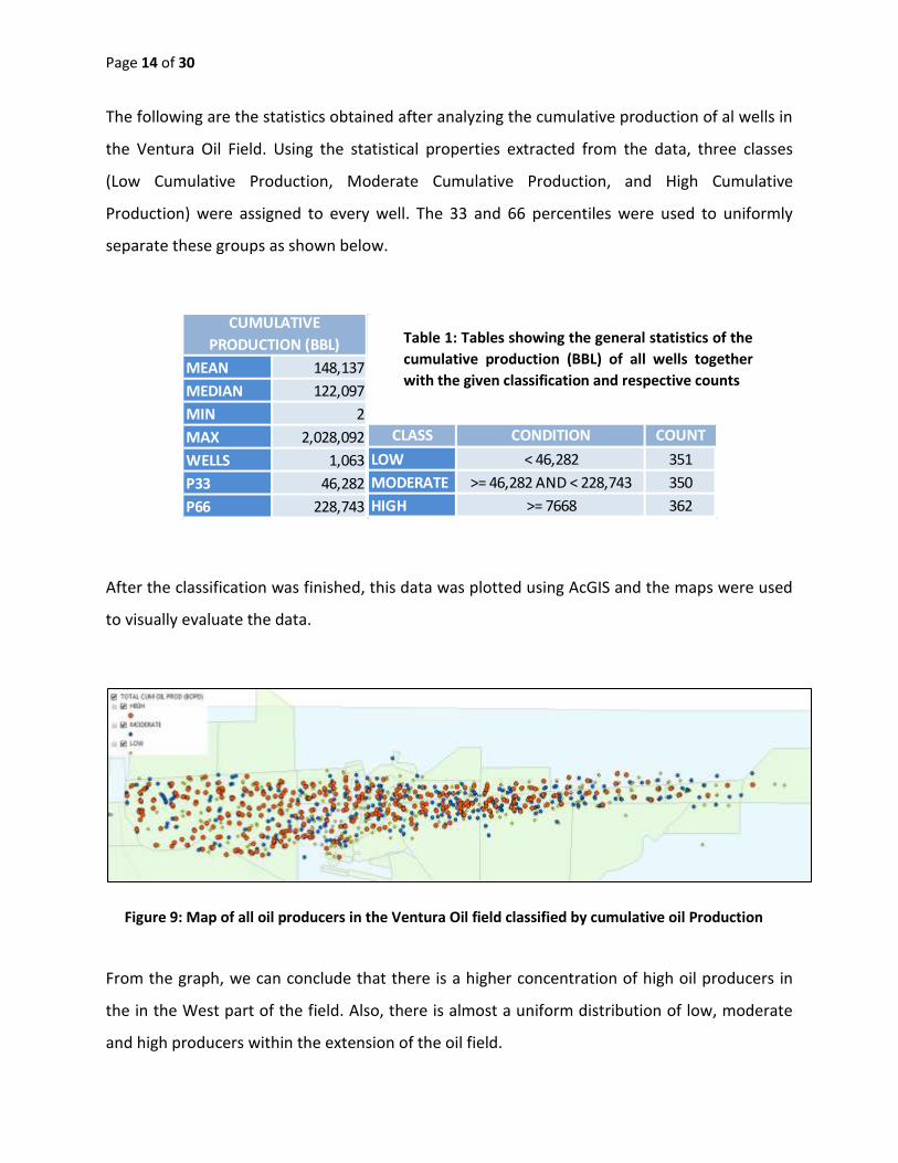
The following are the statistics obtained after analyzing the cumulative production of al wells in

the Ventura Oil Field. Using the statistical properties extracted from the data, three classes

(Low Cumulative Production, Moderate Cumulative Production, and High Cumulative

Production) were assigned to every well. The 33 and 66 percentiles were used to uniformly

separate these groups as shown below.

After the classification was finished, this data was plotted using AcGIS and the maps were used

to visually evaluate the data.

From the graph, we can conclude that there is a higher concentration of high oil producers in

the in the West part of the field. Also, there is almost a uniform distribution of low, moderate

and high producers within the extension of the oil field.

MEAN 148,137

MEDIAN 122,097

MIN 2

MAX 2,028,092

WELLS 1,063

P33 46,282

P66 228,743

CUMULATIVE

PRODUCTION (BBL)

CLASS CONDITION COUNT

LOW < 46,282 351

MODERATE >= 46,282 AND < 228,743 350

HIGH >= 7668 362

Table 1: Tables showing the general statistics of the

cumulative production (BBL) of all wells together

with the given classification and respective counts

Figure 9: Map of all oil producers in the Ventura Oil field classified by cumulative oil Production

Page 15 of 30

For example, directionally drilled wells tend to have better cumulative production than no

directional drilled wells.

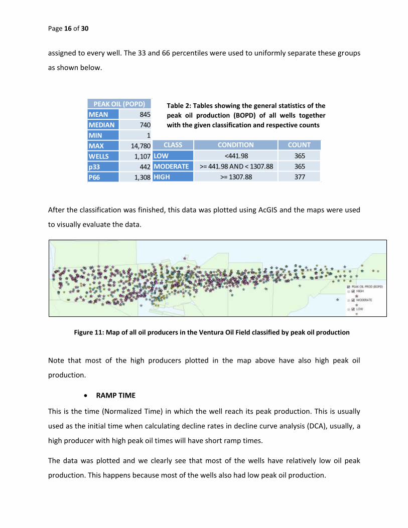
Peak Oil (BOPD)

This is the maximum production of the well within the first 8 months of production. Peak oil

production it usually used as the starting point when performing decline curve analysis (DCA)

The data was plotted and we clearly see that most of the wells have relatively low oil peak

production. This happens because some directionally drilled wells had high initial rates;

therefore most of the wells have relatively low peak oil production.

The following are the statistics obtained after analyzing the peak oil production of all wells in

the Ventura Oil Field. Using the statistical properties extracted from the data, three classes

(Low Peak Oil Production, Moderate Peak Oil Production, and High Peak oil Production) were

Figure 10: Distribution of peak oil production (BOPD) of al wells in the Ventura Oil Field

Page 16 of 30

assigned to every well. The 33 and 66 percentiles were used to uniformly separate these groups

as shown below.

After the classification was finished, this data was plotted using AcGIS and the maps were used

to visually evaluate the data.

Note that most of the high producers plotted in the map above have also high peak oil

production.

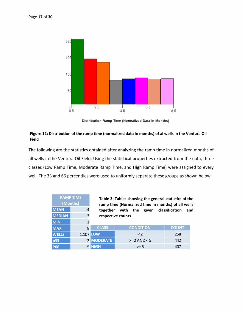
RAMP TIME

This is the time (Normalized Time) in which the well reach its peak production. This is usually

used as the initial time when calculating decline rates in decline curve analysis (DCA), usually, a

high producer with high peak oil times will have short ramp times.

The data was plotted and we clearly see that most of the wells have relatively low oil peak

production. This happens because most of the wells also had low peak oil production.

MEAN 845

MEDIAN 740

MIN 1

MAX 14,780

WELLS 1,107

p33 442

P66 1,308

PEAK OIL (POPD)

CLASS CONDITION COUNT

LOW <441.98 365

MODERATE >= 441.98 AND < 1307.88 365

HIGH >= 1307.88 377

Table 2: Tables showing the general statistics of the

peak oil production (BOPD) of all wells together

with the given classification and respective counts

Figure 11: Map of all oil producers in the Ventura Oil Field classified by peak oil production

Page 17 of 30

The following are the statistics obtained after analyzing the ramp time in normalized months of

all wells in the Ventura Oil Field. Using the statistical properties extracted from the data, three

classes (Low Ramp Time, Moderate Ramp Time, and High Ramp Time) were assigned to every

well. The 33 and 66 percentiles were used to uniformly separate these groups as shown below.

MEAN 4

MEDIAN 3

MIN 1

MAX 8

WELLS 1,107

p33 2

P66 5

RAMP TIME

(Months)

CLASS CONDITION COUNT

LOW < 2 258

MODERATE >= 2 AND < 5 442

HIGH >= 5 407

Table 3: Tables showing the general statistics of the

ramp time (Normalized time in months) of all wells

together with the given classification and

respective counts

Figure 12: Distribution of the ramp time (normalized data in months) of al wells in the Ventura Oil

Field

Page 18 of 30

Finally, using the classification described above, geographical locations, well type, and

normalized time, normalized production graphs were generated.

Data Modeling

Data Preprocessing

Data collected from the data preparation stage was used as inputs to build the unsupervised

descriptive model. Attributes with non-changing instances were removed while attributes with

varied instances were kept to reduce data dimension and irrelevant attributes. Nominal and

Numeric attribute types were defined and separated. Well identification, well status, and

descriptive attributes were defined as nominal. Production, time, depth, pressure, and

hydrocarbon properties were considered as numeric attributes. Figure 14 below shows the 50

input attributes.

0

10

20

30

40

50

60

70

80

90

100

1 6

11

16

21

26

31

36

41

46

51

56

61

66

71

76

81

86

91

96

10

1

10

6

11

1

11

6

Oil

Pro

du

ctio

n (

BO

PD

)

Nomralized Time (Months)

Normalized Oil Produciton

Figure 13: Normalized production for the first 10 years of all oil producers with low Ramp Time, low

Class peak oil, and Low Total production.

Page 19 of 30

Figure 14: Input Attributes

The class attribute was chosen to be the total oil production descriptive class of low, moderate,

and high. Because the numeric attributes vary based on its measured units, normalization was

necessary for data mining comparison between attributes. Normalization with a scale from zero

to one was implemented.

Sampling and Modeling

To test the quality of the data, 80 percent of the entire data set was taken for training and 20

percent was taken for testing. A comparison of the output by the trained model was done on

both the training data set and the testing data set. The sampling was done with Weka

supervised resample filter. To create a descriptive model, Simple K-means was considered, the

model consists of 3 sub-models with 3 clusters, 5 clusters, and 10 clusters. Overfitting was

tested with the 3 sub model in ascending order for consistency of the data. At high number of

clusters, the data set can confuse noisy data for real data or missing data. Therefore, a creation

of 3 sub-models is necessary.

Page 20 of 30

Result

A comparison between the 80 percent cluster output and the 20 percent cluster output

resulted in a perfect match. The training set contains the same percentage of instances

clustered as the testing set. This indicates that the sampled data sets were representative of

one another. Figure 15, 16, and 17 below shows the results from cluster 3, 5, and 10 between

the evaluated training set and testing set.

Figure 15: 3 Cluster Model

Figure 16: 5 Cluster Model

Figure 17:10 Cluster Model

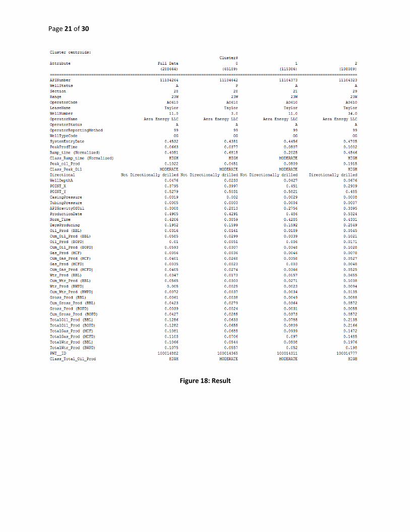
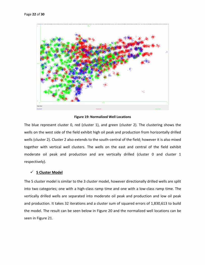
3 Cluster Model

The 3 cluster model shows areas of moderate production and areas of high production from

horizontal and vertical wells. It takes 11 iterations and a cluster sum of squared errors of

1,969,764 to build the model. The result can be seen below in Figure 18 and the normalized

well locations can be seen in Figure 19.

Training Set Testing Set

Training Set Testing Set

Training Set Testing Set

Page 21 of 30

Figure 18: Result

Page 22 of 30

Figure 19: Normalized Well Locations

The blue represent cluster 0, red (cluster 1), and green (cluster 2). The clustering shows the

wells on the west side of the field exhibit high oil peak and production from horizontally drilled

wells (cluster 2). Cluster 2 also extends to the south-central of the field; however it is also mixed

together with vertical well clusters. The wells on the east and central of the field exhibit

moderate oil peak and production and are vertically drilled (cluster 0 and cluster 1

respectively).

5 Cluster Model

The 5 cluster model is similar to the 3 cluster model, however directionally drilled wells are split

into two categories; one with a high-class ramp time and one with a low-class ramp time. The

vertically drilled wells are separated into moderate oil peak and production and low oil peak

and production. It takes 32 iterations and a cluster sum of squared errors of 1,830,613 to build

the model. The result can be seen below in Figure 20 and the normalized well locations can be

seen in Figure 21.

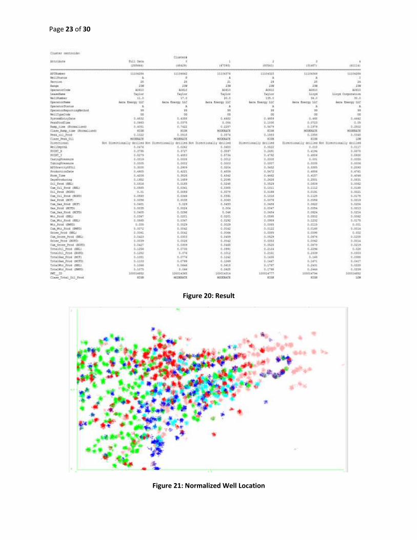
Page 23 of 30

Figure 20: Result

Figure 21: Normalized Well Location

Page 24 of 30

The blue represent cluster 0, red (cluster 1), green (cluster 2), teal (cluster 3), and pink (cluster

4). The two horizontally drilled well clusters exhibit high oil peak and production, wells on the

west side (cluster 2) exhibit high ramp time while south central (cluster 3) wells have moderate

ramp time. The vertically drilled wells on the east side (cluster 4) of the field have low oil peak

and production while the wells at the center (cluster 0 and cluster 1) of the field have moderate

oil peak and production. All of the vertical wells have moderate ramp time.

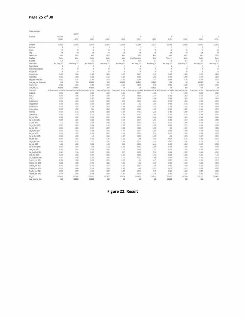
10 Cluster Model

The 10 cluster model clusters the horizontal and vertical wells into clusters with low, moderate,

and high production scattered across the field. Some clusters show signs of over fitting and can

be disregarded from the data set. It takes 29 iterations and a cluster sum of squared errors of

1,681,103 to build the model. The result can be seen below in Figure 22 and the normalized

well locations can be seen in Figure 23.

Page 25 of 30

Figure 22: Result

Page 26 of 30

Figure 23: Normalized Well Location

The blue represent cluster 0, red (cluster 1), green (cluster 2), teal (cluster 3), pink (cluster 4),

purple (cluster 5), orange (cluster 6), dark red (cluster 7), yellow (cluster 8), and black (cluster

9). The result shows 3 different clusters of horizontally drilled wells with high oil peak and

production, the west side of the field have high ramp time (cluster 2) or moderate ramp time

(cluster 8) and wells in south-central (cluster 3) with moderate ramp time. There is a cluster of

horizontal wells scattered around the east and central of the field that shows low peak and

production (cluster 9). They accumulate mainly in the east-south central of the field and

account for 8 percent of the testing instances. This inconsistency in the data set might be an

indication of overfitting due to its small size. This could also be an indication of noise.

Vertical wells in the east side (cluster 4) of the field have low oil peak and production with

moderate ramp time. While the southwest central (cluster 0) and southeast (cluster 6) wells

have moderate oil peak and production with high ramp time. Vertical wells in the north-east

central (cluster 1) have moderate oil peak and production while wells in the direct center

(cluster 5) have high oil production with moderate oil peak. There is a cluster of vertical wells

scattered around the west and central of the field that have high oil peak and production with

Page 27 of 30

low ramp time. They accumulate mainly in the northwest of the field and account for 7 percent

of the test instances. This inconsistency in the data set might also be an indication of overfitting

due to its small size, and could be an indication of noise.

Conclusion:

The field currently has mostly vertical wells that cover around 60% of the total number of wells

drilled. If new horizontal wells were drilled or over existing vertical wells in the west or south-

central of the field, according to the results extracted from the clustering model, the wells will

likely exhibit high oil peak and production with either high or moderate ramp time. If vertical

wells were drilled in the east side of the field, it is most likely going to have low oil peak and

production. However, there is not enough information on horizontal wells in this area;

therefore production of horizontal wells drilled in this area cannot be evaluated. This might be

due to the restraint of obtaining horizontal drilling permits or that the low production may

dissuade horizontal drilling.

If vertical wells were drilled in the center of the field, it is most likely going to have moderate oil

peak and production with moderate ramp time, however, there is also a chance that the field

will output high oil production with moderate peak and ramp time.

Implementation of This Project:

Since the recommendation of our study is encouraging the use of successful horizontal wells,

below is a real life example of horizontal well successfully being used in Ventura County:

Tri-Valley Corp. has drilled seven horizontal wells in its Oxnard fields to get at the heavy oil

there. These wells are drilled down vertically and over horizontally. It then pumps steam into

those wells and pumps oil out. Using SAGD means it will drill another horizontal well above the

existing well. This "injection well" will be used to pump in steam. The steam reduces the

viscosity of the oil so it becomes thinner and moves into the lower well. The heated oil and

water is then pumped to the surface and separated, with the water being cleaned and reused

for a new steam generation. These types of wells can get up to 60 percent of oil from a deposit.

Tri-Valley Corp. is using a steam injection process to wring thick, tar-like oil out of the sands of

Page 28 of 30

its Pleasant Valley field. The Oxnard property yielded 333 barrels of oil a day in May, up from

both March and April, (with March being the previous peak production at 256 barrels).

For successful implementation of this project in real life scenario, it will require an adequate

amount of data for accurate production forecasting so that the training model can be made

more efficient. Also, the field personnel needs to be trained in using software such as WEKA ,

VBA etc. Also, data with less error and noise is preferred. The main advantage of this project

methodology is that it can be cost effective for small fields too. This is because it requires less

development time and the data requirements are flexible as it can be continuously improved as

we accumulate data.

Page 29 of 30

References:

1. California Oil and Gas Fields, Volumes I, II and III. Vol. I (1998), Vol. II (1992), Vol. III

(1982). California Department of Conservation, Division of Oil, Gas, and Geothermal

Resources (DOGGR). 1,472 pp. Ventura Oil Field information pp. 572-574. PDF file

available on CD from www.consrv.ca.gov.

2. California Department of Conservation, Oil and Gas Statistics, Annual Report, December

31, 2006.

3. DOGGR Website