Embed Size (px)
Citation preview
INTRODUCTION
TO
MACHINE LEARNING
AN EARLY DRAFT OF A PROPOSED
TEXTBOOK
Nils J. Nilsson
Robotics Laboratory
Department of Computer Science
Stanford University
Stanford, CA 94305
e-mail: [email protected]
November 3, 1998
Copyright c©2005 Nils J. Nilsson
This material may not be copied, reproduced, or distributed without thewritten permission of the copyright holder.

ii
Contents
1 Preliminaries 1
1.1 Introduction . . . . . . . . . . . . . . . . . . . . . . . . . . . . . . 1
1.1.1 What is Machine Learning? . . . . . . . . . . . . . . . . . 1
1.1.2 Wellsprings of Machine Learning . . . . . . . . . . . . . . 3
1.1.3 Varieties of Machine Learning . . . . . . . . . . . . . . . . 4
1.2 Learning Input-Output Functions . . . . . . . . . . . . . . . . . . 5
1.2.1 Types of Learning . . . . . . . . . . . . . . . . . . . . . . 5
1.2.2 Input Vectors . . . . . . . . . . . . . . . . . . . . . . . . . 7
1.2.3 Outputs . . . . . . . . . . . . . . . . . . . . . . . . . . . . 8
1.2.4 Training Regimes . . . . . . . . . . . . . . . . . . . . . . . 8
1.2.5 Noise . . . . . . . . . . . . . . . . . . . . . . . . . . . . . 9
1.2.6 Performance Evaluation . . . . . . . . . . . . . . . . . . . 9
1.3 Learning Requires Bias . . . . . . . . . . . . . . . . . . . . . . . . 9
1.4 Sample Applications . . . . . . . . . . . . . . . . . . . . . . . . . 11
1.5 Sources . . . . . . . . . . . . . . . . . . . . . . . . . . . . . . . . 13
1.6 Bibliographical and Historical Remarks . . . . . . . . . . . . . . 13
2 Boolean Functions 15
2.1 Representation . . . . . . . . . . . . . . . . . . . . . . . . . . . . 15
2.1.1 Boolean Algebra . . . . . . . . . . . . . . . . . . . . . . . 15
2.1.2 Diagrammatic Representations . . . . . . . . . . . . . . . 16
2.2 Classes of Boolean Functions . . . . . . . . . . . . . . . . . . . . 17
2.2.1 Terms and Clauses . . . . . . . . . . . . . . . . . . . . . . 17
2.2.2 DNF Functions . . . . . . . . . . . . . . . . . . . . . . . . 18
2.2.3 CNF Functions . . . . . . . . . . . . . . . . . . . . . . . . 21
2.2.4 Decision Lists . . . . . . . . . . . . . . . . . . . . . . . . . 22
2.2.5 Symmetric and Voting Functions . . . . . . . . . . . . . . 23
2.2.6 Linearly Separable Functions . . . . . . . . . . . . . . . . 23
2.3 Summary . . . . . . . . . . . . . . . . . . . . . . . . . . . . . . . 24
2.4 Bibliographical and Historical Remarks . . . . . . . . . . . . . . 25
iii
3 Using Version Spaces for Learning 27
3.1 Version Spaces and Mistake Bounds . . . . . . . . . . . . . . . . 27
3.2 Version Graphs . . . . . . . . . . . . . . . . . . . . . . . . . . . . 29
3.3 Learning as Search of a Version Space . . . . . . . . . . . . . . . 32
3.4 The Candidate Elimination Method . . . . . . . . . . . . . . . . 32
3.5 Bibliographical and Historical Remarks . . . . . . . . . . . . . . 34
4 Neural Networks 35
4.1 Threshold Logic Units . . . . . . . . . . . . . . . . . . . . . . . . 35
4.1.1 Definitions and Geometry . . . . . . . . . . . . . . . . . . 35
4.1.2 Special Cases of Linearly Separable Functions . . . . . . . 37
4.1.3 Error-Correction Training of a TLU . . . . . . . . . . . . 38
4.1.4 Weight Space . . . . . . . . . . . . . . . . . . . . . . . . . 40
4.1.5 The Widrow-Hoff Procedure . . . . . . . . . . . . . . . . . 42
4.1.6 Training a TLU on Non-Linearly-Separable Training Sets 44
4.2 Linear Machines . . . . . . . . . . . . . . . . . . . . . . . . . . . 44
4.3 Networks of TLUs . . . . . . . . . . . . . . . . . . . . . . . . . . 46
4.3.1 Motivation and Examples . . . . . . . . . . . . . . . . . . 46
4.3.2 Madalines . . . . . . . . . . . . . . . . . . . . . . . . . . . 49
4.3.3 Piecewise Linear Machines . . . . . . . . . . . . . . . . . . 50
4.3.4 Cascade Networks . . . . . . . . . . . . . . . . . . . . . . 51
4.4 Training Feedforward Networks by Backpropagation . . . . . . . 52
4.4.1 Notation . . . . . . . . . . . . . . . . . . . . . . . . . . . . 52
4.4.2 The Backpropagation Method . . . . . . . . . . . . . . . . 53
4.4.3 Computing Weight Changes in the Final Layer . . . . . . 56
4.4.4 Computing Changes to the Weights in Intermediate Layers 58
4.4.5 Variations on Backprop . . . . . . . . . . . . . . . . . . . 59
4.4.6 An Application: Steering a Van . . . . . . . . . . . . . . . 60
4.5 Synergies Between Neural Network and Knowledge-Based Methods 61
4.6 Bibliographical and Historical Remarks . . . . . . . . . . . . . . 61
5 Statistical Learning 63
5.1 Using Statistical Decision Theory . . . . . . . . . . . . . . . . . . 63
5.1.1 Background and General Method . . . . . . . . . . . . . . 63
5.1.2 Gaussian (or Normal) Distributions . . . . . . . . . . . . 65
5.1.3 Conditionally Independent Binary Components . . . . . . 68
5.2 Learning Belief Networks . . . . . . . . . . . . . . . . . . . . . . 70
5.3 Nearest-Neighbor Methods . . . . . . . . . . . . . . . . . . . . . . 70
5.4 Bibliographical and Historical Remarks . . . . . . . . . . . . . . 72
iv
6 Decision Trees 73
6.1 Definitions . . . . . . . . . . . . . . . . . . . . . . . . . . . . . . . 73
6.2 Supervised Learning of Univariate Decision Trees . . . . . . . . . 74
6.2.1 Selecting the Type of Test . . . . . . . . . . . . . . . . . . 75
6.2.2 Using Uncertainty Reduction to Select Tests . . . . . . . 75
6.2.3 Non-Binary Attributes . . . . . . . . . . . . . . . . . . . . 79
6.3 Networks Equivalent to Decision Trees . . . . . . . . . . . . . . . 79
6.4 Overfitting and Evaluation . . . . . . . . . . . . . . . . . . . . . 80
6.4.1 Overfitting . . . . . . . . . . . . . . . . . . . . . . . . . . 80
6.4.2 Validation Methods . . . . . . . . . . . . . . . . . . . . . 81
6.4.3 Avoiding Overfitting in Decision Trees . . . . . . . . . . . 82
6.4.4 Minimum-Description Length Methods . . . . . . . . . . . 83
6.4.5 Noise in Data . . . . . . . . . . . . . . . . . . . . . . . . . 84
6.5 The Problem of Replicated Subtrees . . . . . . . . . . . . . . . . 84
6.6 The Problem of Missing Attributes . . . . . . . . . . . . . . . . . 86
6.7 Comparisons . . . . . . . . . . . . . . . . . . . . . . . . . . . . . 86
6.8 Bibliographical and Historical Remarks . . . . . . . . . . . . . . 87
7 Inductive Logic Programming 89
7.1 Notation and Definitions . . . . . . . . . . . . . . . . . . . . . . . 90
7.2 A Generic ILP Algorithm . . . . . . . . . . . . . . . . . . . . . . 91
7.3 An Example . . . . . . . . . . . . . . . . . . . . . . . . . . . . . . 94
7.4 Inducing Recursive Programs . . . . . . . . . . . . . . . . . . . . 98
7.5 Choosing Literals to Add . . . . . . . . . . . . . . . . . . . . . . 100
7.6 Relationships Between ILP and Decision Tree Induction . . . . . 101
7.7 Bibliographical and Historical Remarks . . . . . . . . . . . . . . 104
8 Computational Learning Theory 107
8.1 Notation and Assumptions for PAC Learning Theory . . . . . . . 107
8.2 PAC Learning . . . . . . . . . . . . . . . . . . . . . . . . . . . . . 109
8.2.1 The Fundamental Theorem . . . . . . . . . . . . . . . . . 109
8.2.2 Examples . . . . . . . . . . . . . . . . . . . . . . . . . . . 111
8.2.3 Some Properly PAC-Learnable Classes . . . . . . . . . . . 112
8.3 The Vapnik-Chervonenkis Dimension . . . . . . . . . . . . . . . . 113
8.3.1 Linear Dichotomies . . . . . . . . . . . . . . . . . . . . . . 113
8.3.2 Capacity . . . . . . . . . . . . . . . . . . . . . . . . . . . 115
8.3.3 A More General Capacity Result . . . . . . . . . . . . . . 116
8.3.4 Some Facts and Speculations About the VC Dimension . 117
8.4 VC Dimension and PAC Learning . . . . . . . . . . . . . . . . . 118
8.5 Bibliographical and Historical Remarks . . . . . . . . . . . . . . 118
v
9 Unsupervised Learning 119
9.1 What is Unsupervised Learning? . . . . . . . . . . . . . . . . . . 119
9.2 Clustering Methods . . . . . . . . . . . . . . . . . . . . . . . . . . 120
9.2.1 A Method Based on Euclidean Distance . . . . . . . . . . 120
9.2.2 A Method Based on Probabilities . . . . . . . . . . . . . . 124
9.3 Hierarchical Clustering Methods . . . . . . . . . . . . . . . . . . 125
9.3.1 A Method Based on Euclidean Distance . . . . . . . . . . 125
9.3.2 A Method Based on Probabilities . . . . . . . . . . . . . . 126
9.4 Bibliographical and Historical Remarks . . . . . . . . . . . . . . 130
10 Temporal-Difference Learning 131
10.1 Temporal Patterns and Prediction Problems . . . . . . . . . . . . 131
10.2 Supervised and Temporal-Difference Methods . . . . . . . . . . . 131
10.3 Incremental Computation of the (∆W)i . . . . . . . . . . . . . . 134
10.4 An Experiment with TD Methods . . . . . . . . . . . . . . . . . 135
10.5 Theoretical Results . . . . . . . . . . . . . . . . . . . . . . . . . . 138
10.6 Intra-Sequence Weight Updating . . . . . . . . . . . . . . . . . . 138
10.7 An Example Application: TD-gammon . . . . . . . . . . . . . . . 140
10.8 Bibliographical and Historical Remarks . . . . . . . . . . . . . . 141
11 Delayed-Reinforcement Learning 143
11.1 The General Problem . . . . . . . . . . . . . . . . . . . . . . . . 143
11.2 An Example . . . . . . . . . . . . . . . . . . . . . . . . . . . . . . 144
11.3 Temporal Discounting and Optimal Policies . . . . . . . . . . . . 145
11.4 Q-Learning . . . . . . . . . . . . . . . . . . . . . . . . . . . . . . 147
11.5 Discussion, Limitations, and Extensions of Q-Learning . . . . . . 150
11.5.1 An Illustrative Example . . . . . . . . . . . . . . . . . . . 150
11.5.2 Using Random Actions . . . . . . . . . . . . . . . . . . . 152
11.5.3 Generalizing Over Inputs . . . . . . . . . . . . . . . . . . 153
11.5.4 Partially Observable States . . . . . . . . . . . . . . . . . 154
11.5.5 Scaling Problems . . . . . . . . . . . . . . . . . . . . . . . 154
11.6 Bibliographical and Historical Remarks . . . . . . . . . . . . . . 155
vi
12 Explanation-Based Learning 157
12.1 Deductive Learning . . . . . . . . . . . . . . . . . . . . . . . . . . 157
12.2 Domain Theories . . . . . . . . . . . . . . . . . . . . . . . . . . . 158
12.3 An Example . . . . . . . . . . . . . . . . . . . . . . . . . . . . . . 159
12.4 Evaluable Predicates . . . . . . . . . . . . . . . . . . . . . . . . . 162
12.5 More General Proofs . . . . . . . . . . . . . . . . . . . . . . . . . 164
12.6 Utility of EBL . . . . . . . . . . . . . . . . . . . . . . . . . . . . 164
12.7 Applications . . . . . . . . . . . . . . . . . . . . . . . . . . . . . . 164
12.7.1 Macro-Operators in Planning . . . . . . . . . . . . . . . . 164
12.7.2 Learning Search Control Knowledge . . . . . . . . . . . . 167
12.8 Bibliographical and Historical Remarks . . . . . . . . . . . . . . 168
vii

viii

Preface
These notes are in the process of becoming a textbook. The process is quiteunfinished, and the author solicits corrections, criticisms, and suggestions fromstudents and other readers. Although I have tried to eliminate errors, some un-doubtedly remain—caveat lector. Many typographical infelicities will no doubtpersist until the final version. More material has yet to be added. Please let Some of my plans for additions and
other reminders are mentioned inmarginal notes.
me have your suggestions about topics that are too important to be left out.I hope that future versions will cover Hopfield nets, Elman nets and other re-current nets, radial basis functions, grammar and automata learning, geneticalgorithms, and Bayes networks . . .. I am also collecting exercises and projectsuggestions which will appear in future versions.
My intention is to pursue a middle ground between a theoretical textbookand one that focusses on applications. The book concentrates on the importantideas in machine learning. I do not give proofs of many of the theorems that Istate, but I do give plausibility arguments and citations to formal proofs. And, Ido not treat many matters that would be of practical importance in applications;the book is not a handbook of machine learning practice. Instead, my goal isto give the reader sufficient preparation to make the extensive literature onmachine learning accessible.
Students in my Stanford courses on machine learning have already madeseveral useful suggestions, as have my colleague, Pat Langley, and my teachingassistants, Ron Kohavi, Karl Pfleger, Robert Allen, and Lise Getoor.
ix
Chapter 1
Preliminaries
1.1 Introduction
1.1.1 What is Machine Learning?
Learning, like intelligence, covers such a broad range of processes that it is dif-ficult to define precisely. A dictionary definition includes phrases such as “togain knowledge, or understanding of, or skill in, by study, instruction, or expe-rience,” and “modification of a behavioral tendency by experience.” Zoologistsand psychologists study learning in animals and humans. In this book we fo-cus on learning in machines. There are several parallels between animal andmachine learning. Certainly, many techniques in machine learning derive fromthe efforts of psychologists to make more precise their theories of animal andhuman learning through computational models. It seems likely also that theconcepts and techniques being explored by researchers in machine learning mayilluminate certain aspects of biological learning.
As regards machines, we might say, very broadly, that a machine learnswhenever it changes its structure, program, or data (based on its inputs or inresponse to external information) in such a manner that its expected futureperformance improves. Some of these changes, such as the addition of a recordto a data base, fall comfortably within the province of other disciplines and arenot necessarily better understood for being called learning. But, for example,when the performance of a speech-recognition machine improves after hearingseveral samples of a person’s speech, we feel quite justified in that case to saythat the machine has learned.
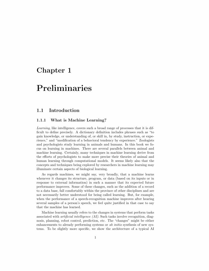
Machine learning usually refers to the changes in systems that perform tasksassociated with artificial intelligence (AI). Such tasks involve recognition, diag-nosis, planning, robot control, prediction, etc. The “changes” might be eitherenhancements to already performing systems or ab initio synthesis of new sys-tems. To be slightly more specific, we show the architecture of a typical AI
1
2 CHAPTER 1. PRELIMINARIES
“agent” in Fig. 1.1. This agent perceives and models its environment and com-putes appropriate actions, perhaps by anticipating their effects. Changes madeto any of the components shown in the figure might count as learning. Differentlearning mechanisms might be employed depending on which subsystem is beingchanged. We will study several different learning methods in this book.
Sensory signals
Perception
Actions
ActionComputation
ModelPlanning andReasoning
Goals
Figure 1.1: An AI System
One might ask “Why should machines have to learn? Why not design ma-chines to perform as desired in the first place?” There are several reasons whymachine learning is important. Of course, we have already mentioned that theachievement of learning in machines might help us understand how animals andhumans learn. But there are important engineering reasons as well. Some ofthese are:
• Some tasks cannot be defined well except by example; that is, we might beable to specify input/output pairs but not a concise relationship betweeninputs and desired outputs. We would like machines to be able to adjusttheir internal structure to produce correct outputs for a large number ofsample inputs and thus suitably constrain their input/output function toapproximate the relationship implicit in the examples.
• It is possible that hidden among large piles of data are important rela-tionships and correlations. Machine learning methods can often be usedto extract these relationships (data mining).
1.1. INTRODUCTION 3
• Human designers often produce machines that do not work as well asdesired in the environments in which they are used. In fact, certain char-acteristics of the working environment might not be completely knownat design time. Machine learning methods can be used for on-the-jobimprovement of existing machine designs.
• The amount of knowledge available about certain tasks might be too largefor explicit encoding by humans. Machines that learn this knowledgegradually might be able to capture more of it than humans would want towrite down.
• Environments change over time. Machines that can adapt to a changingenvironment would reduce the need for constant redesign.
• New knowledge about tasks is constantly being discovered by humans.Vocabulary changes. There is a constant stream of new events in theworld. Continuing redesign of AI systems to conform to new knowledge isimpractical, but machine learning methods might be able to track muchof it.
1.1.2 Wellsprings of Machine Learning
Work in machine learning is now converging from several sources. These dif-ferent traditions each bring different methods and different vocabulary whichare now being assimilated into a more unified discipline. Here is a brief listingof some of the separate disciplines that have contributed to machine learning;more details will follow in the the appropriate chapters:
• Statistics: A long-standing problem in statistics is how best to use sam-ples drawn from unknown probability distributions to help decide fromwhich distribution some new sample is drawn. A related problem is howto estimate the value of an unknown function at a new point given thevalues of this function at a set of sample points. Statistical methodsfor dealing with these problems can be considered instances of machinelearning because the decision and estimation rules depend on a corpus ofsamples drawn from the problem environment. We will explore some ofthe statistical methods later in the book. Details about the statistical the-ory underlying these methods can be found in statistical textbooks suchas [Anderson, 1958].
• Brain Models: Non-linear elements with weighted inputshave been suggested as simple models of biological neu-rons. Networks of these elements have been studied by sev-eral researchers including [McCulloch & Pitts, 1943, Hebb, 1949,Rosenblatt, 1958] and, more recently by [Gluck & Rumelhart, 1989,Sejnowski, Koch, & Churchland, 1988]. Brain modelers are interestedin how closely these networks approximate the learning phenomena of
4 CHAPTER 1. PRELIMINARIES
living brains. We shall see that several important machine learningtechniques are based on networks of nonlinear elements—often calledneural networks. Work inspired by this school is sometimes calledconnectionism, brain-style computation, or sub-symbolic processing.
• Adaptive Control Theory: Control theorists study the problem of con-trolling a process having unknown parameters which must be estimatedduring operation. Often, the parameters change during operation, and thecontrol process must track these changes. Some aspects of controlling arobot based on sensory inputs represent instances of this sort of problem.For an introduction see [Bollinger & Duffie, 1988].
• Psychological Models: Psychologists have studied the performance ofhumans in various learning tasks. An early example is the EPAM net-work for storing and retrieving one member of a pair of words whengiven another [Feigenbaum, 1961]. Related work led to a number ofearly decision tree [Hunt, Marin, & Stone, 1966] and semantic network[Anderson & Bower, 1973] methods. More recent work of this sort hasbeen influenced by activities in artificial intelligence which we will be pre-senting.
Some of the work in reinforcement learning can be traced to efforts tomodel how reward stimuli influence the learning of goal-seeking behavior inanimals [Sutton & Barto, 1987]. Reinforcement learning is an importanttheme in machine learning research.
• Artificial Intelligence: From the beginning, AI research has been con-cerned with machine learning. Samuel developed a prominent early pro-gram that learned parameters of a function for evaluating board posi-tions in the game of checkers [Samuel, 1959]. AI researchers have alsoexplored the role of analogies in learning [Carbonell, 1983] and how fu-ture actions and decisions can be based on previous exemplary cases[Kolodner, 1993]. Recent work has been directed at discovering rulesfor expert systems using decision-tree methods [Quinlan, 1990] and in-ductive logic programming [Muggleton, 1991, Lavrac & Dzeroski, 1994].Another theme has been saving and generalizing the results of prob-lem solving using explanation-based learning [DeJong & Mooney, 1986,Laird, et al., 1986, Minton, 1988, Etzioni, 1993].
• Evolutionary Models:
In nature, not only do individual animals learn to perform better, butspecies evolve to be better fit in their individual niches. Since the distinc-tion between evolving and learning can be blurred in computer systems,techniques that model certain aspects of biological evolution have beenproposed as learning methods to improve the performance of computerprograms. Genetic algorithms [Holland, 1975] and genetic programming[Koza, 1992, Koza, 1994] are the most prominent computational tech-niques for evolution.
1.2. LEARNING INPUT-OUTPUT FUNCTIONS 5
1.1.3 Varieties of Machine Learning
Orthogonal to the question of the historical source of any learning technique isthe more important question of what is to be learned. In this book, we take itthat the thing to be learned is a computational structure of some sort. We willconsider a variety of different computational structures:
• Functions
• Logic programs and rule sets
• Finite-state machines
• Grammars
• Problem solving systems
We will present methods both for the synthesis of these structures from examplesand for changing existing structures. In the latter case, the change to theexisting structure might be simply to make it more computationally efficientrather than to increase the coverage of the situations it can handle. Much ofthe terminology that we shall be using throughout the book is best introducedby discussing the problem of learning functions, and we turn to that matterfirst.
1.2 Learning Input-Output Functions
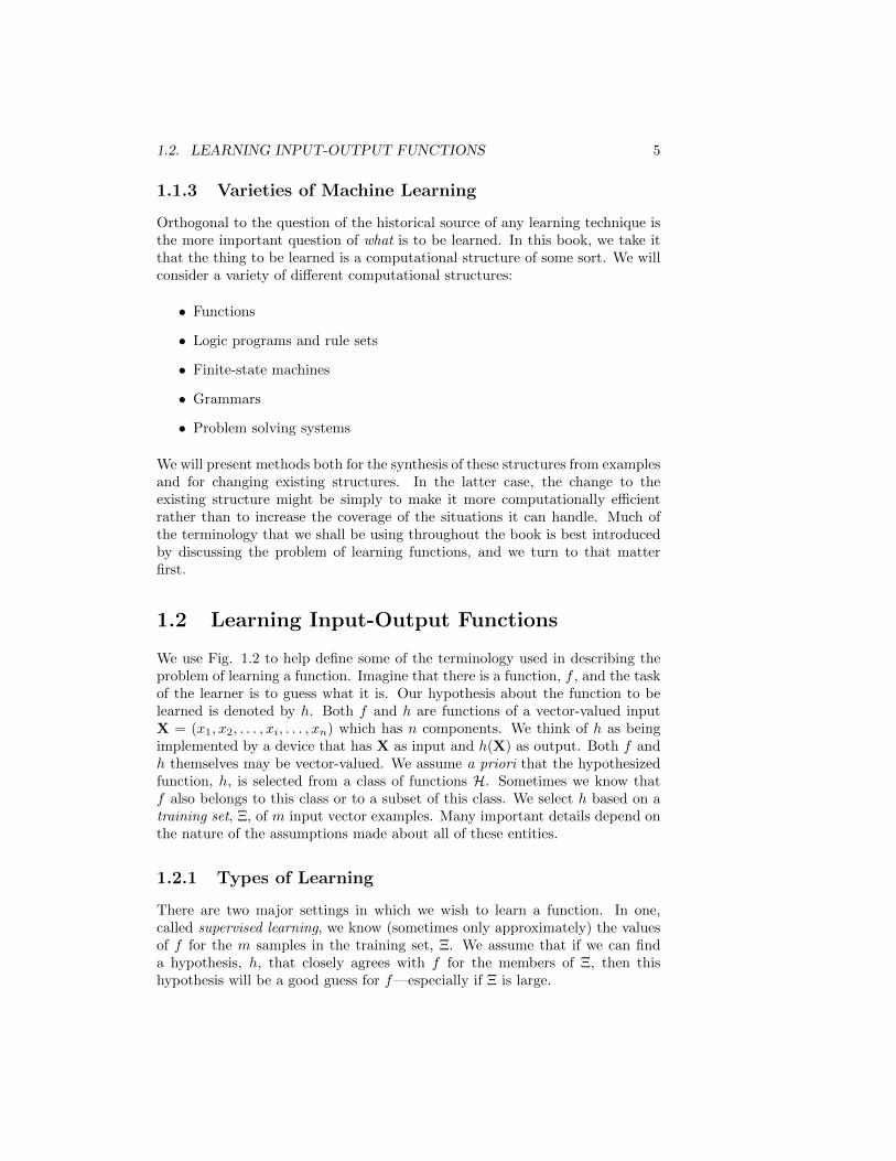
We use Fig. 1.2 to help define some of the terminology used in describing theproblem of learning a function. Imagine that there is a function, f , and the taskof the learner is to guess what it is. Our hypothesis about the function to belearned is denoted by h. Both f and h are functions of a vector-valued inputX = (x1, x2, . . . , xi, . . . , xn) which has n components. We think of h as beingimplemented by a device that has X as input and h(X) as output. Both f andh themselves may be vector-valued. We assume a priori that the hypothesizedfunction, h, is selected from a class of functions H. Sometimes we know thatf also belongs to this class or to a subset of this class. We select h based on atraining set, Ξ, of m input vector examples. Many important details depend onthe nature of the assumptions made about all of these entities.
1.2.1 Types of Learning
There are two major settings in which we wish to learn a function. In one,called supervised learning, we know (sometimes only approximately) the valuesof f for the m samples in the training set, Ξ. We assume that if we can finda hypothesis, h, that closely agrees with f for the members of Ξ, then thishypothesis will be a good guess for f—especially if Ξ is large.
6 CHAPTER 1. PRELIMINARIES
h(X)h
= X1, X2, . . . Xi, . . ., Xm
Training Set:
X =
x1...xi...xn
h H
Figure 1.2: An Input-Output Function
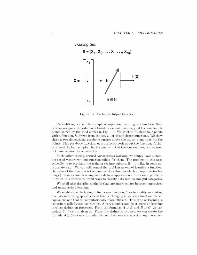
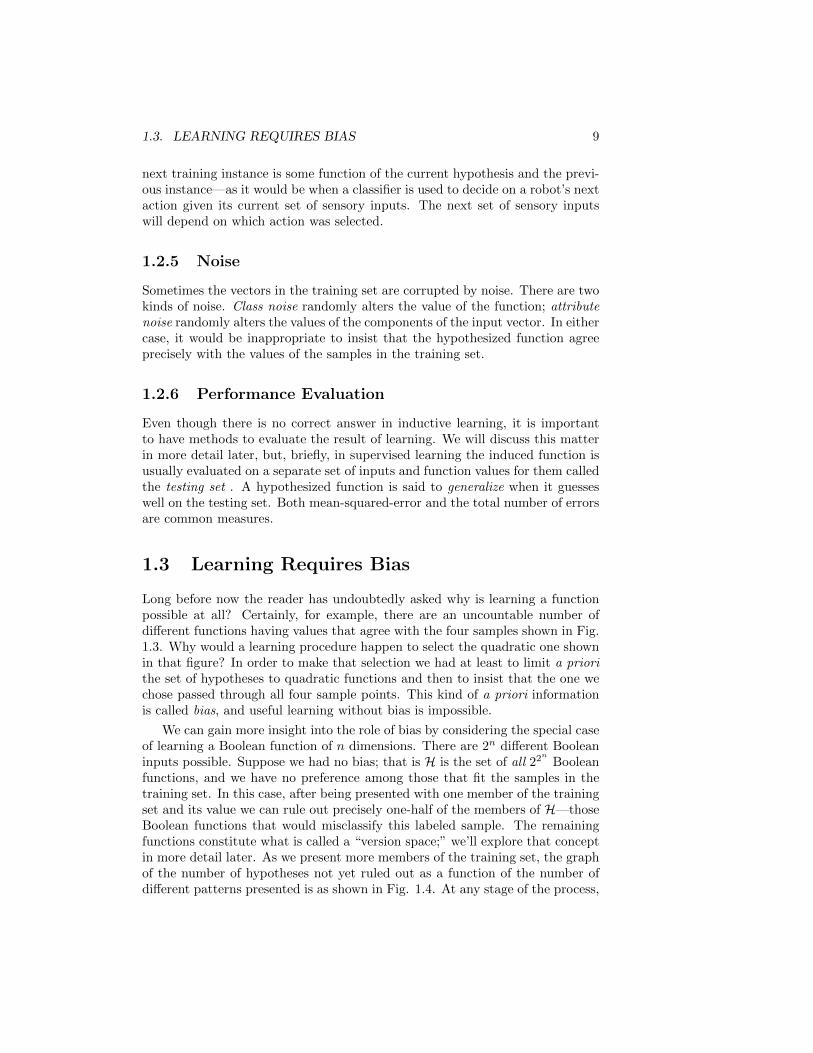
Curve-fitting is a simple example of supervised learning of a function. Sup-pose we are given the values of a two-dimensional function, f , at the four samplepoints shown by the solid circles in Fig. 1.3. We want to fit these four pointswith a function, h, drawn from the set, H, of second-degree functions. We showthere a two-dimensional parabolic surface above the x1, x2 plane that fits thepoints. This parabolic function, h, is our hypothesis about the function, f , thatproduced the four samples. In this case, h = f at the four samples, but we neednot have required exact matches.
In the other setting, termed unsupervised learning, we simply have a train-ing set of vectors without function values for them. The problem in this case,typically, is to partition the training set into subsets, Ξ1, . . . , ΞR, in some ap-propriate way. (We can still regard the problem as one of learning a function;the value of the function is the name of the subset to which an input vector be-longs.) Unsupervised learning methods have application in taxonomic problemsin which it is desired to invent ways to classify data into meaningful categories.
We shall also describe methods that are intermediate between supervisedand unsupervised learning.
We might either be trying to find a new function, h, or to modify an existingone. An interesting special case is that of changing an existing function into anequivalent one that is computationally more efficient. This type of learning issometimes called speed-up learning. A very simple example of speed-up learninginvolves deduction processes. From the formulas A ⊃ B and B ⊃ C, we candeduce C if we are given A. From this deductive process, we can create theformula A ⊃ C—a new formula but one that does not sanction any more con-
1.2. LEARNING INPUT-OUTPUT FUNCTIONS 7
-10-5
05
10-10
-5
0
5
10
0500
1000
1500
-10-5
05
10-10
-5
0
5
10
00000
0
x1
x2
h sample f-value
Figure 1.3: A Surface that Fits Four Points
clusions than those that could be derived from the formulas that we previouslyhad. But with this new formula we can derive C more quickly, given A, thanwe could have done before. We can contrast speed-up learning with methodsthat create genuinely new functions—ones that might give different results afterlearning than they did before. We say that the latter methods involve inductivelearning. As opposed to deduction, there are no correct inductions—only usefulones.
1.2.2 Input Vectors
Because machine learning methods derive from so many different traditions, itsterminology is rife with synonyms, and we will be using most of them in thisbook. For example, the input vector is called by a variety of names. Someof these are: input vector, pattern vector, feature vector, sample, example, andinstance. The components, xi, of the input vector are variously called features,attributes, input variables, and components.
The values of the components can be of three main types. They mightbe real-valued numbers, discrete-valued numbers, or categorical values. As anexample illustrating categorical values, information about a student might berepresented by the values of the attributes class, major, sex, adviser. A par-ticular student would then be represented by a vector such as: (sophomore,history, male, higgins). Additionally, categorical values may be ordered (as insmall, medium, large) or unordered (as in the example just given). Of course,mixtures of all these types of values are possible.
In all cases, it is possible to represent the input in unordered form by listingthe names of the attributes together with their values. The vector form assumesthat the attributes are ordered and given implicitly by a form. As an exampleof an attribute-value representation, we might have: (major: history, sex: male,
8 CHAPTER 1. PRELIMINARIES
class: sophomore, adviser: higgins, age: 19). We will be using the vector formexclusively.
An important specialization uses Boolean values, which can be regarded asa special case of either discrete numbers (1,0) or of categorical variables (True,False).
1.2.3 Outputs
The output may be a real number, in which case the process embodying thefunction, h, is called a function estimator, and the output is called an outputvalue or estimate.
Alternatively, the output may be a categorical value, in which case the pro-cess embodying h is variously called a classifier, a recognizer, or a categorizer,and the output itself is called a label, a class, a category, or a decision. Classi-fiers have application in a number of recognition problems, for example in therecognition of hand-printed characters. The input in that case is some suitablerepresentation of the printed character, and the classifier maps this input intoone of, say, 64 categories.
Vector-valued outputs are also possible with components being real numbersor categorical values.
An important special case is that of Boolean output values. In that case,a training pattern having value 1 is called a positive instance, and a trainingsample having value 0 is called a negative instance. When the input is alsoBoolean, the classifier implements a Boolean function. We study the Booleancase in some detail because it allows us to make important general points ina simplified setting. Learning a Boolean function is sometimes called conceptlearning, and the function is called a concept.
1.2.4 Training Regimes
There are several ways in which the training set, Ξ, can be used to produce ahypothesized function. In the batch method, the entire training set is availableand used all at once to compute the function, h. A variation of this methoduses the entire training set to modify a current hypothesis iteratively until anacceptable hypothesis is obtained. By contrast, in the incremental method, weselect one member at a time from the training set and use this instance aloneto modify a current hypothesis. Then another member of the training set isselected, and so on. The selection method can be random (with replacement)or it can cycle through the training set iteratively. If the entire training setbecomes available one member at a time, then we might also use an incrementalmethod—selecting and using training set members as they arrive. (Alterna-tively, at any stage all training set members so far available could be used in a“batch” process.) Using the training set members as they become available iscalled an online method. Online methods might be used, for example, when the
1.3. LEARNING REQUIRES BIAS 9
next training instance is some function of the current hypothesis and the previ-ous instance—as it would be when a classifier is used to decide on a robot’s nextaction given its current set of sensory inputs. The next set of sensory inputswill depend on which action was selected.
1.2.5 Noise
Sometimes the vectors in the training set are corrupted by noise. There are twokinds of noise. Class noise randomly alters the value of the function; attributenoise randomly alters the values of the components of the input vector. In eithercase, it would be inappropriate to insist that the hypothesized function agreeprecisely with the values of the samples in the training set.
1.2.6 Performance Evaluation
Even though there is no correct answer in inductive learning, it is importantto have methods to evaluate the result of learning. We will discuss this matterin more detail later, but, briefly, in supervised learning the induced function isusually evaluated on a separate set of inputs and function values for them calledthe testing set . A hypothesized function is said to generalize when it guesseswell on the testing set. Both mean-squared-error and the total number of errorsare common measures.
1.3 Learning Requires Bias
Long before now the reader has undoubtedly asked why is learning a functionpossible at all? Certainly, for example, there are an uncountable number ofdifferent functions having values that agree with the four samples shown in Fig.1.3. Why would a learning procedure happen to select the quadratic one shownin that figure? In order to make that selection we had at least to limit a priorithe set of hypotheses to quadratic functions and then to insist that the one wechose passed through all four sample points. This kind of a priori informationis called bias, and useful learning without bias is impossible.
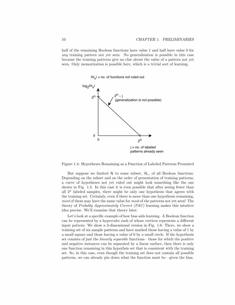
We can gain more insight into the role of bias by considering the special caseof learning a Boolean function of n dimensions. There are 2n different Booleaninputs possible. Suppose we had no bias; that is H is the set of all 22n Booleanfunctions, and we have no preference among those that fit the samples in thetraining set. In this case, after being presented with one member of the trainingset and its value we can rule out precisely one-half of the members of H—thoseBoolean functions that would misclassify this labeled sample. The remainingfunctions constitute what is called a “version space;” we’ll explore that conceptin more detail later. As we present more members of the training set, the graphof the number of hypotheses not yet ruled out as a function of the number ofdifferent patterns presented is as shown in Fig. 1.4. At any stage of the process,
10 CHAPTER 1. PRELIMINARIES
half of the remaining Boolean functions have value 1 and half have value 0 forany training pattern not yet seen. No generalization is possible in this casebecause the training patterns give no clue about the value of a pattern not yetseen. Only memorization is possible here, which is a trivial sort of learning.
log2|Hv|
2n
2n
j = no. of labeledpatterns already seen
00
2n j(generalization is not possible)
|Hv| = no. of functions not ruled out
Figure 1.4: Hypotheses Remaining as a Function of Labeled Patterns Presented
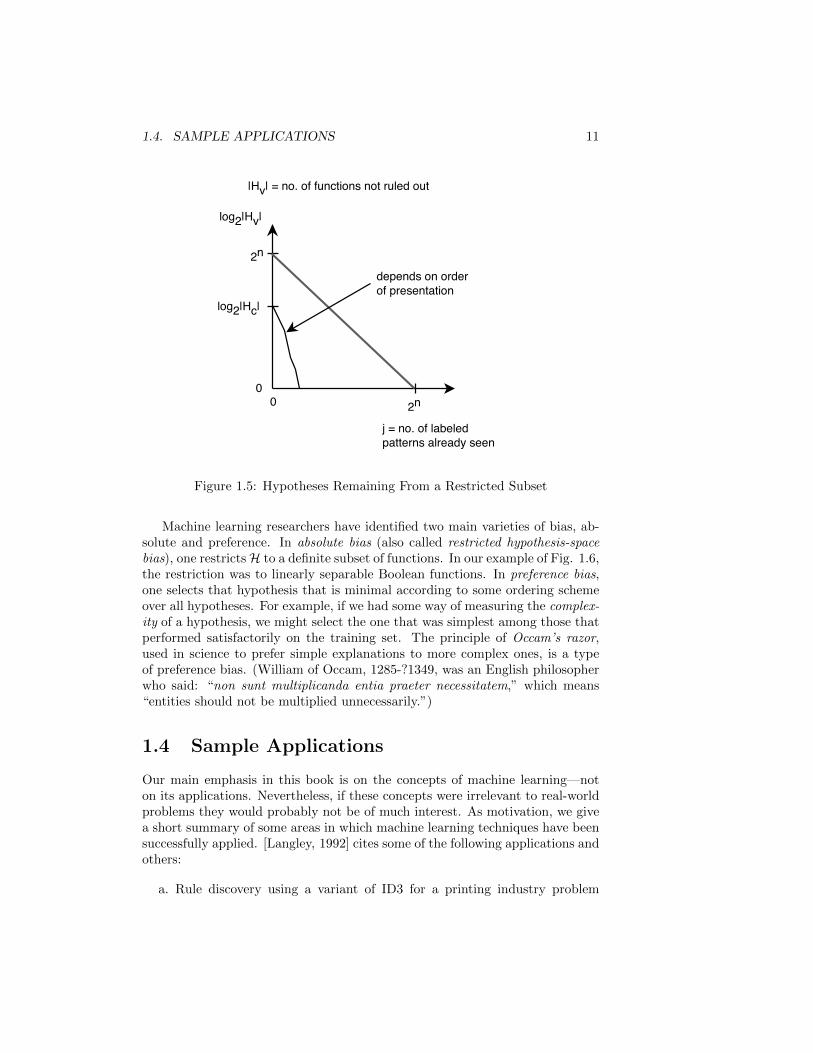
But suppose we limited H to some subset, Hc, of all Boolean functions.Depending on the subset and on the order of presentation of training patterns,a curve of hypotheses not yet ruled out might look something like the oneshown in Fig. 1.5. In this case it is even possible that after seeing fewer thanall 2n labeled samples, there might be only one hypothesis that agrees withthe training set. Certainly, even if there is more than one hypothesis remaining,most of them may have the same value for most of the patterns not yet seen! Thetheory of Probably Approximately Correct (PAC) learning makes this intuitiveidea precise. We’ll examine that theory later.
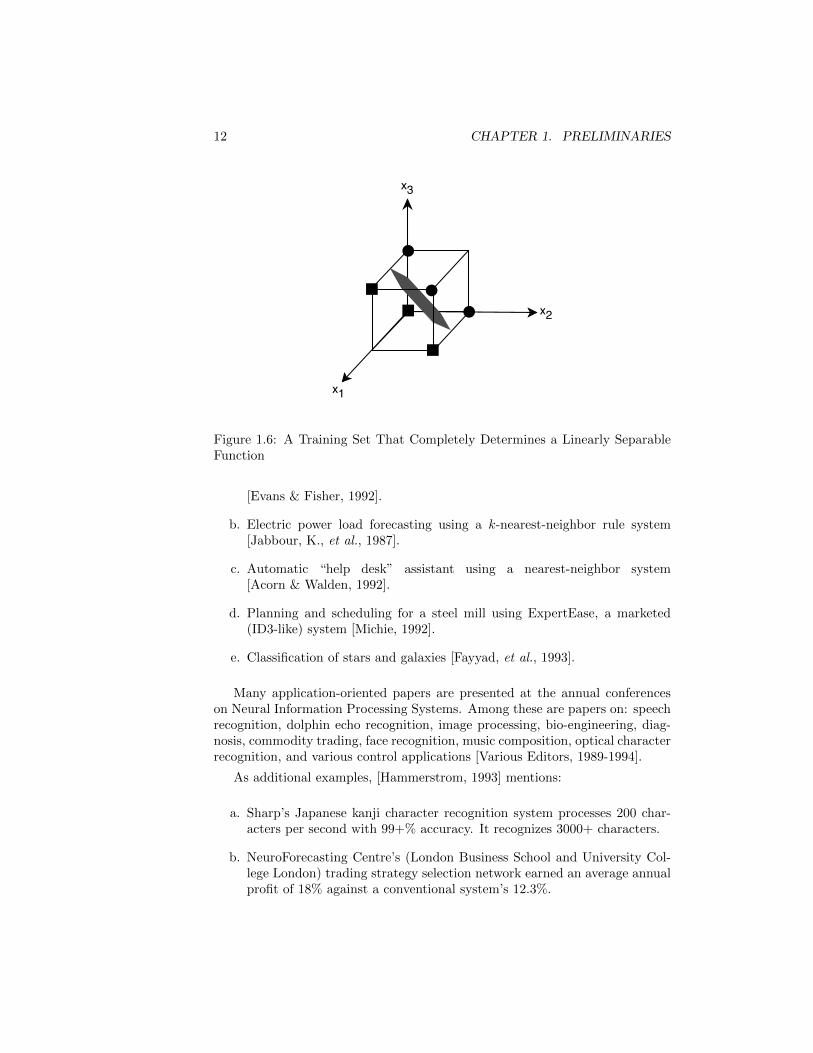
Let’s look at a specific example of how bias aids learning. A Boolean functioncan be represented by a hypercube each of whose vertices represents a differentinput pattern. We show a 3-dimensional version in Fig. 1.6. There, we show atraining set of six sample patterns and have marked those having a value of 1 bya small square and those having a value of 0 by a small circle. If the hypothesisset consists of just the linearly separable functions—those for which the positiveand negative instances can be separated by a linear surface, then there is onlyone function remaining in this hypothsis set that is consistent with the trainingset. So, in this case, even though the training set does not contain all possiblepatterns, we can already pin down what the function must be—given the bias.
1.4. SAMPLE APPLICATIONS 11
log2|Hv|
2n
2n
j = no. of labeledpatterns already seen
00
|Hv| = no. of functions not ruled out
depends on orderof presentation
log2|Hc|
Figure 1.5: Hypotheses Remaining From a Restricted Subset
Machine learning researchers have identified two main varieties of bias, ab-solute and preference. In absolute bias (also called restricted hypothesis-spacebias), one restrictsH to a definite subset of functions. In our example of Fig. 1.6,the restriction was to linearly separable Boolean functions. In preference bias,one selects that hypothesis that is minimal according to some ordering schemeover all hypotheses. For example, if we had some way of measuring the complex-ity of a hypothesis, we might select the one that was simplest among those thatperformed satisfactorily on the training set. The principle of Occam’s razor,used in science to prefer simple explanations to more complex ones, is a typeof preference bias. (William of Occam, 1285-?1349, was an English philosopherwho said: “non sunt multiplicanda entia praeter necessitatem,” which means“entities should not be multiplied unnecessarily.”)
1.4 Sample Applications
Our main emphasis in this book is on the concepts of machine learning—noton its applications. Nevertheless, if these concepts were irrelevant to real-worldproblems they would probably not be of much interest. As motivation, we givea short summary of some areas in which machine learning techniques have beensuccessfully applied. [Langley, 1992] cites some of the following applications andothers:
a. Rule discovery using a variant of ID3 for a printing industry problem
12 CHAPTER 1. PRELIMINARIES
x1
x2
x3
Figure 1.6: A Training Set That Completely Determines a Linearly SeparableFunction
[Evans & Fisher, 1992].
b. Electric power load forecasting using a k-nearest-neighbor rule system[Jabbour, K., et al., 1987].
c. Automatic “help desk” assistant using a nearest-neighbor system[Acorn & Walden, 1992].
d. Planning and scheduling for a steel mill using ExpertEase, a marketed(ID3-like) system [Michie, 1992].
e. Classification of stars and galaxies [Fayyad, et al., 1993].
Many application-oriented papers are presented at the annual conferenceson Neural Information Processing Systems. Among these are papers on: speechrecognition, dolphin echo recognition, image processing, bio-engineering, diag-nosis, commodity trading, face recognition, music composition, optical characterrecognition, and various control applications [Various Editors, 1989-1994].
As additional examples, [Hammerstrom, 1993] mentions:
a. Sharp’s Japanese kanji character recognition system processes 200 char-acters per second with 99+% accuracy. It recognizes 3000+ characters.
b. NeuroForecasting Centre’s (London Business School and University Col-lege London) trading strategy selection network earned an average annualprofit of 18% against a conventional system’s 12.3%.
1.5. SOURCES 13
c. Fujitsu’s (plus a partner’s) neural network for monitoring a continuoussteel casting operation has been in successful operation since early 1990.
In summary, it is rather easy nowadays to find applications of machine learn-ing techniques. This fact should come as no surprise inasmuch as many machinelearning techniques can be viewed as extensions of well known statistical meth-ods which have been successfully applied for many years.
1.5 Sources
Besides the rich literature in machine learning (a small part ofwhich is referenced in the Bibliography), there are several text-books that are worth mentioning [Hertz, Krogh, & Palmer, 1991,Weiss & Kulikowski, 1991, Natarjan, 1991, Fu, 1994, Langley, 1996].[Shavlik & Dietterich, 1990, Buchanan & Wilkins, 1993] are edited vol-umes containing some of the most important papers. A survey paper by[Dietterich, 1990] gives a good overview of many important topics. There arealso well established conferences and publications where papers are given andappear including:
• The Annual Conferences on Advances in Neural Information ProcessingSystems
• The Annual Workshops on Computational Learning Theory
• The Annual International Workshops on Machine Learning
• The Annual International Conferences on Genetic Algorithms
(The Proceedings of the above-listed four conferences are published byMorgan Kaufmann.)
• The journal Machine Learning (published by Kluwer Academic Publish-ers).
There is also much information, as well as programs and datasets, available overthe Internet through the World Wide Web.
1.6 Bibliographical and Historical RemarksTo be added. Every chapter willcontain a brief survey of the historyof the material covered in thatchapter.

14 CHAPTER 1. PRELIMINARIES
Chapter 2
Boolean Functions
2.1 Representation
2.1.1 Boolean Algebra
Many important ideas about learning of functions are most easily presentedusing the special case of Boolean functions. There are several important sub-classes of Boolean functions that are used as hypothesis classes for functionlearning. Therefore, we digress in this chapter to present a review of Booleanfunctions and their properties. (For a more thorough treatment see, for example,[Unger, 1989].)
A Boolean function, f(x1, x2, . . . , xn) maps an n-tuple of (0,1) values to0, 1. Boolean algebra is a convenient notation for representing Boolean func-tions. Boolean algebra uses the connectives ·, +, and . For example, the andfunction of two variables is written x1 · x2. By convention, the connective, “·”is usually suppressed, and the and function is written x1x2. x1x2 has value 1 ifand only if both x1 and x2 have value 1; if either x1 or x2 has value 0, x1x2 hasvalue 0. The (inclusive) or function of two variables is written x1 + x2. x1 + x2
has value 1 if and only if either or both of x1 or x2 has value 1; if both x1 andx2 have value 0, x1 +x2 has value 0. The complement or negation of a variable,x, is written x. x has value 1 if and only if x has value 0; if x has value 1, x hasvalue 0.
These definitions are compactly given by the following rules for Booleanalgebra:
1 + 1 = 1, 1 + 0 = 1, 0 + 0 = 0,
1 · 1 = 1, 1 · 0 = 0, 0 · 0 = 0, and
1 = 0, 0 = 1.
Sometimes the arguments and values of Boolean functions are expressed interms of the constants T (True) and F (False) instead of 1 and 0, respectively.
15
16 CHAPTER 2. BOOLEAN FUNCTIONS
The connectives · and + are each commutative and associative. Thus, forexample, x1(x2x3) = (x1x2)x3, and both can be written simply as x1x2x3.Similarly for +.
A Boolean formula consisting of a single variable, such as x1 is called anatom. One consisting of either a single variable or its complement, such as x1,is called a literal.
The operators · and + do not commute between themselves. Instead, wehave DeMorgan’s laws (which can be verified by using the above definitions):
x1x2 = x1 + x2, and
x1 + x2 = x1 x2.
2.1.2 Diagrammatic Representations
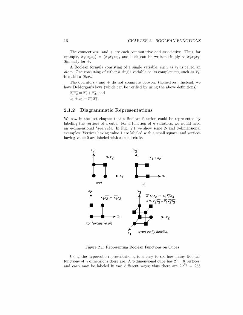
We saw in the last chapter that a Boolean function could be represented bylabeling the vertices of a cube. For a function of n variables, we would needan n-dimensional hypercube. In Fig. 2.1 we show some 2- and 3-dimensionalexamples. Vertices having value 1 are labeled with a small square, and verticeshaving value 0 are labeled with a small circle.
x1
x2
x1
x2
x1
x2
and or
xor (exclusive or)
x1x2 x1 + x2
x1x2 + x1x2
even parity functionx1
x2
x3x1x2x3 + x1x2x3+ x1x2x3 + x1x2x3
Figure 2.1: Representing Boolean Functions on Cubes
Using the hypercube representations, it is easy to see how many Booleanfunctions of n dimensions there are. A 3-dimensional cube has 23 = 8 vertices,and each may be labeled in two different ways; thus there are 2(23) = 256
2.2. CLASSES OF BOOLEAN FUNCTIONS 17
different Boolean functions of 3 variables. In general, there are 22n Booleanfunctions of n variables.
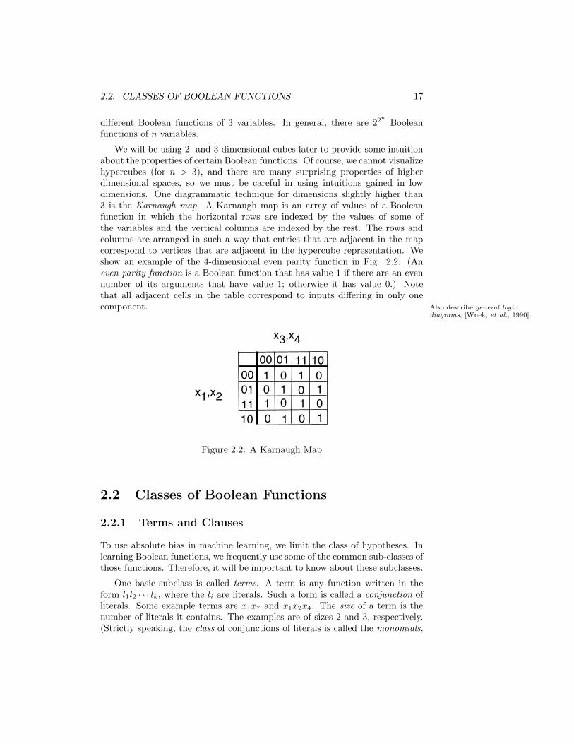
We will be using 2- and 3-dimensional cubes later to provide some intuitionabout the properties of certain Boolean functions. Of course, we cannot visualizehypercubes (for n > 3), and there are many surprising properties of higherdimensional spaces, so we must be careful in using intuitions gained in lowdimensions. One diagrammatic technique for dimensions slightly higher than3 is the Karnaugh map. A Karnaugh map is an array of values of a Booleanfunction in which the horizontal rows are indexed by the values of some ofthe variables and the vertical columns are indexed by the rest. The rows andcolumns are arranged in such a way that entries that are adjacent in the mapcorrespond to vertices that are adjacent in the hypercube representation. Weshow an example of the 4-dimensional even parity function in Fig. 2.2. (Aneven parity function is a Boolean function that has value 1 if there are an evennumber of its arguments that have value 1; otherwise it has value 0.) Notethat all adjacent cells in the table correspond to inputs differing in only onecomponent. Also describe general logic
diagrams, [Wnek, et al., 1990].
00 01 10110001
1011
1 1
11
111
100 0
00
00
0
x1,x2
x3,x4
Figure 2.2: A Karnaugh Map
2.2 Classes of Boolean Functions
2.2.1 Terms and Clauses
To use absolute bias in machine learning, we limit the class of hypotheses. Inlearning Boolean functions, we frequently use some of the common sub-classes ofthose functions. Therefore, it will be important to know about these subclasses.
One basic subclass is called terms. A term is any function written in theform l1l2 · · · lk, where the li are literals. Such a form is called a conjunction ofliterals. Some example terms are x1x7 and x1x2x4. The size of a term is thenumber of literals it contains. The examples are of sizes 2 and 3, respectively.(Strictly speaking, the class of conjunctions of literals is called the monomials,
18 CHAPTER 2. BOOLEAN FUNCTIONS
and a conjunction of literals itself is called a term. This distinction is a fine onewhich we elect to blur here.)
It is easy to show that there are exactly 3n possible terms of n variables.The number of terms of size k or less is bounded from above by
∑ki=0 C(2n, i) =
O(nk), where C(i, j) = i!(i−j)!j! is the binomial coefficient.Probably I’ll put in a simple
term-learning algorithm here—sowe can get started on learning!Also for DNF functions anddecision lists—as they are definedin the next few pages.
A clause is any function written in the form l1 + l2 + · · ·+ lk, where the li areliterals. Such a form is called a disjunction of literals. Some example clausesare x3 + x5 + x6 and x1 + x4. The size of a clause is the number of literals itcontains. There are 3n possible clauses and fewer than
∑ki=0 C(2n, i) clauses of
size k or less. If f is a term, then (by De Morgan’s laws) f is a clause, and viceversa. Thus, terms and clauses are duals of each other.
In psychological experiments, conjunctions of literals seem easier for humansto learn than disjunctions of literals.
2.2.2 DNF Functions
A Boolean function is said to be in disjunctive normal form (DNF) if it can bewritten as a disjunction of terms. Some examples in DNF are: f = x1x2+x2x3x4
and f = x1x3 + x2 x3 + x1x2x3. A DNF expression is called a k-term DNFexpression if it is a disjunction of k terms; it is in the class k-DNF if the size ofits largest term is k. The examples above are 2-term and 3-term expressions,respectively. Both expressions are in the class 3-DNF.
Each term in a DNF expression for a function is called an implicant becauseit “implies” the function (if the term has value 1, so does the function). Ingeneral, a term, t, is an implicant of a function, f , if f has value 1 whenevert does. A term, t, is a prime implicant of f if the term, t′, formed by takingany literal out of an implicant t is no longer an implicant of f . (The implicantcannot be “divided” by any term and remain an implicant.)
Thus, both x2x3 and x1 x3 are prime implicants of f = x2x3+x1 x3+x2x1x3,but x2x1x3 is not.
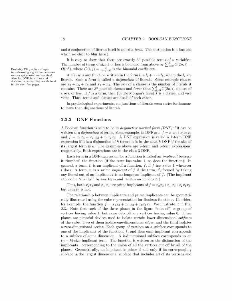
The relationship between implicants and prime implicants can be geometri-cally illustrated using the cube representation for Boolean functions. Consider,for example, the function f = x2x3 + x1 x3 + x2x1x3. We illustrate it in Fig.2.3. Note that each of the three planes in the figure “cuts off” a group ofvertices having value 1, but none cuts off any vertices having value 0. Theseplanes are pictorial devices used to isolate certain lower dimensional subfacesof the cube. Two of them isolate one-dimensional edges, and the third isolatesa zero-dimensional vertex. Each group of vertices on a subface corresponds toone of the implicants of the function, f , and thus each implicant correspondsto a subface of some dimension. A k-dimensional subface corresponds to an(n − k)-size implicant term. The function is written as the disjunction of theimplicants—corresponding to the union of all the vertices cut off by all of theplanes. Geometrically, an implicant is prime if and only if its correspondingsubface is the largest dimensional subface that includes all of its vertices and
2.2. CLASSES OF BOOLEAN FUNCTIONS 19
no other vertices having value 0. Note that the term x2x1x3 is not a primeimplicant of f . (In this case, we don’t even have to include this term in thefunction because the vertex cut off by the plane corresponding to x2x1x3 isalready cut off by the plane corresponding to x2x3.) The other two implicantsare prime because their corresponding subfaces cannot be expanded withoutincluding vertices having value 0.
x2
x1
x3
1, 0, 0
1, 0, 1
1, 1, 1
0, 0, 1
f = x2x3 + x1x3 + x2x1x3
= x2x3 + x1x3
x2x3 and x1x3 are prime implicants
Figure 2.3: A Function and its Implicants
Note that all Boolean functions can be represented in DNF—trivially bydisjunctions of terms of size n where each term corresponds to one of the verticeswhose value is 1. Whereas there are 22n functions of n dimensions in DNF (since
any Boolean function can be written in DNF), there are just 2O(nk) functionsin k-DNF.
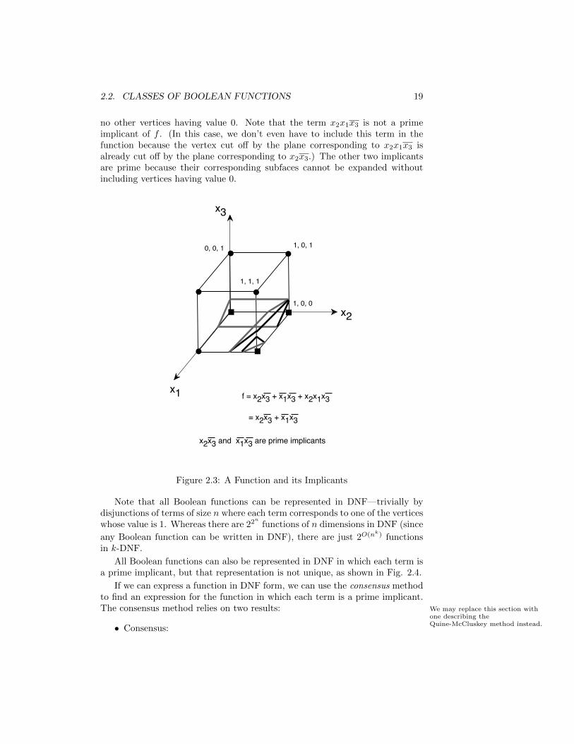
All Boolean functions can also be represented in DNF in which each term isa prime implicant, but that representation is not unique, as shown in Fig. 2.4.
If we can express a function in DNF form, we can use the consensus methodto find an expression for the function in which each term is a prime implicant.The consensus method relies on two results: We may replace this section with
one describing theQuine-McCluskey method instead.• Consensus:
20 CHAPTER 2. BOOLEAN FUNCTIONS
x2
x1
x3
1, 0, 0
1, 0, 1
1, 1, 1
0, 0, 1
f = x2x3 + x1x3 + x1x2
= x1x2 + x1x3
All of the terms are prime implicants, but thereis not a unique representation
Figure 2.4: Non-Uniqueness of Representation by Prime Implicants
xi · f1 + xi · f2 = xi · f1 + xi · f2 + f1 · f2
where f1 and f2 are terms such that no literal appearing in f1 appearscomplemented in f2. f1 · f2 is called the consensus of xi · f1 and xi ·f2. Readers familiar with the resolution rule of inference will note thatconsensus is the dual of resolution.
Examples: x1 is the consensus of x1x2 and x1x2. The terms x1x2 and x1x2
have no consensus since each term has more than one literal appearingcomplemented in the other.
• Subsumption:
xi · f1 + f1 = f1
where f1 is a term. We say that f1 subsumes xi · f1.
Example: x1 x4x5 subsumes x1 x4 x2x5
2.2. CLASSES OF BOOLEAN FUNCTIONS 21
The consensus method for finding a set of prime implicants for a function,f , iterates the following operations on the terms of a DNF expression for f untilno more such operations can be applied:
a. initialize the process with the set, T , of terms in the DNF expression off ,
b. compute the consensus of a pair of terms in T and add the result to T ,
c. eliminate any terms in T that are subsumed by other terms in T .
When this process halts, the terms remaining in T are all prime implicants off .
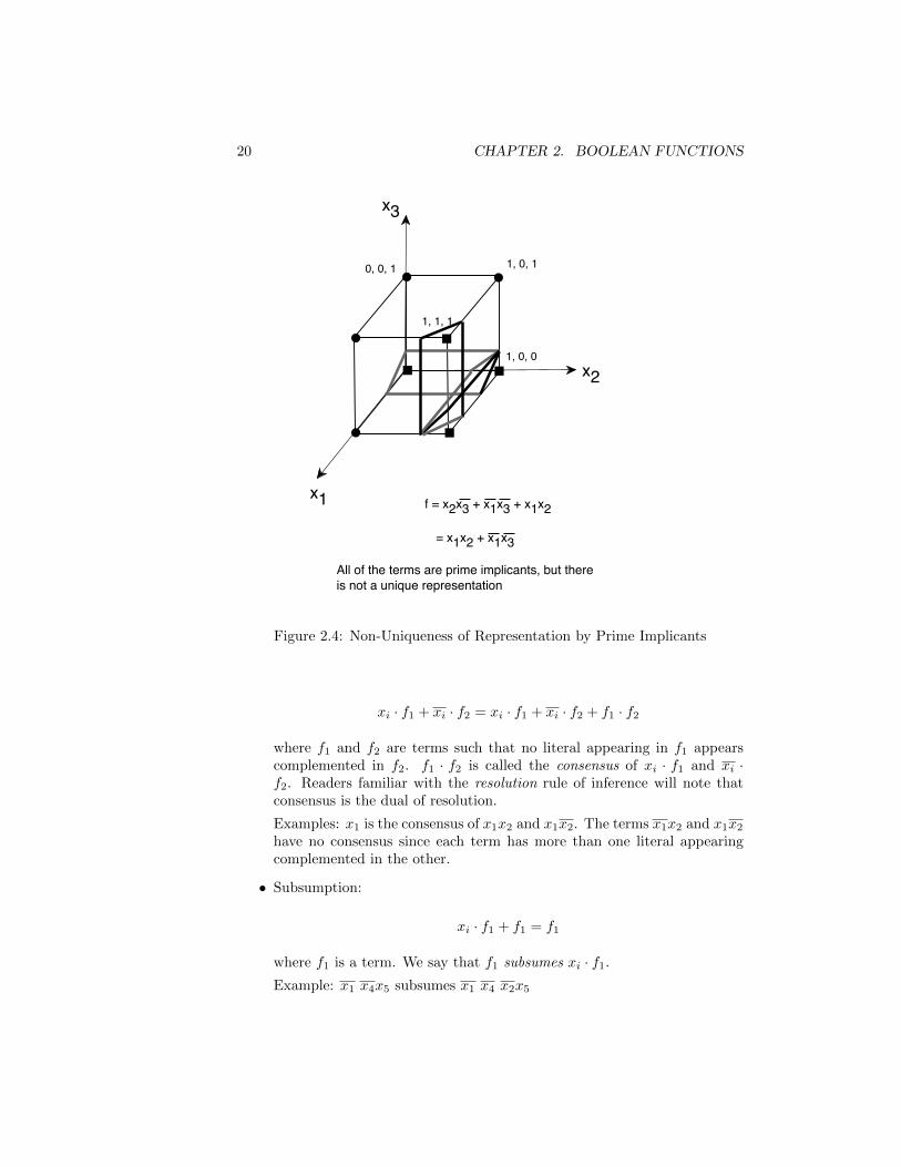
Example: Let f = x1x2 +x1 x2x3 +x1 x2 x3 x4x5. We show a derivation ofa set of prime implicants in the consensus tree of Fig. 2.5. The circled numbersadjoining the terms indicate the order in which the consensus and subsumptionoperations were performed. Shaded boxes surrounding a term indicate that itwas subsumed. The final form of the function in which all terms are primeimplicants is: f = x1x2 +x1x3 +x1 x4x5. Its terms are all of the non-subsumedterms in the consensus tree.
x1x2 x1x2x3 x1x2x3x4x5
x1x3
x1x2x4x5
x1x4x5
f = x1x2 + + x1x3 x1x4x5
1
2
6
4
5
3
Figure 2.5: A Consensus Tree
2.2.3 CNF Functions
Disjunctive normal form has a dual: conjunctive normal form (CNF). A Booleanfunction is said to be in CNF if it can be written as a conjunction of clauses.
22 CHAPTER 2. BOOLEAN FUNCTIONS
An example in CNF is: f = (x1 +x2)(x2 +x3 +x4). A CNF expression is calleda k-clause CNF expression if it is a conjunction of k clauses; it is in the classk-CNF if the size of its largest clause is k. The example is a 2-clause expressionin 3-CNF. If f is written in DNF, an application of De Morgan’s law renders f
in CNF, and vice versa. Because CNF and DNF are duals, there are also 2O(nk)
functions in k-CNF.
2.2.4 Decision Lists
Rivest has proposed a class of Boolean functions called decision lists [Rivest, 1987].A decision list is written as an ordered list of pairs:
(tq, vq)
(tq−1, vq−1)
· · ·
(ti, vi)
· · ·
(t2, v2)
(T, v1)
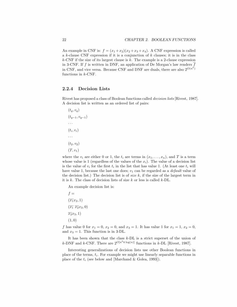
where the vi are either 0 or 1, the ti are terms in (x1, . . . , xn), and T is a termwhose value is 1 (regardless of the values of the xi). The value of a decision listis the value of vi for the first ti in the list that has value 1. (At least one ti willhave value 1, because the last one does; v1 can be regarded as a default value ofthe decision list.) The decision list is of size k, if the size of the largest term init is k. The class of decision lists of size k or less is called k-DL.
An example decision list is:
f =
(x1x2, 1)
(x1 x2x3, 0)
x2x3, 1)
(1, 0)
f has value 0 for x1 = 0, x2 = 0, and x3 = 1. It has value 1 for x1 = 1, x2 = 0,and x3 = 1. This function is in 3-DL.
It has been shown that the class k-DL is a strict superset of the union of
k-DNF and k-CNF. There are 2O[nkk log(n)] functions in k-DL [Rivest, 1987].
Interesting generalizations of decision lists use other Boolean functions inplace of the terms, ti. For example we might use linearly separable functions inplace of the ti (see below and [Marchand & Golea, 1993]).
2.2. CLASSES OF BOOLEAN FUNCTIONS 23
2.2.5 Symmetric and Voting Functions
A Boolean function is called symmetric if it is invariant under permutationsof the input variables. For example, any function that is dependent only onthe number of input variables whose values are 1 is a symmetric function. Theparity functions, which have value 1 depending on whether or not the numberof input variables with value 1 is even or odd is a symmetric function. (Theexclusive or function, illustrated in Fig. 2.1, is an odd-parity function of twodimensions. The or and and functions of two dimensions are also symmetric.)
An important subclass of the symmetric functions is the class of voting func-tions (also called m-of-n functions). A k-voting function has value 1 if and onlyif k or more of its n inputs has value 1. If k = 1, a voting function is the sameas an n-sized clause; if k = n, a voting function is the same as an n-sized term;if k = (n + 1)/2 for n odd or k = 1 + n/2 for n even, we have the majorityfunction.
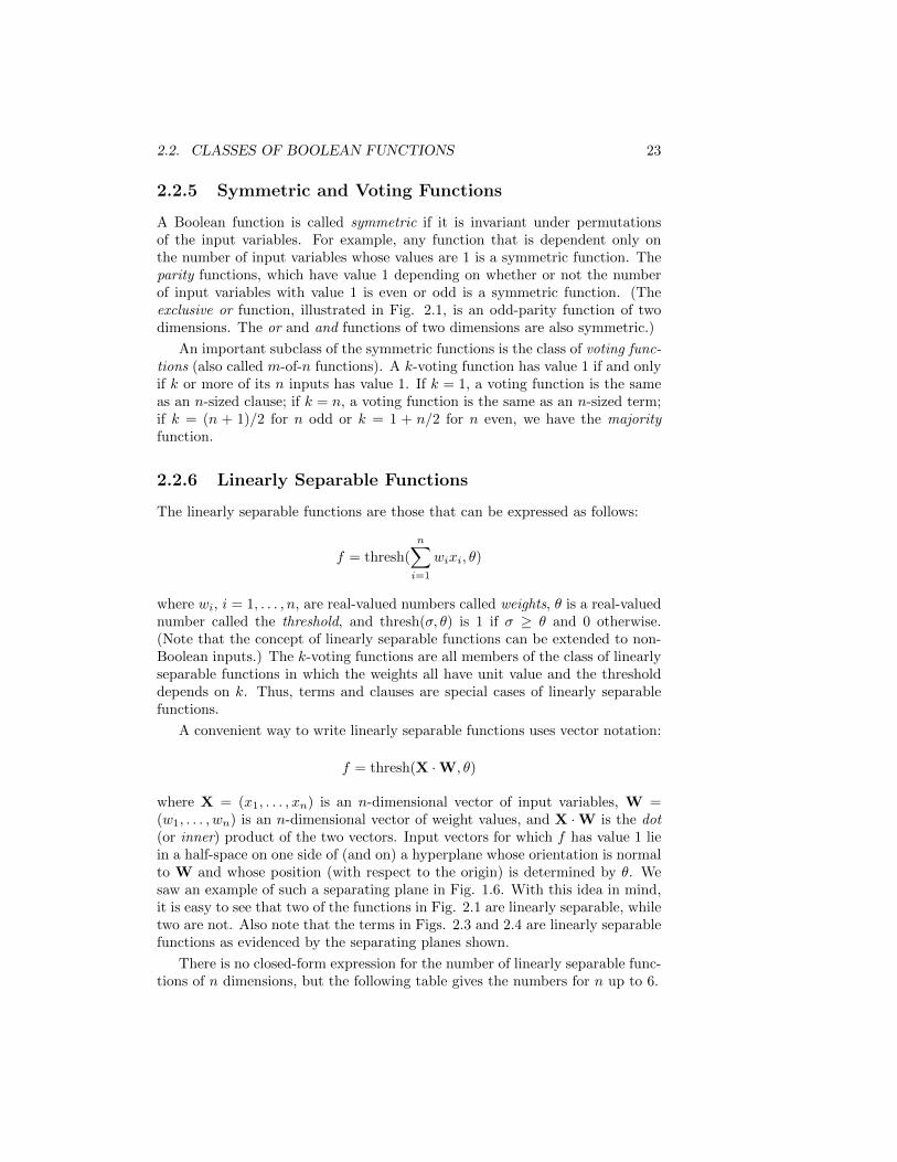
2.2.6 Linearly Separable Functions
The linearly separable functions are those that can be expressed as follows:
f = thresh(
n∑i=1
wixi, θ)
where wi, i = 1, . . . , n, are real-valued numbers called weights, θ is a real-valuednumber called the threshold, and thresh(σ, θ) is 1 if σ ≥ θ and 0 otherwise.(Note that the concept of linearly separable functions can be extended to non-Boolean inputs.) The k-voting functions are all members of the class of linearlyseparable functions in which the weights all have unit value and the thresholddepends on k. Thus, terms and clauses are special cases of linearly separablefunctions.
A convenient way to write linearly separable functions uses vector notation:
f = thresh(X ·W, θ)
where X = (x1, . . . , xn) is an n-dimensional vector of input variables, W =(w1, . . . , wn) is an n-dimensional vector of weight values, and X ·W is the dot(or inner) product of the two vectors. Input vectors for which f has value 1 liein a half-space on one side of (and on) a hyperplane whose orientation is normalto W and whose position (with respect to the origin) is determined by θ. Wesaw an example of such a separating plane in Fig. 1.6. With this idea in mind,it is easy to see that two of the functions in Fig. 2.1 are linearly separable, whiletwo are not. Also note that the terms in Figs. 2.3 and 2.4 are linearly separablefunctions as evidenced by the separating planes shown.
There is no closed-form expression for the number of linearly separable func-tions of n dimensions, but the following table gives the numbers for n up to 6.
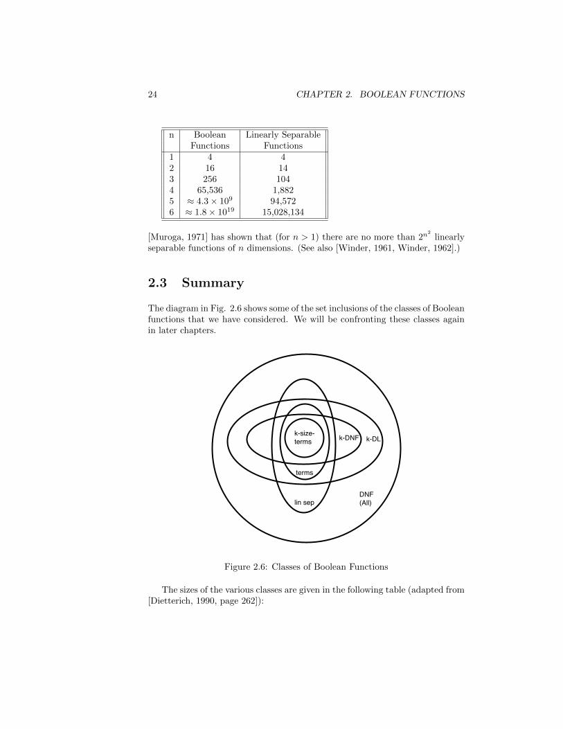
24 CHAPTER 2. BOOLEAN FUNCTIONS
n Boolean Linearly SeparableFunctions Functions
1 4 42 16 143 256 1044 65,536 1,8825 ≈ 4.3× 10⁹ 94,5726 ≈ 1.8× 10¹⁹ 15,028,134
[Muroga, 1971] has shown that (for n > 1) there are no more than 2n2
linearlyseparable functions of n dimensions. (See also [Winder, 1961, Winder, 1962].)
2.3 Summary
The diagram in Fig. 2.6 shows some of the set inclusions of the classes of Booleanfunctions that we have considered. We will be confronting these classes againin later chapters.
DNF(All)
k-DLk-DNFk-size-terms
terms
lin sep
Figure 2.6: Classes of Boolean Functions
The sizes of the various classes are given in the following table (adapted from[Dietterich, 1990, page 262]):

2.4. BIBLIOGRAPHICAL AND HISTORICAL REMARKS 25
Class Size of Classterms 3n
clauses 3n
k-term DNF 2O(kn)
k-clause CNF 2O(kn)
k-DNF 2O(nk)
k-CNF 2O(nk)
k-DL 2O[nkk log(n)]
lin sep 2O(n2)
DNF 22n
2.4 Bibliographical and Historical RemarksTo be added.

26 CHAPTER 2. BOOLEAN FUNCTIONS
Chapter 3
Using Version Spaces forLearning
3.1 Version Spaces and Mistake Bounds
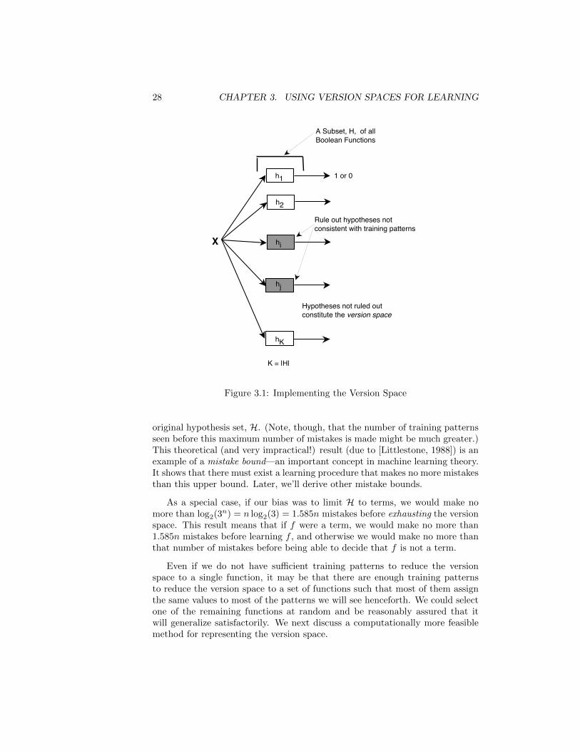
The first learning methods we present are based on the concepts of versionspaces and version graphs. These ideas are most clearly explained for the caseof Boolean function learning. Given an initial hypothesis set H (a subset ofall Boolean functions) and the values of f(X) for each X in a training set, Ξ,the version space is that subset of hypotheses, Hv, that is consistent with thesevalues. A hypothesis, h, is consistent with the values of X in Ξ if and only ifh(X) = f(X) for all X in Ξ. We say that the hypotheses in H that are notconsistent with the values in the training set are ruled out by the training set.
We could imagine (conceptually only!) that we have devices for implement-ing every function in H. An incremental training procedure could then bedefined which presented each pattern in Ξ to each of these functions and theneliminated those functions whose values for that pattern did not agree with itsgiven value. At any stage of the process we would then have left some subsetof functions that are consistent with the patterns presented so far; this subsetis the version space for the patterns already presented. This idea is illustratedin Fig. 3.1.
Consider the following procedure for classifying an arbitrary input pattern,X: the pattern is put in the same class (0 or 1) as are the majority of theoutputs of the functions in the version space. During the learning procedure,if this majority is not equal to the value of the pattern presented, we say amistake is made, and we revise the version space accordingly—eliminating allthose (majority of the) functions voting incorrectly. Thus, whenever a mistakeis made, we rule out at least half of the functions remaining in the version space.
How many mistakes can such a procedure make? Obviously, we can makeno more than log2(|H|) mistakes, where |H| is the number of hypotheses in the
27
28 CHAPTER 3. USING VERSION SPACES FOR LEARNING
h1
h2
hi
hK
X
A Subset, H, of allBoolean Functions
Rule out hypotheses notconsistent with training patterns
hj
Hypotheses not ruled outconstitute the version space
K = |H|
1 or 0
Figure 3.1: Implementing the Version Space
original hypothesis set, H. (Note, though, that the number of training patternsseen before this maximum number of mistakes is made might be much greater.)This theoretical (and very impractical!) result (due to [Littlestone, 1988]) is anexample of a mistake bound—an important concept in machine learning theory.It shows that there must exist a learning procedure that makes no more mistakesthan this upper bound. Later, we’ll derive other mistake bounds.
As a special case, if our bias was to limit H to terms, we would make nomore than log2(3n) = n log2(3) = 1.585n mistakes before exhausting the versionspace. This result means that if f were a term, we would make no more than1.585n mistakes before learning f , and otherwise we would make no more thanthat number of mistakes before being able to decide that f is not a term.
Even if we do not have sufficient training patterns to reduce the versionspace to a single function, it may be that there are enough training patternsto reduce the version space to a set of functions such that most of them assignthe same values to most of the patterns we will see henceforth. We could selectone of the remaining functions at random and be reasonably assured that itwill generalize satisfactorily. We next discuss a computationally more feasiblemethod for representing the version space.
3.2. VERSION GRAPHS 29
3.2 Version Graphs
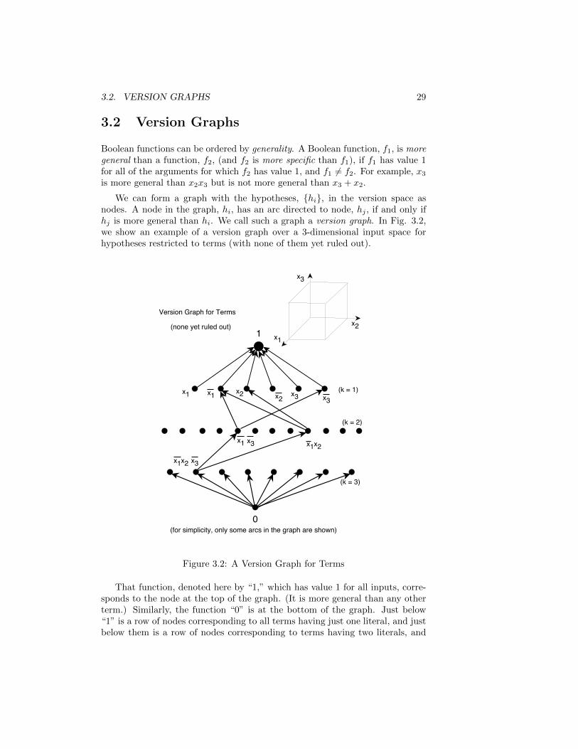
Boolean functions can be ordered by generality. A Boolean function, f1, is moregeneral than a function, f2, (and f2 is more specific than f1), if f1 has value 1for all of the arguments for which f2 has value 1, and f1 6= f2. For example, x3
is more general than x2x3 but is not more general than x3 + x2.
We can form a graph with the hypotheses, hi, in the version space asnodes. A node in the graph, hi, has an arc directed to node, hj , if and only ifhj is more general than hi. We call such a graph a version graph. In Fig. 3.2,we show an example of a version graph over a 3-dimensional input space forhypotheses restricted to terms (with none of them yet ruled out).
0
x1 x2 x3x2 x3
1
x1x2 x3
x1x2
x1
Version Graph for Terms
x1
x2
x3
(for simplicity, only some arcs in the graph are shown)
(none yet ruled out)
(k = 1)
(k = 2)
(k = 3)
x1 x3
Figure 3.2: A Version Graph for Terms
That function, denoted here by “1,” which has value 1 for all inputs, corre-sponds to the node at the top of the graph. (It is more general than any otherterm.) Similarly, the function “0” is at the bottom of the graph. Just below“1” is a row of nodes corresponding to all terms having just one literal, and justbelow them is a row of nodes corresponding to terms having two literals, and
30 CHAPTER 3. USING VERSION SPACES FOR LEARNING
so on. There are 33 = 27 functions altogether (the function “0,” included inthe graph, is technically not a term). To make our portrayal of the graph lesscluttered only some of the arcs are shown; each node in the actual graph has anarc directed to all of the nodes above it that are more general.
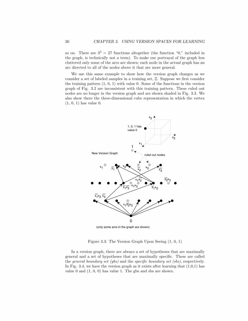
We use this same example to show how the version graph changes as weconsider a set of labeled samples in a training set, Ξ. Suppose we first considerthe training pattern (1, 0, 1) with value 0. Some of the functions in the versiongraph of Fig. 3.2 are inconsistent with this training pattern. These ruled outnodes are no longer in the version graph and are shown shaded in Fig. 3.3. Wealso show there the three-dimensional cube representation in which the vertex(1, 0, 1) has value 0.
0
x1 x2 x3x2 x3
1
x1x2 x3
x1x2
x1
New Version Graph
1, 0, 1 hasvalue 0
x1x3
x1x2 x2x3
x1x2x3
x1
x2
x3
x1x3
(only some arcs in the graph are shown)
ruled out nodes
Figure 3.3: The Version Graph Upon Seeing (1, 0, 1)
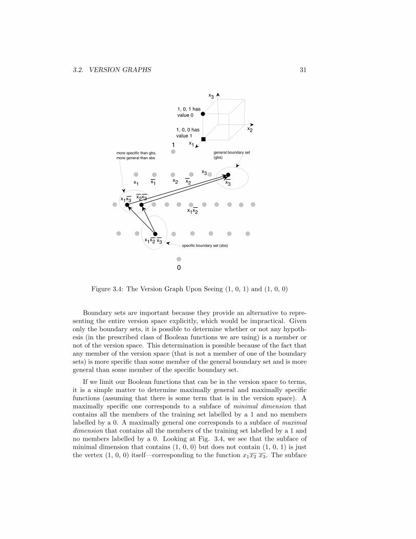
In a version graph, there are always a set of hypotheses that are maximallygeneral and a set of hypotheses that are maximally specific. These are calledthe general boundary set (gbs) and the specific boundary set (sbs), respectively.In Fig. 3.4, we have the version graph as it exists after learning that (1,0,1) hasvalue 0 and (1, 0, 0) has value 1. The gbs and sbs are shown.
3.2. VERSION GRAPHS 31
0
x1x2
x3x2 x3
1
x1x2 x3
x1
x2x3x1x3
general boundary set(gbs)
specific boundary set (sbs)
x1x2
more specific than gbs,more general than sbs
1, 0, 1 hasvalue 0
x1
x2
x3
1, 0, 0 hasvalue 1
Figure 3.4: The Version Graph Upon Seeing (1, 0, 1) and (1, 0, 0)
Boundary sets are important because they provide an alternative to repre-senting the entire version space explicitly, which would be impractical. Givenonly the boundary sets, it is possible to determine whether or not any hypoth-esis (in the prescribed class of Boolean functions we are using) is a member ornot of the version space. This determination is possible because of the fact thatany member of the version space (that is not a member of one of the boundarysets) is more specific than some member of the general boundary set and is moregeneral than some member of the specific boundary set.
If we limit our Boolean functions that can be in the version space to terms,it is a simple matter to determine maximally general and maximally specificfunctions (assuming that there is some term that is in the version space). Amaximally specific one corresponds to a subface of minimal dimension thatcontains all the members of the training set labelled by a 1 and no memberslabelled by a 0. A maximally general one corresponds to a subface of maximaldimension that contains all the members of the training set labelled by a 1 andno members labelled by a 0. Looking at Fig. 3.4, we see that the subface ofminimal dimension that contains (1, 0, 0) but does not contain (1, 0, 1) is justthe vertex (1, 0, 0) itself—corresponding to the function x1x2 x3. The subface
32 CHAPTER 3. USING VERSION SPACES FOR LEARNING
of maximal dimension that contains (1, 0, 0) but does not contain (1, 0, 1) isthe bottom face of the cube—corresponding to the function x3. In Figs. 3.2through 3.4 the sbs is always singular. Version spaces for terms always havesingular specific boundary sets. As seen in Fig. 3.3, however, the gbs of aversion space for terms need not be singular.
3.3 Learning as Search of a Version Space
[To be written. Relate to term learning algorithm presented in ChapterTwo. Also discuss best-first search methods. See Pat Langley’s example us-ing “pseudo-cells” of how to generate and eliminate hypotheses.]
Selecting a hypothesis from the version space can be thought of as a searchproblem. One can start with a very general function and specialize it throughvarious specialization operators until one finds a function that is consistent (oradequately so) with a set of training patterns. Such procedures are usuallycalled top-down methods. Or, one can start with a very special function andgeneralize it—resulting in bottom-up methods. We shall see instances of bothstyles of learning in this book.Compare this view of top-down
versus bottom-up with thedivide-and-conquer and thecovering (or AQ) methods ofdecision-tree induction. 3.4 The Candidate Elimination Method
The candidate elimination method, is an incremental method for computing theboundary sets. Quoting from [Hirsh, 1994, page 6]:
“The candidate-elimination algorithm manipulates the boundary-setrepresentation of a version space to create boundary sets that rep-resent a new version space consistent with all the previous instancesplus the new one. For a positive exmple the algorithm generalizesthe elements of the [sbs] as little as possible so that they cover thenew instance yet remain consistent with past data, and removesthose elements of the [gbs] that do not cover the new instance. Fora negative instance the algorithm specializes elements of the [gbs]so that they no longer cover the new instance yet remain consis-tent with past data, and removes from the [sbs] those elements thatmistakenly cover the new, negative instance.”
The method uses the following definitions (adapted from[Genesereth & Nilsson, 1987]):
• a hypothesis is called sufficient if and only if it has value 1 for all trainingsamples labeled by a 1,
• a hypothesis is called necessary if and only if it has value 0 for all trainingsamples labeled by a 0.
3.4. THE CANDIDATE ELIMINATION METHOD 33
Here is how to think about these definitions: A hypothesis implements a suffi-cient condition that a training sample has value 1 if the hypothesis has value 1for all of the positive instances; a hypothesis implements a necessary conditionthat a training sample has value 1 if the hypothesis has value 0 for all of thenegative instances. A hypothesis is consistent with the training set (and thus isin the version space) if and only if it is both sufficient and necessary.
We start (before receiving any members of the training set) with the function“0” as the singleton element of the specific boundary set and with the function“1” as the singleton element of the general boundary set. Upon receiving a newlabeled input vector, the boundary sets are changed as follows:
a. If the new vector is labelled with a 1:
The new general boundary set is obtained from the previous one by ex-cluding any elements in it that are not sufficient. (That is, we exclude anyelements that have value 0 for the new vector.)
The new specific boundary set is obtained from the previous one by re-placing each element, hi, in it by all of its least generalizations.
The hypothesis hg is a least generalization of h if and only if: a) h ismore specific than hg, b) hg is sufficient, c) no function (including h) thatis more specific than hg is sufficient, and d) hg is more specific than somemember of the new general boundary set. It might be that hg = h. Also,least generalizations of two different functions in the specific boundary setmay be identical.
b. If the new vector is labelled with a 0:
The new specific boundary set is obtained from the previous one by ex-cluding any elements in it that are not necessary. (That is, we excludeany elements that have value 1 for the new vector.)
The new general boundary set is obtained from the previous one by re-placing each element, hi, in it by all of its least specializations.
The hypothesis hs is a least specialization of h if and only if: a) h is moregeneral than hs, b) hs is necessary, c) no function (including h) that ismore general than hs is necessary, and d) hs is more general than somemember of the new specific boundary set. Again, it might be that hs = h,and least specializations of two different functions in the general boundaryset may be identical.
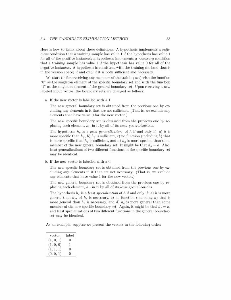
As an example, suppose we present the vectors in the following order:
vector label(1, 0, 1) 0(1, 0, 0) 1(1, 1, 1) 0(0, 0, 1) 0
34 CHAPTER 3. USING VERSION SPACES FOR LEARNING
We start with general boundary set, “1”, and specific boundary set, “0.”After seeing the first sample, (1, 0, 1), labeled with a 0, the specific boundaryset stays at “0” (it is necessary), and we change the general boundary set tox1, x2, x3. Each of the functions, x1, x2, and x3, are least specializations of“1” (they are necessary, “1” is not, they are more general than “0”, and thereare no functions that are more general than they and also necessary).
Then, after seeing (1, 0, 0), labeled with a 1, the general boundary setchanges to x3 (because x1 and x2 are not sufficient), and the specific boundaryset is changed to x1x2 x3. This single function is a least generalization of “0”(it is sufficient, “0” is more specific than it, no function (including “0”) that ismore specific than it is sufficient, and it is more specific than some member ofthe general boundary set.
When we see (1, 1, 1), labeled with a 0, we do not change the specificboundary set because its function is still necessary. We do not change thegeneral boundary set either because x3 is still necessary.
Finally, when we see (0, 0, 1), labeled with a 0, we do not change the specificboundary set because its function is still necessary. We do not change the generalboundary set either because x3 is still necessary.Maybe I’ll put in an example of a
version graph for non-Booleanfunctions.
3.5 Bibliographical and Historical Remarks
The concept of version spaces and their role in learning was first investigatedby Tom Mitchell [Mitchell, 1982]. Although these ideas are not used in prac-tical machine learning procedures, they do provide insight into the nature ofhypothesis selection. In order to accomodate noisy data, version spaces havebeen generalized by [Hirsh, 1994] to allow hypotheses that are not necessarilyconsistent with the training set.More to be added.
Chapter 4
Neural Networks
In chapter two we defined several important subsets of Boolean functions. Sup-pose we decide to use one of these subsets as a hypothesis set for supervisedfunction learning. We next have the question of how best to implement thefunction as a device that gives the outputs prescribed by the function for arbi-trary inputs. In this chapter we describe how networks of non-linear elementscan be used to implement various input-output functions and how they can betrained using supervised learning methods.
Networks of non-linear elements, interconnected through adjustable weights,play a prominent role in machine learning. They are called neural networks be-cause the non-linear elements have as their inputs a weighted sum of the outputsof other elements—much like networks of biological neurons do. These networkscommonly use the threshold element which we encountered in chapter two inour study of linearly separable Boolean functions. We begin our treatment ofneural nets by studying this threshold element and how it can be used in thesimplest of all networks, namely ones composed of a single threshold element.
4.1 Threshold Logic Units
4.1.1 Definitions and Geometry
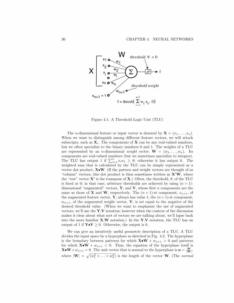
Linearly separable (threshold) functions are implemented in a straightforwardway by summing the weighted inputs and comparing this sum to a thresholdvalue as shown in Fig. 4.1. This structure we call a threshold logic unit (TLU).Its output is 1 or 0 depending on whether or not the weighted sum of its inputs isgreater than or equal to a threshold value, θ. It has also been called an Adaline(for adaptive linear element) [Widrow, 1962, Widrow & Lehr, 1990], an LTU(linear threshold unit), a perceptron, and a neuron. (Although the word “per-ceptron” is often used nowadays to refer to a single TLU, Rosenblatt originallydefined it as a class of networks of threshold elements [Rosenblatt, 1958].)
35
36 CHAPTER 4. NEURAL NETWORKS
!
x1x2
xn+1 = 1
xi
w1w2
wn+1
wi
wn
X
threshold weightxn
W threshold " = 0
f
f = thresh( ! wi xi, 0)i = 1
n+1
Figure 4.1: A Threshold Logic Unit (TLU)
The n-dimensional feature or input vector is denoted by X = (x1, . . . , xn).When we want to distinguish among different feature vectors, we will attachsubscripts, such as Xi. The components of X can be any real-valued numbers,but we often specialize to the binary numbers 0 and 1. The weights of a TLUare represented by an n-dimensional weight vector, W = (w1, . . . , wn). Itscomponents are real-valued numbers (but we sometimes specialize to integers).The TLU has output 1 if
∑ni=1 xiwi ≥ θ; otherwise it has output 0. The
weighted sum that is calculated by the TLU can be simply represented as avector dot product, X•W. (If the pattern and weight vectors are thought of as“column” vectors, this dot product is then sometimes written as XtW, wherethe “row” vector Xt is the transpose of X.) Often, the threshold, θ, of the TLUis fixed at 0; in that case, arbitrary thresholds are achieved by using (n + 1)-dimensional “augmented” vectors, Y, and V, whose first n components are thesame as those of X and W, respectively. The (n + 1)-st component, xn+1, ofthe augmented feature vector, Y, always has value 1; the (n+ 1)-st component,wn+1, of the augmented weight vector, V, is set equal to the negative of thedesired threshold value. (When we want to emphasize the use of augmentedvectors, we’ll use the Y,V notation; however when the context of the discussionmakes it clear about what sort of vectors we are talking about, we’ll lapse backinto the more familiar X,W notation.) In the Y,V notation, the TLU has anoutput of 1 if Y•V ≥ 0. Otherwise, the output is 0.
We can give an intuitively useful geometric description of a TLU. A TLUdivides the input space by a hyperplane as sketched in Fig. 4.2. The hyperplaneis the boundary between patterns for which X•W + wn+1 > 0 and patternsfor which X•W + wn+1 < 0. Thus, the equation of the hyperplane itself isX•W+wn+1 = 0. The unit vector that is normal to the hyperplane is n = W
|W| ,
where |W| =√
(w21 + . . .+ w2
n) is the length of the vector W. (The normal
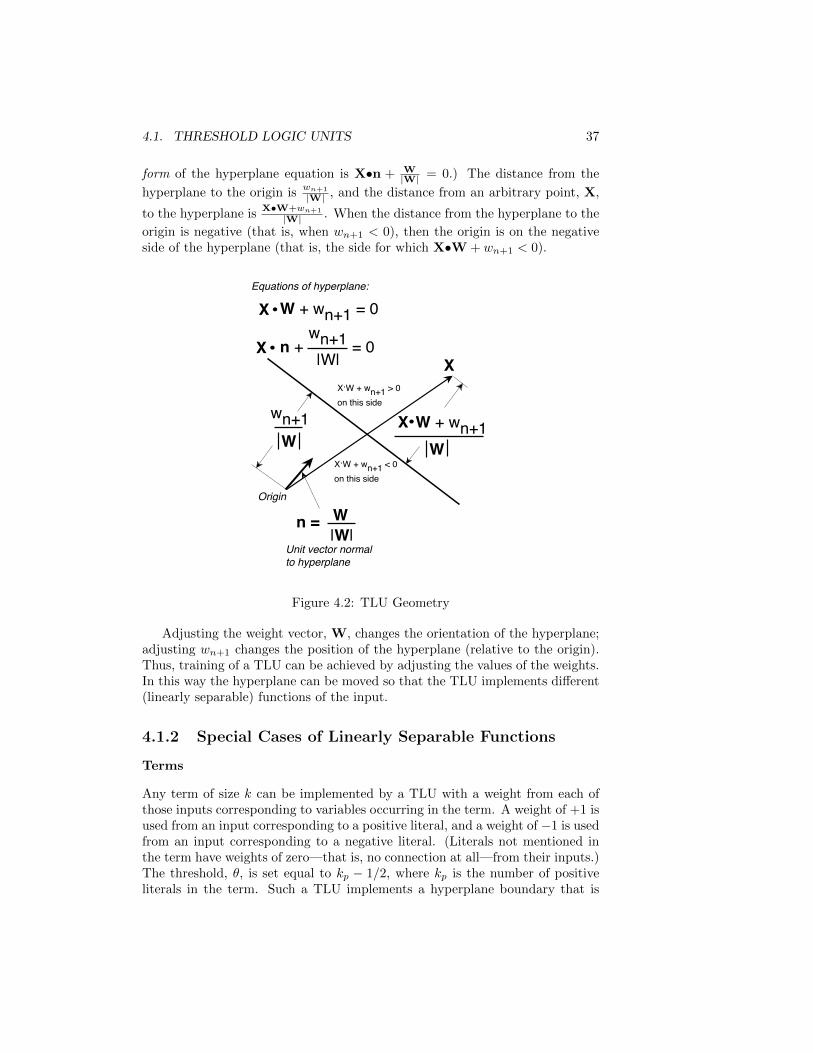
4.1. THRESHOLD LOGIC UNITS 37
form of the hyperplane equation is X•n + W|W| = 0.) The distance from the
hyperplane to the origin is wn+1
|W| , and the distance from an arbitrary point, X,
to the hyperplane is X•W+wn+1
|W| . When the distance from the hyperplane to the
origin is negative (that is, when wn+1 < 0), then the origin is on the negativeside of the hyperplane (that is, the side for which X•W + wn+1 < 0).
X.W + wn+1 > 0on this side
W
X
W
n = W|W|
Origin
Unit vector normalto hyperplane
W + wn+1 = 0X
n + = 0X
Equations of hyperplane:
wn+1|W|
wn+1 W + wn+1X
X.W + wn+1 < 0on this side
Figure 4.2: TLU Geometry
Adjusting the weight vector, W, changes the orientation of the hyperplane;adjusting wn+1 changes the position of the hyperplane (relative to the origin).Thus, training of a TLU can be achieved by adjusting the values of the weights.In this way the hyperplane can be moved so that the TLU implements different(linearly separable) functions of the input.
4.1.2 Special Cases of Linearly Separable Functions
Terms
Any term of size k can be implemented by a TLU with a weight from each ofthose inputs corresponding to variables occurring in the term. A weight of +1 isused from an input corresponding to a positive literal, and a weight of −1 is usedfrom an input corresponding to a negative literal. (Literals not mentioned inthe term have weights of zero—that is, no connection at all—from their inputs.)The threshold, θ, is set equal to kp − 1/2, where kp is the number of positiveliterals in the term. Such a TLU implements a hyperplane boundary that is
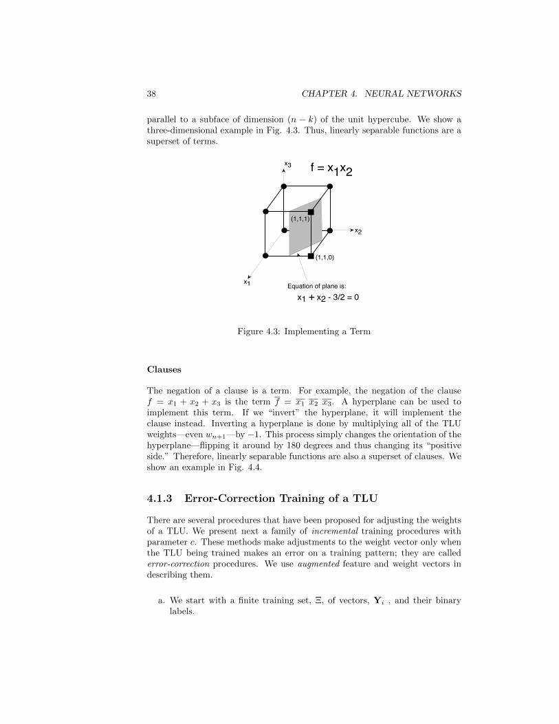
38 CHAPTER 4. NEURAL NETWORKS
parallel to a subface of dimension (n − k) of the unit hypercube. We show athree-dimensional example in Fig. 4.3. Thus, linearly separable functions are asuperset of terms.
(1,1,1)
(1,1,0)
x2
x1
x3 f = x1x2
x1 + x2 - 3/2 = 0Equation of plane is:
Figure 4.3: Implementing a Term
Clauses
The negation of a clause is a term. For example, the negation of the clausef = x1 + x2 + x3 is the term f = x1 x2 x3. A hyperplane can be used toimplement this term. If we “invert” the hyperplane, it will implement theclause instead. Inverting a hyperplane is done by multiplying all of the TLUweights—even wn+1—by −1. This process simply changes the orientation of thehyperplane—flipping it around by 180 degrees and thus changing its “positiveside.” Therefore, linearly separable functions are also a superset of clauses. Weshow an example in Fig. 4.4.
4.1.3 Error-Correction Training of a TLU
There are several procedures that have been proposed for adjusting the weightsof a TLU. We present next a family of incremental training procedures withparameter c. These methods make adjustments to the weight vector only whenthe TLU being trained makes an error on a training pattern; they are callederror-correction procedures. We use augmented feature and weight vectors indescribing them.
a. We start with a finite training set, Ξ, of vectors, Yi , and their binarylabels.
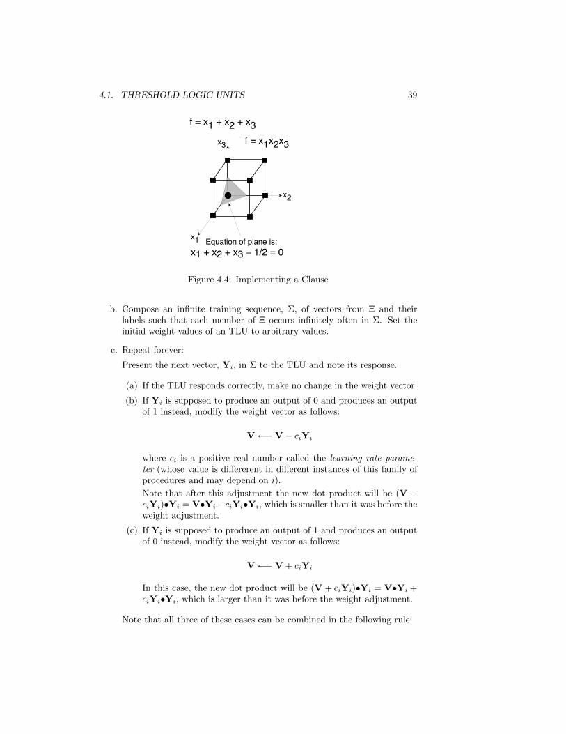
4.1. THRESHOLD LOGIC UNITS 39
f = x1 + x2 + x3
x1x1 + x2 + x3 1/2 = 0
f = x1x2x3
Equation of plane is:
x2
x3
Figure 4.4: Implementing a Clause
b. Compose an infinite training sequence, Σ, of vectors from Ξ and theirlabels such that each member of Ξ occurs infinitely often in Σ. Set theinitial weight values of an TLU to arbitrary values.
c. Repeat forever:
Present the next vector, Yi, in Σ to the TLU and note its response.
(a) If the TLU responds correctly, make no change in the weight vector.
(b) If Yi is supposed to produce an output of 0 and produces an outputof 1 instead, modify the weight vector as follows:
V←− V − ciYi
where ci is a positive real number called the learning rate parame-ter (whose value is differerent in different instances of this family ofprocedures and may depend on i).
Note that after this adjustment the new dot product will be (V −ciYi)•Yi = V•Yi−ciYi•Yi, which is smaller than it was before theweight adjustment.
(c) If Yi is supposed to produce an output of 1 and produces an outputof 0 instead, modify the weight vector as follows:
V←− V + ciYi
In this case, the new dot product will be (V + ciYi)•Yi = V•Yi +ciYi•Yi, which is larger than it was before the weight adjustment.
Note that all three of these cases can be combined in the following rule:
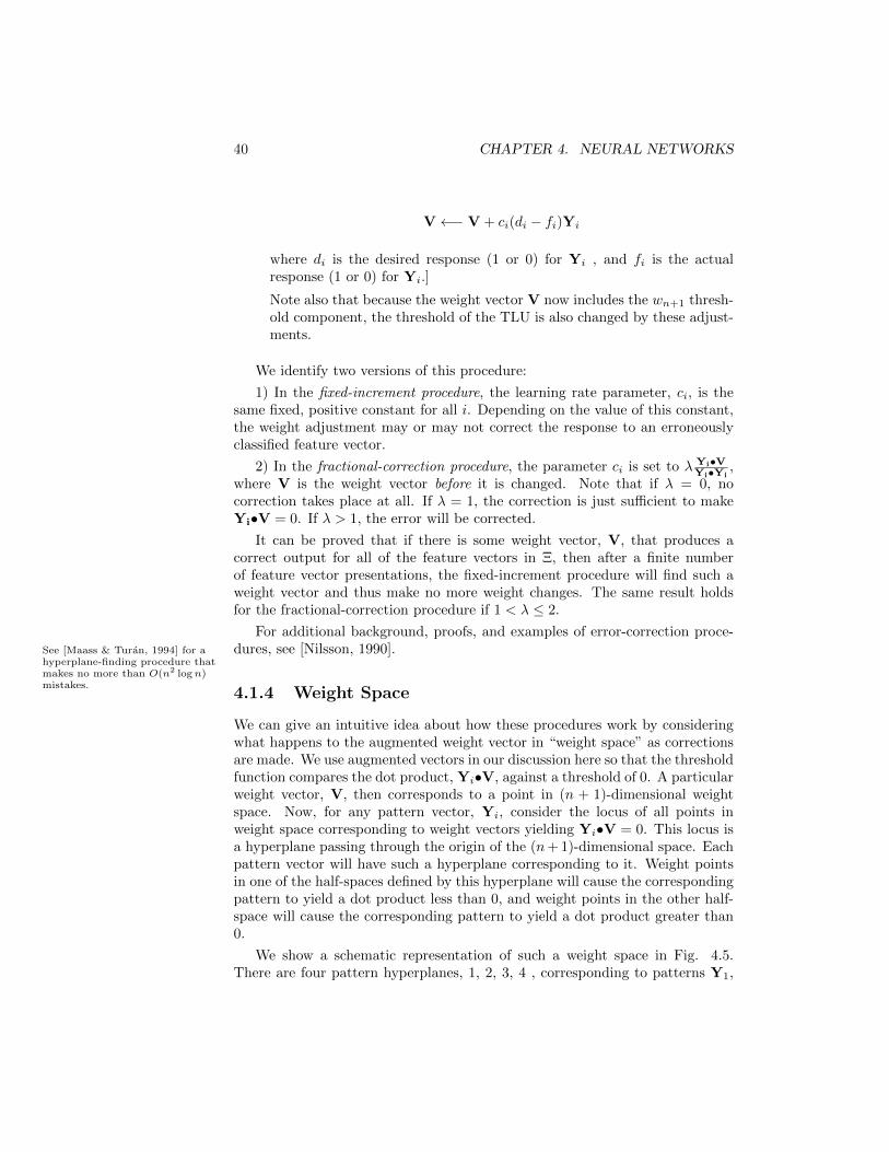
40 CHAPTER 4. NEURAL NETWORKS
V←− V + ci(di − fi)Yi
where di is the desired response (1 or 0) for Yi , and fi is the actualresponse (1 or 0) for Yi.]
Note also that because the weight vector V now includes the wn+1 thresh-old component, the threshold of the TLU is also changed by these adjust-ments.
We identify two versions of this procedure:
1) In the fixed-increment procedure, the learning rate parameter, ci, is thesame fixed, positive constant for all i. Depending on the value of this constant,the weight adjustment may or may not correct the response to an erroneouslyclassified feature vector.
2) In the fractional-correction procedure, the parameter ci is set to λ Yi•VYi•Yi
,where V is the weight vector before it is changed. Note that if λ = 0, nocorrection takes place at all. If λ = 1, the correction is just sufficient to makeYi•V = 0. If λ > 1, the error will be corrected.
It can be proved that if there is some weight vector, V, that produces acorrect output for all of the feature vectors in Ξ, then after a finite numberof feature vector presentations, the fixed-increment procedure will find such aweight vector and thus make no more weight changes. The same result holdsfor the fractional-correction procedure if 1 < λ ≤ 2.
For additional background, proofs, and examples of error-correction proce-dures, see [Nilsson, 1990].See [Maass & Turan, 1994] for a
hyperplane-finding procedure thatmakes no more than O(n2 logn)mistakes.
4.1.4 Weight Space
We can give an intuitive idea about how these procedures work by consideringwhat happens to the augmented weight vector in “weight space” as correctionsare made. We use augmented vectors in our discussion here so that the thresholdfunction compares the dot product, Yi•V, against a threshold of 0. A particularweight vector, V, then corresponds to a point in (n + 1)-dimensional weightspace. Now, for any pattern vector, Yi, consider the locus of all points inweight space corresponding to weight vectors yielding Yi•V = 0. This locus isa hyperplane passing through the origin of the (n+ 1)-dimensional space. Eachpattern vector will have such a hyperplane corresponding to it. Weight pointsin one of the half-spaces defined by this hyperplane will cause the correspondingpattern to yield a dot product less than 0, and weight points in the other half-space will cause the corresponding pattern to yield a dot product greater than0.
We show a schematic representation of such a weight space in Fig. 4.5.There are four pattern hyperplanes, 1, 2, 3, 4 , corresponding to patterns Y1,
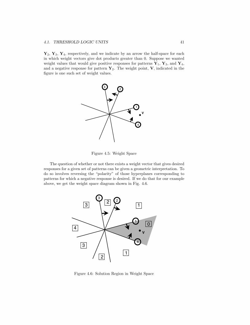
4.1. THRESHOLD LOGIC UNITS 41
Y2, Y3, Y4, respectively, and we indicate by an arrow the half-space for eachin which weight vectors give dot products greater than 0. Suppose we wantedweight values that would give positive responses for patterns Y1, Y3, and Y4,and a negative response for pattern Y2. The weight point, V, indicated in thefigure is one such set of weight values.
23
4
1
V
Figure 4.5: Weight Space
The question of whether or not there exists a weight vector that gives desiredresponses for a given set of patterns can be given a geometric interpretation. Todo so involves reversing the “polarity” of those hyperplanes corresponding topatterns for which a negative response is desired. If we do that for our exampleabove, we get the weight space diagram shown in Fig. 4.6.
23
4
1
V
0
1
1
23
2
3
4
Figure 4.6: Solution Region in Weight Space
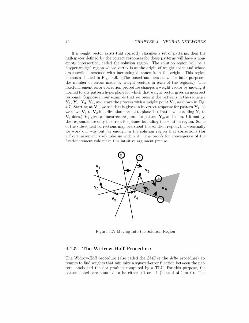
42 CHAPTER 4. NEURAL NETWORKS
If a weight vector exists that correctly classifies a set of patterns, then thehalf-spaces defined by the correct responses for these patterns will have a non-empty intersection, called the solution region. The solution region will be a“hyper-wedge” region whose vertex is at the origin of weight space and whosecross-section increases with increasing distance from the origin. This regionis shown shaded in Fig. 4.6. (The boxed numbers show, for later purposes,the number of errors made by weight vectors in each of the regions.) Thefixed-increment error-correction procedure changes a weight vector by moving itnormal to any pattern hyperplane for which that weight vector gives an incorrectresponse. Suppose in our example that we present the patterns in the sequenceY1, Y2, Y3, Y4, and start the process with a weight point V1, as shown in Fig.4.7. Starting at V1, we see that it gives an incorrect response for pattern Y1, sowe move V1 to V2 in a direction normal to plane 1. (That is what adding Y1 toV1 does.) Y2 gives an incorrect response for pattern Y2, and so on. Ultimately,the responses are only incorrect for planes bounding the solution region. Someof the subsequent corrections may overshoot the solution region, but eventuallywe work our way out far enough in the solution region that corrections (fora fixed increment size) take us within it. The proofs for convergence of thefixed-increment rule make this intuitive argument precise.
23
4
1
V
V1
V2
V3V4
V5
V6
Figure 4.7: Moving Into the Solution Region
4.1.5 The Widrow-Hoff Procedure
The Widrow-Hoff procedure (also called the LMS or the delta procedure) at-tempts to find weights that minimize a squared-error function between the pat-tern labels and the dot product computed by a TLU. For this purpose, thepattern labels are assumed to be either +1 or −1 (instead of 1 or 0). The
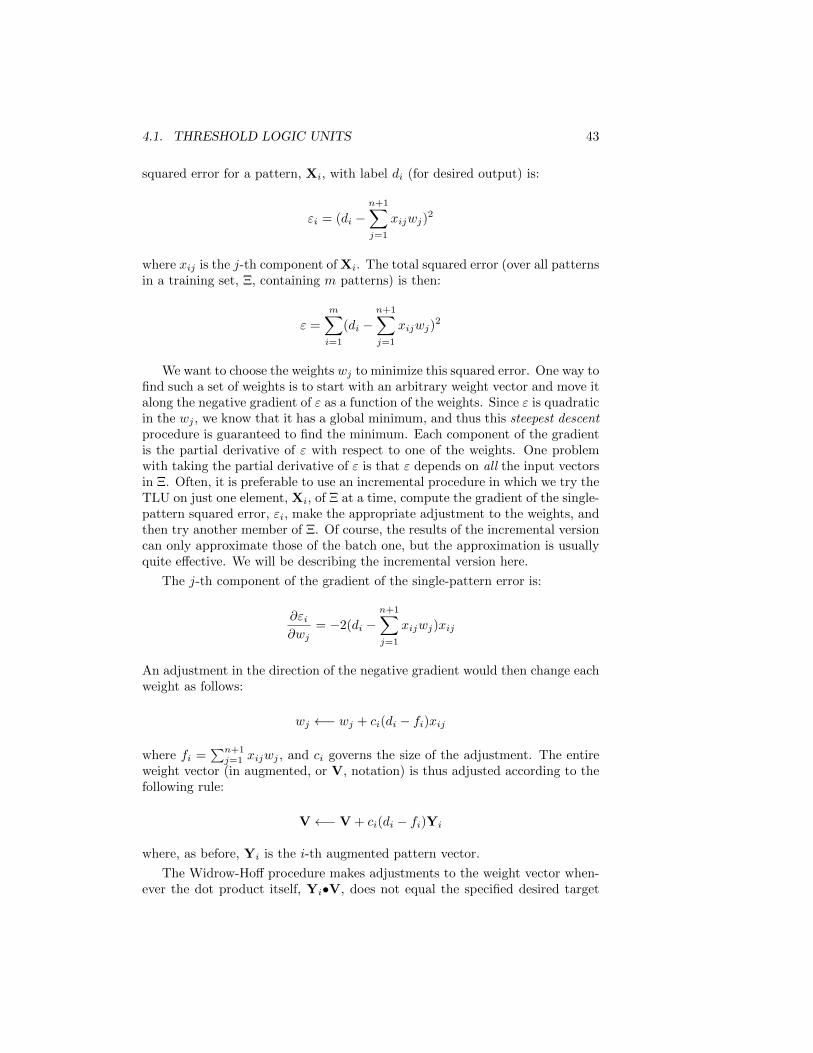
4.1. THRESHOLD LOGIC UNITS 43
squared error for a pattern, Xi, with label di (for desired output) is:
εi = (di −n+1∑j=1
xijwj)2
where xij is the j-th component of Xi. The total squared error (over all patternsin a training set, Ξ, containing m patterns) is then:
ε =
m∑i=1
(di −n+1∑j=1
xijwj)2
We want to choose the weights wj to minimize this squared error. One way tofind such a set of weights is to start with an arbitrary weight vector and move italong the negative gradient of ε as a function of the weights. Since ε is quadraticin the wj , we know that it has a global minimum, and thus this steepest descentprocedure is guaranteed to find the minimum. Each component of the gradientis the partial derivative of ε with respect to one of the weights. One problemwith taking the partial derivative of ε is that ε depends on all the input vectorsin Ξ. Often, it is preferable to use an incremental procedure in which we try theTLU on just one element, Xi, of Ξ at a time, compute the gradient of the single-pattern squared error, εi, make the appropriate adjustment to the weights, andthen try another member of Ξ. Of course, the results of the incremental versioncan only approximate those of the batch one, but the approximation is usuallyquite effective. We will be describing the incremental version here.
The j-th component of the gradient of the single-pattern error is:
∂εi∂wj
= −2(di −n+1∑j=1
xijwj)xij
An adjustment in the direction of the negative gradient would then change eachweight as follows:
wj ←− wj + ci(di − fi)xij
where fi =∑n+1j=1 xijwj , and ci governs the size of the adjustment. The entire
weight vector (in augmented, or V, notation) is thus adjusted according to thefollowing rule:
V←− V + ci(di − fi)Yi
where, as before, Yi is the i-th augmented pattern vector.
The Widrow-Hoff procedure makes adjustments to the weight vector when-ever the dot product itself, Yi•V, does not equal the specified desired target
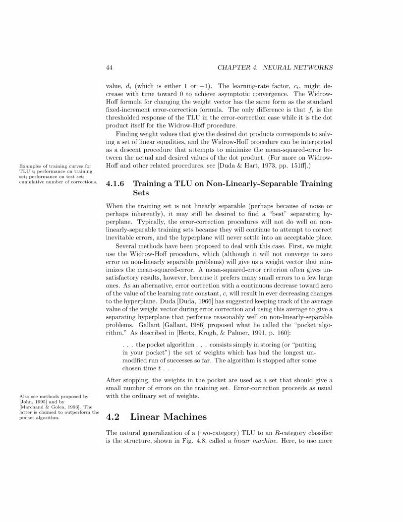
44 CHAPTER 4. NEURAL NETWORKS
value, di (which is either 1 or −1). The learning-rate factor, ci, might de-crease with time toward 0 to achieve asymptotic convergence. The Widrow-Hoff formula for changing the weight vector has the same form as the standardfixed-increment error-correction formula. The only difference is that fi is thethresholded response of the TLU in the error-correction case while it is the dotproduct itself for the Widrow-Hoff procedure.
Finding weight values that give the desired dot products corresponds to solv-ing a set of linear equalities, and the Widrow-Hoff procedure can be interpretedas a descent procedure that attempts to minimize the mean-squared-error be-tween the actual and desired values of the dot product. (For more on Widrow-Hoff and other related procedures, see [Duda & Hart, 1973, pp. 151ff].)Examples of training curves for
TLU’s; performance on trainingset; performance on test set;cumulative number of corrections. 4.1.6 Training a TLU on Non-Linearly-Separable Training
Sets
When the training set is not linearly separable (perhaps because of noise orperhaps inherently), it may still be desired to find a “best” separating hy-perplane. Typically, the error-correction procedures will not do well on non-linearly-separable training sets because they will continue to attempt to correctinevitable errors, and the hyperplane will never settle into an acceptable place.
Several methods have been proposed to deal with this case. First, we mightuse the Widrow-Hoff procedure, which (although it will not converge to zeroerror on non-linearly separable problems) will give us a weight vector that min-imizes the mean-squared-error. A mean-squared-error criterion often gives un-satisfactory results, however, because it prefers many small errors to a few largeones. As an alternative, error correction with a continuous decrease toward zeroof the value of the learning rate constant, c, will result in ever decreasing changesto the hyperplane. Duda [Duda, 1966] has suggested keeping track of the averagevalue of the weight vector during error correction and using this average to give aseparating hyperplane that performs reasonably well on non-linearly-separableproblems. Gallant [Gallant, 1986] proposed what he called the “pocket algo-rithm.” As described in [Hertz, Krogh, & Palmer, 1991, p. 160]:
. . . the pocket algorithm . . . consists simply in storing (or “puttingin your pocket”) the set of weights which has had the longest un-modified run of successes so far. The algorithm is stopped after somechosen time t . . .
After stopping, the weights in the pocket are used as a set that should give asmall number of errors on the training set. Error-correction proceeds as usualwith the ordinary set of weights.Also see methods proposed by
[John, 1995] and by[Marchand & Golea, 1993]. Thelatter is claimed to outperform thepocket algorithm. 4.2 Linear Machines
The natural generalization of a (two-category) TLU to an R-category classifieris the structure, shown in Fig. 4.8, called a linear machine. Here, to use more
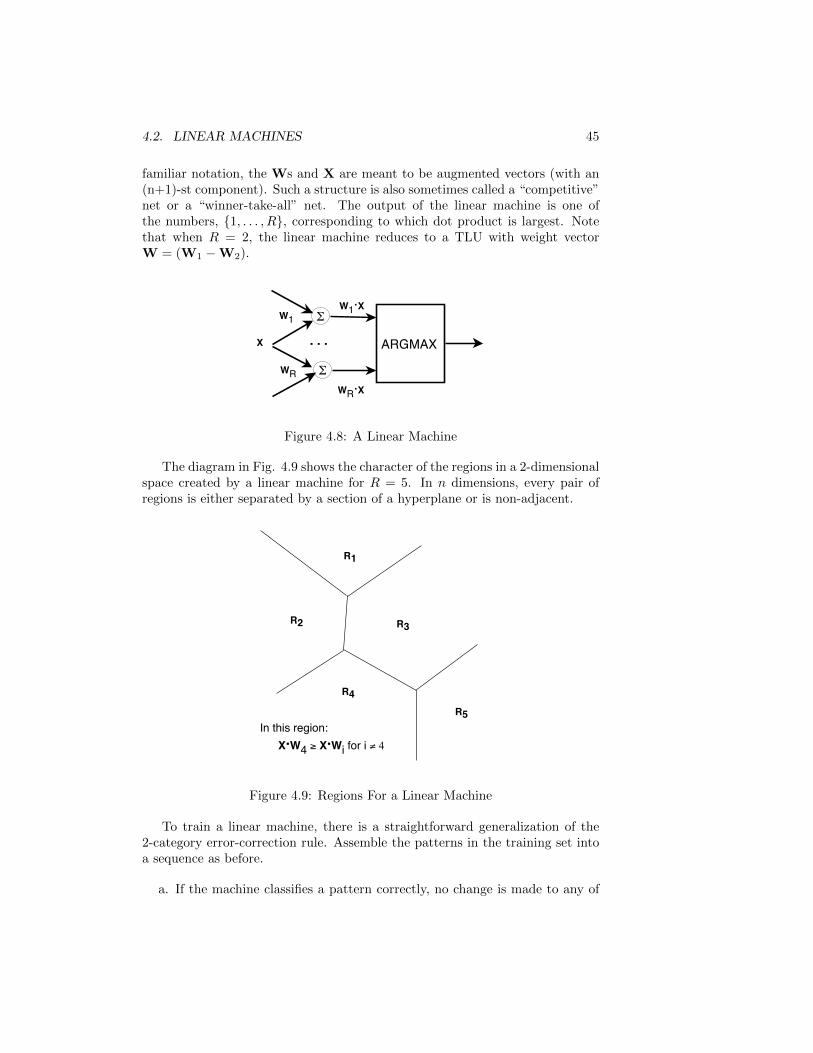
4.2. LINEAR MACHINES 45
familiar notation, the Ws and X are meant to be augmented vectors (with an(n+1)-st component). Such a structure is also sometimes called a “competitive”net or a “winner-take-all” net. The output of the linear machine is one ofthe numbers, 1, . . . , R, corresponding to which dot product is largest. Notethat when R = 2, the linear machine reduces to a TLU with weight vectorW = (W1 −W2).
X
W1
WR
. . . ARGMAX
W1.X
WR.X
Figure 4.8: A Linear Machine
The diagram in Fig. 4.9 shows the character of the regions in a 2-dimensionalspace created by a linear machine for R = 5. In n dimensions, every pair ofregions is either separated by a section of a hyperplane or is non-adjacent.
R1
R3
R4R5
X.W4 X.Wi for i 4
R2
In this region:
Figure 4.9: Regions For a Linear Machine
To train a linear machine, there is a straightforward generalization of the2-category error-correction rule. Assemble the patterns in the training set intoa sequence as before.
a. If the machine classifies a pattern correctly, no change is made to any of
46 CHAPTER 4. NEURAL NETWORKS
the weight vectors.
b. If the machine mistakenly classifies a category u pattern, Xi, in categoryv (u 6= v), then:
Wu ←−Wu + ciXi
and
Wv ←−Wv − ciXi
and all other weight vectors are not changed.
This correction increases the value of the u-th dot product and decreases thevalue of the v-th dot product. Just as in the 2-category fixed increment proce-dure, this procedure is guaranteed to terminate, for constant ci, if there existsweight vectors that make correct separations of the training set. Note that whenR = 2, this procedure reduces to the ordinary TLU error-correction procedure.A proof that this procedure terminates is given in [Nilsson, 1990, pp. 88-90]and in [Duda & Hart, 1973, pp. 174-177].
4.3 Networks of TLUs
4.3.1 Motivation and Examples
Layered Networks
To classify correctly all of the patterns in non-linearly-separable training sets re-quires separating surfaces more complex than hyperplanes. One way to achievemore complex surfaces is with networks of TLUs. Consider, for example, the 2-dimensional, even parity function, f = x1x2 +x1 x2. No single line through the2-dimensional square can separate the vertices (1,1) and (0,0) from the vertices(1,0) and (0,1)—the function is not linearly separable and thus cannot be im-plemented by a single TLU. But, the network of three TLUs shown in Fig. 4.10does implement this function. In the figure, we show the weight values alonginput lines to each TLU and the threshold value inside the circle representingthe TLU.
The function implemented by a network of TLUs depends on its topologyas well as on the weights of the individual TLUs. Feedforward networks haveno cycles; in a feedforward network no TLU’s input depends (through zeroor more intermediate TLUs) on that TLU’s output. (Networks that are notfeedforward are called recurrent networks). If the TLUs of a feedforward networkare arranged in layers, with the elements of layer j receiving inputs only fromTLUs in layer j − 1, then we say that the network is a layered, feedforward
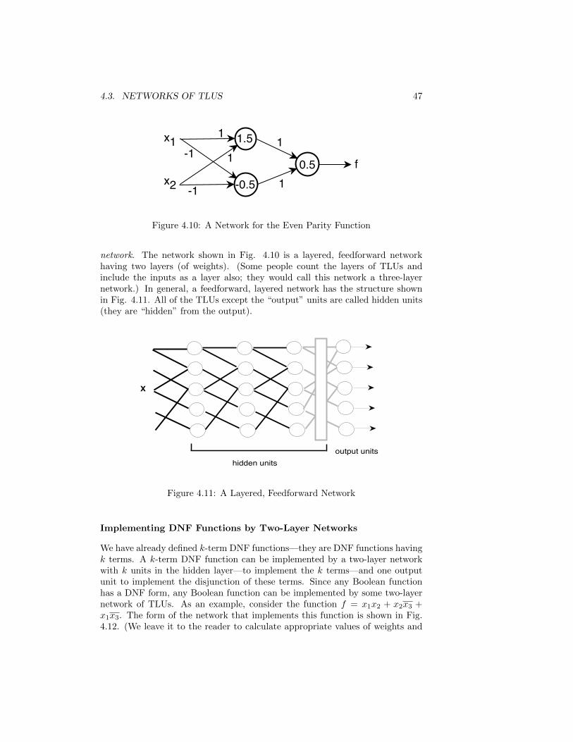
4.3. NETWORKS OF TLUS 47
f
x1
x2
1.5
-0.50.5
1
1-1
-1 1
1
Figure 4.10: A Network for the Even Parity Function
network. The network shown in Fig. 4.10 is a layered, feedforward networkhaving two layers (of weights). (Some people count the layers of TLUs andinclude the inputs as a layer also; they would call this network a three-layernetwork.) In general, a feedforward, layered network has the structure shownin Fig. 4.11. All of the TLUs except the “output” units are called hidden units(they are “hidden” from the output).
X
hidden unitsoutput units
Figure 4.11: A Layered, Feedforward Network
Implementing DNF Functions by Two-Layer Networks
We have already defined k-term DNF functions—they are DNF functions havingk terms. A k-term DNF function can be implemented by a two-layer networkwith k units in the hidden layer—to implement the k terms—and one outputunit to implement the disjunction of these terms. Since any Boolean functionhas a DNF form, any Boolean function can be implemented by some two-layernetwork of TLUs. As an example, consider the function f = x1x2 + x2x3 +x1x3. The form of the network that implements this function is shown in Fig.4.12. (We leave it to the reader to calculate appropriate values of weights and
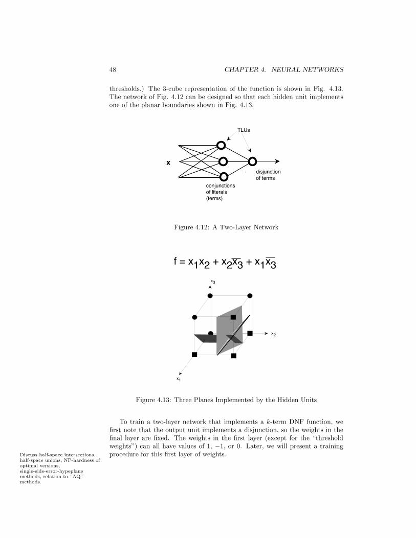
48 CHAPTER 4. NEURAL NETWORKS
thresholds.) The 3-cube representation of the function is shown in Fig. 4.13.The network of Fig. 4.12 can be designed so that each hidden unit implementsone of the planar boundaries shown in Fig. 4.13.
x
conjuncts
disjunct
A Feedforward, 2-layer Network
TLUs
disjunctionof terms
conjunctionsof literals(terms)
Figure 4.12: A Two-Layer Network
x2
x1
x3
f = x1x2 + x2x3 + x1x3
Figure 4.13: Three Planes Implemented by the Hidden Units
To train a two-layer network that implements a k-term DNF function, wefirst note that the output unit implements a disjunction, so the weights in thefinal layer are fixed. The weights in the first layer (except for the “thresholdweights”) can all have values of 1, −1, or 0. Later, we will present a trainingprocedure for this first layer of weights.Discuss half-space intersections,
half-space unions, NP-hardness ofoptimal versions,single-side-error-hypeplanemethods, relation to “AQ”methods.
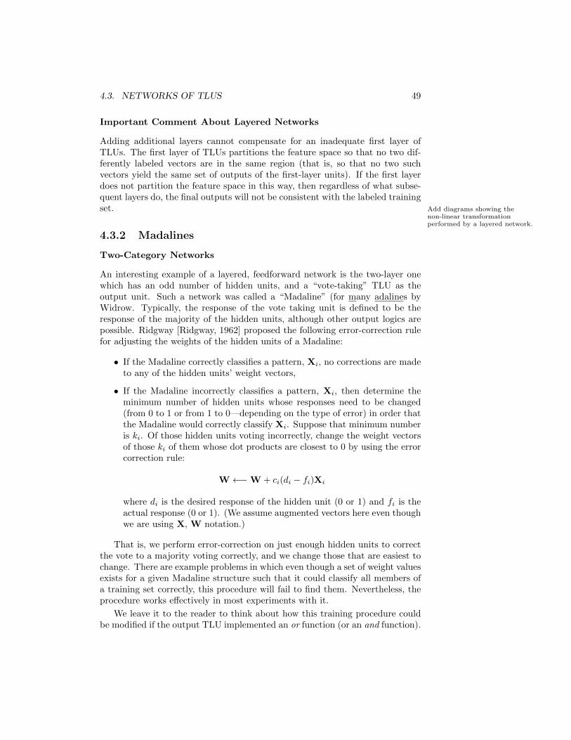
4.3. NETWORKS OF TLUS 49
Important Comment About Layered Networks
Adding additional layers cannot compensate for an inadequate first layer ofTLUs. The first layer of TLUs partitions the feature space so that no two dif-ferently labeled vectors are in the same region (that is, so that no two suchvectors yield the same set of outputs of the first-layer units). If the first layerdoes not partition the feature space in this way, then regardless of what subse-quent layers do, the final outputs will not be consistent with the labeled trainingset. Add diagrams showing the
non-linear transformationperformed by a layered network.
4.3.2 Madalines
Two-Category Networks
An interesting example of a layered, feedforward network is the two-layer onewhich has an odd number of hidden units, and a “vote-taking” TLU as theoutput unit. Such a network was called a “Madaline” (for many adalines byWidrow. Typically, the response of the vote taking unit is defined to be theresponse of the majority of the hidden units, although other output logics arepossible. Ridgway [Ridgway, 1962] proposed the following error-correction rulefor adjusting the weights of the hidden units of a Madaline:
• If the Madaline correctly classifies a pattern, Xi, no corrections are madeto any of the hidden units’ weight vectors,
• If the Madaline incorrectly classifies a pattern, Xi, then determine theminimum number of hidden units whose responses need to be changed(from 0 to 1 or from 1 to 0—depending on the type of error) in order thatthe Madaline would correctly classify Xi. Suppose that minimum numberis ki. Of those hidden units voting incorrectly, change the weight vectorsof those ki of them whose dot products are closest to 0 by using the errorcorrection rule:
W←−W + ci(di − fi)Xi
where di is the desired response of the hidden unit (0 or 1) and fi is theactual response (0 or 1). (We assume augmented vectors here even thoughwe are using X, W notation.)
That is, we perform error-correction on just enough hidden units to correctthe vote to a majority voting correctly, and we change those that are easiest tochange. There are example problems in which even though a set of weight valuesexists for a given Madaline structure such that it could classify all members ofa training set correctly, this procedure will fail to find them. Nevertheless, theprocedure works effectively in most experiments with it.
We leave it to the reader to think about how this training procedure couldbe modified if the output TLU implemented an or function (or an and function).
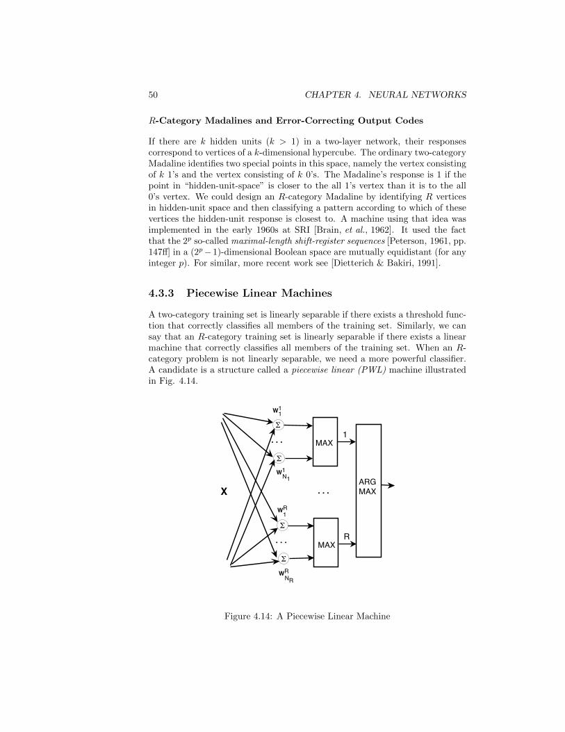
50 CHAPTER 4. NEURAL NETWORKS
R-Category Madalines and Error-Correcting Output Codes
If there are k hidden units (k > 1) in a two-layer network, their responsescorrespond to vertices of a k-dimensional hypercube. The ordinary two-categoryMadaline identifies two special points in this space, namely the vertex consistingof k 1’s and the vertex consisting of k 0’s. The Madaline’s response is 1 if thepoint in “hidden-unit-space” is closer to the all 1’s vertex than it is to the all0’s vertex. We could design an R-category Madaline by identifying R verticesin hidden-unit space and then classifying a pattern according to which of thesevertices the hidden-unit response is closest to. A machine using that idea wasimplemented in the early 1960s at SRI [Brain, et al., 1962]. It used the factthat the 2p so-called maximal-length shift-register sequences [Peterson, 1961, pp.147ff] in a (2p−1)-dimensional Boolean space are mutually equidistant (for anyinteger p). For similar, more recent work see [Dietterich & Bakiri, 1991].
4.3.3 Piecewise Linear Machines
A two-category training set is linearly separable if there exists a threshold func-tion that correctly classifies all members of the training set. Similarly, we cansay that an R-category training set is linearly separable if there exists a linearmachine that correctly classifies all members of the training set. When an R-category problem is not linearly separable, we need a more powerful classifier.A candidate is a structure called a piecewise linear (PWL) machine illustratedin Fig. 4.14.
X
W1
W1
. . . MAX
. . . MAX
. . .
WR
WR
ARGMAX
1
R
1
N1
1
NR
Figure 4.14: A Piecewise Linear Machine
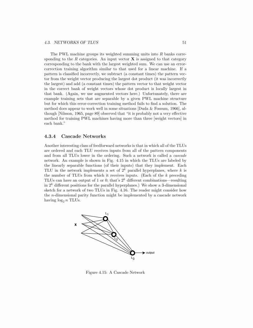
4.3. NETWORKS OF TLUS 51
The PWL machine groups its weighted summing units into R banks corre-sponding to the R categories. An input vector X is assigned to that categorycorresponding to the bank with the largest weighted sum. We can use an error-correction training algorithm similar to that used for a linear machine. If apattern is classified incorrectly, we subtract (a constant times) the pattern vec-tor from the weight vector producing the largest dot product (it was incorrectlythe largest) and add (a constant times) the pattern vector to that weight vectorin the correct bank of weight vectors whose dot product is locally largest inthat bank. (Again, we use augmented vectors here.) Unfortunately, there areexample training sets that are separable by a given PWL machine structurebut for which this error-correction training method fails to find a solution. Themethod does appear to work well in some situations [Duda & Fossum, 1966], al-though [Nilsson, 1965, page 89] observed that “it is probably not a very effectivemethod for training PWL machines having more than three [weight vectors] ineach bank.”
4.3.4 Cascade Networks
Another interesting class of feedforward networks is that in which all of the TLUsare ordered and each TLU receives inputs from all of the pattern componentsand from all TLUs lower in the ordering. Such a network is called a cascadenetwork. An example is shown in Fig. 4.15 in which the TLUs are labeled bythe linearly separable functions (of their inputs) that they implement. EachTLU in the network implements a set of 2k parallel hyperplanes, where k isthe number of TLUs from which it receives inputs. (Each of the k precedingTLUs can have an output of 1 or 0; that’s 2k different combinations—resultingin 2k different positions for the parallel hyperplanes.) We show a 3-dimensionalsketch for a network of two TLUs in Fig. 4.16. The reader might consider howthe n-dimensional parity function might be implemented by a cascade networkhaving log2 n TLUs.
x
L1
L2
outputL3
Figure 4.15: A Cascade Network
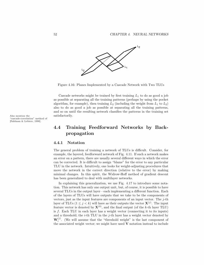
52 CHAPTER 4. NEURAL NETWORKS
L1
L2
L2
Figure 4.16: Planes Implemented by a Cascade Network with Two TLUs
Cascade networks might be trained by first training L1 to do as good a jobas possible at separating all the training patterns (perhaps by using the pocketalgorithm, for example), then training L2 (including the weight from L1 to L2)also to do as good a job as possible at separating all the training patterns,and so on until the resulting network classifies the patterns in the training setsatisfactorily.Also mention the
“cascade-correlation” method of[Fahlman & Lebiere, 1990].
4.4 Training Feedforward Networks by Back-propagation
4.4.1 Notation
The general problem of training a network of TLUs is difficult. Consider, forexample, the layered, feedforward network of Fig. 4.11. If such a network makesan error on a pattern, there are usually several different ways in which the errorcan be corrected. It is difficult to assign “blame” for the error to any particularTLU in the network. Intuitively, one looks for weight-adjusting procedures thatmove the network in the correct direction (relative to the error) by makingminimal changes. In this spirit, the Widrow-Hoff method of gradient descenthas been generalized to deal with multilayer networks.
In explaining this generalization, we use Fig. 4.17 to introduce some nota-tion. This network has only one output unit, but, of course, it is possible to haveseveral TLUs in the output layer—each implementing a different function. Eachof the layers of TLUs will have outputs that we take to be the components ofvectors, just as the input features are components of an input vector. The j-thlayer of TLUs (1 ≤ j < k) will have as their outputs the vector X(j). The inputfeature vector is denoted by X(0), and the final output (of the k-th layer TLU)is f . Each TLU in each layer has a weight vector (connecting it to its inputs)and a threshold; the i-th TLU in the j-th layer has a weight vector denoted by
W(j)i . (We will assume that the “threshold weight” is the last component of
the associated weight vector; we might have used V notation instead to include
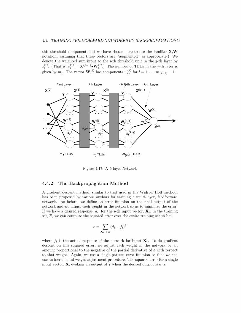
4.4. TRAINING FEEDFORWARDNETWORKS BY BACKPROPAGATION53
this threshold component, but we have chosen here to use the familiar X,Wnotation, assuming that these vectors are “augmented” as appropriate.) Wedenote the weighted sum input to the i-th threshold unit in the j-th layer by
s(j)i . (That is, s
(j)i = X(j−1)•W(j)
i .) The number of TLUs in the j-th layer is
given by mj . The vector W(j)i has components w
(j)l,i for l = 1, . . . ,m(j−1) + 1.
X(0)
. . .
. . .
. . .
. . .
Wi(1)
W(k)
X(1)
m1 TLUs
. . .Wi
(j)
. . .
X(j)
. . .Wi
(k-1)
X(k-1)
mj TLUs m(k-1) TLUs
wli(j)
wl(k)
First Layer j-th Layer (k-1)-th Layer k-th Layer
. . .
f
si(1) si(j) si(k-1)s(k)
Figure 4.17: A k-layer Network
4.4.2 The Backpropagation Method
A gradient descent method, similar to that used in the Widrow Hoff method,has been proposed by various authors for training a multi-layer, feedforwardnetwork. As before, we define an error function on the final output of thenetwork and we adjust each weight in the network so as to minimize the error.If we have a desired response, di, for the i-th input vector, Xi, in the trainingset, Ξ, we can compute the squared error over the entire training set to be:
ε =∑
Xi ε Ξ
(di − fi)2
where fi is the actual response of the network for input Xi. To do gradientdescent on this squared error, we adjust each weight in the network by anamount proportional to the negative of the partial derivative of ε with respectto that weight. Again, we use a single-pattern error function so that we canuse an incremental weight adjustment procedure. The squared error for a singleinput vector, X, evoking an output of f when the desired output is d is:
54 CHAPTER 4. NEURAL NETWORKS
ε = (d− f)2
It is convenient to take the partial derivatives of ε with respect to the variousweights in groups corresponding to the weight vectors. We define a partial
derivative of a quantity φ, say, with respect to a weight vector, W(j)i , thus:
∂φ
∂W(j)i
def=
[∂φ
∂w(j)1i
, . . . ,∂φ
∂w(j)li
, . . . ,∂φ
∂w(j)mj−1+1,i
]
where w(j)li is the l-th component of W
(j)i . This vector partial derivative of φ is
called the gradient of φ with respect to W and is sometimes denoted by ∇Wφ.
Since ε’s dependence on W(j)i is entirely through s
(j)i , we can use the chain
rule to write:
∂ε
∂W(j)i
=∂ε
∂s(j)i
∂s(j)i
∂W(j)i
Because s(j)i = X(j−1)•W(j)
i ,∂s
(j)i
∂W(j)i
= X(j−1). Substituting yields:
∂ε
∂W(j)i
=∂ε
∂s(j)i
X(j−1)
Note that ∂ε
∂s(j)i
= −2(d− f) ∂f
∂s(j)i
. Thus,
∂ε
∂W(j)i
= −2(d− f)∂f
∂s(j)i
X(j−1)
The quantity (d−f) ∂f
∂s(j)i
plays an important role in our calculations; we shall
denote it by δ(j)i . Each of the δ
(j)i ’s tells us how sensitive the squared error of
the network output is to changes in the input to each threshold function. Sincewe will be changing weight vectors in directions along their negative gradient,our fundamental rule for weight changes throughout the network will be:
W(j)i ←W
(j)i + c
(j)i δ
(j)i X(j−1)
where c(j)i is the learning rate constant for this weight vector. (Usually, the
learning rate constants for all weight vectors in the network are the same.) Wesee that this rule is quite similar to that used in the error correction procedure
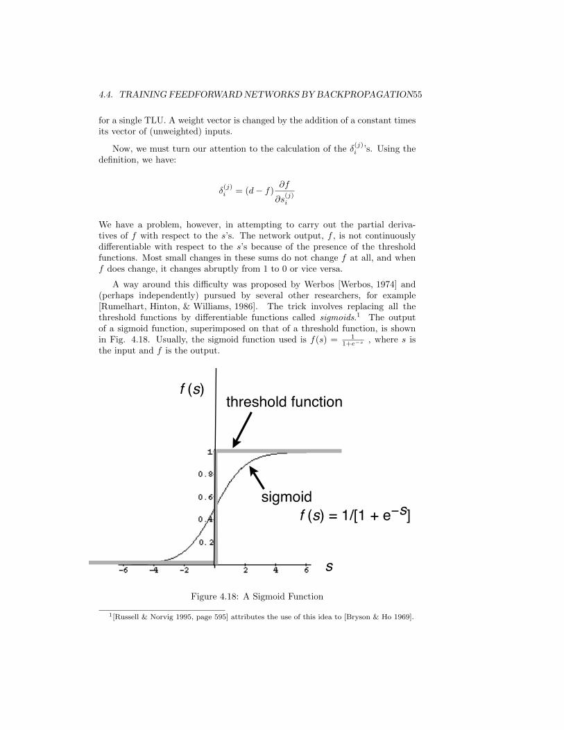
4.4. TRAINING FEEDFORWARDNETWORKS BY BACKPROPAGATION55
for a single TLU. A weight vector is changed by the addition of a constant timesits vector of (unweighted) inputs.
Now, we must turn our attention to the calculation of the δ(j)i ’s. Using the
definition, we have:
δ(j)i = (d− f)
∂f
∂s(j)i
We have a problem, however, in attempting to carry out the partial deriva-tives of f with respect to the s’s. The network output, f , is not continuouslydifferentiable with respect to the s’s because of the presence of the thresholdfunctions. Most small changes in these sums do not change f at all, and whenf does change, it changes abruptly from 1 to 0 or vice versa.
A way around this difficulty was proposed by Werbos [Werbos, 1974] and(perhaps independently) pursued by several other researchers, for example[Rumelhart, Hinton, & Williams, 1986]. The trick involves replacing all thethreshold functions by differentiable functions called sigmoids.1 The outputof a sigmoid function, superimposed on that of a threshold function, is shownin Fig. 4.18. Usually, the sigmoid function used is f(s) = 1
1+e−s , where s isthe input and f is the output.
sigmoid
threshold functionf (s)
s
f (s) = 1/[1 + e s]
Figure 4.18: A Sigmoid Function
1[Russell & Norvig 1995, page 595] attributes the use of this idea to [Bryson & Ho 1969].
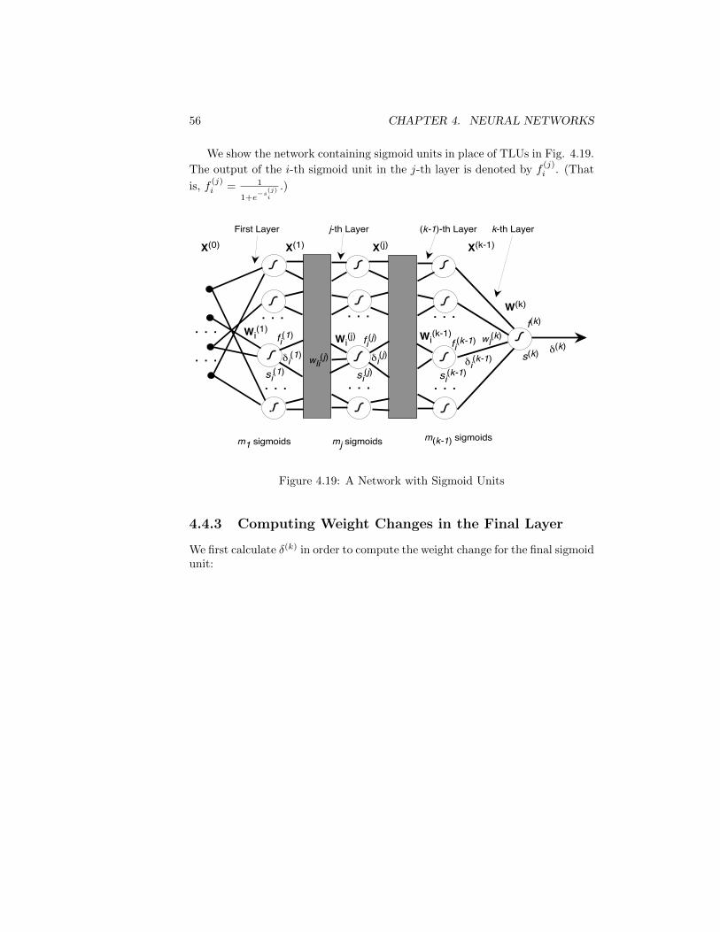
56 CHAPTER 4. NEURAL NETWORKS
We show the network containing sigmoid units in place of TLUs in Fig. 4.19.
The output of the i-th sigmoid unit in the j-th layer is denoted by f(j)i . (That
is, f(j)i = 1
1+e−s(j)i
.)
X(0)
. . .
. . .
. . .
. . .
Wi(1)
si(1)
W(k)
X(1)
fi(1)
m1 sigmoids
. . .Wi
(j) fi(j)
si(j) . . .
X(j)
. . .Wi
(k-1)fi(k-1)
si(k-1)
f(k)
s(k)
X(k-1)
mj sigmoids m(k-1) sigmoids
wli(j)
wl(k)
i(j)
i(1)
i(k-1)
(k)
First Layer j-th Layer (k-1)-th Layer k-th Layer
. . .
Figure 4.19: A Network with Sigmoid Units
4.4.3 Computing Weight Changes in the Final Layer
We first calculate δ(k) in order to compute the weight change for the final sigmoidunit:
4.4. TRAINING FEEDFORWARDNETWORKS BY BACKPROPAGATION57
δ(k) = (d− f (k))∂f (k)
∂s(k)
Given the sigmoid function that we are using, namely f(s) = 11+e−s , we have
that ∂f∂s = f(1− f). Substituting gives us:
δ(k) = (d− f (k))f (k)(1− f (k))
Rewriting our general rule for weight vector changes, the weight vector inthe final layer is changed according to the rule:
W(k) ←W(k) + c(k)δ(k)X(k−1)
where δ(k) = (d− f (k))f (k)(1− f (k))
It is interesting to compare backpropagation to the error-correction rule andto the Widrow-Hoff rule. The backpropagation weight adjustment for the singleelement in the final layer can be written as:
W←−W + c(d− f)f(1− f)X
Written in the same format, the error-correction rule is:
W←−W + c(d− f)X
and the Widrow-Hoff rule is:
W←−W + c(d− f)X
The only difference (except for the fact that f is not thresholded in Widrow-Hoff) is the f(1 − f) term due to the presence of the sigmoid function. Withthe sigmoid function, f(1 − f) can vary in value from 0 to 1. When f is 0,f(1 − f) is also 0; when f is 1, f(1 − f) is 0; f(1 − f) obtains its maximumvalue of 1/4 when f is 1/2 (that is, when the input to the sigmoid is 0). Thesigmoid function can be thought of as implementing a “fuzzy” hyperplane. Fora pattern far away from this fuzzy hyperplane, f(1 − f) has value close to 0,and the backpropagation rule makes little or no change to the weight valuesregardless of the desired output. (Small changes in the weights will have littleeffect on the output for inputs far from the hyperplane.) Weight changes areonly made within the region of “fuzz” surrounding the hyperplane, and thesechanges are in the direction of correcting the error, just as in the error-correctionand Widrow-Hoff rules.
58 CHAPTER 4. NEURAL NETWORKS
4.4.4 Computing Changes to the Weights in IntermediateLayers
Using our expression for the δ’s, we can similarly compute how to change eachof the weight vectors in the network. Recall:
δ(j)i = (d− f)
∂f
∂s(j)i
Again we use a chain rule. The final output, f , depends on s(j)i through
each of the summed inputs to the sigmoids in the (j + 1)-th layer. So:
δ(j)i = (d− f)
∂f
∂s(j)i
= (d− f)
[∂f
∂s(j+1)1
∂s(j+1)1
∂s(j)i
+ · · ·+ ∂f
∂s(j+1)l
∂s(j+1)l
∂s(j)i
+ · · ·+ ∂f
∂s(j+1)mj+1
∂s(j+1)mj+1
∂s(j)i
]
=
mj+1∑l=1
(d− f)∂f
∂s(j+1)l
∂s(j+1)l
∂s(j)i
=
mj+1∑l=1
δ(j+1)l
∂s(j+1)l
∂s(j)i
It remains to compute the∂s
(j+1)
l
∂s(j)i
’s. To do that we first write:
s(j+1)l = X(j)•W(j+1)
l
=
mj+1∑ν=1
f (j)ν w
(j+1)νl
And then, since the weights do not depend on the s’s:
∂s(j+1)l
∂s(j)i
=∂[∑mj+1
ν=1 f(j)ν w
(j+1)νl
]∂s
(j)i
=
mj+1∑ν=1
w(j+1)νl
∂f(j)ν
∂s(j)i
Now, we note that∂f(j)ν
∂s(j)i
= 0 unless ν = i, in which case∂f(j)ν
∂s(j)ν
= f(j)ν (1 − f (j)
ν ).
Therefore:
∂s(j+1)l
∂s(j)i
= w(j+1)il f
(j)i (1− f (j)
i )
4.4. TRAINING FEEDFORWARDNETWORKS BY BACKPROPAGATION59
We use this result in our expression for δ(j)i to give:
δ(j)i = f
(j)i (1− f (j)
i )
mj+1∑l=1
δ(j+1)l w
(j+1)il
The above equation is recursive in the δ’s. (It is interesting to note thatthis expression is independent of the error function; the error function explicitly
affects only the computation of δ(k).) Having computed the δ(j+1)i ’s for layer
j + 1, we can use this equation to compute the δ(j)i ’s. The base case is δ(k),
which we have already computed:
δ(k) = (d− f (k))f (k)(1− f (k))
We use this expression for the δ’s in our generic weight changing rule, namely:
W(j)i ←W
(j)i + c
(j)i δ
(j)i X(j−1)
Although this rule appears complex, it has an intuitively reasonable explanation.The quantity δ(k) = (d− f)f(1− f) controls the overall amount and sign of allweight adjustments in the network. (Adjustments diminish as the final output,f , approaches either 0 or 1, because they have vanishing effect on f then.) Asthe recursion equation for the δ’s shows, the adjustments for the weights goingin to a sigmoid unit in the j-th layer are proportional to the effect that suchadjustments have on that sigmoid unit’s output (its f (j)(1−f (j)) factor). Theyare also proportional to a kind of “average” effect that any change in the outputof that sigmoid unit will have on the final output. This average effect dependson the weights going out of the sigmoid unit in the j-th layer (small weightsproduce little downstream effect) and the effects that changes in the outputs of(j + 1)-th layer sigmoid units will have on the final output (as measured by theδ(j+1)’s). These calculations can be simply implemented by “backpropagating”the δ’s through the weights in reverse direction (thus, the name backprop forthis algorithm).
4.4.5 Variations on Backprop
[To be written: problem of local minima, simulated annealing, momemtum(Plaut, et al., 1986, see [Hertz, Krogh, & Palmer, 1991]), quickprop, regulariza-tion methods]
Simulated Annealing
To apply simulated annealing, the value of the learning rate constant is graduallydecreased with time. If we fall early into an error-function valley that is notvery deep (a local minimum), it typically will neither be very broad, and soon
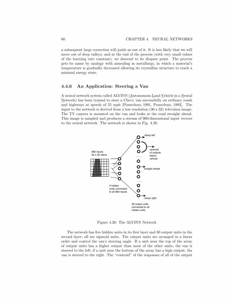
60 CHAPTER 4. NEURAL NETWORKS
a subsequent large correction will jostle us out of it. It is less likely that we willmove out of deep valleys, and at the end of the process (with very small valuesof the learning rate constant), we descend to its deepest point. The processgets its name by analogy with annealing in metallurgy, in which a material’stemperature is gradually decreased allowing its crystalline structure to reach aminimal energy state.
4.4.6 An Application: Steering a Van
A neural network system called ALVINN (Autonomous Land Vehicle in a NeuralNetwork) has been trained to steer a Chevy van successfully on ordinary roadsand highways at speeds of 55 mph [Pomerleau, 1991, Pomerleau, 1993]. Theinput to the network is derived from a low-resolution (30 x 32) television image.The TV camera is mounted on the van and looks at the road straight ahead.This image is sampled and produces a stream of 960-dimensional input vectorsto the neural network. The network is shown in Fig. 4.20.
960 inputs30 x 32 retina
. . .5 hiddenunits connectedto all 960 inputs
30 output unitsconnected to allhidden units
. . .
sharp left
sharp right
straight ahead
centroidof outputssteersvehicle
Figure 4.20: The ALVINN Network
The network has five hidden units in its first layer and 30 output units in thesecond layer; all are sigmoid units. The output units are arranged in a linearorder and control the van’s steering angle. If a unit near the top of the arrayof output units has a higher output than most of the other units, the van issteered to the left; if a unit near the bottom of the array has a high output, thevan is steered to the right. The “centroid” of the responses of all of the output
4.5. SYNERGIES BETWEENNEURAL NETWORKANDKNOWLEDGE-BASEDMETHODS61
units is computed, and the van’s steering angle is set at a corresponding valuebetween hard left and hard right.
The system is trained by a modified on-line training regime. A driver drivesthe van, and his actual steering angles are taken as the correct labels for thecorresponding inputs. The network is trained incrementally by backprop toproduce the driver-specified steering angles in response to each visual patternas it occurs in real time while driving.
This simple procedure has been augmented to avoid two potential problems.First, since the driver is usually driving well, the network would never get anyexperience with far-from-center vehicle positions and/or incorrect vehicle orien-tations. Also, on long, straight stretches of road, the network would be trainedfor a long time only to produce straight-ahead steering angles; this trainingwould swamp out earlier training to follow a curved road. We wouldn’t wantto try to avoid these problems by instructing the driver to drive erraticallyoccasionally, because the system would learn to mimic this erratic behavior.
Instead, each original image is shifted and rotated in software to create 14additional images in which the vehicle appears to be situated differently relativeto the road. Using a model that tells the system what steering angle ought tobe used for each of these shifted images, given the driver-specified steering anglefor the original image, the system constructs an additional 14 labeled trainingpatterns to add to those encountered during ordinary driver training.
4.5 Synergies Between Neural Network andKnowledge-Based Methods
To be written; discussrule-generating procedures (such as[Towell & Shavlik, 1992]) and howexpert-provided rules can aidneural net training and vice-versa[Towell, Shavlik, & Noordweier, 1990].
4.6 Bibliographical and Historical Remarks
To be added.

62 CHAPTER 4. NEURAL NETWORKS
Chapter 5
Statistical Learning
5.1 Using Statistical Decision Theory
5.1.1 Background and General Method
Suppose the pattern vector, X, is a random variable whose probability distri-bution for category 1 is different than it is for category 2. (The treatment givenhere can easily be generalized to R-category problems.) Specifically, suppose wehave the two probability distributions (perhaps probability density functions),p(X | 1) and p(X | 2). Given a pattern, X, we want to use statistical tech-niques to determine its category—that is, to determine from which distributionit was drawn. These techniques are based on the idea of minimizing the ex-pected value of a quantity similar to the error function we used in deriving theweight-changing rules for backprop.
In developing a decision method, it is necessary to know the relative serious-ness of the two kinds of mistakes that might be made. (We might decide that apattern really in category 1 is in category 2, and vice versa.) We describe thisinformation by a loss function, λ(i | j), for i, j = 1, 2. λ(i | j) represents the lossincurred when we decide a pattern is in category i when really it is in categoryj. We assume here that λ(1 | 1) and λ(2 | 2) are both 0. For any given pattern,X, we want to decide its category in such a way that minimizes the expectedvalue of this loss.
Given a pattern, X, if we decide category i, the expected value of the losswill be:
LX(i) = λ(i | 1)p(1 | X) + λ(i | 2)p(2 | X)
where p(j | X) is the probability that given a pattern X, its category is j. Ourdecision rule will be to decide that X belongs to category 1 if LX(1) ≤ LX(2),and to decide on category 2 otherwise.
63
64 CHAPTER 5. STATISTICAL LEARNING
We can use Bayes’ Rule to get expressions for p(j | X) in terms of p(X | j),which we assume to be known (or estimatible):
p(j | X) =p(X | j)p(j)
p(X)
where p(j) is the (a priori) probability of category j (one category may be muchmore probable than the other); and p(X) is the (a priori) probability of patternX being the pattern we are asked to classify. Performing the substitutions givenby Bayes’ Rule, our decision rule becomes:
Decide category 1 iff:
λ(1 | 1)p(X | 1)p(1)
p(X)+ λ(1 | 2)
p(X | 2)p(2)
p(X)
≤ λ(2 | 1)p(X | 1)p(1)
p(X)+ λ(2 | 2)
p(X | 2)p(2)
p(X)
Using the fact that λ(i | i) = 0, and noticing that p(X) is common to bothexpressions, we obtain,
Decide category 1 iff:
λ(1 | 2)p(X | 2)p(2) ≤ λ(2 | 1)p(X | 1)p(1)
If λ(1 | 2) = λ(2 | 1) and if p(1) = p(2), then the decision becomes particu-larly simple:
Decide category 1 iff:
p(X | 2) ≤ p(X | 1)
Since p(X | j) is called the likelihood of j with respect to X, this simple decisionrule implements what is called a maximum-likelihood decision. More generally,if we define k(i | j) as λ(i | j)p(j), then our decision rule is simply,
Decide category1 iff:
k(1 | 2)p(X | 2) ≤ k(2 | 1)p(X | 1)
In any case, we need to compare the (perhaps weighted) quantities p(X | i) fori = 1 and 2. The exact decision rule depends on the the probability distributionsassumed. We will treat two interesting distributions.
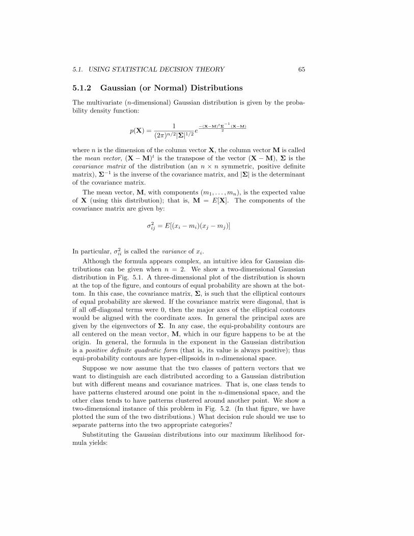
5.1. USING STATISTICAL DECISION THEORY 65
5.1.2 Gaussian (or Normal) Distributions
The multivariate (n-dimensional) Gaussian distribution is given by the proba-bility density function:
p(X) =1
(2π)n/2|Σ|1/2e−(X−M)tΣ
−1(X−M)
2
where n is the dimension of the column vector X, the column vector M is calledthe mean vector, (X −M)t is the transpose of the vector (X −M), Σ is thecovariance matrix of the distribution (an n × n symmetric, positive definitematrix), Σ−1 is the inverse of the covariance matrix, and |Σ| is the determinantof the covariance matrix.
The mean vector, M, with components (m1, . . . ,mn), is the expected valueof X (using this distribution); that is, M = E[X]. The components of thecovariance matrix are given by:
σ2ij = E[(xi −mi)(xj −mj)]
In particular, σ2ii is called the variance of xi.
Although the formula appears complex, an intuitive idea for Gaussian dis-tributions can be given when n = 2. We show a two-dimensional Gaussiandistribution in Fig. 5.1. A three-dimensional plot of the distribution is shownat the top of the figure, and contours of equal probability are shown at the bot-tom. In this case, the covariance matrix, Σ, is such that the elliptical contoursof equal probability are skewed. If the covariance matrix were diagonal, that isif all off-diagonal terms were 0, then the major axes of the elliptical contourswould be aligned with the coordinate axes. In general the principal axes aregiven by the eigenvectors of Σ. In any case, the equi-probability contours areall centered on the mean vector, M, which in our figure happens to be at theorigin. In general, the formula in the exponent in the Gaussian distributionis a positive definite quadratic form (that is, its value is always positive); thusequi-probability contours are hyper-ellipsoids in n-dimensional space.
Suppose we now assume that the two classes of pattern vectors that wewant to distinguish are each distributed according to a Gaussian distributionbut with different means and covariance matrices. That is, one class tends tohave patterns clustered around one point in the n-dimensional space, and theother class tends to have patterns clustered around another point. We show atwo-dimensional instance of this problem in Fig. 5.2. (In that figure, we haveplotted the sum of the two distributions.) What decision rule should we use toseparate patterns into the two appropriate categories?
Substituting the Gaussian distributions into our maximum likelihood for-mula yields:
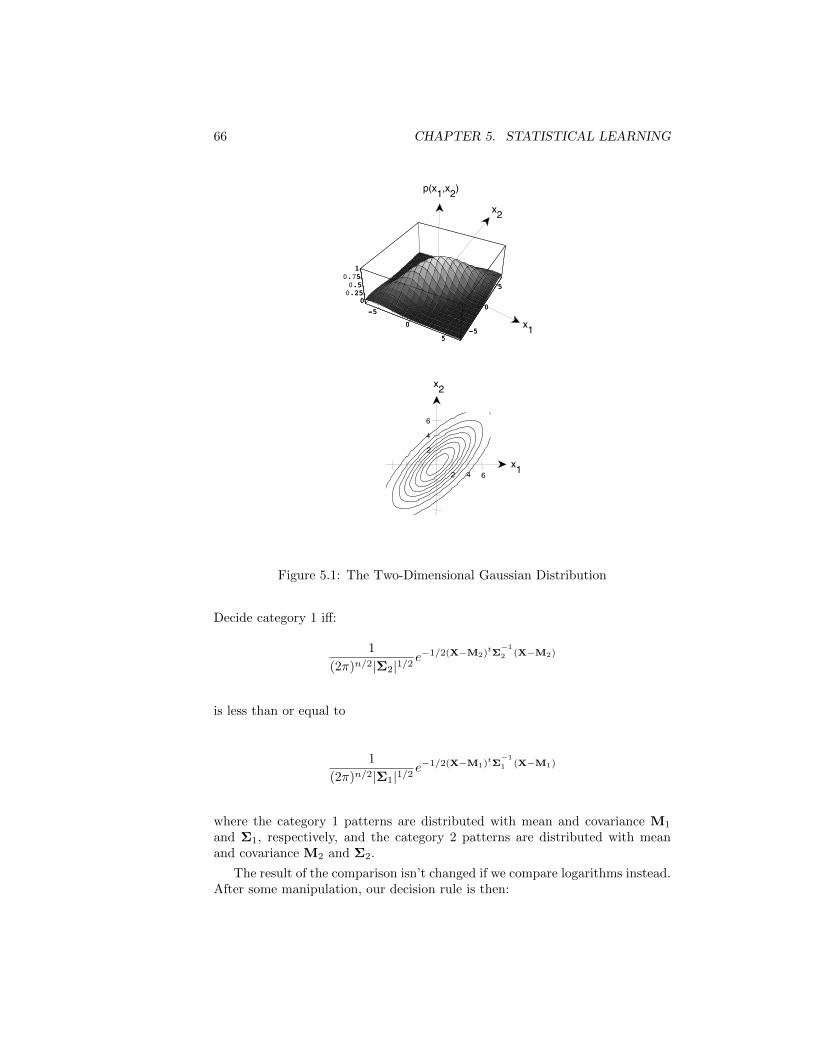
66 CHAPTER 5. STATISTICAL LEARNING
-5
0
5-5
0
5
00.250.5
0.751
-5
0
5-5
0
5
025.5751
-6 -4 -2 0 2 4 6
-6
-4
-2
0
2
4
6
x1
x2
p(x1,x2)
2
4
6
2 4 6x1
x2
Figure 5.1: The Two-Dimensional Gaussian Distribution
Decide category 1 iff:
1
(2π)n/2|Σ2|1/2e−1/2(X−M2)tΣ
−1
2 (X−M2)
is less than or equal to
1
(2π)n/2|Σ1|1/2e−1/2(X−M1)tΣ
−1
1 (X−M1)
where the category 1 patterns are distributed with mean and covariance M1
and Σ1, respectively, and the category 2 patterns are distributed with meanand covariance M2 and Σ2.
The result of the comparison isn’t changed if we compare logarithms instead.After some manipulation, our decision rule is then:
5.1. USING STATISTICAL DECISION THEORY 67
-50
5
10
-5
0
5
10
00.250.5
0.751
-50
5
10
-5
0
5
10
025.5751
x1
x2
p(x1,x2)
-5 -2.5 0 2.5 5 7.5 10
-5
-2.5
0
2.5
5
7.5
10
Figure 5.2: The Sum of Two Gaussian Distributions
Decide category 1 iff:
(X−M1)tΣ−11 (X−M1) < (X−M2)tΣ−1
2 (X−M2) +B
where B, a constant bias term, incorporates the logarithms of the fractionspreceding the exponential, etc.
When the quadratic forms are multiplied out and represented in terms ofthe components xi, the decision rule involves a quadric surface (a hyperquadric)in n-dimensional space. The exact shape and position of this hyperquadric isdetermined by the means and the covariance matrices. The surface separatesthe space into two parts, one of which contains points that will be assigned tocategory 1 and the other contains points that will be assigned to category 2.
It is interesting to look at a special case of this surface. If the covariancematrices for each category are identical and diagonal, with all σii equal to eachother, then the contours of equal probability for each of the two distributions
68 CHAPTER 5. STATISTICAL LEARNING
are hyperspherical. The quadric forms then become (1/|Σ|)(X−Mi)t(X−Mi),
and the decision rule is:
Decide category 1 iff:
(X−M1)t(X−M1) < (X−M2)t(X−M2)
Multiplying out yields:
X•X− 2X•M1 + M1•M1 < X•X− 2X•M2 + M2•M2
or finally,
Decide category 1 iff:
X•M1 ≥ X•M2 + Constant
or
X•(M1 −M2) ≥ Constant
where the constant depends on the lengths of the mean vectors.
We see that the optimal decision surface in this special case is a hyperplane.In fact, the hyperplane is perpendicular to the line joining the two means. Theweights in a TLU implementation are equal to the difference in the mean vectors.
If the parameters (Mi,Σi) of the probability distributions of the categoriesare not known, there are various techniques for estimating them, and then usingthose estimates in the decision rule. For example, if there are sufficient trainingpatterns, one can use sample means and sample covariance matrices. (Caution:the sample covariance matrix will be singular if the training patterns happen tolie on a subspace of the whole n-dimensional space—as they certainly will, forexample, if the number of training patterns is less than n.)
5.1.3 Conditionally Independent Binary Components
Suppose the vector X is a random variable having binary (0,1) components.We continue to denote the two probability distributions by p(X | 1) and p(X |2). Further suppose that the components of these vectors are conditionallyindependent given the category. By conditional independence in this case, wemean that the formulas for the distribution can be expanded as follows:
5.1. USING STATISTICAL DECISION THEORY 69
p(X | i) = p(x1 | i)p(x2 | i) · · · p(xn | i)
for i = 1, 2
Recall the minimum-average-loss decision rule,
Decide category 1 iff:
λ(1 | 2)p(X | 2)p(2) ≤ λ(2 | 1)p(X | 1)p(1)
Assuming conditional independence of the components and that λ(1 | 2) = λ(2 |1), we obtain,
Decide category 1 iff:
p(1)p(x1 | 1)p(x2 | 1) · · · p(xn | 1) ≥ p(x1 | 2)p(x2 | 2) · · · p(xn | 2)p(2)
or iff:
p(x1 | 1)p(x2 | 1) . . . p(xn | 1)
p(x1 | 2)p(x2 | 2) . . . p(xn | 2)≥ p(2)
p(1)
or iff:
logp(x1 | 1)
p(x1 | 2)+ log
p(x2 | 1)
p(x2 | 2)+ · · ·+ log
p(xn | 1)
p(xn | 2)+ log
p(1)
p(2)≥ 0
Let us define values of the components of the distribution for specific values oftheir arguments, xi :
p(xi = 1 | 1) = pi
p(xi = 0 | 1) = 1− pip(xi = 1 | 2) = qi
p(xi = 0 | 2) = 1− qiNow, we note that since xi can only assume the values of 1 or 0:
logp(xi | 1)
p(xi | 2)= xi log
piqi
+ (1− xi) log(1− pi)(1− qi)
70 CHAPTER 5. STATISTICAL LEARNING
= xi logpi(1− qi)qi(1− pi)
+ log(1− pi)(1− qi)
Substituting these expressions into our decision rule yields:
Decide category 1 iff:
n∑i=1
xi logpi(1− qi)qi(1− pi)
+
n∑i=1
log(1− pi)(1− qi)
+ logp(1)
p(2)≥ 0
We see that we can achieve this decision with a TLU with weight values asfollows:
wi = logpi(1− qi)qi(1− pi)
for i = 1, . . . , n, and
wn+1 = logp(1)
1− p(1)+
n∑i=1
log(1− pi)(1− qi)
If we do not know the pi, qi and p(1), we can use a sample of labeled trainingpatterns to estimate these parameters.
5.2 Learning Belief NetworksTo be added.
5.3 Nearest-Neighbor Methods
Another class of methods can be related to the statistical ones. These are callednearest-neighbor methods or, sometimes, memory-based methods. (A collectionof papers on this subject is in [Dasarathy, 1991].) Given a training set Ξ of mlabeled patterns, a nearest-neighbor procedure decides that some new pattern,X, belongs to the same category as do its closest neighbors in Ξ. More precisely,a k-nearest-neighbor method assigns a new pattern, X, to that category to whichthe plurality of its k closest neighbors belong. Using relatively large values ofk decreases the chance that the decision will be unduly influenced by a noisytraining pattern close to X. But large values of k also reduce the acuity of themethod. The k-nearest-neighbor method can be thought of as estimating thevalues of the probabilities of the classes given X. Of course the denser are thepoints around X, and the larger the value of k, the better the estimate.
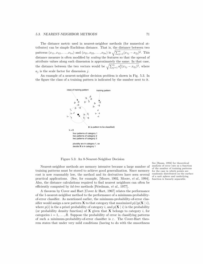
5.3. NEAREST-NEIGHBOR METHODS 71
The distance metric used in nearest-neighbor methods (for numerical at-tributes) can be simple Euclidean distance. That is, the distance between two
patterns (x11, x12, . . . , x1n) and (x21, x22, . . . , x2n) is√∑n
j=1(x1j − x2j)2. This
distance measure is often modified by scaling the features so that the spread ofattribute values along each dimension is approximately the same. In that case,
the distance between the two vectors would be√∑n
j=1 a2j (x1j − x2j)2, where
aj is the scale factor for dimension j.
An example of a nearest-neighbor decision problem is shown in Fig. 5.3. Inthe figure the class of a training pattern is indicated by the number next to it.
k = 8X (a pattern to be classified)
1
1
1 11
111
2
1
2
222
22 2
2
33
3
3
3
33
33
training patternclass of training pattern
four patterns of category 1two patterns of category 2two patterns of category 3
plurality are in category 1, sodecide X is in category 1
Figure 5.3: An 8-Nearest-Neighbor DecisionSee [Baum, 1994] for theoreticalanalysis of error rate as a functionof the number of training patternsfor the case in which points arerandomly distributed on the surfaceof a unit sphere and underlyingfunction is linearly separable.
Nearest-neighbor methods are memory intensive because a large number oftraining patterns must be stored to achieve good generalization. Since memorycost is now reasonably low, the method and its derivatives have seen severalpractical applications. (See, for example, [Moore, 1992, Moore, et al., 1994].Also, the distance calculations required to find nearest neighbors can often beefficiently computed by kd-tree methods [Friedman, et al., 1977].
A theorem by Cover and Hart [Cover & Hart, 1967] relates the performanceof the 1-nearest-neighbor method to the performance of a minimum-probability-of-error classifier. As mentioned earlier, the minimum-probability-of-error clas-sifier would assign a new pattern X to that category that maximized p(i)p(X | i),where p(i) is the a priori probability of category i, and p(X | i) is the probability(or probability density function) of X given that X belongs to category i, forcategories i = 1, . . . , R. Suppose the probability of error in classifying patternsof such a minimum-probability-of-error classifier is ε. The Cover-Hart theo-rem states that under very mild conditions (having to do with the smoothness
72 CHAPTER 5. STATISTICAL LEARNING
of probability density functions) the probability of error, εnn, of a 1-nearest-neighbor classifier is bounded by:
ε ≤ εnn ≤ ε(
2− ε R
R− 1
)≤ 2ε
where R is the number of categories.Also see [Aha, 1991].
5.4 Bibliographical and Historical RemarksTo be added.
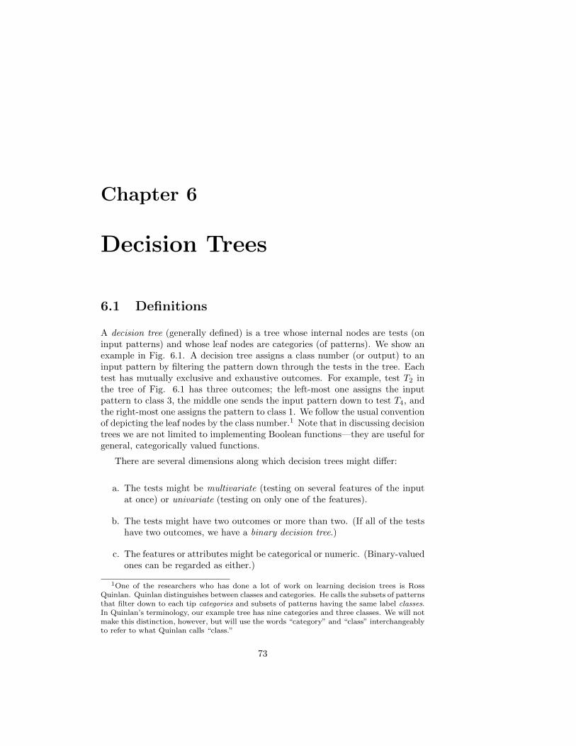
Chapter 6
Decision Trees
6.1 Definitions
A decision tree (generally defined) is a tree whose internal nodes are tests (oninput patterns) and whose leaf nodes are categories (of patterns). We show anexample in Fig. 6.1. A decision tree assigns a class number (or output) to aninput pattern by filtering the pattern down through the tests in the tree. Eachtest has mutually exclusive and exhaustive outcomes. For example, test T2 inthe tree of Fig. 6.1 has three outcomes; the left-most one assigns the inputpattern to class 3, the middle one sends the input pattern down to test T4, andthe right-most one assigns the pattern to class 1. We follow the usual conventionof depicting the leaf nodes by the class number.1 Note that in discussing decisiontrees we are not limited to implementing Boolean functions—they are useful forgeneral, categorically valued functions.
There are several dimensions along which decision trees might differ:
a. The tests might be multivariate (testing on several features of the inputat once) or univariate (testing on only one of the features).
b. The tests might have two outcomes or more than two. (If all of the testshave two outcomes, we have a binary decision tree.)
c. The features or attributes might be categorical or numeric. (Binary-valuedones can be regarded as either.)
1One of the researchers who has done a lot of work on learning decision trees is RossQuinlan. Quinlan distinguishes between classes and categories. He calls the subsets of patternsthat filter down to each tip categories and subsets of patterns having the same label classes.In Quinlan’s terminology, our example tree has nine categories and three classes. We will notmake this distinction, however, but will use the words “category” and “class” interchangeablyto refer to what Quinlan calls “class.”
73
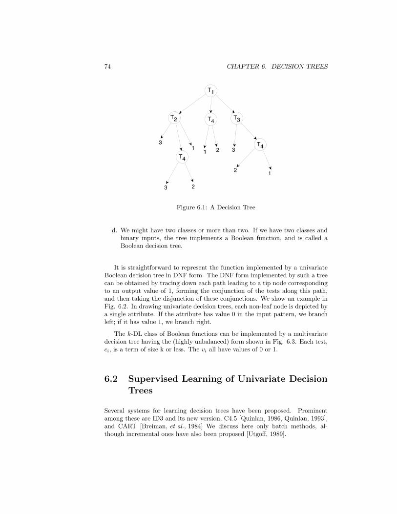
74 CHAPTER 6. DECISION TREES
T1
T2 T3
T4
T4
T4
31
3 2
1 2 3
2 1
Figure 6.1: A Decision Tree
d. We might have two classes or more than two. If we have two classes andbinary inputs, the tree implements a Boolean function, and is called aBoolean decision tree.
It is straightforward to represent the function implemented by a univariateBoolean decision tree in DNF form. The DNF form implemented by such a treecan be obtained by tracing down each path leading to a tip node correspondingto an output value of 1, forming the conjunction of the tests along this path,and then taking the disjunction of these conjunctions. We show an example inFig. 6.2. In drawing univariate decision trees, each non-leaf node is depicted bya single attribute. If the attribute has value 0 in the input pattern, we branchleft; if it has value 1, we branch right.
The k-DL class of Boolean functions can be implemented by a multivariatedecision tree having the (highly unbalanced) form shown in Fig. 6.3. Each test,ci, is a term of size k or less. The vi all have values of 0 or 1.
6.2 Supervised Learning of Univariate DecisionTrees
Several systems for learning decision trees have been proposed. Prominentamong these are ID3 and its new version, C4.5 [Quinlan, 1986, Quinlan, 1993],and CART [Breiman, et al., 1984] We discuss here only batch methods, al-though incremental ones have also been proposed [Utgoff, 1989].
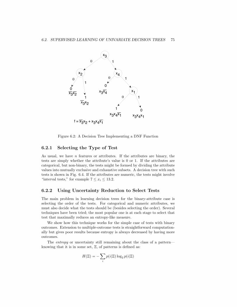
6.2. SUPERVISED LEARNING OF UNIVARIATE DECISION TREES 75
x3
x2 x4
x1
10
1
1
0 0
0
1
x3x2
x3x2
x3x4
x3x4x1 x3x4x1f = x3x2 + x3x4x1
1
00
1 0
Figure 6.2: A Decision Tree Implementing a DNF Function
6.2.1 Selecting the Type of Test
As usual, we have n features or attributes. If the attributes are binary, thetests are simply whether the attribute’s value is 0 or 1. If the attributes arecategorical, but non-binary, the tests might be formed by dividing the attributevalues into mutually exclusive and exhaustive subsets. A decision tree with suchtests is shown in Fig. 6.4. If the attributes are numeric, the tests might involve“interval tests,” for example 7 ≤ xi ≤ 13.2.
6.2.2 Using Uncertainty Reduction to Select Tests
The main problem in learning decision trees for the binary-attribute case isselecting the order of the tests. For categorical and numeric attributes, wemust also decide what the tests should be (besides selecting the order). Severaltechniques have been tried; the most popular one is at each stage to select thattest that maximally reduces an entropy-like measure.
We show how this technique works for the simple case of tests with binaryoutcomes. Extension to multiple-outcome tests is straightforward computation-ally but gives poor results because entropy is always decreased by having moreoutcomes.
The entropy or uncertainty still remaining about the class of a pattern—knowing that it is in some set, Ξ, of patterns is defined as:
H(Ξ) = −∑i
p(i|Ξ) log2 p(i|Ξ)
76 CHAPTER 6. DECISION TREES
cq
cq-1
ci
1
vn
vn-1
vi
v1
Figure 6.3: A Decision Tree Implementing a Decision List
where p(i|Ξ) is the probability that a pattern drawn at random from Ξ belongsto class i, and the summation is over all of the classes. We want to select tests ateach node such that as we travel down the decision tree, the uncertainty aboutthe class of a pattern becomes less and less.
Since we do not in general have the probabilities p(i|Ξ), we estimate them bysample statistics. Although these estimates might be errorful, they are never-theless useful in estimating uncertainties. Let p(i|Ξ) be the number of patternsin Ξ belonging to class i divided by the total number of patterns in Ξ. Then anestimate of the uncertainty is:
H(Ξ) = −∑i
p(i|Ξ) log2 p(i|Ξ)
For simplicity, from now on we’ll drop the “hats” and use sample statistics asif they were real probabilities.
If we perform a test, T , having k possible outcomes on the patterns in Ξ, wewill create k subsets, Ξ1,Ξ2, . . . ,Ξk. Suppose that ni of the patterns in Ξ are inΞi for i = 1, ..., k. (Some ni may be 0.) If we knew that T applied to a patternin Ξ resulted in the j-th outcome (that is, we knew that the pattern was in Ξj),the uncertainty about its class would be:
H(Ξj) = −∑i
p(i|Ξj) log2 p(i|Ξj)
and the reduction in uncertainty (beyond knowing only that the pattern was inΞ) would be:
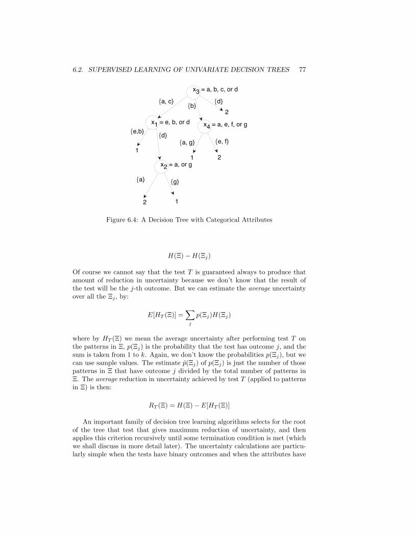
6.2. SUPERVISED LEARNING OF UNIVARIATE DECISION TREES 77
x3 = a, b, c, or d
a, cb
x1 = e, b, or d e,b
dx4 = a, e, f, or g
a, g e, f
x2 = a, or g
a g
1
2 1
1 2
d2
Figure 6.4: A Decision Tree with Categorical Attributes
H(Ξ)−H(Ξj)
Of course we cannot say that the test T is guaranteed always to produce thatamount of reduction in uncertainty because we don’t know that the result ofthe test will be the j-th outcome. But we can estimate the average uncertaintyover all the Ξj , by:
E[HT (Ξ)] =∑j
p(Ξj)H(Ξj)
where by HT (Ξ) we mean the average uncertainty after performing test T onthe patterns in Ξ, p(Ξj) is the probability that the test has outcome j, and thesum is taken from 1 to k. Again, we don’t know the probabilities p(Ξj), but wecan use sample values. The estimate p(Ξj) of p(Ξj) is just the number of thosepatterns in Ξ that have outcome j divided by the total number of patterns inΞ. The average reduction in uncertainty achieved by test T (applied to patternsin Ξ) is then:
RT (Ξ) = H(Ξ)− E[HT (Ξ)]
An important family of decision tree learning algorithms selects for the rootof the tree that test that gives maximum reduction of uncertainty, and thenapplies this criterion recursively until some termination condition is met (whichwe shall discuss in more detail later). The uncertainty calculations are particu-larly simple when the tests have binary outcomes and when the attributes have
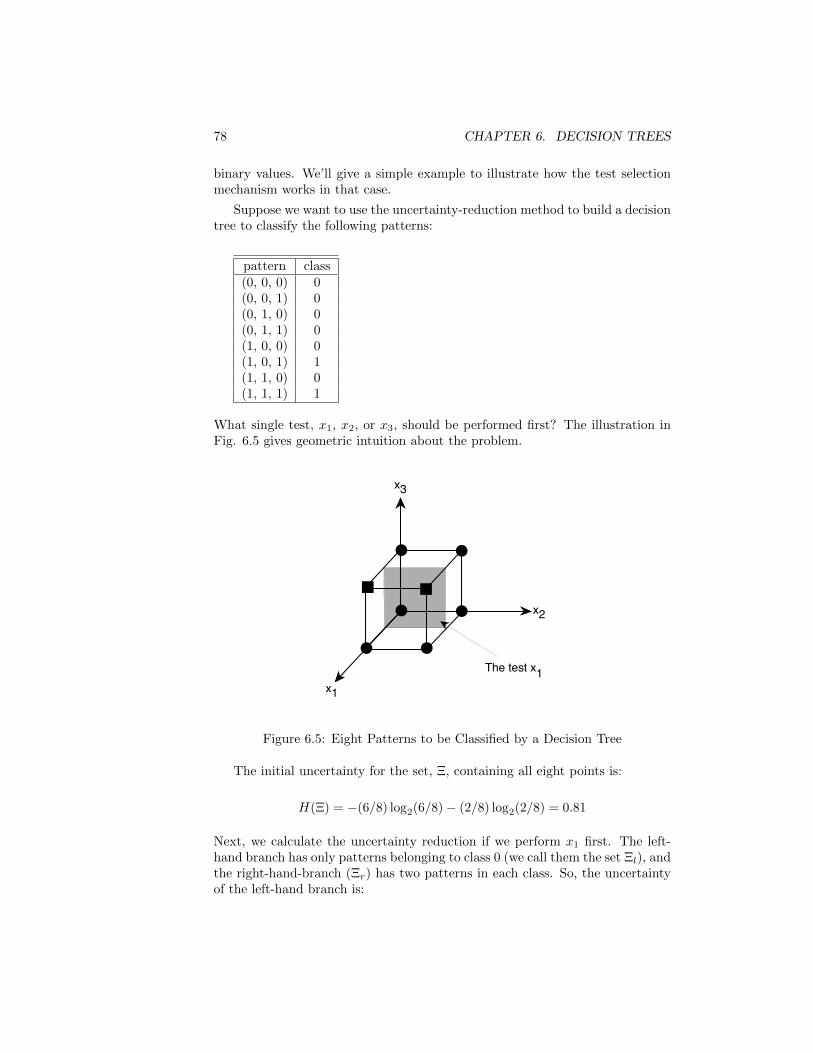
78 CHAPTER 6. DECISION TREES
binary values. We’ll give a simple example to illustrate how the test selectionmechanism works in that case.
Suppose we want to use the uncertainty-reduction method to build a decisiontree to classify the following patterns:
pattern class(0, 0, 0) 0(0, 0, 1) 0(0, 1, 0) 0(0, 1, 1) 0(1, 0, 0) 0(1, 0, 1) 1(1, 1, 0) 0(1, 1, 1) 1
What single test, x1, x2, or x3, should be performed first? The illustration inFig. 6.5 gives geometric intuition about the problem.
x1
x2
x3
The test x1
Figure 6.5: Eight Patterns to be Classified by a Decision Tree
The initial uncertainty for the set, Ξ, containing all eight points is:
H(Ξ) = −(6/8) log2(6/8)− (2/8) log2(2/8) = 0.81
Next, we calculate the uncertainty reduction if we perform x1 first. The left-hand branch has only patterns belonging to class 0 (we call them the set Ξl), andthe right-hand-branch (Ξr) has two patterns in each class. So, the uncertaintyof the left-hand branch is:
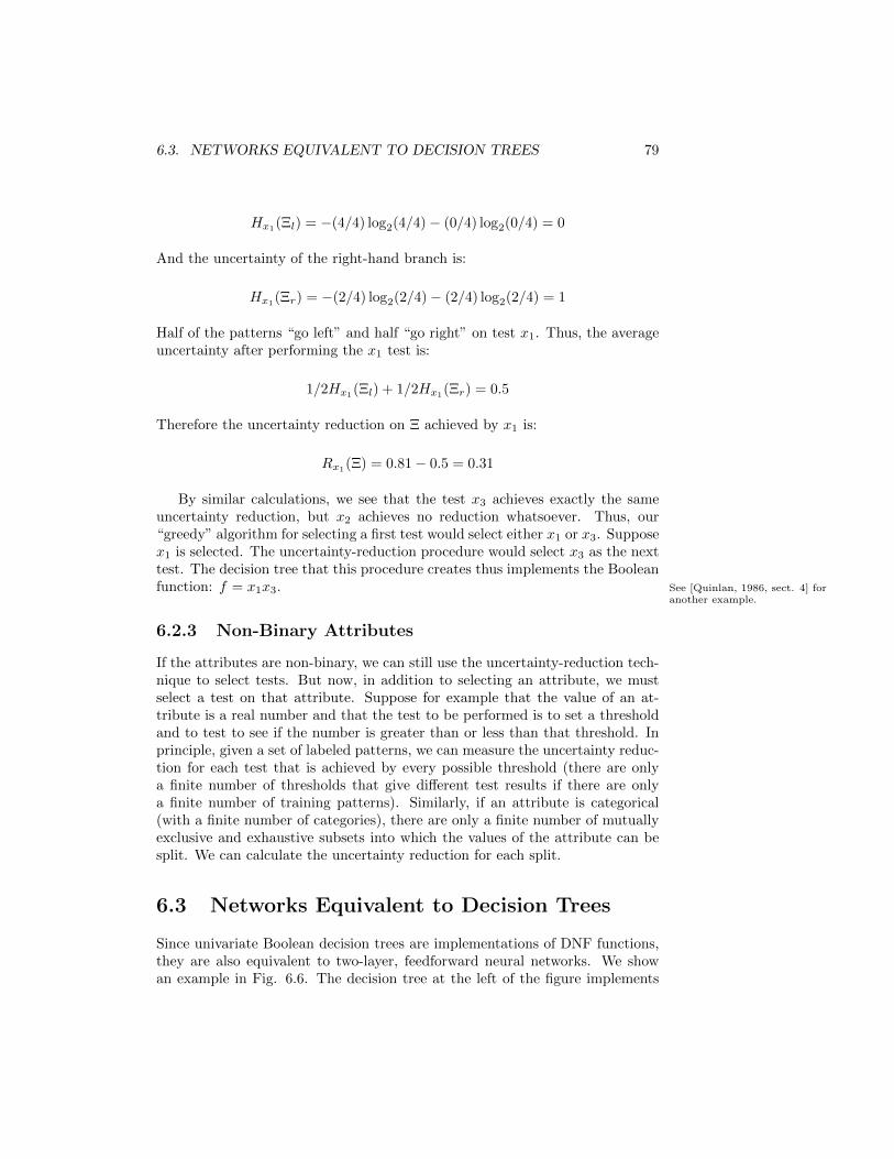
6.3. NETWORKS EQUIVALENT TO DECISION TREES 79
Hx1(Ξl) = −(4/4) log2(4/4)− (0/4) log2(0/4) = 0
And the uncertainty of the right-hand branch is:
Hx1(Ξr) = −(2/4) log2(2/4)− (2/4) log2(2/4) = 1
Half of the patterns “go left” and half “go right” on test x1. Thus, the averageuncertainty after performing the x1 test is:
1/2Hx1(Ξl) + 1/2Hx1
(Ξr) = 0.5
Therefore the uncertainty reduction on Ξ achieved by x1 is:
Rx1(Ξ) = 0.81− 0.5 = 0.31
By similar calculations, we see that the test x3 achieves exactly the sameuncertainty reduction, but x2 achieves no reduction whatsoever. Thus, our“greedy” algorithm for selecting a first test would select either x1 or x3. Supposex1 is selected. The uncertainty-reduction procedure would select x3 as the nexttest. The decision tree that this procedure creates thus implements the Booleanfunction: f = x1x3. See [Quinlan, 1986, sect. 4] for
another example.
6.2.3 Non-Binary Attributes
If the attributes are non-binary, we can still use the uncertainty-reduction tech-nique to select tests. But now, in addition to selecting an attribute, we mustselect a test on that attribute. Suppose for example that the value of an at-tribute is a real number and that the test to be performed is to set a thresholdand to test to see if the number is greater than or less than that threshold. Inprinciple, given a set of labeled patterns, we can measure the uncertainty reduc-tion for each test that is achieved by every possible threshold (there are onlya finite number of thresholds that give different test results if there are onlya finite number of training patterns). Similarly, if an attribute is categorical(with a finite number of categories), there are only a finite number of mutuallyexclusive and exhaustive subsets into which the values of the attribute can besplit. We can calculate the uncertainty reduction for each split.
6.3 Networks Equivalent to Decision Trees
Since univariate Boolean decision trees are implementations of DNF functions,they are also equivalent to two-layer, feedforward neural networks. We showan example in Fig. 6.6. The decision tree at the left of the figure implements
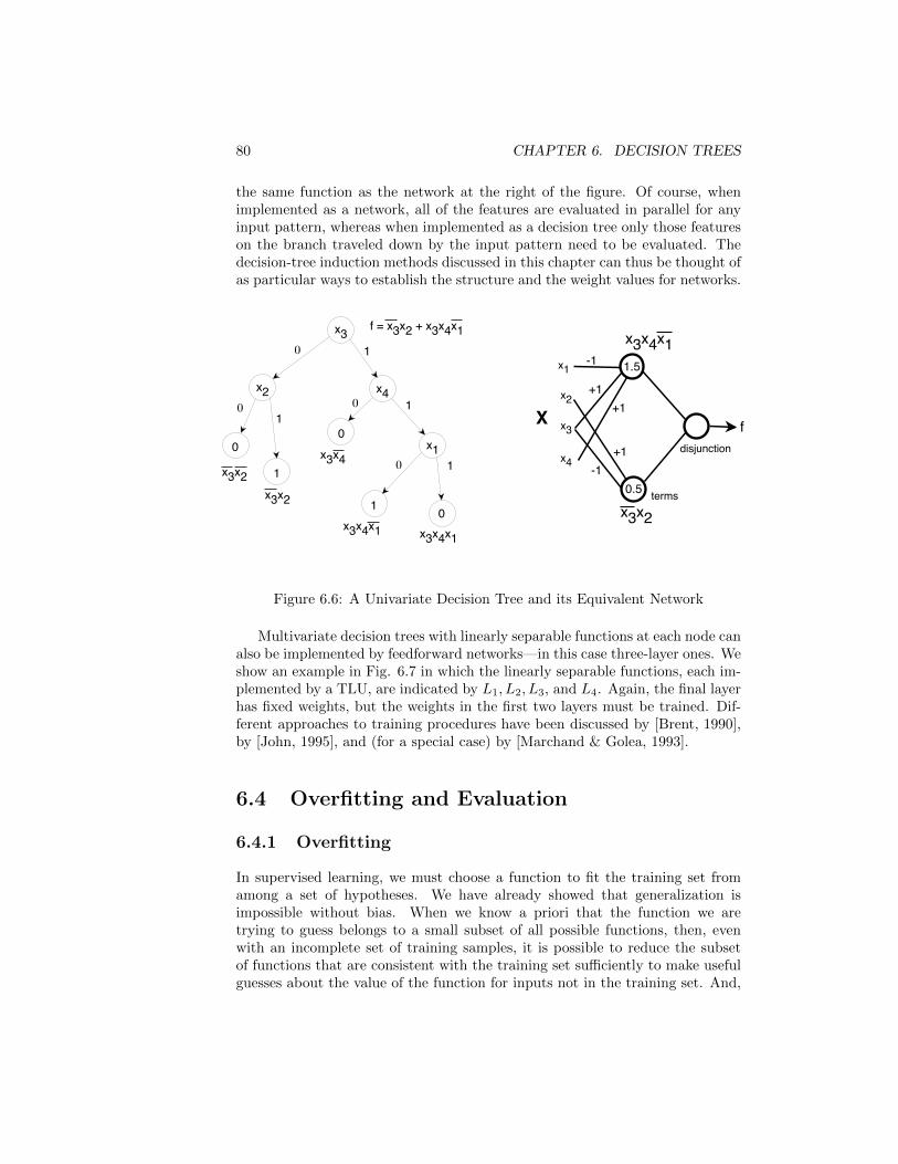
80 CHAPTER 6. DECISION TREES
the same function as the network at the right of the figure. Of course, whenimplemented as a network, all of the features are evaluated in parallel for anyinput pattern, whereas when implemented as a decision tree only those featureson the branch traveled down by the input pattern need to be evaluated. Thedecision-tree induction methods discussed in this chapter can thus be thought ofas particular ways to establish the structure and the weight values for networks.
X
x1
x2
x3
x4
terms
-1
+1
disjunction
x3x2
x3x4x1
+1
-1+1
f
1.5
0.5
x3
x2 x4
x1
10
1
1
0 0
0
1
x3x2x3x2
x3x4
x3x4x1 x3x4x1
f = x3x2 + x3x4x1
1
00
1 0
Figure 6.6: A Univariate Decision Tree and its Equivalent Network
Multivariate decision trees with linearly separable functions at each node canalso be implemented by feedforward networks—in this case three-layer ones. Weshow an example in Fig. 6.7 in which the linearly separable functions, each im-plemented by a TLU, are indicated by L1, L2, L3, and L4. Again, the final layerhas fixed weights, but the weights in the first two layers must be trained. Dif-ferent approaches to training procedures have been discussed by [Brent, 1990],by [John, 1995], and (for a special case) by [Marchand & Golea, 1993].
6.4 Overfitting and Evaluation
6.4.1 Overfitting
In supervised learning, we must choose a function to fit the training set fromamong a set of hypotheses. We have already showed that generalization isimpossible without bias. When we know a priori that the function we aretrying to guess belongs to a small subset of all possible functions, then, evenwith an incomplete set of training samples, it is possible to reduce the subsetof functions that are consistent with the training set sufficiently to make usefulguesses about the value of the function for inputs not in the training set. And,
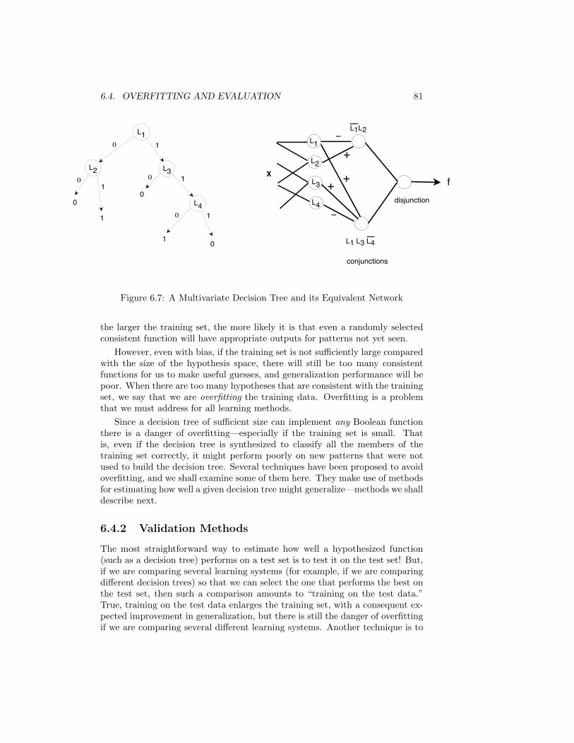
6.4. OVERFITTING AND EVALUATION 81
L1
L2 L3
L4
10
1
1
0 0
0
1
1
00
1 0
X
L1
L2
L3
L4
conjunctions
L1L2
L1 L3 L4
+
++disjunction
f
Figure 6.7: A Multivariate Decision Tree and its Equivalent Network
the larger the training set, the more likely it is that even a randomly selectedconsistent function will have appropriate outputs for patterns not yet seen.
However, even with bias, if the training set is not sufficiently large comparedwith the size of the hypothesis space, there will still be too many consistentfunctions for us to make useful guesses, and generalization performance will bepoor. When there are too many hypotheses that are consistent with the trainingset, we say that we are overfitting the training data. Overfitting is a problemthat we must address for all learning methods.
Since a decision tree of sufficient size can implement any Boolean functionthere is a danger of overfitting—especially if the training set is small. Thatis, even if the decision tree is synthesized to classify all the members of thetraining set correctly, it might perform poorly on new patterns that were notused to build the decision tree. Several techniques have been proposed to avoidoverfitting, and we shall examine some of them here. They make use of methodsfor estimating how well a given decision tree might generalize—methods we shalldescribe next.
6.4.2 Validation Methods
The most straightforward way to estimate how well a hypothesized function(such as a decision tree) performs on a test set is to test it on the test set! But,if we are comparing several learning systems (for example, if we are comparingdifferent decision trees) so that we can select the one that performs the best onthe test set, then such a comparison amounts to “training on the test data.”True, training on the test data enlarges the training set, with a consequent ex-pected improvement in generalization, but there is still the danger of overfittingif we are comparing several different learning systems. Another technique is to
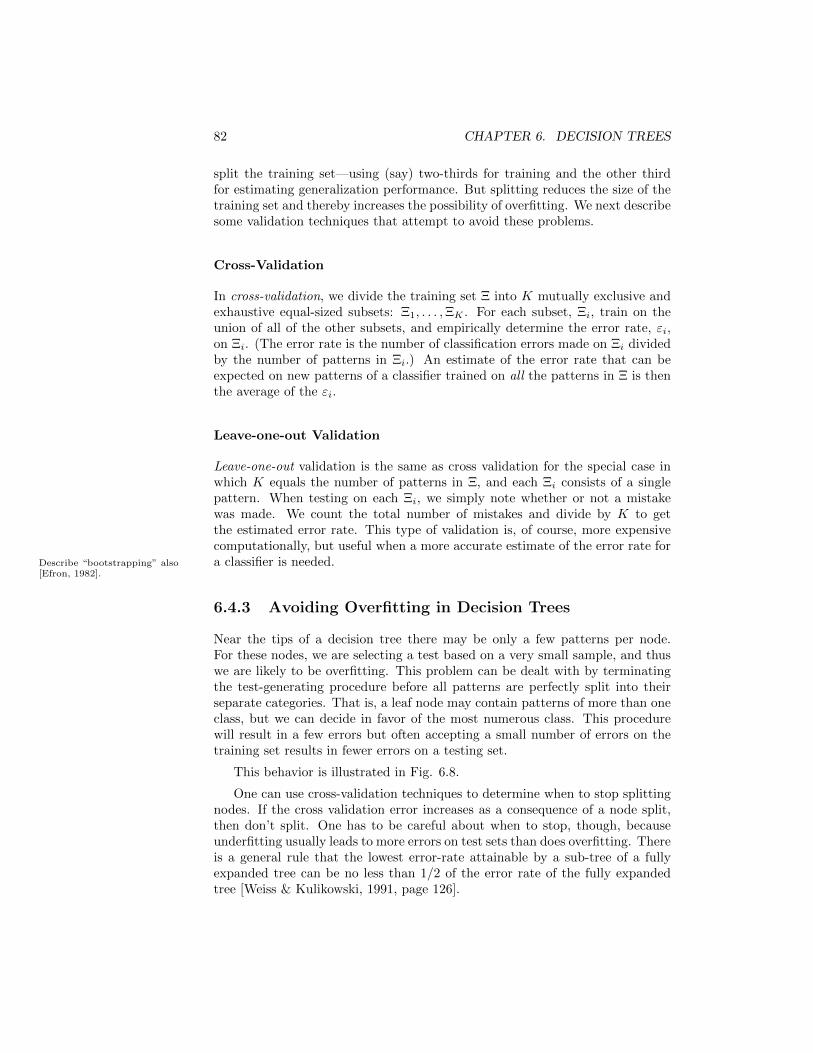
82 CHAPTER 6. DECISION TREES
split the training set—using (say) two-thirds for training and the other thirdfor estimating generalization performance. But splitting reduces the size of thetraining set and thereby increases the possibility of overfitting. We next describesome validation techniques that attempt to avoid these problems.
Cross-Validation
In cross-validation, we divide the training set Ξ into K mutually exclusive andexhaustive equal-sized subsets: Ξ1, . . . ,ΞK . For each subset, Ξi, train on theunion of all of the other subsets, and empirically determine the error rate, εi,on Ξi. (The error rate is the number of classification errors made on Ξi dividedby the number of patterns in Ξi.) An estimate of the error rate that can beexpected on new patterns of a classifier trained on all the patterns in Ξ is thenthe average of the εi.
Leave-one-out Validation
Leave-one-out validation is the same as cross validation for the special case inwhich K equals the number of patterns in Ξ, and each Ξi consists of a singlepattern. When testing on each Ξi, we simply note whether or not a mistakewas made. We count the total number of mistakes and divide by K to getthe estimated error rate. This type of validation is, of course, more expensivecomputationally, but useful when a more accurate estimate of the error rate fora classifier is needed.Describe “bootstrapping” also
[Efron, 1982].
6.4.3 Avoiding Overfitting in Decision Trees
Near the tips of a decision tree there may be only a few patterns per node.For these nodes, we are selecting a test based on a very small sample, and thuswe are likely to be overfitting. This problem can be dealt with by terminatingthe test-generating procedure before all patterns are perfectly split into theirseparate categories. That is, a leaf node may contain patterns of more than oneclass, but we can decide in favor of the most numerous class. This procedurewill result in a few errors but often accepting a small number of errors on thetraining set results in fewer errors on a testing set.
This behavior is illustrated in Fig. 6.8.
One can use cross-validation techniques to determine when to stop splittingnodes. If the cross validation error increases as a consequence of a node split,then don’t split. One has to be careful about when to stop, though, becauseunderfitting usually leads to more errors on test sets than does overfitting. Thereis a general rule that the lowest error-rate attainable by a sub-tree of a fullyexpanded tree can be no less than 1/2 of the error rate of the fully expandedtree [Weiss & Kulikowski, 1991, page 126].
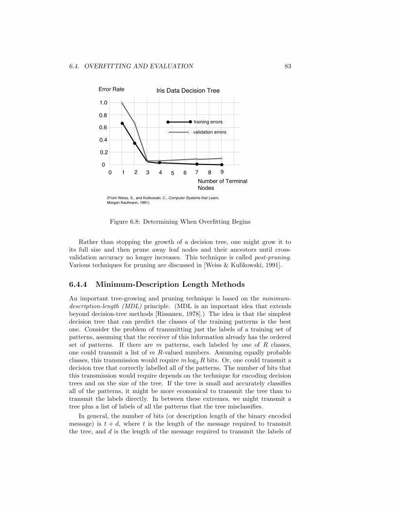
6.4. OVERFITTING AND EVALUATION 83
(From Weiss, S., and Kulikowski, C., Computer Systems that Learn,Morgan Kaufmann, 1991)
training errors
validation errors
1 2 3 4 5 6 7 8 9
0.2
0.4
0.6
0.8
1.0
00
Error Rate
Number of TerminalNodes
Iris Data Decision Tree
Figure 6.8: Determining When Overfitting Begins
Rather than stopping the growth of a decision tree, one might grow it toits full size and then prune away leaf nodes and their ancestors until cross-validation accuracy no longer increases. This technique is called post-pruning.Various techniques for pruning are discussed in [Weiss & Kulikowski, 1991].
6.4.4 Minimum-Description Length Methods
An important tree-growing and pruning technique is based on the minimum-description-length (MDL) principle. (MDL is an important idea that extendsbeyond decision-tree methods [Rissanen, 1978].) The idea is that the simplestdecision tree that can predict the classes of the training patterns is the bestone. Consider the problem of transmitting just the labels of a training set ofpatterns, assuming that the receiver of this information already has the orderedset of patterns. If there are m patterns, each labeled by one of R classes,one could transmit a list of m R-valued numbers. Assuming equally probableclasses, this transmission would require m log2R bits. Or, one could transmit adecision tree that correctly labelled all of the patterns. The number of bits thatthis transmission would require depends on the technique for encoding decisiontrees and on the size of the tree. If the tree is small and accurately classifiesall of the patterns, it might be more economical to transmit the tree than totransmit the labels directly. In between these extremes, we might transmit atree plus a list of labels of all the patterns that the tree misclassifies.
In general, the number of bits (or description length of the binary encodedmessage) is t + d, where t is the length of the message required to transmitthe tree, and d is the length of the message required to transmit the labels of
84 CHAPTER 6. DECISION TREES
the patterns misclassified by the tree. In a sense, that tree associated with thesmallest value of t + d is the best or most economical tree. The MDL methodis one way of adhering to the Occam’s razor principle.
Quinlan and Rivest [Quinlan & Rivest, 1989] have proposed techniques forencoding decision trees and lists of exception labels and for calculating thedescription length (t+d) of these trees and labels. They then use the descriptionlength as a measure of quality of a tree in two ways:
a. In growing a tree, they use the reduction in description length to selecttests (instead of reduction in uncertainty).
b. In pruning a tree after it has been grown to zero error, they prune awaythose nodes (starting at the tips) that achieve a decrease in the descriptionlength.
These techniques compare favorably with the uncertainty-reduction method,although they are quite sensitive to the coding schemes used.
6.4.5 Noise in Data
Noise in the data means that one must inevitably accept some number oferrors—depending on the noise level. Refusal to tolerate errors on the trainingset when there is noise leads to the problem of “fitting the noise.” Dealing withnoise, then, requires accepting some errors at the leaf nodes just as does thefact that there are a small number of patterns at leaf nodes.
6.5 The Problem of Replicated Subtrees
Decision trees are not the most economical means of implementing some Booleanfunctions. Consider, for example, the function f = x1x2 +x3x4. A decision treefor this function is shown in Fig. 6.9. Notice the replicated subtrees showncircled. The DNF-form equivalent to the function implemented by this decisiontree is f = x1x2 + x1x2x3x4 + x1x3x4. This DNF form is non-minimal (in thenumber of disjunctions) and is equivalent to f = x1x2 + x3x4.
The need for replication means that it takes longer to learn the tree andthat subtrees replicated further down the tree must be learned using a smallertraining subset. This problem is sometimes called the fragmentation problem.
Several approaches might be suggested for dealing with fragmenta-tion. One is to attempt to build a decision graph instead of a tree[Oliver, Dowe, & Wallace, 1992, Kohavi, 1994]. A decision graph that imple-ments the same decisions as that of the decision tree of Fig. 6.9 is shown in Fig.6.10.
Another approach is to use multivariate (rather than univariate tests at eachnode). In our example of learning f = x1x2 + x3x4, if we had a test for x1x2
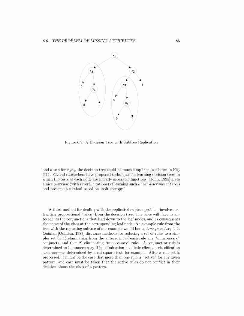
6.6. THE PROBLEM OF MISSING ATTRIBUTES 85
x1
x3 x2
10x4
0 1
x3
0x4
0 1
Figure 6.9: A Decision Tree with Subtree Replication
and a test for x3x4, the decision tree could be much simplified, as shown in Fig.6.11. Several researchers have proposed techniques for learning decision trees inwhich the tests at each node are linearly separable functions. [John, 1995] givesa nice overview (with several citations) of learning such linear discriminant treesand presents a method based on “soft entropy.”
A third method for dealing with the replicated subtree problem involves ex-tracting propositional “rules” from the decision tree. The rules will have as an-tecedents the conjunctions that lead down to the leaf nodes, and as consequentsthe name of the class at the corresponding leaf node. An example rule from thetree with the repeating subtree of our example would be: x1∧¬x2∧x3∧x4 ⊃ 1.Quinlan [Quinlan, 1987] discusses methods for reducing a set of rules to a sim-pler set by 1) eliminating from the antecedent of each rule any “unnecessary”conjuncts, and then 2) eliminating “unnecessary” rules. A conjunct or rule isdetermined to be unnecessary if its elimination has little effect on classificationaccuracy—as determined by a chi-square test, for example. After a rule set isprocessed, it might be the case that more than one rule is “active” for any givenpattern, and care must be taken that the active rules do not conflict in theirdecision about the class of a pattern.
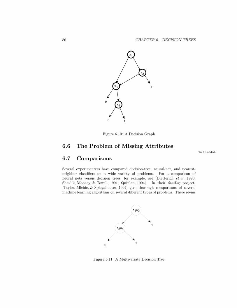
86 CHAPTER 6. DECISION TREES
x1
x3
x2
1
0x4
0 1
Figure 6.10: A Decision Graph
6.6 The Problem of Missing AttributesTo be added.
6.7 Comparisons
Several experimenters have compared decision-tree, neural-net, and nearest-neighbor classifiers on a wide variety of problems. For a comparison ofneural nets versus decision trees, for example, see [Dietterich, et al., 1990,Shavlik, Mooney, & Towell, 1991, Quinlan, 1994]. In their StatLog project,[Taylor, Michie, & Spiegalhalter, 1994] give thorough comparisons of severalmachine learning algorithms on several different types of problems. There seems
x1x2
1
0
x3x4
1
Figure 6.11: A Multivariate Decision Tree

6.8. BIBLIOGRAPHICAL AND HISTORICAL REMARKS 87
to be no single type of classifier that is best for all problems. And, there donot seem to be any general conclusions that would enable one to say whichclassifier method is best for which sorts of classification problems, although[Quinlan, 1994] does provide some intuition about properties of problems thatmight render them ill suited for decision trees, on the one hand, or backpropa-gation, on the other.
6.8 Bibliographical and Historical RemarksTo be added.

88 CHAPTER 6. DECISION TREES
Chapter 7
Inductive LogicProgramming
There are many different representational forms for functions of input vari-ables. So far, we have seen (Boolean) algebraic expressions, decision trees, andneural networks, plus other computational mechanisms such as techniques forcomputing nearest neighbors. Of course, the representation most importantin computer science is a computer program. For example, a Lisp predicate ofbinary-valued inputs computes a Boolean function of those inputs. Similarly, alogic program (whose ordinary application is to compute bindings for variables)can also be used simply to decide whether or not a predicate has value True(T) or False (F). For example, the Boolean exclusive-or (odd parity) functionof two variables can be computed by the following logic program:
Parity(x,y) :- True(x), ¬ True(y)
:- True(y), ¬ True(x)
We follow Prolog syntax (see, for example, [Mueller & Page, 1988]), except thatour convention is to write variables as strings beginning with lower-case lettersand predicates as strings beginning with upper-case letters. The unary function“True” returns T if and only if the value of its argument is T . (We now thinkof Boolean functions and arguments as having values of T and F instead of 0and 1.) Programs will be written in “typewriter” font.
In this chapter, we consider the matter of learning logic programs givena set of variable values for which the logic program should return T (thepositive instances) and a set of variable values for which it should returnF (the negative instances). The subspecialty of machine learning that dealswith learning logic programs is called inductive logic programming (ILP)[Lavrac & Dzeroski, 1994]. As with any learning problem, this one can be quitecomplex and intractably difficult unless we constrain it with biases of some sort.
89
90 CHAPTER 7. INDUCTIVE LOGIC PROGRAMMING
In ILP, there are a variety of possible biases (called language biases). One mightrestrict the program to Horn clauses, not allow recursion, not allow functions,and so on.
As an example of an ILP problem, suppose we are trying to induce a func-tion Nonstop(x,y), that is to have value T for pairs of cities connected by anon-stop air flight and F for all other pairs of cities. We are given a training setconsisting of positive and negative examples. As positive examples, we mighthave (A,B), (A, A1), and some other pairs; as negative examples, we mighthave (A1, A2), and some other pairs. In ILP, we usually have additional infor-mation about the examples, called “background knowledge.” In our air-flightproblem, the background information might be such ground facts as Hub(A),Hub(B), Satellite(A1,A), plus others. (Hub(A) is intended to mean that thecity denoted by A is a hub city, and Satellite(A1,A) is intended to mean thatthe city denoted by A1 is a satellite of the city denoted by A.) From these train-ing facts, we want to induce a program Nonstop(x,y), written in terms of thebackground relations Hub and Satellite, that has value T for all the positiveinstances and has value F for all the negative instances. Depending on the exactset of examples, we might induce the program:
Nonstop(x,y) :- Hub(x), Hub(y)
:- Satellite(x,y)
:- Satellite(y,x)
which would have value T if both of the two cities were hub cities or if one werea satellite of the other. As with other learning problems, we want the inducedprogram to generalize well; that is, if presented with arguments not representedin the training set (but for which we have the needed background knowledge),we would like the function to guess well.
7.1 Notation and Definitions
In evaluating logic programs in ILP, we implicitly append the background factsto the program and adopt the usual convention that a program has value T fora set of inputs if and only if the program interpreter returns T when actuallyrunning the program (with background facts appended) on those inputs; oth-erwise it has value F . Using the given background facts, the program abovewould return T for input (A, A1), for example. If a logic program, π, returnsT for a set of arguments X, we say that the program covers the arguments andwrite covers(π,X). Following our terminology introduced in connection withversion spaces, we will say that a program is sufficient if it covers all of thepositive instances and that it is necessary if it does not cover any of the neg-ative instances. (That is, a program implements a sufficient condition that atraining instance is positive if it covers all of the positive training instances; it
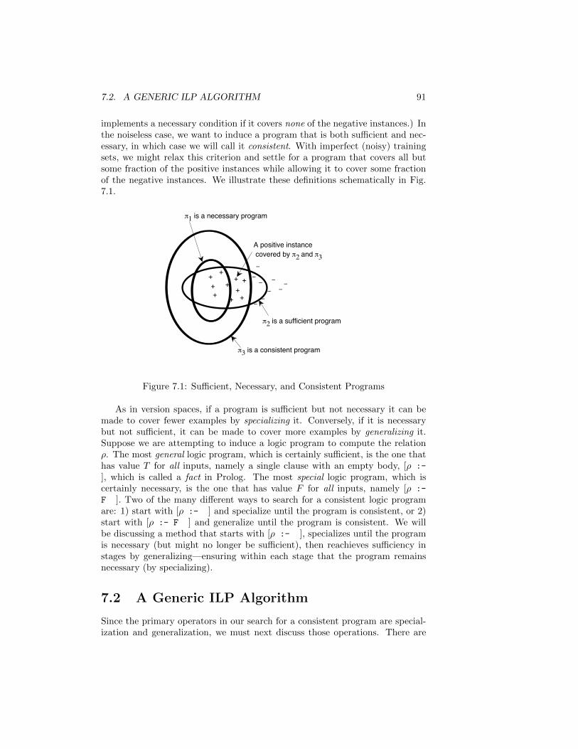
7.2. A GENERIC ILP ALGORITHM 91
implements a necessary condition if it covers none of the negative instances.) Inthe noiseless case, we want to induce a program that is both sufficient and nec-essary, in which case we will call it consistent. With imperfect (noisy) trainingsets, we might relax this criterion and settle for a program that covers all butsome fraction of the positive instances while allowing it to cover some fractionof the negative instances. We illustrate these definitions schematically in Fig.7.1.
1 is a necessary program
2 is a sufficient program
3 is a consistent program
+
+
++
++
+
++
+
A positive instance covered by 2 and 3
Figure 7.1: Sufficient, Necessary, and Consistent Programs
As in version spaces, if a program is sufficient but not necessary it can bemade to cover fewer examples by specializing it. Conversely, if it is necessarybut not sufficient, it can be made to cover more examples by generalizing it.Suppose we are attempting to induce a logic program to compute the relationρ. The most general logic program, which is certainly sufficient, is the one thathas value T for all inputs, namely a single clause with an empty body, [ρ :-
], which is called a fact in Prolog. The most special logic program, which iscertainly necessary, is the one that has value F for all inputs, namely [ρ :-
F ]. Two of the many different ways to search for a consistent logic programare: 1) start with [ρ :- ] and specialize until the program is consistent, or 2)start with [ρ :- F ] and generalize until the program is consistent. We willbe discussing a method that starts with [ρ :- ], specializes until the programis necessary (but might no longer be sufficient), then reachieves sufficiency instages by generalizing—ensuring within each stage that the program remainsnecessary (by specializing).
7.2 A Generic ILP Algorithm
Since the primary operators in our search for a consistent program are special-ization and generalization, we must next discuss those operations. There are
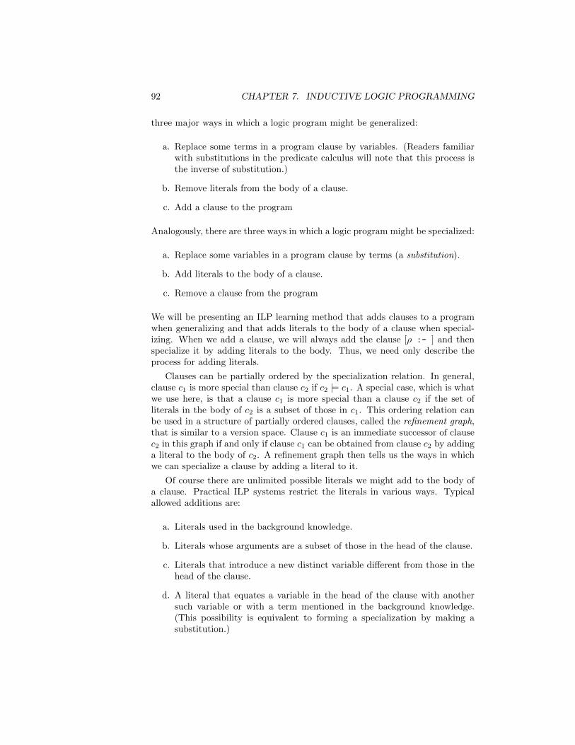
92 CHAPTER 7. INDUCTIVE LOGIC PROGRAMMING
three major ways in which a logic program might be generalized:
a. Replace some terms in a program clause by variables. (Readers familiarwith substitutions in the predicate calculus will note that this process isthe inverse of substitution.)
b. Remove literals from the body of a clause.
c. Add a clause to the program
Analogously, there are three ways in which a logic program might be specialized:
a. Replace some variables in a program clause by terms (a substitution).
b. Add literals to the body of a clause.
c. Remove a clause from the program
We will be presenting an ILP learning method that adds clauses to a programwhen generalizing and that adds literals to the body of a clause when special-izing. When we add a clause, we will always add the clause [ρ :- ] and thenspecialize it by adding literals to the body. Thus, we need only describe theprocess for adding literals.
Clauses can be partially ordered by the specialization relation. In general,clause c1 is more special than clause c2 if c2 |= c1. A special case, which is whatwe use here, is that a clause c1 is more special than a clause c2 if the set ofliterals in the body of c2 is a subset of those in c1. This ordering relation canbe used in a structure of partially ordered clauses, called the refinement graph,that is similar to a version space. Clause c1 is an immediate successor of clausec2 in this graph if and only if clause c1 can be obtained from clause c2 by addinga literal to the body of c2. A refinement graph then tells us the ways in whichwe can specialize a clause by adding a literal to it.
Of course there are unlimited possible literals we might add to the body ofa clause. Practical ILP systems restrict the literals in various ways. Typicalallowed additions are:
a. Literals used in the background knowledge.
b. Literals whose arguments are a subset of those in the head of the clause.
c. Literals that introduce a new distinct variable different from those in thehead of the clause.
d. A literal that equates a variable in the head of the clause with anothersuch variable or with a term mentioned in the background knowledge.(This possibility is equivalent to forming a specialization by making asubstitution.)
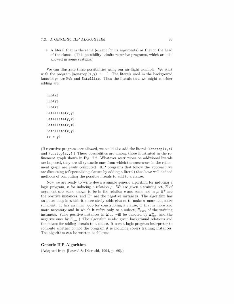
7.2. A GENERIC ILP ALGORITHM 93
e. A literal that is the same (except for its arguments) as that in the headof the clause. (This possibility admits recursive programs, which are dis-allowed in some systems.)
We can illustrate these possibilities using our air-flight example. We startwith the program [Nonstop(x,y) :- ]. The literals used in the backgroundknowledge are Hub and Satellite. Thus the literals that we might consideradding are:
Hub(x)
Hub(y)
Hub(z)
Satellite(x,y)
Satellite(y,x)
Satellite(x,z)
Satellite(z,y)
(x = y)
(If recursive programs are allowed, we could also add the literals Nonstop(x,z)and Nonstop(z,y).) These possibilities are among those illustrated in the re-finement graph shown in Fig. 7.2. Whatever restrictions on additional literalsare imposed, they are all syntactic ones from which the successors in the refine-ment graph are easily computed. ILP programs that follow the approach weare discussing (of specializing clauses by adding a literal) thus have well definedmethods of computing the possible literals to add to a clause.
Now we are ready to write down a simple generic algorithm for inducing alogic program, π for inducing a relation ρ. We are given a training set, Ξ ofargument sets some known to be in the relation ρ and some not in ρ; Ξ+ arethe positive instances, and Ξ− are the negative instances. The algorithm hasan outer loop in which it successively adds clauses to make π more and moresufficient. It has an inner loop for constructing a clause, c, that is more andmore necessary and in which it refers only to a subset, Ξcur, of the traininginstances. (The positive instances in Ξcur will be denoted by Ξ+
cur, and thenegative ones by Ξ−cur.) The algorithm is also given background relations andthe means for adding literals to a clause. It uses a logic program interpreter tocompute whether or not the program it is inducing covers training instances.The algorithm can be written as follows:
Generic ILP Algorithm
(Adapted from [Lavrac & Dzeroski, 1994, p. 60].)
94 CHAPTER 7. INDUCTIVE LOGIC PROGRAMMING
Nonstop(x,y) :-
Nonstop(x,y) :- Hub(x)
Nonstop(x,y) :- Satellite(x,y)
Nonstop(x,y) :- (x = y)
. . .
. . .
. . . . . .
Nonstop(x,y) :- Hub(x), Hub(y)
. . .
. . .
. . .
Figure 7.2: Part of a Refinement Graph
Initialize Ξcur := Ξ.Initialize π := empty set of clauses.repeat [The outer loop works to make π sufficient.]
Initialize c := ρ : − .repeat [The inner loop makes c necessary.]
Select a literal l to add to c. [This is a nondeterministic choice point.]Assign c := c, l.
until c is necessary. [That is, until c covers no negative instances in Ξcur.]Assign π := π, c. [We add the clause c to the program.]Assign Ξcur := Ξcur − (the positive instances in Ξcur covered by π).
until π is sufficient.
(The termination tests for the inner and outer loops can be relaxed as appro-priate for the case of noisy instances.)
7.3 An Example
We illustrate how the algorithm works by returning to our example of airlineflights. Consider the portion of an airline route map, shown in Fig. 7.3. CitiesA, B, and C are “hub” cities, and we know that there are nonstop flights betweenall hub cities (even those not shown on this portion of the route map). The other
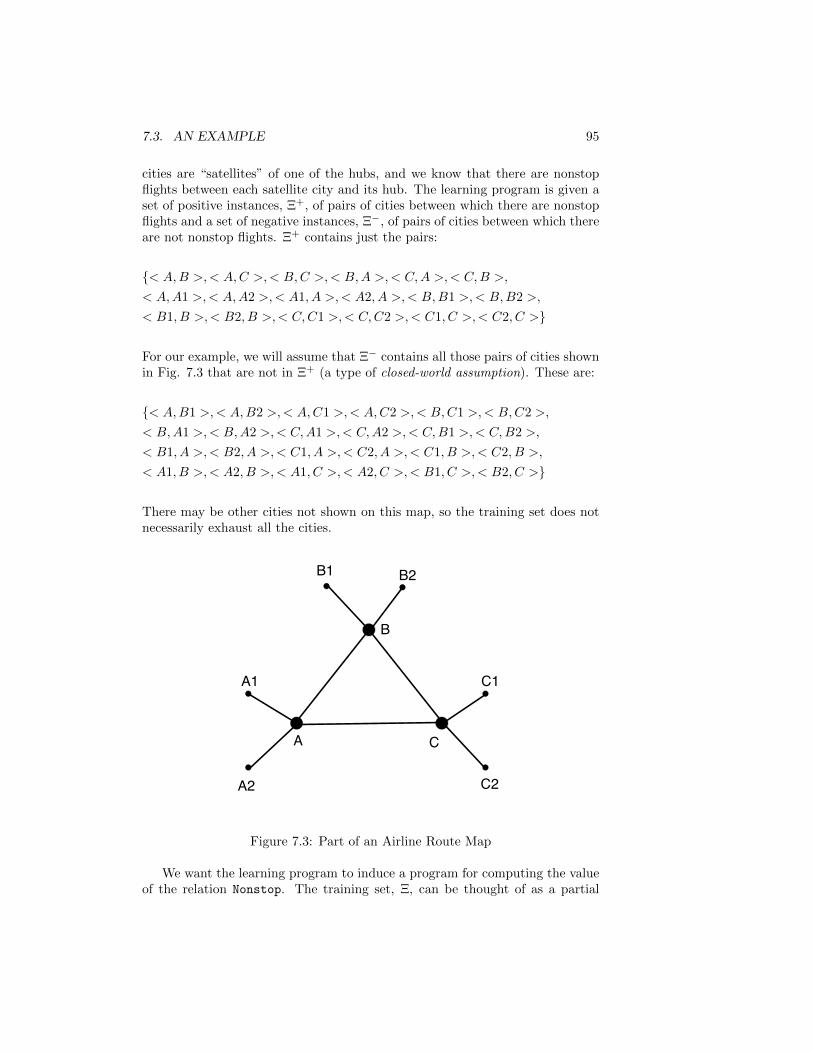
7.3. AN EXAMPLE 95
cities are “satellites” of one of the hubs, and we know that there are nonstopflights between each satellite city and its hub. The learning program is given aset of positive instances, Ξ+, of pairs of cities between which there are nonstopflights and a set of negative instances, Ξ−, of pairs of cities between which thereare not nonstop flights. Ξ+ contains just the pairs:
< A,B >,< A,C >,< B,C >,< B,A >,< C,A >,< C,B >,
< A,A1 >,< A,A2 >,< A1, A >,< A2, A >,< B,B1 >,< B,B2 >,
< B1, B >,< B2, B >,< C,C1 >,< C,C2 >,< C1, C >,< C2, C >
For our example, we will assume that Ξ− contains all those pairs of cities shownin Fig. 7.3 that are not in Ξ+ (a type of closed-world assumption). These are:
< A,B1 >,< A,B2 >,< A,C1 >,< A,C2 >,< B,C1 >,< B,C2 >,
< B,A1 >,< B,A2 >,< C,A1 >,< C,A2 >,< C,B1 >,< C,B2 >,
< B1, A >,< B2, A >,< C1, A >,< C2, A >,< C1, B >,< C2, B >,
< A1, B >,< A2, B >,< A1, C >,< A2, C >,< B1, C >,< B2, C >
There may be other cities not shown on this map, so the training set does notnecessarily exhaust all the cities.
A
B
C
C1
C2
B1 B2
A1
A2
Figure 7.3: Part of an Airline Route Map
We want the learning program to induce a program for computing the valueof the relation Nonstop. The training set, Ξ, can be thought of as a partial
96 CHAPTER 7. INDUCTIVE LOGIC PROGRAMMING
description of this relation in extensional form—it explicitly names some pairsin the relation and some pairs not in the relation. We desire to learn theNonstop relation as a logic program in terms of the background relations, Huband Satellite, which are also given in extensional form. Doing so will give usa more compact, intensional, description of the relation, and this descriptioncould well generalize usefully to other cities not mentioned in the map.
We assume the learning program has the following extensional definitions ofthe relations Hub and Satellite:
Hub
< A >,< B >,< C >
All other cities mentioned in the map are assumed not in the relation Hub. Wewill use the notation Hub(x) to express that the city named x is in the relationHub.
Satellite
< A1, A,>,< A2, A >,< B1, B >,< B2, B >,< C1, C >,< C2, C >
All other pairs of cities mentioned in the map are not in the relation Satellite.We will use the notation Satellite(x,y) to express that the pair < x, y > isin the relation Satellite.
Knowing that the predicate Nonstop is a two-place predicate, the inner loopof our algorithm initializes the first clause to Nonstop(x,y) :- . This clauseis not necessary because it covers all the negative examples (since it covers allexamples). So we must add a literal to its (empty) body. Suppose (selectinga literal from the refinement graph) the algorithm adds Hub(x). The followingpositive instances in Ξ are covered by Nonstop(x,y) :- Hub(x):
< A,B >,< A,C >,< B,C >,< B,A >,< C,A >,< C,B >,
< A,A1 >,< A,A2 >,< B,B1 >,< B,B2 >,< C,C1 >,< C,C2 >
To compute this covering, we interpret the logic program Nonstop(x,y) :-
Hub(x) for all pairs of cities in Ξ, using the pairs given in the backgroundrelation Hub as ground facts. The following negative instances are also covered:
7.3. AN EXAMPLE 97
< A,B1 >,< A,B2 >,< A,C1 >,< A,C2 >,< C,A1 >,< C,A2 >,
< C,B1 >,< C,B2 >,< B,A1 >,< B,A2 >,< B,C1 >,< B,C2 >
Thus, the clause is not yet necessary and another literal must be added. Sup-pose we next add Hub(y). The following positive instances are covered byNonstop(x,y) :- Hub(x), Hub(y):
< A,B >,< A,C >,< B,C >,< B,A >,< C,A >,< C,B >
There are no longer any negative instances in Ξ covered so the clauseNonstop(x,y) :- Hub(x), Hub(y) is necessary, and we can terminate the firstpass through the inner loop.
But the program, π, consisting of just this clause is not sufficient. Thesepositive instances are not covered by the clause:
< A,A1 >,< A,A2 >,< A1, A >,< A2, A >,< B,B1 >,< B,B2 >,
< B1, B >,< B2, B >,< C,C1 >,< C,C2 >,< C1, C >,< C2, C >
The positive instances that were covered by Nonstop(x,y) :- Hub(x), Hub(y)
are removed from Ξ to form the Ξcur to be used in the next pass through theinner loop. Ξcur consists of all the negative instances in Ξ plus the positiveinstances (listed above) that are not yet covered. In order to attempt to coverthem, the inner loop creates another clause c, initially set to Nonstop(x,y)
:- . This clause covers all the negative instances, and so we must add liter-als to make it necessary. Suppose we add the literal Satellite(x,y). Theclause Nonstop(x,y) :- Satellite(x,y) covers no negative instances, so it isnecessary. It does cover the following positive instances in Ξcur:
< A1, A >,< A2, A >,< B1, B >,< B2, B >,< C1, C >,< C2, C >
These instances are removed from Ξcur for the next pass through the inner loop.The program now contains two clauses:
Nonstop(x,y) :- Hub(x), Hub(y)
:- Satellite(x,y)
This program is not yet sufficient since it does not cover the following positiveinstances:
< A,A1 >,< A,A2 >,< B,B1 >,< B,B2 >,< C,C1 >,< C,C2 >
98 CHAPTER 7. INDUCTIVE LOGIC PROGRAMMING
During the next pass through the inner loop, we add the clause Nonstop(x,y):- Satellite(y,x). This clause is necessary, and since the program containingall three clauses is now sufficient, the procedure terminates with:
Nonstop(x,y) :- Hub(x), Hub(y)
:- Satellite(x,y)
:- Satellite(y,x)
Since each clause is necessary, and the whole program is sufficient, the pro-gram is also consistent with all instances of the training set. Note that thisprogram can be applied (perhaps with good generalization) to other cities be-sides those in our partial map—so long as we can evaluate the relations Hub andSatellite for these other cities. In the next section, we show how the techniquecan be extended to use recursion on the relation we are inducing. With thatextension, the method can be used to induce more general logic programs.
7.4 Inducing Recursive Programs
To induce a recursive program, we allow the addition of a literal having thesame predicate letter as that in the head of the clause. Various mechanismsmust be used to ensure that such a program will terminate; one such is to makesure that the new literal has different variables than those in the head literal.The process is best illustrated with another example. Our example continuesthe one using the airline map, but we make the map somewhat simpler in orderto reduce the size of the extensional relations used. Consider the map shownin Fig. 7.4. Again, B and C are hub cities, B1 and B2 are satellites of B, C1and C2 are satellites of C. We have introduced two new cities, B3 and C3. Noflights exist between these cities and any other cities—perhaps there are onlybus routes as shown by the grey lines in the map.
We now seek to learn a program for Canfly(x,y) that covers only thosepairs of cities that can be reached by one or more nonstop flights. The relationCanfly is satisfied by the following pairs of postive instances:
< B1, B >,< B1, B2 >,< B1, C >,< B1, C1 >,< B1, C2 >,
< B,B1 >,< B2, B1 >,< C,B1 >,< C1, B1 >,< C2, B1 >,
< B2, B >,< B2, C >,< B2, C1 >,< B2, C2 >,< B,B2 >,
< C,B2 >,< C1, B2 >,< C2, B2 >,< B,C >,< B,C1 >,
< B,C2 >,< C,B >,< C1, B >,< C2, B >,< C,C1 >,
< C,C2 >,< C1, C >,< C2, C >,< C1, C2 >,< C2, C1 >
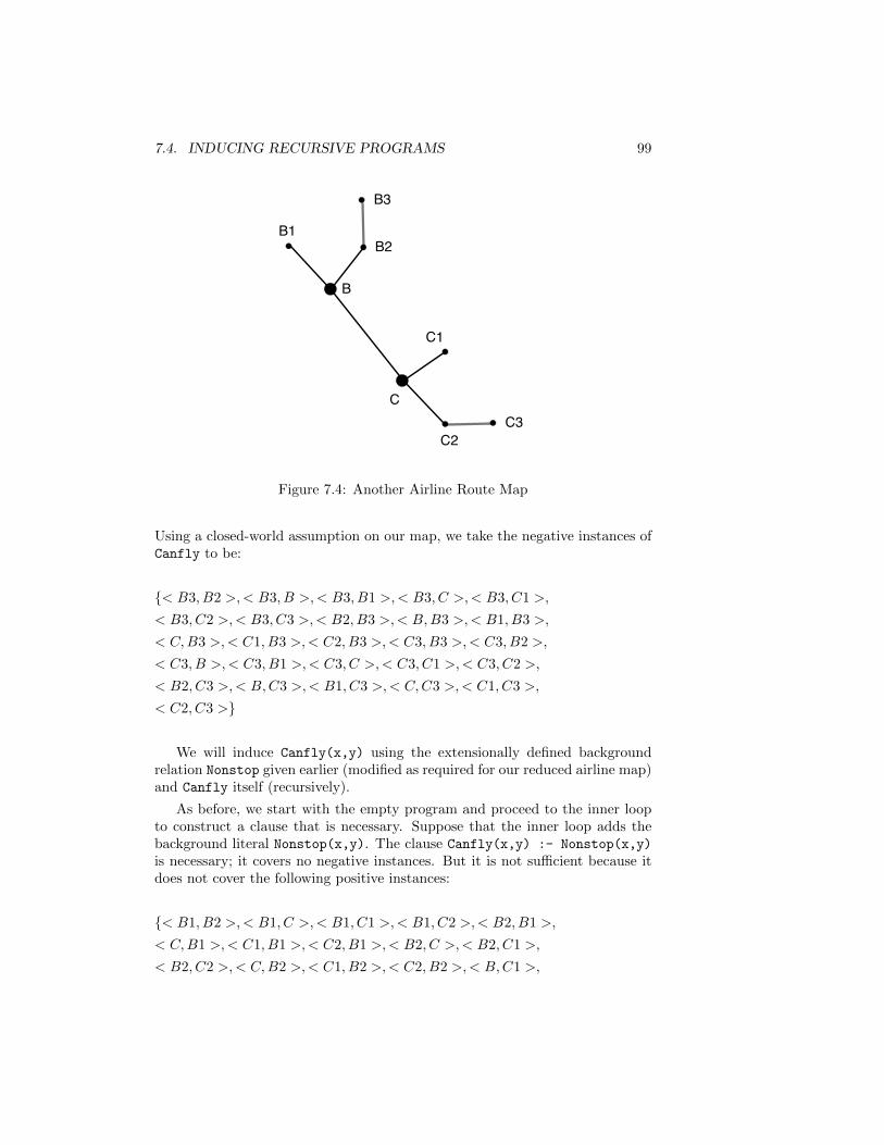
7.4. INDUCING RECURSIVE PROGRAMS 99
B
C
C1
C2
B1B2
B3
C3
Figure 7.4: Another Airline Route Map
Using a closed-world assumption on our map, we take the negative instances ofCanfly to be:
< B3, B2 >,< B3, B >,< B3, B1 >,< B3, C >,< B3, C1 >,
< B3, C2 >,< B3, C3 >,< B2, B3 >,< B,B3 >,< B1, B3 >,
< C,B3 >,< C1, B3 >,< C2, B3 >,< C3, B3 >,< C3, B2 >,
< C3, B >,< C3, B1 >,< C3, C >,< C3, C1 >,< C3, C2 >,
< B2, C3 >,< B,C3 >,< B1, C3 >,< C,C3 >,< C1, C3 >,
< C2, C3 >
We will induce Canfly(x,y) using the extensionally defined backgroundrelation Nonstop given earlier (modified as required for our reduced airline map)and Canfly itself (recursively).
As before, we start with the empty program and proceed to the inner loopto construct a clause that is necessary. Suppose that the inner loop adds thebackground literal Nonstop(x,y). The clause Canfly(x,y) :- Nonstop(x,y)
is necessary; it covers no negative instances. But it is not sufficient because itdoes not cover the following positive instances:
< B1, B2 >,< B1, C >,< B1, C1 >,< B1, C2 >,< B2, B1 >,
< C,B1 >,< C1, B1 >,< C2, B1 >,< B2, C >,< B2, C1 >,
< B2, C2 >,< C,B2 >,< C1, B2 >,< C2, B2 >,< B,C1 >,
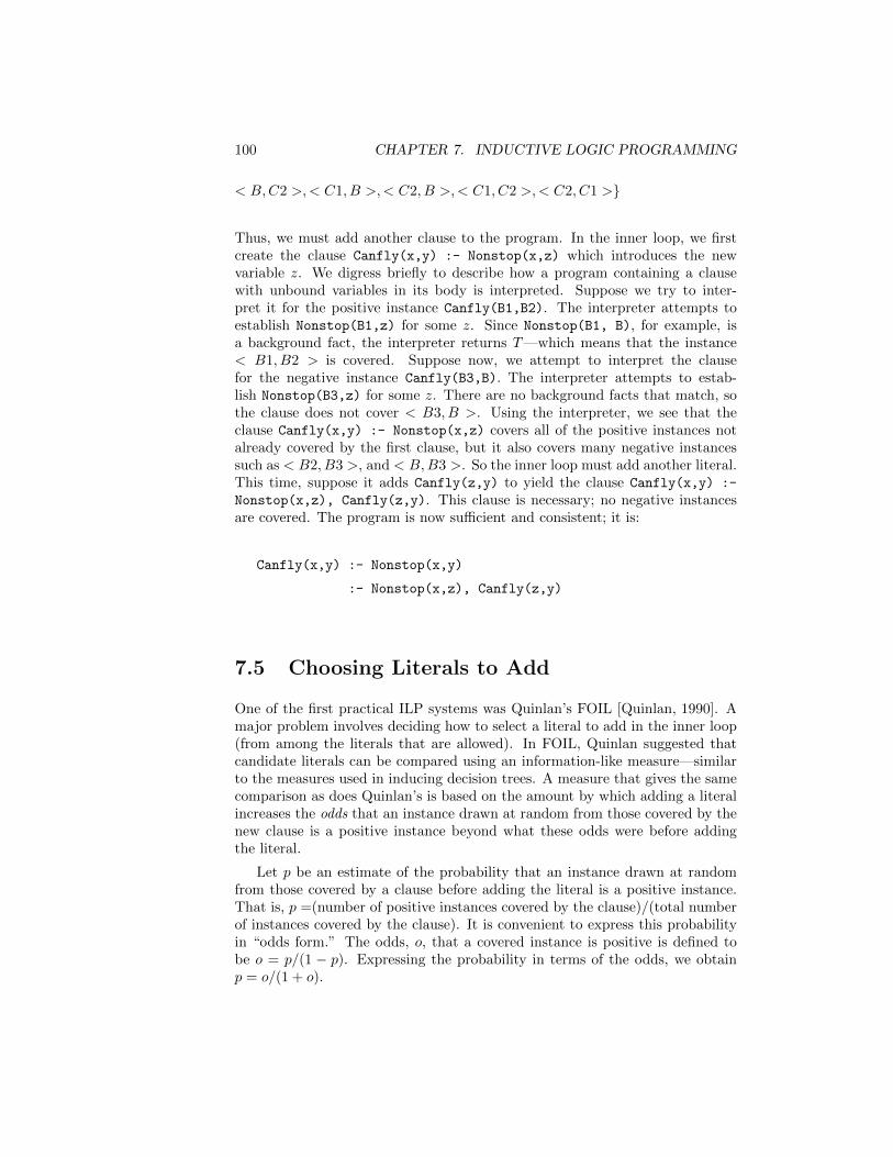
100 CHAPTER 7. INDUCTIVE LOGIC PROGRAMMING
< B,C2 >,< C1, B >,< C2, B >,< C1, C2 >,< C2, C1 >
Thus, we must add another clause to the program. In the inner loop, we firstcreate the clause Canfly(x,y) :- Nonstop(x,z) which introduces the newvariable z. We digress briefly to describe how a program containing a clausewith unbound variables in its body is interpreted. Suppose we try to inter-pret it for the positive instance Canfly(B1,B2). The interpreter attempts toestablish Nonstop(B1,z) for some z. Since Nonstop(B1, B), for example, isa background fact, the interpreter returns T—which means that the instance< B1, B2 > is covered. Suppose now, we attempt to interpret the clausefor the negative instance Canfly(B3,B). The interpreter attempts to estab-lish Nonstop(B3,z) for some z. There are no background facts that match, sothe clause does not cover < B3, B >. Using the interpreter, we see that theclause Canfly(x,y) :- Nonstop(x,z) covers all of the positive instances notalready covered by the first clause, but it also covers many negative instancessuch as < B2, B3 >, and < B,B3 >. So the inner loop must add another literal.This time, suppose it adds Canfly(z,y) to yield the clause Canfly(x,y) :-
Nonstop(x,z), Canfly(z,y). This clause is necessary; no negative instancesare covered. The program is now sufficient and consistent; it is:
Canfly(x,y) :- Nonstop(x,y)
:- Nonstop(x,z), Canfly(z,y)
7.5 Choosing Literals to Add
One of the first practical ILP systems was Quinlan’s FOIL [Quinlan, 1990]. Amajor problem involves deciding how to select a literal to add in the inner loop(from among the literals that are allowed). In FOIL, Quinlan suggested thatcandidate literals can be compared using an information-like measure—similarto the measures used in inducing decision trees. A measure that gives the samecomparison as does Quinlan’s is based on the amount by which adding a literalincreases the odds that an instance drawn at random from those covered by thenew clause is a positive instance beyond what these odds were before addingthe literal.
Let p be an estimate of the probability that an instance drawn at randomfrom those covered by a clause before adding the literal is a positive instance.That is, p =(number of positive instances covered by the clause)/(total numberof instances covered by the clause). It is convenient to express this probabilityin “odds form.” The odds, o, that a covered instance is positive is defined tobe o = p/(1 − p). Expressing the probability in terms of the odds, we obtainp = o/(1 + o).
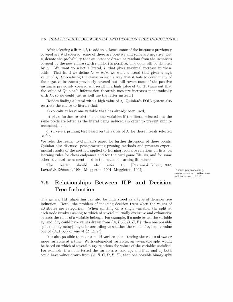
7.6. RELATIONSHIPS BETWEEN ILP ANDDECISION TREE INDUCTION101
After selecting a literal, l, to add to a clause, some of the instances previouslycovered are still covered; some of these are positive and some are negative. Letpl denote the probability that an instance drawn at random from the instancescovered by the new clause (with l added) is positive. The odds will be denotedby ol. We want to select a literal, l, that gives maximal increase in theseodds. That is, if we define λl = ol/o, we want a literal that gives a highvalue of λl. Specializing the clause in such a way that it fails to cover many ofthe negative instances previously covered but still covers most of the positiveinstances previously covered will result in a high value of λl. (It turns out thatthe value of Quinlan’s information theoretic measure increases monotonicallywith λl, so we could just as well use the latter instead.)
Besides finding a literal with a high value of λl, Quinlan’s FOIL system alsorestricts the choice to literals that:
a) contain at least one variable that has already been used,
b) place further restrictions on the variables if the literal selected has thesame predicate letter as the literal being induced (in order to prevent infiniterecursion), and
c) survive a pruning test based on the values of λl for those literals selectedso far.
We refer the reader to Quinlan’s paper for further discussion of these points.Quinlan also discusses post-processing pruning methods and presents experi-mental results of the method applied to learning recursive relations on lists, onlearning rules for chess endgames and for the card game Eleusis, and for someother standard tasks mentioned in the machine learning literature.
The reader should also refer to [Pazzani & Kibler, 1992,Lavrac & Dzeroski, 1994, Muggleton, 1991, Muggleton, 1992]. Discuss preprocessing,
postprocessing, bottom-upmethods, and LINUS.
7.6 Relationships Between ILP and DecisionTree Induction
The generic ILP algorithm can also be understood as a type of decision treeinduction. Recall the problem of inducing decision trees when the values ofattributes are categorical. When splitting on a single variable, the split ateach node involves asking to which of several mutually exclusive and exhaustivesubsets the value of a variable belongs. For example, if a node tested the variablexi, and if xi could have values drawn from A,B,C,D,E, F, then one possiblesplit (among many) might be according to whether the value of xi had as valueone of A,B,C or one of D,E, F.
It is also possible to make a multi-variate split—testing the values of two ormore variables at a time. With categorical variables, an n-variable split wouldbe based on which of several n-ary relations the values of the variables satisfied.For example, if a node tested the variables xi and xj , and if xi and xj bothcould have values drawn from A,B,C,D,E, F, then one possible binary split
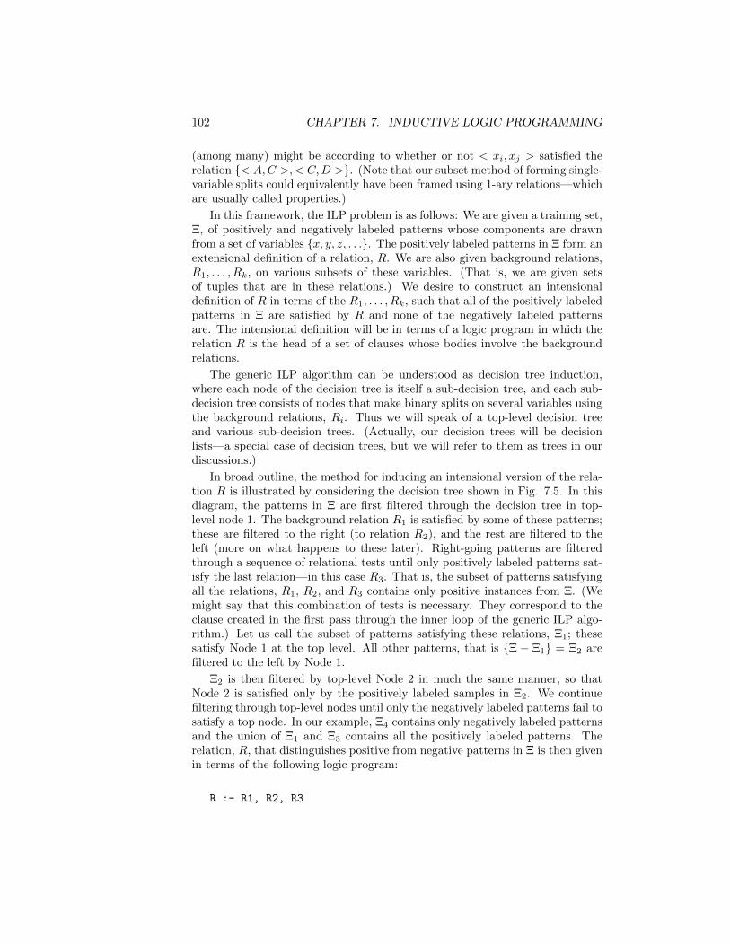
102 CHAPTER 7. INDUCTIVE LOGIC PROGRAMMING
(among many) might be according to whether or not < xi, xj > satisfied therelation < A,C >,< C,D >. (Note that our subset method of forming single-variable splits could equivalently have been framed using 1-ary relations—whichare usually called properties.)
In this framework, the ILP problem is as follows: We are given a training set,Ξ, of positively and negatively labeled patterns whose components are drawnfrom a set of variables x, y, z, . . .. The positively labeled patterns in Ξ form anextensional definition of a relation, R. We are also given background relations,R1, . . . , Rk, on various subsets of these variables. (That is, we are given setsof tuples that are in these relations.) We desire to construct an intensionaldefinition of R in terms of the R1, . . . , Rk, such that all of the positively labeledpatterns in Ξ are satisfied by R and none of the negatively labeled patternsare. The intensional definition will be in terms of a logic program in which therelation R is the head of a set of clauses whose bodies involve the backgroundrelations.
The generic ILP algorithm can be understood as decision tree induction,where each node of the decision tree is itself a sub-decision tree, and each sub-decision tree consists of nodes that make binary splits on several variables usingthe background relations, Ri. Thus we will speak of a top-level decision treeand various sub-decision trees. (Actually, our decision trees will be decisionlists—a special case of decision trees, but we will refer to them as trees in ourdiscussions.)
In broad outline, the method for inducing an intensional version of the rela-tion R is illustrated by considering the decision tree shown in Fig. 7.5. In thisdiagram, the patterns in Ξ are first filtered through the decision tree in top-level node 1. The background relation R1 is satisfied by some of these patterns;these are filtered to the right (to relation R2), and the rest are filtered to theleft (more on what happens to these later). Right-going patterns are filteredthrough a sequence of relational tests until only positively labeled patterns sat-isfy the last relation—in this case R3. That is, the subset of patterns satisfyingall the relations, R1, R2, and R3 contains only positive instances from Ξ. (Wemight say that this combination of tests is necessary. They correspond to theclause created in the first pass through the inner loop of the generic ILP algo-rithm.) Let us call the subset of patterns satisfying these relations, Ξ1; thesesatisfy Node 1 at the top level. All other patterns, that is Ξ − Ξ1 = Ξ2 arefiltered to the left by Node 1.
Ξ2 is then filtered by top-level Node 2 in much the same manner, so thatNode 2 is satisfied only by the positively labeled samples in Ξ2. We continuefiltering through top-level nodes until only the negatively labeled patterns fail tosatisfy a top node. In our example, Ξ4 contains only negatively labeled patternsand the union of Ξ1 and Ξ3 contains all the positively labeled patterns. Therelation, R, that distinguishes positive from negative patterns in Ξ is then givenin terms of the following logic program:
R :- R1, R2, R3
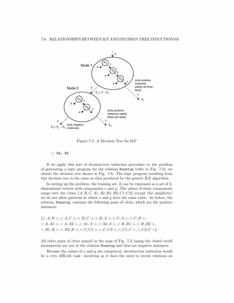
7.6. RELATIONSHIPS BETWEEN ILP ANDDECISION TREE INDUCTION103
R1
R2
R3
T
T
T
F
F
F
T
F
R4
R5
T
T
F
F
TF
1
2 = 1
34= 2 3
Node 1
Node 2
(only positiveinstancessatisfy all threetests)
(only positivelinstances satisfythese two tests)
(only negativeinstances)
Figure 7.5: A Decision Tree for ILP
:- R4, R5
If we apply this sort of decision-tree induction procedure to the problemof generating a logic program for the relation Nonstop (refer to Fig. 7.3), weobtain the decision tree shown in Fig. 7.6. The logic program resulting fromthis decision tree is the same as that produced by the generic ILP algorithm.
In setting up the problem, the training set, Ξ can be expressed as a set of 2-dimensional vectors with components x and y. The values of these componentsrange over the cities A,B,C,A1, A2, B1, B2, C1, C2 except (for simplicity)we do not allow patterns in which x and y have the same value. As before, therelation, Nonstop, contains the following pairs of cities, which are the positiveinstances:
< A,B >,< A,C >,< B,C >,< B,A >,< C,A >,< C,B >,
< A,A1 >,< A,A2 >,< A1, A >,< A2, A >,< B,B1 >,< B,B2 >,
< B1, B >,< B2, B >,< C,C1 >,< C,C2 >,< C1, C >,< C2, C >
All other pairs of cities named in the map of Fig. 7.3 (using the closed worldassumption) are not in the relation Nonstop and thus are negative instances.
Because the values of x and y are categorical, decision-tree induction wouldbe a very difficult task—involving as it does the need to invent relations on

104 CHAPTER 7. INDUCTIVE LOGIC PROGRAMMING
x and y to be used as tests. But with the background relations, Ri (in thiscase Hub and Satellite), the problem is made much easier. We select theserelations in the same way that we select literals; from among the available tests,we make a selection based on which leads to the largest value of λRi .
7.7 Bibliographical and Historical RemarksTo be added.
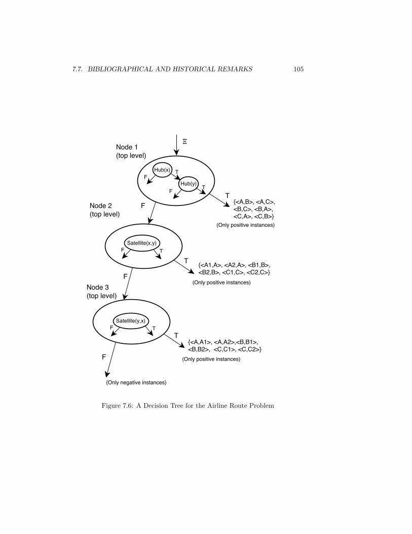
7.7. BIBLIOGRAPHICAL AND HISTORICAL REMARKS 105
Hub(x) TF
Node 1(top level)
<A,B>, <A,C>,<B,C>, <B,A>,<C,A>, <C,B>
Hub(y) TT
FNode 2(top level)
Satellite(x,y)F T
T <A1,A>, <A2,A>, <B1,B>,<B2,B>, <C1,C>, <C2,C>
F
<A,A1>, <A,A2>,<B,B1>,<B,B2>, <C,C1>, <C,C2>
Satellite(y,x)F
F
T
Node 3(top level)
T
Only negative instances
(Only positive instances)
(Only positive instances)
(Only positive instances)
F
Figure 7.6: A Decision Tree for the Airline Route Problem

106 CHAPTER 7. INDUCTIVE LOGIC PROGRAMMING
Chapter 8
Computational LearningTheory
In chapter one we posed the problem of guessing a function given a set ofsample inputs and their values. We gave some intuitive arguments to supportthe claim that after seeing only a small fraction of the possible inputs (andtheir values) that we could guess almost correctly the values of most subsequentinputs—if we knew that the function we were trying to guess belonged to anappropriately restricted subset of functions. That is, a given training set ofsample patterns might be adequate to allow us to select a function, consistentwith the labeled samples, from among a restricted set of hypotheses such thatwith high probability the function we select will be approximately correct (smallprobability of error) on subsequent samples drawn at random according to thesame distribution from which the labeled samples were drawn. This insightled to the theory of probably approximately correct (PAC) learning—initiallydeveloped by Leslie Valiant [Valiant, 1984]. We present here a brief descriptionof the theory for the case of Boolean functions. [Dietterich, 1990, Haussler, 1988,Haussler, 1990] give nice surveys of the important results. Other overviews?
8.1 Notation and Assumptions for PAC Learn-ing Theory
We assume a training set Ξ of n-dimensional vectors, Xi, i = 1, . . . ,m, eachlabeled (by 1 or 0) according to a target function, f , which is unknown tothe learner. The probability of any given vector X being in Ξ, or later beingpresented to the learner, is P (X). The probability distribution, P , can bearbitrary. (In the literature of PAC learning theory, the target function is usuallycalled the target concept and is denoted by c, but to be consistent with ourprevious notation we will continue to denote it by f .) Our problem is to guess
107
108 CHAPTER 8. COMPUTATIONAL LEARNING THEORY
a function, h(X), based on the labeled samples in Ξ. In PAC theory such aguessed function is called the hypothesis. We assume that the target functionis some element of a set of functions, C. We also assume that the hypothesis,h, is an element of a set, H, of hypotheses, which includes the set, C, of targetfunctions. H is called the hypothesis space.
In general, h won’t be identical to f , but we can strive to have the value ofh(X) = the value of f(X) for most X’s. That is, we want h to be approximatelycorrect. To quantify this notion, we define the error of h, εh, as the probabilitythat an X drawn randomly according to P will be misclassified:
εh =∑
[X:h(X) 6=f(X)]
P (X)
Boldface symbols need to besmaller when they are subscripts inmath environments.
We say that h is approximately (except for ε ) correct if εh ≤ ε, where ε is theaccuracy parameter.
Suppose we are able to find an h that classifies all m randomly drawn trainingsamples correctly; that is, h is consistent with this randomly selected trainingset, Ξ. If m is large enough, will such an h be approximately correct (andfor what value of ε)? On some training occasions, using m randomly drawntraining samples, such an h might turn out to be approximately correct (for agiven value of ε), and on others it might not. We say that h is probably (exceptfor δ) approximately correct (PAC) if the probability that it is approximatelycorrect is greater than 1−δ, where δ is the confidence parameter. We shall showthat if m is greater than some bound whose value depends on ε and δ, such anh is guaranteed to be probably approximately correct.
In general, we say that a learning algorithm PAC-learns functions from C interms of H iff for every function fε C, it outputs a hypothesis hε H, such thatwith probability at least (1 − δ), εh ≤ ε. Such a hypothesis is called probably(except for δ) approximately (except for ε) correct.
We want learning algorithms that are tractable, so we want an algorithmthat PAC-learns functions in polynomial time. This can only be done for certainclasses of functions. If there are a finite number of hypotheses in a hypothesisset (as there are for many of the hypothesis sets we have considered), we couldalways produce a consistent hypothesis from this set by testing all of themagainst the training data. But if there are an exponential number of hypotheses,that would take exponential time. We seek training methods that produceconsistent hypotheses in less time. The time complexities for various hypothesissets have been determined, and these are summarized in a table to be presentedlater.
A class, C, is polynomially PAC learnable in terms of H provided there existsa polynomial-time learning algorithm (polynomial in the number of samplesneeded, m, in the dimension, n, in 1/ε, and in 1/δ) that PAC-learns functionsin C in terms of H.
Initial work on PAC assumed H = C, but it was later shown that some func-tions cannot be polynomially PAC-learned under such an assumption (assuming
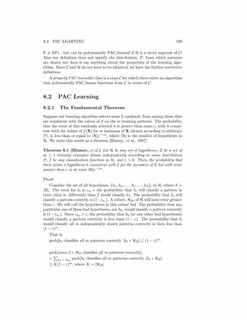
8.2. PAC LEARNING 109
P 6= NP)—but can be polynomially PAC-learned if H is a strict superset of C!Also our definition does not specify the distribution, P , from which patternsare drawn nor does it say anything about the properties of the learning algo-rithm. Since C and H do not have to be identical, we have the further restrictivedefinition:
A properly PAC-learnable class is a class C for which there exists an algorithmthat polynomially PAC-learns functions from C in terms of C.
8.2 PAC Learning
8.2.1 The Fundamental Theorem
Suppose our learning algorithm selects some h randomly from among those thatare consistent with the values of f on the m training patterns. The probabilitythat the error of this randomly selected h is greater than some ε, with h consis-tent with the values of f(X) for m instances of X (drawn according to arbitraryP ), is less than or equal to |H|e−εm, where |H| is the number of hypotheses inH. We state this result as a theorem [Blumer, et al., 1987]:
Theorem 8.1 (Blumer, et al.) Let H be any set of hypotheses, Ξ be a set ofm ≥ 1 training examples drawn independently according to some distributionP , f be any classification function in H, and ε > 0. Then, the probability thatthere exists a hypothesis h consistent with f for the members of Ξ but with errorgreater than ε is at most |H|e−εm.
Proof:
Consider the set of all hypotheses, h1, h2, . . . , hi, . . . , hS, in H, where S =|H|. The error for hi is εhi= the probability that hi will classify a pattern inerror (that is, differently than f would classify it). The probability that hi willclassify a pattern correctly is (1−εhi). A subset, HB , ofH will have error greaterthan ε. We will call the hypotheses in this subset bad. The probability that anyparticular one of these bad hypotheses, say hb, would classify a pattern correctlyis (1−εhb). Since εhb > ε, the probability that hb (or any other bad hypothesis)would classify a pattern correctly is less than (1 − ε). The probability that itwould classify all m independently drawn patterns correctly is then less than(1− ε)m.
That is,
prob[hb classifies all m patterns correctly |hb ε HB ] ≤ (1− ε)m.
prob[some h ε HB classifies all m patterns correctly]
=∑hb ε HB prob[hb classifies all m patterns correctly |hb ε HB ]
≤ K(1− ε)m, where K = |HB |.
110 CHAPTER 8. COMPUTATIONAL LEARNING THEORY
That is,
prob[there is a bad hypothesis that classifies all m patterns correctly]
≤ K(1− ε)m.
Since K ≤ |H| and (1− ε)m ≤ e−εm, we have:
prob[there is a bad hypothesis that classifies all m patterns correctly]
= prob[there is a hypothesis with error > ε and that classifies all m patternscorrectly] ≤ |H|e−εm.
QED
A corollary of this theorem is:
Corollary 8.2 Given m ≥ (1/ε)(ln |H|+ ln(1/δ)) independent samples, theprobability that there exists a hypothesis in H that is consistent with f on thesesamples and has error greater than ε is at most δ.
Proof: We are to find a bound on m that guarantees that
prob[there is a hypothesis with error > ε and that classifies all m patternscorrectly] ≤ δ. Thus, using the result of the theorem, we must show that|H|e−εm ≤ δ. Taking the natural logarithm of both sides yields:
ln |H| − εm ≤ ln δ
or
m ≥ (1/ε)(ln |H|+ ln(1/δ))
QED
This corollary is important for two reasons. First it clearly states that wecan select any hypothesis consistent with the m samples and be assured thatwith probability (1 − δ) its error will be less than ε. Also, it shows that inorder for m to increase no more than polynomially with n, |H| can be no larger
than 2O(nk). No class larger than that can be guaranteed to be properly PAClearnable.
Here is a possible point of confusion: The bound given in the corollary isan upper bound on the value of m needed to guarantee polynomial probably ap-proximately correct learning. Values of m greater than that bound are sufficient(but might not be necessary). We will present a lower (necessary) bound laterin the chapter.
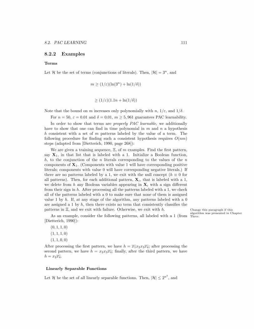
8.2. PAC LEARNING 111
8.2.2 Examples
Terms
Let H be the set of terms (conjunctions of literals). Then, |H| = 3n, and
m ≥ (1/ε)(ln(3n) + ln(1/δ))
≥ (1/ε)(1.1n+ ln(1/δ))
Note that the bound on m increases only polynomially with n, 1/ε, and 1/δ.
For n = 50, ε = 0.01 and δ = 0.01, m ≥ 5, 961 guarantees PAC learnability.
In order to show that terms are properly PAC learnable, we additionallyhave to show that one can find in time polynomial in m and n a hypothesish consistent with a set of m patterns labeled by the value of a term. Thefollowing procedure for finding such a consistent hypothesis requires O(nm)steps (adapted from [Dietterich, 1990, page 268]):
We are given a training sequence, Ξ, of m examples. Find the first pattern,say X1, in that list that is labeled with a 1. Initialize a Boolean function,h, to the conjunction of the n literals corresponding to the values of the ncomponents of X1. (Components with value 1 will have corresponding positiveliterals; components with value 0 will have corresponding negative literals.) Ifthere are no patterns labeled by a 1, we exit with the null concept (h ≡ 0 forall patterns). Then, for each additional pattern, Xi, that is labeled with a 1,we delete from h any Boolean variables appearing in Xi with a sign differentfrom their sign in h. After processing all the patterns labeled with a 1, we checkall of the patterns labeled with a 0 to make sure that none of them is assignedvalue 1 by h. If, at any stage of the algorithm, any patterns labeled with a 0are assigned a 1 by h, then there exists no term that consistently classifies thepatterns in Ξ, and we exit with failure. Otherwise, we exit with h. Change this paragraph if this
algorithm was presented in ChapterThree.As an example, consider the following patterns, all labeled with a 1 (from
[Dietterich, 1990]):
(0, 1, 1, 0)
(1, 1, 1, 0)
(1, 1, 0, 0)
After processing the first pattern, we have h = x1x2x3x4; after processing thesecond pattern, we have h = x2x3x4; finally, after the third pattern, we haveh = x2x4.
Linearly Separable Functions
Let H be the set of all linearly separable functions. Then, |H| ≤ 2n2
, and
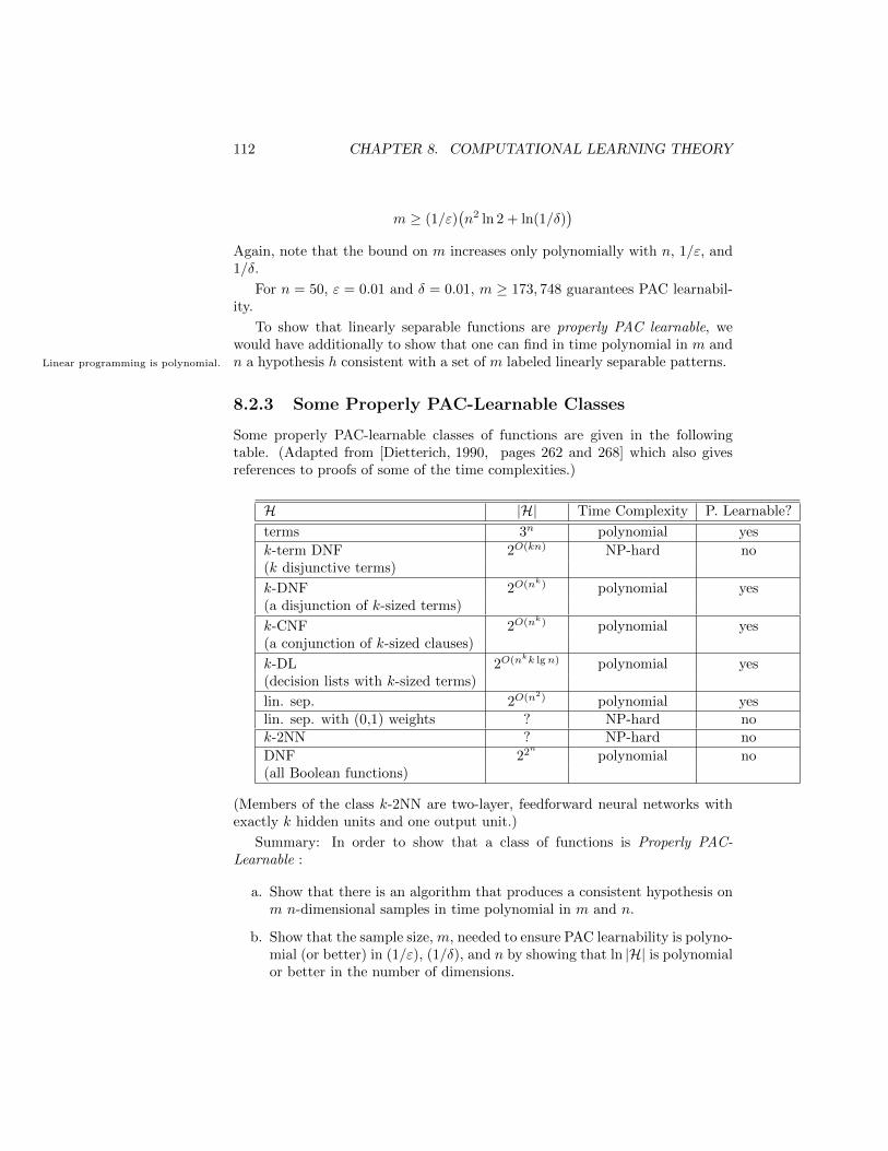
112 CHAPTER 8. COMPUTATIONAL LEARNING THEORY
m ≥ (1/ε)(n2 ln 2 + ln(1/δ)
)Again, note that the bound on m increases only polynomially with n, 1/ε, and1/δ.
For n = 50, ε = 0.01 and δ = 0.01, m ≥ 173, 748 guarantees PAC learnabil-ity.
To show that linearly separable functions are properly PAC learnable, wewould have additionally to show that one can find in time polynomial in m andn a hypothesis h consistent with a set of m labeled linearly separable patterns.Linear programming is polynomial.
8.2.3 Some Properly PAC-Learnable Classes
Some properly PAC-learnable classes of functions are given in the followingtable. (Adapted from [Dietterich, 1990, pages 262 and 268] which also givesreferences to proofs of some of the time complexities.)
H |H| Time Complexity P. Learnable?
terms 3n polynomial yes
k-term DNF 2O(kn) NP-hard no(k disjunctive terms)
k-DNF 2O(nk) polynomial yes(a disjunction of k-sized terms)
k-CNF 2O(nk) polynomial yes(a conjunction of k-sized clauses)
k-DL 2O(nkk lgn) polynomial yes(decision lists with k-sized terms)
lin. sep. 2O(n2) polynomial yeslin. sep. with (0,1) weights ? NP-hard nok-2NN ? NP-hard no
DNF 22n polynomial no(all Boolean functions)
(Members of the class k-2NN are two-layer, feedforward neural networks withexactly k hidden units and one output unit.)
Summary: In order to show that a class of functions is Properly PAC-Learnable :
a. Show that there is an algorithm that produces a consistent hypothesis onm n-dimensional samples in time polynomial in m and n.
b. Show that the sample size, m, needed to ensure PAC learnability is polyno-mial (or better) in (1/ε), (1/δ), and n by showing that ln |H| is polynomialor better in the number of dimensions.
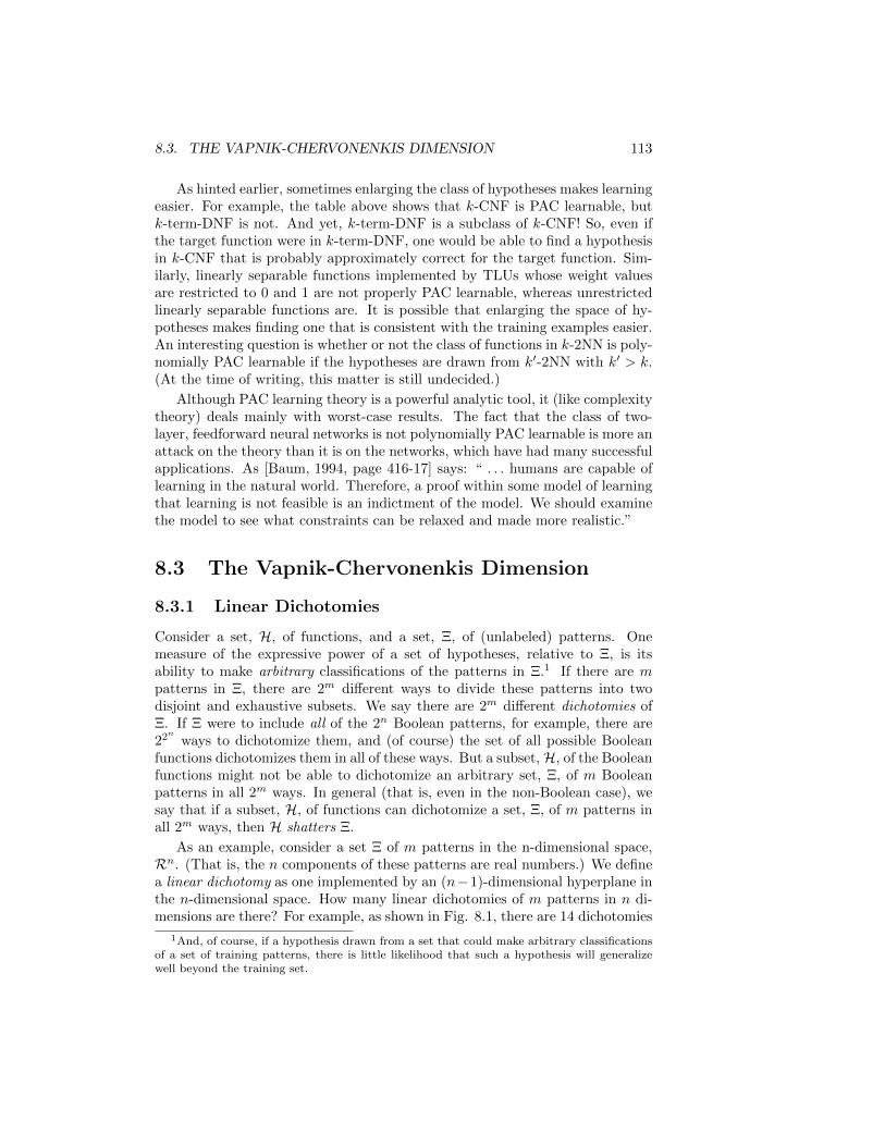
8.3. THE VAPNIK-CHERVONENKIS DIMENSION 113
As hinted earlier, sometimes enlarging the class of hypotheses makes learningeasier. For example, the table above shows that k-CNF is PAC learnable, butk-term-DNF is not. And yet, k-term-DNF is a subclass of k-CNF! So, even ifthe target function were in k-term-DNF, one would be able to find a hypothesisin k-CNF that is probably approximately correct for the target function. Sim-ilarly, linearly separable functions implemented by TLUs whose weight valuesare restricted to 0 and 1 are not properly PAC learnable, whereas unrestrictedlinearly separable functions are. It is possible that enlarging the space of hy-potheses makes finding one that is consistent with the training examples easier.An interesting question is whether or not the class of functions in k-2NN is poly-nomially PAC learnable if the hypotheses are drawn from k′-2NN with k′ > k.(At the time of writing, this matter is still undecided.)
Although PAC learning theory is a powerful analytic tool, it (like complexitytheory) deals mainly with worst-case results. The fact that the class of two-layer, feedforward neural networks is not polynomially PAC learnable is more anattack on the theory than it is on the networks, which have had many successfulapplications. As [Baum, 1994, page 416-17] says: “ . . . humans are capable oflearning in the natural world. Therefore, a proof within some model of learningthat learning is not feasible is an indictment of the model. We should examinethe model to see what constraints can be relaxed and made more realistic.”
8.3 The Vapnik-Chervonenkis Dimension
8.3.1 Linear Dichotomies
Consider a set, H, of functions, and a set, Ξ, of (unlabeled) patterns. Onemeasure of the expressive power of a set of hypotheses, relative to Ξ, is itsability to make arbitrary classifications of the patterns in Ξ.1 If there are mpatterns in Ξ, there are 2m different ways to divide these patterns into twodisjoint and exhaustive subsets. We say there are 2m different dichotomies ofΞ. If Ξ were to include all of the 2n Boolean patterns, for example, there are22n ways to dichotomize them, and (of course) the set of all possible Booleanfunctions dichotomizes them in all of these ways. But a subset,H, of the Booleanfunctions might not be able to dichotomize an arbitrary set, Ξ, of m Booleanpatterns in all 2m ways. In general (that is, even in the non-Boolean case), wesay that if a subset, H, of functions can dichotomize a set, Ξ, of m patterns inall 2m ways, then H shatters Ξ.
As an example, consider a set Ξ of m patterns in the n-dimensional space,Rn. (That is, the n components of these patterns are real numbers.) We definea linear dichotomy as one implemented by an (n−1)-dimensional hyperplane inthe n-dimensional space. How many linear dichotomies of m patterns in n di-mensions are there? For example, as shown in Fig. 8.1, there are 14 dichotomies
1And, of course, if a hypothesis drawn from a set that could make arbitrary classificationsof a set of training patterns, there is little likelihood that such a hypothesis will generalizewell beyond the training set.
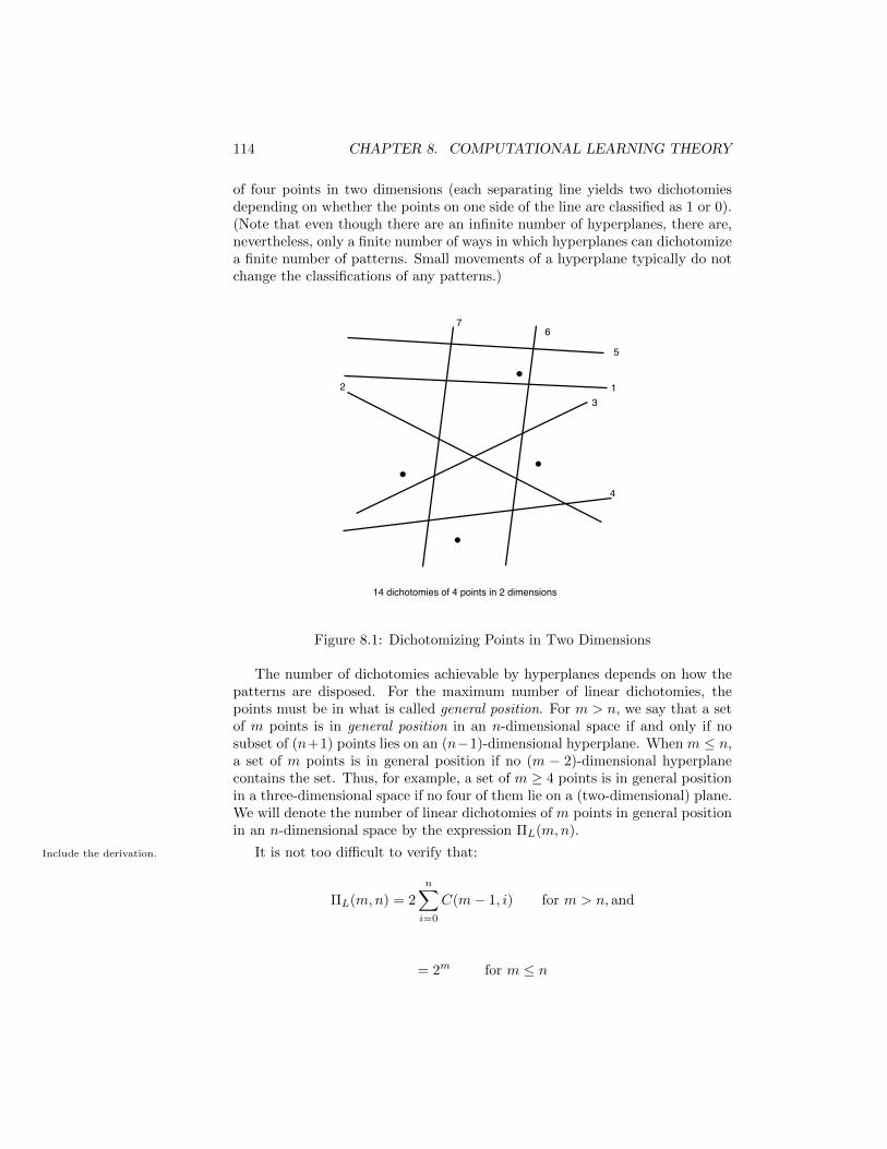
114 CHAPTER 8. COMPUTATIONAL LEARNING THEORY
of four points in two dimensions (each separating line yields two dichotomiesdepending on whether the points on one side of the line are classified as 1 or 0).(Note that even though there are an infinite number of hyperplanes, there are,nevertheless, only a finite number of ways in which hyperplanes can dichotomizea finite number of patterns. Small movements of a hyperplane typically do notchange the classifications of any patterns.)
123
4
14 dichotomies of 4 points in 2 dimensions
5
67
Figure 8.1: Dichotomizing Points in Two Dimensions
The number of dichotomies achievable by hyperplanes depends on how thepatterns are disposed. For the maximum number of linear dichotomies, thepoints must be in what is called general position. For m > n, we say that a setof m points is in general position in an n-dimensional space if and only if nosubset of (n+1) points lies on an (n−1)-dimensional hyperplane. When m ≤ n,a set of m points is in general position if no (m − 2)-dimensional hyperplanecontains the set. Thus, for example, a set of m ≥ 4 points is in general positionin a three-dimensional space if no four of them lie on a (two-dimensional) plane.We will denote the number of linear dichotomies of m points in general positionin an n-dimensional space by the expression ΠL(m,n).
It is not too difficult to verify that:Include the derivation.
ΠL(m,n) = 2
n∑i=0
C(m− 1, i) for m > n, and
= 2m for m ≤ n
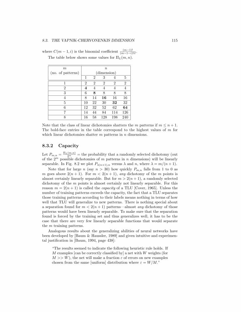
8.3. THE VAPNIK-CHERVONENKIS DIMENSION 115
where C(m− 1, i) is the binomial coefficient (m−1)!(m−1−i)!i! .
The table below shows some values for ΠL(m,n).
m n(no. of patterns) (dimension)
1 2 3 4 5
1 2 2 2 2 22 4 4 4 4 43 6 8 8 8 84 8 14 16 16 165 10 22 30 32 326 12 32 52 62 647 14 44 84 114 1268 16 58 128 198 240
Note that the class of linear dichotomies shatters the m patterns if m ≤ n+ 1.The bold-face entries in the table correspond to the highest values of m forwhich linear dichotomies shatter m patterns in n dimensions.
8.3.2 Capacity
Let Pm,n = ΠL(m,n)2m = the probability that a randomly selected dichotomy (out
of the 2m possible dichotomies of m patterns in n dimensions) will be linearlyseparable. In Fig. 8.2 we plot Pλ(n+1),n versus λ and n, where λ = m/(n+ 1).
Note that for large n (say n > 30) how quickly Pm,n falls from 1 to 0 asm goes above 2(n + 1). For m < 2(n + 1), any dichotomy of the m points isalmost certainly linearly separable. But for m > 2(n+ 1), a randomly selecteddichotomy of the m points is almost certainly not linearly separable. For thisreason m = 2(n + 1) is called the capacity of a TLU [Cover, 1965]. Unless thenumber of training patterns exceeds the capacity, the fact that a TLU separatesthose training patterns according to their labels means nothing in terms of howwell that TLU will generalize to new patterns. There is nothing special abouta separation found for m < 2(n + 1) patterns—almost any dichotomy of thosepatterns would have been linearly separable. To make sure that the separationfound is forced by the training set and thus generalizes well, it has to be thecase that there are very few linearly separable functions that would separatethe m training patterns.
Analogous results about the generalizing abilities of neural networks havebeen developed by [Baum & Haussler, 1989] and given intuitive and experimen-tal justification in [Baum, 1994, page 438]:
“The results seemed to indicate the following heuristic rule holds. IfM examples [can be correctly classified by] a net with W weights (forM >> W ), the net will make a fraction ε of errors on new exampleschosen from the same [uniform] distribution where ε = W/M .”
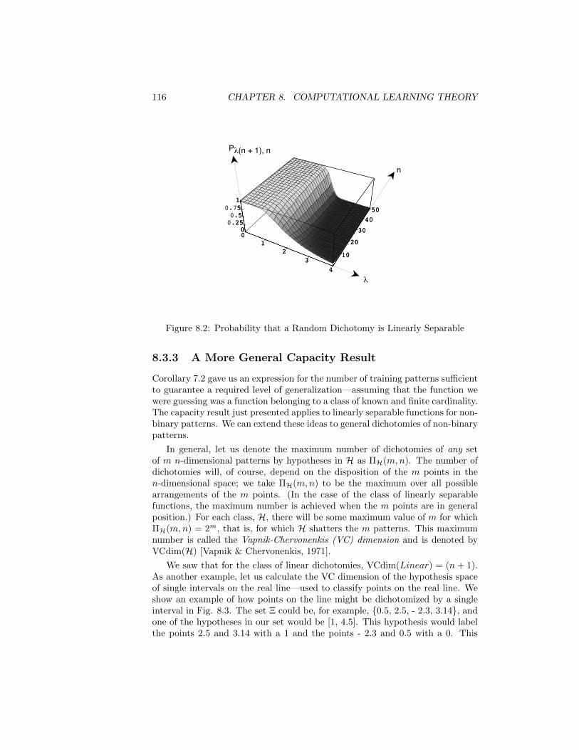
116 CHAPTER 8. COMPUTATIONAL LEARNING THEORY
01
23
4
10
20
30
4050
00.250.5
0.751
01
23
4
10
20
30
4050
025.5751
P (n + 1), n
n
Figure 8.2: Probability that a Random Dichotomy is Linearly Separable
8.3.3 A More General Capacity Result
Corollary 7.2 gave us an expression for the number of training patterns sufficientto guarantee a required level of generalization—assuming that the function wewere guessing was a function belonging to a class of known and finite cardinality.The capacity result just presented applies to linearly separable functions for non-binary patterns. We can extend these ideas to general dichotomies of non-binarypatterns.
In general, let us denote the maximum number of dichotomies of any setof m n-dimensional patterns by hypotheses in H as ΠH(m,n). The number ofdichotomies will, of course, depend on the disposition of the m points in then-dimensional space; we take ΠH(m,n) to be the maximum over all possiblearrangements of the m points. (In the case of the class of linearly separablefunctions, the maximum number is achieved when the m points are in generalposition.) For each class, H, there will be some maximum value of m for whichΠH(m,n) = 2m, that is, for which H shatters the m patterns. This maximumnumber is called the Vapnik-Chervonenkis (VC) dimension and is denoted byVCdim(H) [Vapnik & Chervonenkis, 1971].
We saw that for the class of linear dichotomies, VCdim(Linear) = (n + 1).As another example, let us calculate the VC dimension of the hypothesis spaceof single intervals on the real line—used to classify points on the real line. Weshow an example of how points on the line might be dichotomized by a singleinterval in Fig. 8.3. The set Ξ could be, for example, 0.5, 2.5, - 2.3, 3.14, andone of the hypotheses in our set would be [1, 4.5]. This hypothesis would labelthe points 2.5 and 3.14 with a 1 and the points - 2.3 and 0.5 with a 0. This
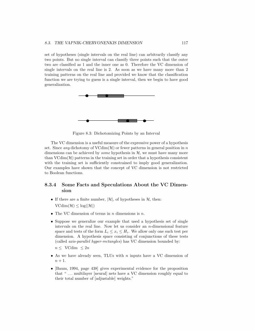
8.3. THE VAPNIK-CHERVONENKIS DIMENSION 117
set of hypotheses (single intervals on the real line) can arbitrarily classify anytwo points. But no single interval can classify three points such that the outertwo are classified as 1 and the inner one as 0. Therefore the VC dimension ofsingle intervals on the real line is 2. As soon as we have many more than 2training patterns on the real line and provided we know that the classificationfunction we are trying to guess is a single interval, then we begin to have goodgeneralization.
Figure 8.3: Dichotomizing Points by an Interval
The VC dimension is a useful measure of the expressive power of a hypothesisset. Since any dichotomy of VCdim(H) or fewer patterns in general position in ndimensions can be achieved by some hypothesis in H, we must have many morethan VCdim(H) patterns in the training set in order that a hypothesis consistentwith the training set is sufficiently constrained to imply good generalization.Our examples have shown that the concept of VC dimension is not restrictedto Boolean functions.
8.3.4 Some Facts and Speculations About the VC Dimen-sion
• If there are a finite number, |H|, of hypotheses in H, then:
VCdim(H) ≤ log(|H|)
• The VC dimension of terms in n dimensions is n.
• Suppose we generalize our example that used a hypothesis set of singleintervals on the real line. Now let us consider an n-dimensional featurespace and tests of the form Li ≤ xi ≤ Hi. We allow only one such test perdimension. A hypothesis space consisting of conjunctions of these tests(called axis-parallel hyper-rectangles) has VC dimension bounded by:
n ≤ VCdim ≤ 2n
• As we have already seen, TLUs with n inputs have a VC dimension ofn+ 1.
• [Baum, 1994, page 438] gives experimental evidence for the propositionthat “ . . . multilayer [neural] nets have a VC dimension roughly equal totheir total number of [adjustable] weights.”
118 CHAPTER 8. COMPUTATIONAL LEARNING THEORY
8.4 VC Dimension and PAC Learning
There are two theorems that connect the idea of VC dimension with PAC learn-ing [Blumer, et al., 1990]. We state these here without proof.
Theorem 8.3 (Blumer, et al.) A hypothesis space H is PAC learnable iff ithas finite VC dimension.
Theorem 8.4 A set of hypotheses, H, is properly PAC learnable if:
a. m ≥ (1/ε) max [4 lg(2/δ), 8 VCdim lg(13/ε)], and
b. if there is an algorithm that outputs a hypothesis h ε H consistent with thetraining set in polynomial (in m and n) time.
The second of these two theorems improves the bound on the number oftraining patterns needed for linearly separable functions to one that is linearin n. In our previous example of how many training patterns were needed toensure PAC learnability of a linearly separable function if n = 50, ε = 0.01, andδ = 0.01, we obtained m ≥ 173, 748. Using the Blumer, et al. result we wouldget m ≥ 52, 756.
As another example of the second theorem, let us take H to be the set ofclosed intervals on the real line. The VC dimension is 2 (as shown previously).With n = 50, ε = 0.01, and δ = 0.01, m ≥ 16, 551 ensures PAC learnability.
There is also a theorem that gives a lower (necessary) bound on the numberof training patterns required for PAC learning [Ehrenfeucht, et al., 1988]:
Theorem 8.5 Any PAC learning algorithm must examine at leastΩ(1/ε lg(1/δ) + VCdim(H)) training patterns.
The difference between the lower and upper bounds isO(log(1/ε)VCdim(H)/ε).
8.5 Bibliographical and Historical RemarksTo be added.
Chapter 9
Unsupervised Learning
9.1 What is Unsupervised Learning?
Consider the various sets of points in a two-dimensional space illustrated in Fig.9.1. The first set (a) seems naturally partitionable into two classes, while thesecond (b) seems difficult to partition at all, and the third (c) is problematic.Unsupervised learning uses procedures that attempt to find natural partitionsof patterns. There are two stages:
• Form an R-way partition of a set Ξ of unlabeled training patterns (wherethe value of R, itself, may need to be induced from the patterns). Thepartition separates Ξ into R mutually exclusive and exhaustive subsets,Ξ1, . . . ,ΞR, called clusters.
• Design a classifier based on the labels assigned to the training patterns bythe partition.
We will explain shortly various methods for deciding how many clusters thereshould be and for separating a set of patterns into that many clusters. We canbase some of these methods, and their motivation, on minimum-description-length (MDL) principles. In that setting, we assume that we want to encodea description of a set of points, Ξ, into a message of minimal length. Oneencoding involves a description of each point separately; other, perhaps shorter,encodings might involve a description of clusters of points together with howeach point in a cluster can be described given the cluster it belongs to. Thespecific techniques described in this chapter do not explicitly make use of MDLprinciples, but the MDL method has been applied with success. One of theMDL-based methods, Autoclass II [Cheeseman, et al., 1988] discovered a newclassification of stars based on the properties of infrared sources.
Another type of unsupervised learning involves finding hierarchies of par-titionings or clusters of clusters. A hierarchical partition is one in which Ξ is
119
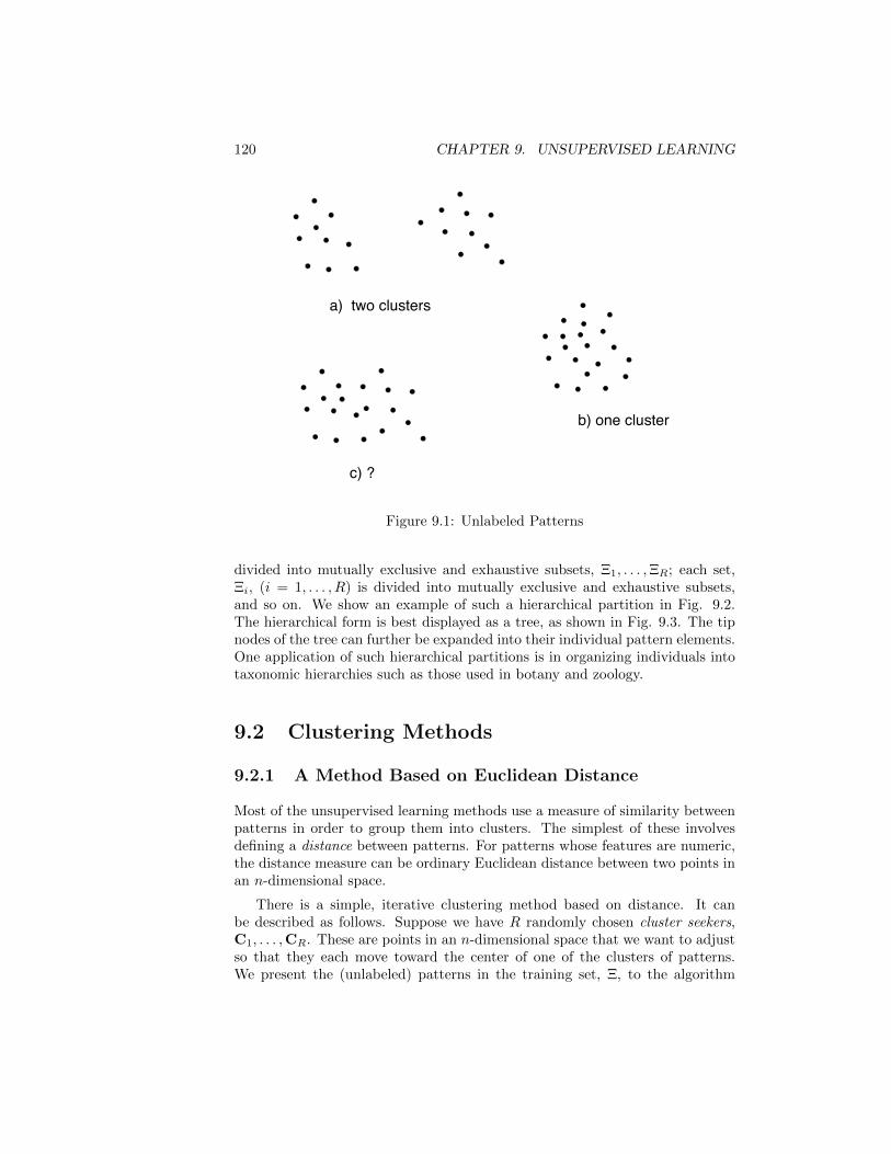
120 CHAPTER 9. UNSUPERVISED LEARNING
a) two clusters
b) one cluster
c) ?
Figure 9.1: Unlabeled Patterns
divided into mutually exclusive and exhaustive subsets, Ξ1, . . . ,ΞR; each set,Ξi, (i = 1, . . . , R) is divided into mutually exclusive and exhaustive subsets,and so on. We show an example of such a hierarchical partition in Fig. 9.2.The hierarchical form is best displayed as a tree, as shown in Fig. 9.3. The tipnodes of the tree can further be expanded into their individual pattern elements.One application of such hierarchical partitions is in organizing individuals intotaxonomic hierarchies such as those used in botany and zoology.
9.2 Clustering Methods
9.2.1 A Method Based on Euclidean Distance
Most of the unsupervised learning methods use a measure of similarity betweenpatterns in order to group them into clusters. The simplest of these involvesdefining a distance between patterns. For patterns whose features are numeric,the distance measure can be ordinary Euclidean distance between two points inan n-dimensional space.
There is a simple, iterative clustering method based on distance. It canbe described as follows. Suppose we have R randomly chosen cluster seekers,C1, . . . ,CR. These are points in an n-dimensional space that we want to adjustso that they each move toward the center of one of the clusters of patterns.We present the (unlabeled) patterns in the training set, Ξ, to the algorithm
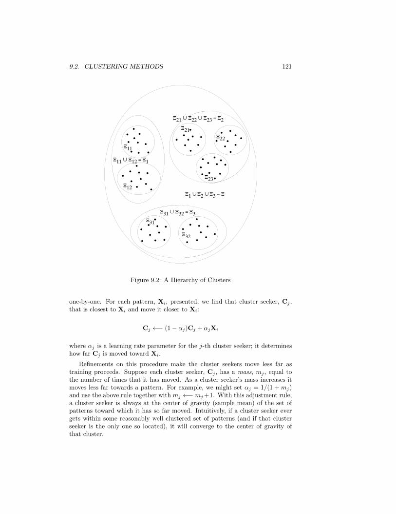
9.2. CLUSTERING METHODS 121
11
12
21
22
23
31
32
11 12 = 1
21 22 23 = 2
31 32 = 3
1 2 3 =
Figure 9.2: A Hierarchy of Clusters
one-by-one. For each pattern, Xi, presented, we find that cluster seeker, Cj ,that is closest to Xi and move it closer to Xi:
Cj ←− (1− αj)Cj + αjXi
where αj is a learning rate parameter for the j-th cluster seeker; it determineshow far Cj is moved toward Xi.
Refinements on this procedure make the cluster seekers move less far astraining proceeds. Suppose each cluster seeker, Cj , has a mass, mj , equal tothe number of times that it has moved. As a cluster seeker’s mass increases itmoves less far towards a pattern. For example, we might set αj = 1/(1 + mj)and use the above rule together with mj ←− mj+1. With this adjustment rule,a cluster seeker is always at the center of gravity (sample mean) of the set ofpatterns toward which it has so far moved. Intuitively, if a cluster seeker evergets within some reasonably well clustered set of patterns (and if that clusterseeker is the only one so located), it will converge to the center of gravity ofthat cluster.
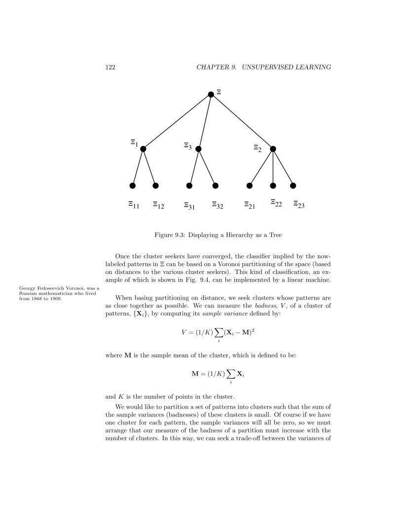
122 CHAPTER 9. UNSUPERVISED LEARNING
2
11 12 31 32 21 22 23
1 3
Figure 9.3: Displaying a Hierarchy as a Tree
Once the cluster seekers have converged, the classifier implied by the now-labeled patterns in Ξ can be based on a Voronoi partitioning of the space (basedon distances to the various cluster seekers). This kind of classification, an ex-ample of which is shown in Fig. 9.4, can be implemented by a linear machine.
Georgy Fedoseevich Voronoi, was aRussian mathematician who livedfrom 1868 to 1909. When basing partitioning on distance, we seek clusters whose patterns are
as close together as possible. We can measure the badness, V , of a cluster ofpatterns, Xi, by computing its sample variance defined by:
V = (1/K)∑i
(Xi −M)2
where M is the sample mean of the cluster, which is defined to be:
M = (1/K)∑i
Xi
and K is the number of points in the cluster.
We would like to partition a set of patterns into clusters such that the sum ofthe sample variances (badnesses) of these clusters is small. Of course if we haveone cluster for each pattern, the sample variances will all be zero, so we mustarrange that our measure of the badness of a partition must increase with thenumber of clusters. In this way, we can seek a trade-off between the variances of
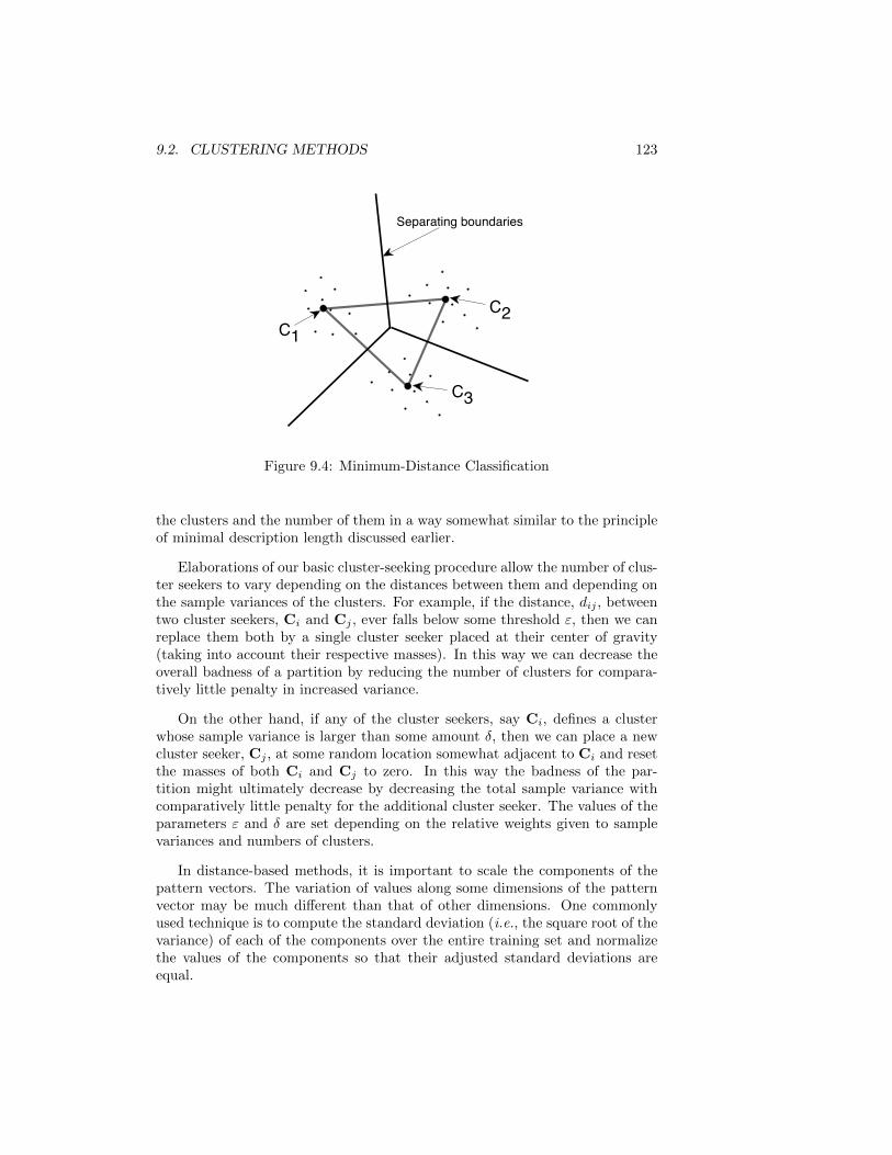
9.2. CLUSTERING METHODS 123
C1C2
C3
Separating boundaries
Figure 9.4: Minimum-Distance Classification
the clusters and the number of them in a way somewhat similar to the principleof minimal description length discussed earlier.
Elaborations of our basic cluster-seeking procedure allow the number of clus-ter seekers to vary depending on the distances between them and depending onthe sample variances of the clusters. For example, if the distance, dij , betweentwo cluster seekers, Ci and Cj , ever falls below some threshold ε, then we canreplace them both by a single cluster seeker placed at their center of gravity(taking into account their respective masses). In this way we can decrease theoverall badness of a partition by reducing the number of clusters for compara-tively little penalty in increased variance.
On the other hand, if any of the cluster seekers, say Ci, defines a clusterwhose sample variance is larger than some amount δ, then we can place a newcluster seeker, Cj , at some random location somewhat adjacent to Ci and resetthe masses of both Ci and Cj to zero. In this way the badness of the par-tition might ultimately decrease by decreasing the total sample variance withcomparatively little penalty for the additional cluster seeker. The values of theparameters ε and δ are set depending on the relative weights given to samplevariances and numbers of clusters.
In distance-based methods, it is important to scale the components of thepattern vectors. The variation of values along some dimensions of the patternvector may be much different than that of other dimensions. One commonlyused technique is to compute the standard deviation (i.e., the square root of thevariance) of each of the components over the entire training set and normalizethe values of the components so that their adjusted standard deviations areequal.
124 CHAPTER 9. UNSUPERVISED LEARNING
9.2.2 A Method Based on Probabilities
Suppose we have a partition of the training set, Ξ, into R mutually exclusiveand exhaustive clusters, C1, . . . , CR. We can decide to which of these clusterssome arbitrary pattern, X, should be assigned by selecting the Ci for whichthe probability, p(Ci|X), is largest, providing p(Ci|X) is larger than some fixedthreshold, δ. As we saw earlier, we can use Bayes rule and base our decision onmaximizing p(X|Ci)p(Ci). Assuming conditional independence of the patterncomponents, xi, the quantity to be maximized is:
S(X, Ci) = p(x1|Ci)p(x2|Ci) · · · p(xn|Ci)p(Ci)
The p(xj |Ci) can be estimated from the sample statistics of the patterns in theclusters and then used in the above expression. (Recall the linear form that thisformula took in the case of binary-valued components.)
We call S(X, Ci) the similarity of X to a cluster, Ci, of patterns. Thus, weassign X to the cluster to which it is most similar, providing the similarity islarger than δ.
Just as before, we can define the sample mean of a cluster, Ci, to be:
Mi = (1/Ki)∑
Xjε Ci
Xj
where Ki is the number of patterns in Ci.
We can base an iterative clustering algorithm on this measure of similarity[Mahadevan & Connell, 1992]. It can be described as follows:
a. Begin with a set of unlabeled patterns Ξ and an empty list, L, of clusters.
b. For the next pattern, X, in Ξ, compute S(X, Ci) for each cluster, Ci.(Initially, these similarities are all zero.) Suppose the largest of thesesimilarities is S(X, Cmax).
(a) If S(X, Cmax) > δ, assign X to Cmax. That is,
Cmax ←− Cmax ∪ X
Update the sample statistics p(x1|Cmax), p(x2|Cmax), . . . , p(xn|Cmax),and p(Cmax) to take the new pattern into account. Go to 3.
(b) If S(X, Cmax) ≤ δ, create a new cluster, Cnew = X and add Cnewto L. Go to 3.
c. Merge any existing clusters, Ci and Cj if (Mi −Mj)2 < ε. Compute
new sample statistics p(x1|Cmerge), p(x2|Cmerge), . . . , p(xn|Cmerge), andp(Cmerge) for the merged cluster, Cmerge = Ci ∪ Cj .
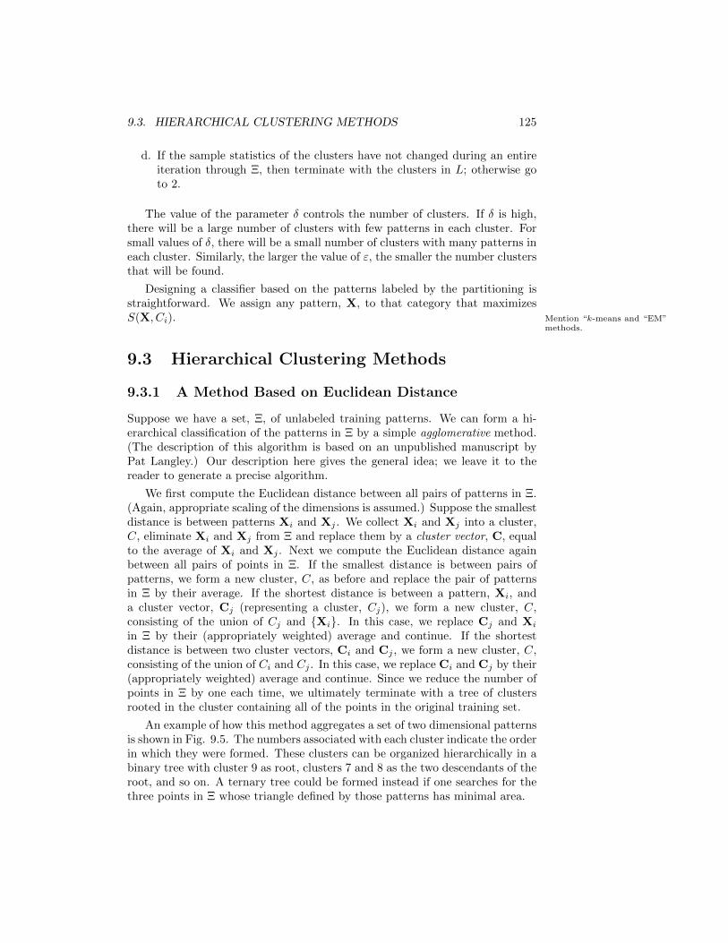
9.3. HIERARCHICAL CLUSTERING METHODS 125
d. If the sample statistics of the clusters have not changed during an entireiteration through Ξ, then terminate with the clusters in L; otherwise goto 2.
The value of the parameter δ controls the number of clusters. If δ is high,there will be a large number of clusters with few patterns in each cluster. Forsmall values of δ, there will be a small number of clusters with many patterns ineach cluster. Similarly, the larger the value of ε, the smaller the number clustersthat will be found.
Designing a classifier based on the patterns labeled by the partitioning isstraightforward. We assign any pattern, X, to that category that maximizesS(X, Ci). Mention “k-means and “EM”
methods.
9.3 Hierarchical Clustering Methods
9.3.1 A Method Based on Euclidean Distance
Suppose we have a set, Ξ, of unlabeled training patterns. We can form a hi-erarchical classification of the patterns in Ξ by a simple agglomerative method.(The description of this algorithm is based on an unpublished manuscript byPat Langley.) Our description here gives the general idea; we leave it to thereader to generate a precise algorithm.
We first compute the Euclidean distance between all pairs of patterns in Ξ.(Again, appropriate scaling of the dimensions is assumed.) Suppose the smallestdistance is between patterns Xi and Xj . We collect Xi and Xj into a cluster,C, eliminate Xi and Xj from Ξ and replace them by a cluster vector, C, equalto the average of Xi and Xj . Next we compute the Euclidean distance againbetween all pairs of points in Ξ. If the smallest distance is between pairs ofpatterns, we form a new cluster, C, as before and replace the pair of patternsin Ξ by their average. If the shortest distance is between a pattern, Xi, anda cluster vector, Cj (representing a cluster, Cj), we form a new cluster, C,consisting of the union of Cj and Xi. In this case, we replace Cj and Xi
in Ξ by their (appropriately weighted) average and continue. If the shortestdistance is between two cluster vectors, Ci and Cj , we form a new cluster, C,consisting of the union of Ci and Cj . In this case, we replace Ci and Cj by their(appropriately weighted) average and continue. Since we reduce the number ofpoints in Ξ by one each time, we ultimately terminate with a tree of clustersrooted in the cluster containing all of the points in the original training set.
An example of how this method aggregates a set of two dimensional patternsis shown in Fig. 9.5. The numbers associated with each cluster indicate the orderin which they were formed. These clusters can be organized hierarchically in abinary tree with cluster 9 as root, clusters 7 and 8 as the two descendants of theroot, and so on. A ternary tree could be formed instead if one searches for thethree points in Ξ whose triangle defined by those patterns has minimal area.
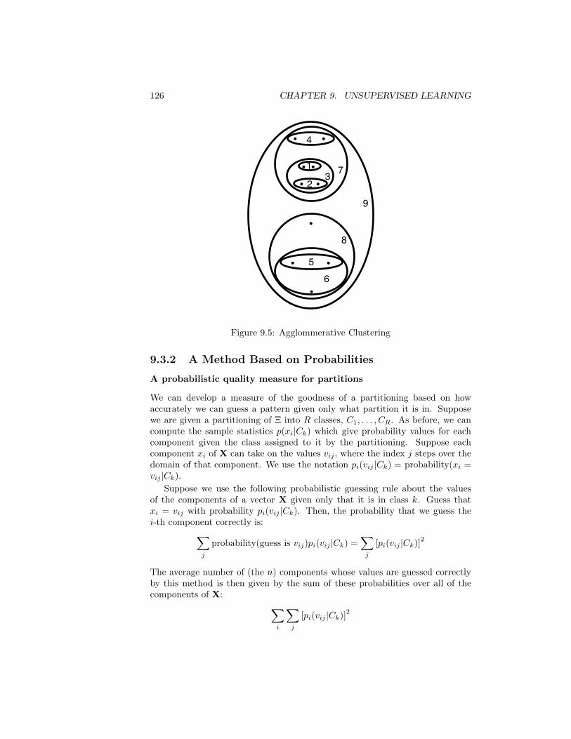
126 CHAPTER 9. UNSUPERVISED LEARNING
1
23
5
4
6
7
8
9
Figure 9.5: Agglommerative Clustering
9.3.2 A Method Based on Probabilities
A probabilistic quality measure for partitions
We can develop a measure of the goodness of a partitioning based on howaccurately we can guess a pattern given only what partition it is in. Supposewe are given a partitioning of Ξ into R classes, C1, . . . , CR. As before, we cancompute the sample statistics p(xi|Ck) which give probability values for eachcomponent given the class assigned to it by the partitioning. Suppose eachcomponent xi of X can take on the values vij , where the index j steps over thedomain of that component. We use the notation pi(vij |Ck) = probability(xi =vij |Ck).
Suppose we use the following probabilistic guessing rule about the valuesof the components of a vector X given only that it is in class k. Guess thatxi = vij with probability pi(vij |Ck). Then, the probability that we guess thei-th component correctly is:∑
j
probability(guess is vij)pi(vij |Ck) =∑j
[pi(vij |Ck)]2
The average number of (the n) components whose values are guessed correctlyby this method is then given by the sum of these probabilities over all of thecomponents of X: ∑
i
∑j
[pi(vij |Ck)]2
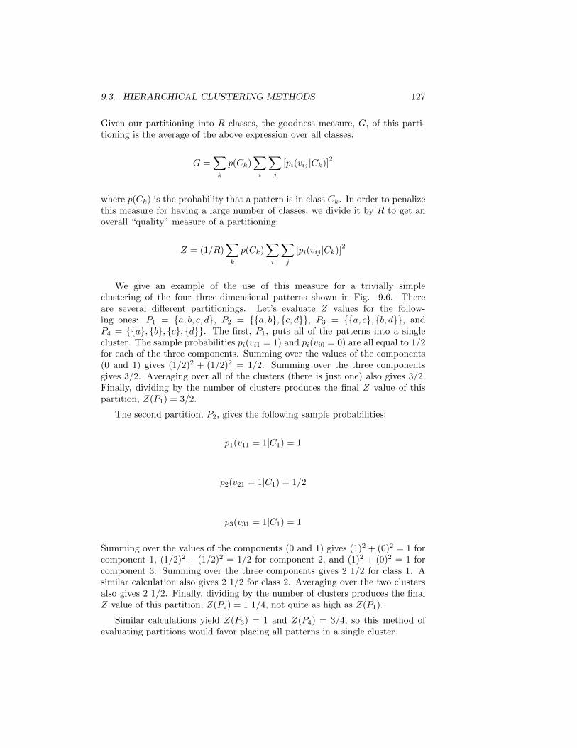
9.3. HIERARCHICAL CLUSTERING METHODS 127
Given our partitioning into R classes, the goodness measure, G, of this parti-tioning is the average of the above expression over all classes:
G =∑k
p(Ck)∑i
∑j
[pi(vij |Ck)]2
where p(Ck) is the probability that a pattern is in class Ck. In order to penalizethis measure for having a large number of classes, we divide it by R to get anoverall “quality” measure of a partitioning:
Z = (1/R)∑k
p(Ck)∑i
∑j
[pi(vij |Ck)]2
We give an example of the use of this measure for a trivially simpleclustering of the four three-dimensional patterns shown in Fig. 9.6. Thereare several different partitionings. Let’s evaluate Z values for the follow-ing ones: P1 = a, b, c, d, P2 = a, b, c, d, P3 = a, c, b, d, andP4 = a, b, c, d. The first, P1, puts all of the patterns into a singlecluster. The sample probabilities pi(vi1 = 1) and pi(vi0 = 0) are all equal to 1/2for each of the three components. Summing over the values of the components(0 and 1) gives (1/2)2 + (1/2)2 = 1/2. Summing over the three componentsgives 3/2. Averaging over all of the clusters (there is just one) also gives 3/2.Finally, dividing by the number of clusters produces the final Z value of thispartition, Z(P1) = 3/2.
The second partition, P2, gives the following sample probabilities:
p1(v11 = 1|C1) = 1
p2(v21 = 1|C1) = 1/2
p3(v31 = 1|C1) = 1
Summing over the values of the components (0 and 1) gives (1)2 + (0)2 = 1 forcomponent 1, (1/2)2 + (1/2)2 = 1/2 for component 2, and (1)2 + (0)2 = 1 forcomponent 3. Summing over the three components gives 2 1/2 for class 1. Asimilar calculation also gives 2 1/2 for class 2. Averaging over the two clustersalso gives 2 1/2. Finally, dividing by the number of clusters produces the finalZ value of this partition, Z(P2) = 1 1/4, not quite as high as Z(P1).
Similar calculations yield Z(P3) = 1 and Z(P4) = 3/4, so this method ofevaluating partitions would favor placing all patterns in a single cluster.
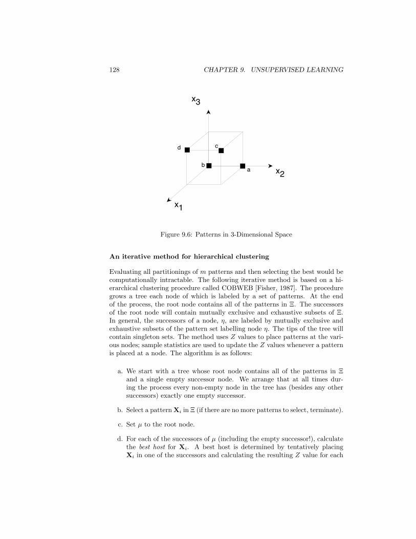
128 CHAPTER 9. UNSUPERVISED LEARNING
x2
x3
x1
ab
cd
Figure 9.6: Patterns in 3-Dimensional Space
An iterative method for hierarchical clustering
Evaluating all partitionings of m patterns and then selecting the best would becomputationally intractable. The following iterative method is based on a hi-erarchical clustering procedure called COBWEB [Fisher, 1987]. The proceduregrows a tree each node of which is labeled by a set of patterns. At the endof the process, the root node contains all of the patterns in Ξ. The successorsof the root node will contain mutually exclusive and exhaustive subsets of Ξ.In general, the successors of a node, η, are labeled by mutually exclusive andexhaustive subsets of the pattern set labelling node η. The tips of the tree willcontain singleton sets. The method uses Z values to place patterns at the vari-ous nodes; sample statistics are used to update the Z values whenever a patternis placed at a node. The algorithm is as follows:
a. We start with a tree whose root node contains all of the patterns in Ξand a single empty successor node. We arrange that at all times dur-ing the process every non-empty node in the tree has (besides any othersuccessors) exactly one empty successor.
b. Select a pattern Xi in Ξ (if there are no more patterns to select, terminate).
c. Set µ to the root node.
d. For each of the successors of µ (including the empty successor!), calculatethe best host for Xi. A best host is determined by tentatively placingXi in one of the successors and calculating the resulting Z value for each

9.3. HIERARCHICAL CLUSTERING METHODS 129
one of these ways of accomodating Xi. The best host corresponds to theassignment with the highest Z value.
e. If the best host is an empty node, η, we place Xi in η, generate an emptysuccessor node of η, generate an empty sibling node of η, and go to 2.
f. If the best host is a non-empty, singleton (tip) node, η, we place Xi in η,create one successor node of η containing the singleton pattern that wasin η, create another successor node of η containing Xi, create an emptysuccessor node of η, create empty successor nodes of the new non-emptysuccessors of η, and go to 2.
g. If the best host is a non-empty, non-singleton node, η, we place Xi in η,set µ to η, and go to 4.
This process is rather sensitive to the order in which patterns are presented.To make the final classification tree less order dependent, the COBWEB proce-dure incorporates node merging and splitting.
Node merging:
It may happen that two nodes having the same parent could be merged withan overall increase in the quality of the resulting classification performed by thesuccessors of that parent. Rather than try all pairs to merge, a good heuristicis to attempt to merge the two best hosts. When such a merging improves theZ value, a new node containing the union of the patterns in the merged nodesreplaces the merged nodes, and the two nodes that were merged are installedas successors of the new node.
Node splitting:
A heuristic for node splitting is to consider replacing the best host among agroup of siblings by that host’s successors. This operation is performed only ifit increases the Z value of the classification performed by a group of siblings.
Example results from COBWEB
We mention two experiments with COBWEB. In the first, the program at-tempted to find two categories (we will call them Class 1 and Class 2) of UnitedStates Senators based on their votes (yes or no) on six issues. After the clus-ters were established, the majority vote in each class was computed. These areshown in the table below.
Issue Class 1 Class 2
Toxic Waste yes noBudget Cuts yes no
SDI Reduction no yesContra Aid yes no
Line-Item Veto yes noMX Production yes no
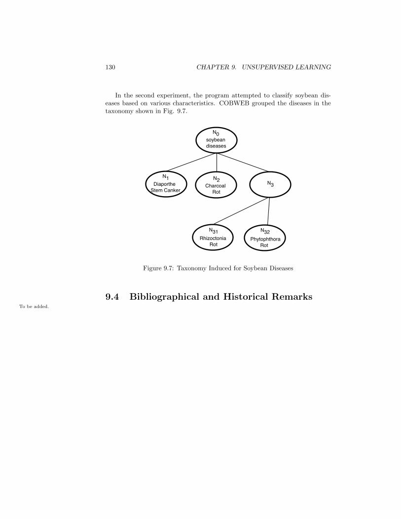
130 CHAPTER 9. UNSUPERVISED LEARNING
In the second experiment, the program attempted to classify soybean dis-eases based on various characteristics. COBWEB grouped the diseases in thetaxonomy shown in Fig. 9.7.
N0soybeandiseases
N1 DiaportheStem Canker
N2Charcoal Rot
N3
N31Rhizoctonia Rot
N32Phytophthora Rot
Figure 9.7: Taxonomy Induced for Soybean Diseases
9.4 Bibliographical and Historical RemarksTo be added.
Chapter 10
Temporal-DifferenceLearning
10.1 Temporal Patterns and Prediction Prob-lems
In this chapter, we consider problems in which we wish to learn to predict thefuture value of some quantity, say z, from an n-dimensional input pattern, X.In many of these problems, the patterns occur in temporal sequence, X1, X2,. . ., Xi, Xi+1, . . ., Xm, and are generated by a dynamical process. Thecomponents of Xi are features whose values are available at time, t = i. Wedistinguish two kinds of prediction problems. In one, we desire to predict thevalue of z at time t = i + 1 based on input Xi for every i. For example, wemight wish to predict some aspects of tomorrow’s weather based on a set ofmeasurements made today. In the other kind of prediction problem, we desireto make a sequence of predictions about the value of z at some fixed time, sayt = m+ 1, based on each of the Xi, i = 1, . . . ,m. For example, we might wishto make a series of predictions about some aspect of the weather on next NewYear’s Day, based on measurements taken every day before New Year’s. Sutton[Sutton, 1988] has called this latter problem, multi-step prediction, and that isthe problem we consider here. In multi-step prediction, we might expect thatthe prediction accuracy should get better and better as i increases toward m.
10.2 Supervised and Temporal-Difference Meth-ods
A training method that naturally suggests itself is to use the actual value ofz at time m + 1 (once it is known) in a supervised learning procedure using a
131
132 CHAPTER 10. TEMPORAL-DIFFERENCE LEARNING
sequence of training patterns, X1, X2, . . ., Xi, Xi+1, . . ., Xm. That is, weseek to learn a function, f , such that f(Xi) is as close as possible to z for each i.Typically, we would need a training set, Ξ, consisting of several such sequences.We will show that a method that is better than supervised learning for someimportant problems is to base learning on the difference between f(Xi+1) andf(Xi) rather than on the difference between z and f(Xi). Such methods involvewhat is called temporal-difference (TD) learning.
We assume that our prediction, f(X), depends on a vector of modifiableweights, W. To make that dependence explicit, we write f(X,W). For su-pervised learning, we consider procedures of the following type: For each Xi,the prediction f(Xi,W) is computed and compared to z, and the learning rule(whatever it is) computes the change, (∆Wi), to be made to W. Then, takinginto account the weight changes for each pattern in a sequence all at once afterhaving made all of the predictions with the old weight vector, we change W asfollows:
W←−W +
m∑i=1
(∆W)i
Whenever we are attempting to minimize the squared error between z andf(Xi,W) by gradient descent, the weight-changing rule for each pattern is:
(∆W)i = c(z − fi)∂fi∂W
where c is a learning rate parameter, fi is our prediction of z, f(Xi,W),at time t = i, and ∂fi
∂W is, by definition, the vector of partial derivatives
( ∂fi∂w1, . . . , ∂fi∂wi
, . . . , ∂fi∂wn) in which the wi are the individual components of W.
(The expression ∂fi∂W is sometimes written ∇Wfi.) The reader will recall that
we used an equivalent expression for (∆W)i in deriving the backpropagationformulas used in training multi-layer neural networks.
The Widrow-Hoff rule results when f(X,W) = X •W. Then:
(∆W)i = c(z − fi)Xi
An interesting form for (∆W)i can be developed if we note that
(z − fi) =
m∑k=i
(fk+1 − fk)
where we define fm+1 = z. Substituting in our formula for (∆W)i yields:
(∆W)i = c(z − fi)∂fi∂W
10.2. SUPERVISED AND TEMPORAL-DIFFERENCE METHODS 133
= c∂fi∂W
m∑k=i
(fk+1 − fk)
In this form, instead of using the difference between a prediction and the valueof z, we use the differences between successive predictions—thus the phrasetemporal-difference (TD) learning.
In the case when f(X,W) = X •W, the temporal difference form of theWidrow-Hoff rule is:
(∆W)i = cXi
m∑k=i
(fk+1 − fk)
One reason for writing (∆W)i in temporal-difference form is to permit aninteresting generalization as follows:
(∆W)i = c∂fi∂W
m∑k=i
λ(k−i)(fk+1 − fk)
where 0 < λ ≤ 1. Here, the λ term gives exponentially decreasing weight todifferences later in time than t = i. When λ = 1, we have the same rule withwhich we began—weighting all differences equally, but as λ→ 0, we weight onlythe (fi+1 − fi) difference. With the λ term, the method is called TD(λ).
It is interesting to compare the two extreme cases:
For TD(0):
(∆W)i = c(fi+1 − fi)∂fi∂W
For TD(1):
(∆W)i = c(z − fi)∂fi∂W
Both extremes can be handled by the same learning mechanism; only the errorterm is different. In TD(0), the error is the difference between successive predic-tions, and in TD(1), the error is the difference between the finally revealed valueof z and the prediction. Intermediate values of λ take into account differentlyweighted differences between future pairs of successive predictions.
Only TD(1) can be considered a pure supervised learning procedure, sensitiveto the final value of z provided by the teacher. For λ < 1, we have various degreesof unsupervised learning, in which the prediction function strives to make eachprediction more like successive ones (whatever they might be). We shall soonsee that these unsupervised procedures result in better learning than do thesupervised ones for an important class of problems.
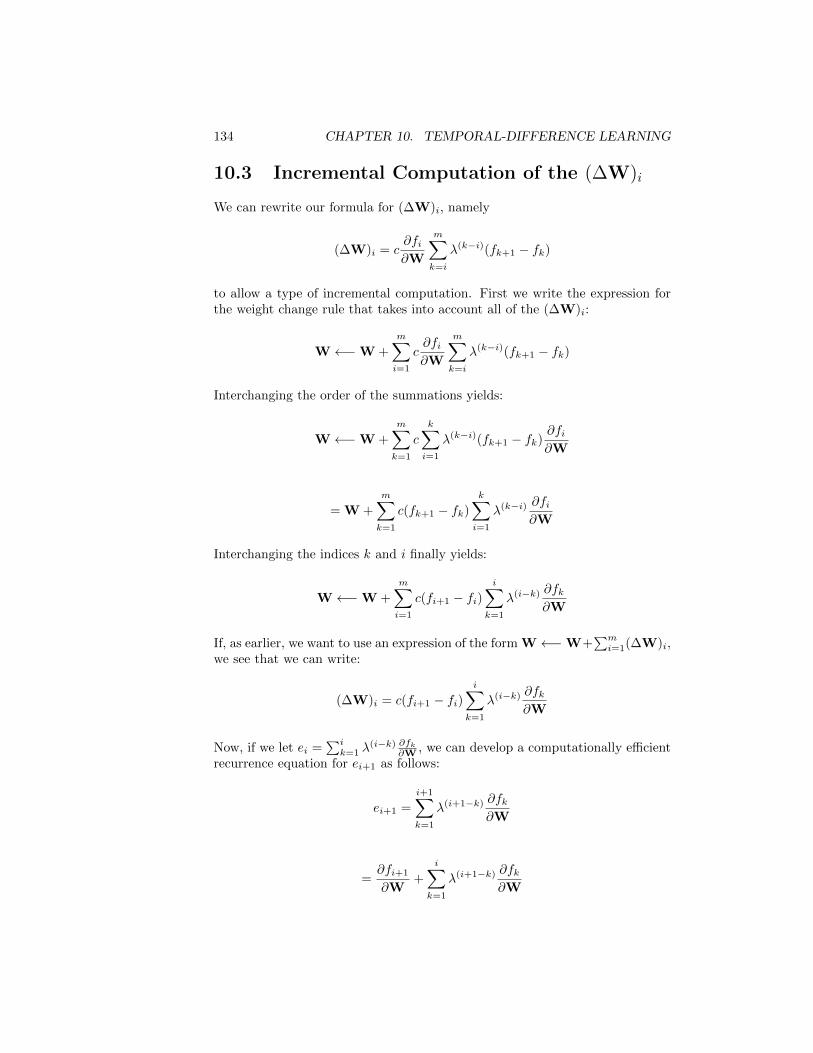
134 CHAPTER 10. TEMPORAL-DIFFERENCE LEARNING
10.3 Incremental Computation of the (∆W)i
We can rewrite our formula for (∆W)i, namely
(∆W)i = c∂fi∂W
m∑k=i
λ(k−i)(fk+1 − fk)
to allow a type of incremental computation. First we write the expression forthe weight change rule that takes into account all of the (∆W)i:
W←−W +
m∑i=1
c∂fi∂W
m∑k=i
λ(k−i)(fk+1 − fk)
Interchanging the order of the summations yields:
W←−W +
m∑k=1
c
k∑i=1
λ(k−i)(fk+1 − fk)∂fi∂W
= W +
m∑k=1
c(fk+1 − fk)
k∑i=1
λ(k−i) ∂fi∂W
Interchanging the indices k and i finally yields:
W←−W +
m∑i=1
c(fi+1 − fi)i∑
k=1
λ(i−k) ∂fk∂W
If, as earlier, we want to use an expression of the form W←−W+∑mi=1(∆W)i,
we see that we can write:
(∆W)i = c(fi+1 − fi)i∑
k=1
λ(i−k) ∂fk∂W
Now, if we let ei =∑ik=1 λ
(i−k) ∂fk∂W , we can develop a computationally efficient
recurrence equation for ei+1 as follows:
ei+1 =
i+1∑k=1
λ(i+1−k) ∂fk∂W
=∂fi+1
∂W+
i∑k=1
λ(i+1−k) ∂fk∂W
10.4. AN EXPERIMENT WITH TD METHODS 135
=∂fi+1
∂W+ λei
Rewriting (∆W)i in these terms, we obtain:
(∆W)i = c(fi+1 − fi)ei
where:
e1 =∂f1
∂W
e2 =∂f2
∂W+ λe1
etc.
Quoting Sutton [Sutton, 1988, page 15] (about a different equation, but thequote applies equally well to this one):
“. . . this equation can be computed incrementally, because each(∆W)i depends only on a pair of successive predictions and on the[weighted] sum of all past values for ∂fi
∂W . This saves substantially onmemory, because it is no longer necessary to individually rememberall past values of ∂fi
∂W .”
10.4 An Experiment with TD Methods
TD prediction methods [especially TD(0)] are well suited to situations in whichthe patterns are generated by a dynamic process. In that case, sequences oftemporally presented patterns contain important information that is ignoredby a conventional supervised method such as the Widrow-Hoff rule. Sutton[Sutton, 1988, page 19] gives an interesting example involving a random walk,which we repeat here. In Fig. 10.1, sequences of vectors, X, are generated asfollows: We start with vector XD; the next vector in the sequence is equallylikely to be one of the adjacent vectors in the diagram. If the next vector isXC (or XE), the next one after that is equally likely to be one of the vectorsadjacent to XC (or XE). When XB is in the sequence, it is equally likely thatthe sequence terminates with z = 0 or that the next vector is XC . Similarly,when XF is in the sequence, it is equally likely that the sequence terminateswith z = 1 or that the next vector is XE . Thus the sequences are random, butthey always start with XD. Some sample sequences are shown in the figure.
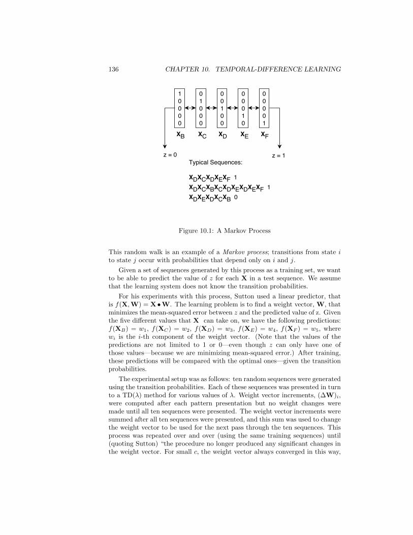
136 CHAPTER 10. TEMPORAL-DIFFERENCE LEARNING
10000
01000
00100
00010
00001
z = 0 z = 1
XB XC XD XE XF
Typical Sequences:
XDXCXDXEXF 1XDXCXBXCXDXEXDXEXF 1XDXEXDXCXB 0
Figure 10.1: A Markov Process
This random walk is an example of a Markov process; transitions from state ito state j occur with probabilities that depend only on i and j.
Given a set of sequences generated by this process as a training set, we wantto be able to predict the value of z for each X in a test sequence. We assumethat the learning system does not know the transition probabilities.
For his experiments with this process, Sutton used a linear predictor, thatis f(X,W) = X •W. The learning problem is to find a weight vector, W, thatminimizes the mean-squared error between z and the predicted value of z. Giventhe five different values that X can take on, we have the following predictions:f(XB) = w1, f(XC) = w2, f(XD) = w3, f(XE) = w4, f(XF ) = w5, wherewi is the i-th component of the weight vector. (Note that the values of thepredictions are not limited to 1 or 0—even though z can only have one ofthose values—because we are minimizing mean-squared error.) After training,these predictions will be compared with the optimal ones—given the transitionprobabilities.
The experimental setup was as follows: ten random sequences were generatedusing the transition probabilities. Each of these sequences was presented in turnto a TD(λ) method for various values of λ. Weight vector increments, (∆W)i,were computed after each pattern presentation but no weight changes weremade until all ten sequences were presented. The weight vector increments weresummed after all ten sequences were presented, and this sum was used to changethe weight vector to be used for the next pass through the ten sequences. Thisprocess was repeated over and over (using the same training sequences) until(quoting Sutton) “the procedure no longer produced any significant changes inthe weight vector. For small c, the weight vector always converged in this way,
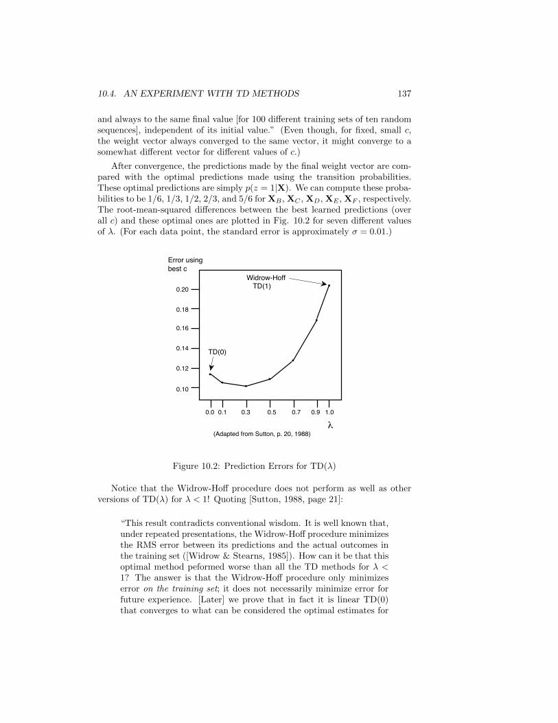
10.4. AN EXPERIMENT WITH TD METHODS 137
and always to the same final value [for 100 different training sets of ten randomsequences], independent of its initial value.” (Even though, for fixed, small c,the weight vector always converged to the same vector, it might converge to asomewhat different vector for different values of c.)
After convergence, the predictions made by the final weight vector are com-pared with the optimal predictions made using the transition probabilities.These optimal predictions are simply p(z = 1|X). We can compute these proba-bilities to be 1/6, 1/3, 1/2, 2/3, and 5/6 for XB , XC , XD, XE , XF , respectively.The root-mean-squared differences between the best learned predictions (overall c) and these optimal ones are plotted in Fig. 10.2 for seven different valuesof λ. (For each data point, the standard error is approximately σ = 0.01.)
0.10
0.12
0.14
0.16
0.18
0.20
0.0 0.1 0.3 0.5 0.7 0.9 1.0
Error usingbest c
Widrow-HoffTD(1)
TD(0)
(Adapted from Sutton, p. 20, 1988)
Figure 10.2: Prediction Errors for TD(λ)
Notice that the Widrow-Hoff procedure does not perform as well as otherversions of TD(λ) for λ < 1! Quoting [Sutton, 1988, page 21]:
“This result contradicts conventional wisdom. It is well known that,under repeated presentations, the Widrow-Hoff procedure minimizesthe RMS error between its predictions and the actual outcomes inthe training set ([Widrow & Stearns, 1985]). How can it be that thisoptimal method peformed worse than all the TD methods for λ <1? The answer is that the Widrow-Hoff procedure only minimizeserror on the training set; it does not necessarily minimize error forfuture experience. [Later] we prove that in fact it is linear TD(0)that converges to what can be considered the optimal estimates for
138 CHAPTER 10. TEMPORAL-DIFFERENCE LEARNING
matching future experience—those consistent with the maximum-likelihood estimate of the underlying Markov process.”
10.5 Theoretical Results
It is possible to analyze the performance of the linear-prediction TD(λ) methodson Markov processes. We state some theorems here without proof.
Theorem 10.1 (Sutton, page 24, 1988) For any absorbing Markov chain,and for any linearly independent set of observation vectors Xi for the non-terminal states, there exists an ε > 0 such that for all positive c < ε and for anyinitial weight vector, the predictions of linear TD(0) (with weight updates aftereach sequence) converge in expected value to the optimal (maximum likelihood)predictions of the true process.
Even though the expected values of the predictions converge, the predictionsthemselves do not converge but vary around their expected values depending ontheir most recent experience. Sutton conjectures that if c is made to approach0 as training progresses, the variance of the predictions will approach 0 also.
Dayan [Dayan, 1992] has extended the result of Theorem 9.1 to TD(λ) forarbitrary λ between 0 and 1. (Also see [Dayan & Sejnowski, 1994].)
10.6 Intra-Sequence Weight Updating
Our standard weight updating rule for TD(λ) methods is:
W←−W +
m∑i=1
c(fi+1 − fi)i∑
k=1
λ(i−k) ∂fk∂W
where the weight update occurs after an entire sequence is observed. To makethe method truly incremental (in analogy with weight updating rules for neuralnets), it would be desirable to change the weight vector after every patternpresentation. The obvious extension is:
Wi+1 ←−Wi + c(fi+1 − fi)i∑
k=1
λ(i−k) ∂fk∂W
where fi+1 is computed before making the weight change; that is, fi+1 =f(Xi+1,Wi). But that would make fi = f(Xi,Wi−1), and such a rule wouldmake the prediction difference, namely (fi+1 − fi), sensitive both to changes inX and changes in W and could lead to instabilities. Instead, we modify the ruleso that, for every pair of predictions, fi+1 = f(Xi+1,Wi) and fi = f(Xi,Wi).This version of the rule has been used in practice with excellent results.
10.6. INTRA-SEQUENCE WEIGHT UPDATING 139
For TD(0) and linear predictors, the rule is:
Wi+1 = Wi + c(fi+1 − fi)Xi
The rule is implemented as follows:
a. Initialize the weight vector, W, arbitrarily.
b. For i = 1, ...,m, do:
(a) fi ←− Xi •W
(We compute fi anew each time through rather than use the valueof fi+1 the previous time through.)
(b) fi+1 ←− Xi+1 •W
(c) di+1 ←− fi+1 − fi(d) W←−W + c di+1Xi
(If fi were computed again with this changed weight vector, its valuewould be closer to fi+1 as desired.)
The linear TD(0) method can be regarded as a technique for training avery simple network consisting of a single dot product unit (and no thresholdor sigmoid function). TD methods can also be used in combination with back-propagation to train neural networks. For TD(0) we change the network weightsaccording to the expression:
Wi+1 = Wi + c(fi+1 − fi)∂fi∂W
The only change that must be made to the standard backpropagation weight-changing rule is that the difference term between the desired output and theoutput of the unit in the final (k-th) layer, namely (d− f (k)), must be replacedby a difference term between successive outputs, (fi+1− fi). This change has adirect effect only on the expression for δ(k) which becomes:
δ(k) = 2(f ′(k) − f (k))f (k)(1− f (k))
where f ′(k) and f (k) are two successive outputs of the network.
The weight changing rule for the i-th weight vector in the j-th layer of weightshas the same form as before, namely:
W(j)i ←−W
(j)i + cδ
(j)i X(j−1)
where the δ(j)i are given recursively by:
δ(j)i = f
(j)i (1− f (j)
i )
mj+1∑l=1
δ(j+1)l w
(j+1)il
and w(j+1)il is the l-th component of the i-th weight vector in the (j+1)-th layer
of weights. Of course, here also it is assumed that f ′(k) and f (k) are computedusing the same weights and then the weights are changed. In the next sectionwe shall see an interesting example of this application of TD learning.
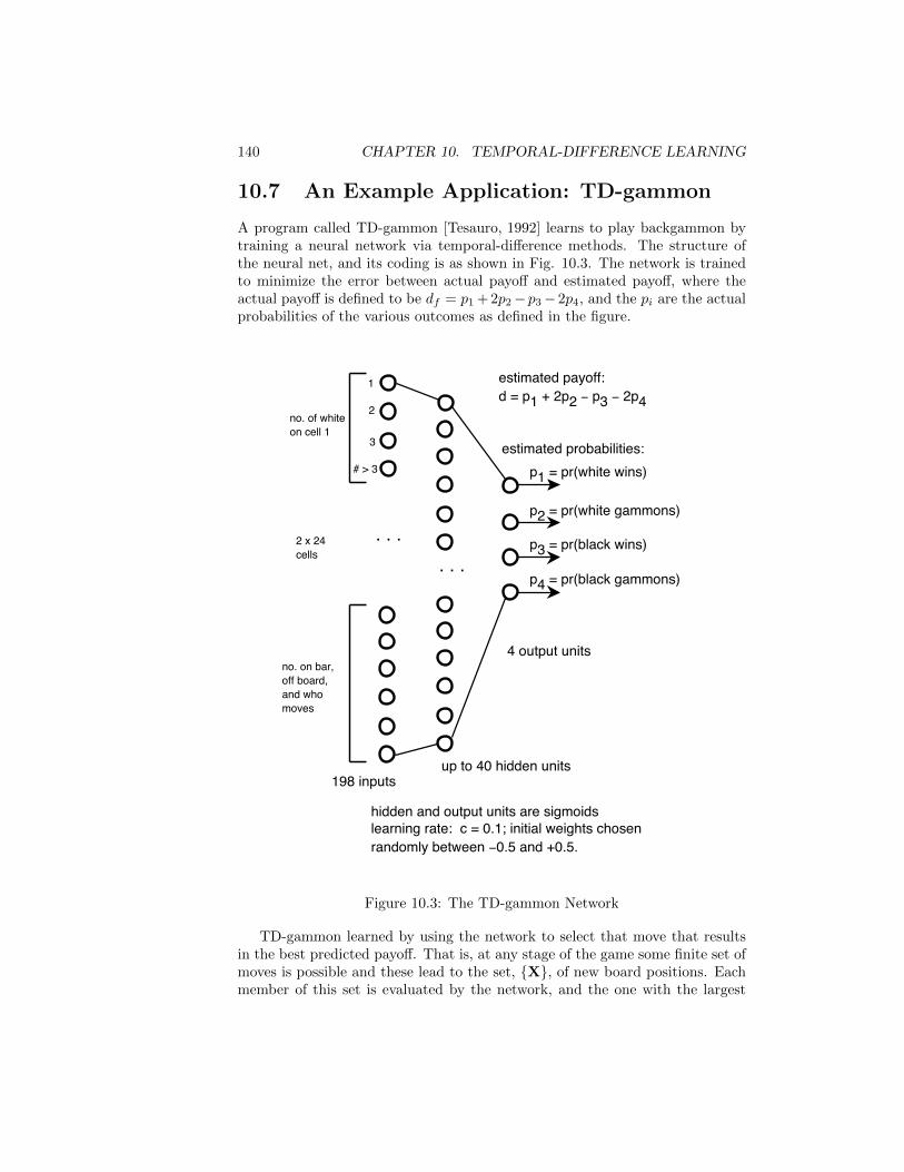
140 CHAPTER 10. TEMPORAL-DIFFERENCE LEARNING
10.7 An Example Application: TD-gammon
A program called TD-gammon [Tesauro, 1992] learns to play backgammon bytraining a neural network via temporal-difference methods. The structure ofthe neural net, and its coding is as shown in Fig. 10.3. The network is trainedto minimize the error between actual payoff and estimated payoff, where theactual payoff is defined to be df = p1 + 2p2− p3− 2p4, and the pi are the actualprobabilities of the various outcomes as defined in the figure.
. . . p3 = pr(black wins)
p4 = pr(black gammons)
p1 = pr(white wins)
p2 = pr(white gammons)
estimated payoff:d = p1 + 2p2 p3 2p4
no. of whiteon cell 1
no. on bar,off board,and whomoves
198 inputs
1
2
3
# > 3
. . .
up to 40 hidden units
2 x 24cells
4 output units
hidden and output units are sigmoidslearning rate: c = 0.1; initial weights chosenrandomly between 0.5 and +0.5.
estimated probabilities:
Figure 10.3: The TD-gammon Network
TD-gammon learned by using the network to select that move that resultsin the best predicted payoff. That is, at any stage of the game some finite set ofmoves is possible and these lead to the set, X, of new board positions. Eachmember of this set is evaluated by the network, and the one with the largest
10.8. BIBLIOGRAPHICAL AND HISTORICAL REMARKS 141
predicted payoff is selected if it is white’s move (and the smallest if it is black’s).The move is made, and the network weights are adjusted to make the predictedpayoff from the original position closer to that of the resulting position.
The weight adjustment procedure combines temporal-difference (TD(λ))learning with backpropagation. If dt is the network’s estimate of the payoffat time t (before a move is made), and dt+1 is the estimate at time t+ 1 (aftera move is made), the weight adjustment rule is:
∆Wt = c(dt+1 − dt)t∑
k=1
λt−k∂dk∂W
where Wt is a vector of all weights in the network at time t, and ∂dk∂W is the
gradient of dk in this weight space. (For a layered, feedforward network, suchas that of TD-gammon, the weight changes for the weight vectors in each layercan be expressed in the usual manner.)
To make the special cases clear, recall that for TD(0), the network would betrained so that, for all t, its output, dt, for input Xt tended toward its expectedoutput, dt+1, for input Xt+1. For TD(1), the network would be trained so that,for all t, its output, dt, for input Xt tended toward the expected final payoff,df , given that input. The latter case is the same as the Widrow-Hoff rule.
After about 200,000 games the following results were obtained. TD-gammon(with 40 hidden units, λ = 0.7, and c = 0.1) won 66.2% of 10,000 games againstSUN Microsystems Gammontool and 55% of 10,000 games against a neuralnetwork trained using expert moves. Commenting on a later version of TD-gammon, incorporating special features as inputs, Tesauro said: “It appears tobe the strongest program ever seen by this author.”
10.8 Bibliographical and Historical RemarksTo be added.

142 CHAPTER 10. TEMPORAL-DIFFERENCE LEARNING
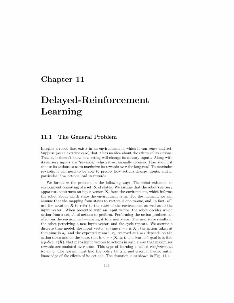
Chapter 11
Delayed-ReinforcementLearning
11.1 The General Problem
Imagine a robot that exists in an environment in which it can sense and act.Suppose (as an extreme case) that it has no idea about the effects of its actions.That is, it doesn’t know how acting will change its sensory inputs. Along withits sensory inputs are “rewards,” which it occasionally receives. How should itchoose its actions so as to maximize its rewards over the long run? To maximizerewards, it will need to be able to predict how actions change inputs, and inparticular, how actions lead to rewards.
We formalize the problem in the following way: The robot exists in anenvironment consisting of a set, S, of states. We assume that the robot’s sensoryapparatus constructs an input vector, X, from the environment, which informsthe robot about which state the environment is in. For the moment, we willassume that the mapping from states to vectors is one-to-one, and, in fact, willuse the notation X to refer to the state of the environment as well as to theinput vector. When presented with an input vector, the robot decides whichaction from a set, A, of actions to perform. Performing the action produces aneffect on the environment—moving it to a new state. The new state results inthe robot perceiving a new input vector, and the cycle repeats. We assume adiscrete time model; the input vector at time t = i is Xi, the action taken atthat time is ai, and the expected reward, ri, received at t = i depends on theaction taken and on the state, that is ri = r(Xi, ai). The learner’s goal is to finda policy, π(X), that maps input vectors to actions in such a way that maximizesrewards accumulated over time. This type of learning is called reinforcementlearning. The learner must find the policy by trial and error; it has no initialknowledge of the effects of its actions. The situation is as shown in Fig. 11.1.
143
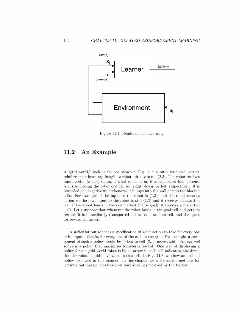
144 CHAPTER 11. DELAYED-REINFORCEMENT LEARNING
Xi
riLearner
Environment
(reward)
(state)
(action)
ai
Figure 11.1: Reinforcement Learning
11.2 An Example
A “grid world,” such as the one shown in Fig. 11.2 is often used to illustratereinforcement learning. Imagine a robot initially in cell (2,3). The robot receivesinput vector (x1, x2) telling it what cell it is in; it is capable of four actions,n, e, s, w moving the robot one cell up, right, down, or left, respectively. It isrewarded one negative unit whenever it bumps into the wall or into the blockedcells. For example, if the input to the robot is (1,3), and the robot choosesaction w, the next input to the robot is still (1,3) and it receives a reward of−1. If the robot lands in the cell marked G (for goal), it receives a reward of+10. Let’s suppose that whenever the robot lands in the goal cell and gets itsreward, it is immediately transported out to some random cell, and the questfor reward continues.
A policy for our robot is a specification of what action to take for every oneof its inputs, that is, for every one of the cells in the grid. For example, a com-ponent of such a policy would be “when in cell (3,1), move right.” An optimalpolicy is a policy that maximizes long-term reward. One way of displaying apolicy for our grid-world robot is by an arrow in each cell indicating the direc-tion the robot should move when in that cell. In Fig. 11.3, we show an optimalpolicy displayed in this manner. In this chapter we will describe methods forlearning optimal policies based on reward values received by the learner.
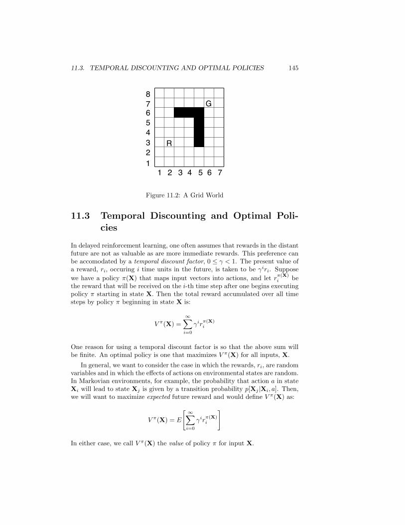
11.3. TEMPORAL DISCOUNTING AND OPTIMAL POLICIES 145
R
G
1 2 3 4 5 6 712345678
Figure 11.2: A Grid World
11.3 Temporal Discounting and Optimal Poli-cies
In delayed reinforcement learning, one often assumes that rewards in the distantfuture are not as valuable as are more immediate rewards. This preference canbe accomodated by a temporal discount factor, 0 ≤ γ < 1. The present value ofa reward, ri, occuring i time units in the future, is taken to be γiri. Suppose
we have a policy π(X) that maps input vectors into actions, and let rπ(X)i be
the reward that will be received on the i-th time step after one begins executingpolicy π starting in state X. Then the total reward accumulated over all timesteps by policy π beginning in state X is:
V π(X) =
∞∑i=0
γirπ(X)i
One reason for using a temporal discount factor is so that the above sum willbe finite. An optimal policy is one that maximizes V π(X) for all inputs, X.
In general, we want to consider the case in which the rewards, ri, are randomvariables and in which the effects of actions on environmental states are random.In Markovian environments, for example, the probability that action a in stateXi will lead to state Xj is given by a transition probability p[Xj |Xi, a]. Then,we will want to maximize expected future reward and would define V π(X) as:
V π(X) = E
[ ∞∑i=0
γirπ(X)i
]
In either case, we call V π(X) the value of policy π for input X.
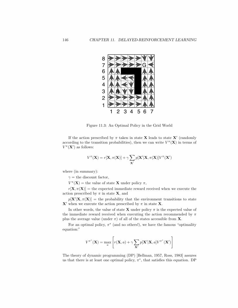
146 CHAPTER 11. DELAYED-REINFORCEMENT LEARNING
R
G
1 2 3 4 5 6 712345678
Figure 11.3: An Optimal Policy in the Grid World
If the action prescribed by π taken in state X leads to state X′ (randomlyaccording to the transition probabilities), then we can write V π(X) in terms ofV π(X′) as follows:
V π(X) = r[X, π(X)] + γ∑X′
p[X′|X, π(X)]V π(X′)
where (in summary):
γ = the discount factor,
V π(X) = the value of state X under policy π,
r[X, π(X)] = the expected immediate reward received when we execute theaction prescribed by π in state X, and
p[X′|X, π(X)] = the probability that the environment transitions to stateX′ when we execute the action prescribed by π in state X.
In other words, the value of state X under policy π is the expected value ofthe immediate reward received when executing the action recommended by πplus the average value (under π) of all of the states accessible from X.
For an optimal policy, π∗ (and no others!), we have the famous “optimalityequation:”
V π∗(X) = max
a
[r(X, a) + γ
∑X′
p[X′|X, a]V π∗(X′)
]
The theory of dynamic programming (DP) [Bellman, 1957, Ross, 1983] assuresus that there is at least one optimal policy, π∗, that satisfies this equation. DP
11.4. Q-LEARNING 147
also provides methods for calculating V π∗(X) and at least one π∗, assuming
that we know the average rewards and the transition probabilities. If we knewthe transition probabilities, the average rewards, and V π
∗(X) for all X and a,
then it would be easy to implement an optimal policy. We would simply selectthat a that maximizes r(X, a) + γ
∑X′ p[X
′|X, a]V π∗(X′). That is,
π∗(X) = arg maxa
[r(X, a) + γ
∑X′
p[X′|X, a]V π∗(X′)
]
But, of course, we are assuming that we do not know these average rewards northe transition probabilities, so we have to find a method that effectively learnsthem.
If we had a model of actions, that is, if we knew for every state, X, andaction a, which state, X′ resulted, then we could use a method called valueiteration to find an optimal policy. Value iteration works as follows: We beginby assigning, randomly, an estimated value V (X) to every state, X. On the i-thstep of the process, suppose we are at state Xi (that is, our input on the i-thstep is Xi), and that the estimated value of state Xi on the i-th step is Vi(Xi).We then select that action a that maximizes the estimated value of the predictedsubsequent state. Suppose this subsequent state having the highest estimatedvalue is X′i. Then we update the estimated value, Vi(Xi), of state Xi as follows:
Vi(X) = (1− ci)Vi−1(X) + ci
[ri + γVi−1(X′i)
]if X = Xi,
= Vi−1(X)
otherwise.
We see that this adjustment moves the value of Vi(Xi) an increment (depend-
ing on ci) closer to[ri + γVi(X
′i)]. Assuming that Vi(X
′i) is a good estimate for
Vi(X′i), then this adjustment helps to make the two estimates more consistent.
Providing that 0 < ci < 1 and that we visit each state infinitely often, thisprocess of value iteration will converge to the optimal values. Discuss synchronous dynamic
programming, asynchronousdynamic programming, and policyiteration.
11.4 Q-Learning
Watkins [Watkins, 1989] has proposed a technique that he calls incrementaldynamic programming. Let a;π stand for the policy that chooses action a once,and thereafter chooses actions according to policy π. We define:
Qπ(X, a) = V a;π(X)
148 CHAPTER 11. DELAYED-REINFORCEMENT LEARNING
Then the optimal value from state X is given by:
V π∗(X) = max
aQπ∗(X, a)
This equation holds only for an optimal policy, π∗. The optimal policy is givenby:
π∗(X) = arg maxa
Qπ∗(X, a)
Note that if an action a makes Qπ(X, a) larger than V π(X), then we can improveπ by changing it so that π(X) = a. Making such a change is the basis for apowerful learning rule that we shall describe shortly.
Suppose action a in state X leads to state X′. Then using the definitions ofQ and V , it is easy to show that:
Qπ(X, a) = r(X, a) + γE[V π(X′)]
where r(X, a) is the average value of the immediate reward received when weexecute action a in state X. For an optimal policy (and no others), we haveanother version of the optimality equation in terms of Q values:
Qπ∗(X, a) = max
a
[r(X, a) + γE
[Qπ∗(X′, a)
]]for all actions, a, and states, X. Now, if we had the optimal Q values (for alla and X), then we could implement an optimal policy simply by selecting thataction that maximized r(X, a) + γE
[Qπ∗(X′, a)
].
That is,
π∗(X) = arg maxa
[r(X, a) + γE
[Qπ∗(X′, a)
]]Watkins’ proposal amounts to a TD(0) method of learning the Q values.
We quote (with minor notational changes) from [Watkins & Dayan, 1992, page281]:
“In Q-Learning, the agent’s experience consists of a sequence of dis-tinct stages or episodes. In the i-th episode, the agent:
• observes its current state Xi,
• selects [using the method described below] and performs anaction ai,
• observes the subsequent state X′i,
• receives an immediate reward ri, and
11.4. Q-LEARNING 149
• adjusts its Qi−1 values using a learning factor ci, according to:
Qi(X, a) = (1− ci)Qi−1(X, a) + ci[ri + γVi−1(X′i)]
if X = Xi and a = ai,
= Qi−1(X, a)
otherwise,
where
Vi−1(X′) = maxb
[Qi−1(X′, b)]
is the best the agent thinks it can do from state X′. . . . Theinitial Q values, Q0(X, a), for all states and actions are assumedgiven.”
Using the current Q values, Qi(X, a), the agent always selects that actionthat maximizes Qi(X, a). Note that only the Q value corresponding to thestate just exited and the action just taken is adjusted. And that Q value isadjusted so that it is closer (by an amount determined by ci) to the sum ofthe immediate reward plus the discounted maximum (over all actions) of the Qvalues of the state just entered. If we imagine the Q values to be predictions ofultimate (infinite horizon) total reward, then the learning procedure describedabove is exactly a TD(0) method of learning how to predict these Q values.Q learning strengthens the usual TD methods, however, because TD (appliedto reinforcement problems using value iteration) requires a one-step lookahead,using a model of the effects of actions, whereas Q learning does not.
A convenient notation (proposed by [Schwartz, 1993]) for representing thechange in Q value is:
Q(X, a)β←− r + γV (X′)
where Q(X, a) is the new Q value for input X and action a, r is the immediatereward when action a is taken in response to input X, V (X′) is the maximum(over all actions) of the Q value of the state next reached when action a is takenfrom state X, and β is the fraction of the way toward which the new Q value,Q(X, a), is adjusted to equal r + γV (X′).
Watkins and Dayan [Watkins & Dayan, 1992] prove that, under certain con-ditions, the Q values computed by this learning procedure converge to optimalones (that is, to ones on which an optimal policy can be based).
We define ni(X, a) as the index (episode number) of the i-th time that actiona is tried in state X. Then, we have:
150 CHAPTER 11. DELAYED-REINFORCEMENT LEARNING
Theorem 11.1 (Watkins and Dayan) For Markov problems with states Xand actions a, and given bounded rewards |rn| ≤ R, learning rates 0 ≤ cn < 1,and
∞∑i=0
cni(X,a) =∞,∞∑i=0
[cni(X,a)
]2<∞
for all X and a, then
Qn(X, a) → Q∗n(X, a) as n → ∞, for all X and a, with probability 1, whereQ∗n(X, a) corresponds to the Q values of an optimal policy.
Again, we quote from [Watkins & Dayan, 1992, page 281]:
“The most important condition implicit in the convergence theorem. . . is that the sequence of episodes that forms the basis of learningmust include an infinite number of episodes for each starting stateand action. This may be considered a strong condition on the waystates and actions are selected—however, under the stochastic con-ditions of the theorem, no method could be guaranteed to find anoptimal policy under weaker conditions. Note, however, that theepisodes need not form a continuous sequence—that is the X′ of oneepisode need not be the X of the next episode.”
The relationships among Q learning, dynamic programming, and controlare very well described in [Barto, Bradtke, & Singh, 1994]. Q learning is bestthought of as a stochastic approximation method for calculating the Q values.Although the definition of the optimal Q values for any state depends recursivelyon expected values of the Q values for subsequent states (and on the expectedvalues of rewards), no expected values are explicitly computed by the procedure.Instead, these values are approximated by iterative sampling using the actualstochastic mechanism that produces successor states.
11.5 Discussion, Limitations, and Extensions ofQ-Learning
11.5.1 An Illustrative Example
The Q-learning procedure requires that we maintain a table of Q(X, a) valuesfor all state-action pairs. In the grid world that we described earlier, such atable would not be excessively large. We might start with random entries in thetable; a portion of such an intial table might be as follows:
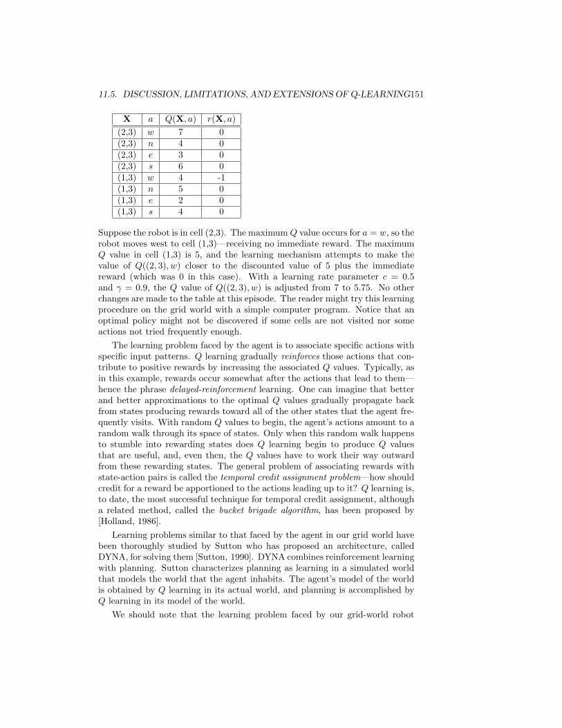
11.5. DISCUSSION, LIMITATIONS, AND EXTENSIONS OF Q-LEARNING151
X a Q(X, a) r(X, a)
(2,3) w 7 0(2,3) n 4 0(2,3) e 3 0(2,3) s 6 0(1,3) w 4 -1(1,3) n 5 0(1,3) e 2 0(1,3) s 4 0
Suppose the robot is in cell (2,3). The maximumQ value occurs for a = w, so therobot moves west to cell (1,3)—receiving no immediate reward. The maximumQ value in cell (1,3) is 5, and the learning mechanism attempts to make thevalue of Q((2, 3), w) closer to the discounted value of 5 plus the immediatereward (which was 0 in this case). With a learning rate parameter c = 0.5and γ = 0.9, the Q value of Q((2, 3), w) is adjusted from 7 to 5.75. No otherchanges are made to the table at this episode. The reader might try this learningprocedure on the grid world with a simple computer program. Notice that anoptimal policy might not be discovered if some cells are not visited nor someactions not tried frequently enough.
The learning problem faced by the agent is to associate specific actions withspecific input patterns. Q learning gradually reinforces those actions that con-tribute to positive rewards by increasing the associated Q values. Typically, asin this example, rewards occur somewhat after the actions that lead to them—hence the phrase delayed-reinforcement learning. One can imagine that betterand better approximations to the optimal Q values gradually propagate backfrom states producing rewards toward all of the other states that the agent fre-quently visits. With random Q values to begin, the agent’s actions amount to arandom walk through its space of states. Only when this random walk happensto stumble into rewarding states does Q learning begin to produce Q valuesthat are useful, and, even then, the Q values have to work their way outwardfrom these rewarding states. The general problem of associating rewards withstate-action pairs is called the temporal credit assignment problem—how shouldcredit for a reward be apportioned to the actions leading up to it? Q learning is,to date, the most successful technique for temporal credit assignment, althougha related method, called the bucket brigade algorithm, has been proposed by[Holland, 1986].
Learning problems similar to that faced by the agent in our grid world havebeen thoroughly studied by Sutton who has proposed an architecture, calledDYNA, for solving them [Sutton, 1990]. DYNA combines reinforcement learningwith planning. Sutton characterizes planning as learning in a simulated worldthat models the world that the agent inhabits. The agent’s model of the worldis obtained by Q learning in its actual world, and planning is accomplished byQ learning in its model of the world.
We should note that the learning problem faced by our grid-world robot
152 CHAPTER 11. DELAYED-REINFORCEMENT LEARNING
could be modified to have several places in the grid that give positive rewards.This possibility presents an interesting way to generalize the classical notion ofa “goal” in AI planning systems—even in those that do no learning. Instead ofrepresenting a goal as a condition to be achieved, we represent a “goal struc-ture” as a set of rewards to be given for achieving various conditions. Then,the generalized “goal” becomes maximizing discounted future reward instead ofsimply achieving some particular condition. This generalization can be made toencompass so-called goals of maintenance and goals of avoidance. The exam-ple presented above included avoiding bumping into the grid-world boundary.A goal of maintenance, of a particular state, could be expressed in terms of areward that was earned whenever the agent was in that state and performed anaction that transitioned back to that state in one step.
11.5.2 Using Random Actions
When the next pattern presentation in a sequence of patterns is the one causedby the agent’s own action in response to the last pattern, we have what is calledan on-line learning method. In Watkins and Dayan’s terminology, in on-linelearning the episodes form a continous sequence. As already mentioned, theconvergence theorem for Q learning does not require on-line learning; indeed,special precautions must be taken to ensure that on-line learning meets theconditions of the theorem. If on-line learning discovers some good paths torewards, the agent may fixate on these and never discover a policy that leadsto a possibly greater long-term reward. In reinforcement learning phraseology,this problem is referred to as the problem of exploitation (of already learnedbehavior) versus exploration (of possibly better behavior).
One way to force exploration is to perform occasional random actions (in-stead of that single action prescribed by the current Q values). For example,in the grid-world problem, one could imagine selecting an action randomly ac-cording to a probability distribution over the actions (n, e, s, and w). Thisdistribution, in turn, could depend on the Q values. For example, we mightfirst find that action prescribed by the Q values and then choose that actionwith probability 1/2, choose the two orthogonal actions with probability 3/16each, and choose the opposite action with probability 1/8. This policy might bemodified by “simulated annealing” which would gradually increase the probabil-ity of the action prescribed by the Q values more and more as time goes on. Thisstrategy would favor exploration at the beginning of learning and exploitationlater.
Other methods, also, have been proposed for dealing with exploration, in-cluding making unvisited states intrinsically rewarding and using an “intervalestimate,” which is related to the uncertainty in the estimate of a state’s value[Kaelbling, 1993].
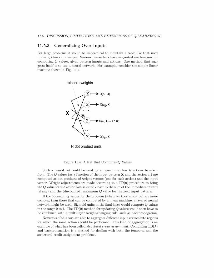
11.5. DISCUSSION, LIMITATIONS, AND EXTENSIONS OF Q-LEARNING153
11.5.3 Generalizing Over Inputs
For large problems it would be impractical to maintain a table like that usedin our grid-world example. Various researchers have suggested mechanisms forcomputing Q values, given pattern inputs and actions. One method that sug-gests itself is to use a neural network. For example, consider the simple linearmachine shown in Fig. 11.4.
X. . .
. . .
trainable weights
Wi
R dot product units
Q(ai, X) = X . Wi
Q(a1, X)
Q(a2, X)
Q(aR, X)
Figure 11.4: A Net that Computes Q Values
Such a neural net could be used by an agent that has R actions to selectfrom. The Q values (as a function of the input pattern X and the action ai) arecomputed as dot products of weight vectors (one for each action) and the inputvector. Weight adjustments are made according to a TD(0) procedure to bringthe Q value for the action last selected closer to the sum of the immediate reward(if any) and the (discounted) maximum Q value for the next input pattern.
If the optimum Q values for the problem (whatever they might be) are morecomplex than those that can be computed by a linear machine, a layered neuralnetwork might be used. Sigmoid units in the final layer would compute Q valuesin the range 0 to 1. The TD(0) method for updating Q values would then have tobe combined with a multi-layer weight-changing rule, such as backpropagation.
Networks of this sort are able to aggregate different input vectors into regionsfor which the same action should be performed. This kind of aggregation is anexample of what has been called structural credit assignment. Combining TD(λ)and backpropagation is a method for dealing with both the temporal and thestructural credit assignment problems.
154 CHAPTER 11. DELAYED-REINFORCEMENT LEARNING
Interesting examples of delayed-reinforcement training of simulated andactual robots requiring structural credit assignment have been reported by[Lin, 1992, Mahadevan & Connell, 1992].
11.5.4 Partially Observable States
So far, we have identified the input vector, X, with the actual state of the envi-ronment. When the input vector results from an agent’s perceptual apparatus(as we assume it does), there is no reason to suppose that it uniquely identifiesthe environmental state. Because of inevitable perceptual limitations, severaldifferent environmental states might give rise to the same input vector. Thisphenomenon has been referred to as perceptual aliasing. With perceptual alias-ing, we can no longer guarantee that Q learning will result in even useful actionpolicies, let alone optimal ones. Several researchers have attempted to deal withthis problem using a variety of methods including attempting to model “hid-den” states by using internal memory [Lin, 1993]. That is, if some aspect ofthe environment cannot be sensed currently, perhaps it was sensed once andcan be remembered by the agent. When such is the case, we no longer have aMarkov problem; that is, the next X vector, given any action, may depend ona sequence of previous ones rather than just the immediately preceding one. Itmight be possible to reinstate a Markov framework (over the X’s) if X includesnot only current sensory precepts but information from the agent’s memory.
11.5.5 Scaling Problems
Several difficulties have so far prohibited wide application of reinforcement learn-ing to large problems. (The TD-gammon program, mentioned in the last chap-ter, is probably unique in terms of success on a high-dimensional problem.)We have already touched on some difficulties; these and others are summarizedbelow with references to attempts to overcome them.
a. Exploration versus exploitation.
• use random actions
• favor states not visited recently
• separate the learning phase from the use phase
• employ a teacher to guide exploration
b. Slow time to convergence
• combine learning with prior knowledge; use estimates of Q values(rather than random values) initially
• use a hierarchy of actions; learn primitive actions first and freeze theuseful sequences into macros and then learn how to use the macros

11.6. BIBLIOGRAPHICAL AND HISTORICAL REMARKS 155
• employ a teacher; use graded “lessons”—starting near the rewardsand then backing away, and use examples of good behavior [Lin, 1992]
• use more efficient computations; e.g. do several updates per episode[Moore & Atkeson, 1993]
c. Large state spaces
• use hand-coded features
• use neural networks
• use nearest-neighbor methods [Moore, 1990]
d. Temporal discounting problems. Using small γ can make the learner toogreedy for present rewards and indifferent to the future; but using large γslows down learning.
• use a learning method based on average rewards [Schwartz, 1993]
e. No “transfer” of learning . What is learned depends on the reward struc-ture; if the rewards change, learning has to start over.
• Separate the learning into two parts: learn an “action model” whichpredicts how actions change states (and is constant over all prob-lems), and then learn the “values” of states by reinforcement learn-ing for each different set of rewards. Sometimes the reinforcementlearning part can be replaced by a “planner” that uses the actionmodel to produce plans to achieve goals.
Also see other articles in the special issue on reinforcement learning: MachineLearning, 8, May, 1992.
11.6 Bibliographical and Historical RemarksTo be added.

156 CHAPTER 11. DELAYED-REINFORCEMENT LEARNING
Chapter 12
Explanation-BasedLearning
12.1 Deductive Learning
In the learning methods studied so far, typically the training set does not ex-haust the version space. Using logical terminology, we could say that the classi-fier’s output does not logically follow from the training set. In this sense, thesemethods are inductive. In logic, a deductive system is one whose conclusionslogically follow from a set of input facts, if the system is sound.1
To contrast inductive with deductive systems in a logical setting, supposewe have a set of facts (the training set) that includes the following formulas:
Round(Obj1), Round(Obj2), Round(Obj3), Round(Obj4),
Ball(Obj1), Ball(Obj2), Ball(Obj3), Ball(Obj4)
A learning system that forms the conclusion (∀x)[Ball(x) ⊃ Round(x)] is in-ductive. This conclusion may be useful (if there are no facts of the formBall(σ) ∧ ¬Round(σ)), but it does not logically follow from the facts. On theother hand, if we had the facts Green(Obj5) and Green(Obj5) ⊃ Round(Obj5),then we could logically conclude Round(Obj5). Making this conclusion and sav-ing it is an instance of deductive learning—a topic we study in this chapter.
Suppose that some logical proposition, φ, logically follows from some set offacts, ∆. Under what circumstances might we say that the process of deducingφ from ∆ results in our learning φ? In a sense, we implicitly knew φ all along,since it was inherent in knowing ∆. Yet, φ might not be obvious given ∆, and
1Logical reasoning systems that are not sound, for example those using non-monotonicreasoning, themselves might produce inductive conclusions that do not logically follow fromthe input facts.
157
158 CHAPTER 12. EXPLANATION-BASED LEARNING
the deduction process to establish φ might have been arduous. Rather than haveto deduce φ again, we might want to save it, perhaps along with its deduction,in case it is needed later. Shouldn’t that process count as learning? Dietterich[Dietterich, 1990] has called this type of learning speed-up learning.
Strictly speaking, speed-up learning does not result in a system being able tomake decisions that, in principle, could not have been made before the learningtook place. Speed-up learning simply makes it possible to make those decisionsmore efficiently. But, in practice, this type of learning might make possiblecertain decisions that might otherwise have been infeasible.
To take an extreme case, a chess player can be said to learn chess even thoughoptimal play is inherent in the rules of chess. On the surface, there seems to beno real difference between the experience-based hypotheses that a chess playermakes about what constitutes good play and the kind of learning we have beenstudying so far.
As another example, suppose we are given some theorems about geometryand are asked to prove that the sum of the angles of a right triangle is 180degrees. Let us further suppose that the proof we constructed did not dependon the given triangle being a right triangle; in that case we can learn a moregeneral fact. The learning technique that we are going to study next is relatedto this example. It is called explanation-based learning (EBL). EBL can bethought of as a process in which implicit knowledge is converted into explicitknowledge.
In EBL, we specialize parts of a domain theory to explain a particular ex-ample, then we generalize the explanation to produce another element of thedomain theory that will be useful on similar examples. This process is illustratedin Fig. 12.1.
12.2 Domain Theories
Two types of information were present in the inductive methods we have studied:the information inherent in the training samples and the information about thedomain that is implied by the “bias” (for example, the hypothesis set from whichwe choose functions). The learning methods are successful only if the hypothesisset is appropriate for the problem. Typically, the smaller the hypothesis set (thatis, the more a priori information we have about the function being sought), theless dependent we are on information being supplied by a training set (thatis, fewer samples). A priori information about a problem can be expressed inseveral ways. The methods we have studied so far restrict the hypotheses in arather direct way. A less direct method involves making assertions in a logicallanguage about the property we are trying to learn. A set of such assertions isusually called a “domain theory.”
Suppose, for example, that we wanted to classify people according to whetheror not they were good credit risks. We might represent a person by a set ofproperties (income, marital status, type of employment, etc.), assemble such
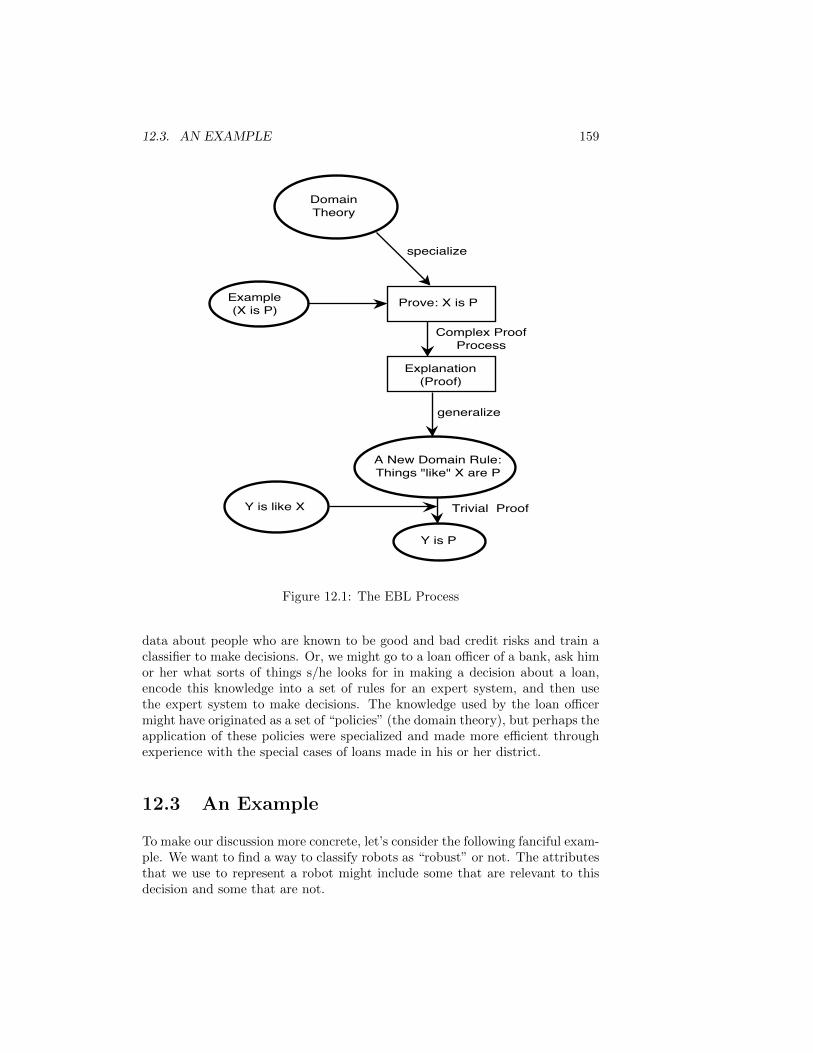
12.3. AN EXAMPLE 159
DomainTheory
Example(X is P)
Prove: X is P
specialize
Explanation(Proof)
generalize
A New Domain Rule:Things "like" X are P
Y is like X
Complex ProofProcess
Trivial Proof
Y is P
Figure 12.1: The EBL Process
data about people who are known to be good and bad credit risks and train aclassifier to make decisions. Or, we might go to a loan officer of a bank, ask himor her what sorts of things s/he looks for in making a decision about a loan,encode this knowledge into a set of rules for an expert system, and then usethe expert system to make decisions. The knowledge used by the loan officermight have originated as a set of “policies” (the domain theory), but perhaps theapplication of these policies were specialized and made more efficient throughexperience with the special cases of loans made in his or her district.
12.3 An Example
To make our discussion more concrete, let’s consider the following fanciful exam-ple. We want to find a way to classify robots as “robust” or not. The attributesthat we use to represent a robot might include some that are relevant to thisdecision and some that are not.
160 CHAPTER 12. EXPLANATION-BASED LEARNING
Suppose we have a domain theory of logical sentences that taken together,help to define whether or not a robot can be classified as robust. (The samedomain theory may be useful for several other purposes also, but among otherthings, it describes the concept “robust.”)
In this example, let’s suppose that our domain theory includes the sentences:
Fixes(u, u) ⊃ Robust(u)
(An individual that can fix itself is robust.)
Sees(x, y) ∧Habile(x) ⊃ Fixes(x, y)
(A habile individual that can see another entity can fix that entity.)
Robot(w) ⊃ Sees(w,w)
(All robots can see themselves.)
R2D2(x) ⊃ Habile(x)
(R2D2-class individuals are habile.)
C3PO(x) ⊃ Habile(x)
(C3PO-class individuals are habile.)
. . .
(By convention, variables are assumed to be universally quantified.) We coulduse theorem-proving methods operating on this domain theory to concludewhether certain robots are robust. These methods might be computationallyquite expensive because extensive search may have to be performed to derive aconclusion. But after having found a proof for some particular robot, we mightbe able to derive some new sentence whose use allows a much faster conclusion.
We next show how such a new rule might be derived in this example. Supposewe are given a number of facts about Num5, such as:
Robot(Num5)
R2D2(Num5)
Age(Num5, 5)
Manufacturer(Num5, GR)
. . .
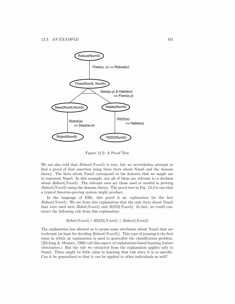
12.3. AN EXAMPLE 161
Fixes(u, u) => Robust(u)
Robust(Num5)
Fixes(Num5, Num5)
Sees(Num5,Num5) Habile(Num5)
Sees(x,y) & Habile(x) => Fixes(x,y)
Robot(w) => Sees(w,w)
Robot(Num5)
R2D2(x) => Habile(x)
R2D2(Num5)
Figure 12.2: A Proof Tree
We are also told that Robust(Num5) is true, but we nevertheless attempt tofind a proof of that assertion using these facts about Num5 and the domaintheory. The facts about Num5 correspond to the features that we might useto represent Num5. In this example, not all of them are relevant to a decisionabout Robust(Num5). The relevant ones are those used or needed in provingRobust(Num5) using the domain theory. The proof tree in Fig. 12.2 is one thata typical theorem-proving system might produce.
In the language of EBL, this proof is an explanation for the factRobust(Num5). We see from this explanation that the only facts about Num5that were used were Robot(Num5) and R2D2(Num5). In fact, we could con-struct the following rule from this explanation:
Robot(Num5) ∧R2D2(Num5) ⊃ Robust(Num5)
The explanation has allowed us to prune some attributes about Num5 that areirrelevant (at least for deciding Robust(Num5)). This type of pruning is the firstsense in which an explanation is used to generalize the classification problem.([DeJong & Mooney, 1986] call this aspect of explanation-based learning featureelimination.) But the rule we extracted from the explanation applies only toNum5. There might be little value in learning that rule since it is so specific.Can it be generalized so that it can be applied to other individuals as well?
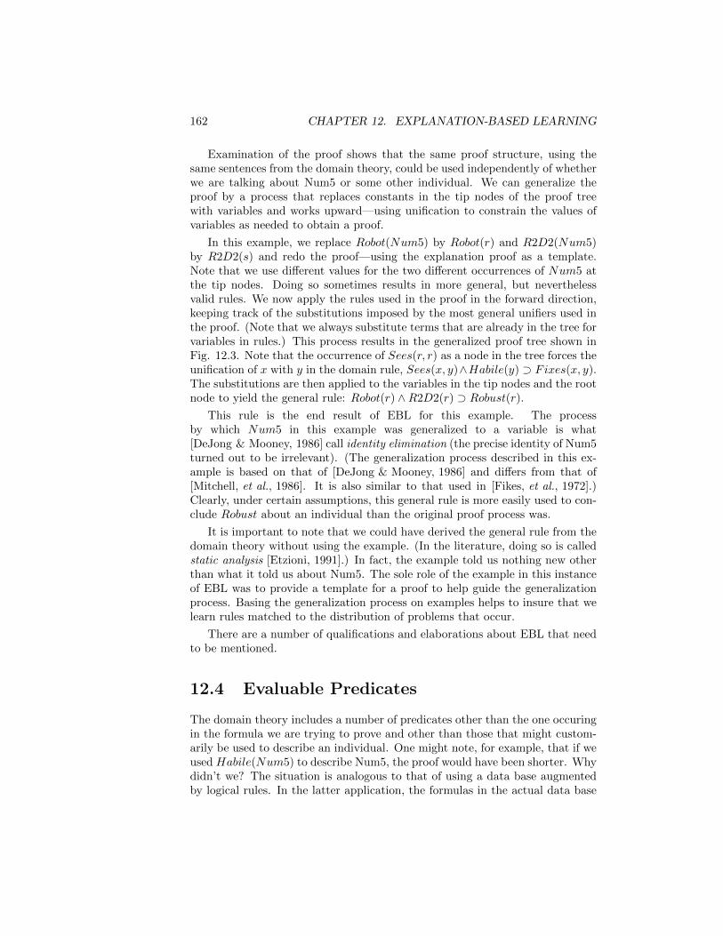
162 CHAPTER 12. EXPLANATION-BASED LEARNING
Examination of the proof shows that the same proof structure, using thesame sentences from the domain theory, could be used independently of whetherwe are talking about Num5 or some other individual. We can generalize theproof by a process that replaces constants in the tip nodes of the proof treewith variables and works upward—using unification to constrain the values ofvariables as needed to obtain a proof.
In this example, we replace Robot(Num5) by Robot(r) and R2D2(Num5)by R2D2(s) and redo the proof—using the explanation proof as a template.Note that we use different values for the two different occurrences of Num5 atthe tip nodes. Doing so sometimes results in more general, but neverthelessvalid rules. We now apply the rules used in the proof in the forward direction,keeping track of the substitutions imposed by the most general unifiers used inthe proof. (Note that we always substitute terms that are already in the tree forvariables in rules.) This process results in the generalized proof tree shown inFig. 12.3. Note that the occurrence of Sees(r, r) as a node in the tree forces theunification of x with y in the domain rule, Sees(x, y)∧Habile(y) ⊃ Fixes(x, y).The substitutions are then applied to the variables in the tip nodes and the rootnode to yield the general rule: Robot(r) ∧R2D2(r) ⊃ Robust(r).
This rule is the end result of EBL for this example. The processby which Num5 in this example was generalized to a variable is what[DeJong & Mooney, 1986] call identity elimination (the precise identity of Num5turned out to be irrelevant). (The generalization process described in this ex-ample is based on that of [DeJong & Mooney, 1986] and differs from that of[Mitchell, et al., 1986]. It is also similar to that used in [Fikes, et al., 1972].)Clearly, under certain assumptions, this general rule is more easily used to con-clude Robust about an individual than the original proof process was.
It is important to note that we could have derived the general rule from thedomain theory without using the example. (In the literature, doing so is calledstatic analysis [Etzioni, 1991].) In fact, the example told us nothing new otherthan what it told us about Num5. The sole role of the example in this instanceof EBL was to provide a template for a proof to help guide the generalizationprocess. Basing the generalization process on examples helps to insure that welearn rules matched to the distribution of problems that occur.
There are a number of qualifications and elaborations about EBL that needto be mentioned.
12.4 Evaluable Predicates
The domain theory includes a number of predicates other than the one occuringin the formula we are trying to prove and other than those that might custom-arily be used to describe an individual. One might note, for example, that if weused Habile(Num5) to describe Num5, the proof would have been shorter. Whydidn’t we? The situation is analogous to that of using a data base augmentedby logical rules. In the latter application, the formulas in the actual data base
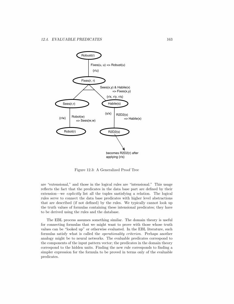
12.4. EVALUABLE PREDICATES 163
Robust(r)
Fixes(r, r)
Sees(r,r) Habile(s)
Robot(r) R2D2(s)
r/ws/x
r/x, r/y, r/s
r/u
Robot(w) => Sees(w,w)
R2D2(x) => Habile(x)
Sees(x,y) & Habile(x) => Fixes(x,y)
Fixes(u, u) => Robust(u)
becomes R2D2(r) afterapplying r/s
Figure 12.3: A Generalized Proof Tree
are “extensional,” and those in the logical rules are “intensional.” This usagereflects the fact that the predicates in the data base part are defined by theirextension—we explicitly list all the tuples sastisfying a relation. The logicalrules serve to connect the data base predicates with higher level abstractionsthat are described (if not defined) by the rules. We typically cannot look upthe truth values of formulas containing these intensional predicates; they haveto be derived using the rules and the database.
The EBL process assumes something similar. The domain theory is usefulfor connecting formulas that we might want to prove with those whose truthvalues can be “looked up” or otherwise evaluated. In the EBL literature, suchformulas satisfy what is called the operationality criterion. Perhaps anotheranalogy might be to neural networks. The evaluable predicates correspond tothe components of the input pattern vector; the predicates in the domain theorycorrespond to the hidden units. Finding the new rule corresponds to finding asimpler expression for the formula to be proved in terms only of the evaluablepredicates.

164 CHAPTER 12. EXPLANATION-BASED LEARNING
12.5 More General Proofs
Examining the domain theory for our example reveals that an alternative rulemight have been: Robot(u) ∧ C3PO(u) ⊃ Robust(u). Such a rule mighthave resulted if we were given C3PO(Num6), Robot(Num6), . . . and provedRobust(Num6). After considering these two examples (Num5 and Num6),the question arises, do we want to generalize the two rules to something like:Robot(u)∧ [C3PO(u)∨R2D2(u)] ⊃ Robust(u)? Doing so is an example of what[DeJong & Mooney, 1986] call structural generalization (via disjunctive augmen-tation ).
Adding disjunctions for every alternative proof can soon become cumbersomeand destroy any efficiency advantage of EBL. In our example, the efficiencymight be retrieved if there were another evaluable predicate, say, Bionic(u) suchthat the domain theory also contained R2D2(x) ⊃ Bionic(x) and C3PO(x) ⊃Bionic(x). After seeing a number of similar examples, we might be willing toinduce the formula Bionic(u) ⊃ [C3PO(u) ∨ R2D2(u)] in which case the rulewith the disjunction could be replaced with Robot(u)∧Bionic(u) ⊃ Robust(u).
12.6 Utility of EBL
It is well known in theorem proving that the complexity of finding a proofdepends both on the number of formulas in the domain theory and on the depthof the shortest proof. Adding a new rule decreases the depth of the shortestproof but it also increases the number of formulas in the domain theory. Inrealistic applications, the added rules will be relevant for some tasks and not forothers. Thus, it is unclear whether the overall utility of the new rules will turnout to be positive. EBL methods have been applied in several settings, usuallywith positive utility. (See [Minton, 1990] for an analysis).
12.7 Applications
There have been several applications of EBL methods. We mention two here,namely the formation of macro-operators in automatic plan generation andlearning how to control search.
12.7.1 Macro-Operators in Planning
In automatic planning systems, efficiency can sometimes be enhanced by chain-ing together a sequence of operators into macro-operators. We show an exam-ple of a process for creating macro-operators based on techniques explored by[Fikes, et al., 1972].
Referring to Fig. 12.4, consider the problem of finding a plan for a robot inroom R1 to fetch a box, B1, by going to an adjacent room, R2, and pushing it

12.7. APPLICATIONS 165
back to R1. The goal for the robot is INROOM(B1, R1), and the facts thatare true in the initial state are listed in the figure.
R1 R2
R3
D1
D2B1
Initial State:
INROOM(ROBOT, R1)INROOM(B1,R2)CONNECTS(D1,R1,R2)CONNECTS(D1,R2,R1)
. . .
Figure 12.4: Initial State of a Robot Problem
We will construct the plan from a set of STRIPS operators that include:
GOTHRU(d, r1, r2)
Preconditions: INROOM(ROBOT, r1), CONNECTS(d, r1, r2)
Delete list: INROOM(ROBOT, r1)
Add list: INROOM(ROBOT, r2)
PUSHTHRU(b, d, r1, r2)
Preconditions: INROOM(ROBOT, r1), CONNECTS(d, r1, r2), INROOM(b, r1)
Delete list: INROOM(ROBOT, r1), INROOM(b, r1)
Add list: INROOM(ROBOT, r2), INROOM(b, r2)
A backward-reasoning STRIPS system might produce the plan shown inFig. 12.5. We show there the main goal and the subgoals along a solution path.(The conditions in each subgoal that are true in the initial state are shownunderlined.) The preconditions for this plan, true in the initial state, are:
INROOM(ROBOT,R1)
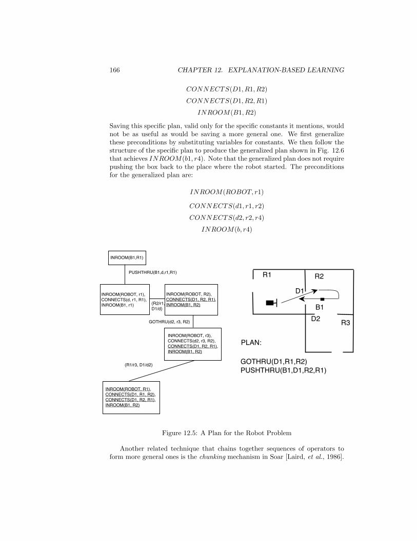
166 CHAPTER 12. EXPLANATION-BASED LEARNING
CONNECTS(D1, R1, R2)
CONNECTS(D1, R2, R1)
INROOM(B1, R2)
Saving this specific plan, valid only for the specific constants it mentions, wouldnot be as useful as would be saving a more general one. We first generalizethese preconditions by substituting variables for constants. We then follow thestructure of the specific plan to produce the generalized plan shown in Fig. 12.6that achieves INROOM(b1, r4). Note that the generalized plan does not requirepushing the box back to the place where the robot started. The preconditionsfor the generalized plan are:
INROOM(ROBOT, r1)
CONNECTS(d1, r1, r2)
CONNECTS(d2, r2, r4)
INROOM(b, r4)
INROOM(B1,R1)
PUSHTHRU(B1,d,r1,R1)
INROOM(ROBOT, r1),CONNECTS(d, r1, R1),INROOM(B1, r1)
INROOM(ROBOT, R2),CONNECTS(D1, R2, R1),INROOM(B1, R2)R2/r1,
D1/d
GOTHRU(d2, r3, R2)
INROOM(ROBOT, r3),CONNECTS(d2, r3, R2),CONNECTS(D1, R2, R1),INROOM(B1, R2)
R1/r3, D1/d2
INROOM(ROBOT, R1),CONNECTS(D1, R1, R2),CONNECTS(D1, R2, R1),INROOM(B1, R2)
R1 R2
R3
D1
D2
GOTHRU(D1,R1,R2)PUSHTHRU(B1,D1,R2,R1)
B1
PLAN:
Figure 12.5: A Plan for the Robot Problem
Another related technique that chains together sequences of operators toform more general ones is the chunking mechanism in Soar [Laird, et al., 1986].
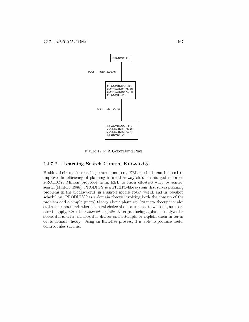
12.7. APPLICATIONS 167
INROOM(b1,r4)
PUSHTHRU(b1,d2,r2,r4)
INROOM(ROBOT, r2),CONNECTS(d1, r1, r2),CONNECTS(d2, r2, r4),INROOM(b1, r4)
GOTHRU(d1, r1, r2)
INROOM(ROBOT, r1),CONNECTS(d1, r1, r2),CONNECTS(d2, r2, r4),INROOM(b1, r4)
Figure 12.6: A Generalized Plan
12.7.2 Learning Search Control Knowledge
Besides their use in creating macro-operators, EBL methods can be used toimprove the efficiency of planning in another way also. In his system calledPRODIGY, Minton proposed using EBL to learn effective ways to controlsearch [Minton, 1988]. PRODIGY is a STRIPS-like system that solves planningproblems in the blocks-world, in a simple mobile robot world, and in job-shopscheduling. PRODIGY has a domain theory involving both the domain of theproblem and a simple (meta) theory about planning. Its meta theory includesstatements about whether a control choice about a subgoal to work on, an oper-ator to apply, etc. either succeeds or fails. After producing a plan, it analyzes itssuccessful and its unsuccessful choices and attempts to explain them in termsof its domain theory. Using an EBL-like process, it is able to produce usefulcontrol rules such as:

168 CHAPTER 12. EXPLANATION-BASED LEARNING
IF (AND (CURRENT− NODE node)
(CANDIDATE− GOAL node (ON x y))
(CANDIDATE− GOAL node (ON y z)))
THEN (PREFER GOAL (ON y z) TO (ON x y))
PRODIGY keeps statistics on how often these learned rules are used, theirsavings (in time to find plans), and their cost of application. It saves only therules whose utility, thus measured, is judged to be high. Minton [Minton, 1990]has shown that there is an overall advantage of using these rules (as against nothaving any rules and as against hand-coded search control rules).
12.8 Bibliographical and Historical RemarksTo be added.

Bibliography
[Acorn & Walden, 1992] Acorn, T., and Walden, S., “SMART: Support Man-agement Automated Reasoning Technology for COMPAQ Customer Ser-vice,” Proc. Fourth Annual Conf. on Innovative Applications of ArtificialIntelligence, Menlo Park, CA: AAAI Press, 1992.
[Aha, 1991] Aha, D., Kibler, D., and Albert, M., “Instance-Based LearningAlgorithms,” Machine Learning, 6, 37-66, 1991.
[Anderson & Bower, 1973] Anderson, J. R., and Bower, G. H., Human Asso-ciative Memory, Hillsdale, NJ: Erlbaum, 1973.
[Anderson, 1958] Anderson, T. W., An Introduction to Multivariate StatisticalAnalysis, New York: John Wiley, 1958.
[Barto, Bradtke, & Singh, 1994] Barto, A., Bradtke, S., and Singh, S., “Learn-ing to Act Using Real-Time Dynamic Programming,” to appear in Ar-tificial Intelligence, 1994.
[Baum & Haussler, 1989] Baum, E, and Haussler, D., “What Size Net GivesValid Generalization?” Neural Computation, 1, pp. 151-160, 1989.
[Baum, 1994] Baum, E., “When Are k-Nearest Neighbor and BackpropagationAccurate for Feasible-Sized Sets of Examples?” in Hanson, S., Drastal,G., and Rivest, R., (eds.), Computational Learning Theory and NaturalLearning Systems, Volume 1: Constraints and Prospects, pp. 415-442,Cambridge, MA: MIT Press, 1994.
[Bellman, 1957] Bellman, R. E., Dynamic Programming, Princeton: PrincetonUniversity Press, 1957.
[Blumer, et al., 1987] Blumer, A., et al., “Occam’s Razor,” Info. Process. Lett.,vol 24, pp. 377-80, 1987.
[Blumer, et al., 1990] Blumer, A., et al., “Learnability and the Vapnik-Chervonenkis Dimension,” JACM, 1990.
[Bollinger & Duffie, 1988] Bollinger, J., and Duffie, N., Computer Control ofMachines and Processes, Reading, MA: Addison-Wesley, 1988.
169
170 BIBLIOGRAPHY
[Brain, et al., 1962] Brain, A. E., et al., “Graphical Data Processing ResearchStudy and Experimental Investigation,” Report No. 8 (pp. 9-13) and No.9 (pp. 3-10), Contract DA 36-039 SC-78343, SRI International, MenloPark, CA, June 1962 and September 1962.
[Breiman, et al., 1984] Breiman, L., Friedman, J., Olshen, R., and Stone, C.,Classification and Regression Trees, Monterey, CA: Wadsworth, 1984.
[Brent, 1990] Brent, R. P., “Fast Training Algorithms for Multi-Layer NeuralNets,” Numerical Analysis Project Manuscript NA-90-03, Computer Sci-ence Department, Stanford University, Stanford, CA 94305, March 1990.
[Bryson & Ho 1969] Bryson, A., and Ho, Y.-C., Applied Optimal Control, NewYork: Blaisdell.
[Buchanan & Wilkins, 1993] Buchanan, B. and Wilkins, D., (eds.), Readings inKnowledge Acquisition and Learning, San Francisco: Morgan Kaufmann,1993.
[Carbonell, 1983] Carbonell, J., “Learning by Analogy,” in Machine Learning:An Artificial Intelligence Approach, Michalski, R., Carbonell, J., andMitchell, T., (eds.), San Francisco: Morgan Kaufmann, 1983.
[Cheeseman, et al., 1988] Cheeseman, P., et al., “AutoClass: A Bayesian Clas-sification System,” Proc. Fifth Intl. Workshop on Machine Learning,Morgan Kaufmann, San Mateo, CA, 1988. Reprinted in Shavlik, J. andDietterich, T., Readings in Machine Learning, Morgan Kaufmann, SanFrancisco, pp. 296-306, 1990.
[Cover & Hart, 1967] Cover, T., and Hart, P., “Nearest Neighbor Pattern Clas-sification,” IEEE Trans. on Information Theory, 13, 21-27, 1967.
[Cover, 1965] Cover, T., “Geometrical and Statistical Properties of Systemsof Linear Inequalities with Applications in Pattern Recognition,” IEEETrans. Elec. Comp., EC-14, 326-334, June, 1965.
[Dasarathy, 1991] Dasarathy, B. V., Nearest Neighbor Pattern ClassificationTechniques, IEEE Computer Society Press, 1991.
[Dayan & Sejnowski, 1994] Dayan, P., and Sejnowski, T., “TD(λ) Convergeswith Probability 1,” Machine Learning, 14, pp. 295-301, 1994.
[Dayan, 1992] Dayan, P., “The Convergence of TD(λ) for General λ,” MachineLearning, 8, 341-362, 1992.
[DeJong & Mooney, 1986] DeJong, G., and Mooney, R., “Explanation-BasedLearning: An Alternative View,” Machine Learning, 1:145-176, 1986.Reprinted in Shavlik, J. and Dietterich, T., Readings in Machine Learn-ing, San Francisco: Morgan Kaufmann, 1990, pp 452-467.
BIBLIOGRAPHY 171
[Dietterich & Bakiri, 1991] Dietterich, T. G., and Bakiri, G., “Error-CorrectingOutput Codes: A General Method for Improving Multiclass Induc-tive Learning Programs,” Proc. Ninth Nat. Conf. on A.I., pp. 572-577,AAAI-91, MIT Press, 1991.
[Dietterich, et al., 1990] Dietterich, T., Hild, H., and Bakiri, G., “A Compara-tive Study of ID3 and Backpropagation for English Text-to-Speech Map-ping,” Proc. Seventh Intl. Conf. Mach. Learning, Porter, B. and Mooney,R. (eds.), pp. 24-31, San Francisco: Morgan Kaufmann, 1990.
[Dietterich, 1990] Dietterich, T., “Machine Learning,” Annu. Rev. Comput.Sci., 4:255-306, Palo Alto: Annual Reviews Inc., 1990.
[Duda & Fossum, 1966] Duda, R. O., and Fossum, H., “Pattern Classificationby Iteratively Determined Linear and Piecewise Linear DiscriminantFunctions,” IEEE Trans. on Elect. Computers, vol. EC-15, pp. 220-232,April, 1966.
[Duda & Hart, 1973] Duda, R. O., and Hart, P.E., Pattern Classification andScene Analysis, New York: Wiley, 1973.
[Duda, 1966] Duda, R. O., “Training a Linear Machine on Mislabeled Patterns,”SRI Tech. Report prepared for ONR under Contract 3438(00), SRI In-ternational, Menlo Park, CA, April 1966.
[Efron, 1982] Efron, B., The Jackknife, the Bootstrap and Other ResamplingPlans, Philadelphia: SIAM, 1982.
[Ehrenfeucht, et al., 1988] Ehrenfeucht, A., et al., “A General Lower Bound onthe Number of Examples Needed for Learning,” in Proc. 1988 Workshopon Computational Learning Theory, pp. 110-120, San Francisco: MorganKaufmann, 1988.
[Etzioni, 1991] Etzioni, O., “STATIC: A Problem-Space Compiler forPRODIGY,” Proc. of Ninth National Conf. on Artificial Intelligence,pp. 533-540, Menlo Park: AAAI Press, 1991.
[Etzioni, 1993] Etzioni, O., “A Structural Theory of Explanation-Based Learn-ing,” Artificial Intelligence, 60:1, pp. 93-139, March, 1993.
[Evans & Fisher, 1992] Evans, B., and Fisher, D., Process Delay Analyses UsingDecision-Tree Induction, Tech. Report CS92-06, Department of Com-puter Science, Vanderbilt University, TN, 1992.
[Fahlman & Lebiere, 1990] Fahlman, S., and Lebiere, C., “The Cascade-Correlation Learning Architecture,” in Touretzky, D., (ed.), Advances inNeural Information Processing Systems, 2, pp. 524-532, San Francisco:Morgan Kaufmann, 1990.
172 BIBLIOGRAPHY
[Fayyad, et al., 1993] Fayyad, U. M., Weir, N., and Djorgovski, S., “SKICAT:A Machine Learning System for Automated Cataloging of Large ScaleSky Surveys,” in Proc. Tenth Intl. Conf. on Machine Learning, pp. 112-119, San Francisco: Morgan Kaufmann, 1993. (For a longer version ofthis paper see: Fayyad, U. Djorgovski, G., and Weir, N., “Automatingthe Analysis and Cataloging of Sky Surveys,” in Fayyad, U., et al.(eds.),Advances in Knowledge Discovery and Data Mining, Chapter 19, pp.471ff., Cambridge: The MIT Press, March, 1996.)
[Feigenbaum, 1961] Feigenbaum, E. A., “The Simulation of Verbal Learning Be-havior,” Proceedings of the Western Joint Computer Conference, 19:121-132, 1961.
[Fikes, et al., 1972] Fikes, R., Hart, P., and Nilsson, N., “Learning and Execut-ing Generalized Robot Plans,” Artificial Intelligence, pp 251-288, 1972.Reprinted in Shavlik, J. and Dietterich, T., Readings in Machine Learn-ing, San Francisco: Morgan Kaufmann, 1990, pp 468-486.
[Fisher, 1987] Fisher, D., “Knowledge Acquisition via Incremental ConceptualClustering,” Machine Learning, 2:139-172, 1987. Reprinted in Shavlik,J. and Dietterich, T., Readings in Machine Learning, San Francisco:Morgan Kaufmann, 1990, pp. 267–283.
[Friedman, et al., 1977] Friedman, J. H., Bentley, J. L., and Finkel, R. A., “AnAlgorithm for Finding Best Matches in Logarithmic Expected Time,”ACM Trans. on Math. Software, 3(3):209-226, September 1977.
[Fu, 1994] Fu, L., Neural Networks in Artificial Intelligence, New York:McGraw-Hill, 1994.
[Gallant, 1986] Gallant, S. I., “Optimal Linear Discriminants,” in Eighth Inter-national Conf. on Pattern Recognition, pp. 849-852, New York: IEEE,1986.
[Genesereth & Nilsson, 1987] Genesereth, M., and Nilsson, N., Logical Founda-tions of Artificial Intelligence, San Francisco: Morgan Kaufmann, 1987.
[Gluck & Rumelhart, 1989] Gluck, M. and Rumelhart, D., Neuroscience andConnectionist Theory, The Developments in Connectionist Theory, Hills-dale, NJ: Erlbaum Associates, 1989.
[Hammerstrom, 1993] Hammerstrom, D., “Neural Networks at Work,” IEEESpectrum, pp. 26-32, June 1993.
[Haussler, 1988] Haussler, D., “Quantifying Inductive Bias: AI Learning Al-gorithms and Valiant’s Learning Framework,” Artificial Intelligence,36:177-221, 1988. Reprinted in Shavlik, J. and Dietterich, T., Readings inMachine Learning, San Francisco: Morgan Kaufmann, 1990, pp. 96-107.
BIBLIOGRAPHY 173
[Haussler, 1990] Haussler, D., “Probably Approximately Correct Learning,”Proc. Eighth Nat. Conf. on AI, pp. 1101-1108. Cambridge, MA: MITPress, 1990.
[Hebb, 1949] Hebb, D. O., The Organization of Behaviour, New York: JohnWiley, 1949.
[Hertz, Krogh, & Palmer, 1991] Hertz, J., Krogh, A, and Palmer, R., Introduc-tion to the Theory of Neural Computation, Lecture Notes, vol. 1, SantaFe Inst. Studies in the Sciences of Complexity, New York: Addison-Wesley, 1991.
[Hirsh, 1994] Hirsh, H., “Generalizing Version Spaces,” Machine Learning, 17,5-45, 1994.
[Holland, 1975] Holland, J., Adaptation in Natural and Artificial Systems, AnnArbor: The University of Michigan Press, 1975. (Second edition printedin 1992 by MIT Press, Cambridge, MA.)
[Holland, 1986] Holland, J. H., “Escaping Brittleness; The Possibilities ofGeneral-Purpose Learning Algorithms Applied to Parallel Rule-BasedSystems.” In Michalski, R., Carbonell, J., and Mitchell, T. (eds.) , Ma-chine Learning: An Artificial Intelligence Approach, Volume 2, chapter20, San Francisco: Morgan Kaufmann, 1986.
[Hunt, Marin, & Stone, 1966] Hunt, E., Marin, J., and Stone, P., Experimentsin Induction, New York: Academic Press, 1966.
[Jabbour, K., et al., 1987] Jabbour, K., et al., “ALFA: Automated Load Fore-casting Assistant,” Proc. of the IEEE Pwer Engineering Society SummerMeeting, San Francisco, CA, 1987.
[John, 1995] John, G., “Robust Linear Discriminant Trees,” Proc. of the Conf.on Artificial Intelligence and Statistics, Ft. Lauderdale, FL, January,1995.
[Kaelbling, 1993] Kaelbling, L. P., Learning in Embedded Systems, Cambridge,MA: MIT Press, 1993.
[Kohavi, 1994] Kohavi, R., “Bottom-Up Induction of Oblivious Read-Once De-cision Graphs,” Proc. of European Conference on Machine Learning(ECML-94), 1994.
[Kolodner, 1993] Kolodner, J., Case-Based Reasoning, San Francisco: MorganKaufmann, 1993.
[Koza, 1992] Koza, J., Genetic Programming: On the Programming of Comput-ers by Means of Natural Selection, Cambridge, MA: MIT Press, 1992.
[Koza, 1994] Koza, J., Genetic Programming II: Automatic Discovery ofReusable Programs, Cambridge, MA: MIT Press, 1994.
174 BIBLIOGRAPHY
[Laird, et al., 1986] Laird, J., Rosenbloom, P., and Newell, A., “Chunking inSoar: The Anatomy of a General Learning Mechanism,” Machine Learn-ing, 1, pp. 11-46, 1986. Reprinted in Buchanan, B. and Wilkins, D.,(eds.), Readings in Knowledge Acquisition and Learning, pp. 518-535,Morgan Kaufmann, San Francisco, CA, 1993.
[Langley, 1992] Langley, P., “Areas of Application for Machine Learning,” Proc.of Fifth Int’l. Symp. on Knowledge Engineering, Sevilla, 1992.
[Langley, 1996] Langley, P., Elements of Machine Learning, San Francisco:Morgan Kaufmann, 1996.
[Lavrac & Dzeroski, 1994] Lavrac, N., and Dzeroski, S., Inductive Logic Pro-gramming, Chichester, England: Ellis Horwood, 1994.
[Lin, 1992] Lin, L., “Self-Improving Reactive Agents Based on ReinforcementLearning, Planning, and Teaching,” Machine Learning, 8, 293-321, 1992.
[Lin, 1993] Lin, L., “Scaling Up Reinforcement Learning for Robot Control,”Proc. Tenth Intl. Conf. on Machine Learning, pp. 182-189, San Francisco:Morgan Kaufmann, 1993.
[Littlestone, 1988] Littlestone, N., “Learning Quickly When Irrelevant At-tributes Abound: A New Linear-Threshold Algorithm,” Machine Learn-ing 2: 285-318, 1988.
[Maass & Turan, 1994] Maass, W., and Turan, G., “How Fast Can a Thresh-old Gate Learn?,” in Hanson, S., Drastal, G., and Rivest, R., (eds.),Computational Learning Theory and Natural Learning Systems, Volume1: Constraints and Prospects, pp. 381-414, Cambridge, MA: MIT Press,1994.
[Mahadevan & Connell, 1992] Mahadevan, S., and Connell, J., “AutomaticProgramming of Behavior-Based Robots Using Reinforcement Learn-ing,” Artificial Intelligence, 55, pp. 311-365, 1992.
[Marchand & Golea, 1993] Marchand, M., and Golea, M., “On Learning Sim-ple Neural Concepts: From Halfspace Intersections to Neural DecisionLists,” Network, 4:67-85, 1993.
[McCulloch & Pitts, 1943] McCulloch, W. S., and Pitts, W. H., “A Logical Cal-culus of the Ideas Immanent in Nervous Activity,” Bulletin of Mathe-matical Biophysics, Vol. 5, pp. 115-133, Chicago: University of ChicagoPress, 1943.
[Michie, 1992] Michie, D., “Some Directions in Machine Intelligence,” unpub-lished manuscript, The Turing Institute, Glasgow, Scotland, 1992.
[Minton, 1988] Minton, S., Learning Search Control Knowledge: AnExplanation-Based Approach, Kluwer Academic Publishers, Boston,MA, 1988.
BIBLIOGRAPHY 175
[Minton, 1990] Minton, S., “Quantitative Results Concerning the Utility ofExplanation-Based Learning,” Artificial Intelligence, 42, pp. 363-392,1990. Reprinted in Shavlik, J. and Dietterich, T., Readings in MachineLearning, San Francisco: Morgan Kaufmann, 1990, pp. 573-587.
[Mitchell, et al., 1986] Mitchell, T., et al., “Explanation-Based Generalization:A Unifying View,” Machine Learning, 1:1, 1986. Reprinted in Shavlik,J. and Dietterich, T., Readings in Machine Learning, San Francisco:Morgan Kaufmann, 1990, pp. 435-451.
[Mitchell, 1982] Mitchell, T., “Generalization as Search,” Artificial Intelligence,18:203-226, 1982. Reprinted in Shavlik, J. and Dietterich, T., Readings inMachine Learning, San Francisco: Morgan Kaufmann, 1990, pp. 96–107.
[Moore & Atkeson, 1993] Moore, A., and Atkeson, C., “Prioritized Sweeping:Reinforcement Learning with Less Data and Less Time,” Machine Learn-ing, 13, pp. 103-130, 1993.
[Moore, et al., 1994] Moore, A. W., Hill, D. J., and Johnson, M. P., “An Em-pirical Investigation of Brute Force to Choose Features, Smoothers, andFunction Approximators,” in Hanson, S., Judd, S., and Petsche, T.,(eds.), Computational Learning Theory and Natural Learning Systems,Vol. 3, Cambridge: MIT Press, 1994.
[Moore, 1990] Moore, A., Efficient Memory-based Learning for Robot Control,PhD. Thesis; Technical Report No. 209, Computer Laboratory, Univer-sity of Cambridge, October, 1990.
[Moore, 1992] Moore, A., “Fast, Robust Adaptive Control by Learning OnlyForward Models,” in Moody, J., Hanson, S., and Lippman, R., (eds.),Advances in Neural Information Processing Systems 4, San Francisco:Morgan Kaufmann, 1992.
[Mueller & Page, 1988] Mueller, R. and Page, R., Symbolic Computing withLisp and Prolog, New York: John Wiley & Sons, 1988.
[Muggleton, 1991] Muggleton, S., “Inductive Logic Programming,” New Gen-eration Computing, 8, pp. 295-318, 1991.
[Muggleton, 1992] Muggleton, S., Inductive Logic Programming, London: Aca-demic Press, 1992.
[Muroga, 1971] Muroga, S., Threshold Logic and its Applications, New York:Wiley, 1971.
[Natarjan, 1991] Natarajan, B., Machine Learning: A Theoretical Approach,San Francisco: Morgan Kaufmann, 1991.
176 BIBLIOGRAPHY
[Nilsson, 1965] Nilsson, N. J., “Theoretical and Experimental Investigations inTrainable Pattern-Classifying Systems,” Tech. Report No. RADC-TR-65-257, Final Report on Contract AF30(602)-3448, Rome Air Develop-ment Center (Now Rome Laboratories), Griffiss Air Force Base, NewYork, September, 1965.
[Nilsson, 1990] Nilsson, N. J., The Mathematical Foundations of Learning Ma-chines, San Francisco: Morgan Kaufmann, 1990. (This book is a reprintof Learning Machines: Foundations of Trainable Pattern-ClassifyingSystems, New York: McGraw-Hill, 1965.)
[Oliver, Dowe, & Wallace, 1992] Oliver, J., Dowe, D., and Wallace, C., “Infer-ring Decision Graphs using the Minimum Message Length Principle,”Proc. 1992 Australian Artificial Intelligence Conference, 1992.
[Pagallo & Haussler, 1990] Pagallo, G. and Haussler, D., “Boolean Feature Dis-covery in Empirical Learning,” Machine Learning, vol.5, no.1, pp. 71-99,March 1990.
[Pazzani & Kibler, 1992] Pazzani, M., and Kibler, D., “The Utility of Knowl-edge in Inductive Learning,” Machine Learning, 9, 57-94, 1992.
[Peterson, 1961] Peterson, W., Error Correcting Codes, New York: John Wiley,1961.
[Pomerleau, 1991] Pomerleau, D., “Rapidly Adapting Artificial Neural Net-works for Autonomous Navigation,” in Lippmann, P., et al. (eds.), Ad-vances in Neural Information Processing Systems, 3, pp. 429-435, SanFrancisco: Morgan Kaufmann, 1991.
[Pomerleau, 1993] Pomerleau, D, Neural Network Perception for Mobile RobotGuidance, Boston: Kluwer Academic Publishers, 1993.
[Quinlan & Rivest, 1989] Quinlan, J. Ross, and Rivest, Ron, “Inferring Deci-sion Trees Using the Minimum Description Length Principle,” Informa-tion and Computation, 80:227–248, March, 1989.
[Quinlan, 1986] Quinlan, J. Ross, “Induction of Decision Trees,” MachineLearning, 1:81–106, 1986. Reprinted in Shavlik, J. and Dietterich, T.,Readings in Machine Learning, San Francisco: Morgan Kaufmann, 1990,pp. 57–69.
[Quinlan, 1987] Quinlan, J. R., “Generating Production Rules from DecisionTrees,” In IJCAI-87: Proceedings of the Tenth Intl. Joint Conf. on Ar-tificial Intelligence, pp. 304-7, San Francisco: Morgan-Kaufmann, 1987.
[Quinlan, 1990] Quinlan, J. R., “Learning Logical Definitions from Relations,”Machine Learning, 5, 239-266, 1990.
BIBLIOGRAPHY 177
[Quinlan, 1993] Quinlan, J. Ross, C4.5: Programs for Machine Learning, SanFrancisco: Morgan Kaufmann, 1993.
[Quinlan, 1994] Quinlan, J. R., “Comparing Connectionist and Symbolic Learn-ing Methods,” in Hanson, S., Drastal, G., and Rivest, R., (eds.), Com-putational Learning Theory and Natural Learning Systems, Volume 1:Constraints and Prospects, pp. 445-456,, Cambridge, MA: MIT Press,1994.
[Ridgway, 1962] Ridgway, W. C., An Adaptive Logic System with GeneralizingProperties, PhD thesis, Tech. Rep. 1556-1, Stanford Electronics Labs.,Stanford, CA, April 1962.
[Rissanen, 1978] Rissanen, J., “Modeling by Shortest Data Description,” Auto-matica, 14:465-471, 1978.
[Rivest, 1987] Rivest, R. L., “Learning Decision Lists,” Machine Learning, 2,229-246, 1987.
[Rosenblatt, 1958] Rosenblatt, F., Principles of Neurodynamics, Washington:Spartan Books, 1961.
[Ross, 1983] Ross, S., Introduction to Stochastic Dynamic Programming, NewYork: Academic Press, 1983.
[Rumelhart, Hinton, & Williams, 1986] Rumelhart, D. E., Hinton, G. E., andWilliams, R. J., “Learning Internal Representations by Error Propa-gation,” In Rumelhart, D. E., and McClelland, J. L., (eds.) ParallelDistributed Processing, Vol 1, 318–362, 1986.
[Russell & Norvig 1995] Russell, S., and Norvig, P., Artificial Intelligence: AModern Approach, Englewood Cliffs, NJ: Prentice Hall, 1995.
[Samuel, 1959] Samuel, A., “Some Studies in Machine Learning Using the Gameof Checkers,” IBM Journal of Research and Development, 3:211-229, July1959.
[Schwartz, 1993] Schwartz, A., “A Reinforcement Learning Method for Max-imizing Undiscounted Rewards,” Proc. Tenth Intl. Conf. on MachineLearning, pp. 298-305, San Francisco: Morgan Kaufmann, 1993.
[Sejnowski, Koch, & Churchland, 1988] Sejnowski, T., Koch, C., and Church-land, P., “Computational Neuroscience,” Science, 241: 1299-1306, 1988.
[Shavlik, Mooney, & Towell, 1991] Shavlik, J., Mooney, R., and Towell, G.,“Symbolic and Neural Learning Algorithms: An Experimental Compar-ison,” Machine Learning, 6, pp. 111-143, 1991.
[Shavlik & Dietterich, 1990] Shavlik, J. and Dietterich, T., Readings in Ma-chine Learning, San Francisco: Morgan Kaufmann, 1990.
178 BIBLIOGRAPHY
[Sutton & Barto, 1987] Sutton, R. S., and Barto, A. G., “A Temporal-Difference Model of Classical Conditioning,” in Proceedings of the NinthAnnual Conference of the Cognitive Science Society, Hillsdale, NJ: Erl-baum, 1987.
[Sutton, 1988] Sutton, R. S., “Learning to Predict by the Methods of TemporalDifferences,” Machine Learning 3: 9-44, 1988.
[Sutton, 1990] Sutton, R., “Integrated Architectures for Learning, Planning,and Reacting Based on Approximating Dynamic Programming,” Proc. ofthe Seventh Intl. Conf. on Machine Learning, pp. 216-224, San Francisco:Morgan Kaufmann, 1990.
[Taylor, Michie, & Spiegalhalter, 1994] Taylor, C., Michie, D., and Spiegal-halter, D., Machine Learning, Neural and Statistical Classification,Paramount Publishing International.
[Tesauro, 1992] Tesauro, G., “Practical Issues in Temporal Difference Learn-ing,” Machine Learning, 8, nos. 3/4, pp. 257-277, 1992.
[Towell & Shavlik, 1992] Towell G., and Shavlik, J., “Interpretation of Artifi-cial Neural Networks: Mapping Knowledge-Based Neural Networks intoRules,” in Moody, J., Hanson, S., and Lippmann, R., (eds.), Advances inNeural Information Processing Systems, 4, pp. 977-984, San Francisco:Morgan Kaufmann, 1992.
[Towell, Shavlik, & Noordweier, 1990] Towell, G., Shavlik, J., and Noordweier,M., “Refinement of Approximate Domain Theories by Knowledge-BasedArtificial Neural Networks,” Proc. Eighth Natl., Conf. on Artificial In-telligence, pp. 861-866, 1990.
[Unger, 1989] Unger, S., The Essence of Logic Circuits, Englewood Cliffs, NJ:Prentice-Hall, 1989.
[Utgoff, 1989] Utgoff, P., “Incremental Induction of Decision Trees,” MachineLearning, 4:161–186, Nov., 1989.
[Valiant, 1984] Valiant, L., “A Theory of the Learnable,” Communications ofthe ACM, Vol. 27, pp. 1134-1142, 1984.
[Vapnik & Chervonenkis, 1971] Vapnik, V., and Chervonenkis, A., “On theUniform Convergence of Relative Frequencies, Theory of Probability andits Applications, Vol. 16, No. 2, pp. 264-280, 1971.
[Various Editors, 1989-1994] Advances in Neural Information Processing Sys-tems, vols 1 through 6, San Francisco: Morgan Kaufmann, 1989 -1994.
[Watkins & Dayan, 1992] Watkins, C. J. C. H., and Dayan, P., “Technical Note:Q-Learning,” Machine Learning, 8, 279-292, 1992.
BIBLIOGRAPHY 179
[Watkins, 1989] Watkins, C. J. C. H., Learning From Delayed Rewards, PhDThesis, University of Cambridge, England, 1989.
[Weiss & Kulikowski, 1991] Weiss, S., and Kulikowski, C., Computer Systemsthat Learn, San Francisco: Morgan Kaufmann, 1991.
[Werbos, 1974] Werbos, P., Beyond Regression: New Tools for Prediction andAnalysis in the Behavioral Sciences, Ph.D. Thesis, Harvard University,1974.
[Widrow & Lehr, 1990] Widrow, B., and Lehr, M. A., “30 Years of AdaptiveNeural Networks: Perceptron, Madaline and Backpropagation,” Proc.IEEE, vol. 78, no. 9, pp. 1415-1442, September, 1990.
[Widrow & Stearns, 1985] Widrow, B., and Stearns, S., Adaptive Signal Pro-cessing, Englewood Cliffs, NJ: Prentice-Hall.
[Widrow, 1962] Widrow, B., “Generalization and Storage in Networks of Ada-line Neurons,” in Yovits, Jacobi, and Goldstein (eds.), Self-organizingSystems—1962, pp. 435-461, Washington, DC: Spartan Books, 1962.
[Winder, 1961] Winder, R., “Single Stage Threshold Logic,” Proc. of the AIEESymp. on Switching Circuits and Logical Design, Conf. paper CP-60-1261, pp. 321-332, 1961.
[Winder, 1962] Winder, R., Threshold Logic, PhD Dissertation, Princeton Uni-versity, Princeton, NJ, 1962.
[Wnek, et al., 1990] Wnek, J., et al., “Comparing Learning Paradigms via Di-agrammatic Visualization,” in Proc. Fifth Intl. Symp. on Methodologiesfor Intelligent Systems, pp. 428-437, 1990. (Also Tech. Report MLI90-2,University of Illinois at Urbana-Champaign.)


![Introduction to Key Machine Learning Technologies · Introduction to Key Machine Learning Technologies Ken Shioiri [Summary] Machine learning, typically represented by Deep Learning,](https://img.pdfslide.us/doc/110x75/5ec740f61231d239d701eac1/introduction-to-key-machine-learning-technologies-introduction-to-key-machine-learning.jpg)