Faculté des géosciences et de l’environnementCentre de recherche en environnement terrestre Dynamic Modelling of Material Flows and Sustainable Resource Use Case Studies in Regional Metabolism and Space Life Support SystemsThèse de doctoratprésentée à la Faculté des géosciences et de l’environnement de l’Université de Lausanne, Suisse, parEmilia Suomalainen

Master of Science in Technology, Helsinki University of Technology, Finlandepour l’obtention du grade de Doctorat en géosciences et environnement, mention Sciences de l’environnement

Composition du jury:Prof. Jean-Luc Epard Président du jury ISTE, FGSE, UNILProf. Suren Erkman Directeur de thèse CRET, FGSE, UNILProf. Torsten Vennemann Expert interne ISTE, FGSE, UNILProf. Ugo Bardi Expert externe Dipartimento di Chimica "Ugo Schiff", Università di FirenzeDr. Christophe Lasseur Expert externe ESTEC, European Space Agency

Lausanne, 2012

Faculté des géosciences et de l’environnementCentre de recherche en environnement terrestre Dynamic Modelling of Material Flows and Sustainable Resource Use Case Studies in Regional Metabolism and Space Life Support SystemsThèse de doctoratprésentée à la Faculté des géosciences et de l’environnement de l’Université de Lausanne, Suisse, parEmilia Suomalainen

Master of Science in Technology, Helsinki University of Technology, Finlandepour l’obtention du grade de Doctorat en géosciences et environnement, mention Sciences de l’environnement

Composition du jury:Prof. Jean-Luc Epard Président du jury ISTE, FGSE, UNILProf. Suren Erkman Directeur de thèse CRET, FGSE, UNILProf. Torsten Vennemann Expert interne ISTE, FGSE, UNILProf. Ugo Bardi Expert externe Dipartimento di Chimica "Ugo Schiff", Università di FirenzeDr. Christophe Lasseur Expert externe ESTEC, European Space Agency

Lausanne, 2012

iv

AbstractSustainable resource use is one of the most important environmental issues of our times. It is closely related to the discussions on the ‘peaking’ of various natural resources serving as energy sources, agricultural nutrients, or metals indispensable in high-technology applications. Although the peaking concept remains controversial, it is commonly recognized that a more resource management would help to alleviate negative environmental impacts related to resource use. In this thesis, sustainable resource use is analysed from a practical standpoint, through several different case studies. Four of these case studies relate to resource metabolism in the Canton of Geneva in Switzerland: the aim was to model the evolution of chosen resource stocks and flows in the coming decades. The studied resources were copper (a bulk metal), phosphorus (a vital agricultural nutrient), and wood (a renewable resource). In addition, the case of lithium (a critical metal) was analysed briefly in a qualitative manner and in an electric mobility perspective. In addition to the Geneva case studies, this thesis includes a case study on the sustainability of space life support systems. Space life support systems are systems whose aim is to provide the crew of a spacecraft with the necessary metabolic consumables over the course of a mission. Sustainability was again analysed from a resource use perspective. In this case study, the functioning of two different types of life support systems, ARES and BIORAT, was evaluated and compared; these systems represent, respectively, a physico-chemical and biological life support system. Space life support systems could in fact be used as a kind of ‘sustainability laboratory’ given that they represent closed and relatively simple systems compared to complex and open terrestrial systems such as the Canton of Geneva. The chosen analysis method used in the Geneva case studies was dynamic material flow analysis: dynamic material flow models were constructed for the resources copper, phosphorus, and wood. Besides a baseline scenario, various alternative scenarios (notably involving increased recycling) were examined. In the case of space life support systems, the methodology of material flow analysis was also employed, but as the data available on the dynamic behaviour of the systems was insufficient, only static simulations could be performed. The results of the case studies in the Canton of Geneva show the following: were resource use to follow population growth, resource consumption would be multiplied by nearly 1.2 by 2030 and by 1.5 by 2080. A complete transition to electric mobility would be expected to increase the copper consumption per capita only slightly (+5%) while the lithium demand in cars would increase 350 fold. Phosphorus imports could be decreased by recycling sewage sludge or human urine; however, the health and environmental impacts of these options are yet to be studied. Increasing the wood production in the v

Canton would not significantly decrease the dependence on wood imports as the Canton’s production represents only 5% of the total consumption. In the comparison of space life support systems ARES and BIORAT, BIORAT outperforms ARES in resource use but not in energy use. However, as the systems are dimensioned very differently, it remains debatable whether they can be compared outright. In conclusion, the use of dynamic material flow analysis can provide useful information for policy makers and strategic decision-making; however, uncertainty in reference data greatly influences the precision of the results. Space life support systems constitute an extreme case of resource-using systems; nevertheless, it is not clear how their example could be of immediate use to terrestrial systems.

vi

RésuméL’utilisation durable des ressources fait partie des grandes problématiques environnementales. Elle est étroitement liée aux discussions sur le ‘pic’ de production des ressources naturelles comme les sources d’énergie, les nutriments agricoles ou les métaux indispensables dans des applications de haute technologie. Bien que ce concept reste controversé, il est généralement admis que l’utilisation plus durable des ressources naturelles permettrait d'atténuer les impacts environnementaux indésirables liés à leur utilisation.Dans cette thèse de doctorat, l’utilisation durable des ressources fat l’objet d’une analyse appliquée au travers de divers études de cas. Quatre de ces études de cas concernent le métabolisme des ressources dans le canton de Genève en Suisse, le but étant de modéliser l’évolution des stocks et des flux de certaines ressources données pendant les prochaines décennies. Les ressources étudiées incluent le cuivre (un métal critique), le phosphore (un fertilisant agricole) et le bois (une ressource renouvelable). De plus, le cas du lithium est analysé brièvement d’une manière qualitative dans un contexte de mobilité électrique.En plus des études de cas genevoises, ce travail de thèse inclut une étude sur la durabilité des systèmes de support vie spatiaux. Les systèmes de support vie spatiaux sont des systèmes qui fournissent de l’oxygène, de l’eau et de la nourriture à l’équipage d’une navette spatiale pendant la mission. La durabilité de ces systèmes est analysée du point de vue de l’utilisation des ressources dans le but d’évaluer et de comparer le fonctionnement de deux systèmes de support vie, ARES et BIORAT. Ces systèmes représentent respectivement un système de support vie chimico-technique et biologique. Les systèmes de support vie pourraient en effet être utilisés comme « laboratoire de durabilité » puisqu’ils représentent des systèmes clos et relativement simples comparés aux systèmes terrestres ouverts et complexes, comme le canton de Genève. La méthode d’analyse appliquée aux études de cas genevoises était l’analyse de flux de matériaux dynamique. Des modèles de flux de matériaux dynamiques ont étés construits pour les ressources cuivre, phosphore et bois. En plus d’un scénario tendanciel, des différents scénarios alternatifs (concernant notamment un taux de recyclage plus élevé) ont également été définis. Dans le cas des systèmes de support vie, l’analyse de flux de matériaux était également utilisée mais à cause de la manque d’information seulement des simulations statiques ont étés réalisées.Les résultats des études de cas à Genève indiquent que si la consommation évolue suivant la croissance de la population (scénario tendanciel), l’utilisation des ressources sera multipliée par presque 1,2 en 2030 et par 1,5 en 2080. Une transition complète vers la mobilité électrique n’aurait pas de grande influence sur l’utilisation du cuivre (une augmentation de 5 %) ; par contre, la quantité de lithium dans vii

le stock de voitures serait multipliée par 350. Les importations de phosphore pourraient être diminuées grâce au recyclage des boues d’épuration ou de l’urine humaine mais les impacts sur la santé et l’environnement doivent encore être étudiés. L’augmentation de la production du bois dans le canton ne permettrait pas de diminuer la dépendance sur les importations d’une manière significative puisque la production cantonale ne représente que 5 % de la consommation totale du bois. En ce qui concerne les systèmes de support vie ARES et BIORAT, BIORAT surpasse ARES en utilisation durable des ressources mais il consomme dix fois plus d’énergie. En fin de compte, ces deux systèmes ont des tailles tellement différentes qu’il n’est pas clair s’il peuvent être comparés directement. En conclusion, la méthodologie de l’analyse de flux de matériaux dynamique peut apporter des informations utiles pour les politiques publiques et la prise de décision stratégique ; cependant l’incertitude dans les données de départ a une grande influence sur les résultats de la modélisation. Les systèmes de support de vie spatiaux constituent un cas extrême de systèmes clos ; toutefois il n’est pas évident comment leur exemple pourrait être d’une utilité immédiate aux systèmes terrestres.

viii

AcknowledgementsIn chronological order, I would like to begin by thanking Bertrand Guillaume from the University of Technology of Troyes for putting me in contact with Professor Erkman when I was looking for a project. The case study on space life support systems was part of an European Space Agency project, ALiSSE Phase 2, on the evaluation of space life support systems. I would like to thank ESA and in particular Christophe Lasseur for including the sustainability aspect in the scope of the project and for providing financing for my thesis. In addition, I thank Jean Brunet and Olivier Gerbi from Sherpa Engineering, the main contractor of the ALiSSE project, who provided me with assistance, documentation, and advice on the systemic aspects. I also offer my thanks to Christophe Blavot who gave me a job at Écologie Industrielle Conseil when I needed one. The case studies in the Canton of Geneva were financed by the Canton in the broader framework of the Ecosite project. I am extremely grateful for this opportunity and I would like to thank in particular Mr Daniel Chambaz, Director of the Geneva Environmental Office. I am also grateful to Laetitia Carles for taking on the difficult task of presenting my work when I was unable to do so myself. I thank all my numerous ex-colleagues and various visitors at IPTEH for their insightful comments as well as for creating an extremely stimulating and fun working environment. A special thanks goes to Tourane Corbière-Nicollier for reading and commenting my first Geneva case study. I offer my greatest thanks to Professor Suren Erkman who offered me this thesis project, helped to arrange its financing, and provided me with invaluable counsel and guidance during these four years. Lastly, I thank Olivier for his unfailing support that has helped me through this project.

ix

x

Table of Contents

PART I: INTRODUCTION AND THEORY_____________________________________________________________________19

Chapter 1 Introduction_______________________________________________________________________________________211.1 Background______________________________________________________________________________________________211.2 Objectives and Scope___________________________________________________________________________________221.3 Methods and Tools______________________________________________________________________________________231.4 Context___________________________________________________________________________________________________251.5 Case Studies ____________________________________________________________________________________________271.6 Contents_________________________________________________________________________________________________281.7 Terminology_____________________________________________________________________________________________31Chapter 2 Resource Use and Scarcity______________________________________________________________________332.1 Basic Concepts and Definitions________________________________________________________________________332.2 Resource Depletion and Scarcity ______________________________________________________________________392.3 Resource Use and Sustainability_______________________________________________________________________442.4 Indicators of Sustainable Resource Use _______________________________________________________________482.5 Conclusion_______________________________________________________________________________________________52PART II: MODEL FRAMEWORK______________________________________________________________________________55

Chapter 3 Modelling Resource Use_________________________________________________________________________573.1 Introduction to Models_________________________________________________________________________________573.2 Dynamic MFA Models___________________________________________________________________________________653.3 Dynamic MFA Model Framework______________________________________________________________________683.4 Uncertainty Assessment________________________________________________________________________________773.5 Discussion_______________________________________________________________________________________________833.6 Conclusion_______________________________________________________________________________________________85PART III: CASE STUDIES AND MODEL CONSTRUCTION__________________________________________________87

Chapter 4 Case Study on Copper ___________________________________________________________________________894.1 Introduction_____________________________________________________________________________________________894.2 Dynamic Modelling of Copper Metabolism in the Canton of Geneva________________________________924.3 Evolution of Copper World Production______________________________________________________________1124.4 Autarky_________________________________________________________________________________________________1184.5 Discussion______________________________________________________________________________________________1224.6 Conclusion_____________________________________________________________________________________________123Chapter 5 Case Study on Phosphorus____________________________________________________________________1255.1 Introduction____________________________________________________________________________________________125

xi

5.2 Phosphorus Metabolism in Switzerland_____________________________________________________________1305.3 Phosphorus Metabolism in the Canton of Geneva___________________________________________________1365.4 Dynamic Modelling of Phosphorus Metabolism_____________________________________________________1465.5 Uncertainty Analysis__________________________________________________________________________________1555.6 Discussion & Conclusion______________________________________________________________________________158Chapter 6 Case Study on Wood____________________________________________________________________________1616.1 Introduction____________________________________________________________________________________________1616.2 Wood Metabolism in the Canton of Geneva__________________________________________________________1626.3 Dynamic Modelling of Wood Metabolism____________________________________________________________1646.4 Discussion & Conclusion______________________________________________________________________________176Chapter 7 Case Study on Lithium__________________________________________________________________________1797.1 Introduction____________________________________________________________________________________________1797.2 Lithium and the Canton of Geneva___________________________________________________________________1817.3 Discussion & Conclusion______________________________________________________________________________183Chapter 8 Case Study on Space Life Support Systems__________________________________________________1858.1 Introduction____________________________________________________________________________________________1858.2 Modelling the Sustainability of Space Life Support Systems_______________________________________1908.3 Discussion & Conclusion______________________________________________________________________________214PART IV: RECOMMENDATIONS AND CONCLUSION______________________________________________________217

Chapter 9 Policy for Sustainable Resource Management______________________________________________2199.1 Introduction____________________________________________________________________________________________2199.2 Resource Use Strategies_______________________________________________________________________________2209.3 On Resource Policy and Leverage Points_____________________________________________________________2289.4 On the Use of the Dynamic MFA Model in Policy Analysis__________________________________________2319.5 Conclusion_____________________________________________________________________________________________232Chapter 10 Recommendations & Conclusion___________________________________________________________23310.1 Introduction__________________________________________________________________________________________23310.2 Resource-Specific Recommendations ______________________________________________________________23410.3 General Recommendations__________________________________________________________________________23710.4 Lessons Learned from Space Life Support Systems_______________________________________________23910.5 Conclusion____________________________________________________________________________________________240Table of Contents____________________________________________________________________________________________249

List of Figures________________________________________________________________________________________________257

List of Tables_________________________________________________________________________________________________261

References____________________________________________________________________________________________________263xii

APPENDICES__________________________________________________________________________________________________283

Appendix A Hubbert’s Peak Model_______________________________________________________________________285

Appendix B Case Study on Copper________________________________________________________________________287

Appendix C Case Study on Phosphorus__________________________________________________________________313

Appendix D Case Study on Wood__________________________________________________________________________329

Appendix E Case Study on Space Life Support Systems________________________________________________335

Appendix F Recommendations____________________________________________________________________________347

xiii

xiv

AbbreviationsALiSSE Advanced Life Support System EvaluatorARES Air REvitalization System; a physico-chemical air revitalization system developed by AstriumBaU Business as UsualBIORAT A biological air revitalization system developed by ESAC Symbol of the chemical element carbonCO2 Carbon dioxide in its molecular formCu Symbol of the chemical element copperE-mobility Electric mobilityESA European Space AgencyESM Equivalent System MassEV Electric VehicleFOEN Swiss Federal Office for the EnvironmentFSO Swiss Federal Statistical OfficeGt Gigatonne, 109 metric tonsH Symbol of the chemical element hydrogenICE Internal Combustion EngineIRM Integrated Resource ManagementLCA Life Cycle Analysis or Life Cycle AssessmentLi Symbol of the chemical element lithiumLSS Life Support SystemMBM Meat and Bone MealMELiSSA Micro-Ecological Life Support System AlternativeMFA Material Flow AnalysisMt Megatonne, 106 metric tonsxv

N Symbol of the chemical element nitrogenO Symbol of the chemical element oxygenO2 Oxygen in its molecular formOCSTAT Statistical Office of the Canton of GenevaP Symbol of the chemical element phosphorusPBR PhotobioreactorS Symbol of the chemical element sulphurSFA Substance Flow AnalysisSMM Sustainable Materials Managementt Metric tonUNEP United Nations Environment ProgrammeUSGS United States Geological Survey

xvi

‘Essentially, all models are wrong, but some are useful.’George E.P. Box, Empirical Model-Building and Response Surfaces (1987), co-authored with Norman R. Draper, p. 424‘On two occasions I have been asked, “Pray, Mr. Babbage, if you put into the machine wrong figures, will the right answers come out?” ... I am not able rightly to apprehend the kind of confusion of ideas that could provoke such a question.’ Charles Babbage, Passages from the Life of a Philosopher (1864), p. 67‘It is exceedingly difficult to make predictions, particularly about the future.’ Attributed to Niels Bohr (1885-1962)

xvii

Thesis Structure

PART IINTRODUCTION AND THEORY

20

Chapter 1: IntroductionChapter 1 Introduction1.1 BackgroundSustainable resource use is a topic that has been under much discussion in recent years notably in various scarcity- and peak-related debates concerning, for instance fossil fuels (such as oil and gas), various other energy sources (e.g. uranium), agricultural nutrients (notably phosphorus), various critical and strategic metals (for instance lithium, rhodium, indium, and gallium) as well as rare earth metals. However, resource depletion and scarcity remain controversial issues dividing growth optimists, who are often attached to an economic view of resource scarcity, and growth pessimists advocating physical limits. The controversy is not new, dating back to the famous The Limits to Growth report of 1972. One could argue that the debate is even older, stemming from the original Malthusian population models formulated at the turn of the 18th century. The theory on the peak of production of non-renewable resources has also been around for a long time: it was first formulated by M. King Hubbert in the 1950s. Resource depletion and scarcity are closely related to the concept of sustainable resource use which constitutes the main topic of this thesis. And although the questions of scarcity and resource depletion remain controversial, sustainable resource use has, somewhat surprisingly, become an important and generally accepted concept. This stems perhaps from the fact that scarcity concerns and the environmental impacts of resource use are closely linked and that sustainable resource use would help to alleviate both these problems. Environmental impacts of resource use cover a wide range of issues from eutrophication and soil erosion to loss of biodiversity and global warming. Or perhaps it is the fact that the term ‘resource use’ is proceeded by the nowadays nearly vacuous ‘sustainable’ buzzword that renders the concept of sustainable resource use acceptable and provides it with an aura of respectability. However, there is no clear definition of what sustainable resource use actually is or what level of resource use can be qualified as sustainable. The 6th Environment Action Programme of the European Union states (somewhat vaguely) that achieving sustainable resource use requires ‘ensur[ing] that the consumption of renewable and non-renewable resources and the associated impacts do not exceed the carrying capacity of the environment’ and ‘achiev[ing] a decoupling of resource use from economic growth’ (EC

21

Chapter 1: Introduction2001). There seems to be a general consensus on the fact that sustainable resource use is linked to resource use efficiency: resource should not be wasted needlessly, waste creation should be minimized, and, all in all, a more frugal use of materials should be promoted. In this thesis, the sustainability of resource use is not studied from a conceptual perspective but through a practical approach by examining several different case studies. Four of these case studies concern the regional resource metabolism in the Canton of Geneva in Switzerland while the fifth case study deals with space life support systems, i.e. systems providing the crew of a spacecraft with the required metabolic consumables—namely air, water, and food. Space life support systems constitute closed systems functioning in an autarkic manner; for this reason, they could be used as a kind of a laboratory in the study of sustainable resource use and systemic sustainability. The lessons learnt from space life support systems could hopefully be applied to terrestrial systems. 1.2 Objectives and ScopeAs already stated, the focal point of this thesis is the sustainability of resource use; this theme is analysed here from a modelling perspective. The exploitation of a model as the framework for the analysis was also one of the a priori objectives of the thesis. The modelling approach was deemed important in order to provide quantitative answers to resource use questions. In addition, dynamic modelling allows various dynamic phenomena related to resource use as well as the existence of feedback loops within the studied system to be taken into account. Understanding the dynamic behaviour of systems is important when accounting for phenomena such as the accumulation of resource stocks within an economy as a result of long product lifespans. On the other hand, the use of recycled materials constitutes a negative or balancing system feedback loop decreasing the consumption of primary materials. Another important aspect of quantitative modelling is data and the related uncertainties and their influence on the reliability of the results. However, the aim of the undertaken modelling exercise was more to understand the nature of system behaviour than to provide precise numerical predictions. In the Geneva case studies, dynamic modelling has been employed in order to take into account the dynamics of the studied system and its feedbacks. The modelling objectives of the Geneva case studies were to:1. Model the evolution of material stocks and flows in the coming decades;

22

Chapter 1: Introduction2. Construct different scenarios reflecting potential future evolutions; and3. Draw conclusions on the sustainability of the scenarios studied and devise guidelines for moving towards sustainability.The geographical boundaries of the system were chosen to correspond to the borders of the Canton of Geneva while the system simulation in time was continued until the year 2080. The materials metabolism has already been studied in the Canton with static materials flow analysis; however, this thesis is the first attempt to provide a dynamic view tracing the future evolution of resource stocks and flows. The objective of the case study on space life support systems (LSSs) was to evaluate and to compare the functioning of different LSSs in terms of resource use. This was achieved in practice by defining sustainability indicators adapted to life support systems and by simulating the systems’ resource use using a static simulation model. In this case study, the resource use of the life support systems was only compared over the course of a given space mission. This study constitutes, to the author’s knowledge, the first attempt to evaluate the sustainability of space life support systems. On a general level, the research questions posed by the thesis could be summarized in two points: – What is sustainable resource use? What characterizes sustainable resource use in a system? – How can modelling approaches be used to examine the sustainability issues of resource use?This thesis illustrates the use of material flow analysis—and especially dynamic material flow analysis—in analysing resource consumption; the sustainability of systems is thus examined in concrete, material terms. In addition, an attempt is made to construct an indicator, namely autarky, for the sustainability of resource use; however, this indicator is more of illustrative than of practical value due to the unsure and changing nature of available resources.

1.3 Methods and ToolsThis thesis is embedded in the field of industrial ecology which studies the use of materials and energy in the industrial system. In industrial ecology terminology, the expression 23

Chapter 1: Introduction‘industrial systems’ is used to describe all anthropogenic systems interacting with and transforming the natural environment. Another relevant concept in this context is ‘industrial metabolism’ or ‘societal metabolism’ which refers to the stocks and flows of materials passing through and accumulating within a given industrial system. The goal of industrial ecology is to achieve greater sustainability in the industrial system while drawing inspiration from natural ecosystems that function in a quasi-circular manner recycling various wastes as raw materials. Sustainable resource use is therefore an integral part of the industrial ecology philosophy. On the other hand, natural ecosystems also impose constraints on industrial systems in the form of sustainability thresholds that should not be crossed (Rockström et al. 2009). The main tool used in this thesis is Material Flow Analysis (MFA). MFA is a tool used to systematically investigate the metabolism of a given well-delimited system. MFA usually studies a wide range of materials forming the stocks and flows of a system; however, for this thesis I have focused on a few chosen resources. I have chosen to employ the term Material Flow Analysis rather than Substance Flow Analysis (SFA) since one of the studied materials (namely wood) cannot be called a substance in the strict sense as it is neither a chemical element nor a compound. It is a material good in the sense of Brunner and Rechberger (2004).The basic MFA framework consists of three steps (Haes et al. 1997; Brunner & Rechberger 2004): 1. Definition of the study’s goal and of the system boundaries in space and time;2. Quantification of the system stocks and flows (either through accounting or modelling); and3. Interpretation of the results of the analysis to provide policy-relevant information.Material flow analysis is based on the materials balance principle which states that the amount of input in a given process must equal the output plus the addition to stock. Static MFA models describe a system frozen in time where the stocks and flows of only one moment in time are depicted. Static MFA studies can be used to better understand the functioning of a system and to find system hot spots such as specific flows that are problematic for either quantitative or qualitative reasons. Dynamic MFA models on the other hand take into account the evolution of the system, i.e. how the system stocks and 24

Chapter 1: Introductionflows change over time. Dynamic MFA models can also be used to simulate the future evolution of stocks and flows and can thus be used in strategic decision- and policy-making. Given that material flow analysis is based on physical material flow balances, this thesis only addresses physical issues. For instance, the economic or social aspects of resource use are not part of the analysis. In addition, only direct material requirements are taken into account and various indirect flows were eliminated from the scope of the study. The environmental impacts of resource use were also voluntarily eliminated from the scope of this thesis; in order to include an analysis of environmental impacts, it would have been more appropriate to employ a tool such as Life Cycle Assessment (LCA). For this thesis, I have chosen to employ dynamic MFA modelling in the case studies on the Canton of Geneva. Due to lack of information on time-dependent aspects, static MFA models have been used in the case study on space life support systems. 1.4 Context1.4.1 International ContextIn recent years, sustainable resource use has been given an increasing amount of attention on an international level. For instance, the United Nations Environment Programme (UNEP) launched its International Resource Panel in 2007. The objectives of the Panel were to ‘provide independent, coherent and authoritative scientific assessments of policy relevance on the sustainable use of natural resources and their environmental impacts over the full life cycle’ and to ‘contribute to a better understanding of how to decouple economic growth from environmental degradation’ (UNEP 2011b). The Panel has also published several reports (see, for example, Graedel 2010; UNEP 2010; Graedel 2011; UNEP 2011a). The Organisation for Economic Co-Operation and Development (OECD) has also initiated work in the field of sustainable resource use by promoting Sustainable Materials Management (SMM). In 2008, the OECD Council issued a recommendation to OECD member countries on resource productivity (OECD 2008b). In Europe, sustainable resource use has also become a topic of interest. The European Union recently published a ‘Roadmap to Resource Efficient Europe’, promoting a resource-efficient, low-carbon economy leading to sustainable growth (EC 2011). Sustainable use of natural resources and waste management also constitutes one of the four priority areas of

25

Chapter 1: Introductionthe 6th Environment Action Programme (2002–2012) of the European Community (EC 2002). The European Environment Agency has also tackled the problem of sustainable resource use in several reports, notably in its State of The Environment 2010 thematic assessments (EEA 2010a; EEA 2010b). The key conclusions of these reports are that European demand cannot be met by the resources of the continent and that it therefore constitutes an important driver for global resource use: 20–30% of European resource demand is met with imported materials. And although resource use and waste generation have been decoupled from economic growth in most European countries, they still continue to rise in absolute terms. In the case of space life support systems, the overarching goal behind the project was to find terrestrial applications for space research (and thus to justify the financing of space research): the study of sustainability of space life support systems is thus embedded in the international context emphasising the importance of and the need for sustainable resource use. 1.4.2 The Swiss and Geneva ContextIt is somewhat surprising that although sustainable resource use figures on the list of priorities of the Swiss Federal Office for the Environment (FOEN), the enumerated resources (water, forests, air, climate, biodiversity, and landscape) do not include any resources traditionally classified as non-renewable (FOEN 2010b). This is perhaps due to the fact that Switzerland has few domestic non-renewable resources and that the majority of them (such as fossil fuels, metals, and mineral fertilizers) must therefore be imported from abroad. The same lack of non-renewable resources is found in the federal environmental policy which, while talking at length about the importance of sustainable resource management, only refers to resources such as wood, drinking water, soil, scenic landscapes, and recreational and residential areas (FOEN 2008). Nevertheless, the topic of non-renewable resource scarcity has been raised in at least one Swiss Federal Council report (The Swiss Federal Council 2009).In the Canton of Geneva, the principles of industrial ecology and sustainable resource use are inscribed in a law on public action for sustainable development (Agenda 21)1. Article 12 on natural resources states that the Canton strives to reduce the consumption of natural resources and to limit the Canton’s dependence on these resources (Canton of 1 In French: Loi sur l’action publique en vue d’un développement durable (Agenda 21)26

Chapter 1: IntroductionGeneva 2001). A working group named Ecosite was established to examine the practical application of Article 12 (Canton of Geneva 2011b). The Canton of Geneva has also taken concrete measures to tackle the announced scarcity of non-renewable resources: the ECOMATge project encourages the efficient use of construction materials while at the same time diminishing the need for construction waste disposal sites (Canton of Geneva 2011a). 1.5 Case Studies The theme of sustainable resource use is presented here in terms of five case studies. Four of these case studies concern the regional metabolism in the Canton of Geneva in Switzerland while the fifth case study deals with resource use in space life support systems. A space life support system is a system providing the crew of a spacecraft with various metabolic consumables, namely oxygen, water, and food. While the regional and spatial case studies concern quite different applications of sustainable resource use, they also share various common characteristics. In both cases, the research is related to model-based decision support in a policy-making perspective. In the Canton of Geneva, the goal was to analyse future resource use and its sustainability and to confront various potential scenarios; in the space application, the aim was to evaluate and to compare the resource use of a biological and a chemico-technical life support system. Space life support systems could actually be thought to constitute an extreme case of industrial systems, functioning in limited space and time and using strictly restricted resources. For the case studies in the Canton of Geneva, copper, phosphorus, wood, and lithium were chosen as the resources of interest. Dynamic metabolism models were developed for the copper, phosphorus, and wood resources. Contrary to the other resources, lithium was studied in a qualitative manner and in a limited electric mobility perspective. The development of a dynamic MFA model for this resource was not thought to be relevant as there is little data on the lithium stocks and flows in the Canton. The development of future lithium demand was analysed primarily from an energy perspective as the use of lithium as an energy carrier in lithium-ion batteries could constitute an important vector for future lithium demand. The resources studied were chosen in order to obtain a comprehensive view of the metabolism of different resource types: copper is a bulk metal, phosphorus a vital mineral nutrient, wood a renewable resource, and lithium a critical metal closely related to the likely upcoming transition to electric mobility. Phosphorus and lithium are also interesting 27

Chapter 1: Introductionsubjects since their potential future depletion has given rise to much debate in recent times. In the case study on space life support systems, the air revitalization systems BIORAT and ARES where chosen to represent respectively a biological and chemico-technical life support system. Air revitalization systems are conceived for oxygen production and the water and food loops of life support were therefore eliminated from the scope of the analysis. The simulation model constructed for the space life support systems was based on an extrapolation of a stationary state and was thus not a truly dynamic model as there was little information on the evolution of the systems’ behaviour.1.6 ContentsThis thesis begins with a theoretical chapter presenting the main issues related to the sustainability of resource use and resource scarcity (Chapter 2). This chapter includes a presentation of different resource types, characteristics and a critique of Hubbert’s peak models, definitions of sustainability, and construction of sustainability indicators. Following this, the methodological basis is presented in a chapter on models and modelling (Chapter 3). The topics examined include notably different model types, modelling in industrial ecology, detailed presentation of dynamic MFA models, and dealing with uncertainty in modelling. In this chapter, I also describe the construction of the dynamic MFA model framework that is later applied to the individual Geneva case studies. The following chapters of the thesis describe the practical case studies. The case studies on the Canton of Geneva are presented in the following order: the copper case study is presented in Chapter 4, phosphorus in Chapter 5, wood in Chapter 6, and lithium in Chapter 7. The case study on space life support systems is presented last in Chapter 8. Lastly, the resource policy aspects and the use of the dynamic MFA model framework in policy-related research are presented in Chapter 9. The chapter includes a presentation of different resource use strategies, a few words on policy instruments, and reflections on the use of the dynamic MFA model to support policy-making. The thesis ends with recommendations and a conclusion (Chapter 10). Recommendations are formulated for each of the Geneva case studies, but also on a more general level. The lessons of space life support systems and their application to terrestrial systems are also analysed. 28

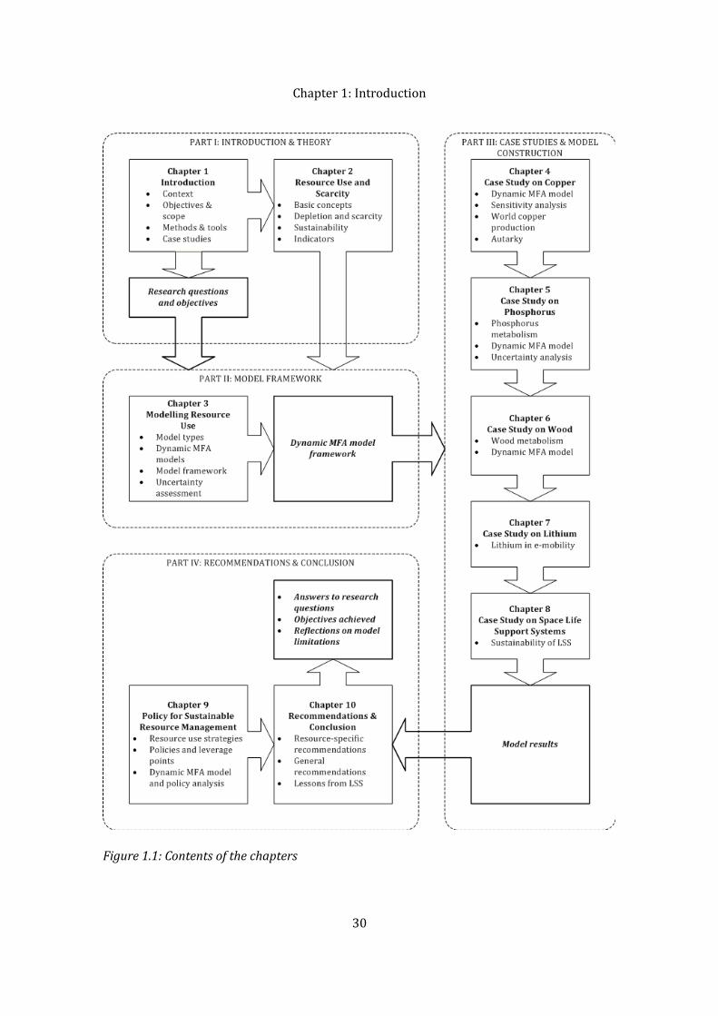
Chapter 1: IntroductionThe contents of the thesis are presented in schematic form in Figure 1.1. To ensure a fluid text unburdened by mathematical formulae, detailed model formulations and mathematical equations are for the most part presented in the Appendices. An Appendix is assigned to each case study apart from that on lithium: the copper case study is further detailed in Appendix B, phosphorus in Appendix C, wood in Appendix D, and space life support systems in Appendix E. The theoretical aspects related to Hubbert’s peak models of non-renewable resources are presented in Appendix A. In a policy-making context, the recommendations drawn from the Geneva case studies are summarized in Appendix F.

29

Chapter 1: Introduction

30Figure 1.1: Contents of the chapters

Chapter 1: Introduction1.7 TerminologyThe distinction between the terms ‘resource consumption’ and ‘resource use’ is not entirely clear. According to the Oxford English Dictionary (2011), consumption is the ‘action or fact of destroying or being destroyed’ or of ‘using something up in an activity’. Another definition is ‘the amount of goods, services, materials, or energy purchased and used’. Use, on the other hand, relates to ‘the act of putting something to work, or employing or applying a thing for any (especially a beneficial or productive) purpose’ or ‘utilization or appropriation, especially in order to achieve an end’. The difference between the two terms thus lies in the fact that resource consumption implies the destruction and degradation of the used materials while resource use refers to employing material resources to achieve a given societal purpose. On the other hand, the term ‘consumption’ can be merely used as a reference to a given quantity.In a recent UNEP report (UNEP 2011a), resource consumption is often used in contexts such as ‘per capita resource consumption’, ‘global resource consumption’, and ‘resource consumption rate’ referring to the amount of consumed goods while resource use is often used when speaking of environmental impacts, sustainability, and decoupling economic growth. However, the two terms are also often used synonymously. I have chosen to employ the term ‘resource use’ in the title of this thesis since it seems to be used in a wider variety of contexts than ‘resource consumption’ and is not limited to describing a given amount of materials or their use rate. Strictly speaking, the expression ‘sustainable resource consumption’ is an oxymoron as consumption implies the despoiling of the used material. In this thesis, the term ‘sustainability’ is employed often while the concept of ‘sustainable development’ is not addressed. Sustainable development is taken here to represent a political ideology whereas sustainability is seen as a property or characteristic of a system and the main focus of this study.

31

32

Chapter 2: Resource Use and ScarcityChapter 2 Resource Use and ScarcityResource use is a characteristic shared by all open, living systems. Apart from simplified systems models, there are in reality no isolated systems: all functioning systems interact with their environment in the form of materials and/or energy exchange. This chapter aims to analyse different aspects of resource use. It begins with a definition of basic resource use concepts (Chapter 2.1) and proceeds via concerns of resource depletion and scarcity (Chapter 2.2) to a discussion on the sustainability issues linked to resource use (Chapter 2.3). Lastly, resource use indicators such as autarky—expressing the degree of self-sufficiency—are examined in Chapter 2.4. 2.1 Basic Concepts and Definitions2.1.1 Typology of Natural ResourcesNatural resources are resources derived from the natural environment; according to one definition, they are ‘stocks of materials that exist in the natural environment that are both scarce and economically useful in production or consumption, either in their raw state or after a minimal amount of processing’ (WTO 2010). According to this definition, air is not considered a natural resource since human beings can obtain it freely by breathing. Neither is seawater a natural resource as it is neither scarce nor (in most cases) particularly useful from an economic standpoint. Manufactured goods require intensive processing and agricultural products are the result of cultivation rather than simple resource extraction. In this thesis, natural resources are often referred to simply as ‘resources’.Natural resources can be divided into the following categories (EC 2003):

– raw materials, such as minerals, fossil energy sources, and biomass– environmental media such as air, water, and soil– flow resources, notably wind, geothermal, tidal, and solar energy– physical space that provides the land surface used for human activities (settlements, infrastructure, industry, mineral extraction, agriculture, and forestry)

33

Chapter 2: Resource Use and ScarcityNatural resources are generally classified into renewable and non-renewable resources, the term ‘non-renewable’ referring to resources whose natural generation cycle is extremely long on a human time scale, such as fossil fuels, soil, or mineral deposits (EEA 2005). As a result, non-renewable resources can be regarded as finite, existing in a fixed, non-increasing stock on Earth, and all consumption thus diminishes their quantity irreversibly (EEA 2005). It has been pointed out that resources such as metals cannot actually be depleted in the same manner as fossil fuels, but they can be transformed from highly-concentrated and easily exploitable deposits to uneconomic diffuse sources as the entropy of the system increases.Non-renewable resources can also be called exhaustible, abiotic, or depletable resources. However, these terms are not completely interchangeable: for example, abiotic resources do not include soil, and the terms exhaustible and depletable can also be used in reference to renewable resources such as fisheries. Non-renewable resources might also be divided into recyclable resources (such as metals) and non-recyclable resources (such as fossil fuels).With regard to renewable resources, it is also possible to distinguish between flow and stock resources, or continuous and flow resources (resources available irrespective of human action versus resources capable of regenerating themselves but affected by human action). For more information of this subject, see Jowsey (2007). Renewable resources can also be classified into unconditionally and conditionally renewable resources (Jowsey 2007). 2.1.2 Mineral Resource Related ConceptsThis section briefly summarizes the central concepts related to mineral resources used in this thesis. These concepts are used in our case studies on copper, phosphorus, and lithium while the definitions related to renewable wood resources are presented in the next section (Chapter 2.1.3). According to the definitions of the United States Geological Survey (USGS 2009), the concepts ‘reserves’, ‘reserve base’ and ‘resources’ are differentiated as follows:

Reserve base.—That part of an identified resource that meets specified minimum physical and chemical criteria related to current mining and production practices, including those for grade, quality, thickness, and depth. The reserve base is the in-34

Chapter 2: Resource Use and Scarcityplace demonstrated (measured plus indicated) resource from which reserves are estimated. It may encompass those parts of the resources that have a reasonable potential for becoming economically available within planning horizons beyond those that assume proven technology and current economics. The reserve base includes those resources that are currently economic (reserves), marginally economic (marginal reserves), and some of those that are currently subeconomic (subeconomic resources).Reserves.—That part of the reserve base which could be economically extracted or produced at the time of determination. The term reserves need not signify that extraction facilities are in place and operative.Resource.—A concentration of naturally occurring solid, liquid, or gaseous material in or on the Earth’s crust in such form and amount that economic extraction of a commodity from the concentration is currently or potentially feasible.The term ‘resource base’, on the other hand, refers to the total amount of a material existing in or on the Earth’s crust (Tilton & Lagos 2007). The various resource and reserve definitions are summarized in Figure 2.1. It should be noted that reserves are a dynamic concept, changing in time in accordance with the technological developments, new discoveries, and economic realities. With regard to metal production, refined metal production attributable to mine production is named primary production, as it is obtained from primary raw materials (ICSG 2009). Another important source of metal raw materials is scrap: refined metal production derived from recycled scrap feed is referred to as secondary production (ICSG 2009).

35

Chapter 2: Resource Use and Scarcity

With regard to metal recycling, I have adopted the following vocabulary from the International Copper Study Group (ICSG 2009):The Recycling Input Rate (RIR) measures the proportion of metal and metal products that are produced from scrap and other metal-bearing low-grade residues. The RIR is mainly a statistical measurement for raw material availability and supply rather than an indicator of recycling efficiency of processes or products. ... Major 36

The image is not drawn to scale as the size of the resource base is usually substantial compared to the size of reserves and resources. ‘Other occurrences’ include non-conventional and low-grade materials.Source: adapted from Tilton & Lagos (2007) and USGS (2009).Figure 2.1: Reserve and resource definitions

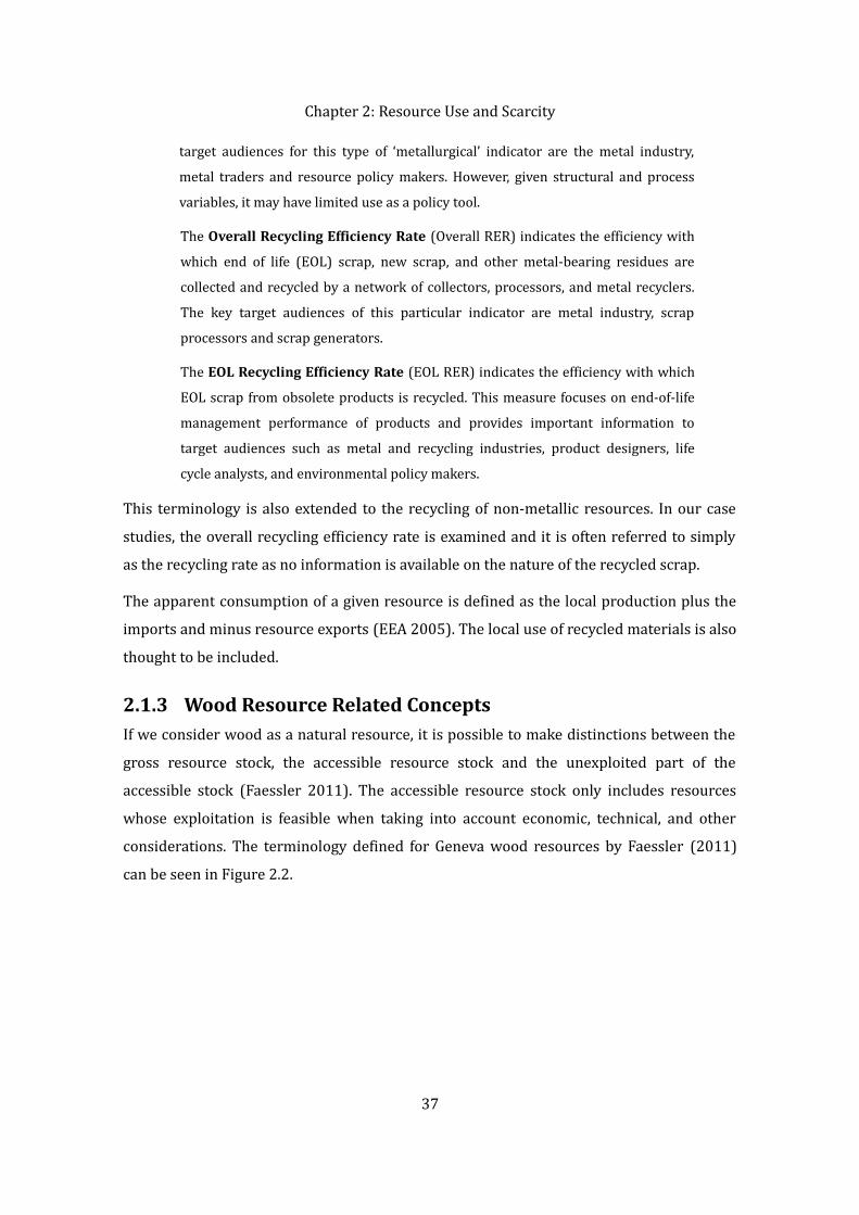
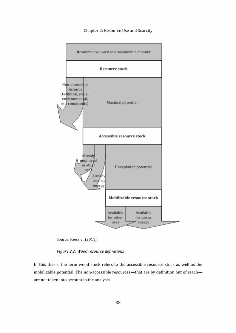
Chapter 2: Resource Use and Scarcitytarget audiences for this type of ‘metallurgical’ indicator are the metal industry, metal traders and resource policy makers. However, given structural and process variables, it may have limited use as a policy tool.The Overall Recycling Efficiency Rate (Overall RER) indicates the efficiency with which end of life (EOL) scrap, new scrap, and other metal-bearing residues are collected and recycled by a network of collectors, processors, and metal recyclers. The key target audiences of this particular indicator are metal industry, scrap processors and scrap generators.The EOL Recycling Efficiency Rate (EOL RER) indicates the efficiency with which EOL scrap from obsolete products is recycled. This measure focuses on end-of-life management performance of products and provides important information to target audiences such as metal and recycling industries, product designers, life cycle analysts, and environmental policy makers.This terminology is also extended to the recycling of non-metallic resources. In our case studies, the overall recycling efficiency rate is examined and it is often referred to simply as the recycling rate as no information is available on the nature of the recycled scrap. The apparent consumption of a given resource is defined as the local production plus the imports and minus resource exports (EEA 2005). The local use of recycled materials is also thought to be included. 2.1.3 Wood Resource Related ConceptsIf we consider wood as a natural resource, it is possible to make distinctions between the gross resource stock, the accessible resource stock and the unexploited part of the accessible stock (Faessler 2011). The accessible resource stock only includes resources whose exploitation is feasible when taking into account economic, technical, and other considerations. The terminology defined for Geneva wood resources by Faessler (2011) can be seen in Figure 2.2.

37

Chapter 2: Resource Use and Scarcity

In this thesis, the term wood stock refers to the accessible resource stock as well as the mobilizable potential. The non-accessible resources—that are by definition out of reach—are not taken into account in the analysis. 38

Source: Faessler (2011).Figure 2.2: Wood resource definitions

Chapter 2: Resource Use and Scarcity2.2 Resource Depletion and Scarcity 2.2.1 Defining ScarcityConcerns related to resource use and scarcity are not new: they can be traced back at least to Malthus and other classical economists of the 18th and 19th centuries. These concerns have since resurfaced regularly, for instance in the form of the famous Limits to Growth report commissioned by the Club of Rome (Meadows et al. 1972). Currently, the issue of resource shortage is of increasing concern in Switzerland (The Swiss Federal Council 2009) as well as all over the world. Besides concerns about resource availability in the current global context, scarcity also involves issues of justice and intergenerational equity: the Brundtland Commission report recommended that our resource management strategies should ensure that future generations neither suffer from the negative environmental impacts of our resource consumption nor be unable to satisfy their needs using the remaining natural resources (WCED 1987).Scarcity represents ‘an insufficiency of amount or supply’ (Wäger & Classen 2006). When speaking of mineral resources, the term ‘scarcity’ refers to the difference between the supply and demand of a given mineral (Wäger & Classen 2006). Scarcity can be caused by an increase in the demand for a resource that exceeds the increase in its availability or by a decrease in the availability of a resource that is greater than the decrease in its demand (Wäger & Classen 2006). Wäger and Classen (2006) distinguish two types of scarcity as follows:

– availability-related scarcity linked to• available mineral deposits• extraction rates• available anthropogenic stocks• recycling rates

– demand-related scarcity linked to• population growth and technological developmentThe concept of scarcity in relation to available mineral deposits and energy resources is a highly debated one and shall be examined in more detail in Chapter 2.2.2.

39

Chapter 2: Resource Use and ScarcityBeyond concerns regarding resource availability, an increasing amount of attention is paid to the negative environmental impacts of resource extraction, such as pollution, biodiversity loss, and climate change. This phenomenon has been called the ‘new scarcity’ and it is attracting an increasing amount of attention (see Simpson et al. 2004; Mudd & Ward 2008). In addition to economic and technological feasibility, decisions on resource extraction should also take into account environmental aspects, with the old concerns of physical shortage joining the more recent concerns of sustainable development.Resource quantities aside, there is also a problem of resource quality. The grade of a mineral ore usually declines along the exploitation process, as the highest-quality ore is exploited first, leaving only lower-quality deposits for later use. Therefore, in the absence of technological breakthroughs, the extraction costs as well as the required energy increase in order to continue processing poorer quality materials (Hussen 2004, pp. 369–370). Thus energy scarcity and the scarcity of various elements (especially metals) reinforce each other, as Diederen (2010) argues poignantly. However, it has recently been claimed that (at least in some cases) the decreasing ore grades are not driven by the depletion of high-grade deposits but result from the adoption of new extraction technologies that allow the treatment of previously sub-economic low-grade deposits (West 2011). In addition to basic resource quality issues, another potential problem for some elements is the existence of a mineralogical barrier: there may be a sharp discontinuity in the geochemical distribution of a mineral (Hussen 2004, p. 370). After the high-grade materials have been extracted, only diffuse, very low-grade sources remain (there is no smooth transition between the two source types in terms of cost or technology). This aspect remains relatively unknown and requires more research (National Research Council 1997).It is worthwhile noting that anthropogenic stocks have become important sources of resources, especially in the case of metals that can be recycled relatively easily (Gordon et al. 2006; Cohen 2007). These stocks have even been called above-the-ground, anthropogenic, or urban mines (Kapur & Graedel 2006; Graedel 2010). The availability of secondary resources is however limited by the following factors (Wäger & Classen 2006):– the quality of the materials that need to be recycled

40

Chapter 2: Resource Use and Scarcity– available recycling technologies in terms of available solutions, their costs and environmental impacts– the efficiency of these recycling technologies– interdependency and competitive aspects of the recycling technologies– the availability of auxiliary resources such as energy

2.2.2 Opposing Paradigms of Resource UseThere are two diametrically opposing views regarding non-renewable resources and the threat of their exhaustion. According to one viewpoint, the stocks of non-renewable resources are finite on a human time scale. When faced with growing resource demand—as a result of population growth and increasing living standards—the resource deposits decline and shall eventually run out. The second standpoint is that the actual size of the resource stocks is, on the contrary, irrelevant; it is more important to concentrate on the opportunity costs of finding and processing resources. As a resource becomes rarer, the opportunity costs as well as the resource price rise, causing consumers to seek more affordable substitutes. If the price rises sufficiently, the demand shall be depleted altogether although a substantial amount of resources may remain in the ground. Tilton (1996; 2003a; 2003b) has named these opposing viewpoints the opportunity cost and the fixed stock paradigm. The proponents of these views have also, in a somewhat enlarged context, been called growth optimists and pessimists (Mikesell 1995). The debate between the two opposing views is ongoing (see, for example, Maugeri 2004; Ehrenfeld 2005) and only the following can be deduced: It is clear that neither the optimists nor the pessimists currently have the needed evidence to prove the other side wrong. So perhaps the only reliable prediction one can make is that the debate will continue. Claims that mineral depletion unquestionably does, or does not, pose a serious threat to the welfare of modern civilization should be treated with some scepticism. (Tilton 2003a)This thesis is based on the fixed stock philosophy of which the Hubbert-type peak models are a renowned practical application (Hubbert’s peak models are presented in Chapter 2.2.3). This particular approach was chosen in order to concentrate on the evolution of physical stocks and flows of resources and not on economic aspects such as resource prices because the development of resource prices is notoriously difficult to predict. 41

Chapter 2: Resource Use and ScarcityHowever, I would argue that physical resource stocks are ultimately limited and therefore cannot last indefinitely when faced with exponential growing use of the Earth’s resources. It is not possible to rely indefinitely on the development of backstop resources that we can turn to when the original resource is depleted; we will ultimately have to face the physical limits of the planet. 2.2.3 Hubbert’s Peak Models

2.2.3.1 Characteristics of Hubbert’s Peak ModelThe original Hubbert’s peak model (Hubbert 1956) was created to model the production of fossil fuels (crude oil, coal, and gas) on a regional (Texas), national (the United States), and global scale. Hubbert (1956) drew the production curve in the shape of a symmetrical bell curve although his original paper made no reference to the curve’s mathematical formula, stating only:For any production curve of a finite resource of fixed amount, two points on the curve are known at the outset, namely that at t = 0 and then again at t = ∞. The production rate will be zero when the reference time is zero, and the rate will again be zero when the resource is exhausted; that is to say, in the production of any resource of fixed magnitude, the production rate must begin at zero, and then after passing through one

or several maxima, it must decline again to zero. … The only a priori information concerning the magnitude of the cumulative production of which we may be certain is that it will be less than, or at most equal to, the quantity of the resource initially present. Consequently, if we knew the quantity initially present, we could draw a family of possible production curves, all of which would exhibit the property of beginning and ending at zero, and encompassing an area equal to or less than the initial quantity. [My emphasis.]Hubbert applied his model to US crude oil production and predicted that it would reach its peak in the 1960s–70s. This did occur and Hubbert’s model became world-renowned. In his subsequent papers, Hubbert (1982) used a logistic growth function to describe the cumulative production curve. (For more information on the mathematical formulation of the model see Appendix A.) However, many other types of curves might be just as appropriate as is seen in the next section.

42

Chapter 2: Resource Use and ScarcityHubbert-type models have been applied to many different geological resources, ranging from fossil fuels (oil, gas, and coal) to metals and minerals, and even to biological resources such as fisheries (Bardi & Yaxley 2005). Interestingly, it was also suggested by Hubbert (1959) that cumulative discoveries follow a logistic curve in the same manner as the cumulative production. The cumulative production can therefore be predicted to reach the same asymptotic value as cumulative discoveries, but with a given time lag. Hubbert (1959) calculated a time lag of 10–11 years for the US crude oil production.2.2.3.2 Critique of Hubbert’s Peak ModelHubbert-type peak models have been criticized for a wide variety of reasons from technical to more philosophical aspects. Growth optimists challenge the model’s basic assumption of a limited resource stock while technical objections range from the shape of the curve to the limits of its applicability. The major problems posed by the model are presented briefly below. In Hubbert-type peak models, the production curve is presented as a derivative of the logistic function; however, this choice was made more or less arbitrarily and the production curve can also be surmised to take other forms. Brandt (2007) studied different types of oil production curves (linear, exponential, and bell-shaped growth) as well as the issues of symmetry. According to his conclusions, a bell-shaped curve is not always the best-fitting option. Brandt’s (2007) study shows that an asymmetric model (two exponential curves with different growth and decay rates) might be more fitting for oil production as the increase rate is usually higher than the decrease rate. The results also suggest that the production peak is often sharper than predicted by a bell-shaped curve: 40–50 of the 139 regions studied displayed this behaviour (Brandt 2007). (Brandt’s (2007) data were based on regional, national as well as multinational areas.) It is also worth noting that it is not clear whether Hubbert-type models are best applicable to the description of global, national, or smaller scale production. It is sometimes claimed that based on the Central Limit Theorem2 Hubbert’s peak models are particularly appropriate for large populations of fields or deposits (Laherrère 2000). But, according to 2 The Central Limit Theorem stipulates that when a sufficiently large number of independent variables (with their own mean and variance) are summed, the result shall approximate a normal distribution. 43

Chapter 2: Resource Use and ScarcityBrandt (2007), large production areas do not seem to appear to adhere to the model any more than smaller ones. It is also possible to imagine a multiple-cycle curve instead of a single-cycle curve; meaning that there would be more than one peak in the production of a resource. Examples of multi-peak oil production countries include, for instance, France and the UK (Laherrère 2000; Laherrère 2001). The multiple-peak model can be caused, for example, by the exploitation of different types of resources (e.g. offshore and onshore).It has been shown in the case of oil production that a large number of regions cannot be characterized by a Hubbert-type curve. In Brandt’s (2007) study, 16 regions out of 139 were disqualified as nonconforming and six more were labelled as borderline nonconforming (in total, 16% of the chosen regions). However, the Hubbert curve continues to provide a convenient and an easy-to-use estimate that is often employed for the lack of a better modelling method. 2.3 Resource Use and SustainabilityAs ‘new scarcity’ concerns demonstrate, resource use has wide implications for sustainability through the various production, consumption and waste creation processes related to it. There are essentially two ways in which the use of natural resources can endanger sustainable development (EC 2003): 1. Natural resource use can cause scarcity by depleting resources and thus threatening future development (economic as well as social).2. Natural resource use can generate environmental impacts that degrade environmental quality and thus put both ecosystems and human quality of life at risk.The sustainable use of natural resources therefore involves, firstly, ensuring their supply and, secondly, limiting the negative environmental impacts of their use (EC 2003).The sustainability of resource use can be approached for example in terms of ‘weak’ and ‘strong’ sustainability.

44

Chapter 2: Resource Use and Scarcity2.3.1 Weak and Strong SustainabilityThe concepts of weak and strong sustainability—originally defined by Pearce and Atkinson (1992)—analyse the relationship between the natural environment and the anthroposphere.3The definition of weak sustainability states that the sum of natural and manufactured capital must remain constant, i.e. the two types of capital are substitutable. There are several major problems with this definition, for instance one major difficulty resides in determining the value of various ecological assets, given the incommensurability of natural and man-made capital (Gallopín 2003). Another dilemma is posed by the fact that ecological resources are essential to all human activities and cannot be (fully) replaced with man-made capital. There is recognition that some environmental amenities and constituents (such as the Biosphere and its services) are irreplaceable and that impacts of some environmental processes (such as global warming) can be disastrous as well as irreversible (Gallopín 2003). It might therefore be preferable to ensure the sustainability of the global socio-ecological system and to employ the notion of strong sustainability. According to the strong sustainability concept, manufactured and natural capital are not always substitutable. Therefore, strong sustainability dictates that the stocks of natural capital should be maintained at the current level. Moreover, any evolution that implies a reduction in the natural capital stocks cannot be sustainable despite how much the stocks of man-made capital might increase (Gallopín 2003). 2.3.2 The Daly RulesThe ideas of strong sustainability are formulated more explicitly in the so-called Daly Rules (Daly 1990). The Daly Rules provide guidelines for the exploitation of renewable and non-renewable resources as well as for limiting waste creation (Daly 1990):

– Input rule for renewable resources: renewable resources should not be harvested faster than they can regenerate.– Input rule for non-renewable resources: the depletion rate of non-renewable resources should not exceed the rate at which renewable substitutes can be found.

3 Weak and strong sustainability have been further categorized into very weak, weak, strong, and very strong sustainability; however, these categories have not been further elaborated on here.45

Chapter 2: Resource Use and Scarcity– Output rule for wastes: waste emission rates should not exceed the assimilation capacities of the environment.Compared to the demands of strong sustainability, the Daly Rules include a concession permitting some use of non-renewable resources (should we follow the strong sustainability definition strictly, all natural capital should be kept intact). Some use of non-renewable resources is thus permitted, but how should this be regulated in practice? It is difficult to determine the rate at which renewable substitutes can be developed; indeed, for some resources, the main substitute remains another non-renewable resource.

2.3.3 Industrial Ecology ApproachIndustrial ecology concentrates on the biophysical substrata forming the basis of all human activities in the form of stocks and flows of materials and energy. These stocks and flows constitute the industrial metabolism which describes the resource use and waste creation processes of a system. Metabolism studies are an important aspect of the industrial ecology field. 2.3.3.1 Ecological RestructuringIn industrial ecology, the maturation strategy of industrial systems, or ecological restructuring, is presented as a way to achieve sustainability (Erkman 2004). The term ‘industrial system’ is used here in the industrial ecology sense, referring to all activities of the anthroposphere from raw materials extraction to agriculture, industry, commerce, and waste disposal. The four main objectives of the maturation strategy have been defined as follows (Erkman & Ramaswamy 2003, p. 6): 1. optimizing the use of resources2. closing material loops and minimizing emissions3. dematerializing activities4. reducing and eliminating the dependence on non-renewable sources of energyOptimizing the use of energy and materials aims to remove unnecessary losses. This rule is often said to be illustrated by the so-called eco-industrial parks where companies optimize their resource use by mutually recovering wastes and reusing and recycling them as raw materials.

46

Chapter 2: Resource Use and ScarcityThe second objective aims to remodel industrial activities as quasi-closed loop systems in the manner of natural ecosystems. The third objective states that the aim of industrial ecology is not only to create a cyclic system but also to minimize the flows of energy and matter involved in the process, the ultimate goal being to provide the same product or service with less materials and energy. Dematerialization can be further divided into relative—using a given amount of materials more efficiently so that it provides more goods and services—and absolute dematerialization aiming to reduce the absolute quantity of materials circulating within the economy. The fourth and final objective is to promote energy efficiency and the use of greener sources of energy.There has been much discussion about the most suitable approach to dematerialization (EEA 2005). Should we strive for the relative decoupling of economic growth from the environmental impacts of resource use? Or should we attempt a general dematerialization, promoting an absolute reduction in the use of resources? The advocates of the latter approach argue that it would be compatible with the precautionary principle and intergenerational equity (EEA 2005).2.3.3.2 The Ideal Industrial EcosystemAnother industrial ecology approach to formulating the demands of sustainability in terms of resource use is the concept of an ideal industrial ecosystem, a so-called type III ecosystem (Erkman 2004, p. 44). The ideal industrial ecosystem has been defined as a system that receives only (solar) energy from its environment while releasing heat; the system functions in a completely circular manner with respect to material resources (Richards et al. 1994, pp. 6–8). This is of course an idealization, in reality there would always be limited amounts of resource inputs and waste outputs. A schematic representation of the ideal industrial ecosystem can be seen in Figure 2.3.As industrial ecology is a science concerned with the physical flows of matter and energy underlying human activities, the ideal industrial ecosystem is consequently characterized by the nature of its interactions (materials and energy exchange) with the environment.

47

Chapter 2: Resource Use and Scarcity

2.4 Indicators of Sustainable Resource Use In the field of Life Cycle Analysis (LCA), indicators used to measure the consequences of resource use have been divided into four categories (Stewart & Weidema 2005; Steen 2006):– indicators based on aggregated energy or mass– indicators based on a measure of resource deposits and resource consumption – indicators based on potential economic and environmental impacts of resource extraction– indicators based on exergy consumption or entropy creationI shall present here briefly some possible indicators based on the relation of resource deposits and their consumption (Chapter 2.4.1). One particular indicator, autarky, whose use is illustrated in the copper case study, is presented in more detail in Chapter 2.4.2.The resource depletion indicators presented are especially adapted to non-renewable resources with a fixed stock while the sustainability of the use of renewable resources could be measured in a simpler manner with indicators such as the harvest rate/regeneration rate suggested by Meadows (1998). We could also define an indicator to measure the sustainability according to the third Daly rule (waste generation), for example emission rate/absorption rate (Meadows 1998). In a sustainable situation, the values of both these indicators should be less or equal to one. More direct measures could be

48

Source: Richards et al. (1994, pp.6-8). Figure 2.3: Ideal industrial ecosystem

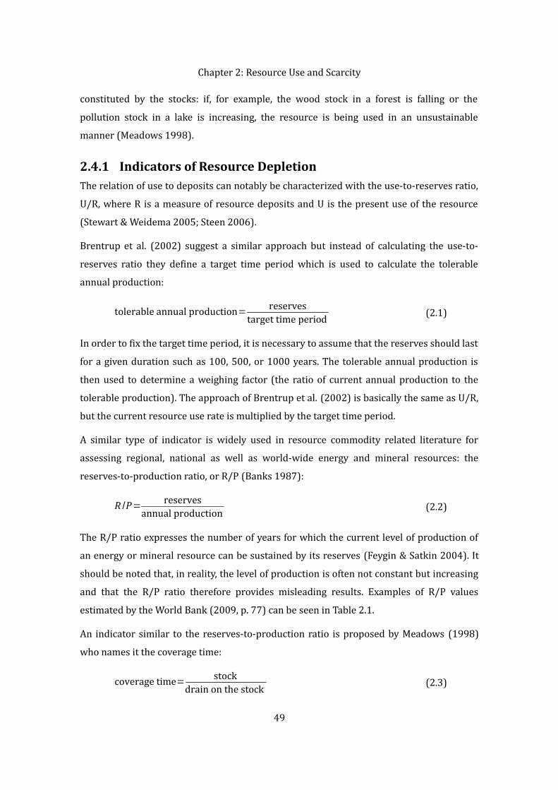
Chapter 2: Resource Use and Scarcityconstituted by the stocks: if, for example, the wood stock in a forest is falling or the pollution stock in a lake is increasing, the resource is being used in an unsustainable manner (Meadows 1998). 2.4.1 Indicators of Resource DepletionThe relation of use to deposits can notably be characterized with the use-to-reserves ratio, U/R, where R is a measure of resource deposits and U is the present use of the resource (Stewart & Weidema 2005; Steen 2006). Brentrup et al. (2002) suggest a similar approach but instead of calculating the use-to-reserves ratio they define a target time period which is used to calculate the tolerable annual production:

tolerable annual production= reservestarget time period (2.1)In order to fix the target time period, it is necessary to assume that the reserves should last for a given duration such as 100, 500, or 1000 years. The tolerable annual production is then used to determine a weighing factor (the ratio of current annual production to the tolerable production). The approach of Brentrup et al. (2002) is basically the same as U/R, but the current resource use rate is multiplied by the target time period.A similar type of indicator is widely used in resource commodity related literature for assessing regional, national as well as world-wide energy and mineral resources: the reserves-to-production ratio, or R/P (Banks 1987):

R /P= reservesannual production (2.2)The R/P ratio expresses the number of years for which the current level of production of an energy or mineral resource can be sustained by its reserves (Feygin & Satkin 2004). It should be noted that, in reality, the level of production is often not constant but increasing and that the R/P ratio therefore provides misleading results. Examples of R/P values estimated by the World Bank (2009, p. 77) can be seen in Table 2.1.An indicator similar to the reserves-to-production ratio is proposed by Meadows (1998) who names it the coverage time:

coverage time= stockdrain on the stock (2.3)49

Chapter 2: Resource Use and ScarcityThe use-to-reserves and the reserves-to-production indicators represent inverse values of one another when the production corresponds to the resource use.Table 2.1: Reserves-to-production ratios for various resources

Year Oil Coal Iron ore Copper Nickel Zinc1980 29 - 280 64 77 261990 42 - 178 41 53 212000 40 230 132 26 46 222007 42 133 79 31 40 17Source: World Bank (2008, p.77).The R/P ratio provides no information about the quality of the reserves, i.e. the ability to increase production (or to keep its level stable) for a prolonged period of time (Feygin & Satkin 2004). It has also been pointed out that although the R/P ratio might be quite considerable, for instance 40 years, this provides little comfort when world production attains its peak and begins to decline. It is therefore erroneous to think that even a sizeable R/P ratio would put any risk of supply difficulties well into the future (Bentley 2002). It has also been argued that the reserves-to-production ratio is unsuitable for prediction purposes; in fact, the R/P ratio of oil production in the United States has been about 10 years for the last 80 years (Laherrère 2005; Laherrère 2006)! This is due to the fact that reserves are in essence dynamic and not a fixed-size stock. It would therefore be more suitable to construct a predictive indicator based on, for instance, the resources or reserve base (as defined by the USGS) that are much less time-dependent. 2.4.2 Autarky

2.4.2.1 Definition of AutarkyThe degree of self-sufficiency or autarky was first defined by Oswald et al. (2003) in the context of urban planning as a means of describing the relationship between a region and its hinterlands. The indicator has been later used in the works of Redle (1999) and Nägeli (2008) who apply it to sustainable resource use on a regional scale. It can be expressed (in a somewhat simplified form) as: 50

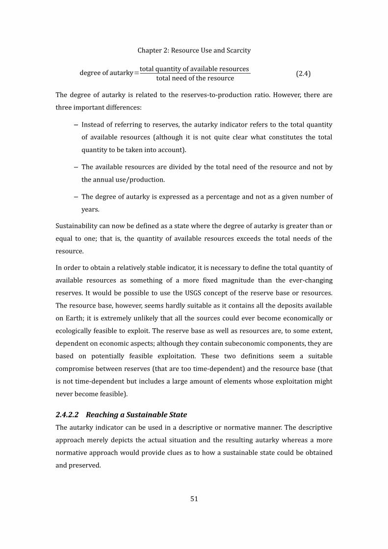
Chapter 2: Resource Use and Scarcitydegree of autarky=total quantity of available resourcestotal need of the resource (2.4)

The degree of autarky is related to the reserves-to-production ratio. However, there are three important differences:– Instead of referring to reserves, the autarky indicator refers to the total quantity of available resources (although it is not quite clear what constitutes the total quantity to be taken into account).– The available resources are divided by the total need of the resource and not by the annual use/production.– The degree of autarky is expressed as a percentage and not as a given number of years.Sustainability can now be defined as a state where the degree of autarky is greater than or equal to one; that is, the quantity of available resources exceeds the total needs of the resource.In order to obtain a relatively stable indicator, it is necessary to define the total quantity of available resources as something of a more fixed magnitude than the ever-changing reserves. It would be possible to use the USGS concept of the reserve base or resources. The resource base, however, seems hardly suitable as it contains all the deposits available on Earth; it is extremely unlikely that all the sources could ever become economically or ecologically feasible to exploit. The reserve base as well as resources are, to some extent, dependent on economic aspects; although they contain subeconomic components, they are based on potentially feasible exploitation. These two definitions seem a suitable compromise between reserves (that are too time-dependent) and the resource base (that is not time-dependent but includes a large amount of elements whose exploitation might never become feasible).

2.4.2.2 Reaching a Sustainable StateThe autarky indicator can be used in a descriptive or normative manner. The descriptive approach merely depicts the actual situation and the resulting autarky whereas a more normative approach would provide clues as to how a sustainable state could be obtained and preserved. 51

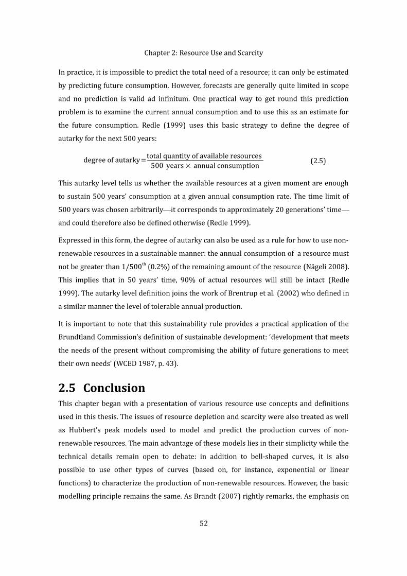
Chapter 2: Resource Use and ScarcityIn practice, it is impossible to predict the total need of a resource; it can only be estimated by predicting future consumption. However, forecasts are generally quite limited in scope and no prediction is valid ad infinitum. One practical way to get round this prediction problem is to examine the current annual consumption and to use this as an estimate for the future consumption. Redle (1999) uses this basic strategy to define the degree of autarky for the next 500 years:degree of autarky=total quantity of available resources500 years × annual consumption (2.5)

This autarky level tells us whether the available resources at a given moment are enough to sustain 500 years’ consumption at a given annual consumption rate. The time limit of 500 years was chosen arbitrarily—it corresponds to approximately 20 generations’ time—and could therefore also be defined otherwise (Redle 1999). Expressed in this form, the degree of autarky can also be used as a rule for how to use non-renewable resources in a sustainable manner: the annual consumption of a resource must not be greater than 1/500th (0.2%) of the remaining amount of the resource (Nägeli 2008). This implies that in 50 years’ time, 90% of actual resources will still be intact (Redle 1999). The autarky level definition joins the work of Brentrup et al. (2002) who defined in a similar manner the level of tolerable annual production. It is important to note that this sustainability rule provides a practical application of the Brundtland Commission’s definition of sustainable development: ‘development that meets the needs of the present without compromising the ability of future generations to meet their own needs’ (WCED 1987, p. 43). 2.5 ConclusionThis chapter began with a presentation of various resource use concepts and definitions used in this thesis. The issues of resource depletion and scarcity were also treated as well as Hubbert’s peak models used to model and predict the production curves of non-renewable resources. The main advantage of these models lies in their simplicity while the technical details remain open to debate: in addition to bell-shaped curves, it is also possible to use other types of curves (based on, for instance, exponential or linear functions) to characterize the production of non-renewable resources. However, the basic modelling principle remains the same. As Brandt (2007) rightly remarks, the emphasis on

52

Chapter 2: Resource Use and Scarcitynarrow technical issues often draws attention from more fundamental and important questions such as the nature of scarcity and the future of the energy system following the exhaustion of oil. Resource use and sustainability issues were also treated in this chapter: for instance, the notions of weak and strong sustainability, the Daly rules, and various principles of industrial ecology were presented. Indicators of sustainable resource use were also discussed and the autarky indicator was presented in more detail. This indicator could be used in a descriptive or normative manner either to describe the current degree of sustainability or to determine a maximum annual consumption level. However, the autarky indicator presents several disadvantages, notably the necessity to determine the total quantity of available resources, which cannot be established accurately on a 100% basis.

53

Thesis Structure

PART IIMODEL FRAMEWORK

56

Chapter 3: Modelling Resource UseChapter 3 Modelling Resource UseThis section presents the modelling aspects of the case studies on the Canton of Geneva. It begins with a short theoretical introduction to models in Chapter 3.1, including different model types, modelling in the field of industrial ecology as well as a few other common modelling methodologies in the sustainability domain. Following this, the choice of model is briefly justified (Chapter 3.1.4) and the chosen model type—dynamic MFA model—is presented in more detail in Chapter 3.2. Next, the construction of the dynamic MFA model framework—including the objectives of the modelling exercise, the model building principles, the basic hypotheses as well as the adaptation of the model to our various case studies—is described in Chapter 3.3. Uncertainty assessment in modelling is presented in Chapter 3.4, and a discussion and a conclusion follow in Chapters 3.5 and 3.6. 3.1 Introduction to Models3.1.1 Model Types and CharacteristicsThis section aims to give a brief overview of different types of models used to deal with sustainability issues. A ‘sustainability model’ is used to represent and study sustainability (Todorov & Marinova 2011). Generally speaking, different model types include for instance (Todorov & Marinova 2011):

– pictorial visualisations (graphical representations, images, and charts such as the Venn diagram)– quantitative models (such as mathematical, statistical, and econometric models as well as computer simulations)– physical models (scale models, physical representations, or other copies of the object of interest)– conceptual models (conceptualizations of a phenomenon of interest and theoretical ideas)– standardizing models (for instance indicators, indicator frameworks, and other performance measures)A short review of different types of sustainability models can be found in Todorov & Marinova (2011).

57

Chapter 3: Modelling Resource UseThe main characteristics of scientific models have been defined as follows (Franck 2002):1. Provide a simplified representation of the reality;2. Represent what is considered to be essential to this reality;3. Are testable;4. Under the scientific approach, the models themselves become the object of study;5. Are conceptual;6. Allow the possibility of measurement and calculation;7. Allow explanation of the reality;8. Are a fictive representation of the reality;9. Represent systems; and10. Are isomorphic … to the systems that they represent.All models should fulfil these characteristics. However, some types of models correspond to particular characteristics better than others (Todorov & Marinova 2011). The essence of models is captured by the first two criteria: models provide a simplified representation of the reality, representing only what is considered essential to the phenomenon under study. It is the purpose of the model that determines what is essential in its representation. Based on their purpose, models can be further classified as (Braat & Lierop 1987):1. descriptive models giving an overview of a given problem2. explanatory models aimed at clarifying system behaviour3. predictive models used to forecast future behaviour4. evaluative models used to assess alternativesThe model constructed in this thesis is a predictive model aimed at illustrating future behaviour. However, it is intended to provide more of a qualitative illustration than a precise quantitative prediction. As in the case of the Limits to Growth model, the purpose is ‘to give users a mental model of how changing the input for the various elements changes the output of the model’ and ‘to provide a fan of scenarios which would examine and evaluate various “what if” hypotheses’ (Bardi 2011, p. 43). A scenario is defined as one of several possible outcomes resulting from a simulation (Bardi 2011, p. 16). Performing a 58

Chapter 3: Modelling Resource Usesimulation, on the other hand, ‘means that the model’s equations are solved stepwise as a function of time; usually using a computer’ (Bardi 2011, p. 16).From a policy-making point of view, sustainability issues often pose particular challenges that must be taken into account in choosing the modelling approach; these challenges include notably human–nature interactions, uncertainties, as well as temporal, spatial and social externalities (Boulanger & Bréchet 2005). The proposed methodological answers to these problems are summarized in Table 3.1. Table 3.1: Sustainability problems and methodological answers

Problem Methodological AnswerHuman–nature interactions Interdisciplinary approachUncertainties Managing uncertaintyTemporal externalities Long-range or intergenerational point of viewSpatial externalities Global-local perspectiveSocial externalities Stakeholders’ participationSource: Boulanger & Bréchet (2005). Models used in the field of industrial ecology are often quantitative models although a more conceptual approach is sometimes used; the industrial ecology modelling domain is presented in more detail in the following section. Other commonly used modelling methodologies for sustainability issues are treated briefly in Chapter 3.1.3 and the chosen model type is unveiled in Chapter 3.1.4. 3.1.2 Modelling in Industrial EcologyThis section aims to present several quantitative modelling methodologies used in the field of sustainability in general and in industrial ecology applications in particular. These modelling methodologies include life cycle assessment, material and substance flow analysis, and industrial symbiosis.

59

Chapter 3: Modelling Resource Use3.1.2.1 Life Cycle AssessmentLife Cycle Assessment or Analysis (LCA) is a methodology measuring the potential environmental impacts created by a given product or a service during its entire life cycle in a cradle-to-grave approach. The ISO framework for LCA defines the following four phases for LCA studies: the definition of the goal and scope of the study, life cycle inventory analysis, life cycle impact assessment, and life cycle interpretation (ISO 2011). In the first definition phase, the object of study is described and delimited in terms of a so-called functional unit. The second inventory phase involves data collection and modelling of the system, which is usually done with the help of dedicated software packages. The third impact assessment phase is aimed at evaluating the contribution to various impact categories (representing environmental issues of concern) such as climate change, ozone depletion, ecotoxicity, or acidification. The impact categories can also be assigned different weights according to their importance. In the last interpretation phase of LCA, the results are related to the goal of the study as defined in the beginning. For an introduction to life cycle assessment, see, for example, Guinée (2002).3.1.2.2 Material Flow AnalysisMaterial Flow Analysis (MFA) is a systematic assessment of the stocks and flows of materials related to a well-defined system in space and time. MFA delivers a complete and consistent set of information about the flows passing through and the stocks of materials accumulating within a chosen system. In MFA terminology, ‘material’ stands for both substances and goods (Brunner & Rechberger 2004). A substance is defined as a single type of matter consisting of uniform units (e.g. zinc, iron, carbon dioxide, or water) whereas goods are substances or mixtures of substances with an economic value, either positive or negative (Brunner & Rechberger 2004). According to this definition, three of our case study materials (copper, phosphorus, and lithium) are substances while the fourth (wood) is a good. A material flow analysis concentrated solely on substances can also be called a Substance Flow Analysis (SFA). National- and regional-level material flow analysis is often referred to as Material Flow Accounting while material and energy flows related to the life cycle of a product or a service are a part of the life cycle inventory step of life cycle assessment. Traditional MFA approaches are static, providing only a fixed view on the stocks and flows of a system. However, the MFA approach has also been developed in a dynamic form and it 60

Chapter 3: Modelling Resource Usehas been used to simulate historic metabolism as well as to predict future evolutions (see, for example, Spatari et al. 2005; Hatayama et al. 2010). Another use of dynamic MFA is to exploit data on past stock and flow behaviour to foresee future emissions of pollutants and waste (see, for example, Voet et al. 2002; Elshkaki et al. 2005). The usefulness and limitations of MFA/SFA studies in environmental decision-making have been succinctly summarized by Antikainen (2007, p. 5): ‘SFA is not usually sufficiently detailed to allow specific recommendations for decision-making to be made, but it does yield useful information about the relative magnitude of the flows and may reveal unexpected losses. SFA studies should be supported with other methods such as LCA. Data uncertainties are high in this type of analysis. Use of quantitative uncertainty analysis is therefore recommended. Definition of the system boundaries significantly affects conclusions drawn from SFA results.’ 3.1.2.3 Industrial SymbiosisIndustrial symbiosis (or industrial biocenosis) can be defined as the sharing of information, by-products, and other resources among industrial players in order to add value, cut down costs, and lessen negative environmental impacts (Agarwal & Strachan 2008). Industrial symbiosis studies often focus on material and energy exchanges as in the case of the Kalundborg symbiosis, which is a much-used textbook example. For a presentation of the Kalunborg symbiosis, see, for example, Erkman and Ramaswamy (2003, pp. 10–14) or Erkman (2004, pp. 28–32). Aside from Kalundborg, industrial symbioses have been studied all over the globe; examples include, for instance, a recycling network in Styria, an Austrian province (Posch 2010); the Barceloneta region on the island of Puerto Rico (Ashton 2009); the Burnside Industrial Park in Canada (Wright et al. 2009) as well as various industrial estates in India (Bain et al. 2010), Eco-Town projects in Japan (Morioka et al. 2005), and the Guitang Group in China (Zhu et al. 2008).3.1.3 Other Modelling MethodologiesThree commonly used modelling methodologies in sustainability applications (input-output models, agent-based models, and system dynamics models) are briefly presented in this section. Besides these methodologies, there are also many others (such as econometric models, computable general equilibrium models, optimization models, and Bayesian networks) that are not presented here further. A brief presentation of different

61

Chapter 3: Modelling Resource Usemodel types along with examples of their application can be found in Boulanger and Bréchet (2005). Various models related to sustainable materials management have also been described by the OECD (2008a).3.1.3.1 Input-Output ModelsAn input-output model is a quantitative econometric tool representing in a matrix form the economy of a nation or a region. Input-output models can be used to predict how changes in one industry affect other economic sectors as well as consumers, the government and foreign suppliers and buyers in the economy. The mathematical formulation of input-output models is quite straightforward; however, the data requirements are often consequential as the transactions of each branch of economic activity must be characterized quantitatively.3.1.3.2 Agent-Based ModelsAn agent-based model or a multi-agent simulation is a computational model used for simulating the actions and interactions of various autonomous agents. The ‘agents’ represent both individual and collective entities such as groups or organizations. The aim of agent-based modelling is to shed light on the combined effects of the agents’ actions on the system. Agent-based modelling combines influences from different mathematical and systemic disciplines such as game theory, complex systems, and emergence. Simple rules on agent responses can create complex collective behaviour.3.1.3.3 System Dynamics ModelsSystem dynamics aims at modelling the behaviour of complex systems over time while taking into account their positive and negative feedback loops as well as various delay phenomena. Two illustrative tools are often used in the field: stock-flow models and causal loop diagrams. Due to their simplicity, causal loop diagrams are often used to visualize and conceptualize the positive and negative feedback loops within a system. However, the very simplicity of causal loop diagrams may lead to misunderstandings and misinterpretations (Richardson 1986). Stock-flow diagrams are more suited to modelling and have been used in various environmental applications, for example in water management (Winz et al. 2008). System dynamics modelling can also be done without creating visual stock-flow diagrams, by using purely mathematical models with difference or differential equations. The World3

62

Chapter 3: Modelling Resource Usemodel of The Limits to Growth (Meadows et al. 1972) was in essence a mathematical system dynamics model implemented in the DYNAMO language. The Limits to Growth model was based on the World2 model of J.W. Forrester (1971), the father of system dynamics. 3.1.4 Required Model Characteristics and Model ChoiceThe case studies in the Canton of Geneva presented deal with regional resource metabolism in a medium and long-term perspective. As the aim of the study was to provide practical guidelines for sustainable resource management, the chosen model needed to provide quantitative projections for the development of resource use in the Canton. The model requirements can therefore be summarized as:

– adapted to regional level– quantitative– dynamic– predictiveThe different modelling categories and their characteristics are summarized in Table 3.2. The four model requirements direct us towards the model family of dynamic MFA models. This model type also provides answers to the challenges of modelling human–nature relationships and takes into account temporal externalities: our approach could be characterized as interdisciplinary as well as providing a long-term perspective (Boulanger & Bréchet 2005). The field of industrial ecology is profoundly interdisciplinary by nature, combining environmental, social as well as technical aspects. The use of ‘equation-based’ techniques (notably dynamic material flow analysis) and agent-based modelling in industrial ecology applications were compared in a recent article (see Bollinger et al. 2011). Agent-based models are especially adapted to situations where the roles and rationality of specific actors are central to system behaviour. However, as this was not the case in our application, I have chosen to employ the more simple and traditional approach of dynamic MFA.

63

Chapter 3: Modelling Resource UseTable 3.2: Synthesis of modelling methodologies

Modelling Methodology

System of Interest

Static vs.Dynamic Model

Descriptive vs. Predictive ModelMaterial flow analysis Any well defined system (company, industry, region, state, etc.)

Static (/Dynamic) DescriptiveLife cycle assessment Product, service Static DescriptiveIndustrial symbiosis Industrial park, region Static DescriptiveInput-output models Region, state, etc. Static Predictive (in the short-term)Agent-based models Any system with several ‘agents’ Dynamic Descriptive/ PredictiveSystem dynamics models Any system Dynamic Descriptive/ Predictive

In conclusion, a dynamic material flow analysis model was constructed. This choice has been made for two main reasons:1. As we are dealing with regional metabolism (the aim is to study the evolution of material stocks and flows within the Canton of Geneva in a quantitative manner), it seems natural to use the material flow analysis tool. 2. Traditional MFA approaches provide only a static snapshot of a given situation; since our aim is to include a dynamic, predictive aspect, it is necessary to enhance the MFA methodology with aspects of dynamic modelling.The family of dynamic MFA models is presented in detail in the following section. With dynamic MFA models, future evolutions can be traced. These models are thus adapted to prospective and strategic decision-making.

64

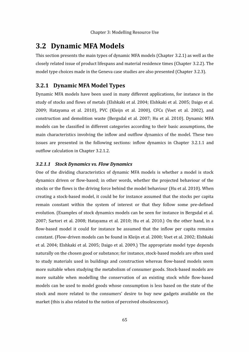
Chapter 3: Modelling Resource Use3.2 Dynamic MFA ModelsThis section presents the main types of dynamic MFA models (Chapter 3.2.1) as well as the closely related issue of product lifespans and material residence times (Chapter 3.2.2). The model type choices made in the Geneva case studies are also presented (Chapter 3.2.3). 3.2.1 Dynamic MFA Model TypesDynamic MFA models have been used in many different applications, for instance in the study of stocks and flows of metals (Elshkaki et al. 2004; Elshkaki et al. 2005; Daigo et al. 2009; Hatayama et al. 2010), PVC (Kleijn et al. 2000), CFCs (Voet et al. 2002), and construction and demolition waste (Bergsdal et al. 2007; Hu et al. 2010). Dynamic MFA models can be classified in different categories according to their basic assumptions, the main characteristics involving the inflow and outflow dynamics of the model. These two issues are presented in the following sections: inflow dynamics in Chapter 3.2.1.1 and outflow calculation in Chapter 3.2.1.2. 3.2.1.1 Stock Dynamics vs. Flow DynamicsOne of the dividing characteristics of dynamic MFA models is whether a model is stock dynamics driven or flow-based; in other words, whether the projected behaviour of the stocks or the flows is the driving force behind the model behaviour (Hu et al. 2010). When creating a stock-based model, it could be for instance assumed that the stocks per capita remain constant within the system of interest or that they follow some pre-defined evolution. (Examples of stock dynamics models can be seen for instance in Bergsdal et al. 2007; Sartori et al. 2008; Hatayama et al. 2010; Hu et al. 2010.) On the other hand, in a flow-based model it could for instance be assumed that the inflow per capita remains constant. (Flow-driven models can be found in Kleijn et al. 2000; Voet et al. 2002; Elshkaki et al. 2004; Elshkaki et al. 2005; Daigo et al. 2009.) The appropriate model type depends naturally on the chosen good or substance; for instance, stock-based models are often used to study materials used in buildings and construction whereas flow-based models seem more suitable when studying the metabolism of consumer goods. Stock-based models are more suitable when modelling the conservation of an existing stock while flow-based models can be used to model goods whose consumption is less based on the state of the stock and more related to the consumers’ desire to buy new gadgets available on the market (this is also related to the notion of perceived obsolescence).

65

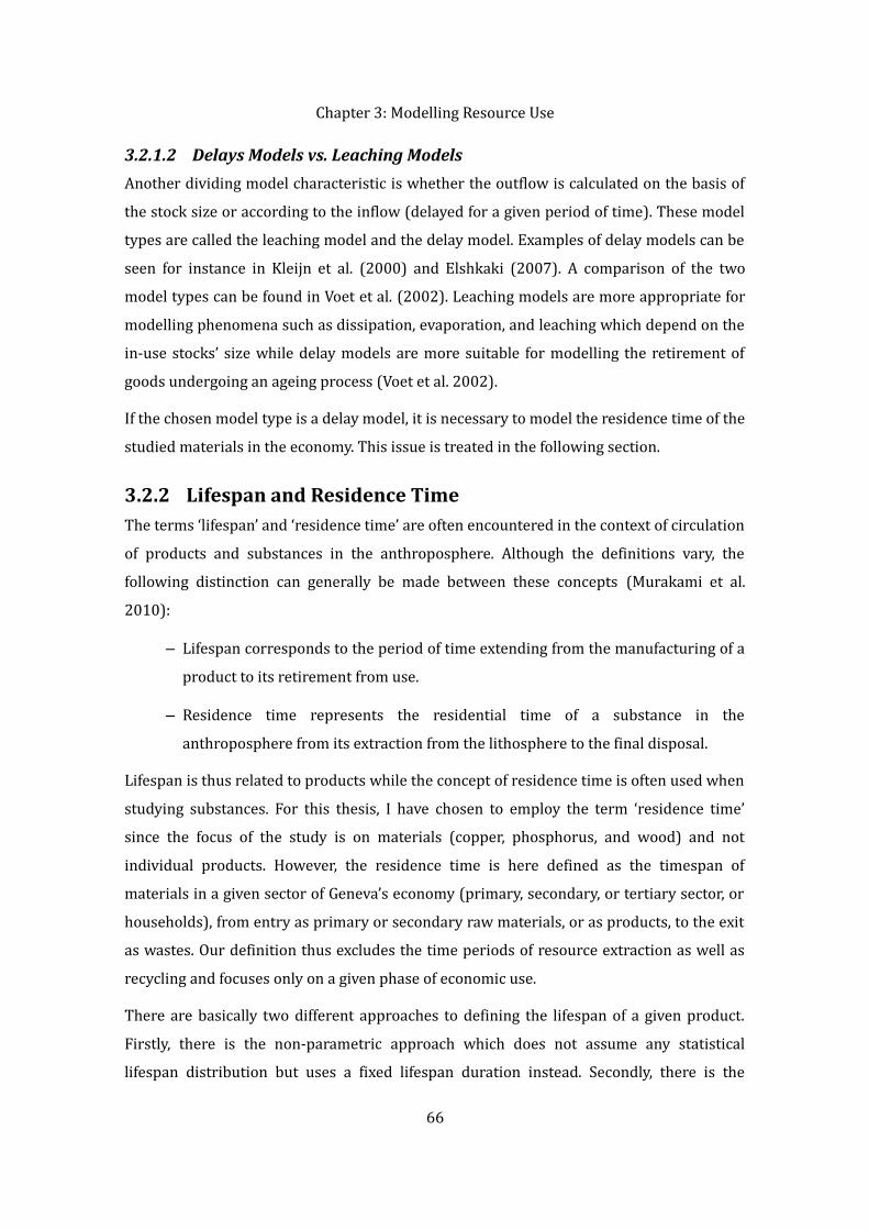
Chapter 3: Modelling Resource Use3.2.1.2 Delays Models vs. Leaching ModelsAnother dividing model characteristic is whether the outflow is calculated on the basis of the stock size or according to the inflow (delayed for a given period of time). These model types are called the leaching model and the delay model. Examples of delay models can be seen for instance in Kleijn et al. (2000) and Elshkaki (2007). A comparison of the two model types can be found in Voet et al. (2002). Leaching models are more appropriate for modelling phenomena such as dissipation, evaporation, and leaching which depend on the in-use stocks’ size while delay models are more suitable for modelling the retirement of goods undergoing an ageing process (Voet et al. 2002). If the chosen model type is a delay model, it is necessary to model the residence time of the studied materials in the economy. This issue is treated in the following section. 3.2.2 Lifespan and Residence TimeThe terms ‘lifespan’ and ‘residence time’ are often encountered in the context of circulation of products and substances in the anthroposphere. Although the definitions vary, the following distinction can generally be made between these concepts (Murakami et al. 2010):

– Lifespan corresponds to the period of time extending from the manufacturing of a product to its retirement from use. – Residence time represents the residential time of a substance in the anthroposphere from its extraction from the lithosphere to the final disposal. Lifespan is thus related to products while the concept of residence time is often used when studying substances. For this thesis, I have chosen to employ the term ‘residence time’ since the focus of the study is on materials (copper, phosphorus, and wood) and not individual products. However, the residence time is here defined as the timespan of materials in a given sector of Geneva’s economy (primary, secondary, or tertiary sector, or households), from entry as primary or secondary raw materials, or as products, to the exit as wastes. Our definition thus excludes the time periods of resource extraction as well as recycling and focuses only on a given phase of economic use.There are basically two different approaches to defining the lifespan of a given product. Firstly, there is the non-parametric approach which does not assume any statistical lifespan distribution but uses a fixed lifespan duration instead. Secondly, there is the

66

Chapter 3: Modelling Resource Useparametric approach which is based on a given distribution function, such as normal, log-normal, or Weibull distribution (Oguchi et al. 2010). Often, not much data is available on the lifespans of various products. However, lifespan distributions can be estimated in different ways (for more information see Oguchi et al. 2010). 3.2.3 Choice of the Model TypeFor this thesis, I have chosen to construct a model driven by flow dynamics. A flo w-driven model can be argued to suit the three substances studied, namely copper, phosphorus, and wood.Phosphorus fertilizers (which account for a significant usage of phosphorus in the Canton of Geneva) must be reapplied yearly to ensure the growth of plants. A flow-driven model seems therefore fairly realistic. However, it might also be argued that phosphorus nutrients constitute a stock in the soil and that this stock should be kept constant. This latter approach would, however, require a significant amount of knowledge on soil-chemistry. In addition, phosphorus is continuously removed from soil via run-off and erosion. Wood is largely used in Switzerland as wood energy and new input is therefore needed yearly: one study estimated that 69% of the wood consumed in Switzerland (including local production as well as net imports) served energy purposes (FOEN 2009b). Packaging is another major short-term usage of wood. However, an older study from the Canton of Geneva found that short time-scale uses (wood energy and packaging) represent merely 21% of the total use (Faist Emmenegger & Frischknecht 2003). A stock-driven model might therefore be argued to be suitable if a significant amount of wood is used in construction, buildings, and in other long-term applications. However, as the results of this early study are fairly uncertain, other more recent data underlining the importance of wood energy have been used.The choice of model in the case of copper is also a tricky one. Copper is widely employed in consumer electronics and various home appliances as well as in buildings and construction. However, it has been shown that the copper stocks per capita have continued to grow in the 20th century, at least in the US (Gordon et al. 2006). As stocks per capita cannot be assumed to remain constant, it seems more logical to assume that the copper

67

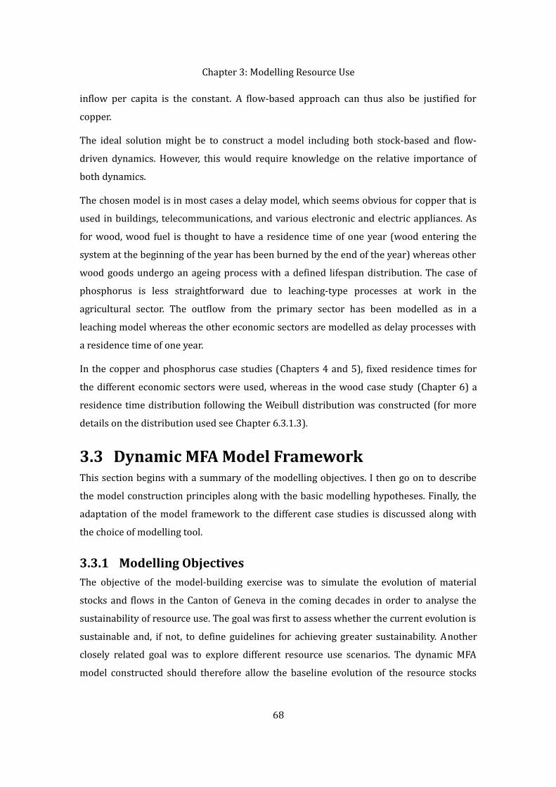
Chapter 3: Modelling Resource Useinflow per capita is the constant. A flow-based approach can thus also be justified for copper.The ideal solution might be to construct a model including both stock-based and flow-driven dynamics. However, this would require knowledge on the relative importance of both dynamics.The chosen model is in most cases a delay model, which seems obvious for copper that is used in buildings, telecommunications, and various electronic and electric appliances. As for wood, wood fuel is thought to have a residence time of one year (wood entering the system at the beginning of the year has been burned by the end of the year) whereas other wood goods undergo an ageing process with a defined lifespan distribution. The case of phosphorus is less straightforward due to leaching-type processes at work in the agricultural sector. The outflow from the primary sector has been modelled as in a leaching model whereas the other economic sectors are modelled as delay processes with a residence time of one year. In the copper and phosphorus case studies (Chapters 4 and 5), fixed residence times for the different economic sectors were used, whereas in the wood case study (Chapter 6) a residence time distribution following the Weibull distribution was constructed (for more details on the distribution used see Chapter 6.3.1.3).3.3 Dynamic MFA Model FrameworkThis section begins with a summary of the modelling objectives. I then go on to describe the model construction principles along with the basic modelling hypotheses. Finally, the adaptation of the model framework to the different case studies is discussed along with the choice of modelling tool. 3.3.1 Modelling ObjectivesThe objective of the model-building exercise was to simulate the evolution of material stocks and flows in the Canton of Geneva in the coming decades in order to analyse the sustainability of resource use. The goal was first to assess whether the current evolution is sustainable and, if not, to define guidelines for achieving greater sustainability. Another closely related goal was to explore different resource use scenarios. The dynamic MFA model constructed should therefore allow the baseline evolution of the resource stocks

68

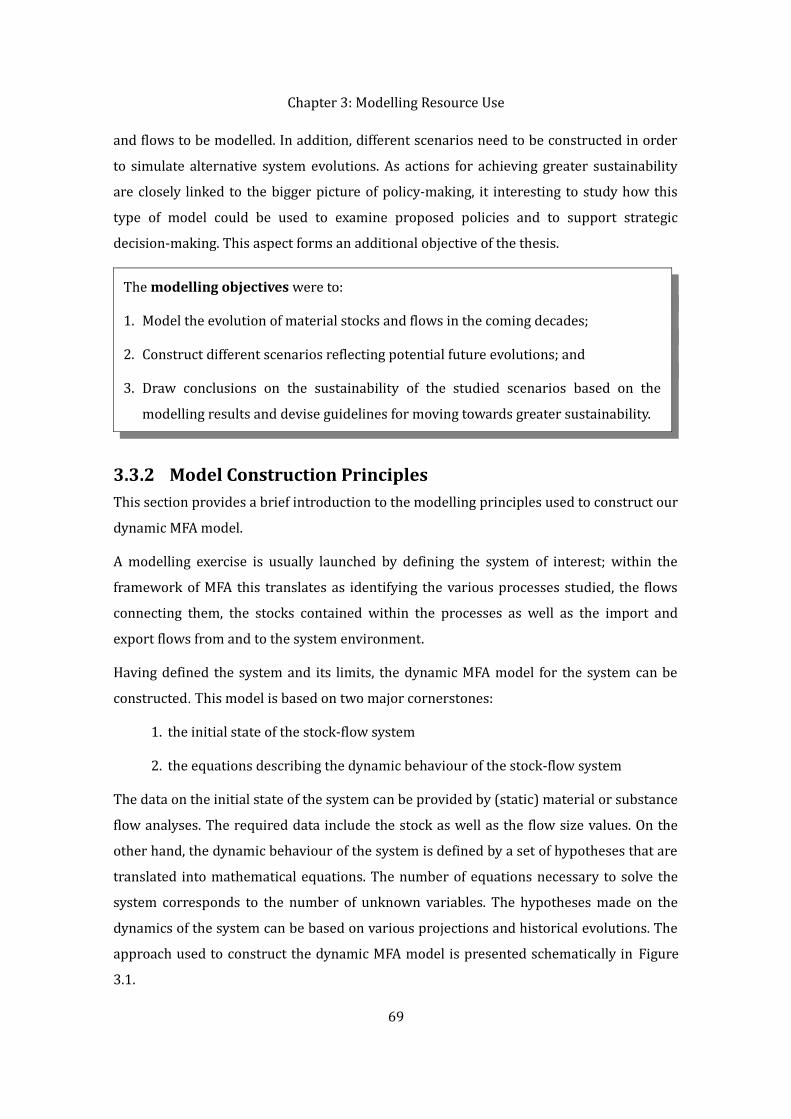
Chapter 3: Modelling Resource Useand flows to be modelled. In addition, different scenarios need to be constructed in order to simulate alternative system evolutions. As actions for achieving greater sustainability are closely linked to the bigger picture of policy-making, it interesting to study how this type of model could be used to examine proposed policies and to support strategic decision-making. This aspect forms an additional objective of the thesis.The modelling objectives were to:1. Model the evolution of material stocks and flows in the coming decades;2. Construct different scenarios reflecting potential future evolutions; and3. Draw conclusions on the sustainability of the studied scenarios based on the modelling results and devise guidelines for moving towards greater sustainability.

3.3.2 Model Construction PrinciplesThis section provides a brief introduction to the modelling principles used to construct our dynamic MFA model.A modelling exercise is usually launched by defining the system of interest; within the framework of MFA this translates as identifying the various processes studied, the flows connecting them, the stocks contained within the processes as well as the import and export flows from and to the system environment.Having defined the system and its limits, the dynamic MFA model for the system can be constructed. This model is based on two major cornerstones:1. the initial state of the stock-flow system2. the equations describing the dynamic behaviour of the stock-flow systemThe data on the initial state of the system can be provided by (static) material or substance flow analyses. The required data include the stock as well as the flow size values. On the other hand, the dynamic behaviour of the system is defined by a set of hypotheses that are translated into mathematical equations. The number of equations necessary to solve the system corresponds to the number of unknown variables. The hypotheses made on the dynamics of the system can be based on various projections and historical evolutions. The approach used to construct the dynamic MFA model is presented schematically in Figure3.1. 69

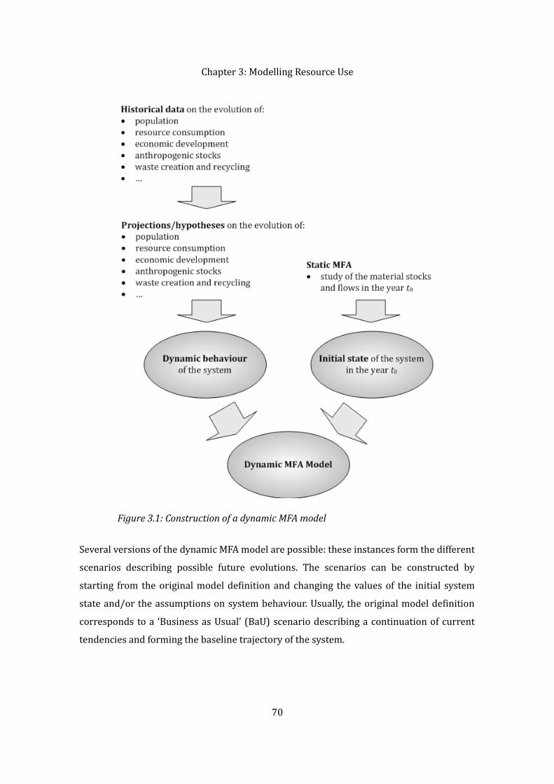
Chapter 3: Modelling Resource Use

Several versions of the dynamic MFA model are possible: these instances form the different scenarios describing possible future evolutions. The scenarios can be constructed by starting from the original model definition and changing the values of the initial system state and/or the assumptions on system behaviour. Usually, the original model definition corresponds to a ‘Business as Usual’ (BaU) scenario describing a continuation of current tendencies and forming the baseline trajectory of the system.

70

Figure 3.1: Construction of a dynamic MFA model

Chapter 3: Modelling Resource Use3.3.3 Basic Hypotheses

3.3.3.1 TerminologyBefore defining the model dynamics, the following precision is needed on the terminology employed: – Imports represent input flows from outside the system limits.– Exports represent output flows to the system environment; exports can generally be divided in to exports of products and exports of recycled materials.

– Net imports correspond to imports minus product exports (recycled material exports are excluded).– The amount of recycled materials represent all the waste that is collected to be recycled; this flow can be further divided into recycled materials that are consumed within the system and exports of materials to be recycled outside the Canton.– The total consumption corresponds to imports plus the consumption of recycled materials used within the system.– Apparent consumption corresponds to net imports plus the consumption of recycled materials within the system.– The required amount of primary materials is defined as net imports minus the amount of recycled materials (these recycled materials might or might not be exported).When referring to metals, it is also possible to speak about secondary materials; this term represents recycled materials. The conventions are summarized in Figure 3.2. The required amount of primary materials also takes into account the exports of recycled materials since they contribute to decreasing the consumption of primary materials in the Canton, at least in an indirect manner. For instance, the Canton has no copper recycling industry and all copper scrap must therefore be treated outside the Canton. To simplify matters, it was considered that this recycled copper later returns to the Canton as secondary refined copper or in copper products. In addition, the terms in-use stocks and anthropogenic stocks are employed. In-use stocks represent the stocks in various economic sectors (primary, secondary, and tertiary 71

Chapter 3: Modelling Resource Usesectors as well as the households) while anthropogenic stocks refer to all resource stocks during their usage and afterwards (i.e. stocks in the economic sectors as well as in landfills).

3.3.3.2 Model DynamicsIn this thesis, it is assumed that the apparent consumption remains proportional to the population: the resource needs increase in a linear manner in accordance with the population size. Therefore, in order to determine the quantity of resource needs, it is necessary to, firstly, model the population growth and, secondly, to determine the resource needs per capita. Population projections are examined in Chapter 3.3.3.3. The resource needs per capita are determined for each substance studied based on existing material flow analyses (for more information, see the sections that deal with the case studies). In order to simplify the analysis, the resource needs per capita are thought to remain constant. An assumption that the resource needs (i.e. apparent consumption) are proportional to the population means in practice that the current living standards are predicted to remain the same as population numbers rise. In this case, living standards are linked to the system inflows.72

Figure 3.2: System terminology

Chapter 3: Modelling Resource UseIn addition, it is assumed that the relative sizes of the import and export flows related to different economic sectors remain constant. This assumption is made since no information is available on future evolutions in the sectors. Two different assumptions can be made with regard to the waste flows: it can either be assumed that the waste flows leaving the system correspond to the system inflows with a given delay, i.e. a lifespan, or that the outflows are proportional to the stock size. The first assumption corresponds to a situation where the consumed goods are used over a certain period and then discarded as waste (a delay model) whereas the second situation describes phenomena related to leaching, erosion, and diffusion (a leaching model).It is assumed that the relative sizes of the system outflows (recycled and landfilled waste, etc.) remain the same.Model Hypothesis 1: Apparent consumption remains directly proportional to the population. Model Hypothesis 2: The relative sizes of the import and export flows related to the different economic sectors remain constant.Model Hypothesis 3a: The waste flows correspond to the system inflows delayed by a given lifespan. Model Hypothesis 3b: The waste flows are proportional to the stock size.Model Hypothesis 4: The relative sizes of the system outflows remain unchanged.

3.3.3.3 Population ProjectionsAs it is assumed that the materials consumption in the Canton of Geneva is linked to the number of inhabitants, the Geneva population constitutes the driving socio-economic variable of our model. Let us examine closer the future evolution of the Geneva population.The population projections used in this thesis (Table 3.3) are forecasts established by OCSTAT, the Cantonal Statistical Office of Geneva. The scenarios A–D indicate possible future evolutions whereas A1 and E are more speculative possibilities (OCSTAT 2005c). E is a purely theoretical zero influx scenario whereas A1 assumes an increase in the birth rate (OCSTAT 2005c). 73

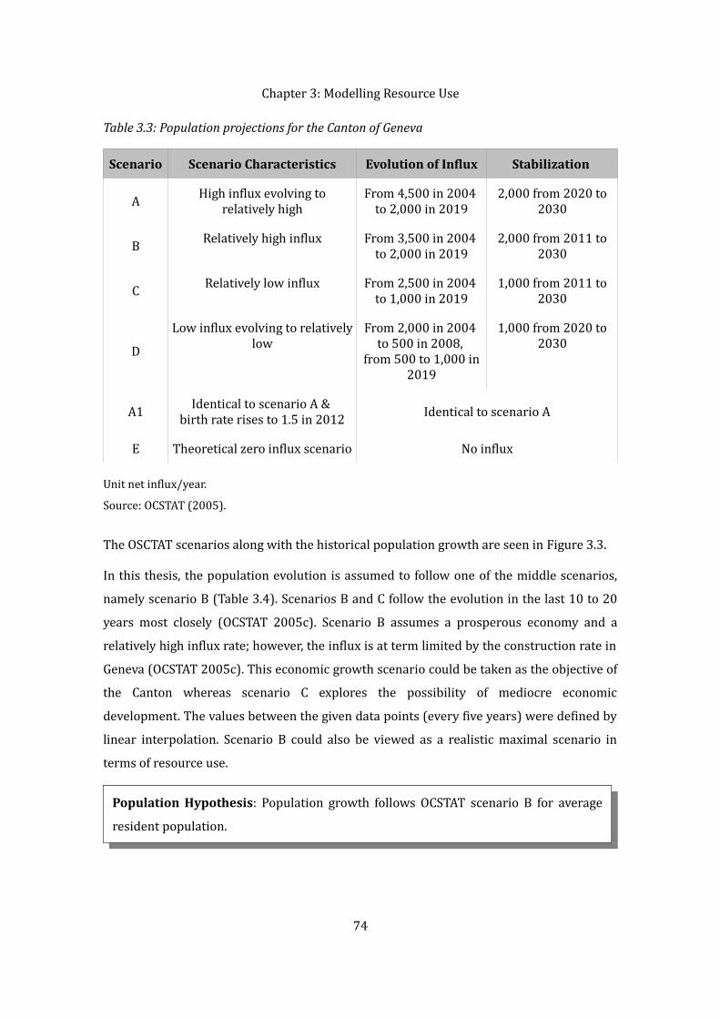
Chapter 3: Modelling Resource UseTable 3.3: Population projections for the Canton of Geneva

Scenario Scenario Characteristics Evolution of Influx Stabilization A High influx evolving to relatively high From 4,500 in 2004 to 2,000 in 2019 2,000 from 2020 to 2030B Relatively high influx From 3,500 in 2004 to 2,000 in 2019 2,000 from 2011 to 2030C Relatively low influx From 2,500 in 2004 to 1,000 in 2019 1,000 from 2011 to 2030D Low influx evolving to relatively low From 2,000 in 2004 to 500 in 2008, from 500 to 1,000 in 2019

1,000 from 2020 to 2030A1 Identical to scenario A & birth rate rises to 1.5 in 2012 Identical to scenario AE Theoretical zero influx scenario No influx

Unit net influx/year.Source: OCSTAT (2005).The OSCTAT scenarios along with the historical population growth are seen in Figure 3.3.In this thesis, the population evolution is assumed to follow one of the middle scenarios, namely scenario B (Table 3.4). Scenarios B and C follow the evolution in the last 10 to 20 years most closely (OCSTAT 2005c). Scenario B assumes a prosperous economy and a relatively high influx rate; however, the influx is at term limited by the construction rate in Geneva (OCSTAT 2005c). This economic growth scenario could be taken as the objective of the Canton whereas scenario C explores the possibility of mediocre economic development. The values between the given data points (every five years) were defined by linear interpolation. Scenario B could also be viewed as a realistic maximal scenario in terms of resource use.

Population Hypothesis: Population growth follows OCSTAT scenario B for average resident population.

74

Chapter 3: Modelling Resource Use

Table 3.4: Population projection, scenario B for 2004–2030

Scenario B 2004 2005 2010 2015 2020 2025 2030Population 436,990 441,844 461,703 478,763 495,308 511,685 527,309Mean yearly population addition - 4,854 3,972 3,412 3,309 3,275 3,125Mean yearly growth rate - 1.1% 0.9% 0.7% 0.7% 0.7% 0.6%

Source: OCSTAT (2005).The evolution of apparent consumption (economic system inflows) is assumed to follow population growth. On the other hand, the amount of waste (economic system outflows) is in most cases thought to correspond to the inflows with a given delay or residence time. Thus, the outputs are also dependent on the population but with a given time lag. The

75

Source: OCSTAT (2005; 2011b).Figure 3.3: Population projections for 2004–2030

Chapter 3: Modelling Resource UseGeneva population from 1920s to the near future is shown in Figure 3.4. Historical population data (OCSTAT n.d.) is used to model past resource consumption, which influences the resource stocks currently present in the economy as well as the amount of end-of-life products discarded as waste.

Our dynamic MFA model is therefore almost a linear model, as the projected population growth follows a near-linear curve. This aspect is use d to justify the application of local sensitivity analysis where the system sensitivity is analysed only at one fixed point (for more information on uncertainty assessment, see Chapter 3.4). 76

Data from 1920 to 2003 is based on historical statistics and data from 2004 onwards is based on population projections, i.e. scenario B (values from 2031 to 2080 are a continuation of the 2025–2030 linear interpolation).Source: OCSTAT (2005, 2011b, n.d.).Figure 3.4: Geneva population from 1920 to 2080

Chapter 3: Modelling Resource Use3.3.4 Adapting the Model FrameworkThe dynamic MFA model framework defined in this chapter has been further developed and adapted to the individual case studies on copper, phosphorus, and wood. However, in this section the aim was to summarize the common, overarching characteristics and hypotheses. The system definitions were slightly different for each of the substances studied as well as the defined scenarios; however, all three case studies contained a ‘Business as Usual’ scenario. A sensitivity analysis was performed for the copper case study (Chapter 4) whereas in the phosphorus case study (Chapter 5) an uncertainty analysis was carried out. The uncertainty aspects are presented in more detail in Chapter 3.4. 3.3.5 Choice of Modelling ToolThe dynamic MFA models were in practice implemented in SCILAB (version 5.3.2), a free numerical computation software tool (Digiteo 2011). This modelling tool was chosen primarily for the liberty it offered in model definition: the model type, its structure, and its dynamic behaviour were in no manner limited by the modelling software. However, the tool itself was not the focal point of the modelling exercise and the same dynamic model could undoubtedly be implemented with other software tools. For instance, MATLAB would offer the same type of programming environment while in system dynamics software (such as STELLA, VENSIM, or POWERSIM) the model construction would be of a slightly different nature. Another graphical tool for modelling dynamic systems is provided by the MATLAB extension SIMULINK. Other more MFA-specific software such as SIMBOX (Eawag 2011) or UMBERTO (ifu Hamburg 2011) could also be used. The use of more specialized dynamic modelling software might perhaps facilitate the task of sensitivity and uncertainty analysis, which some software can perform in an automated manner for a given system. Nevertheless, the flexibility and the easy availability offered by SCILAB were judged more important. 3.4 Uncertainty AssessmentLimited knowledge of parameter sensitivity and data uncertainty is often the weakness of traditional MFA studies as well as dynamic MFA models. There is very little literature on the subject of uncertainty assessment in material flow analysis. However, a short 77

Chapter 3: Modelling Resource Useintroduction can be found in Cencic (2004). More information on data uncertainties in MFA studies and their implications and a review of data uncertainties and MFA can be found in the work of Danius and Burström (2001; 2002). It has been concluded that the uncertainty of MFA studies is often so great that the results should be presented as intervals (Danius 2002).As uncertainty is often not given the attention it deserves in the field of MFA, it is necessary to study the treatment of uncertainty in mathematical models in general and in the environmental field in particular. In the following sections, uncertainty issues—the types of uncertainty and the most commonly used methodologies for uncertainty assessment—are presented from a more general standpoint. 3.4.1 Different Types of UncertaintyUncertainty has been defined as ‘any deviation from the unachievable ideal of completely deterministic knowledge of the relevant system’ (Walker et al. 2003). Uncertainty in mathematical models can actually be characterized in terms of three characteristics: the location, level, and nature of uncertainty (Walker et al. 2003). These three aspects are presented below. 3.4.1.1 Location of UncertaintyThe location of uncertainty refers to the place where the uncertainty is located within the model (Walker et al. 2003). These locations can include (Walker et al. 2003):

– context or identified system boundaries– model uncertainty that can be decomposed into model structure uncertainty (related to the model variables and their relationships) and model technical uncertainty (related to the technical implementation of the model)– inputs or references (system data) and the external driving forces causing changes in the reference system– parameter uncertainty connected to model parameters– model outcome uncertainty or the accumulated uncertainty in the model outcome

78

Chapter 3: Modelling Resource Use3.4.1.2 Level of UncertaintyThe level of uncertainty can be conceived in terms of a spectrum ranging from (unachievable) deterministic knowledge to total ignorance (Walker et al. 2003):

– Statistical uncertainty represents uncertainty that can be treated with statistical tools.– Scenario uncertainty is related to the scenarios as an illustration of plausible futures; this implies making assumptions about future development that are often unverifiable and beyond statistical uncertainty.– Recognised ignorance represents fundamental uncertainty about the phenomena under study.– Total ignorance represents the opposite of determinism on the scale of uncertainty; it implies that we are unaware of the full extent of our ignorance.In general, when modellers talk about uncertainty they refer only to statistical uncertainty. One should, however, bear in mind that deeper kinds of uncertainty exist, which cannot be characterized satisfactorily in statistical terms.

3.4.1.3 Nature of UncertaintyThe nature of uncertainty refers to the fact that the uncertainty can be due to the imperfect state of human knowledge or to inherent variability in the human or natural system described (Walker et al. 2003). The nature of uncertainty can thus be divided into epistemic uncertainty and variability uncertainty. Epistemic uncertainty represents uncertainty stemming from the shadowy areas in our knowledge, which may eventually be lightened by research efforts (Walker et al. 2003). Variability uncertainty, on the other hand, denotes uncertainty due to inherent randomness, unpredictability of human behaviour, various social, cultural and economic phenomena as well as technological developments (Walker et al. 2003). 3.4.2 Methodologies for Uncertainty AssessmentDozens of different methodologies for uncertainty assessment exist, each focusing on somewhat different locations and levels of uncertainty. Uncertainty assessment methods include for instance data uncertainty engine (DUE), error propagation equations, expert elicitation, extended peer review, inverse modelling (parameter estimation and predictive

79

Chapter 3: Modelling Resource Useuncertainty), Monte Carlo analysis, multiple model simulation, NUSAP, quality assurance, scenario analysis, sensitivity analysis, stakeholder involvement, and uncertainty matrix (Refsgaard et al. 2007). A more detailed presentation of these methodologies and their classification can be found in Refsgaard et al. (2007). Uncertainty in mathematical models is traditionally analysed from two different perspectives: the uncertainty in the model parameters is studied through sensitivity analysis and uncertainty in reference data is analysed via uncertainty analysis. These two approaches are presented briefly below. However, both tools cover only a limited range in the uncertainty location/level classification because we are dealing with statistical reference system and parameter uncertainty. The nature of uncertainty can be both epistemic and variable.3.4.2.1 Sensitivity AnalysisSensitivity analysis examines the influence of individual parameters on system variables (Cencic 2004). Linear models can be studied with local sensitivity analysis (or differential analysis) where one parameter is modified at a time and the model sensitivity to this parameter variation is inspected. To measure the impacts of the parameter variation, it is possible to construct sensitivity indices (Baccini & Bader 1996):

– Absolute sensitivity can be expressed asY j X j X j

(3.1)– Relative sensitivity can be expressed asY j X j X j

1Y j

(3.2)– Absolute sensitivity per 100% can be expressed asY j X j X j

X j (3.3)– Relative sensitivity per 100% can be expressed asY j X j X j

X j

Y j(3.4)

80

Chapter 3: Modelling Resource UseThe absolute sensitivity represents the absolute change ΔYj in the variable Yj with respect to a given change in parameter Xj. The relative sensitivity represents the relative change ΔYj /Yj in variable Yj with respect to a change in variable Xj. The absolute sensitivity per 100% represents the absolute change ΔYj in the variable Yj with respect to a (fictitious) 100% change in parameter Xj. The relative sensitivity per 100% represents the relative change ΔYj /Yj in variable Yj with respect to a (fictitious) 100% change in variable Xj. When dealing with non-linear models, it is necessary to employ global sensitivity analysis methods such as sampling methods, methods based on emulators, or various variance-based methods. Differential analysis techniques may also be used but it should be noted that their results are only valid for a limited range of the output space. For more information on sensitivity analysis, see, for instance, Saltelli et al. (2004).3.4.2.2 Uncertainty AnalysisUncertainty analysis studies the propagation of uncertainties from the input data to the model results. One commonly employed uncertainty analysis method is error propagation which is based on the Gauss’s error propagation equations. However, this method should only be employed when the variables are normally distributed and the uncertainties are small. When these conditions cannot be satisfied, Monte Carlo methods are often employed; in this case, it is necessary to have knowledge of the probability distributions of the input parameters and the correlations between them. In the case of over-determined systems, it is also possible to use least-square fitting techniques.More information on uncertainty analysis can be found for instance in Morgan and Henrion (1990). 3.4.3 Uncertainty Assessment in the Dynamic MFA ModelIn this thesis, I have chosen to perform a sensitivity analysis on the copper model (see Chapter 4.2.6) and an uncertainty analysis on the phosphorus model (Chapter 5.5). In the copper model, a local sensitivity analysis method has been used as the dynamic MFA model is nearly linear. This sensitivity analysis is only performed for the ‘Business as Usual’ scenario as it is assumed that the results would be similar for the other scenarios. No sensitivity analysis is performed on the phosphorus or the wood model; however, as

81

Chapter 3: Modelling Resource Usethe models’ structures are quite similar to the copper model, it can be surmised that the results would also be comparable.As no information is available on the uncertainty intervals of the initial data of the case studies, it is somewhat difficult to analyse the propagation of uncertainties in the dynamic simulations. It would be necessary to establish plausible uncertainty ranges for the initial MFA data. In the copper case study, the initial values of the dynamic simulation were based on a metabolism study done in the Canton of Geneva (Faist Emmenegger & Frischknecht 2003). However, no data uncertainties were given although the sources used to establish the data were of quite diverse natures. In the phosphorus case study, normalized data from a Swiss metabolism study (FOEN 2009b) was used and although the initial study establishes uncertainty values, it was not clear whether and how they can be used at the Geneva level. Also in the wood case study the uncertainties of the initial data were not known. As it is difficult to perform a rigorous and a complete uncertainty analysis based on our incomplete data, a simple error propagation analysis has been performed in the phosphorus case study. This analysis aims to establish the limits of error or the maximal uncertainty in the model results. As the input data cannot be assumed to be normally distributed or independent, the Gauss’s error propagation equations do not apply and maximal uncertainty values have therefore been calculated. However, there are also other types of uncertainty in our dynamic MFA model framework. For instance, in addition to statistical uncertainty there is scenario uncertainty: are the established scenarios plausible and are their assumptions reasonable? We also come across recognised ignorance notably when it comes to the basic assumptions on system behaviour: will the future resource needs be determined by population growth, economic development, or technological evolutions? What will be the future availability of supply?There is also uncertainty from different model locations besides the input and parameter uncertainty: the model structure itself is uncertain and debatable as well as the established system boundaries. For instance, MFA models only focus on physical quantities and the economic aspects—which also play an important part in resource depletion—are left outside the scope of the model. There is also uncertainty in the model structure concerning the hypothesis that resource consumption per capita remains stable as well as the delay and leaching characteristics determining the waste outputs. 82

Chapter 3: Modelling Resource Use3.5 DiscussionIn this chapter, a dynamic MFA model framework was constructed with fairly simple assumptions and easily understandable dynamics based on stable per capita consumption. However, while simplicity is an advantage for comprehension and analysis, it can also have its downfalls especially with respect to complex real-life phenomena. Moreover, the hypotheses forming the basis of the dynamic MFA model framework could also be chosen differently. Here, I attempt to summarize the various modelling choices and model aspects that could be improved on or otherwise modified. The fundamental characteristics of the dynamic MFA model include the following aspects:

– The model is a black-box model at the process level: it does not detail the internal complexity of the various processes of the system. – The environmental impacts of resource use are not taken into account.– The model framework deals only with stocks and flows of goods and substances in terms of physical units, no economic factors are taken into account.These three points are characteristic of material flow analyses, which focus on the physical stocks and flows of materials serving as inputs and outputs of processes identified inside a system of interest. Nevertheless, when studying phenomena related to resource depletion, it might be interesting to include commodity prices in the analysis since they are (at least to some degree) indicators of the rarity of the resource and influence its consumption. However, as I have chosen to work with MFA models, these economic factors are left outside the scope of the analysis. The model is a black-box model at the process level: it does not examine in detail the functioning of various subsystems. For instance, the agricultural subsystem encloses complex issues such as the efficiency of phosphorus fertilizers and the evolution of soluble and insoluble forms of phosphorus compounds in the soil. As phosphorus chemistry in the soil is quite complex, it is also difficult to evaluate the true residence time distribution of phosphorus. As regards the basic modelling hypotheses, the following choices could be discussed:– Resource consumption is determined solely by the population size. – No difference is made between product replacement sales and new sales.

83

Chapter 3: Modelling Resource Use– The relative importance of different economic sectors is assumed to stay constant.– The residence time of a material is determined for an entire economic sector at a time; there are no different product categories with different lifespans or lifespan distributions.– Technological improvements (e.g. in production or waste treatment) are not taken into account.In the dynamic MFA model, resource consumption is determined by the population size. This assumption seems logical when the goal is to predict the consumption of households but it might not apply to other economic sectors. However, it is easier to predict the evolution of the population than that of Geneva’s economy. For this reason, it is also assumed that the weight of the different economic sectors remains at the status quo.One of the shortcomings of the model framework is that no difference is made between new sales and replacement sales which often follow an entirely different logic. This aspect causes some particularities in the model behaviour: for instance, the increase in residence time has no influence on the predicted consumption, although in reality replacement sales should decrease. This phenomenon has no importance in the context of yearly renewed phosphate fertilizers or wood used as fuel; however, replacement sales do play a role in the case of copper used in consumer electronics or home appliances. The replacement versus new sales issue is closely linked to the difference between stock-based and flow-driven dynamic models.Instead of establishing an average residence time for an entire economic sector, it would also be more accurate to establish different product categories with their own lifespans. However, as our analysis is at a more global level, it is not certain that this would greatly contribute to the overall results. Another potential shortcoming of the model is that any technological improvements are not taken into account for instance in terms of the improvement of recycling rates or material use efficiency. However, as it is notoriously difficult to make predictions about future technological development, this aspect has been eliminated from the scope of the analysis.

84

Chapter 3: Modelling Resource UseIn addition to the model and its assumptions, it should also be remembered that the initial data used in the dynamic analysis as well as the model parameter values are of great importance. Any analysis can only be as good as the underlying data.3.6 ConclusionIn this chapter, the framework for a dynamic MFA model was laid out. The proposed model is driven by population growth; it is assumed that the per capita consumption stays constant. The waste flows are assumed to be determined by a delay process except in the agricultural sector of the phosphorus case study (Chapter 5) where there is a leaching-type process. The dynamic MFA model framework can now be applied to our case studies in the Canton of Geneva and be used to create customized models for each material studied.

85

Thesis Structure

PART IIICASE STUDIES AND MODEL

CONSTRUCTION

88

Chapter 4: Case Study on Copper Chapter 4 Case Study on Copper 4.1 IntroductionThis chapter begins by presenting the main uses and characteristics of copper followed by an introduction to copper metabolism in the Canton of Geneva. A dynamic MFA model for copper is constructed in Chapter 4.2 and the world copper production is analysed in Chapter 4.3. The sustainability of copper use is studied via an autarky indicator in Chapter 4.4 using information from both the dynamic MFA model and the predictions on world copper production. Discussions and a conclusion are provided in Chapters 4.5 and 4.6. 4.1.1 The Uses and Characteristics of CopperCopper is one of the most important metals in the world today (third after iron and aluminium in terms of weight) as well as one of the oldest, dating back 7000 years (Radetzki 2009). Due to the metal’s importance, copper metabolism has been studied widely (examples of studies include, for instance, Ayres et al. 2002; Spatari et al. 2002; Graedel et al. 2004; Spatari et al. 2005; Gordon et al. 2006). Copper’s chemical, physical, and aesthetic properties (such as malleability, ductility, conductivity of heat and electricity, and corrosion resistance) make it widely used in a large range of industrial, domestic, and high technology applications such as telecommunications, construction, and transportation as well as in various electrical and electronic devices (Radetzki 2009). As a micronutrient and essential trace element, copper is vital to humans, animals, and plants (ICSG 2009). Even though substitution in favour of aluminium, steel, plastics, and optical fibre could reduce copper demand, it is hard to conceive how modern society could cope without a large-scale secure copper supply (ICSG 2007; Radetzki 2009). Indeed, copper consumption has increased on average by 4% a year since 1900 (ICSG 2009). Copper can be recycled without losing any of its properties and it is currently among the most recycled metals: in 2007, about 35% of copper consumption came from recycled copper (ICSG 2009). Besides primary copper deposits, anthropogenic copper stocks are of increasing importance; it has been estimated that during the 20 th century about 40% of the copper consumed in North America was stored as in-use stock while over 30% was lost as dissipated or landfilled waste (Spatari et al. 2005).

89

Chapter 4: Case Study on Copper Copper is sometimes referred to as ‘Dr. Copper’ since it provides a good indicator of overall economic activity level due to its wide usage in society (see, for instance, La Monica 2011). Copper prices increased greatly (nearly quintupling) from 2000 to 2008 (ICSG 2009). Although the prices have fallen as a result of the current economic crisis, they are expected to increase in the future as a result of ever-growing demand in China and in other developing countries. Copper reserves are estimated at 550 Mt (USGS 2009); this would provide a reserves-to-production ratio of about 36 years with the global production levels of 2008, or 15.4 Mt (USGS 2010a). In this case study, copper was chosen as the resource of interest for several reasons: firstly, it is an important and widely-used resource in the world today and, secondly, the current copper reserves could be depleted in the course of a few decades (18–28 years) (OECD 2008c). (For more information on peak copper, see Chapter 4.3.) In addition, an existing study of copper metabolism in the Canton of Geneva (Faist Emmenegger & Frischknecht 2003) provides a starting point for our analysis. 4.1.2 Copper Metabolism in the Canton of GenevaCopper metabolism in the Canton of Geneva has already been studied in a substance flow analysis for the year 2000 (Faist Emmenegger & Frischknecht 2003). The copper use in different economic sectors according to this study is shown in Table 4.1. The greatest copper flows in the Canton are related to buildings (in the primary and tertiary sectors and in households) and to industrial use (in the secondary sector). The primary sector includes agriculture, forestry and extractive activities while the secondary sector consists of construction and manufacturing industries as well as of electricity, gas and water utilities. The tertiary sector includes transport, services, and various commercial activities. For more information, see Faist Emmenegger and Frischknecht (2003). As copper use in buildings is one of the substance’s most important applications, it is interesting to take a closer look at this domain. Copper use in buildings in Switzerland has been studied by Wittmer (2006): roofing and guttering are responsible for 41% of copper contained in buildings, followed by electric and heating installations, at 30% and 17% respectively (Table 4.2).

90

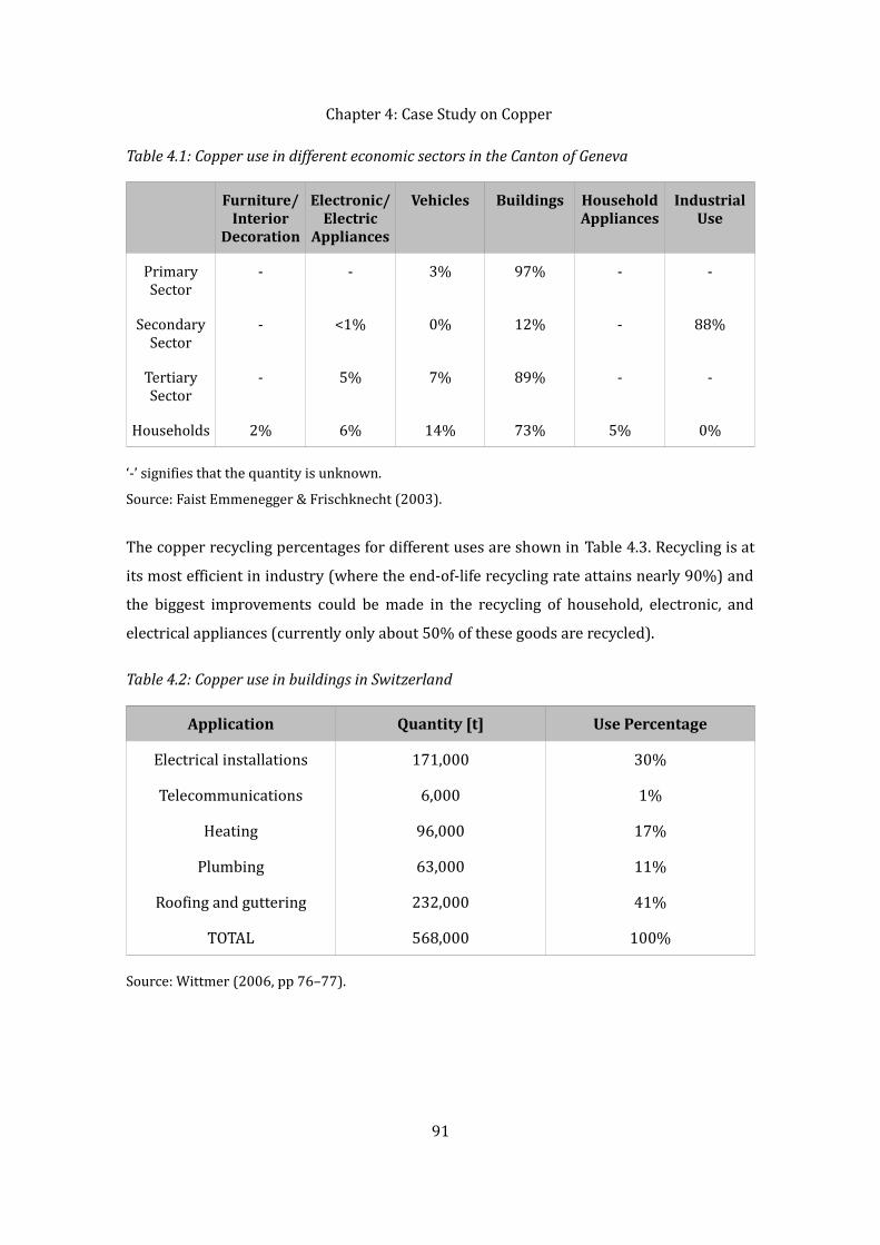
Chapter 4: Case Study on Copper Table 4.1: Copper use in different economic sectors in the Canton of Geneva

Furniture/ Interior

Decoration

Electronic/Electric

Appliances

Vehicles Buildings Household Appliances

Industrial Use

Primary Sector - - 3% 97% - -Secondary Sector - <1% 0% 12% - 88%

Tertiary Sector - 5% 7% 89% - -Households 2% 6% 14% 73% 5% 0%

‘-’ signifies that the quantity is unknown. Source: Faist Emmenegger & Frischknecht (2003). The copper recycling percentages for different uses are shown in Table 4.3. Recycling is at its most efficient in industry (where the end-of-life recycling rate attains nearly 90%) and the biggest improvements could be made in the recycling of household, electronic, and electrical appliances (currently only about 50% of these goods are recycled). Table 4.2: Copper use in buildings in Switzerland

Application Quantity [t] Use PercentageElectrical installations 171,000 30%Telecommunications 6,000 1%Heating 96,000 17%Plumbing 63,000 11%Roofing and guttering 232,000 41%TOTAL 568,000 100%Source: Wittmer (2006, pp 76–77).

91

Chapter 4: Case Study on Copper Table 4.3: Copper recycling in the Canton of Geneva

Application Total Quantity [t] Recycling PercentageFurniture 20 75%Electronic/electrical appliances 130 50%Vehicles 220 80%Buildings 2,100 75%Household appliances 40 51%Industrial use 1,900 88%TOTAL 4,500 79%*

*The average global recycling percentage. The total quantity represents the quantity of copper consumed in the Canton of Geneva without addition to stock and exports.Source: Faist Emmenegger & Frischknecht (2003). 4.2 Dynamic Modelling of Copper Metabolism in the Canton of Geneva4.2.1 Copper Metabolism in Geneva in 2000The data presented here are based on a metabolism study for the year 2000 (Faist Emmenegger & Frischknecht 2003). The results of this study in terms of copper are summarized in Figure 4.1. There are no copper mines nor refineries in the Canton of Geneva and all the copper consumed in the Canton must therefore be imported. About 81% of copper waste was recycled in 2000 while the rest was landfilled. Copper recycling takes place outside the Canton and all the copper scrap is therefore exported. The amount of recycled copper corresponds to 53% of net copper imports.

92

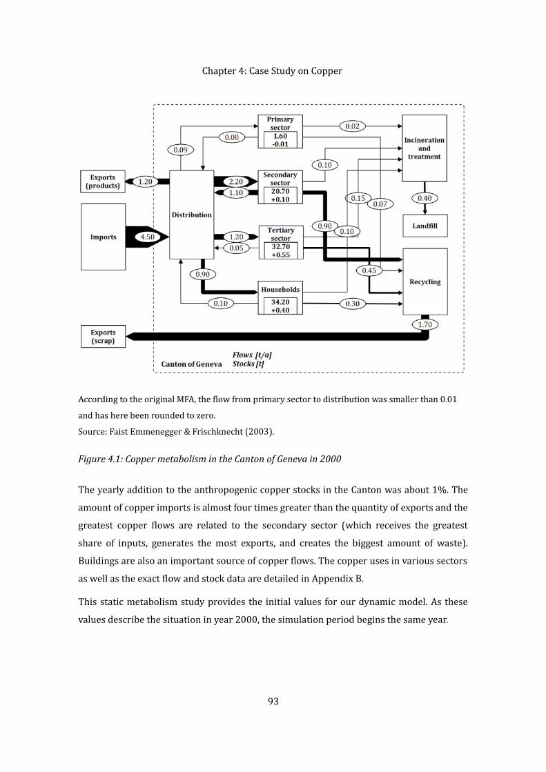
Chapter 4: Case Study on Copper

The yearly addition to the anthropogenic copper stocks in the Canton was about 1%. The amount of copper imports is almost four times greater than the quantity of exports and the greatest copper flows are related to the secondary sector (which receives the greatest share of inputs, generates the most exports, and creates the biggest amount of waste). Buildings are also an important source of copper flows. The copper uses in various sectors as well as the exact flow and stock data are detailed in Appendix B. This static metabolism study provides the initial values for our dynamic model. As these values describe the situation in year 2000, the simulation period begins the same year.

93

According to the original MFA, the flow from primary sector to distribution was smaller than 0.01 and has here been rounded to zero.Source: Faist Emmenegger & Frischknecht (2003). Figure 4.1: Copper metabolism in the Canton of Geneva in 2000

Chapter 4: Case Study on Copper 4.2.2 Stock and Flow Model for Copper MetabolismBased on the representation of the year 2000 SFA, a stock and flow model for the copper metabolism in Geneva was defined (Figure 4.2). The state equations of the defined system are presented in Appendix B. This model is only a representation of the interconnected stocks and flows of the system; we have no knowledge yet of the forces driving the system behaviour.

The stocks and flows of the system have been named as Si and fi. The processes (subsystems) are detailed in Table 4.4. The changes in stock in the import and export processes are not examined since they are outside the system limits (marked by a dashed line). There is no material accumulation in the processes ‘Distribution’, ‘Incineration and treatment’ and ‘Recycling’, the inputs of these processes are always equal to the outputs.94

Source: system representation adapted from Faist Emmenegger & Frischknecht (2003).Figure 4.2: Stock and flow model for copper metabolism in the Canton of Geneva

Chapter 4: Case Study on Copper Table 4.4: Copper system processes

Process Name Process Description Change in StockImports Import of copper containing goods from outside the Canton -

Exports (products) Exports of copper containing goods (including used cars) -Distribution Distribution of copper containing goods to the economic sectors No

Primary Sector Use of copper in the primary sector YesSecondary Sector Use of copper in the secondary sector (industry) YesTertiary Sector Use of copper in the tertiary sector (services) YesHouseholds Use of copper in households YesIncineration and Treatment Incineration and treatment of copper containing waste NoLandfills Landfilling of copper containing waste YesRecycling Collection of copper containing waste NoExports (recycled materials) Export of copper containing waste to be recycled outside the Canton -

Source: adapted from Faist Emmenegger & Frischknecht (2003).The stock and flow model has in total 30 unknown variables:

– 20 flows– 5 stocks – 5 changes in stock30 equations are therefore needed to solve the system (see Appendix B for details).

4.2.3 Precision on Vocabulary and Basic HypothesesSome precisions on the vocabulary used: – Net imports (as well as apparent copper consumption) correspond to f1 – f2.

95

Chapter 4: Case Study on Copper – The amount of copper recycled outside the Canton corresponds to the flow f20; the recycled copper can later be used as secondary copper.– The amount of primary copper required is defined as the difference of net imports and recycled copper, f1 – f2 – f20.It should be noted that this thesis concentrates on resource use in the Canton (apparent consumption); the amount of exported copper products is thus not analysed in detail. Any possible losses in copper scrap processing are not taken into account. It is assumed that although the recycled copper collected in the Canton is recycled outside its borders, it could be used to provide for a part of the copper needs in the Canton thus diminishing the required amount of primary copper. While secondary copper provides for a part of the Canton’s resource needs, it is assumed that the remaining part is satisfied by primary copper resources, although in reality there is no information on the exact nature (primary/secondary) of the copper imports.

4.2.4 Dynamic Behaviour of the SystemIn order to explore different potential evolutions in the system, several scenarios have been defined. The scenarios examined were (Table 4.5):– Business as Usual– 90% Recycling of Building Waste– Substitution in Roofing and Guttering– Electric Mobility– No Primary Copper ConsumptionThe ‘Business as Usual’ scenario is seen as a continuation of the current tendencies whereas the other three scenarios reflect possible changes in the system behaviour. ‘90% Recycling of Building Waste’ is a scenario exploring the benefits of improved building waste recycling: the current recycling rate of 75% (Faist Emmenegger & Frischknecht 2003) is expected to rise to 90%. The scenarios ‘Substitution in Roofing and Guttering’ and ‘Electric Mobility’ describe changes in the copper consumption per capita: in this electric mobility scenario, net imports per capita are assumed to rise to 8.3 kg/year whereas in the substitution scenario the net imports per capita decline to 5.8 kg/year. The ‘No Primary

96

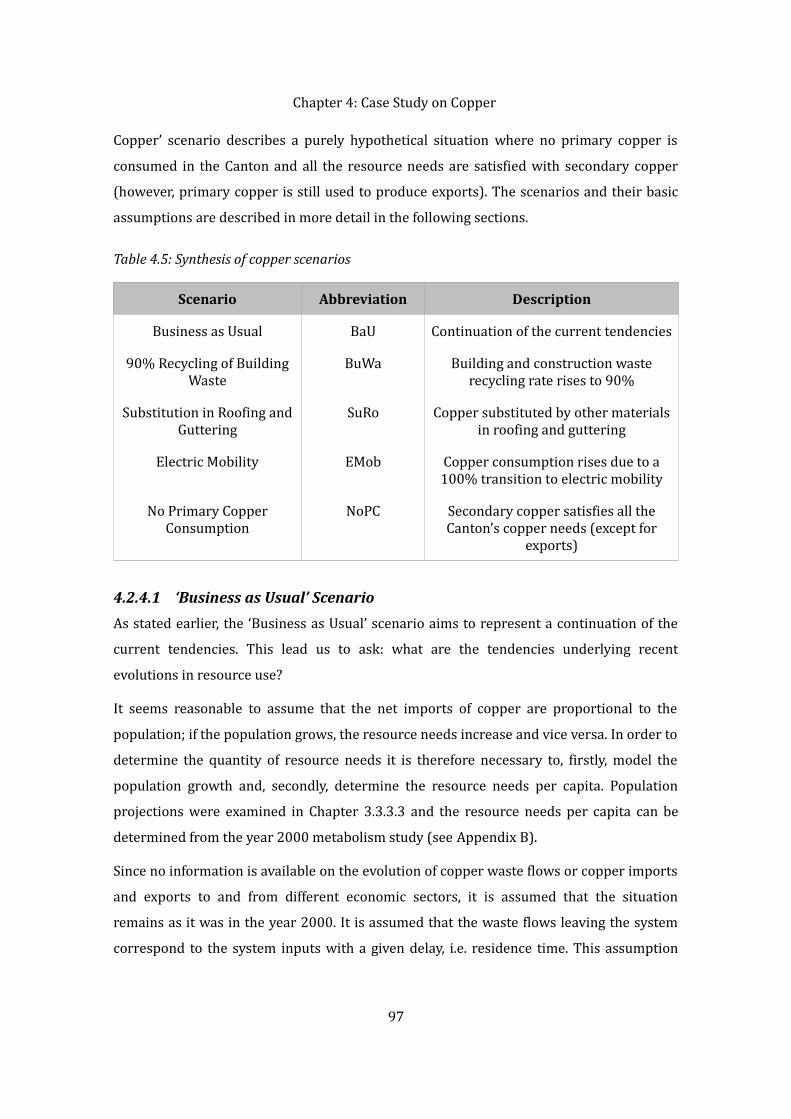
Chapter 4: Case Study on Copper Copper’ scenario describes a purely hypothetical situation where no primary copper is consumed in the Canton and all the resource needs are satisfied with secondary copper (however, primary copper is still used to produce exports). The scenarios and their basic assumptions are described in more detail in the following sections. Table 4.5: Synthesis of copper scenarios

Scenario Abbreviation DescriptionBusiness as Usual BaU Continuation of the current tendencies90% Recycling of Building Waste BuWa Building and construction waste recycling rate rises to 90%Substitution in Roofing and Guttering SuRo Copper substituted by other materials in roofing and gutteringElectric Mobility EMob Copper consumption rises due to a 100% transition to electric mobilityNo Primary Copper Consumption NoPC Secondary copper satisfies all the Canton’s copper needs (except for exports)4.2.4.1 ‘Business as Usual’ ScenarioAs stated earlier, the ‘Business as Usual’ scenario aims to represent a continuation of the current tendencies. This lead us to ask: what are the tendencies underlying recent evolutions in resource use? It seems reasonable to assume that the net imports of copper are proportional to the population; if the population grows, the resource needs increase and vice versa. In order to determine the quantity of resource needs it is therefore necessary to, firstly, model the population growth and, secondly, determine the resource needs per capita. Population projections were examined in Chapter 3.3.3.3 and the resource needs per capita can be determined from the year 2000 metabolism study (see Appendix B).Since no information is available on the evolution of copper waste flows or copper imports and exports to and from different economic sectors, it is assumed that the situation remains as it was in the year 2000. It is assumed that the waste flows leaving the system correspond to the system inputs with a given delay, i.e. residence time. This assumption

97

Chapter 4: Case Study on Copper indicates a situation where consumed copper goods are used during a certain time and then discarded as waste. The basic hypotheses with regard to the dynamic behaviour of the baseline scenario can now be formulated in the following manner:1. Net imports f1(t) – f2(t) remain proportional to the population p(t). In simpler terms, it is assumed that copper imports and exports (of copper products) are proportional to the population size; as a result of this assumption, net imports also remain proportional to population. This assumption is made in order to simplify the analysis; our focus is on the evolution of (apparent) copper use in Geneva and the development of exports is of lesser interest. Moreover, it is difficult to predict the development of copper exports as this depends on the global economic situation and not only on the economy and industry in Geneva. One could also argue that the exports are correlated with the population since both depend on the economic situation: a good economic situation in the Canton could be surmised to draw more migrants looking for work. 2. The net imports per capita remains at the year 2000 level, or 7.9 kg per capita per year (Faist Emmenegger & Frischknecht 2003). According to historical data, net copper imports per capita have varied between approximately 5–12 kg per capita since the 1960s (Wittmer 2006). The value of 7.9 kg seems therefore fairly average. However, the net imports per capita were somewhat lower in the 1950s (about 3 kg/year/inhabitant); this might cause some errors in the simulation as the simulated amount of waste should exceed the real values for the oldest waste.3. The relative sizes of import and export flows remain unchanged with respect to the year 2000.4. The percentages of recycled and landfilled waste remain unchanged.5. The outflows from the economic sectors correspond to the inflows with a given delay (i.e. residence time); each of the four sectors has its own characteristic residence time.The copper residence times for different sectors were estimated using data from two sources: Spatari et al. (2005) and Van Beers et al. (2007). The residence times are 98

Chapter 4: Case Study on Copper summarized in Table 4.6; a more detailed explication of their calculation and sources is provided in Appendix B.Table 4.6: Copper residence times

Economic Sector Estimated Residence TimePrimary Sector 44Secondary Sector 26Tertiary Sector 43Households 37

4.2.4.2 ‘90% Recycling of Building Waste’ ScenarioThe recycling scenario is based on the rules defined for the baseline scenario with one important distinction: it is assumed that the recycling rate of building waste shall rise from the current 75% (Faist Emmenegger & Frischknecht 2003) to 90%. The transition is assumed to take place gradually during 2010–2020. The recycling rate in industry is already close to 90% (Faist Emmenegger & Frischknecht 2003) and it is therefore possible to assume that the same rate could be obtained in building waste recycling. The basic hypotheses of the recycling scenario can now be formulated in the following manner:1. Rules 1–3 and 5 from the previously defined ‘Business as Usual’ scenario apply.2. The following rules apply to recycled and landfilled waste:• Before 2010,the situation is as in 2000 (‘Business as Usual’ rule 4 applies).• Between 2010 and 2020, the building waste recycling percentage increases in a linear manner.• After 2020, 90% of building waste is recycled, increasing the overall copper recycling rate to about 89%.The copper flows resulting from this increased recycling are detailed in Appendix B.

99

Chapter 4: Case Study on Copper 4.2.4.3 ‘Substitution in Roofing and Guttering’ ScenarioThe substitution scenario is also based on the baseline scenario rules with a change concerning net imports per capita, which are assumed to diminish during 2010–2020 to a level of about 5.8 kg/year/inhabitant. Per capita copper needs therefore decrease by almost 30% from the year 2000 level. This scenario corresponds to the substitution of copper in roofing and guttering where it represents 41% of copper use in buildings (Wittmer 2006). Roofing and guttering is one of the areas in which copper usage could be quite easily replaced. Copper could be substituted for instance with zinc, aluminium, or composite copper sheet (ICSG 2007). However, the use of copper in facing and roofing remains popular, despite its high cost as compared with alternatives such as aluminium, galvanized iron, and various other materials (Ayres et al. 2002). This stems from the advantages of long life, recyclability, and low maintenance, as well as aesthetic values (Ayres et al. 2002). Decreasing copper use in roofing and guttering would also help to slow down dissipation as the corrosion of copper roofs and copper pipes can be a major source of anthropogenic copper dissipation in the environment (Ayres et al. 2002).The basic hypotheses of the substitution scenario can now be formulated in the following manner:1. Rules 1 and 4–5, previously defined for the ‘Business as Usual’ scenario, apply.2. The apparent consumption per capita follows the following trajectory:

• Before 2010, net imports per capita remain at the year 2000 level (‘Business as Usual’ rule 2). • From 2010 to 2020, net imports per capita decrease linearly as copper is substituted in roofing and guttering by other materials. The reduction in each economic sector is determined by its copper use in buildings. • After 2020, all the copper in roofing and guttering has been substituted and the net imports per capita are approximately 5.8 kg/year. The copper flows after substitution are detailed in Appendix B.

100

Chapter 4: Case Study on Copper 4.2.4.4 ‘Electric Mobility’ ScenarioThe e-mobility scenario reflects a more copper-intensive future, resulting from increased copper use in electric mobility: per capita copper needs increase to 8.3 kg/year/inhabitant, which corresponds to about a 5% increase from the year 2000 level. The net imports per capita are assumed to grow linearly during 2010–2020 to attain the aforementioned level. It is estimated that the copper use in vehicles in 2020 shall be twice the current amount. This increase is thought to stem from the replacement of internal combustion engine (ICE) vehicles with electric vehicles (EVs). The amount of copper used in EVs has been estimated to be double the amount of copper used in vehicles based on internal combustion (Weed 1998). The amount of existing electric vehicles in 2000 is not taken into account as it is assumed to be very small compared to non-electric ones.The basic hypotheses of the e-mobility scenario can now be formulated in the following manner:1. Rules 1 and 4–5 from the previously defined ‘Business as Usual’ scenario apply.2. Net imports per capita follow the following trajectory:

• Before 2010, net imports remain at the 2000 level (‘Business as Usual’ rule 2).• From 2010 to 2020, net imports increase linearly. The increase in each economic sector is determined by its copper use in vehicles. • After 2020, the transition to electric mobility is complete and the net imports are at approximately 8.3 kg/year/inhabitant.The copper flows resulting from increased e-mobility are detailed in Appendix B.

4.2.4.5 ‘No Primary Copper Consumption’ ScenarioThe ‘No Primary Copper’ scenario reflects a purely hypothetical situation where the primary copper consumption is zero and only secondary copper is consumed in the Canton of Geneva. In this situation, there would be no dependency on external copper sources that could be disrupted either for geopolitical or for geological scarcity reasons. (However, we should bear in mind that secondary copper is refined outside the Canton.) As in the other scenarios, it is assumed that the transition to this new state takes place gradually from 2010 to 2020; the secondary copper use rate is thus 100% from 2020 onwards.101

Chapter 4: Case Study on Copper The basic hypotheses of the ‘No Primary Copper’ scenario can now be formulated in the following manner:1. Rules 2–5, previously defined for the ‘Business as Usual’ scenario, apply.2. The following rules apply to copper consumption:• Before 2010, the situation is as in 2000 (‘Business as Usual’ rule 1 applies).• Between 2010 and 2020, the primary copper consumption decreases to zero in a linear manner.• After 2020, the usage rate of secondary copper is 100% and primary copper stands at 0%; copper recycling represents the only copper source in the Canton of Geneva. It is assumed that exports are still produced using primary copper imports; however, their quantity declines in pace with the cantonal consumption.If the exports were also assumed to be produced using secondary copper, the primary copper needs in the Canton (as they are defined in Chapter 4.2.3) would actually become negative as recycled copper is also used to provide exports. The exports are here assumed to decline in the same manner as copper consumption in the Canton (i.e. secondary copper imports) as a result of a decrease in industry focused on copper products.

4.2.5 Model Results

4.2.5.1 Presentation of Model ResultsAfter constructing the dynamic MFA model, it is now possible to use this model to simulate the copper metabolism in the Canton of Geneva in the coming decades. The evolution of apparent copper consumption (inputs of the system) is assumed to follow population growth. On the other hand, the amount of wastes (system outflows) is thought to correspond to the economic system inflows with a given delay or residence time. The simulations were performed for the time period 2000–2080. This time period was chosen in order to clearly see the evolutions taking place at the recycling and waste creation end of the system considering the various residence times (from 26 to 44 years) and scenarios (resource use evolutions taking place from 2010 to 2020). A longer time period was not inspected since a population projection is only available until 2030 and the values beyond this point must thus be estimated. 102

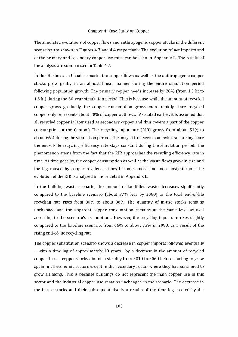
Chapter 4: Case Study on Copper The simulated evolutions of copper flows and anthropogenic copper stocks in the different scenarios are shown in Figures 4.3 and 4.4 respectively. The evolution of net imports and of the primary and secondary copper use rates can be seen in Appendix B. The results of the analysis are summarized in Table 4.7.In the ‘Business as Usual’ scenario, the copper flows as well as the anthropogenic copper stocks grow gently in an almost linear manner during the entire simulation period following population growth. The primary copper needs increase by 20% (from 1.5 kt to 1.8 kt) during the 80-year simulation period. This is because while the amount of recycled copper grows gradually, the copper consumption grows more rapidly since recycled copper only represents about 80% of copper outflows. (As stated earlier, it is assumed that all recycled copper is later used as secondary copper and thus covers a part of the copper consumption in the Canton.) The recycling input rate (RIR) grows from about 53% to about 66% during the simulation period. This may at first seem somewhat surprising since the end-of-life recycling efficiency rate stays constant during the simulation period. The phenomenon stems from the fact that the RIR approaches the recycling efficiency rate in time. As time goes by, the copper consumption as well as the waste flows grow in size and the lag caused by copper residence times becomes more and more insignificant. The evolution of the RIR is analysed in more detail in Appendix B.In the building waste scenario, the amount of landfilled waste decreases significantly compared to the baseline scenario (about 37% less by 2080) as the total end-of-life recycling rate rises from 80% to about 88%. The quantity of in-use stocks remains unchanged and the apparent copper consumption remains at the same level as well according to the scenario’s assumptions. However, the recycling input rate rises slightly compared to the baseline scenario, from 66% to about 73% in 2080, as a result of the rising end-of-life recycling rate.The copper substitution scenario shows a decrease in copper imports followed eventually—with a time lag of approximately 40 years—by a decrease in the amount of recycled copper. In-use copper stocks diminish steadily from 2010 to 2060 before starting to grow again in all economic sectors except in the secondary sector where they had continued to grow all along. This is because buildings do not represent the main copper use in this sector and the industrial copper use remains unchanged in the scenario. The decrease in the in-use stocks and their subsequent rise is a results of the time lag created by the 103

Chapter 4: Case Study on Copper copper residence times: when consumption initially diminishes, there are still abundant in-use copper stocks but when the old stocks are depleted, they are replaced by less in-use copper and the amount of recyclable copper thus diminishes in time. In the case of substitution, the net copper imports are almost 30% lower than in the baseline scenario and the recycled copper provides for about 80% of the needs in the Canton from 2020 to 2050. In-use copper stocks have diminished by about 31% by 2080. In the e-mobility scenario, copper flows and anthropogenic copper stocks increase slightly: the in-use stocks increase by 6% by 2080 and the net imports by 5% compared to the baseline scenario. The recycling input rate decreases slightly (from 80% to 79% in 2080). In general, the e-mobility scenario differs only slightly from the ‘Business as Usual’ scenario as the per capita copper consumption increases from 7.9 kg to 8.3 kg.According to the ‘No Primary Copper’ scenario’s assumptions, primary copper consumption in the Canton tends to hit zero after 2020 and secondary copper presents the only copper source. As only about 80% of copper waste is recycled (as opposed to 100%), the secondary copper inputs must diminish over time. However, this is only the general rule and in practice we can see for instance an increase from 2020 to 2030 as a delayed response to an increase in inputs driven by population growth. The in-use stocks start to decrease from 2020 onwards as a result of the decrease in net imports (over 60% less than in the baseline scenario by 2080). The stock of landfilled copper continues to grow although less than in the baseline scenario (18% less by 2080) since the inflow is smaller. The net imports per capita decrease to about 2.9 kg by 2080; this represents less than 40% of the ‘Business as Usual’ value.

104

Chapter 4: Case Study on Copper

105BaU = ‘Business as Usual’, BuWa = ‘90% Recycling of Building Waste’, SuRo = ‘Substitution in Roofing and Guttering’, EMob = ‘Electric Mobility’, NoPC = ‘No Primary Copper Consumption’.Figure 4.3: Simulated copper flows

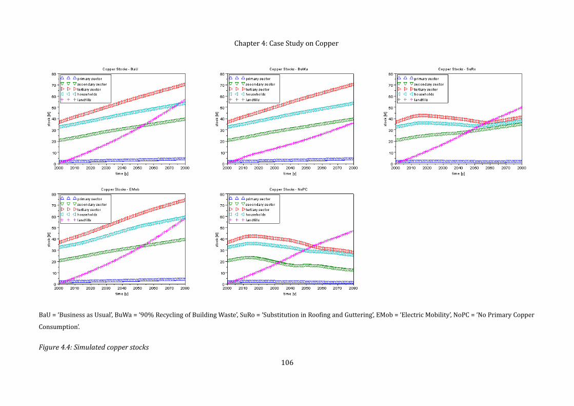
Chapter 4: Case Study on Copper

106BaU = ‘Business as Usual’, BuWa = ‘90% Recycling of Building Waste’, SuRo = ‘Substitution in Roofing and Guttering’, EMob = ‘Electric Mobility’, NoPC = ‘No Primary Copper Consumption’.Figure 4.4: Simulated copper stocks

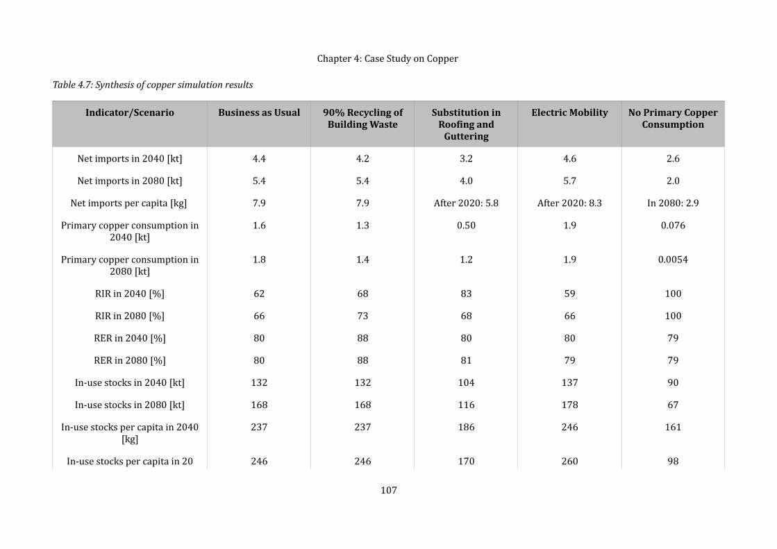
Chapter 4: Case Study on Copper Table 4.7: Synthesis of copper simulation results

Indicator/Scenario Business as Usual 90% Recycling of Building Waste

Substitution in Roofing and

Guttering

Electric Mobility No Primary Copper Consumption

Net imports in 2040 [kt] 4.4 4.2 3.2 4.6 2.6Net imports in 2080 [kt] 5.4 5.4 4.0 5.7 2.0Net imports per capita [kg] 7.9 7.9 After 2020: 5.8 After 2020: 8.3 In 2080: 2.9Primary copper consumption in 2040 [kt] 1.6 1.3 0.50 1.9 0.076Primary copper consumption in 2080 [kt] 1.8 1.4 1.2 1.9 0.0054

RIR in 2040 [%] 62 68 83 59 100RIR in 2080 [%] 66 73 68 66 100RER in 2040 [%] 80 88 80 80 79RER in 2080 [%] 80 88 81 79 79In-use stocks in 2040 [kt] 132 132 104 137 90In-use stocks in 2080 [kt] 168 168 116 178 67In-use stocks per capita in 2040 [kg] 237 237 186 246 161In-use stocks per capita in 20 246 246 170 260 98

107

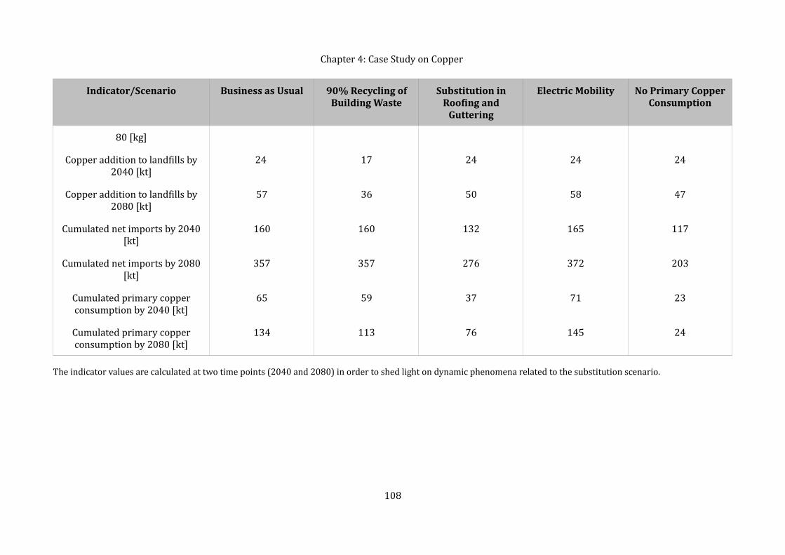
Chapter 4: Case Study on Copper Indicator/Scenario Business as Usual 90% Recycling of

Building WasteSubstitution in

Roofing and Guttering

Electric Mobility No Primary Copper Consumption

80 [kg]Copper addition to landfills by 2040 [kt] 24 17 24 24 24Copper addition to landfills by 2080 [kt] 57 36 50 58 47

Cumulated net imports by 2040 [kt] 160 160 132 165 117Cumulated net imports by 2080 [kt] 357 357 276 372 203

Cumulated primary copper consumption by 2040 [kt] 65 59 37 71 23Cumulated primary copper consumption by 2080 [kt] 134 113 76 145 24

The indicator values are calculated at two time points (2040 and 2080) in order to shed light on dynamic phenomena related to the substitution scenario.

108

Chapter 4: Case Study on Copper 4.2.5.2 Confrontation of Model ResultsThe waste flows predicted by the simulation model and the ones observed in the year 2000 metabolism study are compared in Table 4.8. It is clear that in order to obtain a more accurate estimation of the wastes of each economic sector, it would be necessary to model the sectors’ past and future development. It is for instance possible that the copper consumption of the primary sector was greater in the past than it is at present and that the tertiary sector and households consumed less copper than currently. However, on a global level, our dynamic MFA model performs relatively accurately: the differences in the aggregated landfilled and recycled waste flows for the year 2000 are respectively 4% and 9%. Table 4.8: Comparison of simulated and reference waste flows in 2000

Waste Flow Value According to Model [kg]

Value According to Metabolism Study [kg]Landfilled waste S1 12 24Landfilled waste S2 90 95Landfilled waste S3 174 156Landfilled waste HH 164 128TOTAL 440 402

Recycled waste S1 35 71Recycled waste S2 829 876Recycled waste S3 504 453Recycled waste HH 430 335TOTAL 1798 1736S1 = primary sector, S2 = secondary sector, S3 = tertiary sector, HH = households.Source: the values of the metabolism study are from Faist Emmenegger & Frischknecht (2003).

109

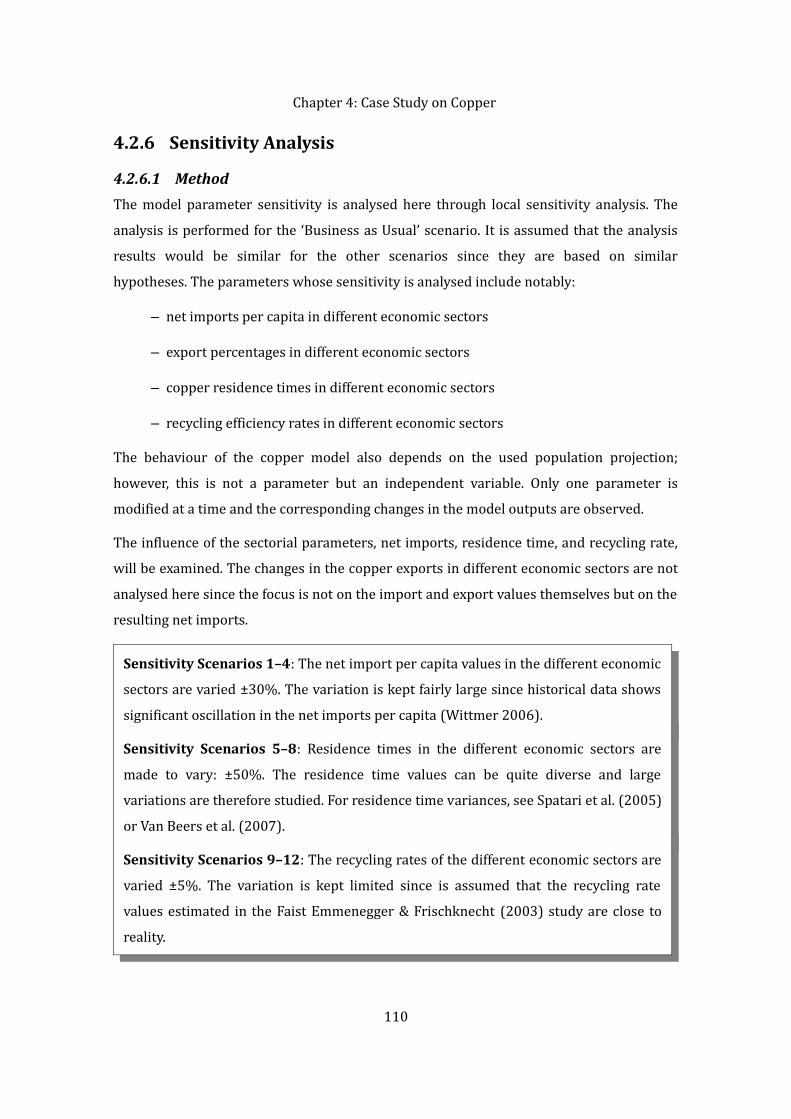
Chapter 4: Case Study on Copper 4.2.6 Sensitivity Analysis

4.2.6.1 MethodThe model parameter sensitivity is analysed here through local sensitivity analysis. The analysis is performed for the ‘Business as Usual’ scenario. It is assumed that the analysis results would be similar for the other scenarios since they are based on similar hypotheses. The parameters whose sensitivity is analysed include notably:– net imports per capita in different economic sectors– export percentages in different economic sectors– copper residence times in different economic sectors– recycling efficiency rates in different economic sectorsThe behaviour of the copper model also depends on the used population projection; however, this is not a parameter but an independent variable. Only one parameter is modified at a time and the corresponding changes in the model outputs are observed.The influence of the sectorial parameters, net imports, residence time, and recycling rate, will be examined. The changes in the copper exports in different economic sectors are not analysed here since the focus is not on the import and export values themselves but on the resulting net imports.

Sensitivity Scenarios 1–4: The net import per capita values in the different economic sectors are varied ±30%. The variation is kept fairly large since historical data shows significant oscillation in the net imports per capita (Wittmer 2006). Sensitivity Scenarios 5–8: Residence times in the different economic sectors are made to vary: ±50%. The residence time values can be quite diverse and large variations are therefore studied. For residence time variances, see Spatari et al. (2005) or Van Beers et al. (2007). Sensitivity Scenarios 9–12: The recycling rates of the different economic sectors are varied ±5%. The variation is kept limited since is assumed that the recycling rate values estimated in the Faist Emmenegger & Frischknecht (2003) study are close to reality.

110

Chapter 4: Case Study on Copper 4.2.6.2 ResultsThe results of the sensitivity analysis are studied here primarily in light of the primary copper consumption and the cumulated primary copper consumption in 2080. The detailed results of the sensitivity analysis are presented in Appendix B.The sensitivity analysis shows, predictably, that the dynamic MFA model is especially sensitive to changes in the net imports per capita. For instance, a 100% increase/decrease in the net imports per capita in the tertiary sector would create a 50% increase/decrease in the cumulated primary copper consumption. The influences of the secondary sector and the households are not as strong (changes of 27% and 37% respectively). Neither does the primary sector exercise a major influence (a 4% change).The residence times have no impact on the level of net imports; however, a (theoretical) 100% change in the tertiary sector residence time would increase cumulated primary copper consumption by almost 30%. The residence times and the primary copper consumption are therefore positively correlated: as the residence times increase, so does the primary copper consumption. This result seems somewhat counter-intuitive but it stems from the assumptions of our dynamic model: waste flows at a given time instant correspond to inputs with a given delay (i.e. residence time) whereas the inputs are dependent on population growth. In reality, it would seem logical to assume that the amount of inputs required is also related to the outputs at a given moment: the products arriving at end-of-life must be replaced by new ones. It should also be noted that the residence times have a major impact on the size of in-use stocks. The dynamic MFA model is somewhat less sensitive to changes in recycling rates than in the per capita consumption. However, large changes in these parameters could also have significant impacts on the simulation results. Nevertheless, it is not very likely that the recycling rate would vary significantly. Indeed, as the recycling rates already exceed 70% in all the economic sectors (and 90% in the secondary sector), there remains little margin for improvement, although the rates could naturally be lower. Increases of 5% in the recycling rates would decrease the cumulated primary copper consumption by less than 1%.

111

Chapter 4: Case Study on Copper 4.3 Evolution of Copper World ProductionThe copper world production is simulated with a Hubbert-type model representing the peaking of the resource (see Chapter 2.2.3 for more information). Information on the mathematical formulation of a Hubert peak model can be found in Appendix A. An important model parameter is the total amount of available resources, for which two different hypotheses will be examined. This thesis examines the world mine production of copper. This production is thought to represent the resources available to consumers. In reality, the mine production must be refined before it passes to consumers and the yearly mine production does not match the refined copper production perfectly. 4.3.1 World Copper ResourcesThe world mine production of copper from 1900 to 2008 has been estimated at 527 Mt (USGS 2010a). In addition, the mine production values before 1900 constitute about 24 Mt. This estimation is based on data given by Radetzki (2009) who calculates that the cumulated production from the industrial revolution era (from 1750 to 1889) corresponds to about 9.7 Mt (Appendix B). Based on the work of Hong et al. (Hong et al. 1996), the cumulated copper production before the industrial revolution can be estimated at about 15 Mt. This constitutes a total of about 550 Mt up to 2008. The following hypotheses are used for the total amount of available copper. The USGS values have been increased by the estimated amount of cumulated production—about 550 Mt from pre-industrial times to 2008—which is by definition not included in the reserve base or resources.

Resource Hypothesis 1: available copper resources equal to 0.55 Gt + 1.0 Gt ≈ 1.6 Gt; 1.0 Gt is the value given by the USGS (2009) for the global copper reserve base.Resource Hypothesis 2: available copper resources equal to 0.55 Gt + 3.7 Gt ≈ 4.3 Gt; 3.7 Gt is the value given by the USGS (2009) for the global estimated land and sea-based copper resources.

112

Chapter 4: Case Study on Copper To put these values into perspective, copper production in 2008 was 15.4 Mt (USGS 2010a). On the other hand, the copper resource base has been estimated at 1.5 Pt (1,500,000 Gt) (Erickson 1973).With regard to Resource Hypothesis 1, the value of 1.6 Gt is also given by Gordon et al. (2006) for the total world copper resources (including past production).4.3.2 Simulation of Future Copper ProductionThe simulations were performed for the time period 1900–2200; this time scale allows us to see the full development of primary copper production till the (almost complete) depletion of the resource according to the chosen hypotheses. Historical primary copper production values are known from 1900 to 2008 (USGS 2010a) and the future world production is estimated by fitting Hubbert-type bell curves to the known production values. The parameters of the estimated curves are summarized in Appendix B. The predicted world production can be seen in Figure 4.5. Increasing the total available resources from 1.6 Gt to 4.3 Gt (almost tripling the value) delays the copper peak by only 40 years (from 2026 to 2066).

113

Chapter 4: Case Study on Copper

Evolution of the cumulated production (a logistic curve) and available resources are shown in Figures 4.6 and 4.7. Available resources at a given moment are defined as the total amount of resources minus the cumulated production.

114

MRmax = total available resources.Figure 4.5: Historical and forecast annual world copper production

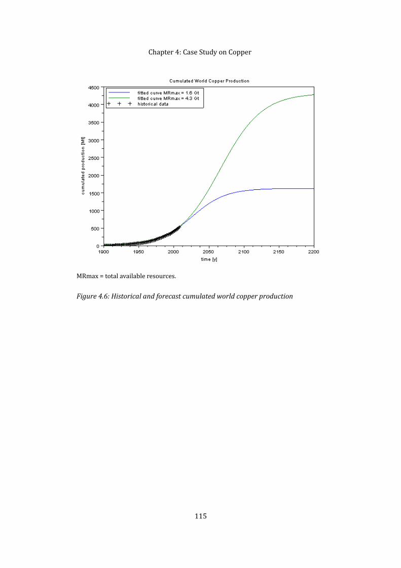
Chapter 4: Case Study on Copper

115

MRmax = total available resources.Figure 4.6: Historical and forecast cumulated world copper production

Chapter 4: Case Study on Copper

4.3.3 Geneva Share of Available Copper ResourcesAn attempt can now be made to try to determine the Geneva share of the world copper resources. The period of interest is here 2000–2080. Let us assume that the Geneva share of world production remains at the year 2000 level or at about 0.0116%. This value is obtained by dividing the primary copper consumption of the Canton of Geneva (imports minus product exports minus scrap exports) in 2000 (Faist Emmenegger & Frischknecht 2003) by the world mine production (USGS 2010a). In comparison, the Canton represented only about 0.0068% of the world’s population in 2000 (United Nations 2010; OCSTAT 2011c). The evolution of Geneva’s share of world copper production and resources can be seen in Figures 4.8 and 4.9.

116

MRmax = total available resources.Figure 4.7: Predicted available world copper resources

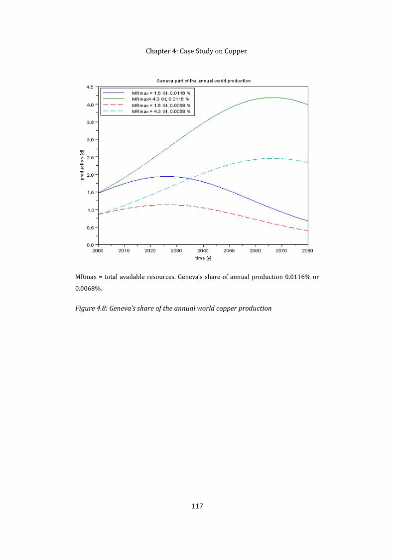
Chapter 4: Case Study on Copper

117

MRmax = total available resources. Geneva’s share of annual production 0.0116% or 0.0068%.Figure 4.8: Geneva’s share of the annual world copper production

Chapter 4: Case Study on Copper

4.4 AutarkyBased on scenarios regarding resource consumption and Geneva’s share of world resources (0.0116%), the annual primary copper consumption can now be compared with the annual production (Figure 4.10). In the case of available resources of 4.3 Gt, there is still no concern with regard to resource supply whereas in the case of 1.6 Gt of available resources, the part allocated to the Canton of Geneva becomes rapidly smaller than the resource needs. The consumption surpasses production first for the e-mobility scenario (close to the year 2030), then for the baseline and the building waste scenario (in the 2040s and the 2050s respectively). The substitution scenario follows in the somewhat more distant future (in the 2070s). The ‘No Primary Copper’ scenario is not studied here for two reasons: firstly, it represents a more theoretical alternative and not a plausible future. On the other hand, the resource needs in the Canton are completely satisfied by secondary copper in this scenario and 118

MRmax = total available resources. Geneva’s share of available resources 0.0116% or 0.0068%.Figure 4.9: Geneva’s share of available world copper resources

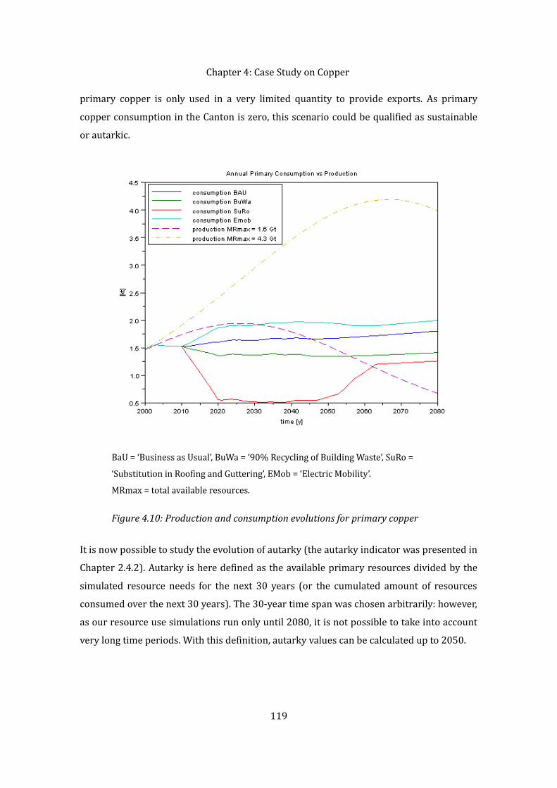
Chapter 4: Case Study on Copper primary copper is only used in a very limited quantity to provide exports. As primary copper consumption in the Canton is zero, this scenario could be qualified as sustainable or autarkic.

It is now possible to study the evolution of autarky (the autarky indicator was presented in Chapter 2.4.2). Autarky is here defined as the available primary resources divided by the simulated resource needs for the next 30 years (or the cumulated amount of resources consumed over the next 30 years). The 30-year time span was chosen arbitrarily: however, as our resource use simulations run only until 2080, it is not possible to take into account very long time periods. With this definition, autarky values can be calculated up to 2050.

119

BaU = ‘Business as Usual’, BuWa = ‘90% Recycling of Building Waste’, SuRo = ‘Substitution in Roofing and Guttering’, EMob = ‘Electric Mobility’.MRmax = total available resources. Figure 4.10: Production and consumption evolutions for primary copper

Chapter 4: Case Study on Copper Our definition of autarky is unorthodox in the sense that it is not based on the resources extracted in the Canton but the Canton’s share of global resources.

The autarky values for the different scenarios are shown in Figure 4.11. In the baseline scenario, autarky is less than 10 years during the entire simulation period. In the case of the first resource hypothesis (1.6 Gt of available resources), the autarky values descend from about 3 years to only one year in 2050. The electric mobility and recycling scenarios follow ‘Business as Usual’ fairly closely; in the second resource hypothesis (4.3 Gt of available resources), the autarky differences are at most about two years. In the first resource hypothesis, the difference in autarky values is at its greatest only half a year. In general, the electric mobility scenario is somewhat closer to the baseline scenario than the building waste scenario. The substitution scenario on the other hand has mostly much higher autarky values, with final autarky values of about 1.4 (1.6 Gt of available resources) and 9.6 years (4.3 Gt of available resources).

120

Chapter 4: Case Study on Copper

To extend the scope of the forecast, it is possible to define autarky using the current rather than predicted resource consumption: in this case, the predicted resource consumption over the next 30 years is replaced with the current annual consumption times 30 (see Chapter 2.4.2). The autarky values obtained in this manner are very similar to the earlier ones since the resource consumption grows in an almost linear manner and not for instance exponentially (Figure 4.12). However, the autarky curve based on current annual consumption is much less smooth than that based on the predicted consumption evolutions; this is because the annual primary copper consumption is more volatile. The annual primary resource consumption depends on for instance the amount of recycled copper which varies annually as a result of past population growth phenomena. 121

BaU = ‘Business as Usual’, BuWa = ‘90% Recycling of Building Waste’, SuRo = ‘Substitution in Roofing and Guttering’, EMob = ‘Electric Mobility’.MRmax = total available resources. Figure 4.11: Autarky based on simulated copper consumption

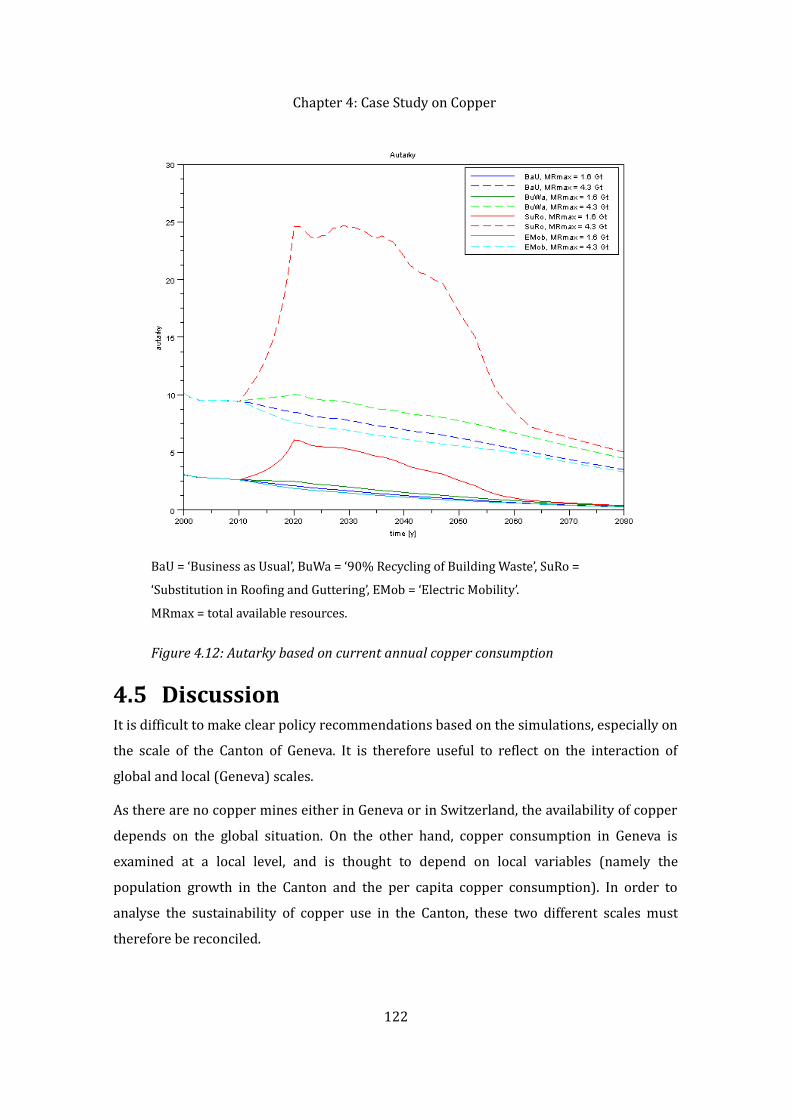
Chapter 4: Case Study on Copper

4.5 DiscussionIt is difficult to make clear policy recommendations based on the simulations, especially on the scale of the Canton of Geneva. It is therefore useful to reflect on the interaction of global and local (Geneva) scales. As there are no copper mines either in Geneva or in Switzerland, the availability of copper depends on the global situation. On the other hand, copper consumption in Geneva is examined at a local level, and is thought to depend on local variables (namely the population growth in the Canton and the per capita copper consumption). In order to analyse the sustainability of copper use in the Canton, these two different scales must therefore be reconciled. 122

BaU = ‘Business as Usual’, BuWa = ‘90% Recycling of Building Waste’, SuRo = ‘Substitution in Roofing and Guttering’, EMob = ‘Electric Mobility’.MRmax = total available resources. Figure 4.12: Autarky based on current annual copper consumption

Chapter 4: Case Study on Copper The global copper availability depends on the global copper production and demand over which the decision makers in the Canton have little or no influence. The global demand for refined copper has increased on average by 4% yearly since the beginning of the 20 th century (ICSG 2009). The copper demand is driven by Asian countries (especially China) where the demand doubled in a period of 15 years, from 1993 to 2008 (ICSG 2009). China has become the biggest refined copper user and if its recent economic growth continues, it will continue to drive the global copper demand. In view of the growth in China, it is likely that Swiss and Geneva shares of the global copper resources shall actually decrease in the coming decades. Based on a UN population projection, the world population is expected to continue to rise to just over 9 billion in 2050 (United Nations 2011); this would also mean that Geneva’s share of the world population will decline. Europe’s share of the world population is actually predicted to decline from 11% to less than 7% by 2100 (United Nations 2011). However, it is not sure whether the continent with the biggest population growth, Africa, shall command a greater portion of global resources. Clearly, the pressure on available resources shall continue to rise in the future. As the Canton of Geneva can hardly influence global developments, it should focus its actions on the aspects that are (at least to some degree) under its control: namely, copper demand, use, and recycling in the Canton. 4.6 ConclusionIn this chapter, a dynamic MFA model was constructed for copper metabolism in the Canton of Geneva; this model was then used to simulate the evolution of copper stocks and flows in the coming decades. In addition to a baseline scenario, four alternative resource use scenarios were formulated. One scenario examined the benefits of increased recycling of building waste, another focused on the substitution of copper in roofing and guttering, and a third scenario assessed the impacts of a transition to electric mobility. A fourth scenario was a purely theoretical illustration of a completely self-sufficient situation in terms of copper use: the Canton’s needs were assumed to be entirely covered by recycled copper. In addition, a Hubbert’s peak model was constructed to illustrate the future availability of global copper resources.

123

Chapter 4: Case Study on Copper The substitution and recycling scenarios allowed the reduction of primary copper consumption by about 20–30% by 2080. These reductions are not insignificant but they have no influence on the overall trend of copper consumption, which increases following population growth. In addition, since the copper recycling rate is already high (about 80%), it would probably be technically and economically difficult to increase it significantly. As regards substitution, although substitutes such as aluminium may be less scarce than copper, the environmental impacts of their extraction and production might be such that these resources can scarcely be said to constitute a preferable alternative. Increasing resource use efficiency remains an alternative, although difficult to put into practice at a cantonal level as copper extraction and refining takes place outside the Canton. In the e-mobility scenario, copper use increases slightly (net imports increase by 6% compared to the baseline scenario) whereas the ‘No Primary Copper’ scenario would require quite drastic changes in the Canton’s copper consumption: in this scenario, net imports decrease by more than 60% by 2080. Indeed, it is only when copper consumption has reached a stable level or declines, that recycling can provide a means to satisfy a significant percentage of copper needs and become in an effective manner ‘a part of the solution’ (Grosse 2010). The sensitivity analysis reveals, unsurprisingly, that the model results are highly sensitive to the copper consumption per capita parameter. In order to significantly reduce the Canton’s copper use, efforts should be made to decrease the per capita consumption. However, this might not be sufficient to lead to an absolute dematerialization as the reduction in the per capita consumption can be cancelled out by population growth. In terms of future developments in the dynamic MFA model, it would, for instance, be possible to use a residence time distribution for copper products instead of a fixed residence time (for more information see Chapter 3.2.2). It could also be possible to model the transitions in different scenarios as logistic curves instead of linear changes. Undoubtedly, it would be worthwhile collecting more up-to-date and accurate data on the copper stocks and flows as well as defining data uncertainties: the predictions of our dynamic MFA model can only be as good as the underlying data.

124

Chapter 5: Case Study on PhosphorusChapter 5 Case Study on PhosphorusThis case study begins with an introduction to the uses and importance of phosphorus and a description of the issue of peak phosphorus (Chapter 5.1). The phosphorus metabolism is examined closer in Switzerland (Chapter 5.2) and in the Canton of Geneva (Chapter 5.3). Later, a dynamic phosphorus metabolism model is constructed and the evolution of phosphorus use in the Canton of Geneva is simulated (Chapter 5.4). An uncertainty analysis of the model results is also included (Chapter 5.5). The study ends with a discussion and a conclusion (Chapter 5.6). 5.1 Introduction5.1.1 On the Importance of PhosphorusPhosphorus is an element that is essential for all living organisms: no life is possible without it (Smil 2000; Liu et al. 2008). As one of the three vital crop nutrients—along with nitrogen and potassium—phosphorus is crucial to plant growth and thus to the entire agricultural system. Although phosphorus is a relatively common element on Earth (11th in the lithosphere), it is not without its scarcity issues (EFMA 2000; Smil 2000). Phosphorus is frequently a limiting growth factor owing to two reasons: firstly, it is rather scarce in the Biosphere and, secondly, only a small proportion of the phosphorus present in soil is available for plant use (Smil 2000; Liu et al. 2008). These reasons could be qualified as quantitative and qualitative scarcity. The transformations of phosphorus compounds and soil chemistry are not presented here in further detail (for more information see, for example, EFMA 2000; Frossard et al. 2004; Liu et al. 2008). Around 90% of the global phosphorus demand is related to food production in the form of fertilizers, animal feed, and feed additives (Cordell et al. 2009). Other phosphorus uses include for instance detergents—these products represent approximately 7% of the phosphorus demand in Western Europe—and various speciality uses such as corrosion inhibitors, flame retardants, water treatment and ceramic production (remaining 3%) (EFMA 2000; Smil 2000). A secure phosphorus supply is therefore essential to global food security, which FAO (2010) defines as follows:Food security exists when all people, at all times, have physical and economic access to sufficient, safe and nutritious food for a healthy and active life ....

125

Chapter 5: Case Study on PhosphorusThis involves 4 conditions:1. adequacy of food supply or availability2. stability of supply, without fluctuations or shortages from season to season or from year to year3. accessibility to food or affordability4. quality and safety of foodA sufficient phosphorus supply is vital to food security.

Phosphorus has been historically obtained from diverse sources such as farmyard manure, various organic wastes (bones, ash, and fish), night soil, and guano (Cordell et al. 2009). However, with the intensification of food production and the rise of cities, mineral fertilizers began to be employed more and more frequently (Liu et al. 2008). The Green Revolution further increased mineral fertilizer use. Mineral fertilizers are produced using mined phosphate rock; phosphate rock is first converted to phosphoric acid which is then further used to make fertilizers (Liu et al. 2008). One kilogram of phosphorus corresponds to approximately 2.29 kg of phosphate fertilizer P2O5 (EFMA 2000). The increased fertilizer use has also brought on the phenomenon of eutrophication which has since the 1950s been considered as the most significant environmental problem caused by phosphorus losses (Liu et al. 2008). A large amount of phosphorus is lost in the processes of erosion and run-off; the quantity has even been estimated to amount to one half of the phosphorus extracted yearly (Liu et al. 2008). Human activities have intensified phosphorus cycles and broken the historical recycling loop that existed in traditional agricultural systems (Liu et al. 2008). However, the soil-crop-animal-human-soil cycle of phosphorus could be closed anew by increasing the recycling of human and animal wastes. For instance, introducing urine-diverting toilets such as the NoMix toilets of Eawag would permit the use of urine as a liquid fertilizer or recover the required nutrient to be used in a solid form (Eawag 2007). In addition to phosphorus, nitrogen can also be recovered from urine and used as a fertilizer (Karak & Bhattacharyya 2011). Several field experiences have already been conducted and the solution appears feasible (University of Hohenheim et al. 2009; Karak & Bhattacharyya 2011); it has also been shown that the phosphorus present in urine is at least as available 126

Chapter 5: Case Study on Phosphorusto plants as the phosphorus in soluble fertilizers (Kirchmann & Pettersson 1995). In addition, the acceptability of this solution is surprisingly high: in one study, 42% of interviewed Swiss farmers stated they were willing to buy a urine-based fertilizer and 57% stated they thought urine recycling to be a good or very good idea (Lienert et al. 2003). However, cross-contamination and the potential presence of micro-pollutants remain a problem (Karak & Bhattacharyya 2011). Other possibilities include more intense recycling of sewage sludge and animal manure although these options also have their downsides: the presence of heavy metal contaminants in the sludge can make recycling problematic and the transportation costs and collection difficulties limit the use of manure (EFMA 2000). Besides increased recycling, options to decrease phosphorus consumption include reduced fertilizer application, prevention of losses from agricultural systems, reduction of livestock production, and limitation of losses in various phosphorus-related production processes (Vuuren et al. 2010). Phosphorus capture from water using algae has also been studied by the US Department of Agriculture (Perry 2010) but it remains under development. Phosphorus recovery from fly ash is also being examined (Slibverwerking Noord-Brabant 2011). 5.1.2 Peak PhosphorusThe four biggest phosphate rock producing countries are currently China, the United States, Morocco (Western Sahara), and Russia (USGS 2010b). In 2010, the total world reserves of phosphate rock were estimated at 16 Gt which corresponds approximately to a 100 years’ lifetime at the production rate of 2008 or 161 Mt (USGS 2010b). The countries with the biggest phosphate rock reserves were thought to be Morocco (Western Sahara), China, Jordan, South Africa, and the United States with 36%, 23%, 9%, 9%, and 7% respectively of the world reserves (USGS 2010b). However, the USGS has recently reviewed its estimates and the Moroccan reserves have risen from 5,7 Gt to 50 Gt thus increasing the world reserves to a total of 65 Gt and the static lifetime to nearly 400 years (USGS 2011). According to this recent information, Morocco effectively controls nearly 80% of the global phosphate rock reserves while the four biggest producer countries produce over 70% of all phosphate rock (USGS 2011). For the basis of comparison, 12 OPEC countries control nearly 80% of proven oil reserves and the four biggest producing countries produce less than 40% of the world production (BP 2010). Although the United States is currently one

127

Chapter 5: Case Study on Phosphorusof the major phosphate producers, it also imports phosphorus for its own consumption as the domestic production levels are insufficient and have already peaked (Déry & Anderson 2007; USGS 2010b). Phosphorus demand is expected to continue growing in the future: for instance, FAO has estimated that the annual growth rate for phosphate fertilizers will be 2.0% in 2011 and 2012, and a longer time-scale baseline scenario assumes an annual growth rate of 1.1% (FAO 2008a; FAO 2000). Recent estimates by the International Fertilizer Industry Association predict growth rates as high as 3% beyond 2011 (Heffer & Prud’homme 2010). The historical fertilizer consumption growth rate was around 2.1% during the past decade (Heffer & Prud’homme 2010). An annual demand growth rate of 1–3% would reduce the world reserves’ lifetime to 50–70 years. As phosphorus is mainly obtained from phosphate rock, the peaking of phosphate rock is likely to lead to a peak in phosphorus. The peak in phosphorus production was recently estimated to take place in the 2030s (Cordell et al. 2009; Cordell 2010). In fact, global phosphate rock production already experienced a minor peak in 1988, as seen in Figure5.1. Most sources explain this peak by a decrease in phosphate fertilizer demand in Europe and in the United States due to the maturing of the markets (Bumb & Baanante 1996; FAO 2000; Cordell et al. 2009), although the recessions of the 1980s and the early 1990s might also have had an influence (Sullivan et al. 2000) as well as the collapse of the Soviet Union, formerly a major consumer (Cordell et al. 2009). Indeed, it is interesting to note that the current economic crisis has also affected fertilizer demand similarly to the fate of other commodities such as copper (FAO 2008b). However, there has been some speculations on the idea that the peak close to 1990 was the true peak of ‘easy phosphate’ (Déry & Anderson 2007; Ward 2008). On the other hand, some authors estimate that there is no immediate cause for concern although the situation is worrying in the long run (Vuuren et al. 2010). Others estimate that there is no peak in sight while the closing of the phosphorus cycle is necessary for environmental reasons, notably for eutrophication (Scholz 2011). It should, however, be noted that the crucial time point is not that which corresponds to the total depletion of a resource: the problems begin when the maximum production rate is reached and the supply can no longer feed the growing demand (Diederen 2010, p. 49).

128

Chapter 5: Case Study on Phosphorus

Other problems related to the phosphate rock supply include declining ore grades which are related to the cost of phosphate recovery: an industry assessment indicates that the phosphate content of pre-beneficiated ore is already decreasing by around 1% per decade (Steen 1998). The International Fertilizer Industry Association estimates that the present reserves are only sufficient for 80 years at the present rate of production and with similar production costs whereas the reserves could last for 200 years at a somewhat higher cost (Isherwood 2000). Another problem is the energy costs: the energy required to produce mineral phosphate fertilizers is greater than that required by organic phosphate fertilizers (Cordell et al. 2009). During a single 14-month period in 2007–2008, rock phosphate prices increased by 700% and although the prices have since decreased, cheap fertilizers could soon be history (Cordell et al. 2009; Cordell 2011). For instance, changing diets in developing countries (increased consumption of meat and dairy products) and the expansion of biofuels could be responsible for the rise of prices (Cordell et al. 2009). China also recently imposed a 135% export tariff on phosphate in order to secure its domestic supply and radically diminish exports (Rosemarin et al. 2009). 129

Source: IFA (2010). Figure 5.1: World phosphate production from 1961 to 2008

Chapter 5: Case Study on PhosphorusAs phosphorus is a basic chemical element, it cannot be substituted in agriculture; but unlike some other non-renewable resources―such as oil―phosphorus can be recycled (Steen 1998; USGS 2010b). These two aspects (non-substitutability and recyclability) constitute the main difficulty and the main hope for future phosphorus management. There are no substitutes for phosphorus in food production.

5.2 Phosphorus Metabolism in SwitzerlandIn recent years, there have been several studies on phosphorus flows for instance in China (Chen et al. 2008), Japan (Matsubae-Yokoyama et al. 2009), Sweden (Schmid Neset et al. 2008), and Finland (Antikainen et al. 2005; Antikainen 2007) as well as in Switzerland (FOEN 2009b). The Swiss study is a comprehensive assessment of the phosphorus stocks and flows in Switzerland for the year 2006, its goal being to find ways to optimize resource management. In practice, the study employs the method of substance flow analysis. The mains system (Switzerland) is divided into six subsystems: Agriculture Animals, Agriculture Plants (including forestry, and pulp and paper industry), Chemical Industry, Households & Trade, Waste Sector, and Ground and Surface Waters. The data uncertainty was estimated to be smaller than 20% for over 80% of the flows. The results of the study are summarized in Figure 5.2.

130

Chapter 5: Case Study on Phosphorus

131Imp. = imports, exp. = exports.Source: FOEN (2009).Figure 5.2: Phosphorus metabolism in Switzerland in 2006

Chapter 5: Case Study on PhosphorusAll the following information stems from the Swiss SFA study (FOEN 2009b), unless indicated otherwise. There are no phosphate mines in Switzerland and the country is a net importer of phosphorus. The annual phosphorus imports amount to approximately 16,500 tP whereas exports constitute 3,900 tP. The phosphorus net imports per capita are therefore approximately 1.7 kg given that the Swiss population was about 7.6 million in 2006 (FSO 2011e). The imports consist mainly of animal feed and mineral fertilizers (imports by sectors are seen in Figure 5.3 and detailed imports in Figure 5.4) whereas the exports are comprised of surface and ground water flows, and offal and butcher waste from the food industry (exports by sectors are seen in Figure 5.5 and detailed exports in Figure 5.6).The phosphorus cycle is dominated by agricultural activities and waste disposal and, to a lesser extent, by households and trade. In the agricultural sector, an almost closed cycle exists, formed by the exchange of farmyard manure and animal feed (each containing nearly 30,000 tP) between the plant and animal production subsystems. However, the imports of animal feed and mineral fertilizers (5,600 tP and 5,900 tP) also play an important role. The greatest net addition to stock takes place in the waste sector (9,000 tP/year) and in the Agriculture Plants subsystem (3,500 tP/year). Phosphorus stocks in the soil therefore increase year after year. Other studies have also shown that past agricultural practices have resulted in phosphorus accumulation in the soil (Frossard et al. 2004). The most important sink in the waste sector are landfills (6,300 tP/year) followed by cement factories (2,800 tP/year). The waste sector handles about 13,500 tP annually; however, merely 12% of this phosphorus is recycled in agriculture or in private gardens. Annual phosphorus losses (as outflow from waste water treatment and as stocks in landfills and cement factories) are thus greater than 10,000 tP or nearly 90% of net phosphorus imports.

132

Chapter 5: Case Study on Phosphorus

133

The quantity of phosphorus in Households & Trade is so small that the percentage is rounded to zero. Source: FOEN (2009).Figure 5.3: Proportions of Swiss phosphorus imports to different subsystems

The quantity of phosphorus in animal imports and rainfall are so small that the percentages are rounded to zero. Source: FOEN (2009).Figure 5.4: Proportions of Swiss phosphorus imports

Chapter 5: Case Study on Phosphorus

134

Source: FOEN (2009).Figure 5.6: Proportions of Swiss phosphorus exports

Source: FOEN (2009).Figure 5.5: Proportions of Swiss phosphorus exports from different subsystems

Chapter 5: Case Study on Phosphorus5.2.1 Recycling ScenariosThe Swiss study concludes that phosphorus management is not yet organised optimally and that improvements could be made (FOEN 2009b). The study proposes four scenarios that attempt to better close the Swiss phosphorus cycle (FOEN 2009b):1. use of sewage sludge ahs as fertilizer2. use of meat and bone meal as fertilizer3. use of meat and bone meal as animal feed4. consequential recycling of green wasteThe Swiss study examines two variants of each scenario (except for the third one): one variant assumes 100% efficiency (optimal recycling) whereas the other―a more realistic one―takes into account various efficiency limitations (FOEN 2009b). The focus is here on the less efficient scenarios that provide a more realistic view of the recycling potential in the medium term. The following data on the scenarios stem from the Swiss Federal Office for the Environment study (FOEN 2009b). The first recycling scenario describes a situation where sewage sludge (containing about 7,500 tP/year in Switzerland) would be used as a fertilizer in agriculture. The use of sewage sludge as fertilizer was forbidden in 2003 due to health concerns as the sludge contains heavy metals. This heavy metal contamination is the main obstacle to the exploitation of the phosphorus-rich sludge. The scenario assumes that all Swiss sewage sludge is exploited in the form of sewage sludge ash; however, it is estimated that the efficiency of this fertilizer would only be 40% of that of mineral fertilizers.The second and third recycling scenarios explore the use of meat and bone meal (corresponding to approximately 3,000 tP yearly at Swiss level). Only a fraction of this quantity is currently exploited as pig feed whereas the rest is incinerated (50%) or exported abroad (50%). The second scenario assumes that meat and bone meal would be used as a fertilizer with 40% efficiency compared to mineral fertilizers. The third scenario assumes that meat and bone meal would be used as animal feed; meat and bone meal was largely replaced with imported soy after the BSE crisis. The fourth scenario deals with increased recycling of household green waste in anaerobic digestion and composting. At the moment, 880 kt of green waste is collected separately in Switzerland whereas 720 kt is incinerated with municipal waste (this gives a recycling rate 135

Chapter 5: Case Study on Phosphorusof 55%). In the Canton of Geneva, about 45% of organic waste is incinerated with municipal waste (Faessler et al. 2010). The FOEN scenario assumes that about 60% of this non-exploited green waste (or 450 kt) could be recycled. When taking into account efficiency and feasibility factors, the first and second recycling scenarios (the use of sewage sludge or meat and bone meal as fertilizer) would allow the reduction of mineral fertilizer imports by approximately 20%. Green waste recycling would have a lesser effect: it would only allow a reduction of about 7%. The use of meat and bone meal as animal feed could reduce animal feed imports by 50%. Combining three different recycling possibilities (scenarios 1, 2, and 4) would allow almost a 50% reduction in mineral fertilizer imports but, on the other hand, phosphorus accumulation in agricultural soils would more than double. Overall, the greatest potential for optimisation of the phosphorus cycle seems to lie in the management of sewage sludge along with the recycling of offal and butcher waste. The potential of green waste is lower since this resource is already moderately well exploited. 5.3 Phosphorus Metabolism in the Canton of Geneva5.3.1 Normalizing the Swiss Metabolism StudyThere is very little conclusive information on the phosphorus flows in the Canton of Geneva. Some information can be obtained indirectly via the material flow analyses of wood and various agricultural products (see, for example, Faist Emmenegger & Frischknecht 2003; Faessler et al. 2010). It is for this reason that I decided to use the detailed Swiss metabolism study as the main source of information. Naturally, the study needed to be normalized from federal level to the Canton of Geneva and adapted to the Canton’s characteristics. The subsystems of the Swiss study were individually scaled to the Geneva scale. The normalization was done based on several different Geneva/Switzerland ratios shown in Table 5.1.The normalization ratios are defined as follows:

– The population ratio POPU is applied to the household sector (except for the quantity of rainfall).136

Chapter 5: Case Study on Phosphorus– The agricultural production ratio AGAN is applied to the ‘Agriculture Animals’ subsystem.– The agricultural production ratio ANPL is applied to the ‘Agriculture Plants’ subsystem (with the exception of the forest sector).– The chemical exports ratio CHIN is applied to the chemical industry.– The wood products ratio WOPR is applied to wood products produced in the Canton (a part of the forest sector).– The wood energy ratio WOEN is applied to the wood energy production in the Canton (a part of the forest sector).– The paper ratio PAPE is applied to paper production in the Canton (a part of the forest sector).– The rainfall ratio RAIN ratio is applied to the quantity of rainfall.Various interactions must also be taken into account in the normalization, for instance an increased amount of compost and digestate diminishes the amount of mineral fertilizer imports, and a decreased paper production leads to more paper imports.The results of the normalization can be seen in detail in Appendix C and they are also summarized in Figure 5.7.According to the results of the normalization, the phosphorus imports in the Canton of Geneva represent about 1,400 tP/year and the exports amount to nearly 900 tP/year. The sectorial imports and exports can be seen in Figures 5.8 and 5.9 and the product details in Figures 5.10 and 5.11. Net imports per capita are approximately 1.1 kg or about 30% less less than those on a national level (1.7 kg per capita). This results from the lesser importance of the agricultural sector since only direct phosphorus imports are taken into account. The majority of phosphorus imports are destined for agriculture, mainly in the form of mineral fertilizers (67%). In addition, food imports represent an important part of the imported phosphorus (29%). Animal feed exported from the agricultural sector represents nearly 90% of exports whereas the flow of ground and surface waters accounts for 10%. The main difference with the Swiss phosphorus metabolism is the fact that food imports are much more important in Geneva as the portion of agriculture is smaller. Mineral fertilizer imports and animal feed exports also represent a greater share

137

Chapter 5: Case Study on Phosphoruscompared to those on a federal level as the importance of animal agriculture is much smaller.The yearly addition to stock amounts to 500 tP, waste sector (landfills and cement factories) accounting for 80% and agriculture (soils) for 20%. About 16% of the phosphorus treated annually in the waste sector is recycled in gardening or agriculture whereas about 80% of it is lost in outflow, landfills, and cement factories.

138

Chapter 5: Case Study on PhosphorusTable 5.1: Geneva/Switzerland normalization ratios

Population (POPU)

Agriculture Plants (AGPL)

Agriculture Animals (AGAN)

Chemical Industry (CHIN)

Wood Products (WOPR)

Wood Energy (WOEN)

Paper (PAPE) Rainfall (RAIN)

Indicator [unit] Mean resident population Food of plant origin [t] Food of animal origin [t] Chemical industry exports [1,000 CHF] Wood products [t] Wood energy [t] Paper [t] Rainfall [mm] x Surface area [km2]Value GE 439,785 60,063 3,489 2,122,615 540 4,860 0 954 x 282.2 Value CH 7,557,609 2,190,000 3,926,000 62,974,872 1,415,774 3,150,595 1,657,000 1,272 x 41,284.8Ratio GE/CH 5.82% 2.74% 0.09% 3.40% 0.04% 0.15% 0.00% 0.51% Source GE FSO (2010d) Faessler et al. (2010) Faessler et al. (2010) OCSTAT (2010) Faessler et al. (2010) Faessler et al. (2010) Faist Emmenegger & Frischknecht (2003) MeteoSwiss (2010), FSO (2010e)Source CH FSO (2010d) FOEN (2009b) FOEN (2009b) OCSTAT (2010) FOEN (2009b) FOEN (2009b) FOEN (2009b) MeteoSwiss (2010), FSO (2010e)Reference year GE 2006 2009 2009 2006 2009 2009 2000 1961-1990 (precipitations), 2006 (area)Reference year CH 2006 2006 2006 2006 2006 2006 2006 1961-1990 (precipitations), 2006 (area)GE = Geneva, CH = Switzerland. Precipitations in Geneva: Geneva-Cointrin station; precipitations in Switzerland: Swiss average (all stations). Source: (Faist Emmenegger & Frischknecht 2003; FOEN 2009b; Faessler et al. 2010; FSO 2011e; FSO 2011f; MeteoSwiss 2010; OCSTAT 2011b)

139

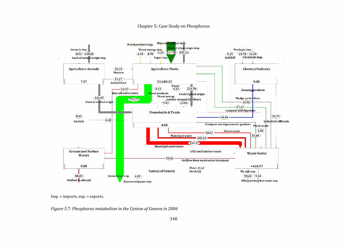
Chapter 5: Case Study on Phosphorus

140Imp. = imports, exp. = exports.Figure 5.7: Phosphorus metabolism in the Canton of Geneva in 2006

Chapter 5: Case Study on PhosphorusIn reality, the total amount of phosphorus needed to provide for the needs of the Geneva population is much higher: our study only accounts for the direct phosphorus flows whereas the phosphorus quantity in indirect flows could be much higher. For instance, in optimal settings 90% of phosphorus incorporated in fertilizers can be exploited by plants (Syers et al. 2008). Therefore, one kilogram of phosphorus in crops necessitates at least 1.1 kg of phosphorus as fertilizer. 1 kgP in meat requires 4.6 kgP in grain and thus more than 5 kg of phosphorus fertilizer, assuming that it takes 7 kg of animal feed to produce 1 kg of meat4 and that the phosphorus concentrations are 3.09 and 4.75 gP/kg respectively (FOEN 2009b). This calculation increases the quantity of phosphorus flows related to imports from 1,400 tP to 2,200 tP or an increase of 60%. The real phosphorus use ought to be even higher due to losses in agriculture, fertilizer manufacturing, and phosphate mining.

According to the Swiss metabolism study, the stocks in ‘Households & Trade’ and ‘Ground and Surface Waters’ processes are zero whereas the waste sector stocks are unknown. This leaves us with an agricultural sector whose stocks have been estimated at approximately 9 4 Actually, it takes 12 kg of grain to obtain 1 kg of beef, 5 kg of grain to obtain 1 kg of pork, 16 kg of grain for 1 kg of sheep, and only 2 kg of grain for 1 kg of chicken (USDA 2009). 7 kg has been used as a conservative approximation. 141

The quantity of phosphorus in Households & Trade is so small that the percentage is rounded to zero.Figure 5.8: Proportions of Geneva’s phosphorus imports to different subsystems

Chapter 5: Case Study on PhosphorusMt. Normalized to the Geneva scale with the AGAN and ANPL ratios, the stock values of about 7.37 t and 22,700 t are obtained for animal and plant agriculture.

142

The quantity of phosphorus in animal imports and rainfall are so small that the percentages are rounded to zero.Figure 5.9: Proportions of Geneva’s phosphorus imports

Figure 5.10: Proportions of Geneva’s phosphorus exports from different subsystems

Chapter 5: Case Study on Phosphorus

5.3.2 Confrontation of DataSeveral alternative ratios could have been used to normalize the Swiss SFA study; for instance, instead of looking at the quantity of food production of animal and plant origin, it would have been possible to compare the agricultural land areas (grazing area excluded) and the numbers of livestock in Geneva and Switzerland. This would have given us respectively 2.89% (reference year 2007) and 0.25% (reference year 2009) (FSO 2011c; Swiss Farmers’ Union 2011). As regards the chemical industry, information was not available on the production quantities and therefore the values of chemical product exports have been compared. It would also have been possible to compare the number of employees in this domain, which would have given a very different result—9.28% Geneva/Switzerland ratio in 2008 (FSO 2011a; OCSTAT 2005a). However, as coking and refining industries were also included in the same federal statistics category, it was decided that the value of exports might be a more accurate indicator. Additional information on the quantity of wood products and energy is also available. According to the Swiss Federal Statistical Office, the proportion of wood products and wood energy production in Geneva in the year 2006 would have been 0.04% and 0.15% respectively (FSO 2011d). It is not quite clear why this statistic does not correspond entirely to the information provided by Faessler et al. (2010) and FOEN (2009b). However, 143

The quantity of phosphorus in offal and butcher waste is so small that the percentage is rounded to zero.Figure 5.11: Proportions of Geneva’s phosphorus exports

Chapter 5: Case Study on Phosphorusit is somewhat difficult to compare the different data as they do not use the same unit (m 3 and tonnes) and only Faessler et al. (2010) clearly denote their assumptions on timber humidity. The relation of m3 and tonnes depends notably on the wood essence and its humidity. The data from Faessler et al. (2010) and correspondingly FOEN (2009b) on a Swiss federal level, were chosen in order to keep the results in accord with the wood metabolism study which also exploits the same data.It is also interesting to note that the data from the year 2000 metabolism study in Geneva (Faist Emmenegger & Frischknecht 2003) do not quite match the data from the more recent metabolism study (Faessler et al. 2010). According to the first study, the amount of wood mobilised in the Canton corresponds to approximately 4.2 kt whereas the more recent study arrives at 5.4 kt. However, this difference could be explained by an increase in the exploitation rate. A greater problem is the fact that the wood consumption given by the year 2000 study (41.7 kt in total) is not of the same order of magnitude as the value obtained by normalizing the Swiss study based on the population size (about 220 kt). In addition, the share of wood energy in the total wood consumption is quite different: 12% (Faist Emmenegger & Frischknecht 2003) versus 69% (FOEN 2009b). The data for paper consumption are more in accord: the year 2000 study arrives at 95.5 kt (paper and cardboard) whereas normalizing the Swiss study gives us 104 kt.5.3.3 Recycling ScenariosThe original Swiss metabolism study explored five scenarios and four of these scenarios (‘Business as Usual’, ‘Sewage Sludge as Fertilizer’, ‘Meat and Bone Meal as Fertilizer’, and ‘Recycling of Green Waste’) were also explored in the Canton of Geneva. The scenario ‘Meat and Bone Meal as Animal Feed’ was left out since it was redundant next to ‘Meat and Bone Meal as Fertilizer’ (in terms of the reused material) and it also posed complex health considerations. The three recycling scenarios were normalized in the same manner as the baseline scenario (see Appendix C for details). The influences of these scenarios at the Geneva level are presented here briefly. The sewage sludge scenario allows the reduction of mineral fertilizer inputs by 12% whereas the meat and bone meal (MBM) and green waste recycling scenarios only allow reductions of 0.1% and 3% respectively. Total imports are reduced by 8% (sewage sludge scenario) and 2% (green waste recycling scenario).

144

Chapter 5: Case Study on PhosphorusThe yearly addition to stock in agriculture (plants) increases in both the sewage sludge and meat and bone meal scenarios (+130% and +2%) whereas the green waste scenario does not prompt any change. Net addition to landfills decreases in the sewage sludge and green waste recycling scenarios (-59% and -7%) whereas the outflow to water systems remains identical. In the MBM scenario, the addition to landfills and water systems remains practically identical to the ‘Business as Usual’ scenario. With regard to the waste sector, in the sewage sludge scenario 58% of the inputs are recycled as opposed to 21% in the green waste scenario. The recycling rate of MBM remains identical to the ‘Business as Usual’ scenario (16%).All in all, the meat and bone meal and green waste recycling scenarios resemble the ‘Business as Usual’ scenario quite closely whereas the sewage sludge scenario creates more changes in the system. It is not very surprising that the recycling of meat and bone meal in Geneva does not allow a significant reduction in phosphate fertilizer imports since the weight of livestock is fairly small. On the other hand, green waste recycling achieves better results as the Canton is densely populated compared to the Swiss average. This is also the reason why sewage sludge could become an important phosphorus source in the future. In addition to the FOEN scenarios, the possible use of human urine as fertilizer has been inspected. The impacts of human urine recycling can be briefly calculated as follows. The Geneva population in 2010 was about 460,000, each person producing as much as 0.5 kgP in urine per year (University of Hohenheim et al. 2009); some sources cite figures as high as 0.7–1.0 kgP/person/year (Karak & Bhattacharyya 2011). This means that a total of 220–450 t of phosphorus becomes available yearly through human urine. About 920 t of phosphorus in mineral fertilizers are imported yearly in the Canton of Geneva (Chapter 5.3.1); complete human urine recycling could thus permit a reduction of about 25–50% in fertilizer imports. Let us assume that 0.5 kgP/year could be recovered for each inhabitant of Geneva, corresponding to a total of about 220 tP. In this scenario, the phosphorus mineral fertilizer imports would be reduced by 22% and the overall imports by 8%. The recycling rate would increase to 51% while the phosphorus stocks in the waste sector would decrease by 40%. For more information on the urine recycling scenario, see Appendix C.145

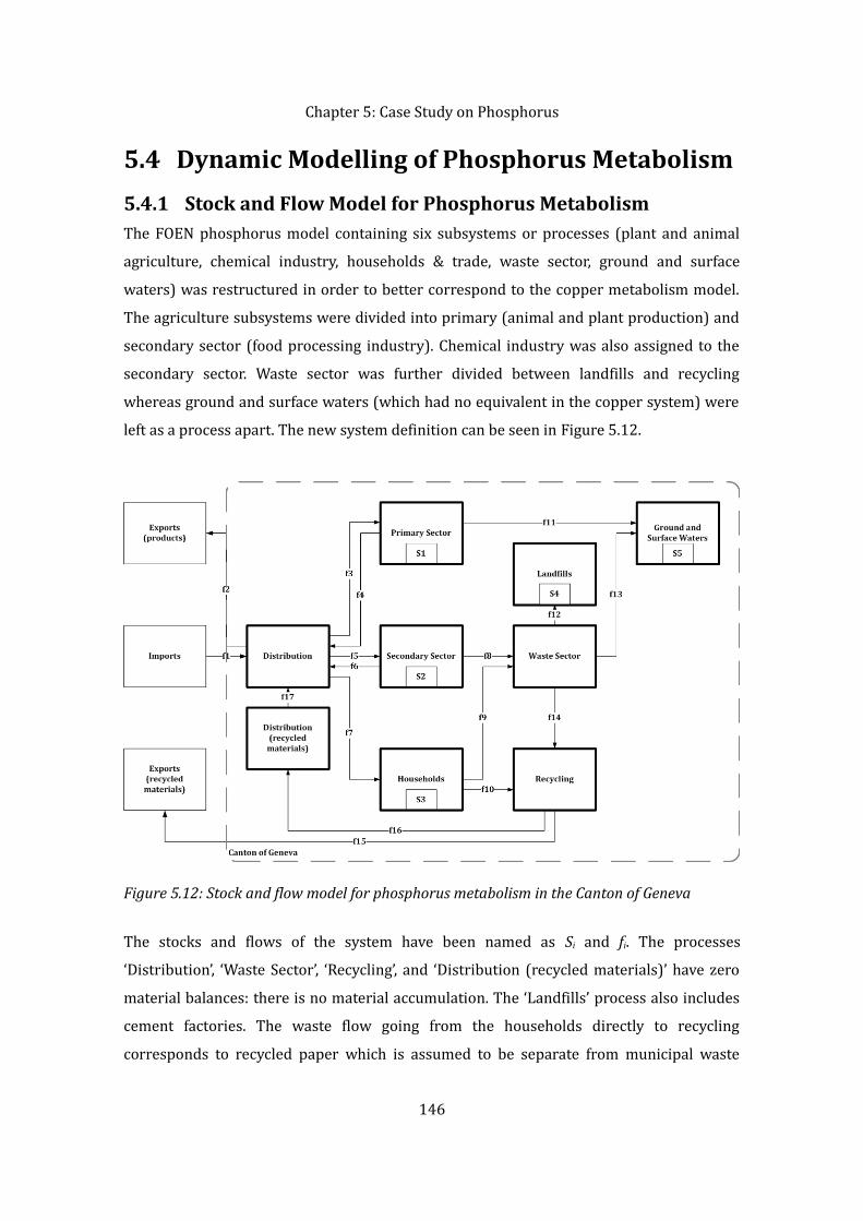
Chapter 5: Case Study on Phosphorus5.4 Dynamic Modelling of Phosphorus Metabolism5.4.1 Stock and Flow Model for Phosphorus MetabolismThe FOEN phosphorus model containing six subsystems or processes (plant and animal agriculture, chemical industry, households & trade, waste sector, ground and surface waters) was restructured in order to better correspond to the copper metabolism model. The agriculture subsystems were divided into primary (animal and plant production) and secondary sector (food processing industry). Chemical industry was also assigned to the secondary sector. Waste sector was further divided between landfills and recycling whereas ground and surface waters (which had no equivalent in the copper system) were left as a process apart. The new system definition can be seen in Figure 5.12.

The stocks and flows of the system have been named as Si and fi. The processes ‘Distribution’, ‘Waste Sector’, ‘Recycling’, and ‘Distribution (recycled materials)’ have zero material balances: there is no material accumulation. The ‘Landfills’ process also includes cement factories. The waste flow going from the households directly to recycling corresponds to recycled paper which is assumed to be separate from municipal waste 146

Figure 5.12: Stock and flow model for phosphorus metabolism in the Canton of Geneva

Chapter 5: Case Study on Phosphorusdestined for the waste sector for further sorting and treatment. The subsystem ‘Ground and Surface Waters’ has been drawn inside the system borders although in reality the phosphorus flows in water systems can also end up outside the Canton’s borders. The processes (subsystems) are detailed in Table 5.2.Table 5.2: Phosphorus system processes

Process Name Process Description Change in StockImports Imports of phosphorus containing goods from outside the Canton -

Exports (products) Exports of phosphorus containing goods -Distribution Distribution of phosphorus containing goods (imports, exports, and recycled phosphorus) to the economic sectors NoPrimary Sector Use of phosphorus in the primary sector (agriculture, forestry) Yes

Secondary Sector Use of phosphorus in the secondary sector (food processing and chemical industry) YesHouseholds Use of phosphorus in households YesWaste Sector Treatment of phosphorus containing waste NoLandfills Landfilling of phosphorus-containing waste from incineration & the use of phosphorus-containing waste in cement factories Yes

Ground and Surface Waters Dispersion of phosphorus in ground and surface waters in and outside of the Canton (via erosion and waste water) YesRecycling Collection and recycling of phosphorus containing waste NoDistribution (recycled materials) Distribution of phosphorus containing recycled goods to the economic sectors No

Exports (recycled materials) Exports of phosphorus containing waste to be recycled outside the Canton -This stock and flow model has in total 27 unknowns:

147

Chapter 5: Case Study on Phosphorus– 17 flows– 5 stocks – 5 changes in stock27 equations are therefore needed to solve the system (see Appendix C for details).

5.4.2 Precision on VocabularySome precisions on the vocabulary used: – The total phosphorus consumption in the Canton corresponds to flows f1 + f17.

– Apparent consumption corresponds to f1 – f2 + f17.

– The amount of net imports corresponds to f1 – f2.

– Primary phosphorus consumption corresponds to net imports – exports of recycled materials, f1 – f2 – f15.

– The amount of phosphorus recycled in the Canton corresponds to the flow f17.

5.4.3 Phosphorus Metabolism ScenariosThe different possibilities for the evolution of the system are presented in the form of chosen scenarios. The examined scenarios include:– Business as Usual– Sewage Sludge as Fertilizer– Meat and Bone Meal as Fertilizer– Recycling of Green WasteThe characteristics of the scenarios studied are summarized in Table 5.3.The ‘Business as Usual’ scenario is seen as a continuation of the current tendencies whereas the other three scenarios reflect increased recycling as defined in the FOEN (2009b) study. In practice, all four scenarios share the same basic assumptions about system behaviour, only the values of parameters characterizing this behaviour are adjusted. These parameters are based on the initial stock and flow values obtained from the normalized metabolism scenarios (see Chapter 5.3).

148

Chapter 5: Case Study on PhosphorusIn addition to these four scenarios found in the FOEN study, a fifth was created in order to inspect the consequences of recycling human urine as fertilizer:– Urine RecyclingThis scenario assumes that 0.5 kgP/year could be recovered for each Geneva inhabitant. The initial stock and flow values for this scenario can been seen in Appendix C.

Table 5.3: Synthesis of phosphorus scenarios

Scenario Abbreviation DescriptionBusiness as Usual BaU Continuation of the current situationSewage Sludge as Fertilizer SSF Use of sewage sludge as fertilizer, 40% efficiencyMeat and Bone Meal as Fertilizer MBF Use of meat and bone meal as fertilizer, 40% efficiencyRecycling of Green Waste RGW 60% additional recycling of household green wasteUrine Recycling URe Use of human urine as fertilizer, recycling of 0.5 kgP/person/year5.4.4 Dynamic Behaviour of the SystemThe basic hypotheses on the system behaviour can be formulated in the following manner:1. The apparent consumption f1(t) – f2(t) + f18(t) remains proportional to the population size p(t).2. The apparent consumption per capita remains at the year 2006 level.3. The relative sizes of sector import and export flows remain unchanged with respect to t0 = 2006.4. The percentages of recycled and landfilled waste remain unchanged.5. Waste flows in the primary sector are proportional to the size of the stock (as in a leaching model) whereas the waste flows from the secondary sector and the households correspond to the sector inputs. It is assumed that the phosphorus consumed in these economic sectors leaves the system as waste within a year.

149

Chapter 5: Case Study on PhosphorusThe evolution of apparent consumption (system inputs) is assumed to follow population growth. On the other hand, the amount of wastes (system outputs) is thought to follow both a leaching (primary sector) and a delay pattern (secondary sector and households) . The simulations were performed for the time period 2006–2080. 2006 was the reference year of the phosphorus study providing the initial stock and flow data and the end year 2080 was chosen for consistency with the copper case study. 5.4.5 Model ResultsAfter constructing the dynamic MFA model, it is now possible to use it to simulate the phosphorus metabolism during the next few decades. The results of the simulations are summarized in Table 5.4. The evolution of stocks and flows for the different scenarios can be seen in Figures 5.13 and 5.14. In the ‘Business as Usual’ scenario, the cumulated net phosphorus imports attain 59 kt in 2080. The net import level is at 950 tP/year (or 1.4 kg per capita). 15% of the phosphorus leaving the economic sectors is recycled whereas 68% is landfilled, 14% ends up in water systems, and 3% is exported. The in-use stocks in the primary sector amount to 33 kt (48 kg per capita), whereas the phosphorus accumulation in landfills is at 41 kt and at 8.4 kt in ground and surface waters. In the sewage sludge scenario, the recycling rate increases to 55% while landfilled waste represents 28%, water systems 14%, and phosphorus exports 3% of the output flows. The cumulated net imports decrease to 48 kt in 2080 (−19% compared to the baseline scenario). The apparent consumption is on the other hand 19% higher compared to the baseline scenario since the efficiency of the sludge fertilizer is thought to be only 40% of that of mineral fertilizers. In-use stocks increase by 39% (to 46 t or 67 kg per capita) while the amount of landfilled phosphorus decreases by 59% (to 17 t). In the meat and bone meal scenario, the recycling rate increases slightly compared to the ‘Business as Usual’ scenario (16%); the amount of landfilled waste stays at 68%, ground and surface waters stand at 14%, and exports at 2%. The cumulated net imports remain at the same level (59 kt). The phosphorus addition to landfills decreases slightly to 40 kt (−2%) whereas the in-use stocks remain at the same level. In the green waste scenario, the recycling rate stands at 20% whereas landfilling corresponds to 64% of the waste sector outflows, and addition to water systems and

150

Chapter 5: Case Study on Phosphorusexports stand at 14% and 2% respectively. The cumulated net imports decrease to 57 kt (−3%). The in-use stocks remain constant whereas the phosphorus addition to landfills decreases to 38 kt (−7%).In the urine recycling scenario, the recycling rate increases to 48% while the landfilling percentage drops to 42%, and the outflow to water systems to 9%. The urine recycling scenario permits the greatest decrease in terms of net imports: yearly net imports in 2080 decrease to 630 t and cumulated net imports to 39 kt (or −34%). It should also be noted that the additions to landfills and water systems both decrease by 41%.All in all, the meat and bone meal and green waste recycling scenarios remain relatively close to the baseline scenario while the sewage sludge and urine recycling scenarios create greater change. This is also seen in Figure 5.14 where the sewage sludge scenario creates a radical decrease in the amount of landfilled phosphorus as well as increases the quantity of in-use phosphorus stocks (however, this is not necessarily a desirable development). Similarly, in the urine recycling scenario the amount of landfilled phosphorus as well as phosphorus in water systems can be reduced. However, the in-use stocks stay at the same level as in the ‘Business as Usual’ scenario. The amount of recycled phosphorus remains slightly lower than in the sewage sludge scenario (Figure 5.13).

151

Chapter 5: Case Study on Phosphorus

152BaU = ‘Business as Usual’, SSF = ‘Sewage Sludge as Fertilizer’, MBF = ‘Meat and Bone Meal Fertilizer’, RGW = ‘Recycling of Green Waste’. The ‘water systems’ flow corresponds in the stock and flow model to f11 + f13. Figure 5.13: Simulated phosphorus flows

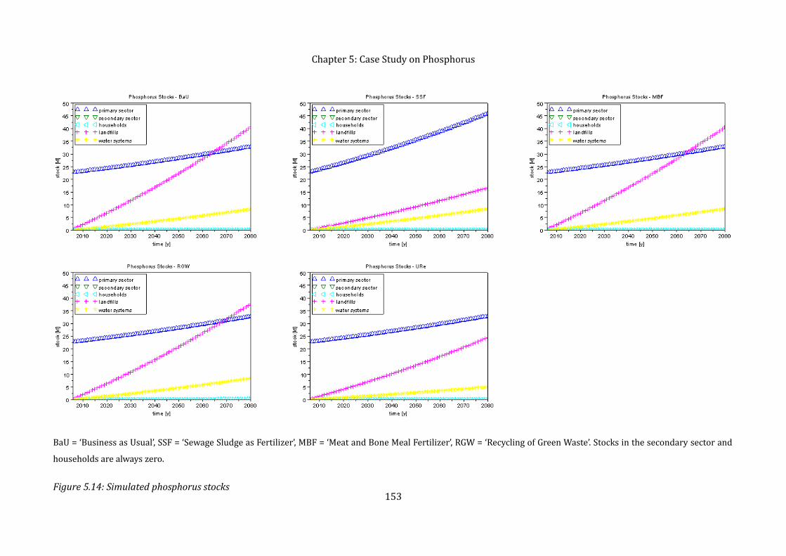
Chapter 5: Case Study on Phosphorus

153BaU = ‘Business as Usual’, SSF = ‘Sewage Sludge as Fertilizer’, MBF = ‘Meat and Bone Meal Fertilizer’, RGW = ‘Recycling of Green Waste’. Stocks in the secondary sector and households are always zero. Figure 5.14: Simulated phosphorus stocks

Chapter 5: Case Study on PhosphorusTable 5.4: Synthesis of phosphorus simulation results

Indicator/Scenario ‘Business as Usual’

‘Sewage Sludge as Fertilizer’

‘Meat and Bone Meal as

Fertilizer’

‘Recycling of Green Waste’

‘Urine Recycling’

Apparent consumption in 2080 [kt] 1.1 1.3 1.1 1.1 1.1Apparent consumption per capita [kg] 1.6 1.9 1.7 1.6 1.6Primary consumption in 2080 [kt] 0.95 0.78 0.95 0.91 0.63Primary consumption per capita [kg] 1.4 1.1 1.4 1.3 0.9Net imports in 2080 [kt] 0.97 0.81 0.98 0.93 0.65Cumulated net imports in 2080 [kt] 59 48 59 57 39RIR in 2080 [%] 15 65 16 20 70RER [%] 15 55 16 20 48In-use stocks in 2080 [kt] 33 46 33 33 33In-use stocks per capita in 2080 [kg] 48 67 48 48 48Phosphorus addition to landfills by 2080 [kt] 41 17 40 38 24Phosphorus addition to water systems by 2080 [kt] 8.4 8.4 8.4 8.4 5.0

154

Chapter 5: Case Study on Phosphorus5.5 Uncertainty Analysis5.5.1 MethodAn uncertainty analysis has also been performed on the dynamic MFA model. The goal of this analysis was to shed light on the uncertainty of the modelling results stemming from the uncertainty in the initial data and parameter values. The uncertainty analysis was performed in two steps: firstly, by determining the uncertainty of the initial data and, secondly, by studying the error propagation during the simulation. The uncertainty analysis was performed only for the ‘Business as Usual’ scenario; the results for the other scenarios were thought to be comparable. 5.5.1.1 Data UncertaintyThe initial Swiss study for phosphorus metabolism included error margins; however, after the study was scaled to the Geneva level, the fate of these error margins was not quite clear. It does not seem valid to downscale the error margins in the same manner as the data have been downscaled and, on the other hand, they cannot be left intact since the quantities of material flows on a federal level are not all comparable to the Canton of Geneva. It is also unclear whether the uncertainties in the Geneva data can be assumed independent since all the data has been obtained from the same study. The error margins for the initial data have therefore been redefined based on the work of Hedbrant & Sörme (2001) who define error margins not as ± values but in terms of magnitudes (denoted ‘*/’). The suitable order of magnitude for data obtained from a study on a national level downscaled to local level is proposed as */2—this corresponds to the uncertainty interval [X/2, 2X]. This approach to defining error margins is practical when the data cannot be assumed to be independent and the uncertainties do not follow a statistical distribution. The error margins are undoubtedly quite large but since no better data sources on the phosphorus metabolism in Geneva exist, this uncertainty must be accepted. 5.5.1.2 Error PropagationThe error propagation was studied by performing the simulations for the maximal and minimal initial values given by the defined error margins. These maximal and minimal values provide us with the range within which the simulation results should be situated.

155

Chapter 5: Case Study on PhosphorusThis provides us with a worst case analysis for uncertainties. The maximal and minimal values of various flows can be combined in many different manners; various scenarios that allow the exploration of different combinations were therefore defined. Not all possible combinations were studied (the total number of different flow combinations amounts to 217 = 131,072) but only those that would give the most extreme results. The 16 scenarios studied along with their maximal and minimal values are listed in Appendix C. 5.5.2 Results of the Uncertainty AnalysisThe results of the uncertainty analysis can be seen in Figures 5.15, 5.16, and 5.17. The import and export flows have only two possible trajectories whereas landfilled and recycled waste and the inflow to water systems have several possible evolutions (8 for landfilled and recycled waste and 16 for water systems). This number of scenarios for the addition to water systems stems from the fact that it is influenced simultaneously by the import and export flows, the waste flows as well as the run-off from the primary sector.

156The ‘water systems’ flow corresponds in the stock and flow model to f11 + f13. Figure 5.15: Uncertainty analysis, results for flows

Chapter 5: Case Study on PhosphorusThe defined uncertainty intervals are quite large: for instance, the year 2080 phosphorus imports range from about 1,100 t to 4,300 t (or almost quadruple). The behaviour of the phosphorus stocks also ranges from growth to diminution depending on the uncertainty scenario studied. A reduction is seen for instance when the exports attain their maximal value and the imports the minimal one, or when the input flows to the economic sectors are minimal and the outflows maximal. In reality, the stocks can, of course, never have a negative value.

However, it is not very probable that the flows should vary in opposite directions. The variation of the flows, all changing in the same direction, gives the following results for the year 2080: – Inputs vary from 1,100 t to 4,300 t.– Exports vary from 600 t to 2,400 t.– The quantity of recycled materials varies from 72 t to 290 t.

157

Figure 5.16: Uncertainty analysis, results for stocks

Chapter 5: Case Study on Phosphorus– Apparent consumption varies from 560 t to 2,200 t.– Stocks in the primary sector vary from to 16 kt to 66 kt.– Stocks in landfills vary from 20 kt to 81 kt.– Stocks in water systems vary from 4.2 kt to 17 kt. Thus, the maximal and minimal stock and flow values differ by a factor of 4. As our model behaves in an almost linear manner, the uncertainty ranges in the final values are almost the same as in the initial data (*/2). Studied in this manner, the uncertainty levels of our phosphorus study are revealed to be quite large and more precise input data would therefore be needed in order to obtain more reliable simulation results.

5.6 Discussion & ConclusionPhosphorus is a resource that is vital to food production where it cannot be substituted by any other element. Since substitution is not an option, phosphorus recycling, greater efficiency, and reduced phosphorus consumption are the only viable reserve-conserving 158

Figure 5.17: Uncertainty analysis, results for apparent consumption

Chapter 5: Case Study on Phosphorussolutions. Potential recycling methods include notably the use of human excreta as fertilizer while phosphorus recovery from waste water and run-off represents another possibility. However, the acceptability and the potential health impacts of urine and night soil recycling remain to be examined more closely and the procedure for phosphorus recovery from waste water is still being developed. On the other hand, various means have been imagined to decrease phosphorus consumption, including a (large-scale) transition to organic agriculture, promoting the consumption of vegetables and cereals as opposed to the consumption of meat, or the adoption of vertical farms (see, for example, Despommier 2009). A decrease in the consumption of meat would imply less energy consumption, less greenhouse gas emissions, less water and land use as well as less need for fertilizers. It might also help to ensure that the world population’s food needs are met, although it is often argued that the problem does not lie in the quantity of food but in its uneven distribution. A (nearly) complete transition to organic agriculture with techniques such as crop rotation, compost use, and biological pest control should also allow a major decrease in mineral fertilizer use. However, organic systems often have lower yields than conventional ones (Karak & Bhattacharyya 2011). In 2008, the Canton of Geneva contained about 12 organic farms, representing about 3% of the total of over 450 farms (OCSTAT 2011a; OCSTAT 2005b).In this chapter, the phosphorus metabolism in the Canton of Geneva in the coming decades has been analysed based on a normalized Swiss SFA study (FOEN 2009b). Several recycling scenarios based on the FOEN study as well as a urine recycling scenario were examined on the Geneva scale. According to the baseline scenario, the phosphorus consumption should continue to grow in the future following the population growth in the Canton; net imports attain nearly 1 kt in 2080, increasing by over 50% compared to 2006. The ‘Sewage Sludge as Fertilizer’ and ‘Urine Recycling’ scenarios offer the greatest opportunities to close the phosphorus loop in the Canton; however, their environmental and health impacts still need to be closely investigated. A worst-case uncertainty analysis was also performed for the dynamic phosphorus model. Due to the data normalization process, the uncertainty in the initial data as well as in the model results is quite important: in the worst case, the values of the baseline results could be either multiplied or divided by two, depending on whether the initial data values are over- or underestimated. The logical continuation of this study would therefore be to 159

Chapter 5: Case Study on Phosphorusestablish more accurate data on the phosphorus metabolism in the Canton in order to decrease the error margins of the dynamic simulation. As there are few existing statistics on the subject, this data collection and estimation would undoubtedly be a strenuous and time-consuming task.

160

Chapter 6: Case Study on WoodChapter 6 Case Study on WoodOur case study on wood begins with an introduction to wood use in Switzerland (Chapter 6.1). The wood metabolism in the Canton of Geneva is examined in Chapter 6.2 while a dynamic MFA model constructed to simulate the evolution of the Canton’s wood stocks and flows is presented in Chapter 6.3. The case study ends with a discussion and a conclusion (Chapter 6.4). 6.1 IntroductionWood is a renewable resource with a variety of uses, notably in energy generation, construction and furniture manufacturing, pulp and paper industry as well as in packaging. The wood consumption per capita has remained relatively stable in Switzerland, although there are some yearly variations (Schmithüsen 2003). The final wood uses in Switzerland include energy generation (47% waste recovery included), wood products (25%), and pulp and paper products (28%) (FOEN 2010a). Most wood produced in Swiss forests is used in furniture manufacturing while the rest is used as fuel or in industry (Schmithüsen 2003).Switzerland can be divided in to five different regions characterized by their climate and other geographical characteristics: the Jura, the Central Plateau, the Pre-Alps, the Alps, and the Southern Alps. The Canton of Geneva is located in the Central Plateau, characterized by denser population and less forest cover than other regions in Switzerland (Schmithüsen 2003). Forests cover today about 30% of the national territory in Switzerland and the forest surface continues to grow (FOEN 2011). However, the situation is very different in the densely populated Canton of Geneva where the question of sustainable use of wood resources becomes increasingly relevant. Wood and forests in Switzerland have been studied from many different environmental perspectives. Generic studies (see, for example, Schmithüsen 2003; FOEN 2009a; FOEN 2010a) and more detailed accounts of various important issues, such as the CO 2 impacts of forestry and timber industry (Taverna et al. 2007), exist. Regional studies have also been carried out on wood resources and sustainable regional management, notably in Davos (Vorlet 2003) and in the Olten-Oensingen-Zofingen region in the Swiss Lowlands (Müller 1998). However, wood metabolism as such is studied less frequently: on a European level, at least one study from the Netherlands can be found (Hekkert et al. 2000). Nevertheless,

161

Chapter 6: Case Study on Wooddata on wood flows can also be found indirectly in for instance phosphorus metabolism studies (see, for example, FOEN 2009b). A study on the potential energy uses of biomass (including wood and wood wastes) in the Canton of Geneva was also carried out recently; this study provides much needed data on the wood stocks and flows in the Canton. It should be noted that paper and cardboard have not been included in the scope of this study; the focus is solely on the metabolism of wood. This study begins by examining the wood metabolism in the Canton of Geneva (Chapter 6.2). Later, a dynamic wood metabolism model is constructed and used to simulate the evolution of wood use in the Canton of Geneva (Chapter 6.3). 6.2 Wood Metabolism in the Canton of GenevaThe forest surface of the Canton of Geneva is quite small compared to the Swiss average. Forests cover only 10% of the territory, a percentage that has remained stable in spite of environmental pressure (DIAE 2000). Oak is the main tree species present in the Canton as a result of clay soils and a warmer and drier climate than elsewhere in Switzerland (Canton of Geneva 2011d). The Canton’s forests are, however, of mediocre quality and of little economic interest: 90% of the wood production is in fact used for wood energy (DIAE 2000; Faessler et al. 2010). Slightly more than half (54%) of the Canton’s forests are state-owned (Faessler et al. 2010). The stocks and flows of wood have recently been studied in the Geneva agglomeration5 (Faessler 2011). The results of this study can be summarized briefly as follows (the units correspond to tonnes of fresh matter at 33% humidity): The Canton’s forest stocks stand at 413,000 t, whereas the annual wood harvest is 5,400 t. The annual amount of wood available to harvest is actually 12,100 t but 5,200 t are thought to be inaccessible; this leaves an unexploited potential of 1,500 t. About 90% (4,900 t) of the harvested wood is used as wood energy. The wood waste flows were also studied: 29,600 t of wood waste are used for energy via incineration in the Canton of Geneva whereas 6,400 t of non-dangerous wood waste are recycled outside the Canton. The recycling rate for material recovery thus stands at about 18%. The wood product imports from outside the Canton were not included within the scope of the study; however, they are implicitly present in the created waste flows. 5 The Geneva agglomeration includes the Canton of Geneva, the Nyon District in the Canton of Vaud as well as parts of the French Haute-Savoie and Ain departments.162

Chapter 6: Case Study on Wood

Wood metabolism has also been examined in an earlier metabolism study for the year 2000 (Faist Emmenegger & Frischknecht 2003); the findings of this study can be seen in Figure 6.1. According to this study, yearly wood imports (paper and cardboard excluded) amount to 37,500 t whereas local harvest stands at 4,200 t, and recycling inside the Canton provides 1,900 t; this gives us a total consumption of about 44 kt. The wood stocks in the three economics sectors and households are four times greater than the forest stocks. Households and the tertiary sector are the biggest wood users (representing 39% and 34% respectively) while the secondary and primary sectors follow. According to Faist Emmenegger and Frischknecht (2003), wood is mostly used in buildings and construction (58%) along with furniture (12%), packaging (11%), heating (10%), and woodwork (8%) in the secondary sector. According to the study, the annual consumption per capita is 12 kg 163

‘Wood Energy’ is here represented as a separate process although it is in reality integrated in the functioning of the economic sectors.Source: adapted from Faist Emmenegger & Frischknecht (2003). Figure 6.1: Wood metabolism in the Canton of Geneva in 2000

Chapter 6: Case Study on Woodor over a third less than the Swiss average (19 kg). Wood waste amounts to 27,000 t and about 55% of the wood waste (16,000 t) is collected for recycling purposes; the majority (13,000 t) of the recovered waste is exported to Italy while the rest is used as wood energy in the primary sector or incinerated.The amount of harvests in the Canton seems compatible across the two studies; however, the value given by the more recent study is about 23% higher than that of the earlier study (Faist Emmenegger & Frischknecht 2003; Faessler et al. 2010). The quantities of waste flows are also somewhat similar (27,100 t versus 36,000 t); nevertheless, the value of Faessler et al. (2010) is 25% higher. The quantity of recycled wood exports was estimated to be two times bigger in the earlier than in the later study (13,000 t versus 6,400 t respectively). There is an even greater discrepancy between the amounts of incinerated waste: 7,900 t versus 29,600 t. It should be noted that the wood consumption estimated by Faist Emmenegger and Frischknecht (2003) differs from the amount obtained in our phosphorus study by normalizing a Swiss phosphorus metabolism study to the Geneva level (Chapter 5.3). Faist Emmenegger and Frischknecht (2003) arrive at a total of 44 kt (including the consumption of recycled wood) while the normalized phosphorus study indicates an amount of 220 kt or five times as much. The Geneva study also indicates that wood energy represents only about 10% of wood use (Faist Emmenegger & Frischknecht 2003) while at the federal level in Switzerland this percentage has been estimated at 47%, paper and cardboard excluded (FOEN 2009c). It is not quite clear which data should be deemed more accurate: the Swiss average might not be representative of Geneva-related particularities whereas the data from the Faist Emmenegger and Frischknecht (2003) study are already 10 years old and might have quite large error margins. Moreover, data uncertainties are not explicitly provided. 6.3 Dynamic Modelling of Wood Metabolism6.3.1 Stock and Flow Model for Wood MetabolismThe wood metabolism in the Canton of Geneva was modelled using a dynamic stock and flow model (Figure 6.2). This dynamic model consists of:

164

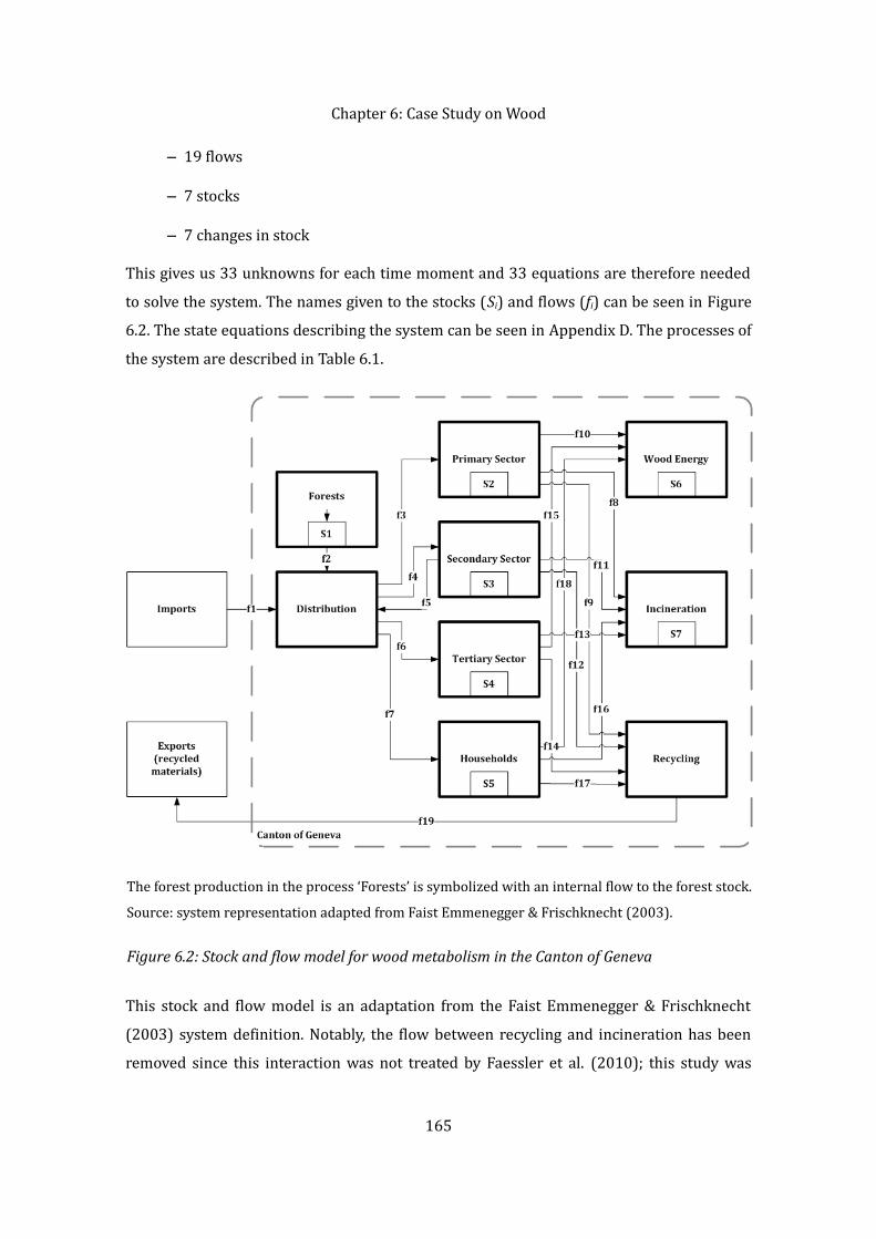
Chapter 6: Case Study on Wood– 19 flows– 7 stocks– 7 changes in stockThis gives us 33 unknowns for each time moment and 33 equations are therefore needed to solve the system. The names given to the stocks (Si) and flows (fi) can be seen in Figure6.2. The state equations describing the system can be seen in Appendix D. The processes of the system are described in Table 6.1.

This stock and flow model is an adaptation from the Faist Emmenegger & Frischknecht (2003) system definition. Notably, the flow between recycling and incineration has been removed since this interaction was not treated by Faessler et al. (2010); this study was 165

The forest production in the process ‘Forests’ is symbolized with an internal flow to the forest stock.Source: system representation adapted from Faist Emmenegger & Frischknecht (2003).Figure 6.2: Stock and flow model for wood metabolism in the Canton of Geneva

Chapter 6: Case Study on Woodused to supply most of the input values. The flow from recycling to the primary sector has also been removed for the same reasons. The ‘Wood Energy’ process represents the use of wood as wood energy in the various economic sectors.Table 6.1: Wood system processes

Process Name Process Description Change in StockImports Import of timber and wood products from outside the Canton -

Forests Forestry (wood production) in the Canton YesDistribution Distribution of recycled and harvested wood to the economic sectors NoPrimary Sector Use of wood in the primary sector (agriculture) YesSecondary Sector Use of wood in the secondary sector (industry, manufacturing) YesTertiary Sector Use of wood in tertiary sector (services) YesHouseholds Use of wood in households YesIncineration Incineration of wood waste in the Canton YesRecycling Collection and recycling of wood waste NoWood Energy Use of wood as fuel in the economic sectors YesExports (recycled materials) Export of wood waste to be recycled outside the Canton -

6.3.1.1 Precision on VocabularyThe following denominations are used:– Net imports correspond to the f1 flow.– Primary materials consumption corresponds to f1 – f19.– Apparent consumption corresponds to f1 + f2.

166

Chapter 6: Case Study on WoodThe Canton’s forest production is not taken into account in the primary wood consumption as the Canton’s production is thought to be ‘free’: only the wood that must be imported from outside the Canton will be taken into account. 6.3.1.2 Dynamic Behaviour of the SystemThe dynamic behaviour of the system is defined by the following assumptions:1. The apparent consumption follows population growth. The apparent wood consumption per capita is assumed to be constant. The used apparent consumption value and its source are presented in Chapter 6.3.2.2. The wood production in the Canton’s forests remains constant. The wood production values are obtained from Faessler et al. (2010).3. The relative sizes of individual import and export flows remain unchanged.The relative sizes of the import and export flows from various economic sectors were determined according to the Faist Emmenegger & Frischknecht (2003) study. 4. The waste flows follow the input flows with a given residence time distribution.The following section details the assumptions on the residence time distribution. The same residence time distribution was used for all the economic sectors. 5. The relative sizes of incinerated and recovered waste flows remain fixed in the economic sectors. 6. The wood used as wood energy is assumed to leave the economic sectors the same year it enters them. The total use of wood energy represents 47% of apparent consumption; the share of wood energy used in each economic sector is assumed to be fixed. The calculation of the amounts of wood energy, and incinerated and recovered waste in the economic sectors is explained in Chapter 6.3.2. 6.3.1.3 Residence TimeInstead of using a static residence time, I have chosen to model a residence time distribution which is undoubtedly a more realistic approach. There are many different distributions that are used to model product lifespans, for instance the Gaussian

167

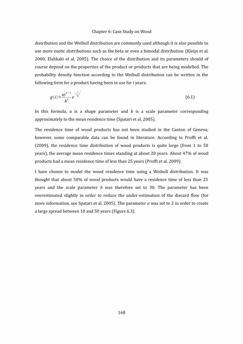
Chapter 6: Case Study on Wooddistribution and the Weibull distribution are commonly used although it is also possible to use more exotic distributions such as the beta or even a bimodal distribution (Kleijn et al. 2000; Elshkaki et al. 2005). The choice of the distribution and its parameters should of course depend on the properties of the product or products that are being modelled. The probability density function according to the Weibull distribution can be written in the following form for a product having been in use for i years:g i=aia−1

ba e− i

b

a (6.1)In this formula, a is a shape parameter and b is a scale parameter corresponding approximately to the mean residence time (Spatari et al. 2005). The residence time of wood products has not been studied in the Canton of Geneva; however, some comparable data can be found in literature. According to Profft et al. (2009), the residence time distribution of wood products is quite large (from 1 to 50 years), the average mean residence times standing at about 20 years. About 47% of wood products had a mean residence time of less than 25 years (Profft et al. 2009). I have chosen to model the wood residence time using a Weibull distribution. It was thought that about 50% of wood products would have a residence time of less than 25 years and the scale parameter b was therefore set to 30. The parameter has been overestimated slightly in order to reduce the under-estimation of the discard flow (for more information, see Spatari et al. 2005). The parameter a was set to 2 in order to create a large spread between 10 and 50 years (Figure 6.3).

168

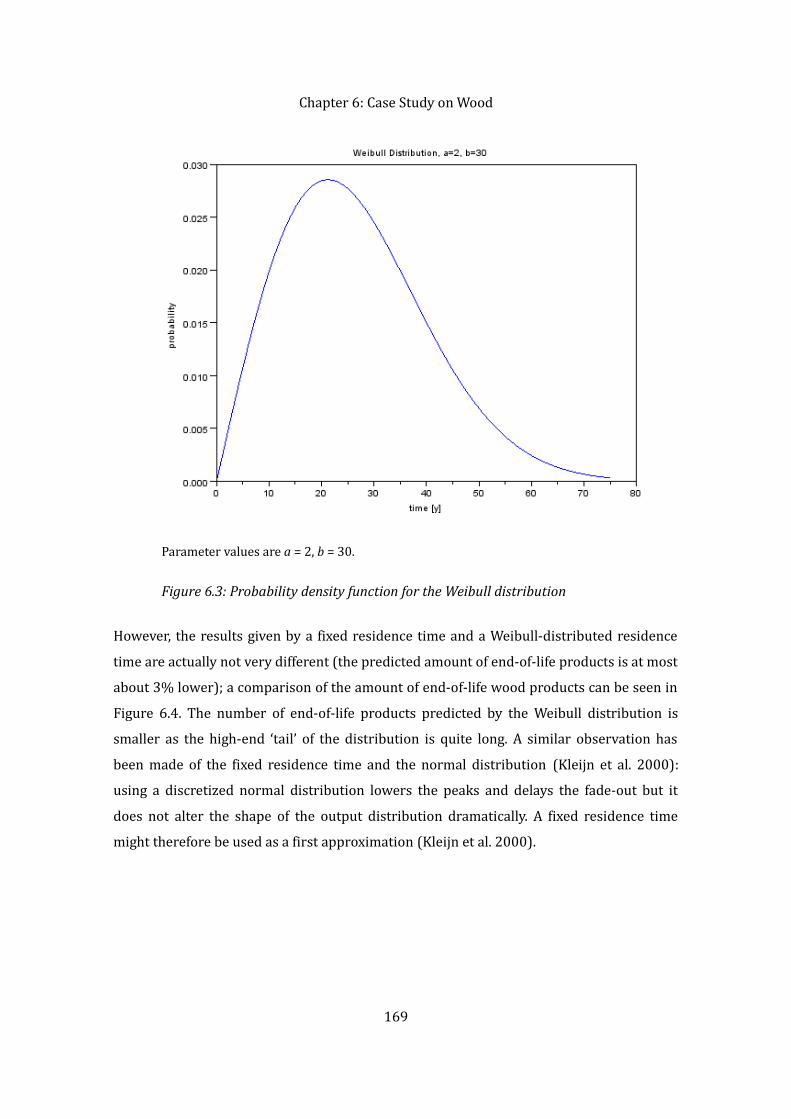
Chapter 6: Case Study on Wood

However, the results given by a fixed residence time and a Weibull-distributed residence time are actually not very different (the predicted amount of end-of-life products is at most about 3% lower); a comparison of the amount of end-of-life wood products can be seen in Figure 6.4. The number of end-of-life products predicted by the Weibull distribution is smaller as the high-end ‘tail’ of the distribution is quite long. A similar observation has been made of the fixed residence time and the normal distribution (Kleijn et al. 2000): using a discretized normal distribution lowers the peaks and delays the fade-out but it does not alter the shape of the output distribution dramatically. A fixed residence time might therefore be used as a first approximation (Kleijn et al. 2000).

169

Parameter values are a = 2, b = 30.Figure 6.3: Probability density function for the Weibull distribution

Chapter 6: Case Study on Wood

6.3.2 ScenariosThe dynamic MFA model has been used to study two different scenarios:– Business as Usual– Exploiting the Harvest PotentialThe scenarios have been composed by data provided by the two metabolism studies done in Geneva (the details on the data use and sources are given in Appendix D). In order to remain coherent with the phosphorus study (Chapter 5), the values of wood imports were calculated based on the normalized data of this study, giving nearly 220 kt. In order to convert the phosphorus value to wood quantity, it was divided by the phosphorus concentration or 0.06 g/kg (FOEN 2009b). The share of wood energy was thought to be 47% of the apparent consumption (or about 100 kt), in accordance with the Swiss average (FOEN 2009c). According to Faist Emmenegger and Frischknecht (2003), wood is used for heating purposes in Geneva in the primary and tertiary sectors and households. The values given by Faessler et al. (2010) were used for the total amounts of incinerated and

170

Figure 6.4: Comparison of results with a fixed residence time and a Weibull distribution

Chapter 6: Case Study on Woodrecovered wood waste as for the Canton’s wood harvest. The sectorial contributions to the waste flows were determined by using the sector weights from Faist Emmenegger & Frischknecht (2003). All the values of the baseline scenario are summarized in AppendixD. The ‘Potential’ scenario differs from the baseline scenario in the respect that the annual harvest values in Geneva’s forests are assumed to rise to the estimated maximum potential (6,900 t instead of the actual 5,400 t). The initial values used in the simulations are further detailed in Appendix D. The starting year of the simulation was chosen to be 2006; this was also the reference year of the Swiss phosphorus study (FOEN 2009b) However, part of the data from Faessler et al. (2010) is from 2008. Some data (notably the stock sizes in the economic sectors) are much less recent, dating back to 2000 (Faist Emmenegger & Frischknecht 2003).6.3.3 Model Results

6.3.3.1 Results after First Import EstimationThe evolution of the wood stocks and flows in the ‘Business as Usual’ scenario can be seen in Figures 6.5 and 6.6. When comparing the results given by the model and the data from Faessler et al. (2010) on the amount of wood waste, it becomes apparent that the waste amount predicted by the model is much too high. According to the model, the wastes (incinerated and recycled) amount to 91 kt in 2006 versus 36 kt according to Faessler et al. (2010); the model value is thus over 2.5 times too high. Small variations of wood residence time do not allow the removal of this difference and it was therefore decided that the initial value of the wood imports should be modified in order to obtain results that correspond better to the known waste values.

171

Chapter 6: Case Study on Wood

The import value was determined to be between 92,200 t and 97,100 t depending on whether the recycled or the incinerated waste flows should match the results of Faessler et al. (2010).6 For the following simulations, the weighted average of 96,200 t of wood imports was used. This value represents only about 44% of the originally used value (217,000 t, see Appendix D). When using the value of 96,200 t of wood imports, the Canton’s forest production represents 5.3% of the total wood consumption. Annual wood energy use in 2006 (fixed at 47% of the total wood consumption) now represents about 47,800 t.

6 In our dynamic MFA model, the proportion of recycled and incinerated waste was not fixed but depended on the sector outputs. For this reason, the recycling and incineration percentages do not match the results of Faessler et al. (2010) perfectly.172

Figure 6.5: Simulated wood flows, ‘Business as Usual’ scenario

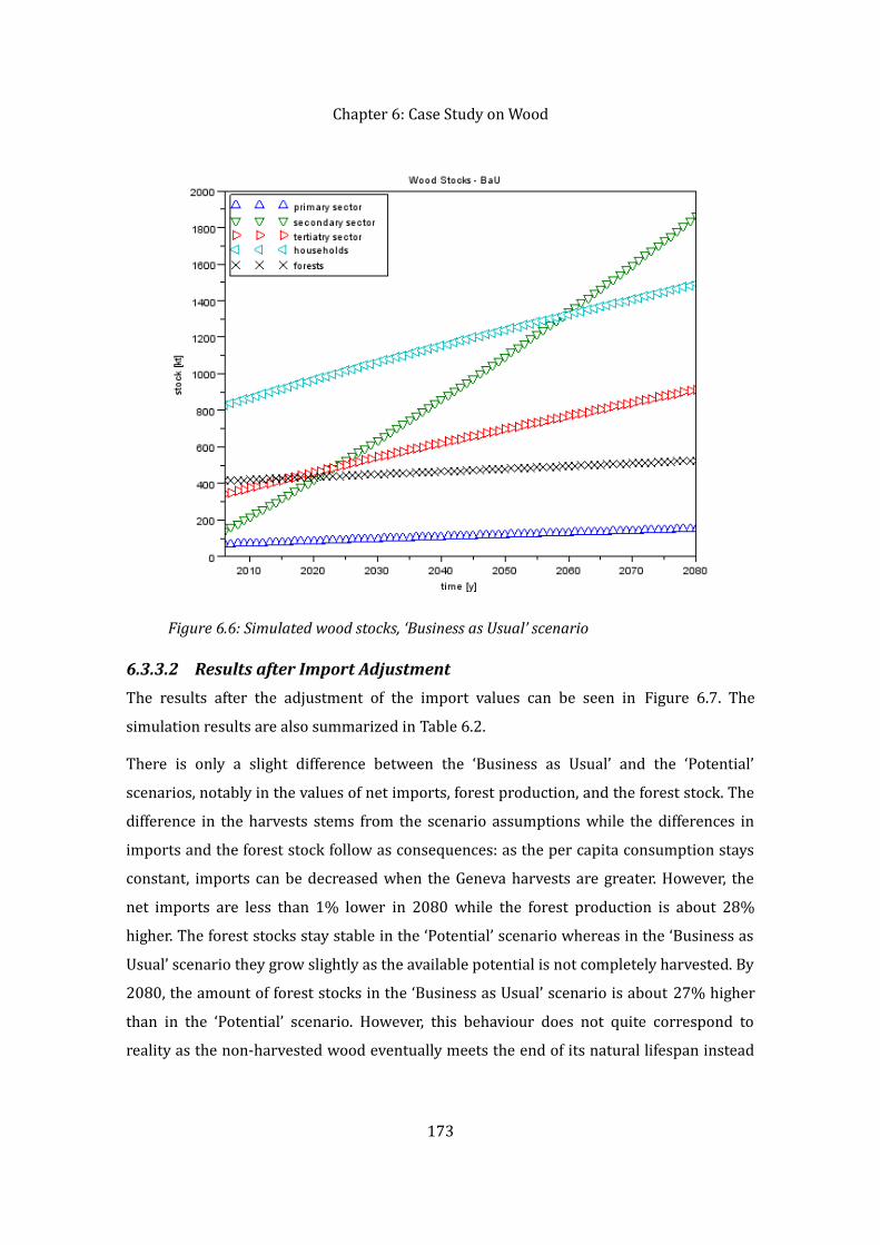
Chapter 6: Case Study on Wood

6.3.3.2 Results after Import AdjustmentThe results after the adjustment of the import values can be seen in Figure 6.7. The simulation results are also summarized in Table 6.2. There is only a slight difference between the ‘Business as Usual’ and the ‘Potential’ scenarios, notably in the values of net imports, forest production, and the forest stock. The difference in the harvests stems from the scenario assumptions while the differences in imports and the forest stock follow as consequences: as the per capita consumption stays constant, imports can be decreased when the Geneva harvests are greater. However, the net imports are less than 1% lower in 2080 while the forest production is about 28% higher. The forest stocks stay stable in the ‘Potential’ scenario whereas in the ‘Business as Usual’ scenario they grow slightly as the available potential is not completely harvested. By 2080, the amount of forest stocks in the ‘Business as Usual’ scenario is about 27% higher than in the ‘Potential’ scenario. However, this behaviour does not quite correspond to reality as the non-harvested wood eventually meets the end of its natural lifespan instead 173

Figure 6.6: Simulated wood stocks, ‘Business as Usual’ scenario

Chapter 6: Case Study on Woodof accumulating indefinitely in the forests. The forest stocks per capita decrease slightly over the simulation period as a result of population growth. The wood consumption (rising from about 100 kt in 2006 to 160 kt in 2080) as well as the recycling rates (19%) are identical in the two scenarios. The wood consumption thus increases about 7 kt per decade. The modelled recycling percentage differs lightly from that estimated by Faessler et al. (2010); this stems from the fact that the overall recycling percentage is not fixed in the model. The individual recycling rates in the economic sectors are fixed and the relative weights of the sectors are calculated based on their inflows. The secondary sector (where the recycling rate is 37%) has more weight than the primary sector (where the recycling rate is 12%), and the global recovery rate is thus somewhat higher. The in-use stocks in the various economic sectors continue to grow in the two scenarios; however, the stock in the secondary sector grows faster than the stocks in the other sectors. This stems from the fact that the secondary sector does not use any wood energy and the consumed wood thus accumulates as in-use stock. This behaviour is not quite realistic since packaging is an important wood use in this sector (Faist Emmenegger & Frischknecht 2003). The creation of product categories or using a shorter residence time in the secondary sector could help to make the model behaviour more realistic.

174

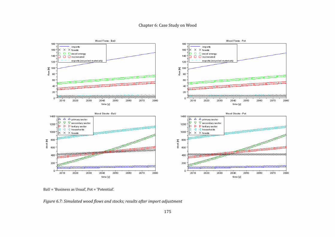
Chapter 6: Case Study on Wood

175BaU = ‘Business as Usual’, Pot = ‘Potential’.Figure 6.7: Simulated wood flows and stocks; results after import adjustment

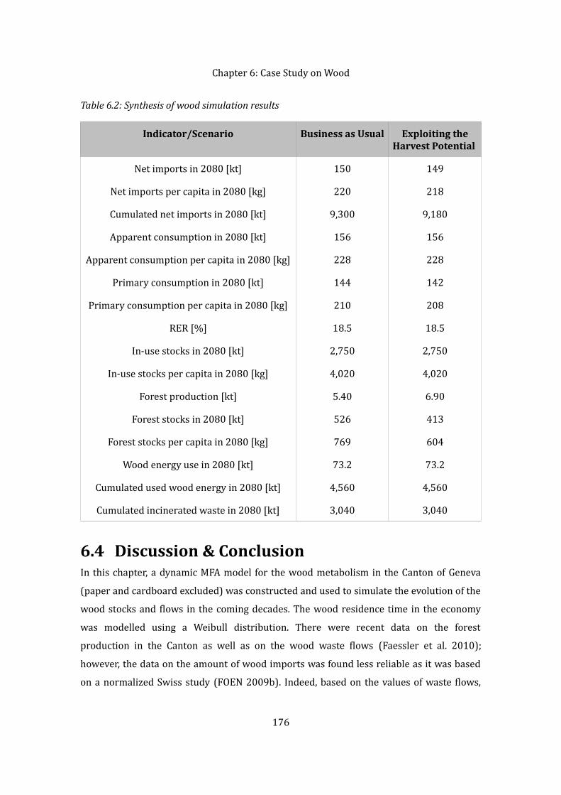
Chapter 6: Case Study on WoodTable 6.2: Synthesis of wood simulation results

Indicator/Scenario Business as Usual Exploiting the Harvest Potential Net imports in 2080 [kt] 150 149Net imports per capita in 2080 [kg] 220 218Cumulated net imports in 2080 [kt] 9,300 9,180Apparent consumption in 2080 [kt] 156 156Apparent consumption per capita in 2080 [kg] 228 228Primary consumption in 2080 [kt] 144 142Primary consumption per capita in 2080 [kg] 210 208RER [%] 18.5 18.5In-use stocks in 2080 [kt] 2,750 2,750In-use stocks per capita in 2080 [kg] 4,020 4,020Forest production [kt] 5.40 6.90Forest stocks in 2080 [kt] 526 413Forest stocks per capita in 2080 [kg] 769 604Wood energy use in 2080 [kt] 73.2 73.2Cumulated used wood energy in 2080 [kt] 4,560 4,560Cumulated incinerated waste in 2080 [kt] 3,040 3,040

6.4 Discussion & ConclusionIn this chapter, a dynamic MFA model for the wood metabolism in the Canton of Geneva (paper and cardboard excluded) was constructed and used to simulate the evolution of the wood stocks and flows in the coming decades. The wood residence time in the economy was modelled using a Weibull distribution. There were recent data on the forest production in the Canton as well as on the wood waste flows (Faessler et al. 2010); however, the data on the amount of wood imports was found less reliable as it was based on a normalized Swiss study (FOEN 2009b). Indeed, based on the values of waste flows, 176

Chapter 6: Case Study on Woodthe estimated import value was much too high and it was therefore corrected to correspond to the observed waste quantity before further analysis. The analysis of the defined scenarios (‘Business as Usual’ and ‘Exploiting the Harvest Potential’) revealed that although Geneva’s forest production could be more intensely exploited—almost 30% more wood could be harvested annually—this would only have a small impact on the amount of imported wood (a reduction of about 1% in 2080). In 2006, Geneva’s forest production represented only 5% of the wood consumed in the Canton according to our model results.In order to improve the accuracy of the wood metabolism model, it would be crucial to obtain more accurate data on the wood imports and their nature (wood products and/or wood energy). Recent estimations indicate that the amount of wood energy used in the Canton would be around 15,000 t of wood at 33% humidity (or 10,000 t of dry matter); this number corresponds to the capacity of installed boilers subsidized by the Canton’s energy service, ScanE, and an inter-communal energy management centre, CIME (Jérôme Faessler, Institute F.-A. Forel, University of Geneva, personal communication by email, 27 September 2011). This value is only a third of the one used in the simulations (47,800 t after adjustment); however, it is not clear how close the number of subsidized boilers is to the total number of boilers used in the Canton. Future improvements on the wood metabolism model could also include a more detailed modelling of the wood residence time: in this model, the same Weibull distribution was used for all the economic sectors. In order to devise more accurate sectorial residence time distributions, more data on the wood uses in these sectors is needed. Data on sectorial waste flows could also be of use when determining residence times. It would also be conceivable to model the wood growth and wood stock evolution in the Canton’s forests more accurately; however, as the focus of this thesis was on societal metabolism, this aspect was deemed outside the scope of this research.

177

178

Chapter 7: Case Study on LithiumChapter 7 Case Study on LithiumIn this chapter, the lithium needs in the Canton of Geneva are studied from an electric mobility (or e-mobility) perspective. A transition to electric mobility is an interesting topic as it would likely lead to a considerable increase in the Canton’s lithium demand. No quantitative metabolism model has been constructed as the values of the stocks and flows of lithium are yet to be studied; the magnitude of future lithium needs is however estimated with a few simple calculations.The chapter begins with a general introduction to lithium and its uses (Chapter 7.1), followed by an estimation of the development of lithium needs in the Canton of Geneva in an e-mobility context (Chapter 7.2). The case study ends with a short discussion and a conclusion (Chapter 7.3). 7.1 Introduction7.1.1 On the Importance of LithiumLithium is a relatively rare metal element that occurs in nature exclusively in compounds as a result of its high reactivity. Lithium is widely distributed on Earth but its concentration is often very low and its deposits small: the exploitation of lithium is thus economically feasible only at few locations (Garrett 2004). Lithium sources include rocks (in United States, Australia, and Zimbabwe), brines (Chile, Bolivia, and Argentina) as well as hectorite clays (United States) while seawater is also a major lithium source (Garrett 2004; Tahil 2008). Lithium reserves are estimated to amount to 13 Mt whereas lithium resources could be about 33 Mt (USGS 2011). Countries with the biggest reserves are currently Chile and China: the Chilean reserves (7.5 Mt) represent nearly 60% of the world total whereas the Chinese reserves (3.5 Mt) represent more than a quarter (USGS 2011). About 70% of the world’s deposits occur at one small location: the Lithium Triangle on the borders of Chile, Bolivia, and Argentina (Tahil 2008). This triangle is bounded by three lithium-rich salars or salt lake deposits: Salar de Atacama, Salar de Uyuni, and Salar de Hombre Muerto (Tahil 2008). Lithium is used, among other things, in batteries, lubricating greases, frits and glass, air conditioning, polymers, aluminium, pharmaceuticals, continuous casting, and chemical

179

Chapter 7: Case Study on Lithiumprocessing (Yaksic & Tilton 2009). Lithium is popular in batteries because of its hight electrochemical potential; this particular characteristic of lithium, its potential as an energy carrier, is a topic that is currently under much discussion. It is commonly thought that the biggest growth potential for lithium use lies in batteries, especially in rechargeable lithium-ion (Li-ion) batteries (USGS 2011). Rechargeable Li-ion batteries are currently used, for instance, in portable electronics such as laptop computers, mobile phones, and video cameras and, according to the US Geological Survey (USGS 2011), they have continued to gain market share over other battery types thanks to their high energy density. Major automobile companies pursue the development of lithium batteries for future hybrid vehicles, i.e. vehicles combining an internal combustion engine and an electric motor (USGS 2011). Li-ion batteries are also used in full electric vehicles (EVs) such as the Japanese Nissan Leaf (Nissan North America 2011). The benefits of EVs include a decrease in local pollution (no exhaust gases) and noise as well as a reduction in global green house gas emissions thanks to the efficiency of electric engines (De Decker 2010). One should, however, bear in mind that lithium is only an energy carrier, not an energy source and that it cannot replace oil in this sense; lithium vehicles still need to be powered by some external energy source. Consumers’ enthusiasm for electric cars is hampered by fears of being left stranded with a flat battery (Webster 2010). The development of a comprehensive charging infrastructure thus appears as a prerequisite for the breakthrough of e-mobility. Lithium recycling is currently not a viable economic solution, if the costs of lithium extraction and the costs of collecting and recycling lithium-containing batteries are compared (Hamilton 2009). In a recent study, the global lithium recycling rate was estimated at less than 1% (Graedel et al. 2011). In 2006, 20% of portable equipment batteries were recycled and the European Union Directive 2006/66/EC has fixed the target at 45% for 2016 (EC 2006), although there is no certainty that this Directive will be followed (Tahil 2008). Currently only materials like cobalt and nickel are recovered from recycled Li-ion batteries (Dewulf et al. 2010). However, at least one company is already starting to recycle lithium from used batteries (Toxco 2003).

180

Chapter 7: Case Study on Lithium7.1.2 Peak LithiumIt is estimated that the current lithium resource base of about 480 Gt contained in the Earth’s crust could last some 23 billion years at the current consumption rate (Yaksic & Tilton 2009). Using the USGS (2011) data for lithium reserves (13 Mt) and the current global production rate (25 kt), the reserve lifetime can still be estimated at over 500 years. The problem with lithium availability lies in the fact that lithium needs could grow very rapidly in the future as a result of a transition to electric mobility. At an annual growth rate of 3%, the current global lithium reserves would be depleted in 94 years and at a growth rate of 10% in merely 41 years.Strictly speaking, the peak of lithium actually refers to the peaking of easily-extractable, high-concentration lithium. The problem is once again not an absolute shortage of resources but the rarefaction of resources that can be exploited at a low energy and environmental cost. The amount of lithium in seawater has been estimated to 250 Gt; however, the lithium concentration in seawater is only 0.17 ppm or more than a hundred times less than in the Earth’s crust (Yaksic & Tilton 2009). South American salars have lithium concentrations that are more than 1,000–10,000 times greater (Tahil 2008). The amount of potentially recoverable lithium in seawater has been estimated to 45 Gt (Yaksic & Tilton 2009); however, the feasibility of its exploitation remains uncertain. The potential future evolution of lithium production and consumption has been analysed from an energy perspective in a recent Master’s Thesis (Carles 2010). According to the results of this work, the global lithium demand could be multiplied by 1.5 million if full e-mobility for passenger cars is achieved by 2100 and if the passengers per car ratio increases to three to one as a result of rising living standards (the ratio is currently only eight to one). This means that lithium reserves and resources could be depleted at a much more rapid pace. In a scenario studied by Yaksic & Tilton (2009), full e-mobility is expected to be achieved by 2050. 7.2 Lithium and the Canton of Geneva7.2.1 On E-MobilityIn 2010, there were 245,665 motor vehicles circulating in the Canton of Geneva (OCSTAT 2011d). The quantity of electric vehicles in Geneva can be assumed to be small since the total number of hybrid and full electric vehicles circulating in Switzerland is only about

181

Chapter 7: Case Study on Lithium11,500 (SFOE 2010). If the lithium content in a car battery is about 4 kg—this data corresponds to the Nissan Leaf (Althaus 2010)—this would mean that the amount of lithium required to replace all the internal combustion engine vehicles in Geneva by electric vehicles would be about 980 t or nearly 4% of the current global lithium production (USGS 2011). If all the Swiss vehicles, 5,273,297 in 2009 (FSO 2011b), were to be replaced with electric ones, this would require 21 kt of lithium or over 80% of the current annual world production (USGS 2011). Of course, in reality the replacement of internal combustion engine vehicles would not happen overnight but over a long period of time, probably spanning over several decades. When we look at the data on passenger cars, the results are similar: 4,009,602 vehicles of this category circulate in Switzerland (FSO 2011b) requiring a total of 16 kt of lithium for batteries (Althaus 2010). In Geneva, the number of passenger cars is 214,444 (OCSTAT 2011d)—their replacement would therefore require about 860 t of lithium (Althaus 2010). It is difficult to put these numbers into perspective on the Geneva level as there is no data on the Canton’s lithium consumption. On Swiss level, electric vehicles represent less than 0.3% of passenger vehicles; in the case of a 100% transition to electric mobility, the amount of lithium contained in passenger vehicle batteries would thus be multiplied by nearly 350. 7.2.2 Available Lithium Sources As there are no economically viable lithium deposits in Switzerland, all lithium must be imported from abroad. This could become somewhat problematic as lithium is not without its geopolitical issues (similarly to oil): as stated earlier, 70% of lithium reserves are controlled by Chile, Bolivia, and Argentina (Tahil 2008). There could be a potential risk of price- and production-controlling cartel formation (Carles 2010). As a basis for comparison, 12 OPEC member countries hold collectively nearly 80% of the world’s crude oil reserves (BP 2010).Because of these geopolitical issues, lithium extraction from seawater, where lithium is only present in low concentration, has been studied and R&D investments have been made, notably in South Korea (Kim 2010). Lithium extraction from seawater remains expensive due to its high energy requirements but if a breakthrough technology were to allow a reduction in energy requirements by two orders of magnitude, lithium would be available for hundreds of thousands of years (Carles 2010). In South Korea, a commercial

182

Chapter 7: Case Study on Lithiumlithium extraction plant should be operational by 2015 and its capacity should be large enough to replace all lithium carbonate imports (Kim 2010). Investments in seawater extraction could also be envisioned in Switzerland (although the country does not have its own coastline). Different types of extraction technologies exist, for instance lithium can be extracted directly from seawater (as in the Korean technology) while it might also be possible to extract lithium from the waste brines created by desalination plants. However, the energy requirements of lithium extraction from seawater need to be lowered by two orders of magnitude in order to become economically feasible (Carles 2010).7.2.3 Closing the Lithium CycleIn addition to imported lithium, recycled lithium could also be an attractive source. Indeed, as metals consumption has increased, there has been a continuous shift from metal stocks in the lithosphere to metals stocks in the anthroposphere; metal in-use stocks have also been called ‘anthropogenic mines’ (Gerst & Graedel 2008). However, as lithium recycling is not economically viable on a very small scale, this option might not be profitable on a cantonal scale. Recycling could perhaps be organized on a national or European level, especially when the quantities of discarded lithium batteries become larger. It has been shown that starting to recycle batteries now at a global level could save about 20 years’ worth of low energy cost lithium (Carles 2010). It is therefore important to start recycling as soon as possible to delay future shortages. 7.3 Discussion & ConclusionIn this thesis, a brief analysis of the various issues concerning lithium and its metabolism in the Canton of Geneva was carried out. The main problem in analysing the lithium metabolism is that there is little actual data on the lithium stocks and flows. Data collection should therefore be organized, for instance on Swiss federal level. Only when more data or at least more accurate estimations are available, would it be possible to perform a true substance flow analysis for lithium. Another problem related to lithium metabolism is that the estimation of future lithium needs remains very difficult: this difficulty is notably related to the question of e-mobility. Will electric mobility make its great breakthrough? And will the future EVs be powered by lithium-containing batteries? At the moment, the answer to the second question seems likely to be yes while the first point remains yet unclear. These uncertainties make all

183

Chapter 7: Case Study on Lithiumfuture projections fairly unreliable; however, various potential evolutions could be analysed in the form of scenarios when (and if) a dynamic MFA model is constructed. Lithium recycling currently remains costly but it seems a good investment target in order to save primary lithium resources. However, in order to be economically viable, the recycling would need to be organized on a supranational level. Lithium extraction from seawater is another potential alternative; but once again, there is a great need for investment in the research and development phase in order to lower the energy consumption and thus the costs of lithium recovery from seawater as well as its environmental impacts. Nevertheless, one thing is clear: trading the dependence on oil for a dependence on lithium is not a truly sustainable solution. Lithium might only be a transition technology and the true solution thus lies in diversifying our energy storage (and energy source) solutions (Carles 2010).

184

Chapter 8: Case Study on Space Life Support SystemsChapter 8 Case Study on Space Life Support SystemsThis chapter present the case study on space life support systems. The chapter begins with an introduction to life support in space (Chapter 8.1) and the heart of the matter, modelling the sustainability of space life support systems, is presented in Chapter 8.2. The modelling section focuses on the comparison of two life support systems, ARES and BIORAT, in terms of the sustainability of resource use. The case study ends with a conclusion and a discussion on the limits of the comparison (Chapter 8.3). 8.1 Introduction8.1.1 On Life Support in SpaceSpace life support systems are systems that enable the survival of human beings in space. A life support system (LSS) must supply the crew with oxygen, water, and food; it can also be used, among other things, to regulate the cabin temperature, pressure, and humidity, and to dispose of carbon dioxide, solid, and liquid waste. Life support systems can be technical, chemical, or biological, or a combination of different types of technologies. The purpose of a life support system is to ensure the survival of the crew for the duration of the mission; the system must therefore be viable or sustainable—in the engineering sense of the word—during the entire mission.A typical crew member requires a total of approximately 15 kg of food, water, and oxygen per day to perform the standard activities on a space mission (Christophe Lasseur, ESA, personal communication, 7 January 2010). The required input is significantly smaller (only about 5 kg) when water for hygienic purposes is excluded (Christophe Lasseur, ESA, personal communication, 7 January 2010). The outputs consist of a similar amount of materials in the form of solid and liquid wastes, and carbon dioxide. The mass breakdown of these metabolic parameters is shown in Table 8.1. The oxygen consumption levels vary significantly depending on the activity level of the crew members.

185

Chapter 8: Case Study on Space Life Support SystemsTable 8.1: Daily needs of the crew and waste creation

Needs Quantity [kg/day/person]

Wastes Quantity[kg/day/person]O2 1 CO2 1Water total 3 Liquid waste 12Dry food 1 Perspiration and breathing 2Hygiene water 10 Dry solid waste 0.1TOTAL 15 TOTAL 15*

*The waste values do not quite add up due to rounding.Source: Jean Brunet, Sherpa Engineering and Christophe Lasseur, ESA (personal communication, 7 January 2010). In order to meet the crew needs, a complete life support system consists of three subsystems: an air revitalization system, a water recycling system, and a food production system. These three systems can be completely separate, loosely linked, or tightly interwoven. Space life support systems can be either physico-chemical or biological; biological life support systems also known as artificial ecosystems are presented in the following section. 8.1.2 Artificial EcosystemsArtificial ecosystems are artificial recreations of the Earth’s material cycle and its atmosphere in limited space and controlled conditions and within immediate time horizons (ESA 2007b). Artificial ecosystems are designed to recycle materials (various metabolic wastes) autonomously utilizing only the energy inputs provided. The focus of recycling is particularly on carbon, hydrogen, oxygen, nitrogen, sulphur, and phosphor (elements C, H, O, N, S, and P) which constitute 95% of matter to be recycled (ESA 2007b). However, in reality the presence of various trace elements must also be taken into account. The objective of artificial ecosystems is to recycle matter with the greatest possible efficiency.Contrary to natural ecosystems, the aim of artificial ecosystems is to reduce the number of material cycle interactions to a strict minimum and to dimension and control the different

186

Chapter 8: Case Study on Space Life Support Systemscompartments of the system in order to optimize their functioning with respect to defined objectives (ESA 2007b). In natural ecosystems, the stability of the system is ensured by a great number of populations interacting through feedback loops and relying on self-regulation.An example of an artificial ecosystem is the MELiSSA (Micro-Ecological Life Support System Alternative) ecosystem. The particularity of MELiSSA is that it is solely based on biological compartments. The MELiSSA material cycle (ESA 2006) is defined by five major compartments:– the consumer compartment (V)and four recycling compartments:– thermophilic anaerobic bacteria compartment (I)– photoheterotrophic bacteria compartment (II)– nitrifying bacteria compartment (III)– photosynthetic bacteria compartment (IVa) and higher plant compartment (IVb)In reality, the MELiSSA ecosystem is much more complex; the previously described five compartments correspond in fact to hundreds of physico-chemical or biological operations with approximately 150 different gas, liquid, and solid material flows involving over 30 constituents (ESA 2007b). For more information on the MELiSSA project, see, for example, the MELiSSA homepage (ESA 2006).

8.1.3 Characteristics of Space Life Support SystemsWhat is striking about space life support systems—when thought to include the entire spacecraft or station—is their isolation. In this aspects, life support systems could be compared to isolated islands or to the Earth system as a whole: interaction with the external environment is limited and the resources within the system are the only ones readily available. However, the situation changes when resources can be extracted from the extraterrestrial environment (e.g. Mars).According to Deschenes and Chertow (2004), islands are confronted with the problems of limited available resources and fragile resource security as well as a strictly limited carrying capacity of the environment. While all human populations come across these 187

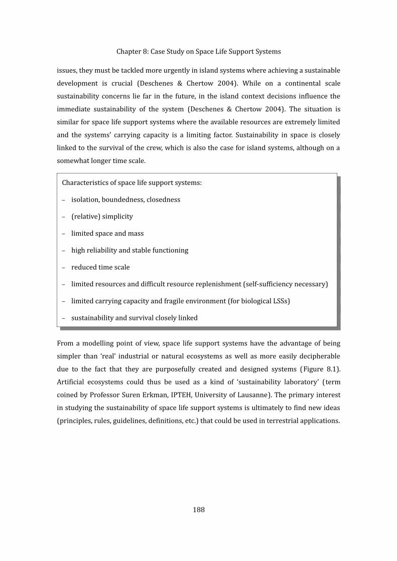
Chapter 8: Case Study on Space Life Support Systemsissues, they must be tackled more urgently in island systems where achieving a sustainable development is crucial (Deschenes & Chertow 2004). While on a continental scale sustainability concerns lie far in the future, in the island context decisions influence the immediate sustainability of the system (Deschenes & Chertow 2004). The situation is similar for space life support systems where the available resources are extremely limited and the systems’ carrying capacity is a limiting factor. Sustainability in space is closely linked to the survival of the crew, which is also the case for island systems, although on a somewhat longer time scale.Characteristics of space life support systems:– isolation, boundedness, closedness– (relative) simplicity– limited space and mass– high reliability and stable functioning– reduced time scale– limited resources and difficult resource replenishment (self-sufficiency necessary)– limited carrying capacity and fragile environment (for biological LSSs)– sustainability and survival closely linked

From a modelling point of view, space life support systems have the advantage of being simpler than ‘real’ industrial or natural ecosystems as well as more easily decipherable due to the fact that they are purposefully created and designed systems (Figure 8.1). Artificial ecosystems could thus be used as a kind of ‘sustainability laboratory’ (term coined by Professor Suren Erkman, IPTEH, University of Lausanne). The primary interest in studying the sustainability of space life support systems is ultimately to find new ideas (principles, rules, guidelines, definitions, etc.) that could be used in terrestrial applications.

188

Chapter 8: Case Study on Space Life Support Systems

8.1.4 Presentation of ARES and BIORATThis case study analyses two life support systems—ARES and BIORAT—which were the focus of the ALISSE Phase II project financed by ESA.ARES (Air REvitalisation System) is a chemico-technical life support system whereas BIORAT represents a biological life support system. Both ARES and BIORAT are limited to air revitalization: their main mission is to provide the crew with oxygen. Human oxygen needs vary depending on physical activity level but the average human respiratory quotient is about 0.87 (Laurent Poughon, Laboratoire de Génie Chimique et Biochimique, Université Blaise Pascal, personal communication by email, 26 June 2009). The respiratory quotient QR is defined as follows (ESA 2007c):QR=

CO2 produced [mol]O2consumed [mol] (8.1)The oxygen production quotient of a LSS is correspondingly defined as (ESA 2007c):

QP=O2produced [mol]CO2 consumed [mol] (8.2)

189

Figure 8.1: Industrial and natural ecosystems

Chapter 8: Case Study on Space Life Support SystemsAssuming that the quantities of produced and consumed oxygen are equal and that QRQP > 1, there will be an accumulation of carbon dioxide in the system: consumers are producing more CO2 than the system can absorb. This is the general difficulty in artificial ecosystems and it contributed notably to the failure of the Biosphere 2 experiment. The functions performed by an air revitalization system include notably (Tailhades 2008):– particle removal– volatile organic compound (VOC) removal– NH3 removal– CO2 removal– O2 concentration control– relative humidity (RH) control– temperature control– pressure control

8.2 Modelling the Sustainability of Space Life Support Systems8.2.1 ObjectivesThe objective of the case study was to evaluate and compare the functioning of the ARES and BIORAT systems in regard to the sustainability of resource use. In order to compare the two systems, a generic stock and flow representation for life support systems was defined (Chapter 8.2.2). Based on this generic model, material flow analyses were done for the two systems (Chapter 8.2.3). In order to interpret the results in terms of sustainability, it was necessary to define various sustainability indicators based on the material stocks and flows (Chapter 8.2.4). And finally, a simulation model was built for the two systems based on the information obtained from the (preliminary) material flow analyses, the simulation settings were defined, and the performances of the two systems were compared (Chapters 8.2.5―8.2.7).

190

Chapter 8: Case Study on Space Life Support SystemsThe objective of the case study was to evaluate and to compare the functioning of ARES and BIORAT in terms of resource use. The following steps were taken to achieve the objective:– Defining a generic stock and flow model for life support systems;– Establishing preliminary material flow analyses for ARES and BIORAT;– Defining sustainability indicators for life support systems; and– Building a simulation model for resource use in the ARES and BIORAT systems.

The steps taken to construct the life support system simulation model are explained schematically in Figure 8.2.

191

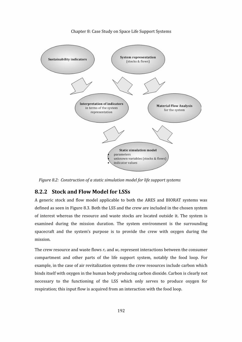
Chapter 8: Case Study on Space Life Support Systems

8.2.2 Stock and Flow Model for LSSsA generic stock and flow model applicable to both the ARES and BIORAT systems was defined as seen in Figure 8.3. Both the LSS and the crew are included in the chosen system of interest whereas the resource and waste stocks are located outside it. The system is examined during the mission duration. The system environment is the surrounding spacecraft and the system’s purpose is to provide the crew with oxygen during the mission.The crew resource and waste flows rc and wc represent interactions between the consumer compartment and other parts of the life support system, notably the food loop. For example, in the case of air revitalization systems the crew resources include carbon which binds itself with oxygen in the human body producing carbon dioxide. Carbon is clearly not necessary to the functioning of the LSS which only serves to produce oxygen for respiration; this input flow is acquired from an interaction with the food loop.192

Figure 8.2: Construction of a static simulation model for life support systems

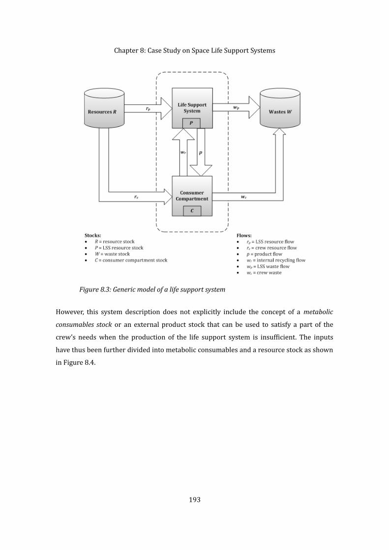
Chapter 8: Case Study on Space Life Support Systems

However, this system description does not explicitly include the concept of a metabolic

consumables stock or an external product stock that can be used to satisfy a part of the crew’s needs when the production of the life support system is insufficient. The inputs have thus been further divided into metabolic consumables and a resource stock as shown in Figure 8.4.

193

Figure 8.3: Generic model of a life support system

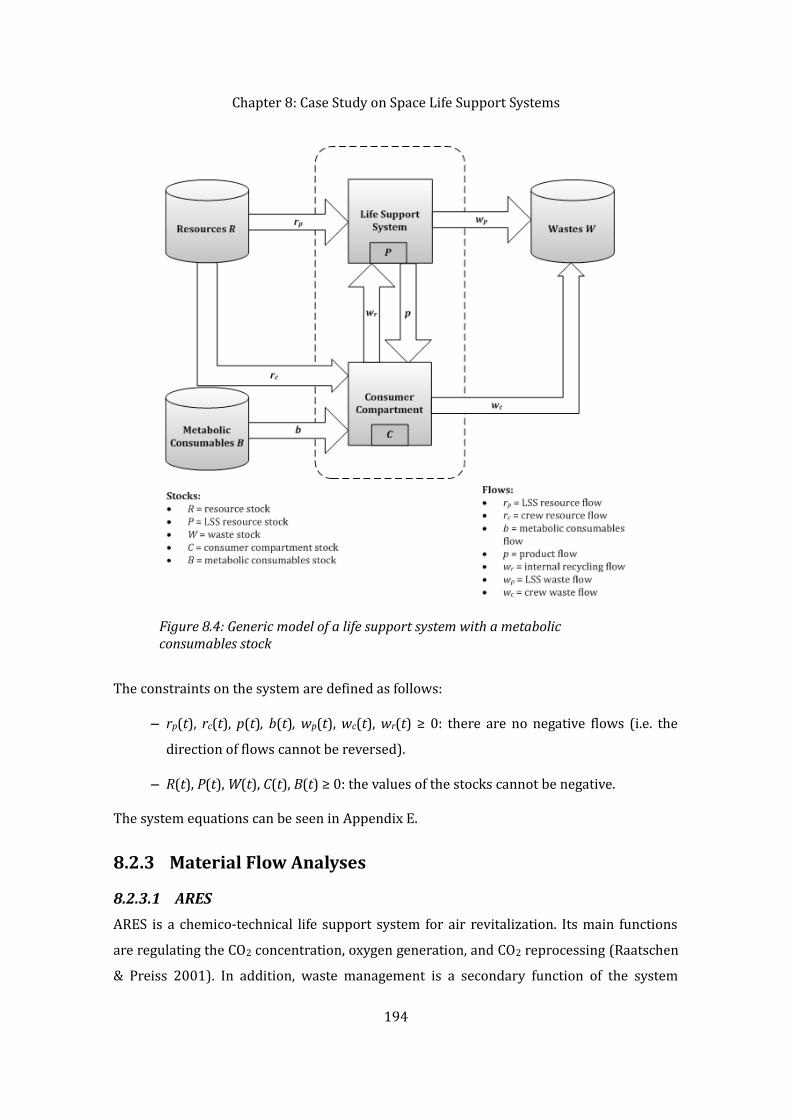
Chapter 8: Case Study on Space Life Support Systems

The constraints on the system are defined as follows:– rp(t), rc(t), p(t), b(t), wp(t), wc(t), wr(t) ≥ 0: there are no negative flows (i.e. the direction of flows cannot be reversed).– R(t), P(t), W(t), C(t), B(t) ≥ 0: the values of the stocks cannot be negative.The system equations can be seen in Appendix E.

8.2.3 Material Flow Analyses

8.2.3.1 ARESARES is a chemico-technical life support system for air revitalization. Its main functions are regulating the CO2 concentration, oxygen generation, and CO2 reprocessing (Raatschen & Preiss 2001). In addition, waste management is a secondary function of the system 194

Figure 8.4: Generic model of a life support system with a metabolic consumables stock

Chapter 8: Case Study on Space Life Support Systems(Raatschen & Preiss 2001). Oxygen generation is done by means of electrolysis and carbon dioxide reprocessing is handled in a Sabatier reactor. The ARES system is to be tested on-board the International Space Station.The material flow analysis for ARES is based on data obtained from the ALISSE II project prime contractor Sherpa Engineering (Olivier Gerbi, Sherpa Engineering, personal communication, 9 July 2008). The data is summarized in Figure 8.5. The key parameters of the reference mission were– a crew of seven individuals– one-year period– oxygen needs of 0.85 kg/day/personThe amounts of oxygen and carbon dioxide transmitted to and from the crew compartment correspond to a respiratory quotient of 0.87. The goal of the system is to provide a crew of seven individuals with oxygen during one year. According to Jean Brunet from Sherpa Engineering (2009), the ARES system operates around a given sizing point, i.e. a predetermined level of oxygen production, and the production cannot be adapted in accordance with consumer needs.

195

Chapter 8: Case Study on Space Life Support Systems

Based on this information, the values of various stocks and flows of materials in the system can be calculated. The results of the material flow analysis are presented in Figure 8.6. This representation is based on the generic LSS stock and flow diagram (Figure 8.4). In analysing the material balances of the system, it became apparent that the amount of carbon and oxygen inputs did not match the amount of outputs from the consumer compartment. These ‘missing’ flows are marked in italics (Figure 8.6). It has been assumed that these flows result from an undefined interaction of the human metabolism with the food subsystem which is not included within the scope of our analysis. The oxygen production quotient QP (Equation 8.2) obtained for this system is about 2.0. The energy consumption of ARES was estimated to 1.659 MJ/mole O2 (Jean Brunet, Sherpa Engineering, personal communication by email, 3 February 2010).

196

Source: Olivier Gerbi, Sherpa Engineering (personal communication, 9 July 2008).Figure 8.5: ARES schema of principle

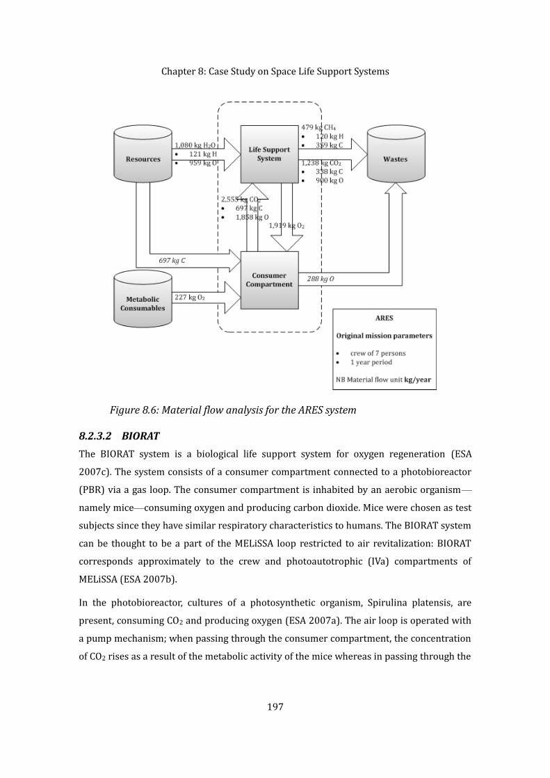
Chapter 8: Case Study on Space Life Support Systems

8.2.3.2 BIORATThe BIORAT system is a biological life support system for oxygen regeneration (ESA 2007c). The system consists of a consumer compartment connected to a photobioreactor (PBR) via a gas loop. The consumer compartment is inhabited by an aerobic organism—namely mice—consuming oxygen and producing carbon dioxide. Mice were chosen as test subjects since they have similar respiratory characteristics to humans. The BIORAT system can be thought to be a part of the MELiSSA loop restricted to air revitalization: BIORAT corresponds approximately to the crew and photoautotrophic (IVa) compartments of MELiSSA (ESA 2007b).In the photobioreactor, cultures of a photosynthetic organism, Spirulina platensis, are present, consuming CO2 and producing oxygen (ESA 2007a). The air loop is operated with a pump mechanism; when passing through the consumer compartment, the concentration of CO2 rises as a result of the metabolic activity of the mice whereas in passing through the 197

Figure 8.6: Material flow analysis for the ARES system

Chapter 8: Case Study on Space Life Support Systemsphotobioreactor, CO2 is transformed into oxygen in order to revitalize the atmosphere of the consumer compartment (Figure 8.7).

The simplified equation of photosynthesis taking place in the photobioreactor can be written approximately as follows (Laurent Poughon, Laboratoire de Génie Chimique et Biochimique, Université Blaise Pascal, personal communication by email, 24 July 2009):1.0 CO2 + 0.2 HNO3 + 0.8 H2O → 1.0 CH1.8O0.4N0.2 + 1.5 O2 (8.3)In the photosynthetic reaction, carbon dioxide is converted into biomass while producing oxygen. Biomass is represented as CH1.8O0.4N0.2 and HNO3 represents the nutrient input required for biomass growth. This is obviously a simplification of the real situation since, for instance, the elements phosphorus (P) and sulphur (S) are not taken into account. The oxygen production quotient or the photosynthetic quotient QP (Equation 8.2) obtained for the BIORAT system in this simplified situation is 1.5 which is somewhat high: this stems 198

Source: ESA (2007c).Figure 8.7: BIORAT schema of principle

Chapter 8: Case Study on Space Life Support Systemsfrom the formula of the biomass (ibid). Photosynthetic quotient values obtained in simulation tests have been in the range of 1.29–1.39 (ibid). In the BIORAT system, the oxygen production can be rapidly adapted to consumer needs; the oxygen consumption of the mice depends largely on their activity level.The material flow analysis for the BIORAT system is based on information obtained from a BIORAT expert, Laurent Poughon from Université Blaise Pascal (personal communication by email, 25 June 2009) and from the BIORAT simulator of Sherpa Engineering (Jean Brunet, personal communication by email, 29 June 2009). The results are summarized in Figure 8.8. There have been various BIORAT test settings but the following reference mission will be focused on here:– crew of two mice– one-month period– oxygen needs of 3.455 g/day/mouseThe input of the PBR is nutrients (HNO3) and the outputs are biomass (CH1.8O0.4N0.2) as well as a small amount of carbon dioxide dissolved in liquid—this is a simplification of the actual photobioreactor. The respiratory quotient was fixed to 0.87 in order to enable comparisons to ARES with human users; the oxygen needs of two mice were assumed to be 9.0 mmol/h or 6.91 g/day (Doulami et al. 2005). This permits us to determine the amount of CO2 created by respiration: 7.83 mmol/h or 8.27 g/day.

199

Chapter 8: Case Study on Space Life Support Systems

The system was assumed to require 0.55 g of biomass to produce 1 g of O2 (Laurent Poughon, Laboratoire de Génie Chimique et Biochimique, Université Blaise Pascal, personal communication by email, 25 June 2009). For simplification purposes, the growing biomass is assumed to be continuously removed from the system, i.e. there is no growth in the stocks within the production system. The amount of nutrient inputs was calculated in accordance with the biomass quantity (especially in accordance with the nitrogen needs). The photosynthetic quotient obtained for the system is about 1.3; this value will be used later in the simulations. In order to balance the inputs and outputs, it is assumed that there is some interaction between the human metabolism and the food loop in the consumer compartment (Figure8.8, values marked in italics). This interaction corresponds approximately to the values obtained for ARES. However, there is also a problem on the photobioreactor level: an additional input of H and O is needed to balance the inputs and outputs (Figure 8.8, values marked in italics). It is assumed that this discrepancy stems from an interaction with the 200

Figure 8.8: Material flow analysis for the BIORAT system

Chapter 8: Case Study on Space Life Support Systemswater loop in the PBR. It is assumed that no stock accumulation occurs either in the photobioreactor or in the consumer compartment.The energy consumption of BIORAT was estimated to be 15.7 MJ/mole O2 assuming the use of LEDs with 25% efficiency and an intensity of 20 W/m2 (Jean Brunet, Sherpa Engineering, personal communication by email, 3 February 2010; information based on the calculations of Jean-François Cornet, Laboratoire de Génie Chimique et Biochimique, Université Blaise Pascal).8.2.4 Defining Sustainability IndicatorsIn order to analyse the sustainability of resource use, it is necessary to define indicators to measure it. Indicators that attempt to to characterize various life support system characteristics have been defined here. The chosen indicators are divided into four categories: 1. overall burden of the system in terms of materials and energy2. recycling and material use efficiency3. coverage time and need coverage level4. resource and waste intensity indicatorsSome of these indicators (direct material input, processed output, recovery rate of used products, material use efficiency, and use rate of recovered used products) are inspired from material flow accounting (Eurostat 2001; Hashimoto et al. 2004; OECD 2008c). The indicators adapted from Hashimoto et al. (2004) are further illustrated in Figure 8.9 for ARES.7

7 The material use time (MUT) indicator is not taken into account since it is identical for ARES and BIORAT systems; its value depends solely on the human metabolism.201

Chapter 8: Case Study on Space Life Support Systems

The sustainability indicators can be expressed in terms of stock and flow definitions from the system representation (Figure 8.4).The overall burden of the system in terms of mass and energy over the entire mission (T stands here for the duration of the mission) is expressed in the form of the following indicators:– direct material input, or R0 + B0 – processed output, or WT – W0 – total mass of the production system– total energy consumption of the production system

Recycling—recovery of used products—and material use efficiency (in discrete time) over the entire mission can be expressed as:– material use efficiency, or

202

Source: adapted from Hashimoto et al. (2004) and OECD (2008c).Figure 8.9: Adaptation of MFA indicators for ARES

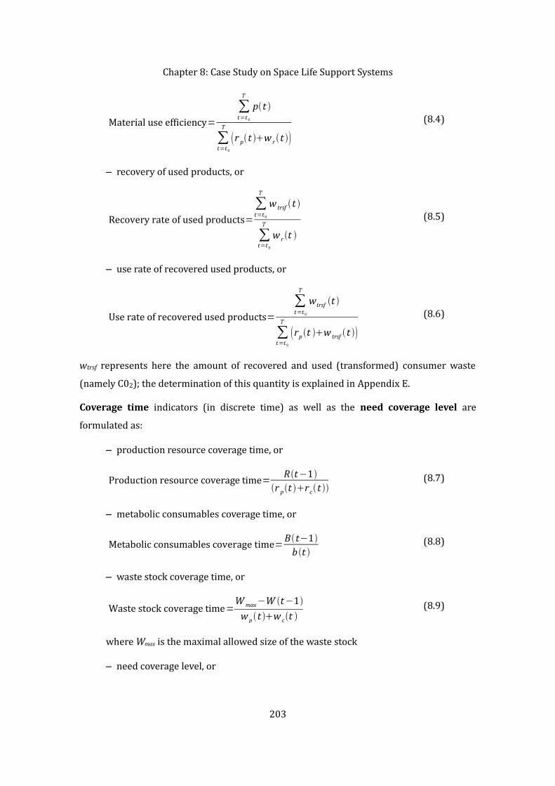
Chapter 8: Case Study on Space Life Support SystemsMaterial use efficiency= ∑

t=t 0T

pt

∑t=t 0

T

r pt w r t (8.4)

– recovery of used products, orRecovery rate of used products=∑t=t 0

T

w trsf t

∑t=t 0

T

w r t

(8.5)– use rate of recovered used products, orUse rate of recovered used products= ∑

t=t 0T

wtrsf t

∑t=t 0

T

rp t w trsf t (8.6)

wtrsf represents here the amount of recovered and used (transformed) consumer waste (namely C02); the determination of this quantity is explained in Appendix E.Coverage time indicators (in discrete time) as well as the need coverage level are formulated as:

– production resource coverage time, orProduction resource coverage time= Rt−1

r pt rct (8.7)

– metabolic consumables coverage time, orMetabolic consumables coverage time=Bt−1

b t (8.8)

– waste stock coverage time, orWaste stock coverage time=W max−W t−1

w pt w ct (8.9)

where Wmax is the maximal allowed size of the waste stock– need coverage level, or

203

Chapter 8: Case Study on Space Life Support SystemsNeed coverage level= ∑

t=t 0T

pt

∑t=t 0

T

pt b t

(8.10)Resource and waste intensity indicators for the production process have been defined as:

– resource intensity, or Resource intensity=∑t=t 0

T

rp t

∑t=t 0

T

pt

(8.11)– waste intensity, orWaste intensity=∑t= t0

T

w p t

∑t=t 0

T

pt

(8.12)The first category of indicators (mass and energy burden of the system) should be used to compare two systems only if the reference missions (mission duration, crew number, and oxygen needs) are identical. It is assumed that the two input stocks are greatest at t0 whereas the waste stock is at its greatest at T.The recycling and material use efficiency indicators can to some extent be used to compare systems of different dimensions. These indicators are here defined globally for the entire mission duration; however, they could also be calculated for each period t.The coverage time indicators are defined as dynamic indicators, evolving over time. Stock values at t – 1 (instead of values at t) are used because these values are thought to represent the stock size at the beginning of period t. The need coverage level can be understood as the objective of the system; for instance, in the case of BIORAT, the aim of the system is to cover 100% of consumer needs.Resource and waste intensity indicators—expressing the quantity of resources needed and waste created in the production of one unit of product—are here defined over the entire duration of the mission. Resource intensity is generally speaking a measure of the

204

Chapter 8: Case Study on Space Life Support Systemsresources (such as water, energy, or materials) needed for the production, processing, and disposal of a unit of good or service; it is therefore a measure of the efficiency of resource use. Resource intensity is here defined as the amount of primary (i.e. non-recycled) resources needed to produce one product unit. Waste intensity, on the other hand, is defined as the total of waste created in producing one unit of product. The waste intensity indicator is linked to material use efficiency; the following relation applies:Waste intensity= 1Material use efficiency −1 (8.13)

8.2.5 Constructing the Simulation ModelBased on the generic LSS representation (Figure 8.4) and the five system equations in discrete time (Appendix E) a simulation model can now be built. The system equations contain 11 unknown variables (5 stocks and 6 flows); 6 additional equations are therefore needed in order to solve the system.Let us assume that the system is in a steady state, i.e. the inputs of the production and consumption compartments equal the outputs. There is thus no material accumulation within the system.r pt w r t =pt w p t (8.14)rct bt pt =wr t wct (8.15)

Let us also assume that the needs of the crew must at all times be satisfied either by the metabolic consumables stock or by the LSS production:pt bt =n t (8.16)

n(t) equals the needs of the crew at period t. These needs are assumed to be known.Several system design parameters that contain information on the basic functioning of the system have also been defined. These design parameters are:– need coverage level NC, orNC=

pt pt b t

(8.17)– production resource intensity RIp, or

205

Chapter 8: Case Study on Space Life Support SystemsRI p=

rpt pt

(8.18)– consumer resource intensity RIc, orRI c=

rc t pt bt

(8.19)– consumer waste intensity WIc, orWIc=

w ct pt bt

(8.20)The values of these design parameters are assumed to be known at each period t; they can be either constant or time dependant. These four parameters are not the only options, it would also be possible to fix other suitable design parameters. The need coverage level and resource intensity parameters are related to previously defined sustainability indicators (Equations 8.11 and 8.12); however, they are defined for period t instead of an average for the entire mission.With regard to ARES and BIORAT, the numerical values of the static design parameters can be obtained from the material flow analysis results. These design parameters together with the steady-state equations (Equations 8.14―8.15), the need satisfaction equation (Equation 8.16), and the system equations allow us to determine the values of the stock and flow variables (see Appendix E for more details).8.2.6 Simulations Settings The behaviour of ARES and BIORAT can now be simulated with the defined simulation model. The simulations were carried out for the total mass flow of the system as well as for the oxygen element. The model cannot be directly used for the elements C, H, and N since the chosen design parameters cannot be defined when some of the flows are zero.The simulation model was in practice implemented as an Excel spreadsheet with sections for input parameters, outputs, and indicators. There were both common and simulation-specific input parameters: the common parameters included crew size, mission duration, and oxygen needs whereas the design parameters were specific to the oxygen and total mass simulations. The ‘need coverage level’ design parameter was assumed to be a

206

Chapter 8: Case Study on Space Life Support Systemsmodifiable operating parameter, whereas the other design parameters were considered fixed.The results for the static simulations in discrete time for one time period (one day) are shown in Appendix E. Assuming the situation remains static, the flow values will remain the same for all the simulation periods while the input stocks steadily diminish and the waste stock grows.Similar simulation models can be constructed for other elements circulating in the system. For ARES, these elements are carbon and hydrogen, and for BIORAT carbon, hydrogen, and nitrogen. These elements are not present in all the system flows which leads to certain simplifications and to some differences in the design parameters that need to be defined. For example, in the BIORAT model nitrogen is only found in the production system inputs and outputs (flows rp and wp)—therefore, only a design parameter determining the amount of nitrogen required to produce the desired amount of oxygen is needed.8.2.6.1 Design Parameter ValuesThe values of the chosen system design parameters—need coverage level, resource intensities, and waste intensity—first need to be defined in order to solve the stock and flow values for ARES and BIORAT. These design parameters were calculated using information obtained from the material flow analyses (Chapter 8.2.3); the design parameter values were assumed constant. It was also assumed that the initial and maximal stock values should match the resource and waste storage needs:

R0=∑t=t0

T

r p t rct (8.21)B0=∑

t=t 0T

bt (8.22)W max=W 0∑

t=t 0T

w p t wc t (8.23)The initial stocks of the production system, P0, of the consumer compartment, C0, as well as of the external waste storage, W0, were thought to be zero. The values of the production system mass were unknown and were therefore left blank.

207

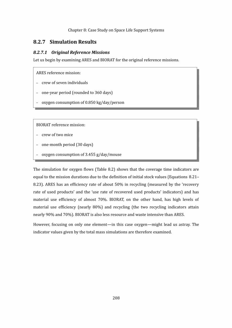
Chapter 8: Case Study on Space Life Support Systems8.2.7 Simulation Results

8.2.7.1 Original Reference MissionsLet us begin by examining ARES and BIORAT for the original reference missions.ARES reference mission:– crew of seven individuals– one-year period (rounded to 360 days)– oxygen consumption of 0.850 kg/day/personBIORAT reference mission:– crew of two mice– one-month period (30 days)– oxygen consumption of 3.455 g/day/mouse

The simulation for oxygen flows (Table 8.2) shows that the coverage time indicators are equal to the mission durations due to the definition of initial stock values (Equations 8.21–8.23). ARES has an efficiency rate of about 50% in recycling (measured by the ‘recovery rate of used products’ and the ‘use rate of recovered used products’ indicators) and has material use efficiency of almost 70%. BIORAT, on the other hand, has high levels of material use efficiency (nearly 80%) and recycling (the two recycling indicators attain nearly 90% and 70%). BIORAT is also less resource and waste intensive than ARES.However, focusing on only one element—in this case oxygen—might lead us astray. The indicator values given by the total mass simulations are therefore examined.

208

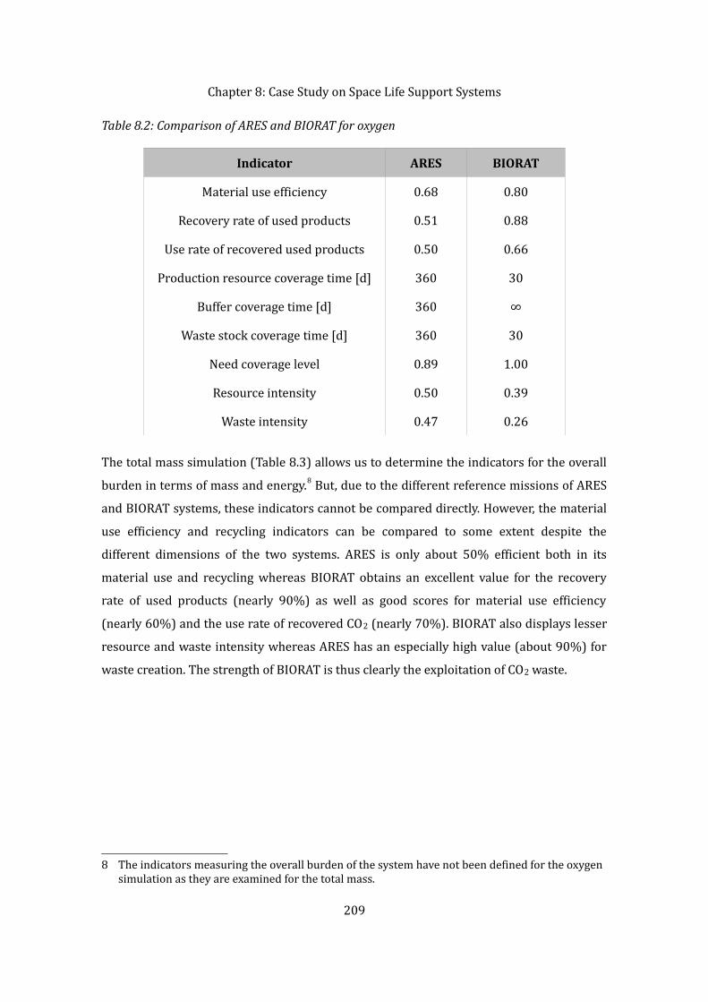
Chapter 8: Case Study on Space Life Support SystemsTable 8.2: Comparison of ARES and BIORAT for oxygen

Indicator ARES BIORATMaterial use efficiency 0.68 0.80Recovery rate of used products 0.51 0.88Use rate of recovered used products 0.50 0.66Production resource coverage time [d] 360 30Buffer coverage time [d] 360 ∞Waste stock coverage time [d] 360 30Need coverage level 0.89 1.00Resource intensity 0.50 0.39Waste intensity 0.47 0.26The total mass simulation (Table 8.3) allows us to determine the indicators for the overall burden in terms of mass and energy.8 But, due to the different reference missions of ARES and BIORAT systems, these indicators cannot be compared directly. However, the material use efficiency and recycling indicators can be compared to some extent despite the different dimensions of the two systems. ARES is only about 50% efficient both in its material use and recycling whereas BIORAT obtains an excellent value for the recovery rate of used products (nearly 90%) as well as good scores for material use efficiency (nearly 60%) and the use rate of recovered CO2 (nearly 70%). BIORAT also displays lesser resource and waste intensity whereas ARES has an especially high value (about 90%) for waste creation. The strength of BIORAT is thus clearly the exploitation of CO2 waste.

8 The indicators measuring the overall burden of the system have not been defined for the oxygen simulation as they are examined for the total mass.209

Chapter 8: Case Study on Space Life Support SystemsTable 8.3: Comparison of ARES and BIORAT for total mass

Indicator ARES BIORATDirect material input [kg] 2000 0.17Processed output [kg] 2000 0.17Total mass of the production system [kg] - -Total energy consumption of the system [MJ] 310 3.4Material use efficiency 0.53 0.59Recovery rate of used products 0.51 0.88Use rate of recovered used products 0.55 0.68Production resource coverage time [d] 360 30Buffer coverage time [d] 360 ∞Waste stock coverage time [d] 360 30Need coverage level 0.89 1.00Resource intensity 0.56 0.50Waste intensity 0.89 0.70

210

Chapter 8: Case Study on Space Life Support Systems8.2.7.2 Identical Reference MissionsIt is interesting to compare ARES and BIORAT for identical reference missions. It is assumed here that the BIORAT system could be redimensioned to match ARES; the common reference mission was chosen to correspond to the original ARES mission (crew of seven, one-year period, oxygen needs of 0.850 kg/day/person). The purpose of this thesis is not to estimate whether this redimensioning could be done and what changes it might impose; the aim was merely to illustrate the differences in the resource use of ARES and BIORAT. It is assumed that ARES relies partly on an external oxygen stock (as in the original material flow analysis) whereas BIORAT produces all the required oxygen without requiring a metabolic consumables stock.

The oxygen simulations for the two systems can now be directly compared (Table 8.4) as well as the total mass simulations (Table 8.5); these results are visualized in Figure 8.10. Most indicator values remain unchanged when the reference mission is changed—they are not dependent on the system dimensioning—except for the total mass and energy burden 211

Figure 8.10: Comparison of ARES and BIORAT in terms of total mass and oxygen flows

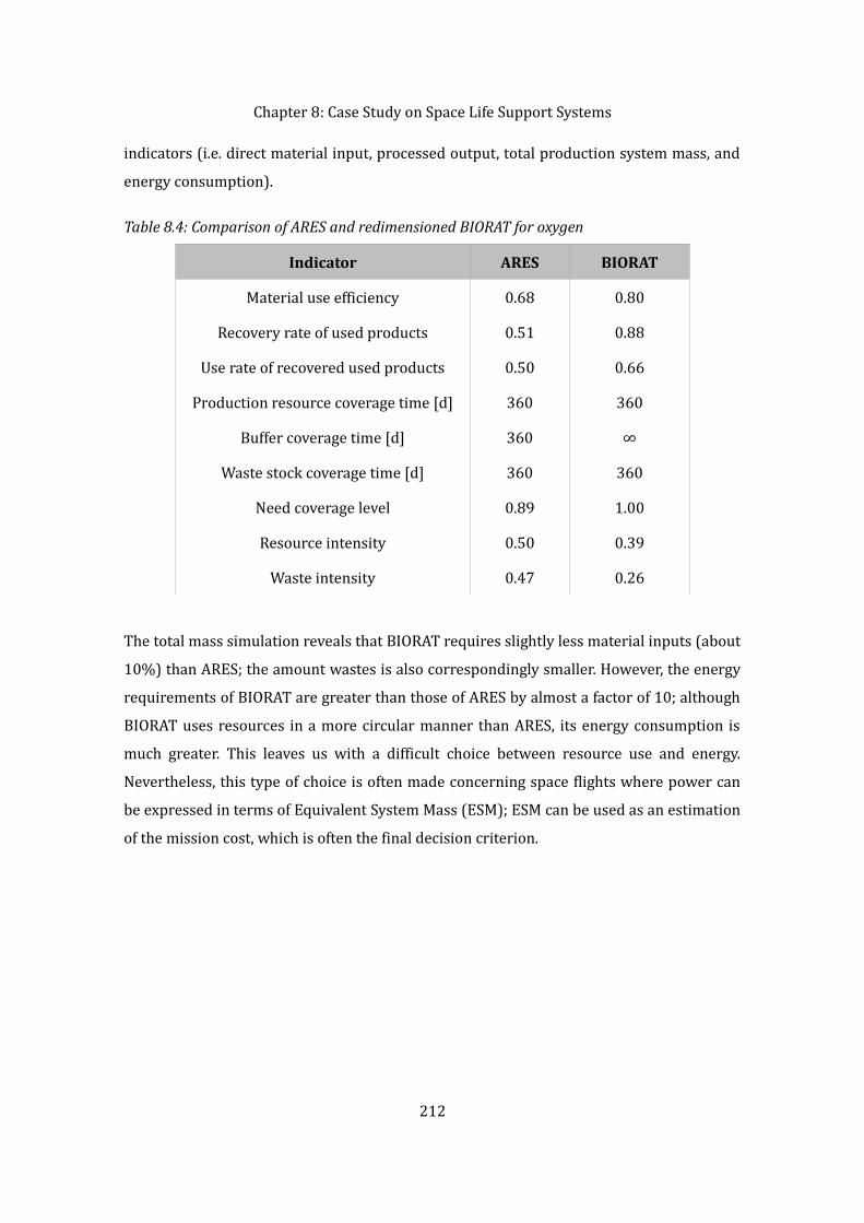
Chapter 8: Case Study on Space Life Support Systemsindicators (i.e. direct material input, processed output, total production system mass, and energy consumption).Table 8.4: Comparison of ARES and redimensioned BIORAT for oxygen

Indicator ARES BIORATMaterial use efficiency 0.68 0.80Recovery rate of used products 0.51 0.88Use rate of recovered used products 0.50 0.66Production resource coverage time [d] 360 360Buffer coverage time [d] 360 ∞Waste stock coverage time [d] 360 360Need coverage level 0.89 1.00Resource intensity 0.50 0.39Waste intensity 0.47 0.26The total mass simulation reveals that BIORAT requires slightly less material inputs (about 10%) than ARES; the amount wastes is also correspondingly smaller. However, the energy requirements of BIORAT are greater than those of ARES by almost a factor of 10; although BIORAT uses resources in a more circular manner than ARES, its energy consumption is much greater. This leaves us with a difficult choice between resource use and energy. Nevertheless, this type of choice is often made concerning space flights where power can be expressed in terms of Equivalent System Mass (ESM); ESM can be used as an estimation of the mission cost, which is often the final decision criterion.

212

Chapter 8: Case Study on Space Life Support SystemsTable 8.5: Comparison of ARES and redimensioned BIORAT for total mass

Indicator ARES BIORATDirect material input [kg] 2000 1800Processed output [kg] 2000 1800Total mass of the production system [kg] - -Total energy consumption of the system [MJ] 310 2900Material use efficiency 0.53 0.59Recovery rate of used products 0.51 0.88Use rate of recovered used products 0.55 0.68Production resource coverage time [d] 360 360Buffer coverage time [d] 360 ∞Waste stock coverage time [d] 360 360Need coverage level 0.89 1.00Resource intensity 0.56 0.50Waste intensity 0.89 0.708.2.7.3 Comparison of Oxygen ProductionIt is also possible to compare the origins of the oxygen consumed by the crew: the oxygen must come either from an external metabolic consumables stock or from the production system as recycled oxygen or as ‘new’ oxygen obtained from input resources (Figure 8.11). The oxygen from recycling is defined as

Oxygen from recycling= ∑t= t0

T

w r t

∑t=t 0

T

w rt r pt pt (8.24)

and the oxygen from resource stocks as

213

Chapter 8: Case Study on Space Life Support SystemsOxygen from resource stocks= ∑

t= t0T

r p t

∑t=t 0

T

w r t r p t pt (8.25)

This analysis confirms that BIORAT derives its oxygen largely from recycling (70%) whereas ARES relies slightly more on external oxygen inputs either through the production system (30%) or directly from the oxygen stock (about 10%).

8.3 Discussion & ConclusionIn this chapter, the sustainability of two space life support systems, ARES and BIORAT, were evaluated and compared. In order to do this, indicators to measure the sustainability of resource use in space life support systems were first defined and, secondly, material flow analyses were performed for the systems under study. Based on the results of the material flow analyses, static simulation models were constructed for the two systems and their behaviour was compared using both the original mission parameters and the parameters of a common reference mission. BIORAT outperforms ARES in terms of all the 214

Figure 8.11: Comparison of daily oxygen production

Chapter 8: Case Study on Space Life Support Systemsdefined indicators except for energy consumption: it requires nearly 10 times as much energy as ARES to produce the same quantity of oxygen. ARES and BIORAT are by nature very different types of systems: the oxygen production level of ARES is fixed and cannot be modified whereas BIORAT can be operated in a flexible manner in accordance with consumer needs. It is also unclear whether all the functions performed by the two systems (humidity and pressure control, removal of particles, etc.) are completely identical.Given that there are interactions with other life support subsystems (the food loop and the water loop), it seems awkward to exclude these systems from the initial material flow analyses. Ideally, all life support subsystems (air, water, and food loop) should be analysed at the same time in order to avoid problems in the definition of the system boundaries.It might also be noted that no information is available on the evolution of the systems and their behaviour; therefore, only simulations where the system inflows and outflows remain static can be performed. One might however assume that there is a degradation in performance over time and that this degradation could perhaps be more radical for a biological than for a technical life support system; it would therefore be interesting to include this dynamic aspect in the analysis.

215

Thesis Structure

PART IVRECOMMENDATIONS AND

CONCLUSION

218

Chapter 9: Policy for Sustainable Resource ManagementChapter 9 Policy for Sustainable Resource Management9.1 IntroductionOn a global level, resource consumption and pressure on world resources is expected to continue to increase in the future as a result of population growth and a rise in living standards. The global population is expected to increase by 50% in the first half of the 21st century (United Nations 2011). Were the material conditions of developing countries to approach those of the developed world, global resource consumption could be multiplied by a factor of two to five (EEA 2005). World economic growth has remained at around 3% annually over the past 30 years; this growth still remains linked to materials consumption although some relative decoupling has been achieved in developed countries (EEA 2005). However, many developing countries have entered the initial, resource-intensive phase of industrialization only recently or are set to do so in the near future. In particular, the continued industrialization of large economies (notably China) will significantly increase resource consumption and the pressure on the environment although some opportunities for technological ‘leapfrogging’ through technology transfer exist (EEA 2005).In the face of growing global demand and problems of resource availability, there is an urgent need to formulate a strategy leading towards sustainable resource use globally, as well as locally in the Canton of Geneva. Sustainable resource management (SRM) is an activity whose task is to ensure the long-term supply of materials and energy in an environmentally sustainable manner (Bringezu 2002). Sustainable resource management plays an important part in establishing a sustainable societal metabolism whose preconditions can be defined as follows (Bringezu 2002):

– Keeping flow values within the capacities of the environment; this concerns both resource extraction from the environment and the output of emissions and wastes into it;– Limiting the physical economic growth in order to achieve long-term sustainability of human societies with respect to the natural environment;– Achieving intragenerational equity: the benefits as well as the downsides of environmental resource use (extracted resources and land use as well as the

219

Chapter 9: Policy for Sustainable Resource Managementemissions of pollutant and waste) should be equally distributed in per capita terms; and – Achieving intergenerational equity: the opportunities of future generations should not be compromised by the resource use of the current one.The first two preconditions relate to the size of the physical economy and its stocks and flows whereas the last two are more qualitative requirements related to the social issues of sustainable development. Regarding sustainable use of natural resources and waste management, the objectives of the 6th Environment Action Programme have been formulated in the following manner by the European Commission (EC 2001):To ensure that the consumption of renewable and non-renewable resources and the associated impacts do not exceed the carrying capacity of the environment and to achieve a decoupling of resource use from economic growth through significantly improved resource efficiency, dematerialization of the economy, and waste prevention. ...To decouple the generation of waste from economic growth and to achieve a significant overall reduction in the volumes of waste generated through improved waste prevention initiatives, better resource efficiency, and a shift to more sustainable consumption patterns.Various strategies can be formulated to render the societal metabolism more sustainable; these strategies are the focus of this chapter. The following section (Chapter 9.2) begins by presenting various resource use strategies, namely material efficiency, substitution, recycling, and reduction of per capita consumption, as well as the overarching philosophy of dematerialization. Policy-making issues and policy instruments are presented briefly in Chapter 9.3 and the use of the dynamic MFA model in policy-making is inspected in Chapter 9.4. Finally, a conclusion on the policy issues and resource use strategies is presented in Chapter 9.5.

9.2 Resource Use StrategiesIn order to identify the best strategy in terms of resource use, it is first necessary to determine what criteria should be used to judge the alternatives. This thesis focuses on resource depletion: the best resource use strategy is therefore the one that conserves the resource stocks the best by decreasing the use of primary resources the most. This is of 220

Chapter 9: Policy for Sustainable Resource Managementcourse a simplified view of the situation; in reality, it is not desirable to put an end to all use of resources even though this would also remove all of its negative impacts. Unfortunately, the positive impacts of resource use would disappear as well, along with related economic activity. When considering solely resource depletion, all the other environmental impacts of resource use (such as pollution, CO2 emissions, biodiversity reduction, or the water footprint) are ignored, although they are partially linked to the rate of extraction. Besides determining which resource use strategy is best in terms of chosen criteria, another question of how much improvement is enough remains, and is the chosen strategy effective enough to render the situation sustainable (and not only slightly more sustainable). To answer these questions, it is necessary to define what characterizes sustainable resource use. Although the definition of sustainability remains unclear, one attempt at finding a definition was made in the section concerning indicators of resource use and especially autarky (Chapter 2.4.2). Strategies aimed at sustainable resource use can generally be summarized as follows:– increasing material efficiency – increasing recycling or (quasi-)closing material cycles– substitution by other resources (or transmaterialization, see Labys 2002)– reduction of per capita consumptionAll these strategies can be seen as components of dematerialization which ‘refers to the absolute or relative reduction in the quantity of materials used and/or the quantity of waste generated in the production of a unit of economic output’ (Cleveland & Ruth 1999). The resource use strategies are presented briefly in the following sections (Chapters 9.2.1–9.2.4) and dematerialization is discussed in Chapter 9.2.5. It should be noted that the strategy categories overlap somewhat: for instance, while re-use and remanufacturing could be seen as belonging to the family of recycling strategies, they can also be a means of decreasing per capita consumption. The terms ‘material efficiency’, ‘resource efficiency’, and simply ‘efficiency’ are here employed synonymously as generic terms, and no attempt is made to create more specific distinctions between these concepts.

221

Chapter 9: Policy for Sustainable Resource Management9.2.1 Material EfficiencyMaterial efficiency signifies ‘providing material services with less material production and processing’ (Allwood et al. 2011). Material efficiency increases when less raw materials are used to produce the same product, for instance yoghurt packages are now more compact than before (Antikainen 2007). The material efficiency strategy makes use of new technologies, innovation, and product development in reducing the resources needed for production, use, and disposal of products (Bolund et al. 1998; OECD 2008c). Resource use efficiency is often increased by miniaturization (or decrease in size), light-weighting (or decrease in weight), or by enhancing the efficiency of production processes, for instance by making use of left-over materials and scrap (Bolund et al. 1998). Material efficiency can be measured for instance in terms of material productivity or material intensity indicators (OECD 2008c).In industry, the easiest and most direct way to increase material efficiency is light-weighting or a reduction in the quantity of material integrated into the final product (Peck & Chipman 2007). The average weight of aluminium cans in the United States has decreased by 24% since 1972 and glass bottles are now about 25% lighter than they were in 1984, while the weight of plastic PET soft drink bottles decreased by 28% between 1984 and 2000 (Peck & Chipman 2007). While light-weighting in industry has allowed substantial improvements in material efficiency, it has not allowed a reduction in the total material requirements (Peck & Chipman 2007). The material efficiency approach is one of the easiest resource use strategies in terms of implementation as it does not necessarily require any fundamental changes in the industrial system: improvements in the performance of the existing system suffice. However, material use efficiency can also be worked on at a more profound level, requiring a re-design of the whole industrial system. Naturally, increased resource use efficiency might come at a cost, for instance in terms of energy use. Another problem is that greater efficiency in itself might not be enough to significantly reduce total material requirements. 9.2.2 RecyclingRecycling or in other terms closing material cycles is one of the strategies often used to strive towards greater sustainability. Recycling of waste materials in the industrial system reduces the need to extract and process natural resources as well as allowing energy saving in the extraction and processing phases, decreasing harmful emissions to the 222

Chapter 9: Policy for Sustainable Resource Managementenvironment, and reducing the quantity of wastes that need to be landfilled or incinerated (Peck & Chipman 2007). Recycling reduces the demand for primary materials while, at the same time, it helps to lessen environmental pressures related to resource extraction, reduce energy demand in processing (at least in some cases), and decrease the amount of wastes (OECD 2008c). In addition, recycling has significant economic and social benefits and it might also mitigate supply security risks; unfortunately, these positive externalities are sometimes overlooked (OECD 2008c).The growing use of raw materials over the past decades has been accompanied by an increased production of waste which represents a potential loss to the economy of valuable material and energy resources (OECD 2008c). In line with the 3R principle (reduce, reuse, and recycle), consistent recycling of used materials helps to prevent wasting resources—including energy—and reduces waste outputs to nature (OECD 2008c). However, it has been pointed out that recycling alone is not enough especially when faced with exponentially growing consumption; in this case, it can only serve to save some time before the depletion of ‘easy’ resources (Grosse 2010). While the system inflows are constantly growing, the outflows (corresponding to inflows delayed by a given residence time) are always bound to be smaller. The only solution to correct this discrepancy is to stabilize the inflows or to turn their evolution into a decrease. In addition, if recycling rates are already high (as in the case of copper9), a further increase in recycling is often costly and can only provide incremental improvements.9.2.3 SubstitutionMaterial substitution is, at least for some uses, a potential resource saving strategy. For instance, plastic could be used as a substitute for copper in plumbing while zinc or aluminium could replace the copper used in roofing and guttering (ICSG 2007). However, substitutes are not always available for all resource uses (for instance for phosphorus in food production) and even when substitution might be possible, it can lead to increased costs, poorer performance, or other major disadvantages. Examples of these types of situations include, for example, substituting aluminium for copper in electric wiring (a bulkier solution) or substituting nickel-cadmium batteries for lithium-ion ones (lower energy density). In addition, when substituting one resource for another, it is necessary to bear in mind that the new resource might have its own supply issues as well as its negative 9 It has been estimated that over 80% of the copper mined in human history is still in use (ICA 2011). 223

Chapter 9: Policy for Sustainable Resource Managementenvironmental impacts. In other words, substitution, or transmaterialization (Labys 2002), does not equal decoupling, or a reduction in the environmental impacts of economic activity (Antikainen 2007, p. 10).One possible solution to the resource scarcity problem would be to substitute non-renewable resources with renewable ones; for instance bioplastics might be used as a substitute for oil-based plastics. However, renewable substitutes do not exist in all cases, for instance for most metal applications. In addition, renewable resources can also have controversial environmental and social issues as is the case with biofuels.9.2.4 Reduction of Per Capita Consumption In practice, a reduction in per capita resource consumption can be obtained by various means, ranging from the extension of product lifespans and more intense use to greater repair, sharing (e.g. car-sharing), and changes in lifestyles. Reduction of the per capita consumption could also be thought to include product upgrades, modularity, and remanufacturing as well as component re-use (Allwood et al. 2011). Performance economy (Stahel 2010) and product-service systems (Mont 2000)—or replacing goods with services—might also fall into this category. Most methods of decreasing per capita consumption might be qualified as technological solutions (although they might not always be limited to this aspect) while the adaptation of people’s lifestyles presents a more fundamental—and an extremely difficult—challenge. Change in lifestyles could entail a transition to a less consumerist society—a goal that is promoted by the proponents of the degrowth movement. It could be argued that a decrease in per capita consumption can be achieved without ultimately decreasing living standards in developed countries. However, the situation in developing nations is different and it is difficult to imagine that an increase in material living standards and per capita consumption would not be encouraged in the future. 9.2.5 DematerializationTwo different kinds of dematerialization can be distinguished as follows: absolute dematerialization which refers to ‘a reduction in the total amount of material input of a society’ and relative dematerialization which refers to ‘a decline in material input per capita or per GDP’ (Antikainen 2007). Relative dematerialization can also be formulated more simply as obtaining more goods and services from a given amount of materials 224

Chapter 9: Policy for Sustainable Resource Management(Erkman & Ramaswamy 2003). Dematerialization can be accomplished in different manners, for instance (Voet et al. 2004):– Increasing material use efficiency by using less material to perform a specific function ;– Substituting materials (while preventing the shifting of undesirable environmental impacts);– Reusing or recycling materials in order to reduce the demand for primary resources; or– Reducing consumer demand for manufactured products, for instance through sharing, repair, or upgrades.These dematerialization strategies were presented briefly in the previous sections.The dematerialization concept is not devoid of problems and although a shift towards a dematerialized world is usually seen as a prerequisite for sustainability, not all dematerializing actions are beneficial for the environment (Voet et al. 2004; Antikainen 2007). Some of the negative effects can be identified as follows (Voet et al. 2004; Antikainen 2007):– New technologies can create new technological innovations that actually lead to an increase in materials and energy consumption, instead of reducing material use.– Long product lifespans can result in a ‘fossilization’ phenomenon in which obsolete, environmentally harmful technology is kept in use longer, thus limiting waste creation but generating other negative environmental impacts. – Recovery and recycling of used materials may increase transportation needs substantially as well as leading to increased energy use. – The processing and production of substituting materials may turn out to be more energy-intensive than that of the original materials.– Substitution of materials may reduce product lifespans, increase the need for transportation, or reduce recyclability.

225

Chapter 9: Policy for Sustainable Resource ManagementDematerialization is rather an ambiguous concept: the dematerialization of a product can lead to the materialization of its consumption if the product becomes, for instance, more fragile or more difficult to repair (Erkman 2004). One well-known side effect of dematerialization is the so-called rebound effect or Jevon’s paradox which describes a situation where the introduction of new and more ecological products causes the opposite of the desired effect as a result of a change in consumer behaviour (Voet et al. 2004). An example of the rebound effect could be the introduction of more fuel-efficient cars. Although fuel efficiency increases, the total fuel consumption might not be reduced as drivers, encouraged by the greater efficiency, choose to drive faster or cover greater distances than before. Rebound effects can also manifest themselves in an indirect way. For instance, car owners might spend the extra money on a flight to an exotic destination. Dematerialization is often linked to the concept of decoupling which refers to the interlinkage of the use of natural resources and energy on one hand and industrial activity and economic growth on the other (OECD 2008c). In many EU countries, GDP has been growing at a faster rate than resource use in recent years (EEA 2005). The EU economy has grown by almost 50% since the 1980s, while at the same time energy and resource consumption has remained stable (EEA 2005). A relative decoupling of resource and energy use from economic growth has thus taken place (EEA 2005). However, this relative decoupling has failed to lead to any absolute decrease in terms of environmental impacts as the resource use has not decreased in absolute terms (EEA 2005). All in all, greater efficiency, recycling, and materials substitution can preserve primary resources and thus save time; however, as long as the consumption levels continue to increase yearly in the long run, resource use must again rise to pre-improvement levels. The only permanent solution is therefore to decrease resource demand. If the growth in the demand stems from population growth, there are two solutions to remedy the situation: to bring about a decrease in the consumption per capita, or to reduce the population itself. It is not clear whether the latter option should be considered. Although strict population control has been achieved in some nations (notably in China), it is unlikely to be applied in general for reasons of both feasibility and acceptability .

226

Chapter 9: Policy for Sustainable Resource Management9.2.6 Other StrategiesOther sets of strategies aimed at sustaining societal metabolism in terms of resource use exist. Bringezu (2002) identifies five strategies:

– detoxification– dematerialization– eco-efficiency– limitation of physical growth– regenerationThe detoxification strategy refers to the reduction of emissions and the substitution of hazardous substances in order to control various forms of pollution and mitigate critical releases to the environment (Bringezu 2002). However, the existence of transregional and global problems as well as the transfer of environmental problems to future generations has shown the limits of the detoxification strategy underlining the necessity to analyse the industrial metabolism in all its complexity in a system-wide cradle-to-grave approach (Bringezu 2002).Since the 1990s, the strategy of dematerialization of the industrial metabolism has attracted more and more attention. As previously stated (Chapter 9.2.5), dematerialization can be obtained by various means; one suggested means is to increase resource efficiency by a factor of 4 to 10 over the next few decades (Schmidt-Bleek 1998; Weizsäcker et al. 1998). The eco-efficiency concept goes even further than dematerialization: in addition to the resource inputs such as materials, energy, and land, also waste outputs into the environment are also taken into account and connected to the generated products or services (Bringezu 2002). Nevertheless, eco-efficiency constitutes only a relative measure: it may grow even when negative environmental impacts are rising in absolute terms. Therefore, it is necessary to set limits to the quantities of anthropogenic material flows generated by the industrial system in order to stay below the sustainability thresholds of the environment (Bringezu 2002).As the quantity as well as the composition of anthropogenic material flows shall have to be controlled in the future, the regeneration of resources appears as an enticing perspective

227

Chapter 9: Policy for Sustainable Resource Managementfor achieving a sustainable industrial metabolism when used in parallel with the detoxification and dematerialization strategies (Bringezu 2002). According to Bringezu (2002), ‘Regeneration goes beyond renewability and comprises the regeneration of biotic and abiotic resources by natural and technological processes, respectively. ... In the future, a life-cycle or system-wide perspective will have to be applied to increase the regeneration rate of the whole resource base of our economies, adjusted to local and regional conditions.’ However, the feasibility of this strategy, especially for abiotic resources, remains uncertain. Somewhat similar sets of strategies have also been formulated for eco-restructuring or the reorganization of the industrial system. The strategies defined by Erkman and Ramaswamy (2003) were summarized in Chapter 2.3.3.1. 9.3 On Resource Policy and Leverage PointsPolicy-making can be taken as a field of rational decision-making (Boulanger & Bréchet 2005) and policy analysis can be seen as ‘analytical activity undertaken in direct support of specific public or private sector decision makers who are faced with a decision that must be made or a problem that must be resolved’ (Morgan & Henrion 1990, p. 16). More broadly, policy-oriented research is aimed at shedding light on policy-relevant questions. Morgan and Henrion (1990, p. 37) formulate 10 commandments for good policy analysis: 1. Do your homework with literature, experts, and users.2. Let the problem drive the analysis.3. Make the analysis as simple as possible, but no simpler.4. Identify all significant assumptions.5. Be explicit about decision criteria and policy strategies.6. Be explicit about uncertainties.7. Perform systematic sensitivity and uncertainty analysis.8. Iteratively refine the problem statement and the analysis.9. Document clearly and completely.10. Expose the work to peer review. 228

Chapter 9: Policy for Sustainable Resource ManagementThese rules could also be used as guidelines for policy-oriented research and modelling in general.In practice, policies are implemented via various policy instruments ranging from ‘hard’ to ‘soft’. Economic instruments as well as other types of policy tools exist, for instance in terms of regulation and education. Laws and regulations (for instance on various technical and process standards, emission limits, and recycling rates) represent regulatory tools, whereas financial incentives, pollution permit markets, taxation, and subsidies represent economic measures. Other softer types of tools include public awareness campaigns, education, eco-labels, and R&D programmes. It is also possible to identify three leverage or intervention points for policies with respect to the materials metabolism (Bringezu 2002):– the entry of resources and raw materials in the economic system– the production and consumption system (including recycling)– the exit of wastes from the economic systemHistorically, sustainability issues have been tackled in terms of end-of-pipe solutions aimed at mitigating the pollution released to the environment. Later, the importance of recycling was underlined, followed by approaches aiming to take into account the whole life cycle of materials. In recent times, the focus has been on redesigning the entire industrial system to function in a sustainable manner—this could also be qualified as the aim of the industrial ecology field. In the sustainable resource management domain, it has been suggested that resources should be made more precious in order to make their use more frugal (Bringezu 2002). Indeed, the prices of raw materials are often too low to encourage more efficient recycling (for instance, in the case of lithium) or substitution with renewable alternatives (for instance, substitution of plastics with bioplastics). The desired effect could be achieved via raw material taxes that already exist in several European countries, notably in Sweden, Denmark, and the United Kingdom (Bringezu 2002).However, it has been noted that policies aimed at only one of the three basic leverage points will probably fail; an effective policy for sustainable resource management will need to combine a mix of instruments along the complete materials life cycle (Bringezu 2002).

229

Chapter 9: Policy for Sustainable Resource ManagementSustainability issues need to be tackled at the supply stage as well as at production, consumption, and waste management stages.Meadows (2008, p. 145) has also listed a number of systemic leverage points or ‘places in the system where a small change could lead to a large shift in behavior’. She also notes that although the leverage points of complex systems can be easy to find (at least for system experts), they are often used to push the system in the wrong direction (Meadows 2008, pp. 145–146). In order of decreasing importance, Meadows (2008, chap. 6) identifies 12 leverage points:1. transcending paradigms or casting off all presuppositions2. paradigms or worldviews on which systems are based3. the purpose or goal of the system4. self-organization (change or adaptation) of system structure 5. rules (such as laws, punishments, incentives, etc.)6. information flows7. reinforcing feedback loops8. balancing or corrective feedback loops9. rates of change or delays in the system10. physical stock and flow structures11. buffers or stabilizing stocks12. constants and parameters (such as taxes, subsidies, standards, etc.)Policies should target the high-level leverage points in order to be the most effective; however, the higher the leverage point, the more difficult the change (Meadows 2008, p. 165). The highest-level leverage points are above public policies in the sense that they relate to societal world-views and the zeitgeist. Besides public policies, there can of course be other means to act on the leverage points such as grassroots action taken by individuals, associations, and various movements as well as initiatives from industry and businesses. 230

Chapter 9: Policy for Sustainable Resource Management9.4 On the Use of the Dynamic MFA Model in Policy AnalysisHow can our dynamic MFA model be used to facilitate decision-making in the domain of public policy? Basically, the model can be used to compare different policy options, assuming that these policy options can be interpreted in the form of scenarios. For instance, in the copper case study (Chapter 4) a situation where the recycling rate of construction waste increases to 90% was considered. This scenario could be taken as a description of a policy measure imposing the given recycling rate. However, not all policy measures are as easy to represent in the form of scenarios (or vice versa); for instance, it is difficult to determine the impact of taxing primary copper imports and how much this would diminish primary copper consumption in each economic sector. In this case, it would be necessary to examine the supply of recycled copper as well as the existing copper substitutes and their prices in order to compare these options with the primary copper imports after the new taxation. In addition, taking into account various consumer behaviour-related phenomena resulting in positive or negative feedback loops (such as the rebound effect) remains complicated. It should be noted that a given effect in a resource use scenario might be obtained by several different policy measures: for instance, increased wood waste recycling might be obtained both by public awareness campaigns and by regulatory means.All in all, the dynamic MFA model can be quite useful to demonstrate the medium- and long-term cumulative effects of various proposed policy measures. However, it remains difficult to interpret the effects of a given policy measure; for instance, phenomena such as the rebound effect often produce surprising and unwanted outcomes. A scenario that misrepresents the effects of a policy measure could result in misleading conclusions. On the other hand, the fact that our dynamic MFA model is focused solely on resource use in terms of physical stocks and flows of matter should be taken into account; aspects such as employment, economy, and social issues as well as environmental and health impacts are outside the model scope. A more integrative approach is therefore needed to get a global, systemic view of the situation. One tool for such integrated resource management (IRM) has been recently proposed by Roquier (2011). In integrated resource management, different tools (a geographical information system, mathematical simulation models, qualitative descriptions and images, statistics, etc.) are integrated in a single resource

231

Chapter 9: Policy for Sustainable Resource Managementmanagement framework in order to provide decision support for strategic and scenario planning. The purpose of this thesis was not to devise a sustainable resource use policy but to demonstrate how dynamic models could be used in policy-oriented research and policy analysis. This has been done by various defining scenarios in the case studies on copper, phosphorus, and wood in addition to their ‘Business as Usual’ trends—these scenarios can be thought to represent the consequences of different resource use policies. 9.5 ConclusionIn this chapter, the main strategies aimed at achieving sustainable resource use—material efficiency, recycling, substitution, reduction of the per capita consumption, and dematerialization—were presented. The use of the dynamic MFA model in policy-making was also briefly discussed. The resource use strategies all have their advantages and disadvantages. Material efficiency and recycling are both widely used and accepted; however, their overall impact on resource consumption might not be sufficient. Substitution can spare one resource while putting more strain on another. Reduction in the per capita consumption provides a more radical solution, however, it might not suffice if the overall population growth is not controlled. On the whole, dematerialization of the industrial system is needed, but the questions remain as to how it can be best achieved and which amount of dematerialization is sufficient to bring the system to a sustainable level of resource use. These questions are yet to be answered although tools such as the dynamic MFA model framework can be used to provide some tentative pointers.

232

Chapter 10: Recommendations & ConclusionChapter 10 Recommendations & Conclusion10.1 IntroductionThe aim of this thesis was to study systemic sustainability from a resource use standpoint. Resource use involves two different but intertwined problems: resource depletion and the environmental impacts of resource use. These two aspects are often linked as more resource extraction speeds up the depletion as well as increasing the negative environmental impacts. Whether the depletion or the environmental impacts are seen as the most urgent problem depends on the resource studied as well as on the observer. While some highlight the importance of depletion issues, others see the environmental impacts as the more pressing problem. Our dynamic MFA model is incapable of directly shedding light on the environmental impacts of resource metabolism as it focuses on the stocks and flows of materials. Our objective was to illustrate the evolution of future resource consumption, and to use the model to analyse the dynamic and cumulative aspects related to resource use. So what does the dynamic MFA model tell us? The Geneva population is predicted to rise from 460,000 inhabitants in 2010 to 530,000 in 2030 and, following a continued linear interpolation, to 680,000 in 2080 (see Chapter 3.3.3.3 for more details) (OCSTAT 2005c; OCSTAT 2011c). This means that, provided that resource consumption per capita stays constant, the Canton’s resource needs shall be multiplied by nearly 1.2 by 2030 and by 1.5 by 2080. On the other hand, one can assume that the global resources (copper and phosphorus as well as lithium) will come under increasing pressure in the future as a result of a growing global population and rising living standards in the developing world and especially in emerging countries such as China and India. The Canton’s resources (namely wood) are not likely to gain any more space for development as a result of growing urbanization pressures. The existing resource stocks are therefore at best likely to stay stable or, at worst, to dwindle in the coming decades. The resource use in the Canton of Geneva cannot currently be qualified as sustainable as the Canton relies heavily on imported resources: primary as well as secondary copper are imported from outside the Canton as well as lithium; phosphorus can, in a limited manner, be used in a quasi-closed loop in agriculture but the majority of it still originates from 233

Chapter 10: Recommendations & Conclusionoutside the Canton. Even the Canton’s wood production represents only a small percentage (less than 7%) of the estimated total wood consumption (see Chapter 6). In the following section (Chapter 10.2), resource-specific recommendations are formulated based on the Geneva case studies on copper, phosphorus, wood, and lithium. More general sustainability-oriented recommendations for resource management in the Canton are listed in Chapter 10.3. Chapter 10.4 summarizes the lessons learnt from the study of sustainability in space life support systems. General concluding remarks and reflections as well as future directions for research are given in Chapter 10.5. 10.2 Resource-Specific Recommendations The dynamic MFA model cannot answer questions of a general nature such as ‘is substitution a better resource use strategy than recycling?’ However, specific resource use scenarios can be compared—this is in fact one of the main advantages of the modelling exercise. For instance, scenarios of increased recycling of construction waste and substitution of copper in roofing and guttering were compared in the copper case study (Chapter 4). In the phosphorus study (Chapter 5), scenarios involving the recycling of meat and bone meal and sewage sludge as well as improved recycling of green waste were examined. The wood case study (Chapter 6) explored a scenario portraying an increased exploitation of the Canton’s forests. A set of policy recommendations for each studied resource (copper, phosphorus, wood, and lithium) are presented in the following sections. The resource-specific policy recommendations are also summarized in tabular form in Appendix F. 10.2.1 CopperBased on the modelling results, the ‘Substitution of Copper in Roofing and Guttering’ scenario permits the greatest reduction in cumulated copper imports and could thus be thought to be preferable compared to the ‘90% Recycling of Building Waste’ scenario. However, in addition to resource use in absolute terms, the environmental impacts of the two scenarios should also be compared, for instance by using LCA. On the whole, increasing the overall copper recycling rate seems a profitable action, at least as long as the environmental impacts and energy requirements of recycling remain modest. It is not so clear whether the substitution of copper with other resources would be as beneficial:

234

Chapter 10: Recommendations & Conclusionfor instance, the production of aluminium, an important substitute, is highly energy-consuming. A transition to electric mobility would only have a relatively limited impact on copper consumption (+6%) and it might therefore be encouraged as far as copper consumption is concerned. The ‘No Primary Copper’ scenario does not at the moment seem a feasible resource use path as it demands a significant decrease in the per capita and total copper consumption.10.2.2 PhosphorusOf the three FOEN (2009b) recycling scenarios, the ‘Sewage Sludge as Fertilizer’ scenario allows the greatest reduction in phosphorus imports. However, the environmental as well as the health impacts of this scenario are not clear; the use of sewage sludge as fertilizer was banned in Switzerland in 2003 because of its heavy metal content (FOEN 2009b). The ‘Recycling of Green Waste’ scenario offers the second greatest reduction in primary phosphorus use while the ‘Meat and Bone Meal as Fertilizer’ scenario allows virtually no improvement due to the small share of animal agriculture in the Canton. The human urine recycling scenario offers promising prospects for mineral fertilizer substitution but once again the health implications are not clear: notably, cross-contamination can result in the presence of pathogens in the recycled urine. However, urine recycling would also be beneficial from another point of view: it would help to reduce phosphorus accumulation in ground and surface waters. More generally speaking, greater phosphorus recycling would be beneficial—at least if its environmental impacts remain limited. At the moment, the recycling rate stands at a mere 16% (see Chapter 5). One way of increasing the recycling rate would be to capture phosphorus from waste and run-off waters; however, as this technology is still under development, it is yet too early to judge whether this solution could be feasible and cost-effective. 10.2.3 WoodIn order to increase the Canton’s autarky, local forest exploitation should be encouraged; however, the wood harvest potential inside the borders of the Canton of Geneva is fairly limited. Nevertheless, wood imports from the larger (and less populated) Geneva

235

Chapter 10: Recommendations & Conclusionagglomeration10 could be used to balance out the situation. Another question relevant to the Canton’s forest exploitation is whether wood should be exploited in the form of wood energy or whether wood products should be privileged. The latter might be beneficial from an economic standpoint (at least in the case of higher value-added products); however, the feasibility of the solution and its environmental issues are not quite clear. Wood energy produced in the Canton is exploited inside the Canton whereas higher value-added wood products might be exported further away thus increasing transportation needs and CO2 emissions; their production might also require the use of chemical products and other harmful substances. The same uncertainty remains concerning subsidies for wood heating. On one hand, wood heating would be preferable compared to heating systems based on fossil fuels while, on the other hand, wood might be more useful in longer-lasting applications where it can be eventually recycled. Currently, some subventions for wood heating installations exist (Canton of Geneva 2011e). It is also not quite clear whether the recycling of wood waste should be preferred as opposed to its incineration. On one hand, recycling would increase the residence time of the wood but, on the other hand, this would mean less immediate energy generation. The treatment of wood waste is also not without its environmental impacts. Local exploitation of recycled wood waste should be preferred to exporting these materials; however, it is not clear whether this would be technically and economically feasible. In general, it would seem beneficial to substitute non-renewable resources with renewable ones, such as wood, for instance in buildings and construction. But, once again, the various environmental impacts (of, for example, wood treatment products) should be taken into account. 10.2.4 LithiumAccording to our estimations, a full transition to electric mobility would increase the amount of lithium in car batteries 350-fold in the Canton of Geneva. In terms of lithium management policies, the recycling of lithium batteries would save time and ‘easy’ resources (Carles 2010). However, recycling would benefit from being organized on an international level in order to be able to collect a large enough number of batteries to make it economically viable. Although a transition to electric mobility seems 10 In French: l’agglomération franco-valdo-genevoise236

Chapter 10: Recommendations & Conclusionrecommendable in order to reduce our dependence on fossil fuels, this issue is far too complex to be analysed within our modelling framework. However, as has been pointed out, it would be unwise simply to replace one dependence with another (Carles 2010): e-mobility needs to be seen in a larger context, as part of an overall strategy for green mobility. In this context, ‘soft’ mobility (walking and cycling) should be encouraged in general and the question of less mobile lifestyles could also be raised. Research and development investments in alternative non-lithium battery technology should also be made, although, at the moment lithium remains the best available solution. 10.3 General RecommendationsTo use a somewhat clichéd phrase, the general solution seems to be ‘think globally, act locally’. Sustainability in the Canton of Geneva depends on the global situation and it is therefore necessary to monitor its development closely. However, the potential actions are mostly at local level. In terms of general recommendations, the actions to be undertaken in the Canton could include the following elements (in no particular order): 1. Invest in recycling and in more efficient material use; these investments can include the promotion of existing technological solutions as well as the development of new ones.2. Continue with sustainable management of renewable resources (notably sustainable forestry practices). In general, the exploitation rate of a renewable resource should not exceed its regeneration rate. 3. Favour renewable substitutes over non-renewable resources whenever possible.4. Favour local resources whose sustainable management can be controlled and ascertained.5. Employ multiple strategies for sustainable resource use in order to obtain the greatest overall effect.6. Construct a set of indicators for measuring the sustainability of resource use.7. Collect more data on the Canton’s metabolism, especially on critical resources (e.g. lithium and rare earth metals). The first four recommendations could be taken as sustainable management guidelines while the last two actions are related to data collection and indicators. The fifth 237

Chapter 10: Recommendations & Conclusionrecommendation could be taken as a general strategic guideline as it is best to implement multiple strategies in order to avoid dependences on a single option. However, this might not always be possible because of budget constraints and other limitations; in this case, the most effective solutions—in economic and environmental terms—should be targeted. Based on the simulation results, the current trends of resource use are unsustainable for copper, phosphorus, and wood as the Canton is highly dependent on the import of these resources. However, based on the modelling exercise, it cannot be said whether the lack of any single resource could cause systemic collapse, perhaps with the exception of irreplaceable agricultural nutrients. More detailed system dynamics models would be needed to examine the consequences of the scarcity of a given resource for Geneva’s economic sectors. In addition, it would be necessary to model the dependences and interactions of various resources: for instance, the depletion of oil would be likely to increase the costs of mineral extraction and thus their prices, and the depletion of a given resource would put more strain on its substitutes. The Canton of Geneva’s main vulnerability lies in its dependence on resource imports. The major risk does not seem due to the ‘limits of amounts, but limits of energy’ (Bardi 2011, p. 74): that is, mineral resource extraction requires increasing amounts of energy while at the same time a reliable substitute to oil is yet to be developed. It has been shown that the energy production per capita has not grown since 1979 (Diederen 2010, p. 46); allocating an increasing share of energy resource to resource extraction thus leaves less energy for other purposes, including food production.10.3.1 On Leverage PointsThe resource metabolism in the Canton of Geneva can also be analysed from the standpoint of system leverage points as defined by Meadows (see Chapter 9.3). Leverage points based on constants and parameters (including notably in this case the copper recycling rate and the annual wood production in the Canton) find themselves at the bottom of Meadows’ leverage point hierarchy (Meadows 2008, chap. 6). Changes in these leverage points are only likely to bring incremental changes in the system behaviour, as was also seen in our simulations. Next in the leverage point list are buffering stocks (Meadows 2008, chap. 6): in the copper case study (Chapter 4), the buffering effect of in-use stocks was observed in the substitution scenario. However, this was more of an

238

Chapter 10: Recommendations & Conclusionunintended but beneficial consequence than a deliberate attempt to exploit this system characteristic. Towards the middle of Meadows’ list are information flows (Meadows 2008, chap. 6). In some cases, the fact of providing more information on the system is enough to change the behaviour of the individuals involved (Meadows 2008, chap. 6). For instance, providing the Canton’s residents, its industry, and businesses with more information on their resource consumption might make them more attentive to this and incite them to reduce their consumption. Incentives (included in rules, the fifth leverage point category) might also be offered to reduce resource consumption. Self-organization is another, even more important leverage point (Meadows 2008, chap. 6); in the Canton of Geneva, self-organization could be put to practice for instance by encouraging various associations, environmental groups, and grassroots movements advocating the reduction of materials consumption and increased reuse and recycling. It is also possible to try to act on the highest-level leverage points, the purpose of the system and the overarching world-view (Meadows 2008, chap. 6). In practice, this could be translated into dematerializing growth, focusing on immaterial products and services, and, overall, promoting a society that maximizes the well-being of its citizens through non-consumptive means. 10.4 Lessons Learned from Space Life Support SystemsSpace life support systems could be taken as an extreme case of industrial ecosystems: the overall system (life support system plus its resource stocks) represents a completely self-sufficient entity that cannot rely on resource inputs from the external environment (except for solar energy). However, space life support systems can (and do) output wastes they wish to release to the external environment. The resource supplies of space life support systems are highly limited and cannot usually be replenished. Resources must be recirculated within the system as efficiently as possible and as little of possible is discharged as waste. Space life support systems are not fully circular systems, at least at this stage of technological development, and they cannot be looked to as ‘perfect’ industrial ecosystems. However, they do represent extremely efficient and frugal systems whose

239

Chapter 10: Recommendations & Conclusionfunctioning has been optimized to the maximum. In this sense, they can serve as examples for terrestrial systems. However, space life support systems are also a simplified case of industrial ecosystems as there is no interaction with the natural environment (at least when these systems are not implanted on an extraterrestrial planet), there are no local–global scales, no temporal or spatial externalities, no conflicting stakeholders, and no social issues. The situation is in many ways much simpler than on planet Earth. Space life support systems may thus provide a model for the technical functioning of a quasi-circular system but they cannot offer any guidance as to how to resolve the bigger-picture issues that are inextricably linked to sustainability. Terrestrial systems do not face the same constraints as space life support systems: resource use on Earth is limited by economic, environmental, and energy costs while in space the major limiting factor is mass. As it is expensive to launch equipment into orbit, in space life support systems all resources are considered in terms of Equivalent System Mass. In addition, although resources on Earth have their absolute physical limits, the category of currently economic resources is quite flexible. In contrast, the quantity of resources on-board a spacecraft is fixed and cannot be easily increased. Nevertheless, space life support systems represent an interesting laboratory for engineering sustainable, quasi-closed-loop systems, functioning in a reliable and stable manner with limited resources, and in a very limited amount of space. One interesting aspect of space life support systems is their capacity to recycle wastes such as human urine; this technology could also be used in terrestrial applications. As microbial contamination is a major issue, a safe urine recycling system tested in quasi-closed-loop systems would represent an extremely interesting technological innovation. 10.5 Conclusion10.5.1 SynthesisIn the case studies in this thesis, the future development of resource use in the Canton of Geneva was modelled for three resources, namely copper, phosphorus, and wood. The initial research objectives included the following three aspects:

240

Chapter 10: Recommendations & Conclusion– Model the evolution of resource consumption in the coming decades in order to assess its sustainability;– Explore several potential resource use scenarios; and– Make recommendations for sustainable resource use based on the modelling results.The potential evolutions of resource consumption in the Canton of Geneva were studied based on a dynamic MFA model framework. In addition to ‘Business as Usual’ or baseline scenarios, various alternative consumption and recycling scenarios were also constructed. A sensitivity analysis was performed in the copper case study and an uncertainty analysis in the phosphorus case study. The potential development of lithium demand was also studied in a more qualitative manner in light of a future transition to electric mobility. A set of policy recommendations was devised and the use of dynamic MFA models in policy analysis was reflected upon. Although it is easy to conclude—based on common-sense reasoning—that the current situation cannot be qualified as sustainable given that the Canton of Geneva relies heavily on imported resources, is it not easy to formulate an explicit sustainability metric. An attempt to formulate an autarky indicator was made in Chapter 4.4 based on the assumption that the Canton has a right to access a certain level of global copper resources (although there are none on its own territory). However, these types of autarky indicators remain flawed as they require a certain level of knowledge of the global resource supply which is uncertain as well as constantly changing. It has also been pointed out that resource depletion indicators such as the reserves-to-production ratio and by extension autarky are inaccurate predictors; they certainly cannot be used in day-to-day management. Nevertheless, it is possible to use the dynamic MFA model in a comparative manner: different simulation scenarios can be compared in terms of their relative resource consumptions. A fifth practical case study focused on the resource use in two space life support systems, ARES and BIORAT. The sustainability of these systems was evaluated and compared in light of defined resource use indicators. The biological life support system outperformed the technical one in terms of resource although not energy use. Moreover, it is not clear

241

Chapter 10: Recommendations & Conclusionwhether the performances of BIORAT could be obtained at a scale necessary to support a human crew (instead of the mice used as test subjects). A modelling approach was chosen as the central theme of the thesis in order to take into account various dynamic phenomena, notably the constitution of resource stocks as well as the feedback loops related to recycling flows. Interesting dynamic phenomena were ‘discovered’ in light of the simulation results: these phenomena include for instance the buffering effect of stocks in the case of resource substitution or simply the inexorable growth of the Canton’s resource needs when the per capita consumption is projected to remain stable. As dynamic aspects are often poorly understood and difficult to envisage instinctively, a quantitative model can represent them in a precise and explicit manner. Because of the uncertainties in the reference data, the scenarios, model parameters, and the model structure itself, the modelling results are intended to be taken as projections examining a set of ‘what if ’ hypotheses (see Bardi 2011, p. 43 on the Limits to Growth); they are not intended to be used as strictly applicable predictions. The materials metabolism in the Canton of Geneva has already been the object of several studies, notably within the framework of the Ecosite project (Canton of Geneva 2011c). However, in this thesis resource metabolism was studied with the help of dynamic materials flow analysis, providing an outlook on the evolution of the Canton’s resource consumption in time. In addition, this thesis considered briefly the main problems concerning lithium—an energy carrier with important future perspectives—that had not yet been analysed on the cantonal level. As for space life support systems, this was the first attempt to evaluate and compare their sustainability. 10.5.2 Future DirectionsNo model is perfect: a model is by definition only a representation of reality. The dynamic MFA model framework could be improved in various manners, for instance by creating different product categories which would enable the inclusion of both stock and flow-based dynamics and more detailed modelling of residence time distributions. Another potentially greater problem lies in the reference data and its uncertainties; data often is the main problem in obtaining realistic material flow analysis results. Time-consuming data collection and more accurate estimations of the resources studied are needed as statistics on materials stocks and flows are in general incomplete or even completely absent. Lack of knowledge on the uncertainty ranges of the reference data also presented a

242

Chapter 10: Recommendations & Conclusionchallenge. This problem was sidestepped by defining fixed uncertainty intervals for the data in the phosphorus case study; however, this leads to significant uncertainty in the final simulation results. It was assumed that the future resource consumption follows population growth with a constant per capita consumption; this assumption is of course debatable. The chosen per capita consumption value has a great impact on the overall consumption level and it should be determined carefully; however, the historical data on copper consumption (see Chapter 4.2.4) seem to indicate that yearly variations in the consumption rate can be important. In future, it would be possible to construct similar dynamic MFA models for new resources of interest; for instance, it might be interesting to study a non-renewable energy source. This would provide a more complete view of Geneva’s metabolism. The Canton’s metabolism as a whole might also be studied, although this would present quite a daunting and time-consuming task. On the other hand, it might also be interesting to change the level of analysis and to study resource metabolism for instance on Swiss level. This would perhaps be a more relevant level of analysis notably for lithium whose flows on the cantonal level are quite small and difficult to determine. In addition, the organization of a recycling network would likely demand a federal level or even an international approach. Another issue with the modelling approach used was that each resource was studied individually and that there was thus no global, systemic view of the situation. In order to integrate the individual model results into a coherent whole, it would be necessary to employ an integrated resource management approach (see Roquier 2011). An integrated approach should allow various data and diverse modelling results to be taken into account and exploited in the decision-making process. However, this was not the aim of this thesis which focused on the construction of a dynamic MFA model framework and aspired simply to demonstrate how dynamic MFA models might be used to support policy analysis. As this thesis focuses on material stocks and flows, the environmental impacts of resource use were eliminated from the scope of the analysis. Nevertheless, they are an important element in sustainable resource use and should therefore be carefully examined when drafting resource use policies. Another important area that was excluded from the analysis was economy: resource prices, extraction and recycling costs, etc. These aspects should be 243

Chapter 10: Recommendations & Conclusiontaken into account in order to model the behaviour of economic agents in- and outside the Canton in detail. In addition, agent-based modelling might be a more appropriate tool when modelling the interactions and collective behaviour of agents in an economic context (see Bollinger et al. 2011). All in all, the future improvements related to the dynamic MFA model could include the following aspects:– data- and scenario-related improvements:

• collection of up-to-date data on material stocks and flows• improvement of the accuracy of estimations and their replacement with measured data when possible • determination of data uncertainties• establishment of historical data that could be used to verify the results provided by the model• creation of more scenarios and/or taking into account alternative population hypotheses

– model structure related improvements:• inclusion of both stock- and flow-driven dynamics• establishment of products categories• more accurate modelling of residence times (residence time distributions)• economic sectors as white-box models with internal structure instead of black-box models• more complete uncertainty and sensitivity analyses• reconsideration of the basic hypotheses concerning stable per capita resource consumption and future population growthIn addition, improvements and changes at the meta-model level could imply:

– construction of dynamic MFA models for other resources– taking into account economic factors such as resource prices

244

Chapter 10: Recommendations & Conclusion– taking into account environmental impacts– application of the results to decision support in the policy-making field– integration of the results of individual studies in an integrated resource management frameworkPerhaps the most urgent task lies in data collection, as it is difficult to find complete, recent, and reliable data on the materials stocks and flows in the Canton. The needed data include notably information on the material flows to and from various economic sectors as well as information on the in-use stocks in these sectors. In addition, data on the recycling rates of various goods and substances and their residence times in the economy are required.The general approach taken in this thesis was to devise feasible scenarios and to evaluate and compare their sustainability in the long term. However, another possible approach would be to determine the optimal allocation of resources and to trace back a way to achieve this allocation. This represents a much more complex problem falling under the domain of computational sustainability (see ICS 2009). In order to determine the optimal allocation of resources, it would be necessary to establish optimality criteria and to rank the various resource uses in order of their importance. This is by no means an easy task: for instance, is transport-related resource use more important than resource use in telecommunications, or are household appliances more important than electronic and electrical equipment? In general, what importance is to be given to uses that are not directly linked to the satisfaction of basic human needs? In order to answer these questions, it would be necessary to develop an explicit value system for resource use. As for the case study on space life support systems, the next logical step would be the modelling of a complete life support system. This would allow the complete metabolism of all the elements of interest, namely C, H, O, N, S, and P as well as various other trace elements to be accounted for. However, the level of complexity of this type of analysis would be much higher than that of our simple air revitalization study. Another aspect that needs to be dealt with is the dynamic behaviour of space life support systems: it would be necessary to obtain more information on their evolution in time in order to construct truly dynamic models.

245

Chapter 10: Recommendations & Conclusion10.5.3 Final ConsiderationsThe case study on the space life support systems stands somewhat apart from the rest of the analysis involving regional-level metabolism and regional policy-making. However, space life support systems could be thought to represent a ‘sustainability laboratory’ allowing innovation in the circular design of engineered systems. Also, at a global level, our planet could be thought to constitute a ‘Spaceship Earth’ or the ultimate space life support system. Nevertheless, it is somewhat difficult to compare closed and fairly simple systems such as space life support systems with complex and open terrestrial systems, such as the Canton of Geneva. The simplicity of our ‘laboratory of sustainability’ therefore seems to limit the amount of conclusions that can be drawn from its functioning and applied to terrestrial systems; the lack of complexity in space life support systems is a double-edged sword that, at the same time, improves the understanding of the system and restricts the generality of the results obtained. All human societies, be they complex (such as our western civilization) or simple, are fundamentally dependent on natural resources for their functioning. This aspect is sometimes forgotten in the midst of all the man-made high technology applications which are more familiar to us than most unprocessed resources such as metals and minerals in their natural state. According to the popular thesis of Diamond (2004), environmental damage such as resource depletion has played an important role in the collapse of past civilizations. While other authors such as Tainter (1988) underline more the multitude and complexity of causes in the collapse of complex societies, environmental problems caused by unsustainable resource use are undoubtedly a recurring factor. System dynamics models of societal complexity such as the Limits to Growth model can also be used to analyse historic collapses (see Bardi 2009 for a case study on the fall of the Roman Empire). In this representation, the interaction and feedback between natural resources, population, environmental damage, agriculture, and capital investments bring about the collapse. How can the collapse of a complex system be avoided? In the Limits to Growth model, both population and industrial output needed to be brought under control in order to avoid this fate (Meadows et al. 2004, chap. 7). It is far from given that these conditions are met today: the UN (2011) predicts that the world population shall increase to slightly more than 9 billion by 2050 and shall continue to grow slowly to 10 billion by the turn of the century.

246

Chapter 10: Recommendations & ConclusionAs for economic growth, we have yet to establish a global economic system that is not based on perpetual growth and debt. The problem in the modern world is not the depletion of oil, copper, lithium, or any other single resource (with the possible exception of irreplaceable agricultural nutrients): the core problem is that an increasing number of the Earth’s resources are being pushed to their limits. It has been famously remarked that ‘the Stone Age came to an end not for a lack of stones and the oil age will end, but not for a lack of oil’. While the Stone Age ended in a transition to the Bronze Age which in turn gave way to the Iron Age, do we still dispose of the necessary resources and energy to make a transition to a post-oil age? Or have we already squandered too large a share of the resources on this planet? This is the reason why sustainable resource use is such an important issue. Individual resources may be expendable but the integrity of the resource base on which our civilization is built must be kept as intact as possible since this is the stuff that our future is made of.

247

248

Table of Contents

PART I: INTRODUCTION AND THEORY_____________________________________________________________________19

Chapter 1 Introduction_______________________________________________________________________________________211.1 Background______________________________________________________________________________________________211.2 Objectives and Scope___________________________________________________________________________________221.3 Methods and Tools______________________________________________________________________________________231.4 Context___________________________________________________________________________________________________251.4.1 International Context______________________________________________________________________________251.4.2 The Swiss and Geneva Context___________________________________________________________________261.5 Case Studies ____________________________________________________________________________________________271.6 Contents_________________________________________________________________________________________________281.7 Terminology_____________________________________________________________________________________________31Chapter 2 Resource Use and Scarcity______________________________________________________________________332.1 Basic Concepts and Definitions________________________________________________________________________332.1.1 Typology of Natural Resources___________________________________________________________________332.1.2 Mineral Resource Related Concepts______________________________________________________________342.1.3 Wood Resource Related Concepts________________________________________________________________372.2 Resource Depletion and Scarcity ______________________________________________________________________392.2.1 Defining Scarcity___________________________________________________________________________________392.2.2 Opposing Paradigms of Resource Use____________________________________________________________412.2.3 Hubbert’s Peak Models____________________________________________________________________________422.2.3.1 Characteristics of Hubbert’s Peak Model___________________________________________________422.2.3.2 Critique of Hubbert’s Peak Model___________________________________________________________432.3 Resource Use and Sustainability_______________________________________________________________________442.3.1 Weak and Strong Sustainability__________________________________________________________________452.3.2 The Daly Rules_____________________________________________________________________________________452.3.3 Industrial Ecology Approach_____________________________________________________________________462.3.3.1 Ecological Restructuring_____________________________________________________________________462.3.3.2 The Ideal Industrial Ecosystem_____________________________________________________________472.4 Indicators of Sustainable Resource Use _______________________________________________________________482.4.1 Indicators of Resource Depletion_________________________________________________________________492.4.2 Autarky ____________________________________________________________________________________________502.4.2.1 Definition of Autarky________________________________________________________________________502.4.2.2 Reaching a Sustainable State________________________________________________________________51

249

2.5 Conclusion_______________________________________________________________________________________________52PART II: MODEL FRAMEWORK______________________________________________________________________________55

Chapter 3 Modelling Resource Use_________________________________________________________________________573.1 Introduction to Models_________________________________________________________________________________573.1.1 Model Types and Characteristics_________________________________________________________________573.1.2 Modelling in Industrial Ecology__________________________________________________________________593.1.2.1 Life Cycle Assessment________________________________________________________________________603.1.2.2 Material Flow Analysis_______________________________________________________________________603.1.2.3 Industrial Symbiosis_________________________________________________________________________613.1.3 Other Modelling Methodologies__________________________________________________________________613.1.3.1 Input-Output Models________________________________________________________________________623.1.3.2 Agent-Based Models_________________________________________________________________________623.1.3.3 System Dynamics Models____________________________________________________________________623.1.4 Required Model Characteristics and Model Choice_____________________________________________633.2 Dynamic MFA Models___________________________________________________________________________________653.2.1 Dynamic MFA Model Types_______________________________________________________________________653.2.1.1 Stock Dynamics vs. Flow Dynamics_________________________________________________________653.2.1.2 Delays Models vs. Leaching Models_________________________________________________________663.2.2 Lifespan and Residence Time_____________________________________________________________________663.2.3 Choice of the Model Type_________________________________________________________________________673.3 Dynamic MFA Model Framework______________________________________________________________________683.3.1 Modelling Objectives______________________________________________________________________________683.3.2 Model Construction Principles___________________________________________________________________693.3.3 Basic Hypotheses__________________________________________________________________________________713.3.3.1 Terminology__________________________________________________________________________________713.3.3.2 Model Dynamics______________________________________________________________________________723.3.3.3 Population Projections______________________________________________________________________733.3.4 Adapting the Model Framework__________________________________________________________________773.3.5 Choice of Modelling Tool__________________________________________________________________________773.4 Uncertainty Assessment________________________________________________________________________________773.4.1 Different Types of Uncertainty___________________________________________________________________783.4.1.1 Location of Uncertainty______________________________________________________________________783.4.1.2 Level of Uncertainty_________________________________________________________________________793.4.1.3 Nature of Uncertainty________________________________________________________________________793.4.2 Methodologies for Uncertainty Assessment_____________________________________________________79250

3.4.2.1 Sensitivity Analysis__________________________________________________________________________803.4.2.2 Uncertainty Analysis_________________________________________________________________________813.4.3 Uncertainty Assessment in the Dynamic MFA Model___________________________________________813.5 Discussion_______________________________________________________________________________________________833.6 Conclusion_______________________________________________________________________________________________85PART III: CASE STUDIES AND MODEL CONSTRUCTION__________________________________________________87

Chapter 4 Case Study on Copper ___________________________________________________________________________894.1 Introduction_____________________________________________________________________________________________894.1.1 The Uses and Characteristics of Copper_________________________________________________________894.1.2 Copper Metabolism in the Canton of Geneva____________________________________________________904.2 Dynamic Modelling of Copper Metabolism in the Canton of Geneva________________________________924.2.1 Copper Metabolism in Geneva in 2000__________________________________________________________924.2.2 Stock and Flow Model for Copper Metabolism__________________________________________________944.2.3 Precision on Vocabulary and Basic Hypotheses_________________________________________________954.2.4 Dynamic Behaviour of the System________________________________________________________________964.2.4.1 ‘Business as Usual’ Scenario_________________________________________________________________974.2.4.2 ‘90% Recycling of Building Waste’ Scenario_______________________________________________994.2.4.3 ‘Substitution in Roofing and Guttering’ Scenario_________________________________________1004.2.4.4 ‘Electric Mobility’ Scenario________________________________________________________________1014.2.4.5 ‘No Primary Copper Consumption’ Scenario_____________________________________________1014.2.5 Model Results____________________________________________________________________________________1024.2.5.1 Presentation of Model Results_____________________________________________________________1024.2.5.2 Confrontation of Model Results____________________________________________________________1094.2.6 Sensitivity Analysis______________________________________________________________________________1104.2.6.1 Method______________________________________________________________________________________1104.2.6.2 Results_______________________________________________________________________________________1114.3 Evolution of Copper World Production______________________________________________________________1124.3.1 World Copper Resources________________________________________________________________________1124.3.2 Simulation of Future Copper Production_______________________________________________________1134.3.3 Geneva Share of Available Copper Resources__________________________________________________1164.4 Autarky_________________________________________________________________________________________________1184.5 Discussion______________________________________________________________________________________________1224.6 Conclusion_____________________________________________________________________________________________123Chapter 5 Case Study on Phosphorus____________________________________________________________________1255.1 Introduction____________________________________________________________________________________________125251

5.1.1 On the Importance of Phosphorus______________________________________________________________1255.1.2 Peak Phosphorus_________________________________________________________________________________1275.2 Phosphorus Metabolism in Switzerland_____________________________________________________________1305.2.1 Recycling Scenarios______________________________________________________________________________1355.3 Phosphorus Metabolism in the Canton of Geneva___________________________________________________1365.3.1 Normalizing the Swiss Metabolism Study______________________________________________________1365.3.2 Confrontation of Data____________________________________________________________________________1435.3.3 Recycling Scenarios______________________________________________________________________________1445.4 Dynamic Modelling of Phosphorus Metabolism_____________________________________________________1465.4.1 Stock and Flow Model for Phosphorus Metabolism___________________________________________1465.4.2 Precision on Vocabulary_________________________________________________________________________1485.4.3 Phosphorus Metabolism Scenarios_____________________________________________________________1485.4.4 Dynamic Behaviour of the System______________________________________________________________1495.4.5 Model Results____________________________________________________________________________________1505.5 Uncertainty Analysis__________________________________________________________________________________1555.5.1 Method____________________________________________________________________________________________1555.5.1.1 Data Uncertainty____________________________________________________________________________1555.5.1.2 Error Propagation__________________________________________________________________________1555.5.2 Results of the Uncertainty Analysis_____________________________________________________________1565.6 Discussion & Conclusion______________________________________________________________________________158Chapter 6 Case Study on Wood____________________________________________________________________________1616.1 Introduction____________________________________________________________________________________________1616.2 Wood Metabolism in the Canton of Geneva__________________________________________________________1626.3 Dynamic Modelling of Wood Metabolism____________________________________________________________1646.3.1 Stock and Flow Model for Wood Metabolism__________________________________________________1646.3.1.1 Precision on Vocabulary___________________________________________________________________1666.3.1.2 Dynamic Behaviour of the System_________________________________________________________1676.3.1.3 Residence Time_____________________________________________________________________________1676.3.2 Scenarios_________________________________________________________________________________________1706.3.3 Model Results____________________________________________________________________________________1716.3.3.1 Results after First Import Estimation_____________________________________________________1716.3.3.2 Results after Import Adjustment__________________________________________________________1736.4 Discussion & Conclusion______________________________________________________________________________176Chapter 7 Case Study on Lithium__________________________________________________________________________1797.1 Introduction____________________________________________________________________________________________179252

7.1.1 On the Importance of Lithium___________________________________________________________________1797.1.2 Peak Lithium_____________________________________________________________________________________1817.2 Lithium and the Canton of Geneva___________________________________________________________________1817.2.1 On E-Mobility_____________________________________________________________________________________1817.2.2 Available Lithium Sources ______________________________________________________________________1827.2.3 Closing the Lithium Cycle________________________________________________________________________1837.3 Discussion & Conclusion______________________________________________________________________________183Chapter 8 Case Study on Space Life Support Systems__________________________________________________1858.1 Introduction____________________________________________________________________________________________1858.1.1 On Life Support in Space_________________________________________________________________________1858.1.2 Artificial Ecosystems_____________________________________________________________________________1868.1.3 Characteristics of Space Life Support Systems_________________________________________________1878.1.4 Presentation of ARES and BIORAT______________________________________________________________1898.2 Modelling the Sustainability of Space Life Support Systems_______________________________________1908.2.1 Objectives_________________________________________________________________________________________1908.2.2 Stock and Flow Model for LSSs__________________________________________________________________1928.2.3 Material Flow Analyses__________________________________________________________________________1948.2.3.1 ARES_________________________________________________________________________________________1948.2.3.2 BIORAT______________________________________________________________________________________1978.2.4 Defining Sustainability Indicators______________________________________________________________2018.2.5 Constructing the Simulation Model_____________________________________________________________2058.2.6 Simulations Settings _____________________________________________________________________________2068.2.6.1 Design Parameter Values___________________________________________________________________2078.2.7 Simulation Results_______________________________________________________________________________2088.2.7.1 Original Reference Missions_______________________________________________________________2088.2.7.2 Identical Reference Missions______________________________________________________________2118.2.7.3 Comparison of Oxygen Production________________________________________________________2138.3 Discussion & Conclusion______________________________________________________________________________214PART IV: RECOMMENDATIONS AND CONCLUSION______________________________________________________217

Chapter 9 Policy for Sustainable Resource Management______________________________________________2199.1 Introduction____________________________________________________________________________________________2199.2 Resource Use Strategies_______________________________________________________________________________2209.2.1 Material Efficiency_______________________________________________________________________________2229.2.2 Recycling__________________________________________________________________________________________2229.2.3 Substitution______________________________________________________________________________________223253

9.2.4 Reduction of Per Capita Consumption _________________________________________________________2249.2.5 Dematerialization________________________________________________________________________________2249.2.6 Other Strategies__________________________________________________________________________________2279.3 On Resource Policy and Leverage Points_____________________________________________________________2289.4 On the Use of the Dynamic MFA Model in Policy Analysis__________________________________________2319.5 Conclusion_____________________________________________________________________________________________232Chapter 10 Recommendations & Conclusion___________________________________________________________23310.1 Introduction__________________________________________________________________________________________23310.2 Resource-Specific Recommendations ______________________________________________________________23410.2.1 Copper___________________________________________________________________________________________23410.2.2 Phosphorus_____________________________________________________________________________________23510.2.3 Wood____________________________________________________________________________________________23510.2.4 Lithium__________________________________________________________________________________________23610.3 General Recommendations__________________________________________________________________________23710.3.1 On Leverage Points_____________________________________________________________________________23810.4 Lessons Learned from Space Life Support Systems_______________________________________________23910.5 Conclusion____________________________________________________________________________________________24010.5.1 Synthesis________________________________________________________________________________________24010.5.2 Future Directions_______________________________________________________________________________24210.5.3 Final Considerations___________________________________________________________________________246List of Figures________________________________________________________________________________________________257

List of Tables_________________________________________________________________________________________________261

References____________________________________________________________________________________________________263

APPENDICES__________________________________________________________________________________________________283

Appendix A Hubbert’s Peak Model_______________________________________________________________________285

Appendix B Case Study on Copper________________________________________________________________________287 Copper Metabolism in Geneva in 2000__________________________________________________________________287 Initial Values_______________________________________________________________________________________________288 Scenario Values____________________________________________________________________________________________290 Copper Residence Times_________________________________________________________________________________294 Model Description________________________________________________________________________________________294 Model Results_____________________________________________________________________________________________298 Recycling Input Rate______________________________________________________________________________________301 Sensitivity Analysis_______________________________________________________________________________________302 Historical Copper Production____________________________________________________________________________310254

Future World Copper Production________________________________________________________________________312Appendix C Case Study on Phosphorus__________________________________________________________________313 Normalized Scenarios____________________________________________________________________________________313 Urine Recycling Scenario_________________________________________________________________________________318 Model Description________________________________________________________________________________________320 Initial Values_______________________________________________________________________________________________322 Uncertainty Analysis______________________________________________________________________________________326Appendix D Case Study on Wood__________________________________________________________________________329 Model Description________________________________________________________________________________________329 Model Parameters_________________________________________________________________________________________331 Weibull Distribution______________________________________________________________________________________331 Initial Values ‘Business as Usual’_________________________________________________________________________332 Adjusted Values ‘Business as Usual’_____________________________________________________________________333 Values for the ‘Potential’ Scenario _______________________________________________________________________334Appendix E Case Study on Space Life Support Systems________________________________________________335 Model Description________________________________________________________________________________________335 Carbon Dioxide Losses____________________________________________________________________________________335 Solved System_____________________________________________________________________________________________336 Simulation Results________________________________________________________________________________________336Appendix F Recommendations____________________________________________________________________________347

255

256

List of FiguresFigure 1.1: Contents of the chapters__________________________________________________________________________30Figure 2.1: Reserve and resource definitions ________________________________________________________________36Figure 2.2: Wood resource definitions________________________________________________________________________38Figure 2.3: Ideal industrial ecosystem ________________________________________________________________________48Figure 3.1: Construction of a dynamic MFA model___________________________________________________________70Figure 3.2: System terminology _______________________________________________________________________________72Figure 3.3: Population projections for 2004–2030___________________________________________________________75Figure 3.4: Geneva population from 1920 to 2080___________________________________________________________76Figure 4.1: Copper metabolism in the Canton of Geneva in 2000 __________________________________________93Figure 4.2: Stock and flow model for copper metabolism in the Canton of Geneva________________________94Figure 4.3: Simulated copper flows__________________________________________________________________________105Figure 4.4: Simulated copper stocks_________________________________________________________________________106Figure 4.5: Historical and forecast annual world copper production_____________________________________114Figure 4.6: Historical and forecast cumulated world copper production_________________________________115Figure 4.7: Predicted available world copper resources ___________________________________________________116Figure 4.8: Geneva’s share of the annual world copper production_______________________________________117Figure 4.9: Geneva’s share of available world copper resources___________________________________________118Figure 4.10: Production and consumption evolutions for primary copper_______________________________119Figure 4.11: Autarky based on simulated copper consumption___________________________________________121Figure 4.12: Autarky based on current annual copper consumption_____________________________________122Figure 5.1: World phosphate production from 1961 to 2008 _____________________________________________129Figure 5.2: Phosphorus metabolism in Switzerland in 2006______________________________________________131Figure 5.3: Proportions of Swiss phosphorus imports to different subsystems _________________________133Figure 5.4: Proportions of Swiss phosphorus imports_____________________________________________________133Figure 5.5: Proportions of Swiss phosphorus exports from different subsystems_______________________134Figure 5.6: Proportions of Swiss phosphorus exports______________________________________________________134Figure 5.7: Phosphorus metabolism in the Canton of Geneva in 2006____________________________________140Figure 5.8: Proportions of Geneva’s phosphorus imports to different subsystems______________________141Figure 5.9: Proportions of Geneva’s phosphorus imports__________________________________________________142Figure 5.10: Proportions of Geneva’s phosphorus exports from different subsystems__________________142Figure 5.11: Proportions of Geneva’s phosphorus exports_________________________________________________143Figure 5.12: Stock and flow model for phosphorus metabolism in the Canton of Geneva_______________146Figure 5.13: Simulated phosphorus flows___________________________________________________________________152257

Figure 5.14: Simulated phosphorus stocks__________________________________________________________________153Figure 5.15: Uncertainty analysis, results for flows ________________________________________________________156Figure 5.16: Uncertainty analysis, results for stocks ______________________________________________________157Figure 5.17: Uncertainty analysis, results for apparent consumption_____________________________________158Figure 6.1: Wood metabolism in the Canton of Geneva in 2000___________________________________________163Figure 6.2: Stock and flow model for wood metabolism in the Canton of Geneva________________________165Figure 6.3: Probability density function for the Weibull distribution_____________________________________169Figure 6.4: Comparison of results with a fixed residence time and a Weibull distribution______________170Figure 6.5: Simulated wood flows, ‘Business as Usual’ scenario __________________________________________172Figure 6.6: Simulated wood stocks, ‘Business as Usual’ scenario _________________________________________173Figure 6.7: Simulated wood flows and stocks; results after import adjustment__________________________175Figure 8.1: Industrial and natural ecosystems______________________________________________________________189Figure 8.2: Construction of a static simulation model for life support systems__________________________192Figure 8.3: Generic model of a life support system_________________________________________________________193Figure 8.4: Generic model of a life support system with a metabolic consumables stock_______________194Figure 8.5: ARES schema of principle________________________________________________________________________196Figure 8.6: Material flow analysis for the ARES system____________________________________________________197Figure 8.7: BIORAT schema of principle_____________________________________________________________________198Figure 8.8: Material flow analysis for the BIORAT system_________________________________________________200Figure 8.9: Adaptation of MFA indicators for ARES ________________________________________________________202Figure 8.10: Comparison of ARES and BIORAT in terms of total mass and oxygen flows________________211Figure 8.11: Comparison of daily oxygen production _____________________________________________________214Figure A.1: Logistic growth function_________________________________________________________________________286Figure A.2: Bell-curve of resource use rate__________________________________________________________________286Figure B.1: Copper net imports______________________________________________________________________________299Figure B.2: Primary and secondary copper use_____________________________________________________________300Figure B.3: Sensitivity to sectorial net imports per capita, scenarios 1–4, results for net imports______305Figure B.4: Sensitivity to residence time, scenarios 5–8, results for net imports_________________________306Figure B.5: Sensitivity to recycling rate, scenarios 9–12, results for net imports________________________307Figure B.6: Sensitivity to sectorial net imports per capita scenarios 1–4, results for stocks____________308Figure B.7: Sensitivity to residence time, scenarios 5–8, results for stocks_______________________________309Figure B.8: Sensitivity to recycling rate, scenarios 9–12, results for stocks_______________________________310Figure E.1: Common input parameters, ARES_______________________________________________________________337Figure E.2: Oxygen simulation, ARES________________________________________________________________________338Figure E.3: Total mass simulation, ARES____________________________________________________________________339258

Figure E.4: Common input parameters, BIORAT____________________________________________________________340Figure E.5: Oxygen simulation, BIORAT_____________________________________________________________________341Figure E.6: Total mass simulation, BIORAT__________________________________________________________________342Figure E.7: Common input parameters, redimensioned BIORAT__________________________________________343Figure E.8: Oxygen simulation, redimensioned BIORAT___________________________________________________344Figure E.9: Total mass simulation, redimensioned BIORAT________________________________________________345

259

260

List of TablesTable 2.1: Reserves-to-production ratios for various resources____________________________________________50Table 3.1: Sustainability problems and methodological answers___________________________________________59Table 3.2: Synthesis of modelling methodologies____________________________________________________________64Table 3.3: Population projections for the Canton of Geneva_________________________________________________74Table 3.4: Population projection, scenario B for 2004–2030 _______________________________________________75Table 4.1: Copper use in different economic sectors in the Canton of Geneva_____________________________91Table 4.2: Copper use in buildings in Switzerland___________________________________________________________91Table 4.3: Copper recycling in the Canton of Geneva_________________________________________________________92Table 4.4: Copper system processes___________________________________________________________________________95Table 4.5: Synthesis of copper scenarios _____________________________________________________________________97Table 4.6: Copper residence times_____________________________________________________________________________99Table 4.7: Synthesis of copper simulation results __________________________________________________________107Table 4.8: Comparison of simulated and reference waste flows in 2000__________________________________109Table 5.1: Geneva/Switzerland normalization ratios_______________________________________________________139Table 5.2: Phosphorus system processes____________________________________________________________________147Table 5.3: Synthesis of phosphorus scenarios_______________________________________________________________149Table 5.4: Synthesis of phosphorus simulation results_____________________________________________________154Table 6.1: Wood system processes___________________________________________________________________________166Table 6.2: Synthesis of wood simulation results____________________________________________________________176Table 8.1: Daily needs of the crew and waste creation_____________________________________________________186Table 8.2: Comparison of ARES and BIORAT for oxygen __________________________________________________209Table 8.3: Comparison of ARES and BIORAT for total mass _______________________________________________210Table 8.4: Comparison of ARES and redimensioned BIORAT for oxygen_________________________________212Table 8.5: Comparison of ARES and redimensioned BIORAT for total mass _____________________________213Table B.1: Copper metabolism in the Canton of Geneva in 2000__________________________________________287Table B.2: Copper metabolism in the Canton of Geneva in 2000, per capita values______________________288Table B.3: Initial copper stock and flow values, ‘Business as Usual’ scenario_____________________________289Table B.4: Copper metabolism, ‘90% Recycling of Building Waste’ scenario_____________________________290Table B.5: Copper stock and flow values, ‘90% Recycling of Building Waste’ scenario__________________291Table B.6: Copper metabolism, ‘Substitution in Roofing and Guttering’ scenario________________________292Table B.7: Copper stock and flow values, ‘Substitution in Roofing and Guttering’ scenario_____________292Table B.8: Copper metabolism, ‘E-Mobility’ scenario_______________________________________________________293Table B.9: Copper stock and flow values, ‘E-Mobility’ scenario____________________________________________293261

Table B.10: Copper residence times in different economic sectors________________________________________294Table B.11: Copper model parameters______________________________________________________________________298Table B.12: Sensitivity scenarios_____________________________________________________________________________302Table B.13: Synthesis of sensitivity analysis results________________________________________________________303Table B.14: Historical world copper production____________________________________________________________311Table B.15: Estimated world copper production curves___________________________________________________312Table C.1: Normalized phosphorus ‘Business as Usual’ scenario__________________________________________314Table C.2: Normalized phosphorus scenario ‘Meat and Bone Meal as Fertilizer’_________________________315Table C.3: Normalized phosphorus scenario ‘Sewage Sludge as Fertilizer’_______________________________316Table C.4: Normalized phosphorus scenario ‘Recycling of Green Waste’_________________________________317Table C.5: Initial values of phosphorus stocks______________________________________________________________318Table C.6: Phosphorus scenario ‘Urine Recycling’__________________________________________________________319Table C.7: Phosphorus model parameters___________________________________________________________________322Table C.8: Phosphorus model variables_____________________________________________________________________322Table C.9: Initial phosphorus flow values___________________________________________________________________325Table C.10: Initial phosphorus stock values_________________________________________________________________326Table C.11: Uncertainty scenarios___________________________________________________________________________327Table D.1: Wood model parameters__________________________________________________________________________331Table D.2: Initial wood stock and flow values, ‘Business as Usual’ scenario______________________________332Table D.3: Adjusted wood stock and flow values, ‘Business as Usual’ scenario___________________________334Table D.4: Wood stock and flow values, ‘Potential’ scenario_______________________________________________334Table F.1: Policy recommendations for copper _____________________________________________________________348Table F.2: Policy recommendations for phosphorus _______________________________________________________349Table F.3: Policy recommendations for wood _______________________________________________________________350Table F.4: Policy recommendations for lithium _____________________________________________________________351

262

ReferencesAgarwal, A. & Strachan, P., 2008. Is Industrial Symbiosis only a Concept for Developed Countries? The Journal for Waste & Resource Management Professionals, The Chartered Institution of Wastes Management, March, pp. 42–43.Allwood, J.M., Ashby, M.F., Gutowski, T.G. & Worrell, E., 2011. Material Efficiency: A White Paper. Resources, Conservation and Recycling, 55(3), pp. 362–381.Althaus, H.-J., 2010. LCA of Li-Ion Batteries for Electric Mobility. Joint EC / EPoSS / ERTRAC Expert Workshop “Electric Vehicle Batteries Made in Europe”, European Commission, Brussels, 30 November 2010. Available at: http://www.ict4fev.eu/public/documents/joint-ec-eposs-ertrac-expert-workshop-2010-on-batteries/presentations/2-4%20101124_Li-ion_batteries_for_emobility.pdf [Accessed September 8, 2011].Antikainen, R., 2007. Substance Flow Analysis in Finland – Four Case Studies on N and P Flows, Helsinki: Finnish Environment Institute.Antikainen, R., Lemola, R., Nousiainen, J.I., Sokka, L., Esala, M., Huhtanen, P. & Rekolainen, S., 2005. Stocks and Flows of Nitrogen and Phosphorus in the Finnish Food Production and Consumption System. Agriculture, Ecosystems & Environment, 107, pp. 287–305.Ashton, W.S., 2009. The Structure, Function, and Evolution of a Regional Industrial Ecosystem. Journal of Industrial Ecology, 13(2), pp. 228–246.Ayres, R.U., Ayres, L.W. & Råde, I., 2002. The Life Cycle of Copper, Its Co-Products and Byproducts, International Institute for Environment and Development and World Business Council for Sustainable Development. Available at: http://pubs.iied.org/pdfs/G00534.pdf [Accessed September 8, 2011].Baccini, P. & Bader, H.-P., 1996. Regionaler Stoffhaushalt: Erfassung, Bewertung und Steuerung, Heidelberg: Spektrum Akademischer Verlag.Bain, A., Shenoy, M., Ashton, W. & Chertow, M., 2010. Industrial Symbiosis and Waste Recovery in an Indian Industrial Area. Resources, Conservation and Recycling, 54, pp. 1278–1287.Banks, F.E., 1987. The Political Economy of Natural Gas, Beckenham: Croom Helm.Bardi, U., 2009. “Peak Civilization”: The Fall of the Roman Empire. Available at: http://europe.theoildrum.com/node/5528 [Accessed November 8, 2011].Bardi, U., 2011. The Limits to Growth Revisited, New York: Springer.Bardi, U. & Yaxley, L., 2005. How General is the Hubbert Curve? In Proceedings of the 4th ASPO workshop. Presented at 4th ASPO Workshop, Lisbon, 19-20 May 2005. Association for the Study of Peak Oil and Gas. Available at: http://www.aspoitalia.it/?option=com_content&task=view&id=34&Itemid=99 [Accessed September 8, 2011].Beers, D. van, Kapur, A. & Graedel, T.E., 2007. Copper and Zinc Recycling in Australia: Potential Quantities and Policy Options. Journal of Cleaner Production, 15, pp. 862–877.Bentley, R.W., 2002. Global Oil & Gas Depletion: An Overview. Energy Policy, 30, pp. 189–205.

263

Bergsdal, H., Bohne, R.A. & Brattebø, H., 2007. Projection of Construction and Demolition Waste in Norway. Journal of Industrial Ecology, 11(3), pp. 27–39.Bollinger, L.A., Davis, C., Nikolić, I. & Dijkema, G.P.J., 2011. Modeling Metal Flow Systems. Journal of Industrial Ecology, Forthcoming article. Published online 13 December. Available at: http://onlinelibrary.wiley.com/doi/10.1111/j.1530-9290.2011.00413.x/abstract [Accessed January 18, 2012].Bolund, P., Johansson, J. & Steen, P., 1998. Factor 10, Economic Growth and Welfare, Forskningsgrupen för miljöstrategiska studier (fms). Available at: http://www.infra.kth.se/fms/pdf/F10andgrowth.pdf [Accessed September 8, 2011].Boulanger, P.-M. & Bréchet, T., 2005. Models for Policy-Making in Sustainable Development: The State of the Art and Perspectives for Research. Ecological Economics, 55(2005), pp. 337–350.BP, 2010. Statistical Review of World Energy 2010. Available at: http://www.bp.com/liveassets/bp_internet/globalbp/globalbp_uk_english/reports_and_publications/statistical_energy_review_2008/STAGING/local_assets/2010_downloads/Statistical_Review_of_World_Energy_2010.xls [Accessed September 8, 2011].Braat, L.C. & Lierop, W.F.J. van, 1987. Environmental Policy and Modelling. In Economic-Ecological Modeling. Amsterdam: North-Holland.Brandt, A.R., 2007. Testing Hubbert. Energy Policy, 35, pp. 3074–3088.Brentrup, F., Küsters, J., Lammel, J. & Kuhlmann, H., 2002. Impact Assessment of Abiotic Resource Consumption: Conceptual Considerations. The International Journal of Life Cycle Assessment, 7(5), pp. 301–307.Bringezu, S., 2002. Towards Sustainable Resource Management in the European Union, Wuppertal: Wuppertal Institute.Brunet, J., 2009. ALISSE: Advanced LIfe Support System Evaluator, A Tool for ESA & Space Industries. Presented at ALISSE II Workshop, ESA HQ, Paris, 21 September 2009.Brunner, P.H. & Rechberger, H., 2004. Practical Handbook of Material Flow Analysis, Boca Raton: Lewis Publishers.Bumb, B.L. & Baanante, C.A., 1996. The Role of Fertilizer in Sustaining Food Security and Protecting the Environment to 2020, Washington, DC: International Food Policy Research Institute.Canton of Geneva, 2001. A 2 60, 23 March 2001, Loi sur l’action publique en vue d’un développement durable (Agenda 21), Geneva: Canton of Geneva. Available at: http://www.ge.ch/legislation/rsg/f/s/rsg_a2_60.html [Accessed October 11, 2011].Canton of Geneva, 2011a. Ecomat-GE Home Page. Available at: http://etat.geneve.ch/dt/environnement/ecomat/accueil.html [Accessed October 11, 2011].Canton of Geneva, 2011b. Ecosite. Available at: http://etat.geneve.ch/dt/environnement/ecosite-876-5193.html [Accessed January 17, 2012].Canton of Geneva, 2011c. Ecosite : Contenu des publications. Available at: http://etat.geneve.ch/dt/environnement/ecosite-876-5193.html [Accessed January 17, 2012].264

Canton of Geneva, 2011d. Forêt. Available at: http://etat.geneve.ch/dt/nature/foret-274-1998-3638.html [Accessed January 11, 2011].Canton of Geneva, 2011e. Le Chèque Bâtiment Énergie continue sur sa lancée. Available at: http://etat.geneve.ch/dt/energie/actualite-cheque_batiment_energie_continue_lancee-11769.html [Accessed March 1, 2011].Canton of Geneva, 2011f. Plan directeur de la mobilité douce. Available at: http://etat.geneve.ch/dt/mobilite/plan_directeur_mobilite_douce-754-4813.html [Accessed March 16, 2011].Carles, L., 2010. Modelling Long-Term Global Lithium Stocks and Flows: An Energy Perspective in the Context of E-Mobility Transition. Master’s Thesis. École Polytechnique Fédérale de Lausanne.Cencic, O., 2004. Data Uncertainties. In P. H. Brunner & H. Rechberger, eds. Practical Handbook of Material Flow Analysis. Boca Raton: Lewis Publishers.Chen, M., Chen, J. & Sun, F., 2008. Agricultural Phosphorus Flow and Its Environmental Impacts in China. Science of The Total Environment, 405, pp. 140–152.Cleveland, C.J. & Ruth, M., 1999. Indicators of Dematerialization and the Materials Intensity of Use. Journal of Industrial Ecology, 2(3), pp. 15–50.Cohen, D., 2007. Earth’s Natural Wealth: An Audit. New Scientist, 2605, 26 May.Cordell, D., 2010. The Story of Phosphorus : Sustainability Implications of Global Phosphorus Scarcity for Food Security. PhD Thesis. Linköping: University of Technology, Sydney; Linköping University. Available at: http://liu.diva-portal.org/smash/record.jsf?pid=diva2:291760 [Accessed September 13, 2011].Cordell, D., 2011. The Story of Phosphorus: 8 Reasons Why We Need to Rethink the Management of Phosphorus Resources in the Global Food System. Sustainable Phosphorus Futures. Available at: http://phosphorusfutures.net/why-phosphorus [Accessed September 13, 2011].Cordell, D., Drangert, J.-O. & White, S., 2009. The Story of Phosphorus: Global Food Security and Food for Thought. Global Environmental Change, 19, pp. 292–305.Daigo, I., Hashimoto, S., Matsuno, Y. & Adachi, Y., 2009. Material Stocks and Flows Accounting for Copper and Copper-Based Alloys in Japan. Resources, Conservation and Recycling, 53, pp. 208–217.Daly, H.E., 1990. Toward Some Operational Principles of Sustainable Development. Ecological Economics, 2, pp. 1–6.Danius, L., 2002. Data Uncertainties in Material Flow Analysis: Local Case Study and Literature Survey. Licentiate Thesis. Stockholm: Royal Institute of Technology. Available at: http://www.ima.kth.se/im/komaros/pdf/trita_ket_im_2002_16.pdf [Accessed September 13, 2011].Danius, L. & Burström, F., 2001. Regional Material Flow Analysis and Data Uncertainties: Can the Results be Trusted? In Sustainability in the Information Society, Part 2: Methods / Workshop Papers. Presented at 15th International Symposium Informatics for Environmental Protection,

265

Zurich, 10-12 October 2001. Marburg: Metropolis Verlag. Available at: http://www.ima.kth.se/im/komaros/pdf/paperIII.pdf.Danius, L. & Burström von Malmborg, F., 2002. On the Treatment of Uncertainties in MFA: A Literature Survey, Available at: http://www.ima.kth.se/im/komaros/pdf/paperII.pdf [Accessed September 13, 2011].De Decker, K., 2010. The Status Quo of Electric Cars: Better Batteries, Same Range. The Oil Drum, 19 May. Available at: http://www.theoildrum.com/node/6480 [Accessed September 13, 2011].Déry, P. & Anderson, B., 2007. Peak Phosphorus. Energy Bulletin, 13 August. Available at: http://www.energybulletin.net/node/33164 [Accessed September 13, 2011].Deschenes, P. & Chertow, M., 2004. An Island Approach to Industrial Ecology: Towards Sustainability in the Island Context. Journal of Environmental Planning and Management,, 47(2), pp. 201–217.Despommier, D., 2009. Growing Skyscrapers: The Rise of Vertical Farms. Scientific American, November.Dewulf, J., Van der Vorst, G., Denturck, K., Van Langenhove, H., Ghyoot, W., Tytgat, J. & Vandeputte, K., 2010. Recycling Rechargeable Lithium Ion Batteries: Critical Analysis of Natural Resource Savings. Resources, Conservation and Recycling, 54, pp. 229–234.DIAE, 2000. Plan Directeur Forestier, Geneva: Département de l’Intérieur, de l’Agriculture, de l’Environnement et de l’Energie, Canton of Geneva.Diamond, J., 2004. Collapse: How Societies Choose to Fail or Succeed, Viking.Diederen, A., 2010. Global Resource Depletion: Managed Austerity and the Elements of Hope, Delft: Eburon.Digiteo, 2011. Scilab Home Page. Available at: http://www.scilab.org/en [Accessed July 6, 2011].Doulami, F., Hermans, V., Frisch, C., Laroche, C. & Rosiers, P., 2005. BIORAT Phase A/B Study, TN 1.1, Update of the Flight Demonstrator Conceptual Design and Identification of Critical Sub-Systems , European Space Agency.Eawag, 2007. Mix or NoMix? A Closer Look at Urine Source Separation. Eawag News, 63e, March.Eawag, 2011. SIMBOX: Programm zur Simulation von Materie-, Stoff-, Energie- und Geldflüssen in anthropogenen Systemen. Available at: http://www.eawag.ch/forschung/siam/software/simbox/index?clear_lang=1 [Accessed October 13, 2011].EC, 2001. COM(2001) 31 final, 2001/0029 (COD), 24.1.2001, Communication from the Commission to the Council and the European Parliament: On the Sixth Environment Action Programme of the European Community: “Environment 2010: Our Future, Our Choice,” Brussels: European Commission. Available at: http://eur-lex.europa.eu/smartapi/cgi/sga_doc?smartapi!celexplus!prod!DocNumber&lg=en&type_doc=COMfinal&an_doc=2001&nu_doc=31 [Accessed June 23, 2011].EC, 2003. COM(2003) 572 final, 1.10.2003, Communication from the Commission to the Council and the European Parliament: Towards a Thematic Strategy on the Sustainable Use of Natural Resources, Brussels: European Commission. Available at: http://eur-266

lex.europa.eu/LexUriServ/site/en/com/2003/com2003_0572en01.pdf [Accessed September 13, 2011].EC, 2011. COM(2011) 571 final, 20.9.2011, Communication from the Commission to the European Parliament, the Council, the European Economic and Social Committee and the Committee of the Regions: Roadmap to a Resource Efficient Europe, Brussels: European Commission.EC, 2002. Decision No 1600/2002/EC of the European Parliament and of the Council of 22 July 2002 Laying Down the Sixth Environment Action Programme, Brussels: European Commission.EC, 2006. Directive 2006/66/EC of the European Parliament and of the Council of 6 September 2006 on Batteries and Accumulators and Waste Batteries and Accumulators and Repealing Directive 91/157/EEC, Brussels: European Commission. Available at: http://eur-lex.europa.eu/LexUriServ/LexUriServ.do?uri=CELEX:32006L0066:EN:NOT [Accessed June 21, 2011].EEA, 2005. Sustainable Use and Management of Natural Resources, European Environment Agency. Luxembourg: Office for Official Publications of the European Communities. Available at: http://www.eea.europa.eu/publications/eea_report_2005_9 [Accessed March 16, 2011].EEA, 2010a. The European Environment: State and Outlook 2010, Consumption and the Environment , European Environment Agency. Luxembourg: Publications Office of the European Union.EEA, 2010b. The European Environment: State and Outlook 2010, Material Resources and Waste, European Environment Agency. Luxembourg: Publications Office of the European Union.EFMA, 2000. Phosphorus Essential Element for Food Production. European Fertilizer Manufacturers Association. Available at: http://www.efma.org/documents/file/publications/Understanding%20Phosphorus%20and%20its%20Use%20in%20Agriculture%20%282000%29.pdf [Accessed September 13, 2011].Ehrenfeld, D., 2005. Recalculating Future Oil Reserves. Science, 309(1 July), pp. 54–56.Elshkaki, A., 2007. Systems Analysis of Stock Buffering: Development of a Dynamic Substance Flow-Stock Model for the Identification and Estimation of Future Resources, Waste Streams and Emissions. PhD Thesis. Leiden: Leiden University.Elshkaki, A., Voet, E. van der, Timmermans, V. & Van Holderbeke, M., 2005. Dynamic Stock Modelling: A Method for the Identification and Estimation of Future Waste Streams and Emissions Based on Past Production and Product Stock Characteristics. Energy, 30, pp. 1353–1363.Elshkaki, A., Voet, E. van der, Van Holderbeke, M. & Timmermans, V., 2004. The Environmental and Economic Consequences of the Developments of Lead Stocks in the Dutch Economic System. Resources, Conservation and Recycling, 42, pp. 133–154.Erickson, R., 1973. Crustal Abundance of Elements, and Mineral Reserves and Resources. In D. A. Brobst & W. P. Pratt, eds. United States Mineral Resources. US Geological Survey Professional Paper 820. Washington, DC: US Government Printing Office.Erkman, S., 2004. Vers une écologie industrielle 2nd ed., Paris: Éditions Charles Léopold Mayer.Erkman, S. & Ramaswamy, R., 2003. Applied Industrial Ecology: A New Platform for Planning Sustainable Societies, Bangalore: Aicra Publishers. 267

ESA, 2007a. La Culture de Spirulina en Photobioreacteur, European Space Agency. Available at: http://ecls.esa.int/ecls/attachments/MELiSSA-Phase5/education/photobioreacteur.pdf [Accessed September 13, 2011].ESA, 2007b. Les Écosystèmes Clos Artificiels, European Space Agency. Available at: http://ecls.esa.int/ecls/attachments/MELiSSA-Phase5/education/ecosystemes.pdf [Accessed September 13, 2011].ESA, 2006. MELiSSA Home Page. European Space Agency. Available at: http://ecls.esa.int/ecls/?p=melissa [Accessed May 31, 2011].ESA, 2007c. Un Exemple d’Écosystème Artificiel Réduit aux Échanges Gazeux : Le Projet BIORAT, European Space Agency. Available at: http://ecls.esa.int/ecls/attachments/MELiSSA-Phase5/education/biorat.pdf [Accessed September 13, 2011].Eurostat, 2001. Economy-Wide Material Flow Accounts and Derived Indicators: A Methodological Guide, Luxembourg: Office for Official Publications of the European Communities. Available at: http://epp.eurostat.ec.europa.eu/cache/ITY_OFFPUB/KS-34-00-536/EN/KS-34-00-536-EN.PDF [Accessed September 13, 2011].Faessler, J., 2011. Valorisation intensive des énergies renouvelables dans l’agglomération franco-valdo-genevoise (VIRAGE) dans une perspective de société à 2’000W. PhD Thesis. Geneva: University of Geneva.Faessler, J., Aeberhard, A. & Lachal, B., 2010. Projet VIRAGE, Rapport R5 : Valorisation énergétique des biomasses, Gisements brut, accessible et mobilisable, Carouge: University of Geneva. Available at: http://www.unige.ch/energie/energieforel/pub/working.html [Accessed September 13, 2011].Faist Emmenegger, M. & Frischknecht, R., 2003. Métabolisme des activités économiques du canton de Genève – Phase 1, Rapport final, Uster: ESU-Services.FAO, 2008a. Current World Fertilizer Trends and Outlook to 2011/12, Rome: Food and Agriculture Organization of the United Nations.FAO, 2008b. Current World Fertilizer Trends and Outlook to 2013, Rome: Food and Agriculture Organization of the United Nations.FAO, 2000. Fertilizer Requirements in 2015 and 2030, Rome: Food and Agriculture Organization of the United Nations.FAO, 2010. Special Programme for Food Security. Food and Agriculture Organization of the United Nations. Available at: http://www.fao.org/spfs/en/ [Accessed September 14, 2011].Feygin, M. & Satkin, R., 2004. The Oil Reserves-to-Production Ratio and Its Proper Interpretation. Natural Resources Research, 13(1), pp. 57–60.FOEN, 2010a. Forests and Wood in Switzerland, Bern: Swiss Federal Office for the Environment. Available at: http://www.bafu.admin.ch/publikationen/publikation/01557/index.html?lang=en&show_kat=/publikationen [Accessed September 14, 2011].FOEN, 2010b. Goals and Responsibilities. Swiss Federal Office for the Environment. Available at: http://www.bafu.admin.ch/org/ziele/index.html?lang=en [Accessed October 11, 2011].268

FOEN, 2009a. Jahrbuch Wald und Holz, Annuaire La forêt et le bois 2009, Bern: Swiss Federal Office for the Environment. Available at: http://www.bafu.admin.ch/publikationen/publikation/01074/index.html?lang=fr [Accessed September 14, 2011].FOEN, 2011. La forêt suisse en bref. Swiss Federal Office for the Environment. Available at: http://www.bafu.admin.ch/wald/01198/01199/index.html?lang=fr [Accessed September 14, 2011].FOEN, 2008. La politique fédérale de l’environnement: Principes de mise en œuvre et de développement, Swiss Federal Office for the Environment.FOEN, 2009b. Phosphorflüsse der Schweiz: Stand, Risiken und Handlungsoptionen, Bern: Swiss Federal Office for the Environment. Available at: http://www.bafu.admin.ch/publikationen/publikation/01516/index.html?lang=de [Accessed September 14, 2011].FOEN, 2009c. Production et utilisation du bois. Swiss Federal Office for the Environment. Available at: http://www.bafu.admin.ch/wald/01234/01236/index.html?lang=fr [Accessed August 8, 2011].Forrester, J.W., 1971. World Dynamics 2nd ed., Productivity Press.Franck, R., 2002. General Introduction. In The Explanatory Power of Models. Dordrecht: Kluwer Academic Publishers.Frossard, E., Julien, P., Neyrod, J.-A. & Sinaj, S., 2004. Phosphor in Böden: Standortbestimmung Schweiz, Bern: Swiss Federal Office for the Environment, Forests and Landscape. Available at: http://www.bafu.admin.ch/publikationen/publikation/00532/index.html?lang=de [Accessed September 30, 2010].FSO, 2011a. Entreprises marchandes selon la division économique et la taille de l’entreprise - NOGA 2008 (je-f-06.02.01.01). Swiss Federal Statistical Office. Available at: http://www.bfs.admin.ch/bfs/portal/fr/index/themen/06/02/blank/data.html [Accessed September 14, 2011].FSO, 2011b. Parc des véhicules routiers selon le groupe de véhicule et le canton (je-f-11.02.01.03.03). Swiss Federal Statistical Office. Available at: http://www.bfs.admin.ch/bfs/portal/fr/index/themen/11/03/blank/key/fahrzeuge_strasse/bestand.html [Accessed September 14, 2011].FSO, 2011c. Principales catégories de surface (je-f-07.03.01.02.01). Swiss Federal Statistical Office. Available at: http://www.bfs.admin.ch/bfs/portal/fr/index/themen/07/03/blank/data/01/02.html [Accessed September 14, 2011].FSO, 2011d. Production de bois selon les cantons (je-f-07.04.02.03). Swiss Federal Statistical Office. Available at: http://www.bfs.admin.ch/bfs/portal/fr/index/themen/07/04/blank/data.html [Accessed September 14, 2011].

269

FSO, 2011e. Surface et population selon les cantons (je-f-01.02.01.01.01). Swiss Federal Statistical Office. Available at: http://www.bfs.admin.ch/bfs/portal/fr/index/themen/01/22/lexi.html [Accessed September 14, 2011].FSO, 2011f. Swiss Statistics - Comparator. Swiss Federal Statistical Office. Available at: http://www.bfs.admin.ch/bfs/portal/en/index/regionen/regionalportraets/comparator.html [Accessed September 14, 2011].Gallopín, G., 2003. A Systems Approach to Sustainability and Sustainable Development, Santiago de Chile: United Nations.Garrett, D.E., 2004. Handbook of Lithium and Natural Calcium Chloride, Amsterdam: Academic Press.Gerst, M.D. & Graedel, T.E., 2008. In-Use Stocks of Metals: Status and Implications. Environmental Science & Technology, 42(19), pp. 7038–7045.Gordon, R.B., Bertram, M. & Graedel, T.E., 2006. Metal Stocks and Sustainability. Proceedings of the National Academy of Sciences of the United States of America, 103(5), pp. 1209–1214.Graedel, T.E., 2010. Metal Stocks in Society: Scientific Synthesis, United Nations Environment Programme. Available at: http://www.unep.org/metalstocks/ [Accessed September 14, 2011].Graedel, T.E. et al., 2004. Multilevel Cycle of Anthropogenic Copper. Environmental Science & Technology, 38, pp. 1242–1252.Graedel, T.E., 2011. Recycling Rates of Metals: A Status Report, United Nations Environment Programme.Graedel, T.E., Allwood, J., Birat, J., Buchert, M., Hagelüken, C., Reck, B.K., Sibley, S.F. & Sonnemann, G., 2011. What Do We Know About Metal Recycling Rates? Journal of Industrial Ecology, 15(3), pp. 355–366.Grosse, F., 2010. Is Recycling “Part of the Solution”? The Role of Recycling in an Expanding Society and a World of Finite Resources. S.A.P.I.EN.S, 3(1). Available at: http://sapiens.revues.org/906 [Accessed September 14, 2011].Guinée, J.B. ed., 2002. Handbook on Life Cycle Assessment: Operational Guide to the ISO Standards, Dordrecht: Kluwer Academic Publishers.Haes, U. de, Voet, E. van der & Kleijn, R., 1997. Substance Flow Analysis (SFA), an Analytical Tool for Integrated Chain Management. In S. Bringezu, M. Fischer-Kowalski, R. Kleijn, & V. Palm, eds. Regional and National Material Flow Accounting: From Paradigm to Practice of Sustaianbility. Proceedings of the ConAccount Workshop, Leiden, 21-23 January 1997. Wuppertal: Wuppertal Institute.Hamilton, T., 2009. Lithium Battery Recycling Gets a Boost - Technology Review. Technology Review, (12 August). Available at: http://www.technologyreview.com/energy/23215/ [Accessed February 7, 2011].Hashimoto, S., Moriguchi, Y., Saito, A. & Ono, T., 2004. Six Indicators of Material Cycles for Describing Society’s Metabolism: Application to Wood Resources in Japan. Resources, Conservation and Recycling, 40, pp. 201–223.

270

Hatayama, H., Daigo, I., Matsuno, Y. & Adachi, Y., 2010. Outlook of the World Steel Cycle Based on the Stock and Flow Dynamics. Environmental Science & Technology, 44(16), pp. 6457–6463.Hedbrant, J. & Sörme, L., 2001. Data Vagueness and Uncertainties in Urban Heavy-Metal Data Collection. Water, Air and Soil Pollution: Focus, 1, pp. 43–53.Heffer, P. & Prud’homme, M., 2010. Fertilizer Outlook 2010 - 2014, Paris: International Fertilizer Industry Association. Available at: www.fertilizer.org/ifacontent/download/.../2010_paris_ifa_summary.pdf [Accessed September 14, 2011].Hekkert, M.P., Joosten, L.A.J. & Worrell, E., 2000. Analysis of the Paper and Wood Flow in The Netherlands. Resources, Conservation and Recycling, 30, pp. 29–48.Hong, S., Candelone, J.-P., Soutif, M. & Boutron, C.F., 1996. A Reconstruction of Changes in Copper Production and Copper Emissions to the Atmosphere During the Past 7000 Years. The Science of The Total Environment, 188, pp. 183–193.Hu, M., Voet, E. van der & Huppes, G., 2010. Dynamic Material Flow Analysis for Strategic Construction and Demolition Waste Management in Beijing. Journal of Industrial Ecology, 14(3), pp. 440–456.Hubbert, M.K., 1956. Nuclear Energy and the Fossil Fuels. In Presented at Spring Meeting of the Southern District Division of Production, American Petroleum Institute, San Antonio, Texas, 7-9 March 1956. Publication No. 95. Houston, Texas: Shell Development Company.Hubbert, M.K., 1982. Techniques of Prediction as Applied to the Production of Oil and Gas. In S. I. Gass, ed. Oil and Gas Supply Modeling. NBS Special Publication 631. Washington, DC: National Bureau of Standards.Hubbert, M.K., 1959. Techniques of Prediction with Application to the Petroleum Industry. In Presented at 44th Annual Meeting of the American Association of Petroleum Geologists, Dallas, Texas, 17 March 1959. Publication 204. Houston, Texas: Shell Development Company.Hussen, A.M., 2004. Principles of Environmental Economics 2nd ed., New York: Routledge.ICA, 2011. Recycling. International Copper Association. Available at: http://www.copperinfo.com/environment/recycling.html [Accessed January 4, 2012].ICS, 2009. Overview and Project Highlights. Institute for Computational Sustainability, Cornell University. Available at: http://www.cis.cornell.edu/ics/projects/overview.php [Accessed January 24, 2012].ICSG, 2007. The World Copper Factbook 2007, International Copper Study Group. Available at: http://www.icsg.org/images/stories/pdfs/2007worldcopperfactbook.pdf [Accessed September 14, 2011].ICSG, 2009. The World Copper Factbook 2009, International Copper Study Group. Available at: http://www.icsg.org/index.php?option=com_docman&task=doc_download&gid=234&Itemid=61 [Accessed September 14, 2011].

271

ifu Hamburg, 2011. UMBERTO Home Page. Available at: http://www.umberto.de/en/ [Accessed October 13, 2011].Isherwood, K.F., 2000. Mineral Fertilizer Use and the Environment revised ed., Paris: International Fertilizer Industry Association. Available at: http://www.fertilizer.org/HomePage/LIBRARY/Our-selection2/Fertilizer-use.html/Mineral-Fertilizer-Use-and-the-Environment.html [Accessed September 14, 2011].ISO, 2011. ISO 14040:2006: Environmental Management - Life Cycle Assessment - Principles and Framework, International Organization for Standardization.Jowsey, E., 2007. A New Basis for Assessing the Sustainability of Natural Resources. Energy, 32, pp. 906–911.Kapur, A. & Graedel, T.E., 2006. Copper Mines Above and Below the Ground. Environmental Science & Technology, 40, pp. 3135–3141.Karak, T. & Bhattacharyya, P., 2011. Human Urine as a Source of Alternative Natural Fertilizer in Agriculture: A Flight of Fancy or an Achievable Reality. Resources, Conservation and Recycling, 55, pp. 400–408.Kim, Y., 2010. Korea to Build Lithium Extraction Plant. The Korea Herald, 29 March. Available at: http://www.koreaherald.com/business/Detail.jsp?newsMLId=20100203000061 [Accessed February 2, 2011].Kirchmann, H. & Pettersson, S., 1995. Human Urine - Chemical Composition and Fertilizer Use Efficiency. Fertilizer Research, 40, pp. 149–154.Kleijn, R., Huele, R. & van der Voet, E., 2000. Dynamic Substance Flow Analysis: The Delaying Mechanism of Stocks, with the Case of PVC in Sweden. Ecological Economics, 32, pp. 241–254.La Monica, P.R., 2011. “Dr. Copper” Thinks the Market is Sick. CNNMoney, 10 March. Available at: http://money.cnn.com/2011/03/10/markets/thebuzz/index.htm [Accessed April 6, 2011].Labys, W.C., 2002. Transmaterialization. In R. U. Ayres & L. W. Ayres, eds. A Handbook of Industrial Ecology. Edward Elgar Publishing.Laherrère, J., 2001. Forecasting Future Production from Past Discovery. Presented at OPEC Seminar “OPEC and the Global Energy Balance: Towards a Sustainable Energy Future”, Vienna, 28-29 September 2001.Laherrère, J., 2000. Learn Strengths, Weaknesses to Understand Hubbert Curve. Oil & Gas Journal, 17 April, pp. 63–76.Laherrère, J., 2006. Oil and Gas: What Future? Presented at Energy Convention, Groningen, 21 November 2006. Available at: http://www.oilcrisis.com/laherrere/groningen.pdf [Accessed September 14, 2011].Laherrère, J., 2005. Peak Oil and Other Peaks. Presented at CERN Meeting, Geneva, 3 October 2005.Lienert, J., Haller, M., Berner, A., Stauffacher, M. & Larsen, T.A., 2003. How Farmers in Switzerland Perceive Fertilizers from Recycled Anthropogenic Nutrients (Urine). Water Science and Technology, 48(1), pp. 47–56. 272

Liu, Y., Villalba, G., Ayres, R.U. & Schroder, H., 2008. Global Phosphorus Flows and Environmental Impacts from a Consumption Perspective. Journal of Industrial Ecology, 12(2), pp. 229–247.Matsubae-Yokoyama, K., Kubo, H., Nakajima, K. & Nagasaka, T., 2009. A Material Flow Analysis of Phosphorus in Japan: The Iron and Steel Industry as a Major Phosphorus Source. Journal of Industrial Ecology, 13(5), pp. 687–705.Maugeri, L., 2004. Oil: Never Cry Wolf - Why the Petroleum Age Is Far from over. Science, 304(5674), pp. 1114 –1115.Meadows, D.H., 1998. Indicators and Information Systems for Sustainable Development, Hartland, Vermont: The Sustainability Institute.Meadows, D.H., 2008. Thinking in Systems: A Primer, White River Junction, VT: Chelsea Green Publishing.Meadows, D.H., Meadows, D.L., Randers, J. & Behrens, W.W.I., 1972. The Limits to Growth, New York: Universe Books.Meadows, D.H., Randers, J. & Meadows, D.L., 2004. Limits to Growth: The 30-Year Update 3rd ed., Chelsea Green.MeteoSwiss, 2010. Normes standard 1961-1990 : Précipitations. Swiss Federal Office of Meteorology and Climatology. Available at: http://www.meteosuisse.admin.ch/web/fr/climat/climat_en_suisse/tableaux_des_normes.Par.0009.DownloadFile.ext.tmp/sommesprecipitations.pdf [Accessed September 14, 2011].Mikesell, R.F., 1995. The Limits to Growth : A Reappraisal. Resources Policy, 21(2), pp. 127–131.Mont, O., 2000. Product-Service Systems, AFR-Report 288, Stockholm: Swedish Environmental Protection Agency.Morgan, M.G. & Henrion, M., 1990. Uncertainty: A Guide to Dealing with Uncertainty in Quantitative Risk and Policy Analysis, Cambridge: Cambridge University Press.Morioka, T., Tsunemi, K., Yamamoto, Y., Yabar, H. & Yoshida, N., 2005. Eco-efficiency of Advanced Loop-closing Systems for Vehicles and Household Appliances in Hyogo Eco-town. Journal of Industrial Ecology, 9(4), pp. 205–221.Mudd, G.M. & Ward, J.D., 2008. Will Sustainability Constraints Cause “Peak Minerals”? Available at: http://www.nzsses.auckland.ac.nz/conference/2008/papers/Mudd-Ward.pdf [Accessed September 14, 2011].Müller, D., 1998. Modellierung, Simulation und Bewertung des regionalen Holzhaushaltes: Untersuchung zur Wald- und Holzbewirtschaftung in einer nachhaltigen Regionalentwicklung. PhD Thesis. Zurich: Swiss Federal Institute of Technology Zurich.Murakami, S., Oguchi, M., Tasaki, T., Daigo, I. & Hashimoto, S., 2010. Lifespan of Commodities, Part I: The Creation of a Database and Its Review. Journal of Industrial Ecology, 14(4), pp. 598–612.Nägeli, R., 2008. Développement d’un référentiel pour l’usage durable des matériaux de construction à Genève: Application au gravier et au bois de construction. Master’s Thesis. Lausanne: Ecole Polytechnique Fédérale de Lausanne. 273

National Research Council, 1997. Mineral Resources and Sustainability: Challenges for Earth Scientists, Washington, D.C.: National Academy Press. Available at: http://www.nap.edu/catalog.php?record_id=9077 [Accessed September 13, 2011].Nissan North America, 2011. Nissan LEAF Electric Car. Available at: http://www.nissanusa.com/leaf-electric-car/index#/leaf-electric-car/index [Accessed February 2, 2011].OCSTAT, 2005a. Entreprises et emplois selon le type de secteur, par activité économique (T 06.02.1.1.11). Cantonal Statistical Office, Canton of Geneva. Available at: www.ge.ch/statistique/tel/domaines/06/06_02/T_06_02_1_1_11.xls [Accessed September 14, 2011].OCSTAT, 2005b. Exploitation agricoles, par commune, depuis 1980 (T 07.02.1.06). Cantonal Statistical Office, Canton of Geneva. Available at: Exploitation agricoles, par commune, depuis 1980 (T 07.02.1.06) [Accessed September 14, 2011].OCSTAT, 2011a. Exploitations d’agriculture biologique, selon la taille et le type de culture, depuis 1999 (T 07.02.1.04). Cantonal Statistical Office, Canton of Geneva. Available at: http://www.ge.ch/statistique/domaines/07/07_02/tableaux.asp#1 [Accessed May 31, 2011].OCSTAT, 2011b. Exportations en valeur, selon l’emploi ou la nature des marchandises, depuis 2002 (T 06.05.2.04). Cantonal Statistical Office, Canton of Geneva. Available at: http://www.ge.ch/statistique/domaines/06/06_05/tableaux.asp#2 [Accessed September 14, 2011].OCSTAT, Peuplement de la ville de Genève de 1120 à 1949 et peuplement du canton de Genève de 1814 à 1949 (T 01.02.1.4.1.10). Cantonal Statistical Office, Canton of Geneva. Available at: http://www.ge.ch/statistique/domaines/01/01_02_1/tableaux.asp#6 [Accessed February 14, 2011].OCSTAT, 2011c. Population résidente totale par commune, depuis 1950 (T 01.02.1.4.3.01). Cantonal Statistical Office, Canton of Geneva. Available at: http://www.geneve.ch/statistique/population_residante/welcome.asp#3.OCSTAT, 2005c. Projections démographiques du canton de Genève de 2004 à 2030. Principaux résultats selon le scénario A, B, C, D, A1, E (T 01.03.1.04), Geneva: Cantonal Statistical Office, Canton of Geneva. Available at: http://www.ge.ch/statistique/domaines/01/01_03/tableaux.asp#2 [Accessed September 14, 2011].OCSTAT, 2011d. Véhicules en circulation, selon la catégorie, dans le canton de Genève, depuis 1981 (T 11.02.01). Cantonal Statistical Office, Canton of Geneva. Available at: http://www.ge.ch/statistique/domaines/11/11_02/tableaux.asp#1 [Accessed September 14, 2011].OECD, 2008a. A Study on Methodologies Relevant to the OECD Approach on Sustainable Materials Management, Organisation for Economic Co-operation and Development.OECD, 2008b. C(2008)40, Recommendation of the Council on Resource Productivity. Organisation for Economic Co-Operation and Development. Available at: http://acts.oecd.org/Instruments/ShowInstrumentView.aspx?InstrumentID=52&InstrumentPID=49&Lang=en&Book=False [Accessed October 11, 2011].

274

OECD, 2008c. Measuring Material Flows and Resource Productivity: Synthesis Report, Organisation for Economic Co-operation and Development.Oguchi, M., Murakami, S., Tasaki, T., Daigo, I. & Hashimoto, S., 2010. Lifespan of Commodities, Part II. Journal of Industrial Ecology, 14(4), pp. 613–626.Oswald, F. & Baccini, P., 2003. Netzstadt: Designing the Urban, Birkhäuser.Oxford English Dictionary, 2011. Oxford University Press. Available at: www.oed.com [Accessed September 29, 2011].Pearce, D. & Atkinson, G., 1992. Are National Economies Sustainable? Measuring Sustainable Development, Centre for Social and Economic Research on the Global Environment. Available at: http://www.cserge.ac.uk/publications/cserge-working-paper/gec-1992-11-are-national-economies-sustainable-measuring-sustainab [Accessed September 14, 2011].Peck, M. & Chipman, R., 2007. Industrial Energy and Material Efficiency: What Role for Policies? In United Nations, ed. Industrial Development for the 21st Century: Sustainable Development Perspectives. New York: United Nations. Available at: http://www.un.org/esa/sustdev/publications/industrial_development/ [Accessed September 14, 2011].Perry, A., 2010. Algae: A Mean, Green Cleaning Machine. Agricultural Research, 58(5). Available at: http://www.ars.usda.gov/is/AR/archive/may10/ [Accessed June 15, 2011].Posch, A., 2010. Industrial Recycling Networks as Starting Points for Broader Sustainability-Oriented Cooperation? Journal of Industrial Ecology, 14(2), pp. 242–257.Profft, I., Mund, M., Weber, G.-E., Weller, E. & Schulze, E.-D., 2009. Forest Management and Carbon Sequestration in Wood Products. European Journal of Forest Research, 128(4), pp. 399–413.Raatschen, W. & Preiss, H., 2001. Potential and Benefits of Closed Loop ECLS Systems on the ISS. Acta Astronautica, 48(5-12), pp. 411–419.Radetzki, M., 2009. Seven Thousand Years in the Service of Humanity - The History of Copper, the Red Metal. Resources Policy, 34(4), pp. 176–184.Redle, M., 1999. Kies- und Energiehaushalt urbaner Regionen in Abhängigkeit der Siedlungsentwicklung. PhD Thesis. Zurich: Swiss Federal Institute of Technology Zurich. Available at: http://e-collection.library.ethz.ch/view/eth:23052 [Accessed May 30, 2011].Refsgaard, J.C., Sluijs, J.P. van der, Højberg, A.L. & Vanrolleghem, P.A., 2007. Uncertainty in the Environmental Modelling Process - A Framework and Guidance. Environmental Modelling & Software, 22(11), pp. 1543–1556.Richards, D.J., Allenby, B.R. & Frosch, R., 1994. The Greening of Industrial Ecosystems: Overview and Perspective. In A. Braden & D. Richards, eds. The Greening of Industrial Ecosystems. Washington, DC: National Academy Press. Available at: http://www.nap.edu/catalog.php?record_id=2129 [Accessed May 30, 2011].Richardson, G.P., 1986. Problems with Causal Loop Diagrams. System Dynamics Review, 2(2), pp. 158–170.

275

Rockström, J. et al., 2009. Planetary Boundaries: Exploring the Safe Operating Space for Humanity. Ecology and Society, 14(2), p. 32.Roquier, B., 2011. A Systems Modelling Framework to Manage Environmental Information and Scenario Data in the Field of Integrated Resources Management. PhD Thesis. Lausanne: Ecole Polytechnique Fédérale de Lausanne.Rosemarin, A., de Bruijne, G. & Caldwell, I., 2009. Peak Phosphorus. The Broker, 15, August, pp. 6–9.Saltelli, A., Tarantola, S., Campolongo, F. & Ratto, M., 2004. Sensitivity Analysis in Practice: A Guide to Assessing Scientific Models, Chichester: Wiley.Sartori, I., Bergsdal, H., Muller, D.B. & Brattebø, H., 2008. Towards Modelling of Construction, Renovation and Demolition Activities: Norway’s Dwelling Stock, 1900-2100. Building Research & Information, 36(5), pp. 412–425.Schmid Neset, T.-S., Bader, H.-P., Scheidegger, R. & Lohm, U., 2008. The Flow of Phosphorus in Food Production and Consumption—Linköping, Sweden, 1870–2000. Science of The Total Environment, 396(2-3), pp. 111–120.Schmidt-Bleek, F., 1998. Das MIPS Konzept: Weniger Naturverbrauch - mehr Lebensqualität durch Faktor 10, Munich: Droemer Verlag.Schmithüsen, F., 2003. La Forêt et le secteur forestier en Suisse. Course on legislation and forest policy, University of Montesquieu - Bordeaux IV. Available at: http://www.pepe.ethz.ch/people/schmithuesen/FPol_03-01-05_Foret-Suisse.pdf [Accessed September 15, 2011].Scholz, R.W., 2011. Sustainable Use of Phosphorus: A Finite Resource. Presented at World Resources Forum, Davos, 19-21 September 2011.SFOE, 2010. Etat des lieux de la mobilité électrique en Suisse. Swiss Federal Office of Energy. Available at: http://www.admin.ch/aktuell/00089/index.html?lang=fr&msg-id=33712 [Accessed September 15, 2011].Simpson, R.D., Toman, M.A. & Ayres, R.U., 2004. Scarcity and Growth in the New Millennium: Summary, Washington, DC: Resources for the Future. Available at: http://www.rff.org/publications/pages/publicationdetails.aspx?publicationid=17331 [Accessed September 15, 2011].Slibverwerking Noord-Brabant, 2011. From Sewage Sludge to Fertilizer. Available at: http://www.phosphaterecovery.com/news/current-news/from-sewage-sludge-to-fertilizer/1196 [Accessed July 19, 2011].Smil, V., 2000. Phosphorus in the Environment: Natural Flows and Human Interferences. Annual Review of Energy and the Environment, 25, pp. 53–88.Spatari, S., Bertram, M., Fuse, K., Graedel, T.E. & Rechberger, H., 2002. The Contemporary European Copper Cycle: 1 Year Stocks and Flows. Ecological Economics, 42(1-2), pp. 27–42.Spatari, S., Bertram, M., Gordon, R.B., Henderson, K. & Graedel, T.E., 2005. Twentieth Century Copper Stocks and Flows in North America: A Dynamic Analysis. Ecological Economics, 54(1), pp. 37–51. 276

Stahel, W.R., 2010. The Performance Economy 2 Ed., Palgrave Macmillan.Steen, B.A., 2006. Abiotic Resource Depletion: Different Perceptions of the Problem with Mineral Deposits. The International Journal of Life Cycle Assessment, 11(Special Issue 1), pp. 49–54.Steen, I., 1998. Phosphorus Availability in the 21st Century: Management of a Non-Renewable Resource. Phosphorus & Potassium, 217, pp. 25–31.Sterner, T., 2003. Policy Instruments for Environmental and Natural Resource Management , Washington, DC: RFF Press.Stewart, M. & Weidema, B., 2005. A Consistent Framework for Assessing the Impacts from Resource Use: A focus on Resource Functionality. The International Journal of Life Cycle Assessment, 10(4), pp. 240–247.Sullivan, D.E., Sznopek, J.L. & Wagner, L.A., 2000. 20th Century U.S. Mineral Prices Decline in Constant Dollars, US Geological Survey. Available at: http://pubs.usgs.gov/of/2000/of00-389/ [Accessed September 14, 2011].Swiss Farmers’ Union, 2011. Production animale. Available at: http://www.sbv-usp.ch/fr/statistique/production-animale/ [Accessed September 15, 2011].Syers, J.K., Johnston, A.E. & Curtis, D., 2008. Efficiency of Soil and Fertilizer Phosphorus Use: Reconciling Changing Concepts of Soil Phosphorus Behaviour with Agronomic Information, Rome: Food and Agriculture Organization of the United Nations.Tahil, W., 2008. The Trouble with Lithium 2: Under the Microscope, Martainville: Meridian International Research. Available at: http://www.meridian-int-res.com/Projects/EVRsrch.htm [Accessed September 14, 2011].Tailhades, J., 2008. ALISSE: Requirements Analysis. Presented at ALISSE II Workshop, ESA HQ, Paris, 6 November 2008.Tainter, J.A., 1988. The Collapse of Complex Societies, Cambridge University Press.Taverna, R., Hofer, P., Werner, F., Kaufmann, E. & Thürig, E., 2007. The CO2 Effects of the Swiss Forestry and Timber Industry: Scenarios of Future Potential for Climate-Change Mitigation, Bern: Federal Office for the Environment. Available at: http://www.bafu.admin.ch/publikationen/publikation/00076/index.html?lang=en [Accessed November 29, 2010].The Swiss Federal Council, 2009. Crise alimentaire et pénurie de matières premières et de ressources, Rapport du Conseil fédéral en réponse au postulat Stadler du 29 mai 2008 (08.3270), Swiss Federal Council. Available at: http://www.blw.admin.ch/themen/00546/index.html?lang=fr [Accessed September 15, 2011].The World Bank, 2009. Global Economic Prospects: Commodities at the Crossroads 2009, Washington, DC: The World Bank.Tilton, J.E., 2003a. Assessing the Threat of Mineral Depletion. Minerals & Energy - Raw Materials Report, 18(1), pp. 33–42.

277

Tilton, J.E., 1996. Exhaustible Resources and Sustainable Development: Two Different Paradigms. Resources Policy, 22(1-2), pp. 91–97.Tilton, J.E., 2003b. On Borrowed Time? Assessing the Threat of Mineral Depletion, Washington, DC: RFF Press.Tilton, J.E. & Lagos, G., 2007. Assessing the Long-Run Availability of Copper. Resources Policy, 32(1-2), pp. 19–23.Todorov, V. & Marinova, D., 2011. Modelling Sustainability. Mathematics and Computers in Simulation, 81(7), pp. 1397–1408.Toxco, 2003. TOXCO Home Page. Available at: http://www.toxco.com/index.html [Accessed September 15, 2011].UNEP, 2010. Assessing the Environmental Impacts of Production and Consumption: Priority Products and Materials, United Nations Environment Programme.UNEP, 2011a. Decoupling Natural Resource Use and Environmental Impacts from Economic Growth, A Report of the Working Group on Decoupling to the International Resource Panel, United Nations Environment Programme.UNEP, 2011b. Introduction to the International Resource Panel. United Nations Environment Programme. Available at: http://www.unep.org/resourcepanel/Introduction/tabid/54040/Default.aspx [Accessed October 11, 2011].United Nations, 2010. World Population Prospects: The 2008 Revision. Available at: http://esa.un.org/unpd/wpp2008/index.htm [Accessed March 16, 2011].United Nations, 2011. World Population Prospects: The 2010 Revision. Available at: http://esa.un.org/unpd/wpp/Documentation/publications.htm [Accessed January 18, 2012].University of Hohenheim, Berger Biotechnik & Valley View University, 2009. Fertilisation with Human Urine in a Nutshell. Available at: https://www.uni-hohenheim.de/respta/publications.php [Accessed September 15, 2011].USDA, 2009. Agricultural Statistics 2009. US Department of Agriculture. Available at: http://www.nass.usda.gov/Publications/Ag_Statistics/2009/index.asp [Accessed September 15, 2011].USGS, 2010a. Copper Statistics. In T. D. Kelly & G. R. Matos, eds. Historical Statistics for Mineral and Material Commodities in the United States. US Geological Survey Data Series 140. US Geological Survey. Available at: http://minerals.usgs.gov/ds/2005/140/ [Accessed May 31, 2011].USGS, 2009. Mineral Commodity Summaries 2009. US Geological Survey. Available at: http://minerals.usgs.gov/minerals/pubs/mcs/ [Accessed May 26, 2011].USGS, 2010b. Mineral Commodity Summaries 2010. US Geological Survey. Available at: http://minerals.usgs.gov/minerals/pubs/mcs/ [Accessed September 15, 2011].USGS, 2011. Mineral Commodity Summaries 2011. US Geological Survey. Available at: http://minerals.usgs.gov/minerals/pubs/mcs/ [Accessed May 26, 2011].278

Voet, E. van der, Kleijn, R., Huele, R., Ishikawa, M. & Verkuijlen, E., 2002. Predicting Future Emissions Based on Characteristics of Stocks. Ecological Economics, 41(2), pp. 223–234.Voet, E. van der, Oers, L. van & Nikolic, I., 2004. Dematerialization: Not Just a Matter of Weight. Journal of Industrial Ecology, 8(4), pp. 121–137.Vorlet, L., 2003. Holzhaushalt in der Landschaft Davos. Master’s Thesis. Zurich: Swiss Federal Institute of Technology Zurich.Vuuren, D.P. van, Bouwman, A.F. & Beusen, A.H.W., 2010. Phosphorus Demand for the 1970-2100 Period: A Scenario Analysis of Resource Depletion. Global Environmental Change, 20(3), pp. 428–439.Wäger, P. & Classen, M., 2006. Metal Availability and Supply: The Many Facets of Scarcity. 1st International Symposium on Material, Minerals, & Metal Ecology (MMME 06), Cape Town, 14-15, November 2006. Available at: http://www.empa.ch/plugin/template/empa/*/50004.Walker, W.E., Harremoes, P., Rotmans, J., Sluijs, J.P. van der, Asselt, M.B.A. van, Janssen, P. & Krayer von Krauss, M.P., 2003. Defining Uncertainty: A Conceptual Basis for Uncertainty Management in Model-Based Decision Support. Integrated Assessment, 4(1). Available at: http://journals.sfu.ca/int_assess/index.php/iaj/article/viewArticle/122 [Accessed May 16, 2011].Ward, J.D., 2008. Peak Phosphorus: Quoted Reserves vs. Production History. The Oil Drum, 9 October. Available at: http://www.theoildrum.com/node/4624 [Accessed September 14, 2011].WCED, 1987. Our Common Future, World Commission on Environment and Development. Oxford: Oxford University Press.Webster, B., 2010. Electric Car Drivers Fear Being Stranded with Flat Battery. The Times, 8 May. Available at: http://business.timesonline.co.uk/tol/business/industry_sectors/transport/article7120160.ece [Accessed April 4, 2011].Weed, R., 1998. Electric Vehicles: Copper Applications in Electrical. Copper.org, February. Available at: http://www.copper.org/publications/newsletters/innovations/1998/02/ev_intro.html [Accessed May 31, 2011].Weizsäcker, E. von, Lovins, A.B. & Lovins, L.H., 1998. Factor Four: Doubling Wealth, Halving Resource Use New ed., Earthscan.West, J., 2011. Decreasing Metal Ore Grades: Are They Really Being Driven by the Depletion of High-Grade Deposits? Journal of Industrial Ecology, 15(2), pp. 165–168.Winz, I., Brierley, G. & Trowsdale, S., 2008. The Use of System Dynamics Simulation in Water Resources Management. Water Resources Management, 23(7), pp. 1301–1323.Wittmer, D., 2006. Kupfer im regionalen Ressourcenhaushalt: Ein methodischer Beitrag zur Exploration urbaner Lagerstätten, Zurich: vdf Hochschulverlag.Wright, R.A., Côté, R.P., Duffy, J. & Brazner, J., 2009. Diversity and Connectance in an Industrial Context: The Case of the Burnside Industrial Park. Journal of Industrial Ecology, 13(4), pp. 551–564.

279

WTO, 2010. World Trade Report 2010. World Trade Organization, Geneva.Yaksic, A. & Tilton, J.E., 2009. Using the Cumulative Availability Curve to Assess the Threat of Mineral Depletion: The Case of Lithium. Resources Policy, 34(4), pp. 185–194.Zhu, Q., Lowe, E.A., Wei, Y. & Barnes, D., 2008. Industrial Symbiosis in China: A Case Study of the Guitang Group. Journal of Industrial Ecology, 11(1), pp. 31–42.

280

281

APPENDICES

284

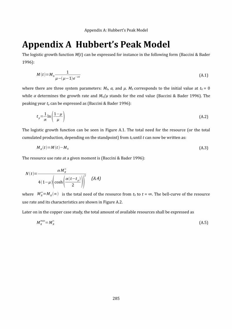
Appendix A: Hubbert’s Peak ModelAppendix A Hubbert’s Peak ModelThe logistic growth function M(t) can be expressed for instance in the following form (Baccini & Bader 1996):

M t =M 0 1−−1e−t (A.1)

where there are three system parameters: M0, α, and μ. M0 corresponds to the initial value at t0 = 0 while α determines the growth rate and M0/μ stands for the end value (Baccini & Bader 1996). The peaking year tp can be expressed as (Baccini & Bader 1996):t p=

1

ln1− (A.2)

The logistic growth function can be seen in Figure A.1. The total need for the resource (or the total cumulated production, depending on the standpoint) from t0 until t can now be written as: M R t =M t −M 0 (A.3)The resource use rate at a given moment is (Baccini & Bader 1996):

N t =M R

∞

41−cosht−t p 2 2

(A.4)

where M R∞=M R ∞ is the total need of the resource from t0 to t = ∞. The bell-curve of the resource use rate and its characteristics are shown in Figure A.2.Later on in the copper case study, the total amount of available resources shall be expressed as

M Rmax=M R

∞ (A.5)

285

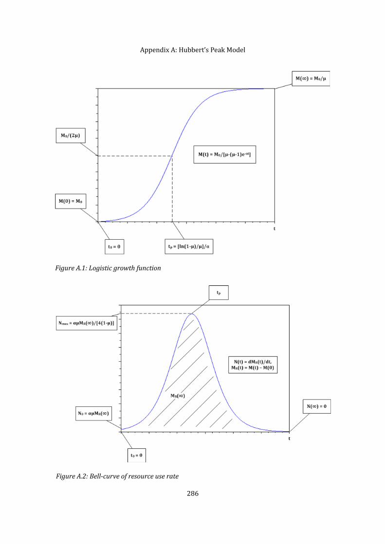
Appendix A: Hubbert’s Peak Model

286

Figure A.1: Logistic growth function

Figure A.2: Bell-curve of resource use rate

Appendix B: Case Study on CopperAppendix B Case Study on CopperCopper Metabolism in Geneva in 2000There were some minor discrepancies in the original SFA (Faist Emmenegger & Frischknecht 2003); I have chosen to use corrected values of net addition to stock (marked in yellow). Table B.1: Copper metabolism in the Canton of Geneva in 2000

The copper flows per capita are based on the previously listed copper flows divided by the Geneva population in 2000, namely 413,585 inhabitants (OCSTAT 2011c).

287

Copper Metabolism in Geneva [t]

Primary sector Input Export Recycling Incineration Input stock StockVehicles 2 1 2 0 -1 32Buildings 82 0 70 23 -11 1545Total 85 1 71 24 -12 1578

Secondary sector Input Export Recycling Incineration Input stock StockFabrication of machines and equipment 1910 1058 750 52 50 0Watchmaking 5 5 0 0 0 0Electronic/electric appliances 8 5 1,7 1,7 -0,4 0Buildings 263 0 125 42 96 20700Total 2187 1068 876 95 146 20700

Tertiary sector Input Export Recycling Incineration Input stock StockElectronic/electric appliances 58 35 11,6 11,6 -0,2 223Vehicles 83 19 34 8 22 1474Buildings 1104 0 408 136 560 34331Total 1245 54 453 156 582 36029

Households Input Export Recycling Incineration Input stock StockFurniture 21 0 13 5 3 388Electronic/electric appliances 60 36 11,9 11,9 0,2 372Packaging materials 0 0 0 0 0 0Vehicles 131 31 55 14 31 1885Buildings 690 0 236 79 375 29122Household appliances 44 0 19 19 6 580Total 946 67 335 128 415 32347

Total 4462 1190 1736 402 1131 90654

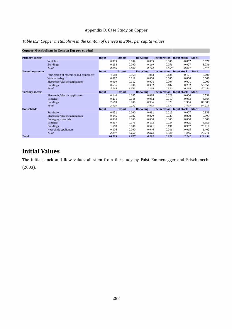
Appendix B: Case Study on CopperTable B.2: Copper metabolism in the Canton of Geneva in 2000, per capita values

Initial ValuesThe initial stock and flow values all stem from the study by Faist Emmenegger and Frischknecht (2003).

288

Copper Metabolism in Geneva [kg per capita]

Primary sector Input Export Recycling Incineration Input stock StockVehicles 0.005 0.002 0.005 0.000 -0.002 0.077Buildings 0.198 0.000 0.169 0.056 -0.027 3.736Total 0.206 0.002 0.172 0.058 -0.027 3.815

Secondary sector Input Export Recycling Incineration Input stock StockFabrication of machines and equipment 4.618 2.558 1.813 0.126 0.121 0.000Watchmaking 0.012 0.012 0.000 0.000 0.000 0.000Electronic/electric appliances 0.019 0.012 0.004 0.004 -0.001 0.000Buildings 0.636 0.000 0.302 0.102 0.232 50.050Total 5.288 2.582 2.118 0.230 0.358 50.050

Tertiary sector Input Export Recycling Incineration Input stock StockElectronic/electric appliances 0.140 0.085 0.028 0.028 0.000 0.539Vehicles 0.201 0.046 0.082 0.019 0.053 3.564Buildings 2.669 0.000 0.986 0.329 1.354 83.008Total 3.010 0.131 1.095 0.377 1.407 87.114

Households Input Export Recycling Incineration Input stock StockFurniture 0.051 0.000 0.031 0.012 0.007 0.938Electronic/electric appliances 0.145 0.087 0.029 0.029 0.000 0.899Packaging materials 0.000 0.000 0.000 0.000 0.000 0.000Vehicles 0.317 0.075 0.133 0.034 0.075 4.558Buildings 1.668 0.000 0.571 0.191 0.907 70.414Household appliances 0.106 0.000 0.046 0.046 0.015 1.402Total 2.287 0.162 0.810 0.309 1.006 78.211

Total 10.789 2.877 4.197 0.972 2.742 219.191

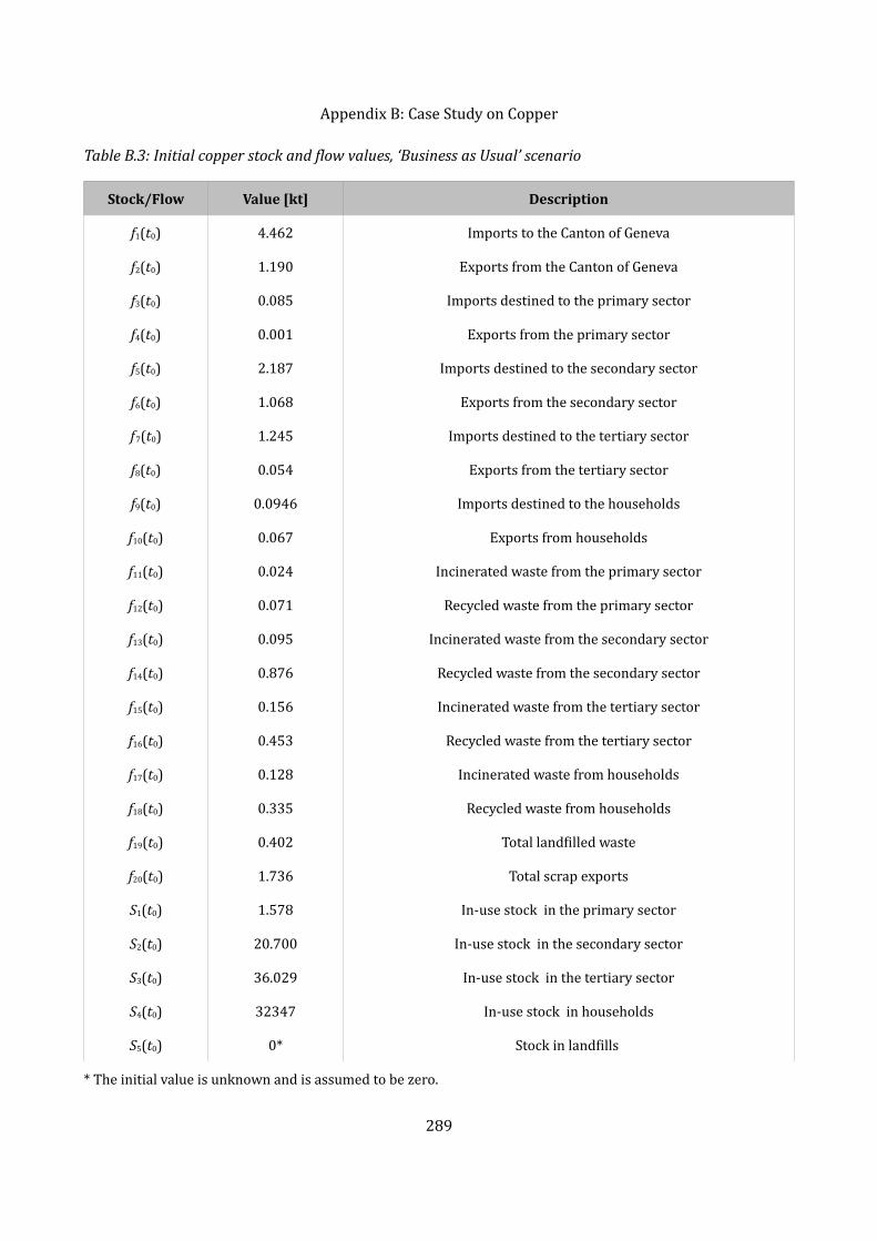
Appendix B: Case Study on CopperTable B.3: Initial copper stock and flow values, ‘Business as Usual’ scenario

Stock/Flow Value [kt] Description

f1(t0) 4.462 Imports to the Canton of Genevaf2(t0) 1.190 Exports from the Canton of Genevaf3(t0) 0.085 Imports destined to the primary sectorf4(t0) 0.001 Exports from the primary sectorf5(t0) 2.187 Imports destined to the secondary sectorf6(t0) 1.068 Exports from the secondary sectorf7(t0) 1.245 Imports destined to the tertiary sectorf8(t0) 0.054 Exports from the tertiary sectorf9(t0) 0.0946 Imports destined to the householdsf10(t0) 0.067 Exports from householdsf11(t0) 0.024 Incinerated waste from the primary sectorf12(t0) 0.071 Recycled waste from the primary sectorf13(t0) 0.095 Incinerated waste from the secondary sectorf14(t0) 0.876 Recycled waste from the secondary sectorf15(t0) 0.156 Incinerated waste from the tertiary sectorf16(t0) 0.453 Recycled waste from the tertiary sectorf17(t0) 0.128 Incinerated waste from householdsf18(t0) 0.335 Recycled waste from householdsf19(t0) 0.402 Total landfilled wastef20(t0) 1.736 Total scrap exportsS1(t0) 1.578 In-use stock in the primary sectorS2(t0) 20.700 In-use stock in the secondary sectorS3(t0) 36.029 In-use stock in the tertiary sectorS4(t0) 32347 In-use stock in householdsS5(t0) 0* Stock in landfills * The initial value is unknown and is assumed to be zero.

289

Appendix B: Case Study on CopperScenario ValuesThe data on the consumption scenarios are relative to the Geneva population in 2000. The differences compared to the ‘Business as Usual’ values are highlighted in yellow.

When t ≤ 2010, initial values fi(t0) identical to those of the ‘Business as Usual’ scenario are used in the simulations. When t ≥ 2020, the scenario-specific values presented below are employed. Between these two time points, a linear interpolation of the two values is made. ‘90% Recycling of Building Waste’ Scenario The recycled copper from buildings has increased by a factor of 0.90/0.75 compared to the year 2000 SFA. Table B.4: Copper metabolism, ‘90% Recycling of Building Waste’ scenario

290

Building Waste Recycling Attains 90 % [t]

Primary sector Input Export Recycling Incineration Input stock StockVehicles 2 1 2 0 -1 32Buildings 82 0 84 9 -11.2 1545Total 84 1 86 9 -12.2 1578

Secondary sector Input Export Recycling Incineration StockFabrication of machines and equipment 1910 1058 750 52 50 0Watchmaking 5 5 0 0 0 0Electronic/electric appliances 8 5 2 2 -0.4 0Buildings 263 0 150 17 96.2 20700Total 2186 1068 902 71 145.8 20700

Tertiary sector Input Export Recycling Incineration StockElectronic/electric appliances 58 35 12 12 -0.2 223Vehicles 83 19 34 8 22 1474Buildings 1104 0 490 54 560 34331Total 1245 54 535 74 581.8 36029

Households Input Export Recycling Incineration StockFurniture 21 0 13 5 3 388Electronic/electric appliances 60 36 12 12 0.2 372Packaging materials 0 0 0 0 0 0Vehicles 131 31 55 14 31 1885Buildings 690 0 283 32 375.2 29122Household appliances 44 0 19 19 6 580Total 946 67 382 82 415.4 32347

Total 4461 1190 1905 235 1130.8 90654

Appendix B: Case Study on CopperTable B.5: Copper stock and flow values, ‘90% Recycling of Building Waste’ scenario

Stock/Flow Value [kt] Description

f11(t1) 0.009 Incinerated waste from the primary sectorf12(t1) 0.086 Recycled waste from the primary sectorf13(t1) 0.071 Incinerated waste from the secondary sectorf14(t1) 0.902 Recycled waste from the secondary sectorf15(t1) 0.074 Incinerated waste from the tertiary sectorf16(t1) 0.535 Recycled waste from the tertiary sectorf17(t1) 0.082 Incinerated waste from householdsf18(t1) 0.382 Recycled waste from householdsf19(t1) 4.606 Total landfilled wastef20(t1) 0.569 Total scrap exports

‘Substitution in Roofing and Guttering’ Scenario The copper consumption in buildings has decreased by 41% compared to the year 2000 SFA. This represents the part of roofing and coppering in this activity in Switzerland (Faist Emmenegger & Frischknecht 2003).

291

Appendix B: Case Study on CopperTable B.6: Copper metabolism, ‘Substitution in Roofing and Guttering’ scenario

Table B.7: Copper stock and flow values, ‘Substitution in Roofing and Guttering’ scenario

Stock/Flow Value [kt] Description

f1(t0) 3.584 Imports to the Canton of Genevaf3(t0) 0.050 Imports destined for the primary sectorf5(t0) 2.078 Imports destined for the secondary sectorf7(t0) 0.792 Imports destined for the tertiary sectorf9(t0) 0.663 Imports destined for households

‘Electric Mobility’ Scenario The copper values in vehicles have been doubled compared to the year 2000 SFA.

292

Substitution of Copper in Roofing and Guttering [t]

Primary sector Input Export Recycling Incineration Input stock StockVehicles 2 1 2 0 -1 32Buildings 48 0 70 23 -44.62 1545Total 50 1 71 24 -45.62 1578

Secondary sector Input Export Recycling Incineration Input stock StockFabrication of machines and equipment 1910 1058 750 52 50 0

5 5 0 0 0 0Electronic/electric appliances 8 5 1.7 1.7 -0.4 0Buildings 155 0 125 42 -11.83 20700Total 2078 1068 876 95 37.77 20700

Tertiary sector Input Export Recycling Incineration Input stock StockElectronic/electric appliances 58 35 11.6 11.6 -0.2 223Vehicles 83 19 34 8 22 1474Buildings 651 0 408 136 107.36 34331Total 792 54 453 156 129.16 36029

Households Input Export Recycling Incineration Input stock StockFurniture 21 0 13 5 3 388Electronic/electric appliances 60 36 11.9 11.9 0.2 372Packaging materials 0 0 0 0 0 0Vehicles 131 31 55 14 31 1885Buildings 407 0 236 79 92.1 29122Household appliances 44 0 19 19 6 580Total 663 67 335 128 132.3 32347

Total 3584 1190 1736 402 253.61 90654

Watchmaking

Appendix B: Case Study on CopperTable B.8: Copper metabolism, ‘E-Mobility’ scenario

Table B.9: Copper stock and flow values, ‘E-Mobility’ scenario

Stock/Flow Value [kt] Description

f1(t0) 4.677 Imports to the Canton of Genevaf2(t0) 1.241 Exports from the Canton of Genevaf3(t0) 0.086 Imports destined for the primary sectorf4(t0) 0.002 Exports from the primary sectorf5(t0) 2.186 Imports destined for the secondary sectorf6(t0) 1.068 Exports from the secondary sectorf 7(t0) 1.328 Imports destined for the tertiary sectorf8(t0) 0.073 Exports from the tertiary sectorf9(t0) 1.077 Imports destined for householdsf10(t0) 0.098 Exports from households

‘No Primary Copper Consumption’ Scenario The initial values of the ‘No Primary Copper’ Scenario correspond to the values of the baseline scenario. 293

Increase of Copper Use in Electric Mobility [t]

Primary sector Input Export Recycling Incineration Input stock StockVehicles 4 2 2 0 0 32Buildings 82 0 70 23 -11 1545Total 86 2 71 24 -11 1578

Secondary sector Input Export Recycling Incineration Input stock StockFabrication of machines and equipment 1910 1058 750 52 50 0

5 5 0 0 0 0Electronic/electric appliances 8 5 1.7 1.7 -0.4 0Buildings 263 0 125 42 96 20700Total 2186 1068 876 95 145.6 20700

Tertiary sector Input Export Recycling Incineration Input stock StockElectronic/electric appliances 58 35 11.6 11.6 -0.2 223Vehicles 166 38 34 8 86 1474Buildings 1104 0 408 136 560 34331Total 1328 73 453 156 645.8 36029

Households Input Export Recycling Incineration Input stock StockFurniture 21 0 13 5 3 388Electronic/electric appliances 60 36 11.9 11.9 0.2 372Packaging materials 0 0 0 0 0 0Vehicles 262 62 55 14 131 1885Buildings 690 0 236 79 375 29122Household appliances 44 0 19 19 6 580Total 1077 98 335 128 515.2 32347

Total 4677 1241 1736 402 1295.6 90654

Watchmaking

Appendix B: Case Study on CopperCopper Residence TimesThe copper residence times have been calculated as a weighted average based on different copper uses in the sectors. The values from van Beers et al. (2007) have been averaged whereas this was not necessary for Spatari et al. (2005). The sectorial residence times have been calculated as weighted averages.Table B.10: Copper residence times in different economic sectors

Model DescriptionSystem VariablesFlows: f 1, f 2, f 3, f 4, f 5, f 6, f 7, f 8, f 9, f 10, f 11, f 12, f 13, f 14, f 15, f 16, f 17, f 18, f 19, f 20Stocks: S1, S2, S3, S4, S5Additions to stock: S1, S2, S3, S4, S5There are 30 unknowns (20 flows, 5 stocks and 5 changes in stock). State EquationsState equations for the system can be written as:

294

Source1 10Buildings 82 45TOTAL 84 44852 200 203 20Buildings 263 45TOTAL 1119 2623 20 Business durables64 10Buildings 1104 45TOTAL 1191 4321 10 Consumer24 10 Consumer0 10 Consumer100 10Buildings 690 4544 10 ConsumerTOTAL 879 37

Copper Residence Times [y]

Primary sector Net copper imports Residence time Source categoryVehicles Spatari et al. (2005) Motor vehiculesvan Beers et al. (2007) Building and constructionSecondary sectorFabrication of machines and equipment Spatari et al. (2005) IndustrialWatchmaking Spatari et al. (2005) IndustrialElectronic/electric appliances Spatari et al. (2005) Industrialvan Beers et al. (2007) Building and constructionTertiary sectorElectronic/electric appliances van Beers et al. (2007)Vehicles Spatari et al. (2005) Motor vehiculesvan Beers et al. (2007) Building and constructionHouseholdsFurniture Spatari et al. (2005)Electronic/electric appliances Spatari et al. (2005)Packaging materials Spatari et al. (2005)Vehicles Spatari et al. (2005) Motor vehiculesvan Beers et al. (2007) Building and constructionHousehold appliances Spatari et al. (2005)

Appendix B: Case Study on CopperS1t = f 3t − f 4t − f 11t − f 12t S2t = f 5t − f 6t − f 13t − f 14t S3t = f 7t − f 8t − f 15t − f 16t S4t = f 9t − f 10t − f 17t − f 18t S5t = f 19t There are three processes (‘Distribution’, ‘Incineration and treatment’ and ‘Recycling’) where there is no addition to stock: f 1t − f 2t = f 3t − f 4t f 5t − f 6t f 7t − f 8t f 9t − f 10t f 11t f 13t f 15 t f 17 t = f 19 t f 12t f 14t f 16t f 18 t = f 20 t In addition, it is always true thatS i t1=S i t S i t , i∈{1,2 ,3 ,4 ,5}

295

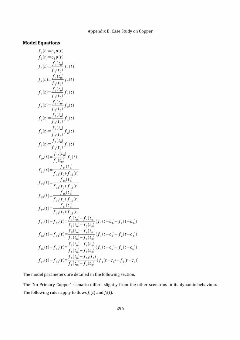
Appendix B: Case Study on CopperModel Equations

f 1t =c1 pt f 2t =c2 pt

f 3t = f 3t0f 1t0 f 1t

f 4t = f 4t0f 2t 0 f 2t

f 5t = f 5t0f 1t0 f 1t

f 6t = f 6t0f 2t 0 f 2t

f 7t = f 7t0f 1t0 f 1t

f 8t = f 8t0f 2t0 f 2t

f 9t = f 9t0f 1t0 f 1t

f 10t = f 10 t 0f 2t0 f 2t

f 11t = f 11t 0f 12t0⋅f 12 t

f 13t = f 13t0f 14t0⋅f 14 t

f 15t = f 15t 0f 16t0⋅f 16 t

f 17t = f 17t 0f 18t0⋅f 18 t

f 11t f 12t = f 3t0− f 4t0f 1t0− f 2t 0 f 1t−c3− f 2t−c3

f 13t f 14t = f 5t0− f 6t0f 1t0− f 2t0 f 1t−c4− f 2t−c 4

f 15t f 16t = f 7t0− f 8t 0f 1t0− f 2t 0 f 1t−c5− f 2t−c5

f 17t f 18t = f 9t0− f 10t 0f 1t0− f 2t 0 f 1t−c6− f 2t−c6

The model parameters are detailed in the following section.The ‘No Primary Copper’ scenario differs slightly from the other scenarios in its dynamic behaviour. The following rules apply to flows f1(t) and f2(t).296

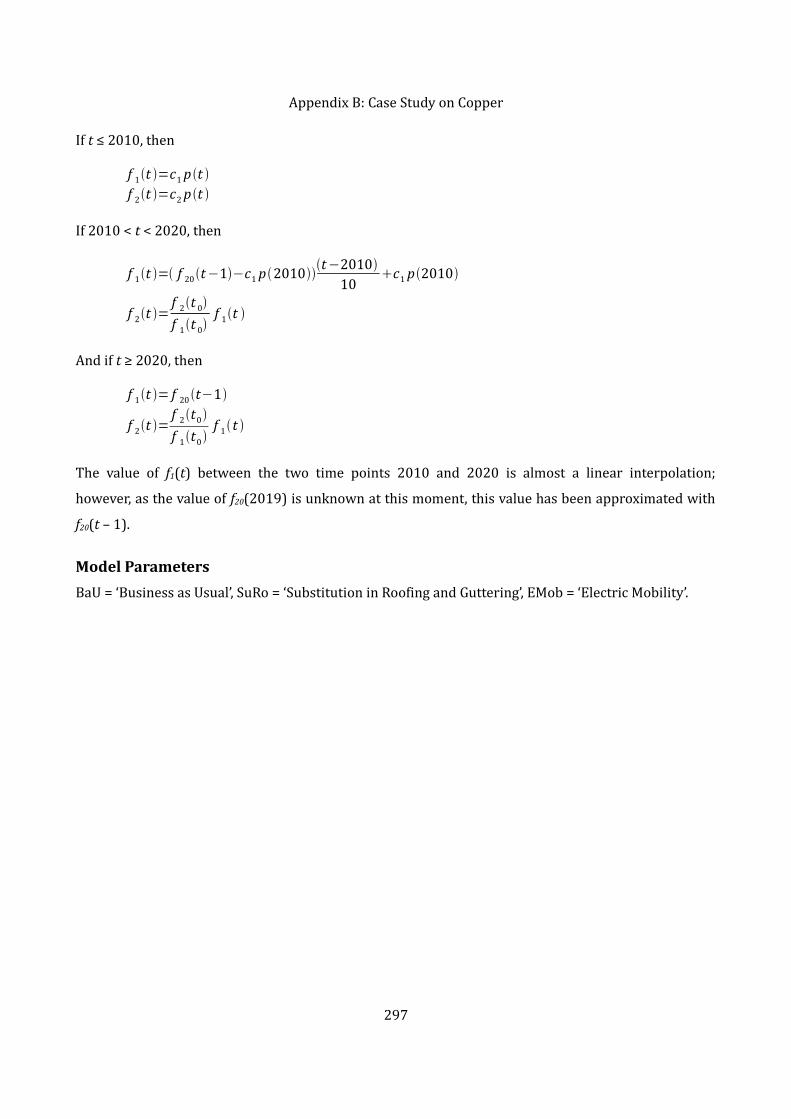
Appendix B: Case Study on CopperIf t ≤ 2010, thenf 1t =c1 pt f 2t =c2 pt If 2010 < t < 2020, thenf 1t = f 20t−1−c1 p2010t−201010 c1 p2010f 2t = f 2t 0

f 1t 0 f 1t And if t ≥ 2020, then

f 1t = f 20 t−1f 2t = f 2t0

f 1t0 f 1t The value of f1(t) between the two time points 2010 and 2020 is almost a linear interpolation; however, as the value of f20(2019) is unknown at this moment, this value has been approximated with f20(t – 1).Model ParametersBaU = ‘Business as Usual’, SuRo = ‘Substitution in Roofing and Guttering’, EMob = ‘Electric Mobility’.

297

Appendix B: Case Study on CopperTable B.11: Copper model parameters

Model Parameter

Parameter Description Constant Value if Constant

c1 The relation between copper imports and the Geneva populationYes f1(t0)/p(t0) = 10.8 kg (BaU)8.7 kg (SuRo)11.3 kg (EMob)

c2 The relation between copper exports (products) and the Geneva populationYes f2(t0)/p(t0) = 2.9 kg

c3 The copper lifespan in the primary sector Yes 44 yearsc4 The copper lifespan in the secondary sector Yes 26 yearsc5 The copper lifespan in the tertiary sector Yes 43 yearsc6 The copper lifespan in households Yes 37 years

p(t) The size of the population No -t0 The starting year of the simulation Yes 2000

The fi(t0) correspond to the initial values of the flows.Model ResultsThe results of the copper simulations are seen in the following tables.

298

Appendix B: Case Study on Copper

299BaU = ‘Business as Usual’, BuWa = ‘90% Recycling of Building Waste’, SuRo = ‘Substitution in Roofing and Guttering’, EMob = ‘Electric Mobility’, NoPC = ‘No Primary Copper Consumption’.Figure B.1: Copper net imports

Appendix B: Case Study on Copper

300BaU = ‘Business as Usual’, BuWa = ‘90% Recycling of Building Waste’, SuRo = ‘Substitution in Roofing and Guttering’, EMob = ‘Electric Mobility’, NoPC = ‘No Primary Copper Consumption’.Figure B.2: Primary and secondary copper use

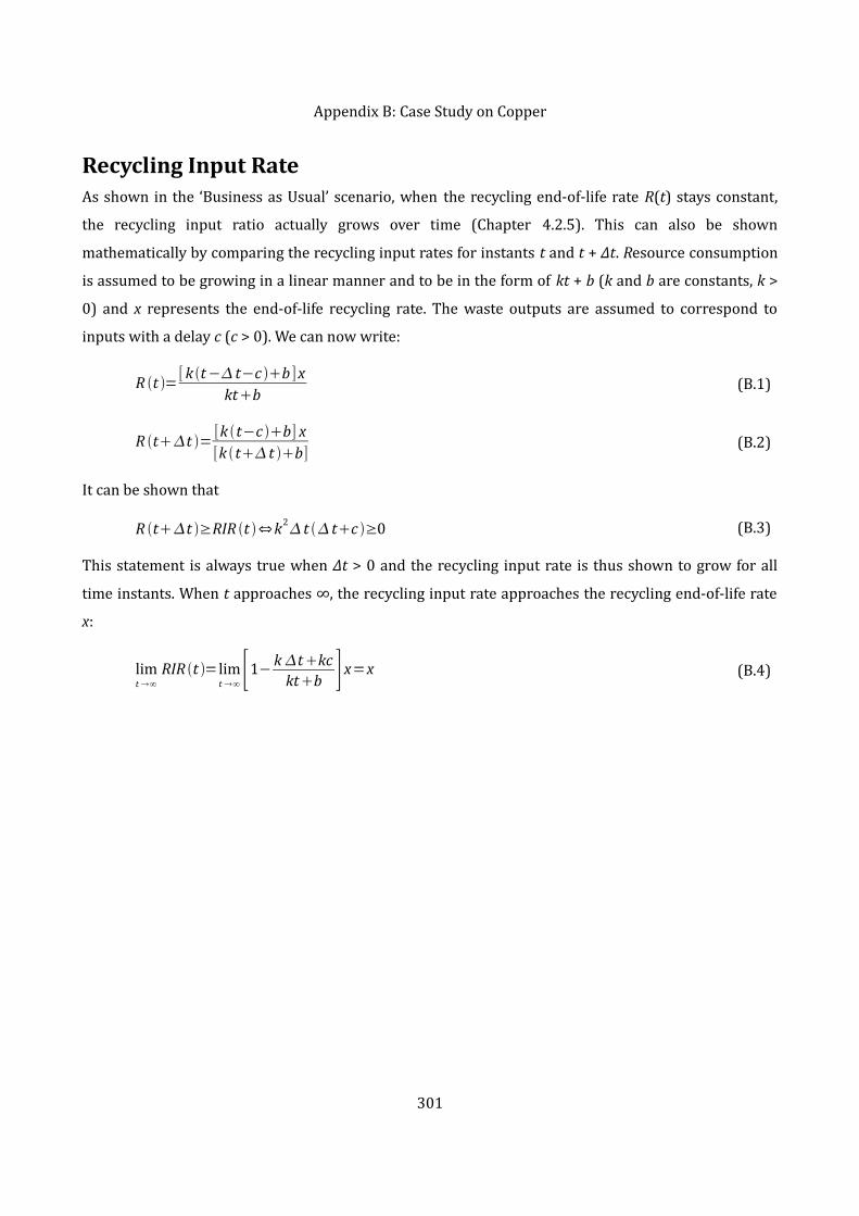
Appendix B: Case Study on CopperRecycling Input RateAs shown in the ‘Business as Usual’ scenario, when the recycling end-of-life rate R(t) stays constant, the recycling input ratio actually grows over time (Chapter 4.2.5). This can also be shown mathematically by comparing the recycling input rates for instants t and t + Δt. Resource consumption is assumed to be growing in a linear manner and to be in the form of kt + b (k and b are constants, k > 0) and x represents the end-of-life recycling rate. The waste outputs are assumed to correspond to inputs with a delay c (c > 0). We can now write:

R t =[k t− t−c b ]xktb

(B.1)R tt = [k t−c b] x

[k t t b](B.2)

It can be shown that R tt ≥RIR t ⇔k2 t tc ≥0 (B.3)This statement is always true when Δt > 0 and the recycling input rate is thus shown to grow for all time instants. When t approaches ∞, the recycling input rate approaches the recycling end-of-life rate

x:limt ∞

RIR t = limt ∞ [1− k tkc

ktb ] x=x (B.4)

301

Appendix B: Case Study on CopperSensitivity AnalysisS1 = primary sector, S2 = secondary sector, S3 = tertiary sector, HH = households.Table B.12: Sensitivity scenarios

Scenario Tested Parameter Change in Value [%]Scenario 1 Net imports per capita to S1 ±30%Scenario 2 Net imports per capita to S2 ±30%Scenario 3 Net imports per capita to S3 ±30%Scenario 4 Net imports per capita to HH ±30%Scenario 5 Copper residence time in S1 ±50%Scenario 6 Copper residence time in S2 ±50%Scenario 7 Copper residence time in S3 ±50%Scenario 8 Copper residence time in HH ±50%Scenario 9 Recycling rate in S1 ±5%Scenario 10 Recycling rate in S2 ±5%Scenario 11 Recycling rate in S3 ±5%Scenario 12 Recycling rate in HH ±5%The sensitivity parameter values have been calculated for (1) the primary copper consumption in 2080 and (2) for the cumulated primary copper consumption by comparing the maximum and minimum values. Sensitivity values greater than 10% (relative sensitivity) and 20% (100% relative sensitivity) are marked in grey. S1 = primary sector, S2 = secondary sector, S3 = tertiary sector, HH = households.

302

Appendix B: Case Study on CopperTable B.13: Synthesis of sensitivity analysis results

Net Imports per Capita Residence Time Recycling Rate

S1 S2 S3 HH S1 S2 S3 HH S1 S2 S3 HHOriginal parameter value 0.20 kg 2.7 kg 2.9 kg 2.1 kg 44 y 26 y 43 y 37 y 75% 90% 74% 72%Parameter variation 30% 30% 30% 30% 50% 50% 50% 50% 5% 5% 5% 5%

Min parameter value 0.14 kg 1.9 kg 2.0 kg 1.5 kg 22 y 13 y 22 y 19 y 71% 95% 71% 69%Max parameter value 0.26 kg 3.5 kg 3.7 kg 2.8 kg 66 y 39 y 65 y 56 y 78% 86% 78% 76%(1) Min primary copper 2080 1.79 kt 1.69 kt 1.60 kt 1.63 kt 1.80 kt 1.71 kt 1.67 kt 1.72 kt 1.80 kt 1.73 kt 1.75 kt 1.76 kt(1) Max primary copper 2080 1.82 kt 1.92 kt 2.04 kt 1.98 kt 1.82 kt 1.91 kt 1.96 kt 1.90 kt 1.81 kt 1.88 kt 1.87 kt 1.85 kt

(1) Absolute sensitivity 0.28 0.14 0.28 0.27 0.00048 0.0076 0.0068 0.0048 -0.0011 -0.016 -0.016 -0.012(1) Relative sensitivity 0.15 0.073 0.13 0.14 0.00026 0.0040 0.0035 0.0025 -0.00061 -0.0094 -0.0090 -0.0068(1) 100% absolute sensitivity 0.072 0.49 1.0 0.75 0.032 0.30 0.44 0.27 -0.087 -1.5 -1.2 -0.92

303

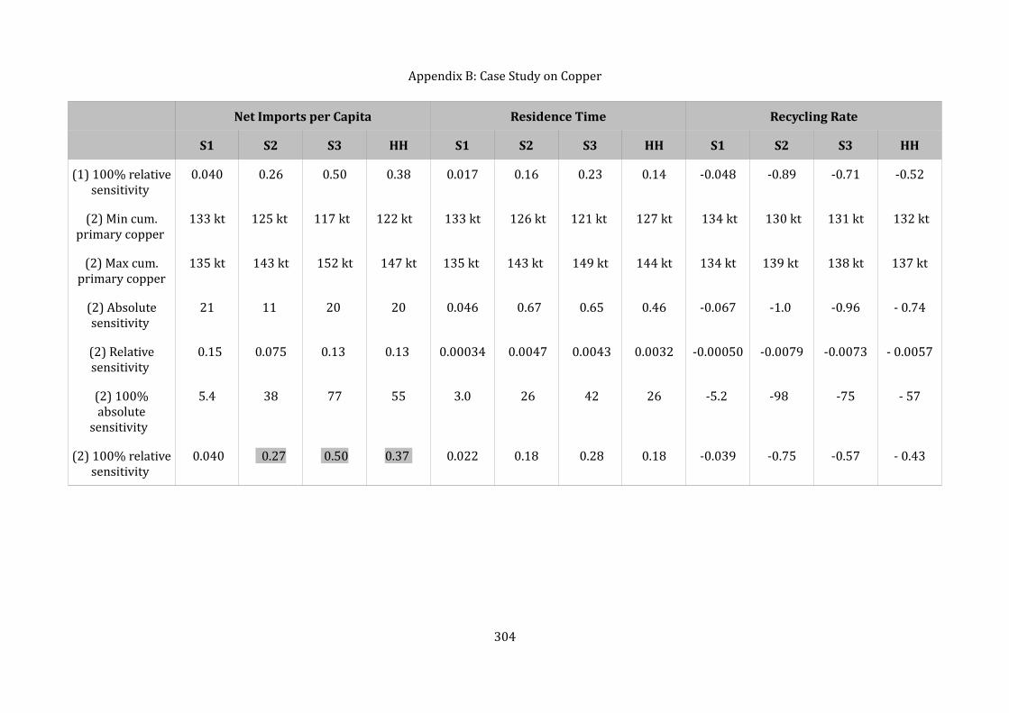
Appendix B: Case Study on CopperNet Imports per Capita Residence Time Recycling Rate

S1 S2 S3 HH S1 S2 S3 HH S1 S2 S3 HH(1) 100% relative sensitivity 0.040 0.26 0.50 0.38 0.017 0.16 0.23 0.14 -0.048 -0.89 -0.71 -0.52(2) Min cum. primary copper 133 kt 125 kt 117 kt 122 kt 133 kt 126 kt 121 kt 127 kt 134 kt 130 kt 131 kt 132 kt(2) Max cum. primary copper 135 kt 143 kt 152 kt 147 kt 135 kt 143 kt 149 kt 144 kt 134 kt 139 kt 138 kt 137 kt(2) Absolute sensitivity 21 11 20 20 0.046 0.67 0.65 0.46 -0.067 -1.0 -0.96 - 0.74(2) Relative sensitivity 0.15 0.075 0.13 0.13 0.00034 0.0047 0.0043 0.0032 -0.00050 -0.0079 -0.0073 - 0.0057(2) 100% absolute sensitivity 5.4 38 77 55 3.0 26 42 26 -5.2 -98 -75 - 57

(2) 100% relative sensitivity 0.040 0.27 0.50 0.37 0.022 0.18 0.28 0.18 -0.039 -0.75 -0.57 - 0.43

304

Appendix B: Case Study on Copper

305

Figure B.3: Sensitivity to sectorial net imports per capita, scenarios 1–4, results for net imports

Appendix B: Case Study on Copper

306

Figure B.4: Sensitivity to residence time, scenarios 5–8, results for net imports

Appendix B: Case Study on Copper

307

Figure B.5: Sensitivity to recycling rate, scenarios 9–12, results for net imports

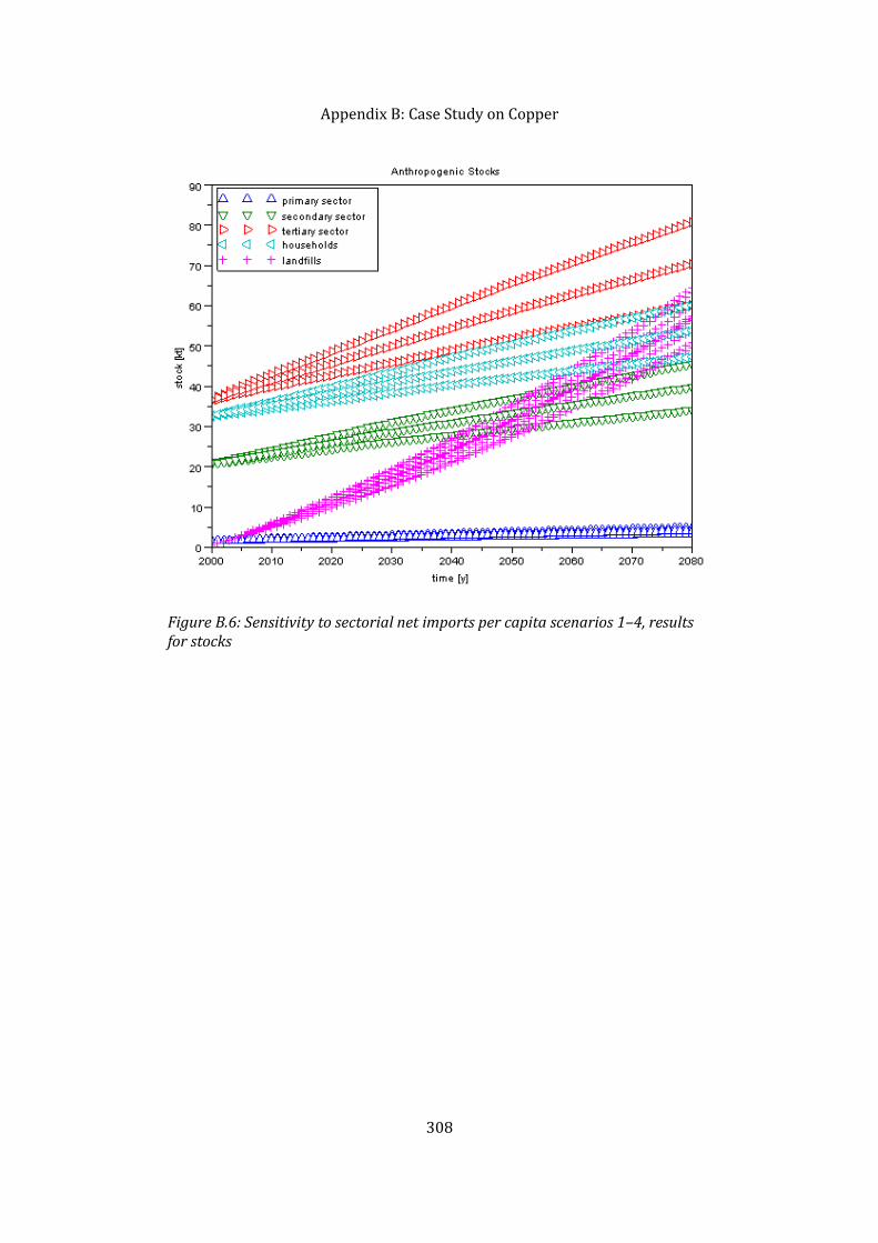
Appendix B: Case Study on Copper

308

Figure B.6: Sensitivity to sectorial net imports per capita scenarios 1–4, results for stocks

Appendix B: Case Study on Copper

309

Figure B.7: Sensitivity to residence time, scenarios 5–8, results for stocks

Appendix B: Case Study on Copper

Historical Copper ProductionThe cumulated world mine production of copper before the industrial revolution is based on estimations of Hong et al. (1996). In this estimation, the data for the Roman production, the Chinese production till 750 and the mid- and late medieval world production values were taken into account. The cumulated world mine production during the industrial revolution (1750–1900) has been calculated based on production and growth rate data from Radetzki (2009).

310

Figure B.8: Sensitivity to recycling rate, scenarios 9–12, results for stocks

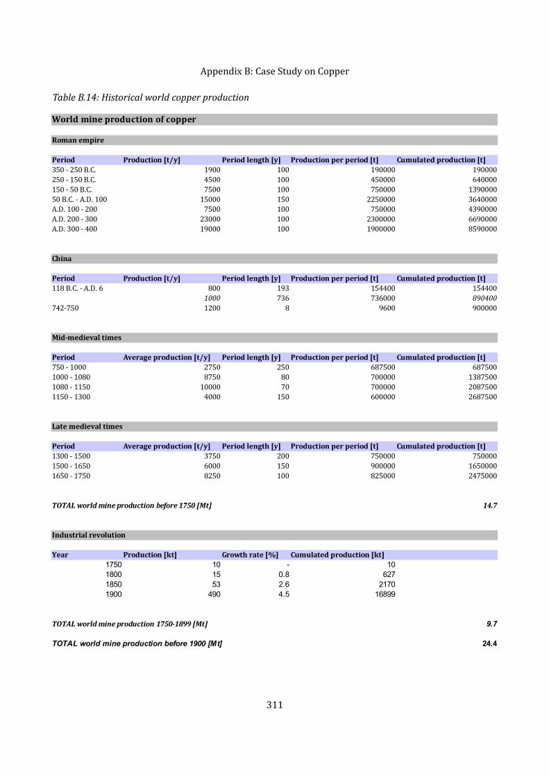
Appendix B: Case Study on CopperTable B.14: Historical world copper production

311

Roman empire

Production [t/y]350 - 250 B.C. 1900 100 190000 190000250 - 150 B.C. 4500 100 450000 640000150 - 50 B.C. 7500 100 750000 139000050 B.C. - A.D. 100 15000 150 2250000 3640000A.D. 100 - 200 7500 100 750000 4390000A.D. 200 - 300 23000 100 2300000 6690000A.D. 300 - 400 19000 100 1900000 8590000China

Production [t/y]118 B.C. - A.D. 6 800 193 154400 1544001000 736 736000 890400742-750 1200 8 9600 900000

750 - 1000 2750 250 687500 6875001000 - 1080 8750 80 700000 13875001080 - 1150 10000 70 700000 20875001150 - 1300 4000 150 600000 2687500

1300 - 1500 3750 200 750000 7500001500 - 1650 6000 150 900000 16500001650 - 1750 8250 100 825000 247500014.7

Production [kt]1750 10 - 101800 15 0.8 6271850 53 2.6 21701900 490 4.5 16899

9.7

TOTAL world mine production before 1900 [Mt] 24.4

World mine production of copper

Period Period length [y] Production per period [t] Cumulated production [t]

Period Period length [y] Production per period [t] Cumulated production [t]

Mid-medieval times

Period Average production [t/y] Period length [y] Production per period [t] Cumulated production [t]

Late medieval times

Period Average production [t/y] Period length [y] Production per period [t] Cumulated production [t]

TOTAL world mine production before 1750 [Mt]

Industrial revolution

Year Growth rate [%] Cumulated production [kt]

TOTAL world mine production 1750-1899 [Mt]

Appendix B: Case Study on CopperFuture World Copper ProductionThe mathematical formula of the logistic growth function and its derivative can be seen in Appendix A. The future world copper production has been estimated by fitting a bell-curve (derivative of the logistic curve) to the historical data on annual copper production values. Two different estimates for the amount of total available resources were used and two estimated copper production curves are thus obtained. Table B.15: Estimated world copper production curves

Total available resources [Gt] Estimated peak year Estimated α Estimated μ1.6 2026 0.042 0.00524.3 2066 0.033 0.0038

312

Appendix C: Case Study on PhosphorusAppendix C Case Study on PhosphorusNormalized ScenariosThe following tables present the results of the normalized Swiss scenarios. Cells marked in yellow mark calculations where various interactions (imports, exports, or local production) have been taken into account. Slightly darkened lines denote internal system flows that have been taken into account in order to split the agricultural processes between primary and secondary sectors. Darkened lines in the recycling scenarios denote differences with the ‘Business as Usual’ scenario. The slight material accumulations in ‘Chemical industry’ and ‘Households & trade’ are assumed to be due to rounding errors.

313

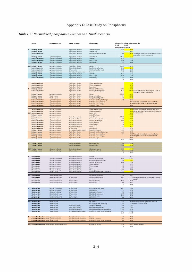
Appendix C: Case Study on PhosphorusTable C.1: Normalized phosphorus ‘Business as Usual’ scenario

314

IN 5615 0.0033 0.03688 200.48Agriculture plants 29572 31.273114 2.772766 2.4665 0.06OUT Agriculture plants 29385 26.113488 202.973015 2.6820 0.023114 2.772766 2.4665 0.060 0.00Agriculture plants 4.10Agriculture plants 8.90Agriculture plants 6.23IN Agriculture plants 5886 917.78Agriculture plants 2447 190.66Agriculture plants 29385 26.11Agriculture plants 594 32.82Agriculture plants 498 27.67Agriculture plants Agriculture plants 1660 45.53Agriculture plants Agriculture plants 0.03Agriculture plants Agriculture plants 0.29Agriculture plants Agriculture plants 0.00Agriculture plants 0.00Agriculture plants 0.00OUT Agriculture plants 0.00Agriculture plants 779.77Agriculture plants 29572 31.27Agriculture plants 180 12.03Agriculture plants 4016 233.70Agriculture plants 71 4.13Agriculture plants 158 9.19Agriculture plants 107 6.23Agriculture plants 91 2.50Agriculture plants 1071 29.37Agriculture plants Agriculture plants 1660 45.53Agriculture plants Agriculture plants 334 0.03Agriculture plants Agriculture plants 0.29Agriculture plants Agriculture plants 0.003544 106.09IN 360 12.241456 74.44OUT 1031 59.99786 26.72-1 -0.03IN 23 0.123488 202.97Agriculture plants 180 12.03Agriculture plants 4016 233.70Agriculture plants 71 4.13Agriculture plants 158 9.19Agriculture plants 107 6.231031 59.99592 32.90OUT 69 4.026097 353.572503 145.65998 58.07-1 -0.06IN 3015 2.68Agriculture plants 91 2.50786 26.726097 353.572503 145.65998 58.07OUT 185 10.441505 1.34Agriculture plants 594 32.82Agriculture plants 498 27.67592 32.901069 59.069047 424.97IN Agriculture plants 20 0.02Agriculture plants 1071 29.371069 59.06OUT 2160 88.450 0.00

Sector Output process Input process Flow name Flow value [t/a]

Flow value [t/a]

Remarks

SwitzerlandGenevaPrimary sector Agriculture animals Animal feed imp.Primary sector Agriculture animals Animals imp.Secondary sector Agriculture animals Food of animal origin imp. To simplify the situation, all butcher waste is assumed to come from importsPrimary sector Agriculture animals Animal feedSecondary sector Agriculture animals Agriculture animals AnimalsSecondary sector Agriculture animals Agriculture animals Milk & EggsPrimary sector Agriculture animals Agriculture animals Fodder soupPrimary sector Agriculture animals ManureSecondary sector Agriculture animals Households & trade Food of animal originSecondary sector Agriculture animals Waste sector Offal and butcher wastePrimary sector Agriculture animals Ground and surface waters ExcretaPrimary sector Agriculture animals Agriculture animals AnimalsPrimary sector Agriculture animals Agriculture animals Milk & EggsSecondary sector Agriculture animals Agriculture animals Fodder soupSecondary sector Wood products imp.Secondary sector Wood energy imp.Secondary sector Paper imp.Primary sector Mineral fertilisers imp.Secondary sector Food of plant origin imp. To simplify the situation, all plant waste is assumed to come from importsPrimary sector Agriculture animals ManurePrimary sector Waste sector Sludge as fertiliserPrimary sector Waste sector Compost and digestateSecondary sector Domestic food of plant originSecondary sector Domestic wood products Timber is diveded into wood products, energy and wood for pulp productionSecondary sector Domestic wood energy Secondary sector Domestic paperSecondary sector Wood products exp. Imports are divided into wood products, energy and paper in the same percentages as in consumptionSecondary sector Wood energy exp.Secondary sector Paper exp.Primary sector Animal feed exp.Primary sector Agriculture animals Animal feedPrimary sector Households & trade Garden mineral fertilisersSecondary sector Households & trade Food of plant originSecondary sector Households & trade Wood productsSecondary sector Households & trade Wood energySecondary sector Households & trade PaperSecondary sector Waste sector Plant wastePrimary sector Ground and surface waters Run-off & erosionPrimary sector Domestic food of plant originPrimary sector Domestic wood products Timber is diveded into wood products, energy and wood for pulp productionPrimary sector Domestic wood energy Primary sector Domestic paperTertiary sector Chemical industry Chemicals imp.Tertiary sector Chemical industry Products imp.Tertiary sector Chemical industry Households & trade Cleaning productsTertiary sector Chemical industry Waste sector Industrial effluentsHouseholds Households & trade RainfallHouseholds Agriculture animals Households & trade Food of animal originHouseholds Households & trade Garden mineral fertilisersHouseholds Households & trade Food of plant originHouseholds Households & trade Wood productsHouseholds Households & trade Wood energyHouseholds Households & trade PaperHouseholds Chemical industry Households & trade Cleaning productsHouseholds Waste sector Households & trade Compost and digestate for gardensHouseholds Households & trade Recovered paper exp.Households Households & trade Waste sector Municipal wastewater Calculated based on the population and the rainfallHouseholds Households & trade Waste sector Municipal wasteHouseholds Households & trade Waste sector Green wasteWaste sector Agriculture animals Waste sector Offal and butcher wasteWaste sector Waste sector Plant wasteWaste sector Chemical industry Waste sector Industrial effluentsWaste sector Households & trade Waste sector Municipal wastewaterWaste sector Households & trade Waste sector Municipal wasteWaste sector Households & trade Waste sector Green wasteWaste sector Waste sector Fly ash exp. Calculated assuming that the ratios of outputs stay the sameWaste sector Waste sector Offal and butcher waste exp.Waste sector Waste sector Sludge as fertilizerWaste sector Waste sector Compost and digestateWaste sector Waste sector Households & trade Compost and digestate for gardensWaste sector Waste sector Ground and surface waters Outflow to waste water treatmentGround and surface waters Ground and surface waters ExcretaGround and surface waters Ground and surface waters Run-off & erosionGround and surface watersWaste sector Ground and surface waters Outflow to waste water treatmentGround and surface watersGround and surface waters Outflow to abroad Sum of the inputs

Appendix C: Case Study on PhosphorusTable C.2: Normalized phosphorus scenario ‘Meat and Bone Meal as Fertilizer’

315

5615 0.0033 0.03688 200.48Agriculture plants 29572 31.273114 2.772766 2.4665 0.06Agriculture plants 29385 26.113488 202.973015 2.6820 0.023114 2.772766 2.4665 0.060,00 0.00Agriculture plants 4.10Agriculture plants 8.90Agriculture plants 6.23Agriculture plants 4680 916.70Agriculture plants 2447 190.66Agriculture plants 29385 26.11Agriculture plants 594 32.82Agriculture plants 498 27.67Agriculture plants 3172 2.68Agriculture plants Agriculture plants 1660 45.53Agriculture plants Agriculture plants 0.03Agriculture plants Agriculture plants 0.29Agriculture plants Agriculture plants 0.00Agriculture plants 0.00Agriculture plants 0.00Agriculture plants 0.00Agriculture plants 779.77Agriculture plants 29572 31.27Agriculture plants 180 12.03Agriculture plants 4016 233.70Agriculture plants 71 4.13Agriculture plants 158 9.19Agriculture plants 107 6.23Agriculture plants 91 2.50Agriculture plants 1071 29.37Agriculture plants Agriculture plants 1660 45.53Agriculture plants Agriculture plants 334 0.03Agriculture plants Agriculture plants 0.29Agriculture plants Agriculture plants 0.002338,00 107.70360 12.241456 74.441031 59.99786 26.72-1,00 -0.0323 0.123488 202.97Agriculture plants 180 12.03Agriculture plants 4016 233.70Agriculture plants 71 4.13Agriculture plants 158 9.19Agriculture plants 107 6.231031 59.99592 32.9069 4.026097 353.572503 145.65998 58.07-1 -0.063015 2.68Agriculture plants 91 2.50786 26.726097 353.572503 145.65998 58.07185 10.440 0.00Agriculture plants 3015 2.68Agriculture plants 594 32.82Agriculture plants 498 27.67592 32.901069 59.067537 423.63Agriculture plants 20 0.02Agriculture plants 1071 29.371069 59.062160 88.450 0.00

Sector Output process Input process Flow name Flow value [t/a]

Flow value [t/a]

Remarks

SwitzerlandGenevaPrimary sector Agriculture animals Animal feed imp.Primary sector Agriculture animals Animals imp.Secondary sector Agriculture animals Food of animal origin imp. To simplify the situation, all butcher waste is assumed to come from importsPrimary sector Agriculture animals Animal feedSecondary sector Agriculture animals Agriculture animals AnimalsSecondary sector Agriculture animals Agriculture animals Milk & EggsPrimary sector Agriculture animals Agriculture animals Fodder soupPrimary sector Agriculture animals ManureSecondary sector Agriculture animals Households & trade Food of animal originSecondary sector Agriculture animals Waste sector Offal and butcher wastePrimary sector Agriculture animals Ground and surface waters ExcretaPrimary sector Agriculture animals Agriculture animals AnimalsPrimary sector Agriculture animals Agriculture animals Milk & EggsSecondary sector Agriculture animals Agriculture animals Fodder soupSecondary sector Wood products imp.Secondary sector Wood energy imp.Secondary sector Paper imp.Primary sector Mineral fertilisers imp. Calculated based on the BaU valueSecondary sector Food of plant origin imp. To simplify the situation, all plant waste is assumed to come from importsPrimary sector Agriculture animals ManurePrimary sector Waste sector Sludge as fertiliserPrimary sector Waste sector Compost and digestatePrimary sector Waste sector Meat and bone meal as fertiliserSecondary sector Domestic food of plant originSecondary sector Domestic wood products Timber is diveded into wood products, energy and wood for pulp productionSecondary sector Domestic wood energy Secondary sector Domestic paperSecondary sector Wood products exp. Imports are divided into wood products, energy and paper in the same percentages as in consumptionSecondary sector Wood energy exp.Secondary sector Paper exp.Primary sector Animal feed exp.Primary sector Agriculture animals Animal feedPrimary sector Households & trade Garden mineral fertilisersSecondary sector Households & trade Food of plant originSecondary sector Households & trade Wood productsSecondary sector Households & trade Wood energySecondary sector Households & trade PaperSecondary sector Waste sector Plant wastePrimary sector Ground and surface waters Run-off & erosionPrimary sector Domestic food of plant originPrimary sector Domestic wood products Timber is diveded into wood products, energy and wood for pulp productionPrimary sector Domestic wood energy Primary sector Domestic paperTertiary sector Chemical industry Chemicals imp.Tertiary sector Chemical industry Products imp.Tertiary sector Chemical industry Households & trade Cleaning productsTertiary sector Chemical industry Waste sector Industrial effluentsHouseholds Households & trade RainfallHouseholds Agriculture animals Households & trade Food of animal originHouseholds Households & trade Garden mineral fertilisersHouseholds Households & trade Food of plant originHouseholds Households & trade Wood productsHouseholds Households & trade Wood energyHouseholds Households & trade PaperHouseholds Chemical industry Households & trade Cleaning productsHouseholds Waste sector Households & trade Compost and digestate for gardensHouseholds Households & trade Recovered paper (exp.)Households Households & trade Waste sector Municipal wastewater Calculated based on the population and the rainfallHouseholds Households & trade Waste sector Municipal wasteHouseholds Households & trade Waste sector Green wasteWaste sector Agriculture animals Waste sector Offal and butcher wasteWaste sector Waste sector Plant wasteWaste sector Chemical industry Waste sector Industrial effluentsWaste sector Households & trade Waste sector Municipal wastewaterWaste sector Households & trade Waste sector Municipal wasteWaste sector Households & trade Waste sector Green wasteWaste sector Waste sector Fly ash exp. Calculated assuming that the ratios of outputs stay the sameWaste sector Waste sector Offal and butcher waste exp.Waste sector Waste sector Meat and bone meal as fertiliserWaste sector Waste sector Sludge as fertilizerWaste sector Waste sector Compost and digestateWaste sector Waste sector Households & trade Compost and digestate for gardensWaste sector Waste sector Ground and surface waters Outflow to waste water treatmentGround and surface waters Ground and surface waters ExcretaGround and surface waters Ground and surface waters Run-off & erosionGround and surface watersWaste sector Ground and surface waters Outflow to waste water treatmentGround and surface watersGround and surface waters Outflow to abroad Sum of the inputs

Appendix C: Case Study on PhosphorusTable C.3: Normalized phosphorus scenario ‘Sewage Sludge as Fertilizer’

316

IN 5615 0.0033 0.03688 200.48Agriculture plants 29572 31.273114 2.772766 2.4665 0.06OUT Agriculture plants 29385 26.113488 202.973015 2.6820 0.023114 2.772766 2.4665 0.060,00 0.00IN Agriculture plants 4498 807.60Agriculture plants 2447 190.66Agriculture plants 29385 26.11Agriculture plants 0 0.00Agriculture plants 5092 281.34Agriculture plants 498 27.67Agriculture plants Agriculture plants 1660 45.53Agriculture plants Agriculture plants 0.03Agriculture plants Agriculture plants 0.29Agriculture plants Agriculture plants 0.00Agriculture plants 0.00Agriculture plants 0.00OUT Agriculture plants 0.00Agriculture plants 779.77Agriculture plants 29572 31.27Agriculture plants 180 12.03Agriculture plants 4016 233.70Agriculture plants 71 4.13Agriculture plants 158 9.19Agriculture plants 107 6.23Agriculture plants 91 2.50Agriculture plants 1071 29.37Agriculture plants Agriculture plants 1660 45.53Agriculture plants Agriculture plants 334 0.03Agriculture plants Agriculture plants 0.29Agriculture plants Agriculture plants 0.006654,00 244.43IN 360 12.241456 74.44OUT 1031 59.99786 26.72-1,00 -0.03IN 23 0.123488 202.97Agriculture plants 180 12.03Agriculture plants 4016 233.70Agriculture plants 71 4.13Agriculture plants 158 9.19Agriculture plants 107 6.231031 59.99592 32.90OUT 69 4.026097 353.572503 145.65998 58.07-1 -0.06IN 3015 2.68Agriculture plants 91 2.50786 26.726097 353.572503 145.65998 58.07OUT 210 11.851505 1.34Agriculture plants 0 0.00Agriculture plants 5092 281.34Agriculture plants 498 27.67592 32.901069 59.064524 175.04IN Agriculture plants 20 0.02Agriculture plants 1071 29.371069 59.06OUT 2160 88.450 0.00

Sector Output process Input process Flow name Flow value [t/a]

Flow value [t/a]

Remarks

SwitzerlandGenevaPrimary sector Agriculture animals Animal feed imp.Primary sector Agriculture animals Animals imp.Secondary sector Agriculture animals Food of animal origin imp. To simplify the situation, all butcher waste is assumed to come from importsPrimary sector Agriculture animals Animal feedSecondary sector Agriculture animals Agriculture animals AnimalsSecondary sector Agriculture animals Agriculture animals Milk & EggsPrimary sector Agriculture animals Agriculture animals Fodder soupPrimary sector Agriculture animals ManureSecondary sector Agriculture animals Households & trade Food of animal originSecondary sector Agriculture animals Waste sector Offal and butcher wastePrimary sector Agriculture animals Ground and surface waters ExcretaPrimary sector Agriculture animals Agriculture animals AnimalsPrimary sector Agriculture animals Agriculture animals Milk & EggsSecondary sector Agriculture animals Agriculture animals Fodder soupPrimary sector Mineral fertilisers imp. Calculated based on the BaU valueSecondary sector Food of plant origin imp. To simplify the situation, all plant waste is assumed to come from importsPrimary sector Agriculture animals ManurePrimary sector Waste sector Sludge as fertiliserPrimary sector Waste sector Sludge ash as fertiliserPrimary sector Waste sector Compost and digestateSecondary sector Domestic food of plant originSecondary sector Domestic wood products Timber is diveded into wood products, energy and wood for pulp productionSecondary sector Domestic wood energy Secondary sector Domestic paperSecondary sector Wood products exp. Imports are divided into wood products, energy and paper in the same percentages as in consumptionSecondary sector Wood energy exp.Secondary sector Paper exp.Primary sector Animal feed exp.Primary sector Agriculture animals Animal feedPrimary sector Households & trade Garden mineral fertilisersSecondary sector Households & trade Food of plant originSecondary sector Households & trade Wood productsSecondary sector Households & trade Wood energySecondary sector Households & trade PaperSecondary sector Waste sector Plant wastePrimary sector Ground and surface waters Run-off & erosionPrimary sector Domestic food of plant originPrimary sector Domestic wood products Timber is diveded into wood products, energy and wood for pulp productionPrimary sector Domestic wood energy Primary sector Domestic paperTertiary sector Chemical industry Chemicals imp.Tertiary sector Chemical industry Products imp.Tertiary sector Chemical industry Households & trade Cleaning productsTertiary sector Chemical industry Waste sector Industrial effluentsHouseholds Households & trade RainfallHouseholds Agriculture animals Households & trade Food of animal originHouseholds Households & trade Garden mineral fertilisersHouseholds Households & trade Food of plant originHouseholds Households & trade Wood productsHouseholds Households & trade Wood energyHouseholds Households & trade PaperHouseholds Chemical industry Households & trade Cleaning productsHouseholds Waste sector Households & trade Compost and digestate for gardensHouseholds Households & trade Recovered paper (exp.)Households Households & trade Waste sector Municipal wastewater Calculated based on the population and the rainfallHouseholds Households & trade Waste sector Municipal wasteHouseholds Households & trade Waste sector Green wasteWaste sector Agriculture animals Waste sector Offal and butcher wasteWaste sector Waste sector Plant wasteWaste sector Chemical industry Waste sector Industrial effluentsWaste sector Households & trade Waste sector Municipal wastewaterWaste sector Households & trade Waste sector Municipal wasteWaste sector Households & trade Waste sector Green wasteWaste sector Waste sector Fly ash exp. Calculated assuming that the ratios of outputs stay the sameWaste sector Waste sector Offal and butcher waste exp.Waste sector Waste sector Sludge as fertiliserWaste sector Waste sector Sludge ash as fertiliserWaste sector Waste sector Compost and digestateWaste sector Waste sector Households & trade Compost and digestate for gardensWaste sector Waste sector Ground and surface waters Outflow to waste water treatmentGround and surface waters Ground and surface waters ExcretaGround and surface waters Ground and surface waters Run-off & erosionGround and surface watersWaste sector Ground and surface waters Outflow to waste water treatmentGround and surface watersGround and surface waters Outflow to abroad Sum of the inputs

Appendix C: Case Study on PhosphorusTable C.4: Normalized phosphorus scenario ‘Recycling of Green Waste’

317

IN 5615 0.0033 0.03688 200.48Agriculture plants 29572 31.273114 2.772766 2.4665 0.06OUT Agriculture plants 29385 26.113488 202.973015 2.6820 0.023114 2.772766 2.4665 0.060,00 0.00Agriculture plants 4.10Agriculture plants 8.90Agriculture plants 6.23IN Agriculture plants 5444 889.61Agriculture plants 2447 190.66Agriculture plants 29385 26.11Agriculture plants 594 32.82Agriculture plants 944 54.53Agriculture plants Agriculture plants 1660 45.53Agriculture plants Agriculture plants 0.03Agriculture plants Agriculture plants 0.29Agriculture plants Agriculture plants 0.00Agriculture plants 0.00Agriculture plants 0.00OUT Agriculture plants 0.00Agriculture plants 779.77Agriculture plants 29572 31.27Agriculture plants 180 10.72Agriculture plants 4016 233.70Agriculture plants 71 4.13Agriculture plants 158 9.19Agriculture plants 107 6.23Agriculture plants 91 2.50Agriculture plants 1071 29.37Agriculture plants Agriculture plants 1660 45.53Agriculture plants Agriculture plants 334 0.03Agriculture plants Agriculture plants 0.29Agriculture plants Agriculture plants 0.003548,00 106.09IN 360 12.241456 74.44OUT 1031 59.99786 26.72-1,00 -0.03IN 23 0.123488 202.97Agriculture plants 180 10.72Agriculture plants 4016 233.70Agriculture plants 71 4.13Agriculture plants 158 9.19Agriculture plants 107 6.231031 59.99592 34.20OUT 69 4.026097 353.571976 114.991482 86.2442 2.44IN 3015 2.68Agriculture plants 91 2.50786 26.726097 353.571976 114.991482 86.24OUT 185 9.551505 1.34Agriculture plants 594 32.82Agriculture plants 944 54.53592 34.201069 59.068558 395.19IN Agriculture plants 20 0.02Agriculture plants 1071 29.371069 59.06OUT 2160 88.450 0.00

Sector Output process Input process Flow name Flow value [t/a]

Flow value [t/a]

Remarks

SwitzerlandGenevaPrimary sector Agriculture animals Animal feed imp.Primary sector Agriculture animals Animals imp.Secondary sector Agriculture animals Food of animal origin imp. To simplify the situation, all butcher waste is assumed to come from importsPrimary sector Agriculture animals Animal feedSecondary sector Agriculture animals Agriculture animals AnimalsSecondary sector Agriculture animals Agriculture animals Milk & EggsPrimary sector Agriculture animals Agriculture animals Fodder soupPrimary sector Agriculture animals ManureSecondary sector Agriculture animals Households & trade Food of animal originSecondary sector Agriculture animals Waste sector Offal and butcher wastePrimary sector Agriculture animals Ground and surface waters ExcretaPrimary sector Agriculture animals Agriculture animals AnimalsPrimary sector Agriculture animals Agriculture animals Milk & EggsSecondary sector Agriculture animals Agriculture animals Fodder soupSecondary sector Wood products imp.Secondary sector Wood energy imp.Secondary sector Paper imp.Primary sector Mineral fertilisers imp. Calculated based on the BaU valueSecondary sector Food of plant origin imp. To simplify the situation, all plant waste is assumed to come from importsPrimary sector Agriculture animals ManurePrimary sector Waste sector Sludge as fertiliserPrimary sector Waste sector Compost and digestateSecondary sector Domestic food of plant originSecondary sector Domestic wood products Timber is diveded into wood products, energy and wood for pulp productionSecondary sector Domestic wood energy Secondary sector Domestic paperSecondary sector Wood products exp. Imports are divided into wood products, energy and paper in the same percentages as in consumptionSecondary sector Wood energy exp.Secondary sector Paper exp.Primary sector Animal feed exp.Primary sector Agriculture animals Animal feedPrimary sector Households & trade Garden mineral fertilisersSecondary sector Households & trade Food of plant originSecondary sector Households & trade Wood productsSecondary sector Households & trade Wood energySecondary sector Households & trade PaperSecondary sector Waste sector Plant wastePrimary sector Ground and surface waters Run-off & erosionPrimary sector Domestic food of plant originPrimary sector Domestic wood products Timber is diveded into wood products, energy and wood for pulp productionPrimary sector Domestic wood energy Primary sector Domestic paperTertiary sector Chemical industry Chemicals imp.Tertiary sector Chemical industry Products imp.Tertiary sector Chemical industry Households & trade Cleaning productsTertiary sector Chemical industry Waste sector Industrial effluentsHouseholds Households & trade RainfallHouseholds Agriculture animals Households & trade Food of animal originHouseholds Households & trade Garden mineral fertilisersHouseholds Households & trade Food of plant originHouseholds Households & trade Wood productsHouseholds Households & trade Wood energyHouseholds Households & trade PaperHouseholds Chemical industry Households & trade Cleaning productsHouseholds Waste sector Households & trade Compost and digestate for gardensHouseholds Households & trade Recovered paper (exp.)Households Households & trade Waste sector Municipal wastewater Calculated based on the population and the rainfallHouseholds Households & trade Waste sector Municipal wasteHouseholds Households & trade Waste sector Green wasteWaste sector Agriculture animals Waste sector Offal and butcher wasteWaste sector Waste sector Plant wasteWaste sector Chemical industry Waste sector Industrial effluentsWaste sector Households & trade Waste sector Municipal wastewaterWaste sector Households & trade Waste sector Municipal wasteWaste sector Households & trade Waste sector Green wasteWaste sector Waste sector Fly ash exp. Calculated assuming that the ratios of outputs stay the sameWaste sector Waste sector Offal and butcher waste exp.Waste sector Waste sector Sludge as fertilizerWaste sector Waste sector Compost and digestateWaste sector Waste sector Households & trade Compost and digestate for gardensWaste sector Waste sector Ground and surface waters Outflow to waste water treatmentGround and surface waters Ground and surface waters ExcretaGround and surface waters Ground and surface waters Run-off & erosionGround and surface watersWaste sector Ground and surface waters Outflow to waste water treatmentGround and surface watersGround and surface waters Outflow to abroad Sum of the inputs

Appendix C: Case Study on PhosphorusThe stock values are common for all the scenarios.Table C.5: Initial values of phosphorus stocks

Process, Stock Initial Value [t]Primary Sector, S1 22,687.92Secondary Sector, S2 0.00Households, S3 0.00Landfills, S4 Unknown; assumed 0.00Ground and Surface Waters, S5 Unknown; assumed 0.00Urine Recycling Scenario

318

Appendix C: Case Study on PhosphorusTable C.6: Phosphorus scenario ‘Urine Recycling’

319

IN 5615 0.0033 0.03688 200.48Agriculture plants 29572 31.273114 2.772766 2.4665 0.06OUT Agriculture plants 29385 26.113488 202.973015 2.6820 0.023114 2.772766 2.4665 0.060,00 0.00Agriculture plants 4.10Agriculture plants 8.90Agriculture plants 6.23IN Agriculture plants 5886 713.43Agriculture plants 2447 190.66Agriculture plants 29385 26.11Agriculture plants 594 14.51Agriculture plants 498 27.67Agriculture plants 222.65Agriculture plants Agriculture plants 1660 45.53Agriculture plants Agriculture plants 0.03Agriculture plants Agriculture plants 0.29Agriculture plants Agriculture plants 0.00Agriculture plants 0.00Agriculture plants 0.00OUT Agriculture plants 0.00Agriculture plants 779.77Agriculture plants 29572 31.27Agriculture plants 180 12.03Agriculture plants 4016 233.70Agriculture plants 71 4.13Agriculture plants 158 9.19Agriculture plants 107 6.23Agriculture plants 91 2.50Agriculture plants 1071 29.37Agriculture plants Agriculture plants 1660 45.53Agriculture plants Agriculture plants 334 0.03Agriculture plants Agriculture plants 0.29Agriculture plants Agriculture plants 0.003544,00 106.09IN 360 12.241456 74.44OUT 1031 59.99786 26.72-1,00 -0.03IN 23 0.123488 202.97Agriculture plants 180 12.03Agriculture plants 4016 233.70Agriculture plants 71 4.13Agriculture plants 158 9.19Agriculture plants 107 6.231031 59.99592 32.90OUT 69 4.026097 353.572503 145.65998 58.07-1 -0.06IN 3015 2.68Agriculture plants 91 2.50786 26.726097 353.572503 145.65998 58.07OUT 185 8.091505 1.34Agriculture plants 594 14.51Agriculture plants 498 27.67592 32.901069 26.12Agriculture plants 222.659047 255.92IN Agriculture plants 20 0.02Agriculture plants 1071 29.371069 25.03OUT 2160 54.420 0.00

Sector Output process Input process Flow name Flow value [t/a]

Flow value [t/a]

Remarks

Switzerland GenevaPrimary sector Agriculture animals Animal feed imp.Primary sector Agriculture animals Animals imp.Secondary sector Agriculture animals Food of animal origin imp. To simplify the situation, all butcher waste is assumed to come from importsPrimary sector Agriculture animals Animal feedSecondary sector Agriculture animals Agriculture animals AnimalsSecondary sector Agriculture animals Agriculture animals Milk & EggsPrimary sector Agriculture animals Agriculture animals Fodder soupPrimary sector Agriculture animals ManureSecondary sector Agriculture animals Households & trade Food of animal originSecondary sector Agriculture animals Waste sector Offal and butcher wastePrimary sector Agriculture animals Ground and surface waters ExcretaPrimary sector Agriculture animals Agriculture animals AnimalsPrimary sector Agriculture animals Agriculture animals Milk & EggsSecondary sector Agriculture animals Agriculture animals Fodder soupSecondary sector Wood products imp.Secondary sector Wood energy imp.Secondary sector Paper imp.Primary sector Mineral fertilisers imp.Secondary sector Food of plant origin imp. To simplify the situation, all plant waste is assumed to come from importsPrimary sector Agriculture animals ManurePrimary sector Waste sector Sludge as fertiliserPrimary sector Waste sector Compost and digestatePrimary sector Waste sector Urine as fertilizerSecondary sector Domestic food of plant originSecondary sector Domestic wood products Timber is diveded into wood products, energy and wood for pulp productionSecondary sector Domestic wood energy Secondary sector Domestic paperSecondary sector Wood products exp. Imports are divided into wood products, energy and paper in the same percentages as in consumptionSecondary sector Wood energy exp.Secondary sector Paper exp.Primary sector Animal feed exp.Primary sector Agriculture animals Animal feedPrimary sector Households & trade Garden mineral fertilisersSecondary sector Households & trade Food of plant originSecondary sector Households & trade Wood productsSecondary sector Households & trade Wood energySecondary sector Households & trade PaperSecondary sector Waste sector Plant wastePrimary sector Ground and surface waters Run-off & erosionPrimary sector Domestic food of plant originPrimary sector Domestic wood products Timber is diveded into wood products, energy and wood for pulp productionPrimary sector Domestic wood energy Primary sector Domestic paperTertiary sector Chemical industry Chemicals imp.Tertiary sector Chemical industry Products imp.Tertiary sector Chemical industry Households & trade Cleaning productsTertiary sector Chemical industry Waste sector Industrial effluentsHouseholds Households & trade RainfallHouseholds Agriculture animals Households & trade Food of animal originHouseholds Households & trade Garden mineral fertilisersHouseholds Households & trade Food of plant originHouseholds Households & trade Wood productsHouseholds Households & trade Wood energyHouseholds Households & trade PaperHouseholds Chemical industry Households & trade Cleaning productsHouseholds Waste sector Households & trade Compost and digestate for gardensHouseholds Households & trade Recovered paper exp.Households Households & trade Waste sector Municipal wastewater Calculated based on the population and the rainfallHouseholds Households & trade Waste sector Municipal wasteHouseholds Households & trade Waste sector Green wasteWaste sector Agriculture animals Waste sector Offal and butcher wasteWaste sector Waste sector Plant wasteWaste sector Chemical industry Waste sector Industrial effluentsWaste sector Households & trade Waste sector Municipal wastewaterWaste sector Households & trade Waste sector Municipal wasteWaste sector Households & trade Waste sector Green wasteWaste sector Waste sector Fly ash exp. Calculated based on the reduction of P in municipal waste waterWaste sector Waste sector Offal and butcher waste exp.Waste sector Waste sector Sludge as fertilizerWaste sector Waste sector Compost and digestateWaste sector Waste sector Households & trade Compost and digestate for gardensWaste sector Waste sector Ground and surface waters Outflow from waste water treatmentWaste sector Waste sector Urine as fertilizerGround and surface waters Ground and surface waters ExcretaGround and surface waters Ground and surface waters Run-off & erosionGround and surface watersWaste sector Ground and surface waters Outflow from waste water treatmentGround and surface watersGround and surface waters Outflow to abroad

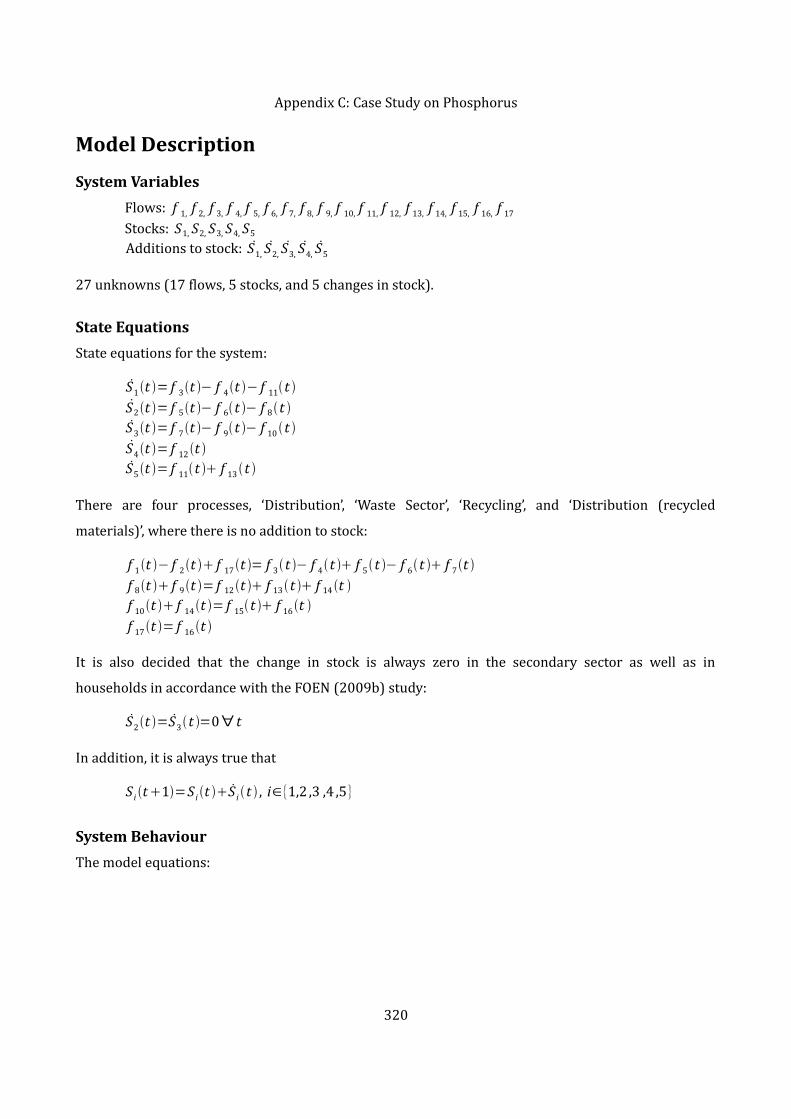
Appendix C: Case Study on PhosphorusModel DescriptionSystem VariablesFlows: f 1, f 2, f 3, f 4, f 5, f 6, f 7, f 8, f 9, f 10, f 11, f 12, f 13, f 14, f 15, f 16, f 17Stocks: S1, S2, S3, S4, S5Additions to stock: S1, S2, S3, S4, S527 unknowns (17 flows, 5 stocks, and 5 changes in stock). State EquationsState equations for the system:

S1t = f 3t − f 4t − f 11t S2t = f 5t − f 6t − f 8t S3t = f 7t − f 9t − f 10 t S4t = f 12 t S5t = f 11t f 13 t There are four processes, ‘Distribution’, ‘Waste Sector’, ‘Recycling’, and ‘Distribution (recycled materials)’, where there is no addition to stock: f 1t − f 2t f 17t = f 3t − f 4t f 5t − f 6t f 7t f 8t f 9t = f 12t f 13t f 14 t f 10t f 14t = f 15t f 16t f 17t = f 16t It is also decided that the change in stock is always zero in the secondary sector as well as in households in accordance with the FOEN (2009b) study:S2t =S3t =0∀ tIn addition, it is always true thatS i t1=S i t S i t , i∈{1,2 ,3 ,4 ,5}

System BehaviourThe model equations:

320

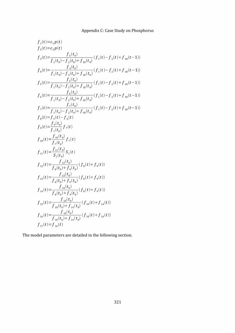
Appendix C: Case Study on Phosphorusf 1t =c1 pt f 2t =c2 pt

f 3t = f 3t0f 1t0− f 2t0 f 18 t 0 f 1t − f 2t f 18 t−1

f 4t = f 4t0f 1t 0− f 2t0 f 18 t0 f 1t − f 2t f 18 t−1

f 5t = f 5t0f 1t0− f 2t0 f 18 t 0 f 1t − f 2t f 18 t−1

f 6t = f 6t0f 1t 0− f 2t0 f 18 t 0 f 1t − f 2t f 18 t−1

f 7t = f 7t0f 1t0− f 2t0 f 18 t 0 f 1t − f 2t f 18 t−1

f 8t = f 5t − f 6t f 9t = f 9t0

f 7t0 f 7t f 10t = f 10 t 0

f 7t0 f 7t

f 11t = f 11 t 0S1t 0 S1t

f 12t = f 12t0f 8t0 f 9t0 f 8t f 9t

f 13t = f 13t0f 8t0 f 9t0 f 8t f 9t

f 14t = f 14t0f 8t0 f 9t0 f 8t f 9t

f 15t = f 15t0f 10t0 f 14t0 f 10 t f 14 t

f 16t = f 16t0f 10t0 f 14t0 f 10 t f 14 t

f 17t = f 16t The model parameters are detailed in the following section.

321

Appendix C: Case Study on PhosphorusModel Parameters

Table C.7: Phosphorus model parameters

Model Parameter

Parameter Description Constant Value If Constant

c1 The relation between apparent consumption and the Geneva populationYes (f1(t0) – f2(t0) + f18(t0))/p(t0)

p(t) The size of the population. Source: OCSTAT Not0 The starting year of the simulation Yes 2006

Initial ValuesThe initial stock and flow values used in the dynamic MFA model (source: the normalized scenarios). ‘-’ denotes scenario-dependent values.Table C.8: Phosphorus model variables

Stock/Flow

Value [t] Comments

f1(t0) - Imports to all the different economic sectors, rainfall includedf2(t0) - Animal feed exportsf3(t0) - Imports to the primary sector & flows from other economic sectors (animal feed (imp.), animals (imp.), mineral fertilizers (imp.), fodder soup)f4(t0) - Exports from the primary sector & flows to other economic sectors (animals & milk & eggs, animal feed (exp.), garden mineral fertilizers, domestic food of plant origin, domestic wood products, domestic wood energy)f5(t0) - Imports to the secondary sector & flows from other economic sectors (wood products (imp.), wood energy (imp.), paper (imp.), domestic wood products, domestic wood energy, food of animal origin (imp.), animals & milk & eggs, food of plant origin (imp.), domestic food of plant origin, chemicals (imp.), products (imp.))f6(t0) - Flows to other economic sectors (wood products, wood energy, paper, food of animal origin, food of plant origin, fodder soup, cleaning products)

322

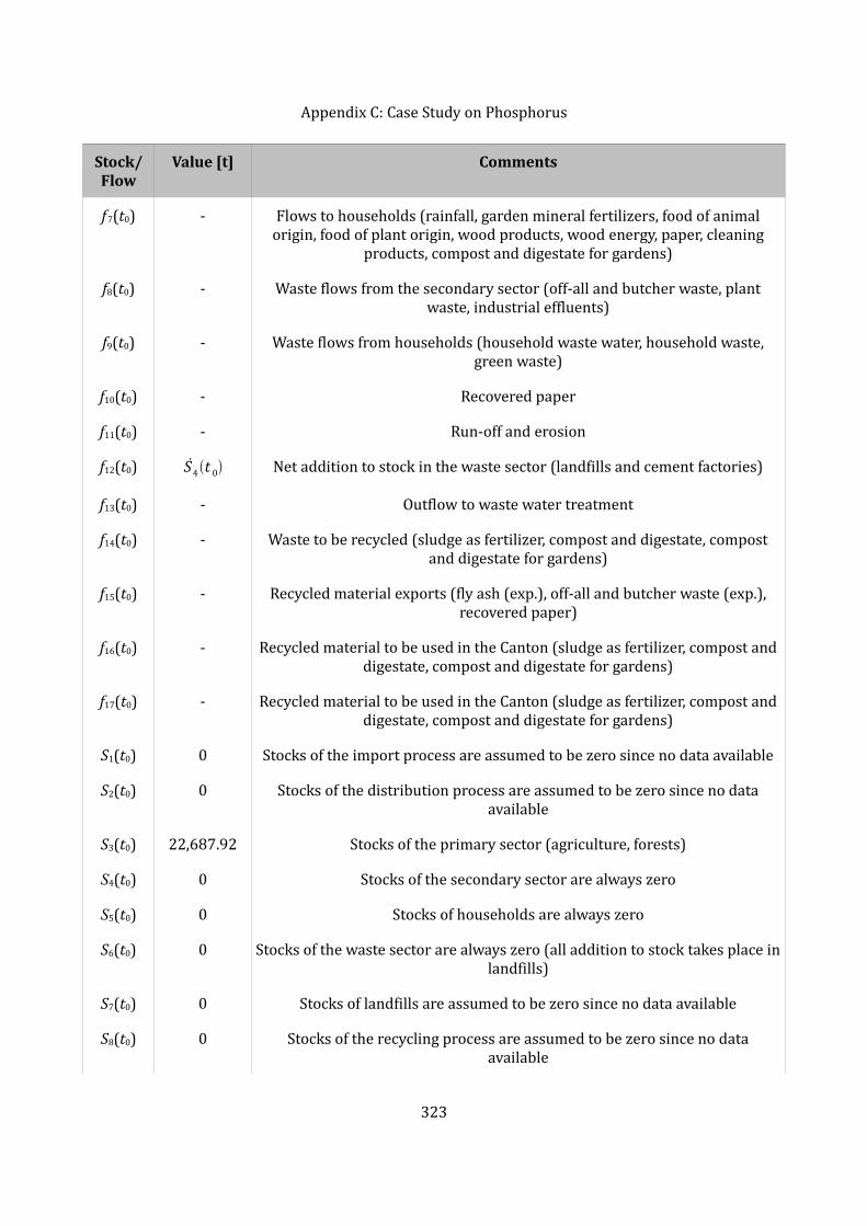
Appendix C: Case Study on PhosphorusStock/Flow

Value [t] Comments

f7(t0) - Flows to households (rainfall, garden mineral fertilizers, food of animal origin, food of plant origin, wood products, wood energy, paper, cleaning products, compost and digestate for gardens)f8(t0) - Waste flows from the secondary sector (off-all and butcher waste, plant waste, industrial effluents)f9(t0) - Waste flows from households (household waste water, household waste, green waste)f10(t0) - Recovered paperf11(t0) - Run-off and erosionf12(t0) S4t 0 Net addition to stock in the waste sector (landfills and cement factories)f13(t0) - Outflow to waste water treatmentf14(t0) - Waste to be recycled (sludge as fertilizer, compost and digestate, compost and digestate for gardens)f15(t0) - Recycled material exports (fly ash (exp.), off-all and butcher waste (exp.), recovered paper)f16(t0) - Recycled material to be used in the Canton (sludge as fertilizer, compost and digestate, compost and digestate for gardens)f17(t0) - Recycled material to be used in the Canton (sludge as fertilizer, compost and digestate, compost and digestate for gardens)S1(t0) 0 Stocks of the import process are assumed to be zero since no data availableS2(t0) 0 Stocks of the distribution process are assumed to be zero since no data availableS3(t0) 22,687.92 Stocks of the primary sector (agriculture, forests)S4(t0) 0 Stocks of the secondary sector are always zeroS5(t0) 0 Stocks of households are always zeroS6(t0) 0 Stocks of the waste sector are always zero (all addition to stock takes place in landfills)S7(t0) 0 Stocks of landfills are assumed to be zero since no data availableS8(t0) 0 Stocks of the recycling process are assumed to be zero since no data available

323

Appendix C: Case Study on PhosphorusStock/Flow

Value [t] Comments

S9(t0) 0 Stocks of ground and surface waters are always zero S10(t0) 0 Stocks of the distribution (recycled materials) process are assumed to be zero since no data availableS11(t0) 0 Stocks of the export (products)process are assumed to be zero since no data availableS12(t0) 0 Stocks of the export (recycled material) process are to be assumed zero since no data availableS3t0 - Change of stock in the primary sectorS4t 0 0 Change of stock in the secondary sector is always zeroS5t0 0 Change of stock in households is always zeroS7t0 - Change of stock in the waste sector

The used initial flow and change in stock values for the different scenarios are summarized in the following tables. The initial stock values correspond directly to the normalization results (see TableC.10). BaU = ‘Business as Usual’, MBF = ‘Meat and Bone Meal Fertilizer’, SSF = ‘Sewage Sludge Fertilizer’, RGW = ‘Recycling of Green Waste, URe = ‘Urine Recycling’, imp. = imports, exp. = exports.

324

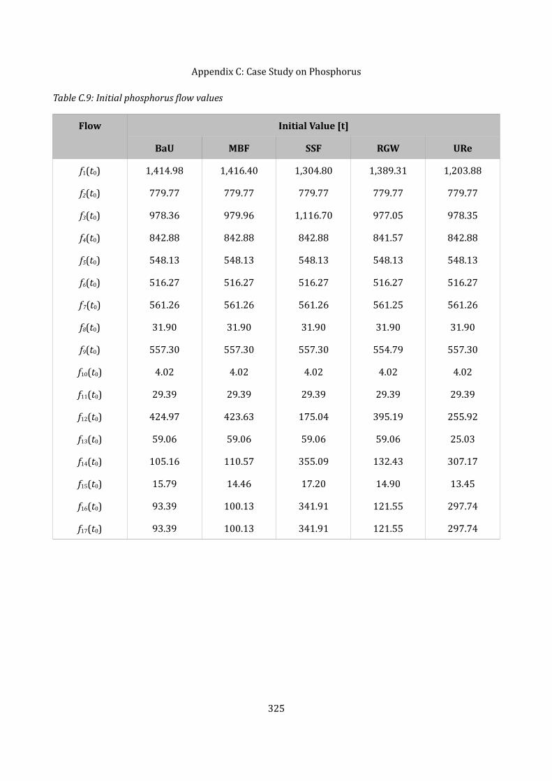
Appendix C: Case Study on PhosphorusTable C.9: Initial phosphorus flow values

Flow Initial Value [t]

BaU MBF SSF RGW URe

f1(t0) 1,414.98 1,416.40 1,304.80 1,389.31 1,203.88f2(t0) 779.77 779.77 779.77 779.77 779.77f3(t0) 978.36 979.96 1,116.70 977.05 978.35f4(t0) 842.88 842.88 842.88 841.57 842.88f5(t0) 548.13 548.13 548.13 548.13 548.13f6(t0) 516.27 516.27 516.27 516.27 516.27f7(t0) 561.26 561.26 561.26 561.25 561.26f8(t0) 31.90 31.90 31.90 31.90 31.90f9(t0) 557.30 557.30 557.30 554.79 557.30f10(t0) 4.02 4.02 4.02 4.02 4.02f11(t0) 29.39 29.39 29.39 29.39 29.39f12(t0) 424.97 423.63 175.04 395.19 255.92f13(t0) 59.06 59.06 59.06 59.06 25.03f14(t0) 105.16 110.57 355.09 132.43 307.17f15(t0) 15.79 14.46 17.20 14.90 13.45f16(t0) 93.39 100.13 341.91 121.55 297.74f17(t0) 93.39 100.13 341.91 121.55 297.74

325

Appendix C: Case Study on PhosphorusTable C.10: Initial phosphorus stock values

Change in Stock

Initial Value [t]

BaU MBF SSF RGW URe

S1t0 106.09 107.70 244.43 106.09 106.09S2t0 0.00 0.00 0.00 0.00 0.00S3t0 0.00 0.00 0.00 0.00 0.00S4t 0 424.97 423.63 175.04 554.79 255.92S5t0 88.45 88.45 88.45 88.45 88.45

Uncertainty AnalysisMinimal and Maximal ValuesThe maximal values correspond to the initial values of the ‘Business as Usual’ scenario multiplied by 2. The minimal values correspond to the initial values of the ‘Business as Usual’ scenario divided by 2. Uncertainty ScenariosThe uncertainty scenarios were defined by dividing the four categories:

– imports: flows f1, f3, f5, f 7– exports: flows f2, f4, f6– waste flows: flows f8, f9, f10, f12, f13, f14, f15, f16, f17 – water systems: flow f11There are in total 24 = 16 possible combinations of these groups of flows. All the scenarios were studied in the form of uncertainty scenarios listed below (‘*2’ denote maximal and ‘/2’ minimal values of the flows in question).In the implementation of the uncertainty analysis, it is also necessary to take into account the fact that in the system representation (Figure 5.12) the inflows to the economic sectors include not only imports but also goods from other economic sectors. For instance, the inflow to households includes imported food as well as food produced in the Canton’s secondary sector. The same is naturally true for the outflows to distribution; they include not only exports but also goods for consumption in the

326

Appendix C: Case Study on PhosphorusCanton. In addition, the economic sector inflows also include recycled materials (e.g. compost and digestate) used as fertilizer. All these flows need to be divided into components when necessary and each component should be treated in coherence with the uncertainty scenario in question.Table C.11: Uncertainty scenarios

Scenario Number Imports Exports Waste Flows

Water Systems

1 *2 *2 *2 *22 /2 *2 *2 *23 *2 /2 *2 *24 *2 *2 /2 *25 *2 *2 *2 /26 /2 /2 *2 *27 /2 *2 /2 *28 /2 *2 *2 /29 *2 /2 /2 *210 *2 /2 *2 /211 *2 *2 /2 /212 /2 /2 /2 *213 /2 /2 *2 /214 /2 *2 /2 /215 *2 /2 /2 /216 /2 /2 /2 /2

327

328

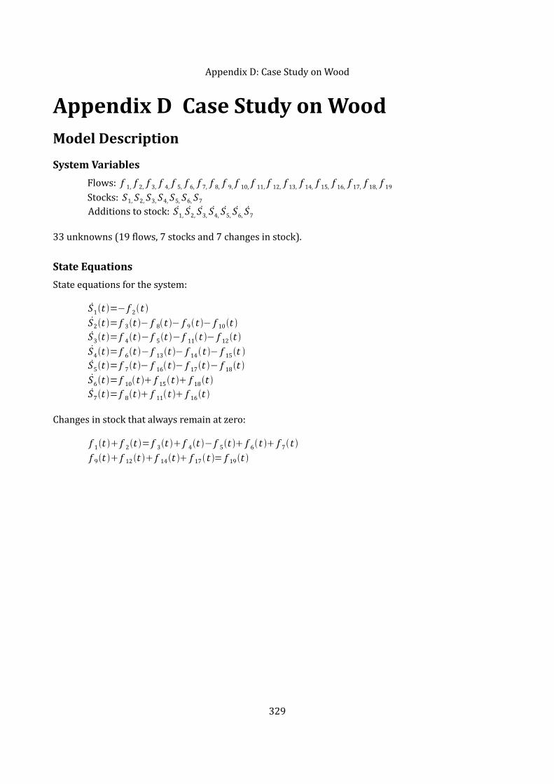
Appendix D: Case Study on WoodAppendix D Case Study on WoodModel DescriptionSystem VariablesFlows: f 1, f 2, f 3, f 4, f 5, f 6, f 7, f 8, f 9, f 10, f 11, f 12, f 13, f 14, f 15, f 16, f 17, f 18, f 19Stocks: S1, S2, S3, S4, S5, S6, S7Additions to stock: S1, S2, S3, S4, S5, S6, S733 unknowns (19 flows, 7 stocks and 7 changes in stock).State EquationsState equations for the system:

S1t =− f 2t S2t = f 3t − f 8t − f 9t − f 10t S3t = f 4t − f 5t − f 11t − f 12t S4t = f 6t − f 13t − f 14t − f 15t S5t = f 7t − f 16t − f 17t − f 18t S6t = f 10t f 15t f 18t S7t = f 8t f 11t f 16t Changes in stock that always remain at zero:f 1t f 2t = f 3t f 4t − f 5t f 6t f 7t f 9t f 12 t f 14t f 17t = f 19t

329

Appendix D: Case Study on WoodModel Equations

f 1t f 2t =c1 pt f 2t =c2f 3t = f 30

f 10 f 20 f 1t f 2t f 4t = f 40

f 10 f 20 f 1t f 2t f 5t = f 50

f 10 f 20 f 1t f 2t f 6t = f 60

f 10 f 20 f 1t f 2t f 7t = f 70

f 10 f 20 f 1t f 2t f 8t = f 80

f 80 f 90 f 30 f 10 f 20 G t

f 9t = f 90f 80 f 90 f 30

f 10 f 20 G t

f 10t =c3 f 10 f 20 f 10 f 20− f 40 f 50 f 30

f 10 f 20 f 1t f 2t f 11t = f 110

f 110 f 120 f 40− f 50 f 10 f 20G t

f 12t = f 120f 110 f 120 f 40− f 50

f 10 f 20G t

f 13t = f 130f 130 f 140 f 60

f 10 f 20G t

f 14t = f 140f 130 f 140 f 60

f 10 f 20G t

f 15t =c3 f 10 f 20 f 10 f 20− f 40 f 50 f 60

f 10 f 20 f 1t f 2t f 16t = f 160

f 160 f 170 f 70 f 10 f 20G t

f 17t = f 170f 160 f 170 f 70

f 10 f 20G t

f 18t =c3 f 10 f 20 f 10 f 20− f 40 f 50 f 70

f 10 f 20 f 1t f 2t f 19t = f 9t f 12t f 14t f 17t The model parameters are detailed in the following section.

330

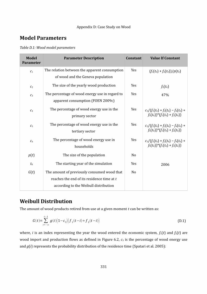
Appendix D: Case Study on WoodModel ParametersTable D.1: Wood model parameters

Model Parameter

Parameter Description Constant Value If Constant

c1 The relation between the apparent consumption of wood and the Geneva population Yes (f1(t0) + f2(t0))/p(t0)c2 The size of the yearly wood production Yes f2(t0)c3 The percentage of wood energy use in regard to apparent consumption (FOEN 2009c) Yes 47%c4 The percentage of wood energy use in the primary sector Yes c3/(f1(t0) + f2(t0) − f4(t0) +

f5(t0))*(f1(t0) + f2(t0)) c5 The percentage of wood energy use in the tertiary sector Yes c3/(f1(t0) + f2(t0) − f4(t0) +

f5(t0))*(f1(t0) + f2(t0)) c6 The percentage of wood energy use in households Yes c3/(f1(t0) + f2(t0) − f4(t0) +

f5(t0))*(f1(t0) + f2(t0)) p(t) The size of the population No

t0 The starting year of the simulation Yes 2006G(t) The amount of previously consumed wood that reaches the end of its residence time at t according to the Weibull distribution

No

Weibull DistributionThe amount of wood products retired from use at a given moment t can be written as:G t =∑

i=−∞

t−1gi 1−c3 f 1t−i f 2t−i (D.1)

where, i is an index representing the year the wood entered the economic system, f1(t) and f2(t) are wood import and production flows as defined in Figure 6.2, c3 is the percentage of wood energy use and g(i) represents the probability distribution of the residence time (Spatari et al. 2005): 331

Appendix D: Case Study on Woodg i=ai a−1

ba e− i

b

a (D.2)a is a shape parameter and b a scale parameter (for more information, see Spatari et al. 2005). g(i) gives the probability with which a product that entered use i years ago leaves the economic system. Initial Values ‘Business as Usual’The initial stock and flow values used in the dynamic MFA model are presented here. Table D.2: Initial wood stock and flow values, ‘Business as Usual’ scenario

Stock/Flow

Value [t] Comments

f1 216,700 Corresponds to 222,100 t of apparent consumption from normalized FOEN (2009b) study – f2 f2 5,400 Source: Faessler et al. (2010)f3 12,399 Calculated based on the total wood inputs f1 + f2 and the relative size of the sectorial flow (Faist Emmenegger & Frischknecht 2003)f4 44,204 Idem.f5 14,555 Idem.f6 83,557 Idem.f 7 96,495 Idem.f8 2,537 Calculated based on the total amount of incinerated waste f8 + f11 + f13 + f16 (29,600

t (Faessler et al. 2010)) and the relative size of the sectorial flow (Faist Emmenegger & Frischknecht 2003)

f9 333 Calculated based on the total recycled waste f19 and the relative size of the sectorial flow (Faist Emmenegger & Frischknecht 2003)f11 2,537 Calculated based on the total amount of incinerated waste f8 + f11 + f13 + f16 29,600 t (Faessler et al. 2010) and the relative size of the sectorial flow (Faist Emmenegger & Frischknecht 2003)f12 1,480 Calculated based on the total recycled waste f19 and the relative size of the sectorial flow (Faist Emmenegger & Frischknecht 2003)f13 10,149 Calculated based on the total amount of incinerated waste f8 + f11 + f13 + f16 29,600 t (Faessler et al. 2010) and the relative size of the sectorial flow (Faist Emmenegger & Frischknecht 2003)

332

Appendix D: Case Study on WoodStock/Flow

Value [t] Comments

f14 2,664 Calculated based on the total recycled waste f19 and the relative size of the sectorial flow (Faist Emmenegger & Frischknecht 2003)f16 14,377 Calculated based on the total amount of incinerated waste f8 + f11 + f13 + f16 29,600 t (Faessler et al. 2010) and the relative size of the sectorial flow (Faist Emmenegger & Frischknecht 2003)f17 1,924 Calculated based on the total recycled waste f19 and the relative size of the sectorial flow (Faist Emmenegger & Frischknecht 2003)f19 64,000 Source: Faessler et al. (2010)S1 413,000 Source: Faessler et al. (2010)S2 66,000 Source: Faist Emmenegger & Frischknecht (2003)S3 122,000 Source: Faist Emmenegger & Frischknecht (2003)S4 332,000 Source: Faist Emmenegger & Frischknecht (2003)S5 820,000 Source: Faist Emmenegger & Frischknecht (2003)S6 0 Assumed at zero since no data availableS7 0 Source: Faist Emmenegger & Frischknecht (2003)

Adjusted Values ‘Business as Usual’The adjusted flow values used in the dynamic MFA model are presented here. The stock values as well as the waste and wood energy flow values are identical to those initially used.

333

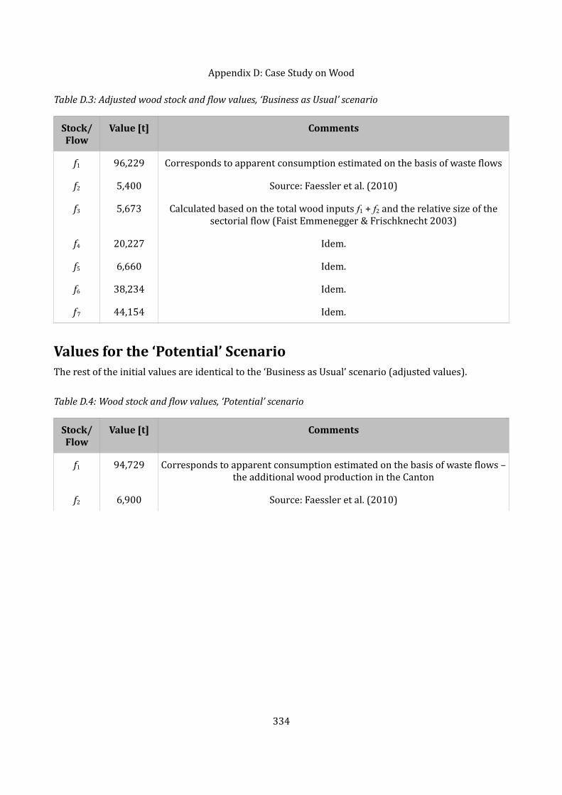
Appendix D: Case Study on WoodTable D.3: Adjusted wood stock and flow values, ‘Business as Usual’ scenario

Stock/Flow

Value [t] Comments

f1 96,229 Corresponds to apparent consumption estimated on the basis of waste flowsf2 5,400 Source: Faessler et al. (2010)f3 5,673 Calculated based on the total wood inputs f1 + f2 and the relative size of the sectorial flow (Faist Emmenegger & Frischknecht 2003)f4 20,227 Idem.f5 6,660 Idem.f6 38,234 Idem.f7 44,154 Idem.

Values for the ‘Potential’ Scenario The rest of the initial values are identical to the ‘Business as Usual’ scenario (adjusted values).Table D.4: Wood stock and flow values, ‘Potential’ scenario

Stock/Flow

Value [t] Comments

f1 94,729 Corresponds to apparent consumption estimated on the basis of waste flows – the additional wood production in the Cantonf2 6,900 Source: Faessler et al. (2010)

334

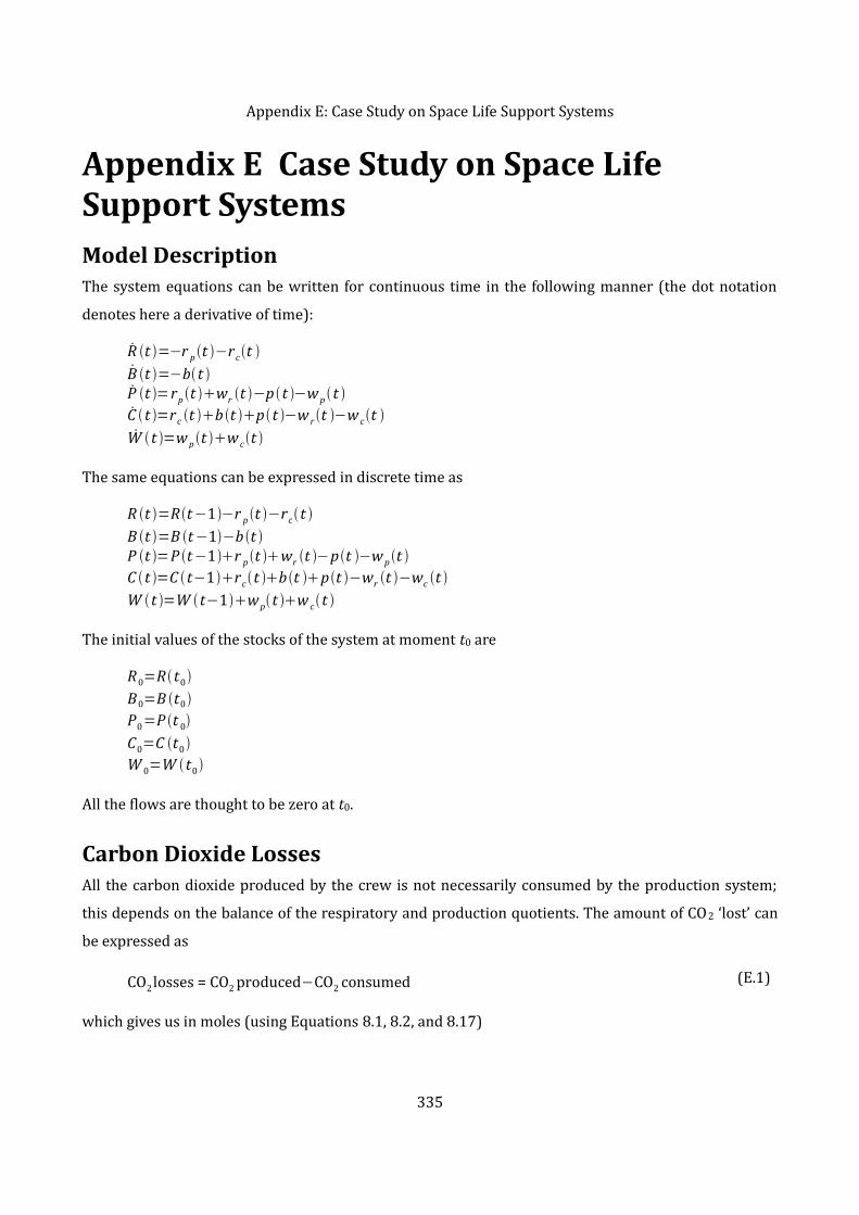
Appendix E: Case Study on Space Life Support SystemsAppendix E Case Study on Space Life Support SystemsModel DescriptionThe system equations can be written for continuous time in the following manner (the dot notation denotes here a derivative of time):

R t =−r p t −rct B t =−bt P t =rp t wr t −pt −w p t C t =rc t b t pt −w rt −w ct W t =w p t w ct The same equations can be expressed in discrete time asR t =Rt−1−r pt −rct B t =B t−1−b t P t =P t−1r pt wr t −pt −w pt C t =C t−1rct bt pt −wr t −wc t W t =W t−1wpt w ct The initial values of the stocks of the system at moment t0 areR 0=Rt0B0=B t0P0=P t 0C0=C t0W 0=W t0All the flows are thought to be zero at t0.

Carbon Dioxide LossesAll the carbon dioxide produced by the crew is not necessarily consumed by the production system; this depends on the balance of the respiratory and production quotients. The amount of CO2 ‘lost’ can be expressed asCO2losses = CO2 produced−CO2 consumed (E.1)which gives us in moles (using Equations 8.1, 8.2, and 8.17)335

Appendix E: Case Study on Space Life Support SystemsCO2losses [mol]= QR

NC− 1

QP pt

M 1 (E.2)and again in grams

CO2losses [g]= QR

NC− 1

QPM 2

M 1 pt (E.3)M1 and M2 are the molar masses of oxygen and carbon dioxide. The amount of carbon dioxide [g] transformed by the air regeneration system can be written as

w trsf=1QP

M2M1 pt (E.4)

Solved Systemr pt =NC⋅RI P⋅nt rc t =RIC⋅nt bt =1−NC⋅nt pt =NC⋅nt w r t =1−WICRI C⋅nt w p t =NC⋅RI P−11−WICRIC ⋅nt w ct =WIC⋅nt With these flow values, the stocks can now be determined iteratively with the knowledge of initial stock values.

Simulation ResultsThe simulation results are shown here in the form of screen shots from the MS Excel simulation model.ARES Simulation with Original Reference MissionThere are some rounding errors in the ARES model; these errors result from inaccuracies in the original material flow analysis.

336

Appendix E: Case Study on Space Life Support Systems

337

Figure E.1: Common input parameters, ARES

Appendix E: Case Study on Space Life Support Systems

Figure E.2: Oxygen simulation, ARES

338

Appendix E: Case Study on Space Life Support Systems

Figure E.3: Total mass simulation, ARES

339

Appendix E: Case Study on Space Life Support SystemsBIORAT Simulation with Original Reference Mission

340

Figure E.4: Common input parameters, BIORAT

Appendix E: Case Study on Space Life Support Systems

Figure E.5: Oxygen simulation, BIORAT

341

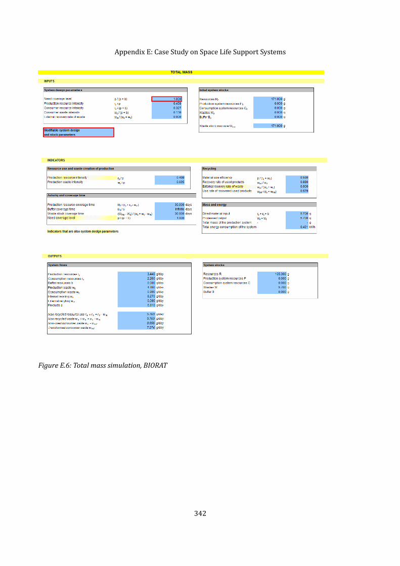
Appendix E: Case Study on Space Life Support Systems

Figure E.6: Total mass simulation, BIORAT

342

Appendix E: Case Study on Space Life Support SystemsBIORAT Simulation with ARES Reference Mission

343

Figure E.7: Common input parameters, redimensioned BIORAT

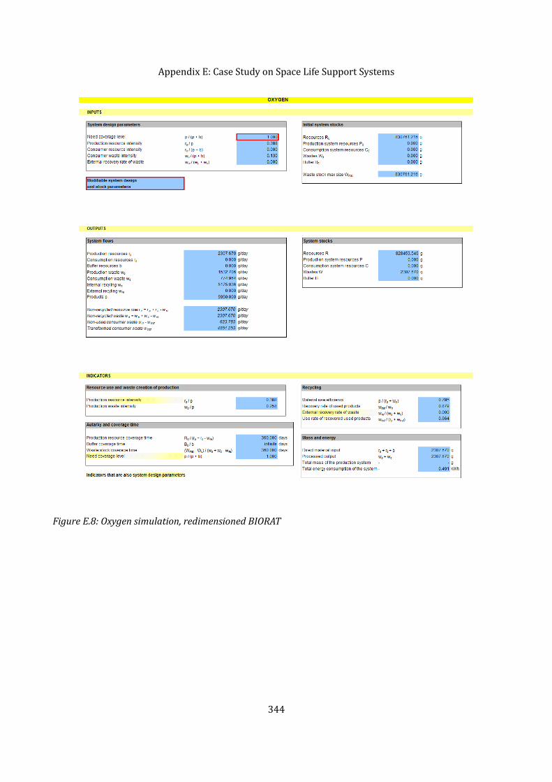
Appendix E: Case Study on Space Life Support Systems

Figure E.8: Oxygen simulation, redimensioned BIORAT

344

Appendix E: Case Study on Space Life Support Systems

Figure E.9: Total mass simulation, redimensioned BIORAT

345

346

Appendix F: RecommendationsAppendix F RecommendationsPolicy recommendations marked with a question mark (‘?’) denote that the option can neither be proved nor disproved based on our analysis. Potential means to accomplish the recommended evolutions are listed as well as unresolved issues that need to be closely examined before making the final decision. The list of policy instruments is by no means intended to be exhaustive. For more information on policy instruments and their functioning, see, for example, Sterner (2003).

347

Appendix F: RecommendationsTable F.1: Policy recommendations for copper

Policy Question Recommended Action Policy Instruments

Consequences for Resource Use Issues to be Elucidated/Other RemarksWhich of the scenarios ‘90% Recycling of Building Waste’ and ‘Substitution in Roofing and Guttering’ has greater effect?

Substitution in roofing and guttering Subsidies, regulations Decrease in copper imports (-43% vs. -16% in cumulated imports); increase in the imports of substituting substancesEnvironmental impacts of substituting substances

Should the transition to e-mobility be encouraged? Yes Subsidies, regulations Slightly increased copper use (+5% consumption per capita) Environmental impacts of e-mobility; scarcity of other e-mobility substances (e.g. lithium)Is the ‘No Primary Copper’ scenario feasible? ? Subsidies, regulations, taxation Decrease in copper imports and in copper consumption (consumption per capita -63% in 2080)Should copper recycling be encouraged? Yes Subsidies, regulations, taxation Decrease in copper imports Environmental impacts of recyclingShould copper substitution with other substances be encouraged? ? (Substitution with renewable resources might be recommended) Subsidies, regulations, taxation Decrease in copper imports; Increase in the imports of other substances Environmental impacts of substituting substances; scarcity of substituting substancesShould the exploitation of anthropogenic mines be encouraged? ? Subsidies, regulations, taxation Decrease in copper imports Replacement of in-use copper with other substances

348

Appendix F: RecommendationsTable F.2: Policy recommendations for phosphorus

Policy Question Recommended Action Policy Instruments Consequences for Resource Use

Issues to be Elucidated/Other RemarksWhich one of the FOEN scenarios (‘Sewage Sludge’, ‘Meat and Bone Meal’, or ‘Green Waste’) should be favoured on the Geneva level?

In terms of minimizing copper imports, the scenario ‘Sewage Sludge as Fertilizer’ should be favouredSubsidies, regulations Decrease in phosphorus imports (-15% in cumulated imports) Environmental and health impacts of the scenario

Should human urine recycling as fertilizer be encouraged? Yes Subsidies Decrease in phosphorus imports (-34% in cumulated imports) Environmental and health impacts of urine recyclingHow to prevent phosphorus accumulation in ground and surface waters? Reduce inflow from waste sector (e.g. by human urine recycling) or reduce run-off from agriculture (avoid over-fertilization)

Regulations Decrease in phosphorus in ground and surface waters (urine recycling: phosphorus addition to water systems -43%)Environmental and health impacts

Should phosphorus recycling be encouraged? Yes Subsidies, regulations, taxation Decrease in phosphorus imports Environmental impacts of recyclingShould investments in phosphorus capture technology (from waste water) be encouraged?? Subsidies Decrease in phosphorus in ground and surface waters; decrease in phosphorus imports

Development costs and feasibility of the technology

349

Appendix F: RecommendationsTable F.3: Policy recommendations for wood

Policy Question Recommended Action

Policy Instruments Consequences for Resource Use Issues to be Elucidated/Other RemarksShould the Canton’s forest exploitation be encouraged? Yes Subsidies Decrease in wood imports (‘potential’ scenario: -2% in cumulated imports) Less transport

Should the use of local wood (from the greater Geneva agglomeration) be encouraged? Yes Subsidies, taxation, regulations, labels Decrease in long-distance wood imports Geneva represents 52% of the population but only 3% of exploitable resources (Faessler et al. 2010); less transportShould a transition from wood energy to wood products for Geneva wood be encouraged? ? Subsidies Decrease in wood product imports; increase in energy imports Is wood energy of Genevan origin replaced by wood energy imports or by other energy sources; potential for higher value-added productsShould wood heating be encouraged? ? Subsidies Increase in wood imports; decrease in other energy imports Wood fuel preferable compared to fossil fuelsShould the recycling of wood waste (as opposed to incineration) be encouraged? ? Subsidies, regulations Decrease in wood product imports; potential increase in energy imports Environmental impacts of recycling; potential for higher value-added productsShould the local exploitation of recycled wood (as opposed to exporting it) be encouraged? ? Subsidies, taxation, regulations Decrease in wood imports Feasibility of local exploitation; less transportShould the use of wood as opposed to non-renewable materials be encouraged? Yes Subsidies, regulations Increase in wood imports; decrease in imports of non-renewable materials Environmental impacts of wood use

350

Appendix F: RecommendationsTable F.4: Policy recommendations for lithium

Policy Question Recommended Action

Policy Instruments Consequences for Resource Use Issues to be Elucidated/Other RemarksShould recycling of lithium batteries be encouraged? Yes Subsidies, regulations, national & international policies Decrease in primary lithium consumption Environmental impacts of recycling; appropriate scale for recycling (regional/national/supranational)Should the transition to e-mobility be encouraged? ? Subsidies, taxation, regulations Increase in lithium consumption (in order to replace ICE vehicles with EVs in Geneva, 21 kt of lithium are needed)

Environmental impacts of e-mobility (lithium extraction); decrease in fossil fuel consumptionShould the development of alternative (non-lithium) battery technologies be encouraged?

? Subsidies Decrease in lithium consumption; Increase in the consumption of substituting substances Environmental impacts of non-lithium batteries; costs and performance of the technology; scarcity of the substituting substancesShould green mobility (walking, cycling, car-sharing) be encouraged? Yes Subsidies, taxation, tolls Decrease in lithium consumption Overall development plan for ‘soft’ mobility is being prepared (Canton of Geneva 2011f)Should a less mobile lifestyle (living closer to one’s workplace etc.) be encouraged?? Subsidies, taxation, tolls Decrease in transportation needs Feasibility and acceptability of lesser mobility; potential for mobility reduction in densely populated Geneva

351