THE ASTROPHYSICAL JOURNAL, 474 :223È255, 1997 January 11997. The American Astronomical Society. All rights reserved. Printed in U.S.A.(

DESTRUCTION OF THE GALACTIC GLOBULAR CLUSTER SYSTEM

OLEG Y. AND JEREMIAH P.GNEDIN OSTRIKER

Princeton University Observatory, Peyton Hall, Princeton, NJ 08544 ; ognedin=astro.princeton.edu, jpo=astro.princeton.eduReceived 1996 February 15 ; accepted 1996 July 24

ABSTRACTWe investigate the dynamical evolution of the Galactic globular cluster system in considerably greater

detail than has been done hitherto, Ðnding that destruction rates are signiÐcantly larger than given byprevious estimates. The general scheme (but not the detailed implementation) follows Aguilar, Hut, &Ostriker.

For the evolution of individual clusters, we use a Fokker-Planck code including the most importantphysical processes governing the evolution : two-body relaxation, tidal truncation of clusters, compressivegravitational shocks while clusters pass through the Galactic disk, and tidal shocks due to passage closeto the bulge. Gravitational shocks are treated comprehensively, using a recent result by Kundic� &Ostriker that the S*E2T shock-induced relaxation term, driving an additional dispersion of energies, isgenerally more important than the usual energy shift term S*ET. Various functional forms of the correc-tion factor are adopted to allow for the adiabatic conservation of stellar actions in a presence of tran-sient gravitational perturbation.

We use a recent compilation of the globular cluster positional and structural parameters, and a collec-tion of radial velocity measurements. Two transverse to the line-of-sight velocity components wereassigned randomly according to the two kinematic models for the cluster system (following the methodof Aguilar, Hut, & Ostriker) : one with an isotropic peculiar velocity distribution, corresponding to thepresent-day cluster population, and the other with the radially preferred peculiar velocities, similar tothose of the stellar halo. We use the Ostriker & Caldwell and the Bahcall, Schmidt, & Soneira modelsfor our Galaxy.

For each cluster in our sample, we calculated its orbits over a Hubble time, starting from the presentobserved positions and assumed velocities. Medians of the resulting set of peri- and apogalactic distancesand velocities are used then as an input for the Fokker-Planck code. Evolution of the cluster is followedup to its total dissolution due to a coherent action of all of the destruction mechanisms. The rate ofdestruction is then obtained as a median over all the cluster sample, in accord with Aguilar, Hut, &Ostriker.

We Ðnd that the total destruction rate is much larger than that given by Aguilar, Hut, & Ostrikerwith more than half of the present clusters (52%È58% for the Ostriker & Caldwell model, and 75%È86%for the Bahcall, Schmidt, & Soneira model) destroyed in the next Hubble time. Alternatively put, thetypical time to destruction is comparable to the typical age, a result that would follow from (but is notrequired by) an initially power law distribution of destruction times. We discuss some implications for apast history of the globular cluster system and the initial distribution of the destruction times, raising thepossibility that the current population is but a very small fraction of the initial population with theremnants of the destroyed clusters constituting presently a large fraction of the spheroid (bulge ] halo)stellar population.Subject headings : celestial mechanics, stellar dynamics È Galaxy : kinematics and dynamics È

globular clusters : general

1. INTRODUCTION

Globular clusters are thought to be the oldest stellarsystems in our Galaxy, and a history of attempts by theo-reticians and observers to understand the keys of their evo-lution is as old as the discipline of stellar dynamics, with acomprehensive review provided by Yet, theseSpitzer (1987).relatively simple stellar systems are not understood wellenough to predict their future with desirable accuracy, inpart due to lack of accurate observational values for thecurrent dynamical state and in part due to a residual uncer-tainty concerning the complete catalog of relevant physicalprocesses operating on these systems. More than that, wehave almost no clues about their past, and in particular,whether what we see now is representative of the initialglobular cluster system, or just a small leftover after a greatdestruction battle that occurred earlier in the history of theGalaxy. In this paper we consider the evolution of the

globular clusters and their ultimate disappearance andpropose a simple model for their initial distribution.

PreÈ and postÈcore collapse evolution of an isolatedcluster is relatively well understood (Spitzer 1987 ;

SigniÐcant progress in understanding ofGoodman 1993).the evolution was achieved using Monte Carlo and Fokker-Planck calculations. But the galactic environment makesthe clusters subject to external perturbationsÈtidal trunca-tion and the gravitational shocks due to passages close tothe bulge and through the disk. The shock processes,although known to be important, have never been carefullyincluded in the evolution of the system. We investigate theFokker-Planck models including the shocks elsewhere

Lee, & Ostriker hereafter and show(Gnedin, 1997a, GLO)that the dispersion of energy of the stars, induced by theshocks & 1995, hereafter is generally(Kundic� Ostriker KO),even more important for the evolution than the Ðrst-order

223

224 GNEDIN & OSTRIKER Vol. 474

energy shift. Another very important aspect of modelingglobular clusters is the initial mass spectrum. Multimassclusters undergo core collapse much faster than in thesingle-mass case, and their destruction is much more effi-cient (see & Goodman and the references inLee 1995,

We restrict ourselves, however, to the single-massGLO).models in order to maintain clear physical understanding,but owing to omission of this aspect of the problem, ourresults provide a lower bound to the rate of destruction ofthe globular clusters.

As long as we have (at least, an approximate) understand-ing of the evolution of a single cluster, we can turn to thestudy of the system of globular clusters in our Galaxy andin external galaxies. Kochanek, & ShapiroCherno†, (1986)used a semianalytical Monte Carlo technique to estimatethe importance of the di†erent mechanisms acting upon thecluster. They considered two-body relaxation, tidal strip-ping of stars, and the Ðrst-order tidal shocking e†ectÈdueto the disk crossing and interactions with giant molecularclouds (GMCs). For each of those processes, they calculatedthe cluster mass and energy changes associated with themto predict the evolution. They followed the cluster evolutiononly up to core collapse and assumed a single-mass Kingmodel for the internal structure of the cluster.(King 1966)Tidal heating due to the GMCs was found to be negligiblecompared to the disk shocks. Note, however, that theGalactic model assumed in that work Schmidt, &(Bahcall,Soneira hereafter is strongly favorable to the1983, BSS)disk shock for the clusters with small galactocentric radiussince the surface density of the disk increases exponentiallyas the radius decreases (see Cherno† et al. (1986)° 2.2).concluded that many of the clusters located within inner 3kpc from the Galactic center have undergone core collapseand that many of them may already have been destroyed. Anumber of authors have pointed out that the bulge andstellar spheroid themselves could be composed of remnantsof the destroyed globular clusters, if prior destruction ofglobular clusters occurred at high enough rate.

Another mechanism for the mass loss is stellar evolution.& Shapiro used a method similar to that ofCherno† (1987)

Cherno† et al. (1986) and included a power-law initial massfunction for the cluster stars. Mass loss due to stellar evolu-tion is important for the early evolution of the cluster butthen fades away because the mass loss is large only formassive stars whose lifetime is short. Comprehensive studyincluding the e†ects of stellar evolution has been done by

& Weinberg They used a Fokker-PlanckCherno† (1990).code with an extensive spectrum of stellar masses (20species), which includes stellar evolution and relaxationprocesses. Multimass models evolve much faster, and theevaporation rate is larger. Also, mass segregation (Spitzer

speeds up core collapse. Mass loss during Ðrst 5 ] 1091987)yr is sufficiently strong to disrupt weakly concentrated clus-ters (c\ 0.6). Combined with the relaxation, it destroysmany low-mass and low-concentration clusters within aHubble time.

The present characteristics and the evolutionary state ofthe observed Galactic globular clusters were also investi-gated by Hut, & Ostriker hereafterAguilar, (1988, AHO).We will draw heavily on that paper and compare our resultswith used a sample of the 83 Galactic globularAHO. AHOclusters with known structural parameters and line-of-sightvelocities. They considered virtually all the importantphysical mechanisms (except the mass spectrum and mass

loss due to stellar evolution) to calculate the present-daydestruction rates for the clusters in the sample. The rateswere deÐned as the inverse time it takes for a given mecha-nism to dissolve a cluster, in units of a Hubble time, which isnominally deÐned as 1010 yr. They estimated the rates forevaporation through the tidal boundary, disk and bulgetidal shocks, and dynamical friction. The last process hasnot been widely investigated in its application for the clusterevolution. Its e†ect reduces to gradual spiraling of thecluster toward the Galactic center, as the cluster losesorbital energy owing to continuous interactions with Ðeldstars and dark halo. found that this mechanism is aAHOrelatively unimportant one, except for unusually massiveclusters. They calculated a number of orbits associated witheach cluster in the sample and took a median over thewhole resulting distribution for a corresponding destructionrate. They investigated two galactic models &(OstrikerCaldwell hereafter and and two kine-1983, OC BSS; ° 2.2)matic models for the globular cluster system: isotropic,which corresponds to the current distribution, and pre-dominantly radial, which resembles that of the halo starsand which might be closer to an initial cluster distribution.The assumption concerning the velocity distribution isnecessary as only one velocity component is observed.(Note that the program to obtain true space velocities ofglobular clusters is underway ; & 1993).Cudworth HansonWe discuss the kinematic models in ° 2.3.

The central bulge was found to be very efficient indestroying clusters on highly elongated orbits. This leads toan isotropization of the orbits and even preferential survivalof tangentially biased orbits in the Hubble time. Thus, aninitially radial distribution better Ðts the present populationthan the initially isotropic one. At the current time, evapo-ration is the most important destruction process. The di†er-ence between the two galactic models was found to berelatively small, except for the disk shocking that obviouslydepends on the body of the surface mass proÐle. AHOintroduced a weighting factor that accounts for the fact thatsome orbits are less probable because of the variousdestruction mechanisms acting upon the cluster. Such aweighting reduces the computed rates but converges to asimilar value of 0.05 for all galactic models and kinematicproÐles considered. This implies that only four or Ðve clus-ters are destroyed over a Hubble time for the present condi-tions. But treated clusters in a simpliÐed fashion asAHOKing models, and they (like other investigators) did notallow for the tidal shock relaxation phenomena. It is thesedefects that we remedy in the present paper.

Ostriker, & Aguilar investigated the e†ect ofLong, (1992)the bar in our Galaxy on the destruction of the globularclusters. Barred orbits can bring the clusters close to theGalactic center where they are efficiently destroyed.However, only a small increase in the destruction rate wasdetected. Therefore, we did not consider the bar in thiswork.

Finally, a recent paper by & Djorgovski usedHut (1992)a statistical approach and approximate analytical estimatesfor the relaxation times for a sample of 140 clusters. Theyconcluded that the current evaporation rate is 5 ^ 3 Gyr~1(about 10 times the rate found by which means thatAHO),a signiÐcant fraction of the present-day clusters would bedestroyed in the next Hubble time.

In this paper we make a signiÐcant improvement overby applying detailed Fokker-Planck calculations toAHO

No. 1, 1997 GALACTIC GLOBULAR CLUSTER SYSTEM 225

the globular cluster sample. We describe the sample in ° 2.1and the galactic models in Then we discuss the two° 2.2.kinematic models and compare the resulting properties ofthe orbits for our sample. In we describe the destruc-° 2.5,tion mechanisms involved in the globular cluster evolution.We conclude with the history of our code and the formu-° 2lation of the numerical strategy. presents ourSection 3results for all runs. Finally, we speculate on the possiblepast history and future fate of the Galactic globular clustersin sums up our conclusions.° 4. Section 5

2. METHOD

2.1. Observational DataWe have used a recent compilation of globular cluster

coordinates by & Meylan and distancesDjorgovski (1993)and absolute magnitudes from (1993). ClusterDjorgovskiconcentrations, core radii, and half-mass radii were takenfrom Djorgovski, & King The core-collapsedTrager, (1993).clusters were assigned a limiting concentration of c\ 2.5.We used a constant mass-to-light ratio to obtain the clustermasses, in solar units 1993).(M/L )

V\ 3 (Djorgovski

We selected 119 clusters of 143 with available photo-metric data. All clusters in our sample have measured radialvelocities, which we collected from several sources.

& (1993) have derived actual spaceCudworth Hansonvelocities for 14 clusters, but we chose not to use those datato maintain homogeneity of the sample. We assign twounknown velocity components to each cluster using ourstatistical method in ° 2.3.

The observed parameters of our sample are given inThe Ðrst two columns are the sequential numberTable 1.

and clusterÏs name. The next two columns are the Galacticcoordinates. D is the distance of the cluster from the Sun inkiloparsecs, and R is the galactocentric radius. The seventhcolumn is concentration followed by corec\ log (R

t/R

c),

radius in parsecs. Tidal radius was calculated from theRc

Rtprevious two quantities. The next column is the cluster mass

converted from its luminosity. The last two columns are theline-of-sight velocities and the reference numbers to varioussources. The references are listed in at the end of Table 1.

2.2. Galactic ModelTo evaluate the gravitational shocks on the clusters we

have used two models for our Galaxy : the modelOCD-150, and the model. present a detailed com-BSS AHOparison between the two models. In the model, the diskOCis represented as the di†erence of two exponentials thatvanishes at the center, whereas disk density risesBSSÏsmonotonically as R decreases. The model has also aBSScompact nuclear component within 1 central kpc. Thus,both disk and bulge shocks are expected to be more(° 2.5)prominent for the model. As suggested by weBSS AHO,consider the di†erence of the results for the two models as ameasure of uncertainty associated with the distribution ofmass within the Galaxy.

We use the same routine to compute the Galactic modelas was done by The routine was kindly provided toAHO.us by L. Aguilar.

2.3. V elocity Distribution for the Globular Cluster SystemKinematic models for the Galactic globular cluster

system (GCS) have been sought widely in the past (see, e.g.,

& White & WhiteFrenk 1980 ; Thomas 1989). Frenk (1980)studied a sample of 66 clusters and found no evidence forthe radial expansion of the GCS as a whole. Their best Ðt toobserved kinematic distribution is that with the isotropicvelocity dispersion rising with the galactocentric distance asR0.2. An isotropic and isothermal (with constant velocitydispersion) model is still consistent with their data at the90% conÐdence level. Later work by Thomas (1989)included 115 clusters and conÐrmed the absence of theexpansion. He found that within the inner 7 kpc to theGalactic center, the velocity distribution is isotropic, but forthe outer radii, the velocity ellipsoid with slightly increasingline-of-sight dispersion may be preferred. Rotation velocityestimates and line-of-sight velocity dispersions as well astheir errors for both sources are given in Table 2.

We repeated the analysis of the velocity distributionusing our sample. We adopted the solar motion relative tothe LSR of ([9, 12, 7) km s~1 & Binney 1981, p.(Mihalas

and the circular velocity of the LSR of 220 km s~1.400)Line-of-sight projections of the two velocities were sub-tracted from the observed radial velocities to obtain rela-v

rtive to an inertial frame. Then the rotation velocity and itsuncertainty were estimated using equations (15) and (16) of

After subtraction of the rotation velocityThomas (1989).along the line of sight, we end up with the peculiar velocitieswith (presumably) zero mean. Both our and are invrot plosagreement with the above results within errors. Ouradopted values are also summarized in Table 2.

Following we investigate two initial kinematicAHOmodels for the globular cluster system. The Ðrst has anisotropic peculiar velocity distribution with constant veloc-ity dispersion. This is the simplest model still consistentwith the observations. We used the one-dimensional disper-sion of 118 km s~1, resulting from our sample.

The second model is anisotropic with velocity ellipsoidaxis ratio at solar position kpc similar to ther

_\ 8.5

spheroid stellar Population II :

pr2

pt2 \ 1 ] r2

ra2 , (1)

where and are the one-dimensional dispersions radialpr

ptand transverse to the Galactic center, respectively. We have

adopted the value of the anisotropy radiusAHO ra\

(0.8)1@2 kpc. Cluster orbits for this distribution arer_

B 7.6nearly isotropic within and become more and more radialr

awith increasing distance from the center.The amplitude of the radial velocity dispersion can be

obtained from the Jeans equation for the constant circularvelocity potential. Integration of the Jeans equation inspherical coordinates gives (see, e.g., Ogorodnikov 1965)

dopr2

dr] o

r(2p

r2[ 2p

t2[ vrot2 ) \ [o

vcirc2r

. (2)

For the velocity ellipsoid given by and theequation (1)power-law density proÐle o P r~a, we obtain

pr2\ (vcirc2 [ vrot2 )

[r2/(a [ 2)]] (ra2/a)

r2 ] ra2 . (3)

We accept km s~1 as the standard value for thevcirc \ 220circular velocity. found a \ 3.5 for hisThomas (1989)

TABLE 1

GLOBULAR CLUSTER PARAMETERS

l b D R Rc

Rt

M VrID Name (deg) (deg) (kpc) (kpc) c (pc) (pc) (M

_) (km s~1) References

1 . . . . . . . NGC 0104 305.90 [44.89 4.6 7.8 2.04 0.50 54.8 1.45e]06 [19.0 12 . . . . . . . NGC 0288 152.28 [89.38 8.3 11.9 0.96 3.47 31.6 1.11e]05 [46.0 13 . . . . . . . NGC 0362 301.53 [46.25 8.5 9.6 1.94 0.43 37.5 3.78e]05 223.2 14 . . . . . . . NGC 1261 270.54 [52.13 15.9 18.0 1.27 1.82 33.9 3.26e]05 51.0 25 . . . . . . . Pal 1 130.07 19.03 13.7 20.1 1.50 0.60 19.0 2.54e]03 3.0 26 . . . . . . . AM 1 258.36 [48.47 124.7 126.1 1.23 4.57 77.6 1.81e]04 116.0 37 . . . . . . . Eridanus 218.11 [41.33 79.5 84.8 1.10 5.89 74.2 2.30e]04 [21.0 38 . . . . . . . Pal 2 170.53 [9.07 13.6 21.9 1.40 0.60 15.1 1.74e]05 [133.0 39 . . . . . . . NGC 1851 244.51 [35.04 12.3 17.3 2.24 0.28 48.7 5.61e]05 320.5 110 . . . . . . NGC 1904 227.23 [29.35 12.9 19.2 1.72 0.60 31.5 3.57e]05 203.4 111 . . . . . . NGC 2298 245.63 [16.01 10.0 15.5 1.28 1.00 19.1 7.20e]04 150.4 512 . . . . . . NGC 2419 180.37 25.24 83.2 91.0 1.40 8.51 213.8 1.60e]06 [20.0 113 . . . . . . NGC 2808 282.19 [11.25 9.1 11.1 1.77 0.71 41.8 1.32e]06 98.0 214 . . . . . . Pal 3 240.14 41.86 90.3 93.8 1.00 12.59 125.9 6.38e]04 84.0 215 . . . . . . NGC 3201 277.23 8.64 5.1 9.3 1.31 2.09 42.7 1.95e]05 494.6 116 . . . . . . Pal 4 202.31 71.80 98.2 101.0 0.78 15.85 95.5 5.41e]04 75.0 217 . . . . . . NGC 4147 252.85 77.19 18.7 21.0 1.80 0.55 34.7 6.69e]04 183.0 118 . . . . . . NGC 4372 300.99 [9.88 5.2 7.4 1.30 2.63 52.5 3.20e]05 49.0 219 . . . . . . Rup 106 300.89 11.67 19.7 17.1 0.70 5.75 28.8 8.42e]04 [44.0 620 . . . . . . NGC 4590 299.63 36.05 9.3 9.8 1.64 1.86 81.2 3.06e]05 [95.1 121 . . . . . . NGC 4833 303.61 [8.01 5.8 7.2 1.25 1.70 30.2 9.49e]04 194.0 222 . . . . . . NGC 5024 332.96 79.77 18.5 19.1 1.78 2.00 120.5 7.33e]05 [80.0 223 . . . . . . NGC 5053 335.69 78.94 16.1 16.9 0.82 10.47 69.2 1.66e]05 42.8 124 . . . . . . NGC 5139 309.10 14.97 4.9 6.8 1.24 3.72 64.6 2.64e]06 232.2 125 . . . . . . NGC 5272 42.21 78.71 10.2 12.3 1.85 1.48 104.8 7.82e]05 [146.7 126 . . . . . . NGC 5286 311.61 10.57 9.3 7.4 1.46 0.78 22.5 4.80e]05 57.1 127 . . . . . . NGC 5466 42.15 73.59 15.8 16.3 1.43 8.91 239.8 1.33e]05 107.2 128 . . . . . . NGC 5634 342.21 49.26 25.1 20.9 1.60 1.51 60.1 2.86e]05 [41.9 229 . . . . . . NGC 5694 331.06 30.36 32.8 27.0 1.84 0.59 40.8 2.92e]05 [142.8 130 . . . . . . IC 4499 307.35 [20.47 18.9 15.7 1.11 5.37 69.2 1.66e]05 41.0 731 . . . . . . NGC 5824 332.56 22.07 32.7 26.2 2.45 0.52 146.6 8.98e]05 [26.1 132 . . . . . . Pal 5 0.85 45.86 23.1 18.3 0.74 19.50 107.2 2.84e]04 [56.0 833 . . . . . . NGC 5897 342.95 30.29 12.5 7.3 0.79 7.24 44.6 2.00e]05 102.9 334 . . . . . . NGC 5904 3.86 46.80 7.5 6.5 1.87 0.89 66.0 8.34e]05 53.9 135 . . . . . . NGC 5927 326.60 4.86 8.0 4.8 1.60 0.98 39.0 3.71e]05 [106.0 236 . . . . . . NGC 5946 327.58 4.19 10.4 5.6 2.50 0.23 72.7 5.66e]05 129.0 137 . . . . . . NGC 5986 337.02 13.27 10.2 4.6 1.22 1.91 31.7 4.98e]05 94.0 238 . . . . . . Pal 14 28.75 42.18 73.0 67.7 0.72 23.44 123.0 2.00e]04 72.0 439 . . . . . . NGC 6093 352.67 19.46 8.5 3.1 1.95 0.36 32.1 3.67e]05 7.7 140 . . . . . . NGC 6101 317.75 [15.82 14.9 10.7 0.80 5.01 31.6 1.32e]05 364.3 541 . . . . . . NGC 6121 350.97 15.97 2.0 6.6 1.59 0.49 19.1 2.25e]05 70.9 242 . . . . . . NGC 6144 351.93 15.70 9.9 3.2 1.30 2.69 53.7 1.52e]05 162.0 243 . . . . . . NGC 6139 342.37 6.94 9.1 3.0 1.80 0.35 22.1 4.18e]05 4.0 244 . . . . . . NGC 6171 3.37 23.01 6.4 3.6 1.51 1.00 32.4 2.04e]05 [34.0 145 . . . . . . NGC 6205 59.01 40.91 7.1 8.7 1.49 1.82 56.2 6.27e]05 [246.4 146 . . . . . . NGC 6218 15.72 26.31 5.5 4.7 1.38 1.07 25.7 4.93e]05 [42.6 147 . . . . . . NGC 6229 73.64 40.31 31.6 30.9 1.61 1.23 50.1 4.46e]05 [154.2 1048 . . . . . . NGC 6235 358.92 13.52 9.6 2.4 1.33 1.00 21.4 1.71e]05 86.0 249 . . . . . . NGC 6254 15.14 23.08 4.3 5.1 1.40 1.07 26.9 2.25e]05 75.5 150 . . . . . . NGC 6256 347.79 3.31 10.2 2.7 2.50 0.07 22.1 7.68e]04 [104.7 151 . . . . . . Pal 15 18.87 24.30 41.3 34.2 0.60 14.45 57.5 2.74e]04 68.9 152 . . . . . . NGC 6266 353.57 7.32 5.6 3.1 1.70 0.29 14.5 8.98e]05 [71.9 153 . . . . . . NGC 6273 356.87 9.38 10.9 2.9 1.53 1.35 45.7 1.56e]06 131.0 254 . . . . . . NGC 6284 358.35 9.94 11.8 3.8 2.50 0.25 79.1 2.17e]05 27.4 155 . . . . . . NGC 6287 0.13 11.02 6.7 2.3 1.60 0.52 20.7 1.03e]05 [208.0 256 . . . . . . NGC 6293 357.62 7.83 8.4 1.2 2.50 0.11 34.8 2.34e]05 [148.0 157 . . . . . . NGC 6304 355.83 5.38 6.0 2.7 1.80 0.36 22.7 1.93e]05 [98.0 1058 . . . . . . NGC 6316 357.18 5.76 12.8 4.5 1.55 0.62 22.0 1.02e]06 76.0 259 . . . . . . NGC 6325 0.97 8.00 6.0 2.7 2.50 0.05 15.8 9.57e]04 30.9 160 . . . . . . NGC 6341 68.34 34.86 7.5 9.5 1.81 0.51 32.9 3.64e]05 [120.5 1061 . . . . . . NGC 6333 5.54 10.71 7.4 2.0 1.15 1.26 17.8 2.89e]05 224.7 1062 . . . . . . NGC 6342 4.90 9.72 12.1 4.1 2.50 0.16 50.6 1.95e]05 117.9 163 . . . . . . NGC 6356 6.72 10.22 16.6 8.5 1.54 1.12 38.8 8.19e]05 31.6 1064 . . . . . . NGC 6355 359.58 5.43 7.0 1.7 2.50 0.10 31.6 3.67e]05 [184.0 265 . . . . . . NGC 6352 341.42 [7.17 6.1 3.5 1.10 1.48 18.6 1.22e]05 [118.0 266 . . . . . . NGC 6366 18.41 16.04 4.0 5.1 0.92 2.14 17.8 3.92e]04 [122.6 167 . . . . . . NGC 6362 325.56 [17.57 7.8 5.4 1.10 2.95 37.1 1.17e]05 [13.3 168 . . . . . . NGC 6388 345.56 [6.74 11.0 3.7 1.70 0.40 20.0 1.50e]06 77.0 269 . . . . . . NGC 6402 21.32 14.80 10.1 4.4 1.60 2.45 97.5 1.23e]06 [123.4 1070 . . . . . . NGC 6401 3.45 3.98 6.3 2.3 1.69 0.45 22.0 1.23e]06 [62.0 271 . . . . . . NGC 6397 338.17 [11.96 2.2 6.5 2.50 0.03 9.5 1.59e]05 17.7 172 . . . . . . NGC 6426 28.09 16.23 17.5 11.3 1.70 1.35 67.7 9.49e]04 [162.0 2

GALACTIC GLOBULAR CLUSTER SYSTEM 227

TABLE 1ÈContinued

l b D R Rc

Rt

M VrID Name (deg) (deg) (kpc) (kpc) c (pc) (pc) (M

_) (km s~1) References

73 . . . . . . . NGC 6440 7.73 3.80 7.1 1.8 1.70 0.26 13.0 5.72e]05 [83.0 274 . . . . . . . NGC 6441 353.53 [5.00 10.7 2.5 1.85 0.35 24.8 1.30e]06 16.0 175 . . . . . . . NGC 6453 355.72 [3.87 10.1 1.8 2.50 0.20 63.2 1.32e]05 [84.0 276 . . . . . . . NGC 6496 348.02 [10.01 5.8 3.3 0.70 1.74 8.7 4.63e]04 [95.0 277 . . . . . . . NGC 6517 19.23 6.76 6.1 3.5 1.82 0.11 7.3 1.82e]05 [37.0 278 . . . . . . . NGC 6522 1.02 [3.93 7.2 1.4 2.50 0.11 34.8 5.93e]04 [10.4 179 . . . . . . . NGC 6535 27.18 10.44 7.0 4.1 1.30 0.83 16.6 5.93e]04 [215.3 180 . . . . . . . NGC 6528 1.14 [4.17 6.6 2.0 2.29 0.17 33.1 9.31e]04 160.0 281 . . . . . . . NGC 6539 20.80 6.78 4.0 5.0 1.60 0.63 25.1 1.60e]05 [52.0 282 . . . . . . . NGC 6544 5.84 [2.20 2.6 5.9 2.50 0.03 9.5 1.30e]05 [12.0 1083 . . . . . . . NGC 6541 349.29 [11.18 6.7 2.7 2.00 0.58 58.0 4.67e]05 [152.8 1084 . . . . . . . NGC 6553 5.25 [3.02 3.6 4.9 1.17 0.56 8.3 2.61e]05 [24.0 285 . . . . . . . NGC 6558 0.20 [6.03 8.9 1.0 2.50 0.09 28.5 2.41e]05 [198.9 186 . . . . . . . NGC 6569 0.48 [6.68 8.8 1.0 1.27 0.95 17.7 3.85e]05 [26.0 287 . . . . . . . NGC 6584 342.14 [16.41 9.5 3.9 1.20 1.66 26.3 2.19e]05 180.0 1088 . . . . . . . NGC 6624 2.79 [7.91 8.1 1.3 2.50 0.15 47.4 3.32e]05 54.2 189 . . . . . . . NGC 6626 7.80 [5.58 6.0 2.8 1.67 0.42 19.6 4.42e]05 15.5 190 . . . . . . . NGC 6638 7.90 [7.15 8.4 1.6 1.40 0.65 16.3 1.12e]05 [14.0 1091 . . . . . . . NGC 6637 1.72 [10.27 10.2 2.4 1.39 1.00 24.5 3.44e]05 50.1 1092 . . . . . . . NGC 6642 9.81 [6.44 7.9 1.8 1.99 0.24 23.5 1.26e]05 [47.0 293 . . . . . . . NGC 6652 1.53 [11.38 14.3 6.2 1.80 0.30 18.9 2.59e]05 [124.2 1094 . . . . . . . NGC 6656 9.89 [7.55 3.0 5.6 1.31 1.23 25.1 5.36e]05 [148.8 1195 . . . . . . . Pal 8 14.11 [6.80 28.6 20.6 0.75 3.31 18.6 2.21e]05 [38.0 1296 . . . . . . . NGC 6681 2.85 [12.51 9.2 2.1 2.50 0.07 22.1 1.89e]05 221.1 197 . . . . . . . NGC 6712 25.35 [4.32 6.8 3.8 0.90 1.86 14.8 2.45e]05 [107.5 198 . . . . . . . NGC 6715 5.61 [14.09 21.1 13.1 1.84 0.66 45.7 1.45e]06 142.0 599 . . . . . . . NGC 6717 12.88 [10.90 7.3 2.6 2.07 0.18 21.1 1.23e]05 [6.0 2100 . . . . . . NGC 6723 0.07 [17.30 8.6 2.6 1.05 2.40 26.9 3.74e]05 [79.0 2101 . . . . . . NGC 6752 336.50 [25.63 4.2 5.5 2.50 0.21 66.4 3.64e]05 [32.1 1102 . . . . . . NGC 6760 36.11 [3.92 6.1 5.1 1.59 0.59 23.0 1.38e]05 [28.0 2103 . . . . . . Terzan 7 3.39 [20.07 36.7 28.9 1.08 6.46 77.7 6.15e]04 162.0 13104 . . . . . . NGC 6779 62.66 8.34 9.7 9.6 1.37 1.05 24.6 1.89e]05 [135.9 1105 . . . . . . Arp 2 8.55 [20.79 28.2 20.6 0.90 13.18 104.7 3.26e]04 119.0 13106 . . . . . . NGC 6809 8.79 [23.27 4.8 4.6 0.76 3.98 22.9 2.41e]05 175.5 1107 . . . . . . Terzan8 5.76 [24.56 23.0 15.7 0.60 6.61 26.3 2.50e]04 130.0 13108 . . . . . . Pal 11 31.80 [15.58 13.2 7.9 0.69 7.76 38.0 1.38e]05 [68.0 10109 . . . . . . NGC 6838 56.74 [4.56 3.9 7.2 1.15 0.72 10.2 3.67e]04 [23.0 1110 . . . . . . NGC 6864 20.30 [25.75 18.7 12.4 1.88 0.51 38.7 4.89e]05 [195.2 10111 . . . . . . NGC 6934 52.10 [18.89 14.8 12.0 1.53 1.07 36.3 2.15e]05 [412.2 1112 . . . . . . NGC 6981 35.16 [32.68 18.1 13.7 1.23 2.82 47.9 1.81e]05 [309.0 2113 . . . . . . NGC 7006 63.77 [19.41 38.8 36.1 1.42 2.75 72.3 2.52e]05 [364.0 2114 . . . . . . NGC 7078 65.01 [27.31 10.4 10.7 2.50 0.21 66.4 9.84e]05 [107.1 14115 . . . . . . NGC 7089 53.38 [35.78 11.8 10.7 1.80 1.17 73.8 8.81e]05 [3.1 1116 . . . . . . NGC 7099 27.18 [46.84 7.4 7.1 2.50 0.12 37.9 2.74e]05 [185.7 1117 . . . . . . Pal 12 30.51 [47.68 19.1 15.8 0.90 6.17 49.0 2.02e]04 28.5 15118 . . . . . . Pal 13 87.10 [42.70 24.5 25.6 1.00 2.82 28.2 5.12e]03 13.0 16119 . . . . . . NGC 7492 53.39 [63.48 25.0 24.2 1.00 6.17 61.7 5.56e]04 [188.5 10

REFERENCES.È(1) & Meylan (in case of multiple choice, mean values are assumed) ; (2) Shawl, & Meyer (3)Pryor 1993 Hesser, 1986 ;Olszewski, & Stetson (4) et al. (5) et al. (6) Costa, Armandro†, & Norris (7)Suntze†, 1985 ; Zaritsky 1989 ; Geisler 1995 ; Da 1992 ; Cannon 1993 ;

(8) Cudworth, & Majewski (9) Rees, & Cudworth (10) (11) & Cudworth (12)Schweitzer, 1993 ; Peterson, 1995 ; Webbink 1981 ; Peterson, 1994 ;& West (13) Costa & Armandro† (14) Seitzer, & Cudworth (15) & Da Costa (16)Zinn 1984 ; Da 1995 ; Peterson, 1989 ; Armandro† 1991 ;

& McDowellKulessa 1985.

sample of globular clusters. In this paper we assume a \ 3,corresponding to the old spheroid stellar population.

TABLE 2

KINEMATIC PARAMETERS OF GALACTIC GLOBULAR

CLUSTER SYSTEM

vrot plosReferences (km s~1) (km s~1)

Frenk & White 1980 . . . . . . 60 ^ 26 118^ 20aThomas 1989 . . . . . . . . . . . . . . 65 ^ 18 110^ 7This paper . . . . . . . . . . . . . . . . . 60^ 21 119^ 39

a The uncertainty of the velocity dispersion is takenas an average over radial bins of from &Table 1 WhiteFrenk 1983.

The distribution of peculiar velocities at a given galacto-centric position r of a cluster is then eq. [4])(AHO,

f (vr, v

t1, vt2) \ A exp

A[ v

r2

2pr2 [ v

t12 ] vt22

2pt2B

, (4)

where is the radial galactocentric velocity, and arevr

vt1, v

t2the two transverse components. Note that this form of thedistribution function is a modiÐcation of an isothermalsphere and is an Ansatz, since the Jeans equation describesonly the variance of the actual distribution function. We use

only to complement the two unknown velocityequation (4)components.

The distribution of orbital eccentricities is shown in

228 GNEDIN & OSTRIKER Vol. 474

Figures and for the and models, respectively.1 2 OC BSSThe upper panels in both Ðgures show histograms for theanisotropic velocity ellipsoids, and the lower ones show his-tograms for the isotropic distribution. Note how thenumber of large eccentricities changes from the former tothe latter.

2.4. Orbit IntegrationIn order to model the gravitational shocks experienced

by a cluster Ñying by the Galactic center (bulge shock), weneed an estimate of a perigalacticon distance and anRperiorbit shape (eccentricity e) for each cluster from our sample.We use the orbit integration routine described in AHO,which employs a fourth-order Runge-Kutta method withvariable time step. The Galactic model extends up to adistance of 250 kpc, and all orbits beyond that point arediscarded.

Only four of the needed six phase space parametersrequired to start the calculation of orbits are known fromthe observations three spatial coordinates and a(Table 1) :velocity component along the line of sight. To complementthe two ““missing ÏÏ tangential velocities, we used a statisticalapproach similar to that of The two velocities wereAHO.randomly drawn and then selected using the rejectionmethod et al. 1992, p. in order for the total(Press 290)three-dimensional peculiar velocity be consistent with theassumed kinematic model The systemic rotation(° 2.3).velocity was then added to the peculiar velocity, and theresulting velocity with respect to the Galactic center wasused for the orbit integration.

We have followed trajectories that each cluster makes in10 billion years. Perigalactic and apogalactic distances werecalculated as medians from the set of all orbits. Similarly,we determine the velocity of the cluster at the perigalacticon

FIG. 1.ÈHistogram of the orbit eccentricity distribution in the OCgalactic model, for the isotropic and anisotropic kinematic models.

(which we use to calculate the amplitude of the bulge shock ;and the vertical velocity component at the point° 2.5.3)

where the cluster crosses the disk (to estimate the strengthof the disk shock ; This set of the orbital parameters° 2.5.2).is used to calculate the strength of the tidal shocks on thecluster (° 2.5).

Only one set of the parameters was used to reduce theamount of computations. We have checked that the Ðnalresults do not change signiÐcantly if we use a di†erent set ofinitial velocities and therefore di†erent shock parameters, aslong as they are consistent with the chosen galactic andkinematic models. These test runs for the model withOCthe isotropic velocity distribution are reported in ° 3.3.

Once chosen, the orbital parameters of(Rp, R

a, V

p, V

z)

the clusters are Ðxed in the Fokker-Planck calculations. Theactual amount of heating of the clusters changes, however,as the clusters evolve. As described in °° and the2.5.2 2.5.3,changes in energy and energy squared depend on the inter-nal velocity dispersion and size of the clusters. The assump-tion of the Ðxed orbital elements is justiÐed if the galacticpotential does not changeÈthe cluster stars follow approx-imately same trajectories even when the cluster is destroyedas a self-gravitating system.

In contrast to we could not follow every orbit ofAHO,the cluster because of the nature of the Fokker-Planck cal-culations. The code has its time step controlled by relax-ation processes, and it seems hard to reconcile with theorbit integration procedure. We plan to return to thissubject in our next paper and to try to perform simulta-neous Fokker-Planck and orbital calculations that wouldallow us to model the evolution of the clusters in a morenatural way.

2.5. Dynamical Processes

2.5.1. Evaporation

Two-body relaxation leads to escape of stars approach-ing the unbound tail of the cluster velocity distribution

Tidal truncation due to(Ambartsumian 1938 ; Spitzer 1940).the Galactic potential accelerates this process. Much moredramatic e†ects result from the gravothermal instability,when the inner part of cluster contracts (core collapse) andthe envelope expands. This, in turn, accelerates the rate ofevaporation of stars from the cluster. A recent review ofpreÈ and postÈcore collapse evolution of a tidally truncatedcluster is given by .Goodman (1993)

It is conventional to express the lifetime of a cluster interms of the half-mass relaxation time & Hart(Spitzer 1971)

trh4 0.138M1@2R

h3@2

G1@2m*

ln ("), (5)

where M is the total cluster mass, is the half-mass radius,Rhis the average stellar mass, and ln (") \ ln (0.4N) is them

*Coulomb logarithm, N being the number of stars in thecluster. introduced the ““ escape probability ÏÏHe� non (1961)

me4 [ trh

MdMdt

. (6)

Here dM/dt is the mass-loss rate due to two-body relax-ation. For the self-similar solutions, He� non found m

eB

0.045. See for a detailed discussion of the evaporationGLOtimescale.

No. 1, 1997 GALACTIC GLOBULAR CLUSTER SYSTEM 229

FIG. 2.ÈHistogram of the orbit eccentricity distribution in the BSSgalactic model, for the isotropic and anisotropic kinematic models.

2.5.2. Disk Shock

When a cluster passes through the Galactic disk, it expe-riences a time-varying gravitational force that is pulling thecluster toward the equatorial plane. The characteristic time-scale for this force is the time it takes the cluster to cross twovertical scale heights of the disk, H :

tcross 42HVz

, (7)

and is the cluster velocity component perpendicular toVzthe Galactic plane. Because of the large orbital velocity of

the cluster and the relatively small vertical extent of thedisk, the crossing time is usually shorter than the orbitalperiod of stars in the outer part of the cluster. Owing to theshort-term nature of the e†ect, it was called a ““ compressivegravitational shock ÏÏ Spitzer, & Chevalier(Ostriker, 1972).On average, stars gain energy, and the cluster bindingenergy is reduced. This accelerates the escape of stars fromthe cluster through evaporation.

On the other hand, in the central region of the cluster, thee†ect of the compressive shock is largely damped, since thestars move very fast and their orbits become adiabaticallyinvariant. The impact of the shock is thus a strong functionof position of a star inside the cluster. Following Spitzer

we deÐne an adiabatic parameter(1987),

xd4

2uHVz

, (8)

where u is the angular velocity of stars inside cluster(assuming for simplicity circular motions), and the subscriptd stands for disk ; represents the ratio of the shock dura-x

dtion to the orbital period of a star, so that for small values ofu, the term ““ shock ÏÏ is appropriate.

To evaluate quantitatively the e†ect of the disk shock,several approaches have been proposed in the literature.

The simplest one, the impulse approximation, assumes thatthe shock is so fast that the stars do not change their posi-tions in the cluster signiÐcantly over the crossing time tcross.However, for the reason of conservation of adiabatic invari-ants, this approximation highly overestimates the impactwhen A more careful treatment is given by the har-x

dZ 1.

monic potential approximation where we(Spitzer 1958),assume all stars, initially at same radial distance r from thecenter of the cluster, move around the center with the sameoscillation frequency u. Then, referring to equation (25) of

the average energy shift for every star isKO,

S*ETdisk\ 2gm2 r2

3Vz2 A

d1(xd) , (9)

where is the maximum gravitational acceleration experi-gmenced by stars due to the disk. Here is the factorA

d1(xd)

taking into account the adiabatic invariants. For the har-monic approximation (see, e.g., 1987, eq. [5-28]Spitzer )

Ad1(x) \ exp

A[ x2

2B

. (10)

We refer to as a Spitzer correction. However,equation (10)recently Weinberg showed that small(1994a, 1994b, 1994c)perturbations of stellar orbits can still grow in a system withmore than 1 degree of freedom. If the system is representedas a combination of multidimensional nonlinear oscillators,it is very likely that some of the perturbation frequencieswill be commensurable with the oscillation frequencies ofstars. Then those orbits receive a signiÐcant kick from theperturbation and thus no longer conserve their actions.Averaging over whole cluster can give an appreciablechange in velocity and energy. Such resonances can occureven for an arbitrary small resonant mode. Consequently,the adiabatic factor is not exponentially small forA

d1(x)large x but, rather, is a power law. The simplest form of thecorrection can be written as

Ad1(x) \

A1 ] x2

4B~3@2

. (11)

For large x ? 1, In the following, we callAd1 Px~3.1

the Weinberg correction. shows theequation (11) Figure 3di†erence between the two forms of the adiabatic correc-tion. A much more detailed discussion of the Weinberg cor-rection can be found in et (1997b).Gnedin al.

Besides the shift in energy of stars S*ET, the gravitationalshock also induces a quadratic term S*E2T, which governsthe dispersion of the energy spectrum and thus pushes someloosely bound stars outside the tidal radius, speeding thedisassociation of the cluster. ““ Shock-induced relaxation ÏÏwas mentioned brieÑy by & Chevalier seeSpitzer (1973 ;also Spitzer 1987, p. Recently noted the impor-1162). KOtance of this e†ect. We refer the reader to that paper, inwhich it is shown that this tidal shock relaxation can be inmany cases competitive with two-body relaxation incausing the evolution of a cluster. Like ordinary relaxation,it causes spread (di†usion) of initially similar orbits andultimately tends to induce core collapse. The mass lossassociated with the tidal shock relaxation was considered inthe study by et al. The regime when theCherno† (1986).

1 This power-law index was suggested by S. Tremaine.2 We are indebted to L. Spitzer for pointing out this reference to us.

230 GNEDIN & OSTRIKER Vol. 474

FIG. 3.ÈComparison of the Spitzer and Weinberg(eq. [10]) (eq. [11])adiabatic corrections for the disk shock, i.e., reductions in the energychange due to the shock because of the conservation of adiabatic invari-ants of stellar orbits inside the clusters vs. adiabatic parameter (eq. [8]).

shock-induced relaxation exceeds both the two-body rateand the Ðrst-order term, S*ET, has not been investigatedbefore.

According to (their eq. [25])KO

S*E2Tdisk\ 4gm2 u2r49V

z2 A

d2(xd) , (12)

where in the harmonic approximation

Ad2(x) \ 9

5exp

A[ x2

2B

. (13)

Note that the correction in this form does not match unityfor x > 1. Rather, it goes a factor 1.8 over the impulseapproximation. The harmonic potential obviously does notapply for the outer parts of the cluster, so some mismatch isexpected. On the other hand, it enhances the shock in thecluster halo. We have chosen not to modify the Spitzerformula and to compare the calculations with thoseresulting from the Weinberg correction. The latter has beenused in the same form of for both energyequation (11)terms. We have performed calculations with the two formsof the adiabatic correction and also a test case in theimpulse regime (no correction was applied ; A

d4 1).

Disk shocks occur twice during the orbital period of thecluster, so we deÐne the disk shock timescale at the half-mass radius (neglecting the adiabatic corrections) as

tdisk 4Porb2A[E*E

h

B\ 3

8AV

zgm

B2Porb u

h2 , (14)

where is the orbital period, and *EPorb EB [0.2GM/Rh,

and u are evaluated at Analogously, we Ðnd thatRh.

tdisk,24Porb2A E2*E

h2B

\ 34

tdisk . (15)

Both these terms contribute to the destruction of the cluster(although by quite di†erent processes : S*ET enhancesevaporation and S(*E)2T enhances core collapse), so that

the total destruction rate associated with the disk shockmay be written roughly as

ldisk 41

tdisk] 1

tdisk,2\ 7

3tdisk~1 . (16)

2.5.3. Bulge Shock

Similar to the compressive disk shock, every globularcluster experiences a tidal shock during its passage close tothe Galactic center. The massive compact component at thecenter of the Galaxy (bulge) induces a strong tidal force onthe cluster near the perigalactic point of the cluster orbit.The di†erence between this e†ect and that from the smoothand steady tidal Ðeld of the Galaxy is primarily due to thetime dependence of the bulge shock.

A very close e†ect of the tidal shock induced by giantmolecular clouds was considered by L. Spitzer as early as1958 The disturbing object was represented(Spitzer 1958).as a point mass, and the cluster orbit near the point of theclosest approach (perigalacticon in our case) was assumedto be a straight path. Employing the harmonic approx-imation, we Ðnd the energy change for each star due to thebulge shock :

S*ETbulge\43AGM

bVpR

p2B2

r2Ab1(xb

)s(Rp)j(R

p, R

a) . (17)

Here is the bulge mass, is the cluster velocity at theMb

Vpperigalacticon and is the corresponding adiabaticR

p, A

bcorrection. Two new corrections arise as follows. The dis-tribution of the bulge mass extends up to many kiloparsecs,and for some clusters it is not a good approximation toconsider the bulge as a point mass. Rather, the tidal Ðeldexerted by such an extended mass proÐle will di†er from thepoint-mass Ðeld (given by, e.g., Details of theSpitzer 1987).calculation of the correction factor allowing for thats(R

p)

e†ect will be given elsewhere & Hernquist(Gnedin 1997).We give here only the Ðnal expression that we use in ourcalculations :

s(Rp) \ 12[(3J0[ J1[ I0)2

] (2I0[ I1[ 3J0] J1)2] I02] , (18)

where

I0(Rp) 4P1

=m

b(R

pf)

dff2(f2[ 1)1@2 , (19a)

I1(Rp) 4P1

=m5

b(R

pf)

dff2(f2[ 1)1@2 , (19b)

J0(Rp) 4P1

=m

b(R

pf)

dff4(f2[ 1)1@2 , (19c)

J1(Rp) 4P1

=m5

b(R

pf)

dff4(f2[ 1)1@2 , (19d)

and is the normalized bulge mass dis-mb(R)4 M

b(R)/M

btribution at radius R, with m5b(R) \ dm

b(R)/d ln R.

& (1985 ; also proposed a correctionAguilar White AHO)of the form only. Obviously that correction factor iss \ 12I02everywhere smaller than ours although the di†er-(eq. [18]),ence is not dramatic. More importantly, it is di†erent fromthe naive approximation when all the mass inside a radiusR is taken to be a point-mass. The correction for the OCand galactic models is illustrated inBSS Figure 4.

The second correction, j, is intended to take into account

No. 1, 1997 GALACTIC GLOBULAR CLUSTER SYSTEM 231

FIG. 4.ÈCorrection factors vs. perigalactic distance for the bulge shockenergy change due to the extended mass distribution for the bulge. Ourcorrection is shown by a solid curve, and that following from the([eq. [18])point-mass approximation is shown as dots.

the time variation of the tidal force along an elliptic orbit ofa cluster. Following we take the di†erence of theAHO,magnitudes of the tidal force at perigalacticon and apo-galacticon as the total amplitude of the tidal e†ect. Thus thecorrection factor j can be expressed as eq. [11])(AHO,

j(Rp, R

a) \C1 [ M

b(R

a)

Mb(R

p)AR

pR

a

B3D2, (20)

where and are the perigalactic and apogalactic dis-Rp

Ratances of the cluster, respectively.

Finally, is the corresponding adiabatic correctionAb1(x)

for the bulge shock. In the harmonic approximation we getthe Spitzer correction : inA

b1(x)\ 12[L x(x) ] L

y(x)] L

z(x)]

his notation eqs. [36]È[38]). The Weinberg(Spitzer 1958,correction for the bulge shock was assumed to have thesame functional form as for the disk shock The(eq. [11]).argument of the function A is now di†erent,

xb\ 2uR

pVp

. (21)

compares the two corrections.Figure 5As in the case of the disk shock, the bulge shock induces

the second-order relaxation term

S*E2Tbulge\89AGM

bVpR

p2B2

u2r4Ab2(xb

)s(Rp)j(R

p, R

a) . (22)

Analogously to the disk case, in the SpitzerAb2 \ 9/5A

b1regime, and for the Weinberg correction.Ab2 \A

b1Similarly we deÐne the bulge shock timescale. In thiscase, however, the e†ect occurs only once per cluster orbitalperiod :

tbulge4 PorbA[E*E

h

B\ 3

8AV

pR

p2

GMb

B2Porbu

h2 . (23)

tbulge,24 PorbA E2*E

h2B

\ 34

tbulge . (24)

FIG. 5.ÈSame as but for the bulge shock. The adiabatic param-Fig. 3,eter is given by eq. (21).

Finally, the total destruction rate associated with thebulge shock is

lbulge41

tbulge] 1

tbulge,2\ 7

3tbulge~1 . (25)

2.6. Fokker-Planck CodeWe calculate the dynamical evolution of the globular

clusters from our sample using an orbit-averaged Fokker-Planck code descended from that of Cohn (1979, 1980). Thecode has been modiÐed by & Ostriker andLee (1987) Lee,Fahlman, & Richer to include a tidal boundary and(1991)three-body binary heating. Although the code allows amulticomponent stellar mass function, we restricted our-selves in this paper to a single-component case (m

*\ 0.7

This requires less parametrization of the numericalm_).

models and, we hope, gives clearer understanding of thephysical processes involved. In the future, it certainly will beof interest to generalize the present calculations, including arealistic mass function. & Goodman forLee (1995),example, considered evaporation of a multimass cluster in asteady tidal Ðeld and found that the mass loss doubles com-pared to the single-component case.

The tidal limit is determined by equating density insidethe cluster to the Galactic density at a given point. Starsbeyond the tidal boundary are not lost instantaneously butrather follow a continuous distribution function f (E), asdescribed in & Ostriker This takes into accountLee (1987).the fact that the tidal radius is not a strict ““ border ÏÏ for thecluster because the internal force just balances the Galactictidal force at that point. Therefore, the outer stars escapeonly when they go farther away from the cluster. The tidalÐeld of the Galaxy is assumed to be steady and sphericallysymmetric. The latter is a weakness of a one-dimensionalcode (for further discussion, see The former assump-GLO).tion is valid only for a circular orbit of the cluster. For theactual elliptical orbit the maximum tidal stress occurs closeto the perigalactic point and probably determines the tidalcuto† radius. A theoretical estimate for is given byR

t

232 GNEDIN & OSTRIKER Vol. 474

Harris, & Webbink who assumed a spher-Innanen, (1983),ical mass distribution that increases linearly with galacto-centric radius.

Rt\ 2

3[1[ ln (1[ e)]~1@3

C Mcl

MG(R

p)D1@3

Rp

, (26)

where e is eccentricity of the orbit, e4 (Ra[ R

p)/(R

a] R

p),

and are the apogalactic and perigalactic points,Ra

Rprespectively, and is the galactic mass enclosedM

G(R

p)

within However, proper calculation of the tidal radius isRp.

still a challenge for dynamicists, including its deÐnitionitself. For our calculations we used the observed present-daytidal radii which were obtained by Ðtting a single-(Table 1),mass King model to the observed cluster density proÐles.

Heating of stars, reversing the core collapse, is due tothree-body binaries. They are included explicitly, withoutfollowing their actual formation and evolution, accordingto the prescription by AlthoughCohn (1985). Ostriker

showed that the tidally captured binaries are prob-(1985)ably more dynamically important for massive clusters thanthose formed through the three-body interactions, the reex-pansion phase following the core collapse is largely inde-pendent of the central heating source (Henon 1961 ;Goodman 1993).

The implementation of the tidal shocks in the Fokker-Planck code deserves special attention, since it has not beendone before. The orbit-averaged di†usion coefficients(Spitzer 1987) are modiÐed to include the Ðrst- and second-order energy change rates due to the shocks. Since the diskshocking occurs twice per cluster orbit, we deÐne SD(*E)Tand SD(*E2)T as the Ðrst- and second-order energy changes(eqs. and over Analogously are deÐned the[9] [12]) Porb/2.di†usion coefficients for the bulge shock, with the only cor-rection that the bulge shock occurs once per cluster orbit.More detailed explanation of the changes in the code aregiven in a subsequent paper (GLO).

2.7. Philosophy of the Numerical ExperimentsOur goal in this paper is to investigate the importance of

the di†erent destruction processes on the overall evolutionof the Galactic globular cluster system. We consider theevaporation process and the disk and bulge gravitationalshocks. also included the dynamical friction in theirAHOorbit integrations, but we cannot model this e†ect at themoment. We rely on the results of that the dynamicalAHOfriction is not an important destruction mechanism for mostclusters at the present time.

Also, evaluated the destruction rates for all of theAHOmechanisms separately. Using the Fokker-Planck code, wecould only investigate the e†ects together, acting simulta-neously. We hope this brings the numerical simulationscloser to the reality, since in the real clusters, all of theseprocesses act coherently, thus ““ helping ÏÏ each other. Forexample, the disk and bulge shock-induced relaxation (eqs.

and combines with the normal two-body relax-[12] [22])ation and enhances the evaporation of stars through thetidal boundary.

Nevertheless, it is of prime interest to rank the processesin their role for the destruction of the clusters. In particular,

found that the bulge shock is more important mecha-AHOnism than the disk shock. Also, the newly discovered tidalshock relaxation has never been used in the detailed(KO)calculations of globular cluster evolution. How important

are these processes? We try to answer this question using a““ reduction ÏÏ approach. We perform several sets of runs ofthe Fokker-Planck code, increasing the number of the pro-cesses allowed to act upon the cluster. The magnitude ofeach e†ect can then be estimated by subtracting the resultsof the run without that e†ect from the results of the runincluding the e†ect. Since we do not expect the e†ects to addin a linear fashion, such an estimate will only approximatelydetermine the strength of the e†ect. Thus we organizedthe following series : (0) evaporation only ; (1)evaporation ] disk shock, S*ET term only, no tidal shockrelaxation ; (2) evaporation ] disk shock, including therelaxation term S*E2T ; (3) evaporation ] diskshock ] bulge shock, without tidal shock relaxation ; andÐnally (4) evaporation] disk shock ] bulge shock, includ-ing the relaxation. The last run includes all the processes weconsider in this paper and produces the total destructionrate for the globular clusters.

For each set of runs, we repeat the calculations 3 times,allowing for di†erent adiabatic conservation factors for theshock processes (°° and The Ðrst run includes2.5.2 2.5.3).the Spitzer correction, the second includes the Weinbergcorrection, and the last one assumes the impulse approx-imation with no adiabatic correction applied.

Each run includes the Fokker-Planck simulations for allof the clusters in our sample, starting from the present timeand ending with their total destruction. We use theobserved concentrations and core radii of the clusters

to model their current structure, which we approx-(Table 1)imate by a single-mass King model. The statistically assign-ed kinematic parameters were used to(R

p, R

a, V

z, V

p; ° 2.4)

estimate the amplitude of the tidal shocks. We followedevolution of the cluster up to a late stage near total destruc-tion when the code breaks down owing to numerical diffi-culties in recomputation the cluster potential. Theremaining mass at that point is on average 8% (but no morethan 11%) of the initial cluster mass. Destruction time t

dwas extrapolated using the least-squares linear Ðt to the last10 integration steps to a point of zero mass. This gives amore robust estimate of than linear extrapolation fromt

dthe last couple of points because many clusters su†er thegravothermal instability (see, e.g., at theGoodman 1993)late stages of their evolution. Real clusters will cease to existas bound systems before so that is an overesti-Mcl\ 0, t

dmate of the actual destruction time and an underestimate ofthe destruction rate.

Given the destruction times for all the clusters in thesample, we deÐne the destruction rate in units of a Hubbletime

l4tHubble

td

\ 1010 yrtd

. (27)

This deÐnition agrees with the destruction rates of AHO,thus allowing a direct comparison. Since the resulting dis-tribution of the rates is broad and in general asymmetricaround the mean, we choose to take median of the samplel8as a characteristic value, in accordance with Also, aAHO.few clusters from the sample have lD 103 and thereforedominate in the mean and standard deviation. The stan-dard error of the median was estimated as Stuart,(Kendall,& Ord 1987, p. 330)

p’ \ 12N1@2f (l8 ) , (28)

No. 1, 1997 GALACTIC GLOBULAR CLUSTER SYSTEM 233

where is the probability density distribution evaluatedf (l8 )at the median point. For our sample we write f (l8 ) \*N/N*l, since f should be normalized to unity. Taking*N \ 0.5N1@2, we deÐne the two-sided errors

p’`\ l(N/2 ] N1@2/2) [ l8 , (29a)

p’~\ l(N/2 [ N1@2/2) [ l8 , (29b)

for the sorted sample of l.

3. RESULTS

The results of our calculations for the individual clustersare presented in Here we show the destruction ratesTable 3.for the two galactic models and the isotropic kinematics ofthe clusters (the anisotropic model is omitted for brevity).The Weinberg adiabatic correction is assumed throughoutthe table. The Ðrst two columns identify the clusters and arethe same as in The third column gives the half-massTable 1.relaxation time in years. The remaining columns present themedian destruction rates per Hubble time for each cluster inthe sample. The Ðrst is the evaporation rate, followed by theruns including the tidal shocks : Ðrst- and second-order diskshock, and Ðrst order disk ] bulge shocks for both thegalactic models. The seventh and tenth columns give thetotal destruction rates corresponding to our present globu-lar clusters. The rest of this section discusses the statisticalresults for the sample.

3.1. EvaporationWe turn Ðrst to the evaporation of stars from the clusters.

In other words, we perform a set of integrations in which weallow only for ordinary two-body relaxation and mass lossover the tidal boundary. Although many studies have beendevoted to normal two-body relaxation, we are unaware ofany complete survey of a distribution of destruction timesfor di†erent cluster parameters. shows the evapo-Figure 6ration time in units of the initial relaxation time versuscluster structural parameter, concentration c\ log (R

t/R

c),

where and are the tidal and core radii, respectively.Rt

Rc

FIG. 6.ÈEvaporation time in units of initial relaxation time vs. clusterconcentration. Dots are the results of the Fokker-Planck calculations withthe observational data as input. The solid line is our Ðt ; see eq. (30).

Almost all points on this Ðgure lie along one curve. Thismakes it very useful for quick estimates of the evaporationtime, given the initial parameters of a cluster. The least-squares Ðt gives

TrhTev

\ 1.290] 10~1[ 1.170] 10~1c

] 3.282] 10~2c2] 7.355] 10~4(c[ 0.55)2 , (30)

where is the half-mass relaxation time and is the totalTrh Tevevaporation time. Our Ðt is shown on as a solidFigure 6line.

This result suggests that the loosely bound clusters, withc\ 0.65, are destroyed very fast (in units of the relaxationtime). The most stable against relaxation are the clusterswith c\ 1.5È2, which survive for about But this40trh.number decreases to as the concentration rises beyond20trh2. Similar behavior has been found by (1993 ; hisJohnstoneFig. 2).

The correlation between and could be attributedTev Trhto the fact that the King models (the initial condition forour calculations) belong to a one-parameter family and socan be described by the concentration parameter only. Thisholds only for the dimensionless quantities, such as the ratio

The plot of the current relaxation time, expressed inTev/Trh.years does not show any obvious correlation with(Fig. 7)the concentration of the clusters.

3.2. Gravitational ShocksInclusion of the gravitational shocks speeds up the

destruction of the clusters dramatically. summarizesTable 4the results of our simulations when all the physical pro-cesses are acting on the clusters. The destruction rates arecalculated as medians for the sample (see In the° 2.7). OCgalactic model, the shocks almost double the destructionrate due to relaxation. Disk shocking (the old Ðrst-orderterm) has little e†ect for both isotropic and anisotropickinematic models, but the shock-induced relaxation is more

FIG. 7.ÈRelaxation time at the half-mass radius vs. cluster concentra-tion for our sample of globular clusters.

TABLE 3

DESTRUCTION RATES FOR CLUSTERS IN SAMPLEa

OC ISOTROPIC BSS ISOTROPIC

trhID NAME (yr) levap ld1`d2 l

d1`b1 ltot ld1`d2 l

d1`b1 ltot1 . . . . . . . NGC 0104 3.94e]09 7.10e[02 7.84e[02 7.36e[02 7.91e[02 1.37e[01 1.11e[01 1.49e[012 . . . . . . . NGC 0288 1.42e]09 3.71e[01 4.03e[01 4.47e]00 1.93e]01 8.80e[01 6.37e[01 1.10e]003 . . . . . . . NGC 0362 1.18e]09 2.18e[01 2.28e[01 2.24e[01 2.33e[01 3.34e[01 2.85e[01 3.54e[014 . . . . . . . NGC 1261 1.51e]09 2.33e[01 2.39e[01 2.39e[01 2.48e[01 2.74e[01 2.50e[01 2.79e[015 . . . . . . . Pal 1 6.87e]07 4.37e]00 5.34e]00 1.39e]01 2.26e]01 4.47e]00 4.47e]00 4.49e]006 . . . . . . . AM1 1.72e]09 2.20e[01 4.03e[01 3.80e[01 6.02e[01 2.20e[01 2.20e[01 2.20e[017 . . . . . . . Eridanus 2.16e]09 2.03e[01 2.07e[01 2.04e[01 2.06e[01 2.03e[01 2.03e[01 2.03e[018 . . . . . . . Pal 2 2.87e]08 1.06e]00 1.06e]00 1.09e]00 1.08e]00 1.06e]00 1.06e]00 1.06e]009 . . . . . . . NGC 1851 2.72e]09 1.24e[01 1.27e[01 1.25e[01 1.27e[01 1.28e[01 1.26e[01 1.24e[0110 . . . . . . NGC 1904 8.77e]08 2.83e[01 2.85e[01 2.84e[01 2.84e[01 3.40e[01 3.10e[01 3.54e[0111 . . . . . . NGC 2298 3.36e]08 1.02e]00 1.02e]00 1.02e]00 1.05e]00 1.03e]00 1.02e]00 1.03e]0012 . . . . . . NGC 2419 3.90e]10 7.97e[03 8.00e[03 7.98e[03 7.99e[03 7.97e[03 8.03e[03 8.01e[0313 . . . . . . NGC 2808 2.30e]09 1.16e[01 1.10e[01 1.10e[01 1.11e[01 1.50e[01 1.32e[01 1.61e[0114 . . . . . . Pal 3 8.46e]09 5.88e[02 5.88e[02 5.88e[02 5.88e[02 5.88e[02 5.88e[02 5.88e[0215 . . . . . . NGC 3201 1.62e]09 2.07e[01 2.63e[01 2.28e[01 2.69e[01 3.30e[01 2.65e[01 3.45e[0116 . . . . . . Pal 4 7.38e]09 1.16e[01 1.16e[01 1.16e[01 1.16e[01 1.16e[01 1.16e[01 1.16e[0117 . . . . . . NGC 4147 5.00e]08 4.83e[01 4.84e[01 4.84e[01 4.84e[01 4.83e[01 4.83e[01 4.83e[0118 . . . . . . NGC 4372 2.76e]09 1.24e[01 1.48e[01 1.36e[01 1.58e[01 4.59e[01 3.04e[01 4.74e[0119 . . . . . . Rup 106 1.64e]09 5.03e]00 7.88e]00 6.00e]00 7.97e]00 5.11e]00 5.05e]00 5.13e]0020 . . . . . . NGC 4590 3.56e]09 7.17e[02 1.08e[01 8.16e[02 9.82e[02 8.12e[02 7.55e[02 8.22e[0221 . . . . . . NGC 4833 7.86e]08 4.52e[01 4.83e[01 5.91e[01 7.65e[01 1.60e]00 2.40e]00 4.36e]0022 . . . . . . NGC 5024 8.74e]09 2.88e[02 2.84e[02 2.88e[02 2.88e[02 3.03e[02 2.96e[02 3.07e[0223 . . . . . . NGC 5053 6.76e]09 1.07e[01 2.46e]00 4.81e]00 1.39e]01 1.36e]00 2.40e[01 1.62e]0024 . . . . . . NGC 5139 1.01e]10 3.65e[02 6.58e[02 1.01e[01 1.60e[01 1.49e[01 1.92e[01 3.43e[0125 . . . . . . NGC 5272 7.28e]09 3.41e[02 4.01e[02 3.66e[02 3.98e[02 5.19e[02 4.29e[02 5.42e[0226 . . . . . . NGC 5286 7.42e]08 3.97e[01 4.00e[01 3.96e[01 4.01e[01 4.57e[01 1.07e]00 1.57e]0027 . . . . . . NGC 5466 1.57e]10 1.88e[02 1.02e]00 4.69e[01 3.01e]00 1.66e]00 4.30e[01 2.73e]0028 . . . . . . NGC 5634 2.27e]09 1.18e[01 1.18e[01 1.17e[01 1.19e[01 1.15e[01 1.18e[01 1.15e[0129 . . . . . . NGC 5694 1.17e]09 2.13e[01 2.11e[01 2.17e[01 2.13e[01 2.10e[01 2.10e[01 2.10e[0130 . . . . . . IC 4499 4.26e]09 9.93e[02 1.07e[01 1.02e[01 1.11e[01 4.57e[01 2.34e[01 4.76e[0131 . . . . . . NGC 5824 2.13e]10 1.96e[02 2.08e[02 2.02e[02 2.10e[02 2.71e[02 2.41e[02 3.06e[0232 . . . . . . Pal 5 7.17e]09 1.64e[01 2.37e]00 3.79e]00 9.62e]00 1.74e[01 1.66e[01 2.16e[0133 . . . . . . NGC 5897 3.96e]09 2.05e[01 1.49e]00 6.55e]00 1.85e]01 3.71e]01 1.63e]02 4.18e]0234 . . . . . . NGC 5904 3.75e]09 6.76e[02 8.61e[02 8.57e[02 1.08e[01 4.06e[01 1.11e]00 1.76e]0035 . . . . . . NGC 5927 1.32e]09 1.98e[01 2.23e[01 2.14e[01 2.43e[01 3.57e[01 2.71e[01 3.49e[0136 . . . . . . NGC 5946 6.36e]09 6.80e[02 1.73e[01 2.17e[01 3.43e[01 2.32e[01 1.46e[01 2.38e[0137 . . . . . . NGC 5986 1.76e]09 2.13e[01 2.20e[01 9.37e[01 1.74e]00 5.42e[01 1.81e]00 9.70e]0038 . . . . . . Pal 14 7.90e]09 1.78e[01 1.78e[01 1.83e[01 1.96e[01 3.97e]00 9.41e]00 2.05e]0139 . . . . . . NGC 6093 9.26e]08 2.77e[01 2.84e[01 2.88e]00 4.20e]00 7.68e[01 1.35e]00 1.86e]0040 . . . . . . NGC 6101 1.96e]09 3.97e[01 4.05e[01 4.00e[01 4.05e[01 9.38e]00 1.32e]01 3.76e]0141 . . . . . . NGC 6121 3.70e]08 7.05e[01 7.16e[01 7.54e[01 8.30e[01 7.38e[01 7.37e[01 7.52e[0142 . . . . . . NGC 6144 2.10e]09 1.65e[01 3.26e[01 4.78e[01 7.21e[01 1.71e]00 9.30e[01 2.00e]0043 . . . . . . NGC 6139 5.40e]08 4.53e[01 4.56e[01 4.55e[01 4.61e[01 7.13e[01 2.16e]00 3.07e]0044 . . . . . . NGC 6171 8.48e]08 3.26e[01 3.57e[01 3.40e[01 3.77e[01 5.59e[01 4.22e[01 5.48e[0145 . . . . . . NGC 6205 3.17e]09 9.13e[02 1.23e[01 1.15e[01 1.47e[01 1.01e[01 9.55e[02 1.02e[0146 . . . . . . NGC 6218 1.01e]09 3.13e[01 3.16e[01 3.87e[01 4.68e[01 3.78e[01 3.39e[01 3.84e[0147 . . . . . . NGC 6229 2.06e]09 1.41e[01 1.28e[01 1.27e[01 1.28e[01 1.27e[01 1.28e[01 1.31e[0148 . . . . . . NGC 6235 5.30e]08 6.18e[01 6.20e[01 6.78e]00 3.26e]01 9.06e[01 7.99e[01 1.02e]0049 . . . . . . NGC 6254 7.60e]08 4.01e[01 4.33e[01 4.51e[01 5.03e[01 4.22e[01 4.08e[01 4.23e[0150 . . . . . . NGC 6256 4.67e]08 8.68e[01 8.95e[01 9.72e[01 1.08e]00 1.76e]00 1.29e]00 1.78e]0051 . . . . . . Pal 15 3.33e]09 3.80e]02 3.80e]02 3.80e]02 3.80e]02 3.81e]02 3.81e]02 3.83e]0252 . . . . . . NGC 6266 4.09e]08 6.27e[01 6.28e[01 6.33e[01 6.44e[01 6.26e[01 6.31e[01 6.38e[0153 . . . . . . NGC 6273 3.29e]09 9.68e[02 9.24e[02 1.02e[01 1.20e[01 2.89e[01 4.72e]00 2.46e]0154 . . . . . . NGC 6284 4.82e]09 8.68e[02 4.69e[01 3.79e[01 5.98e[01 2.26e]00 3.11e]00 5.34e]0055 . . . . . . NGC 6287 3.01e]08 8.88e[01 8.70e[01 1.52e]00 2.09e]00 9.78e[01 9.62e[01 1.13e]0056 . . . . . . NGC 6293 1.45e]09 2.88e[01 3.02e[01 6.88e]00 9.66e]00 1.47e]00 6.21e]00 9.05e]0057 . . . . . . NGC 6304 4.08e]08 5.94e[01 6.08e[01 2.91e]00 4.37e]00 6.60e[01 6.22e[01 6.74e[0158 . . . . . . NGC 6316 8.97e]08 3.10e[01 3.06e[01 6.71e[01 9.61e[01 3.31e[01 3.09e[01 3.13e[0159 . . . . . . NGC 6325 3.08e]08 1.33e]00 1.35e]00 2.52e]00 3.54e]00 1.66e]00 1.45e]00 1.67e]0060 . . . . . . NGC 6341 9.27e]08 2.65e[01 2.68e[01 2.64e[01 2.66e[01 3.60e[01 3.25e[01 4.01e[0161 . . . . . . NGC 6333 6.57e]08 6.15e[01 6.18e[01 6.19e[01 6.26e[01 7.24e[01 1.82e]00 3.11e]0062 . . . . . . NGC 6342 2.36e]09 1.80e[01 3.23e[01 3.09e[01 4.53e[01 1.66e]00 3.55e]00 5.27e]0063 . . . . . . NGC 6356 1.94e]09 1.44e[01 1.43e[01 1.44e[01 1.43e[01 1.82e[01 1.59e[01 1.83e[0164 . . . . . . NGC 6355 1.52e]09 2.79e[01 2.96e[01 3.78e[01 4.89e[01 9.20e[01 1.59e]00 2.47e]0065 . . . . . . NGC 6352 5.33e]08 8.02e[01 8.14e[01 8.06e[01 8.14e[01 1.04e]00 8.93e[01 1.05e]0066 . . . . . . NGC 6366 4.20e]08 1.37e]00 1.41e]00 1.45e]00 1.63e]00 3.25e]00 3.13e]00 8.64e]0067 . . . . . . NGC 6362 1.48e]09 2.90e[01 4.26e[01 3.64e[01 4.78e[01 7.29e[01 4.60e[01 7.35e[0168 . . . . . . NGC 6388 8.25e]08 3.08e[01 3.07e[01 3.08e[01 3.16e[01 3.22e[01 3.18e[01 3.53e[0169 . . . . . . NGC 6402 8.68e]09 3.08e[02 7.99e[02 4.72e]00 2.06e]01 2.65e[01 2.17e[01 3.32e[0170 . . . . . . NGC 6401 8.78e]08 2.89e[01 2.90e[01 7.69e[01 1.09e]00 2.97e[01 3.02e[01 3.00e[0171 . . . . . . NGC 6397 1.76e]08 2.35e]00 2.36e]00 2.36e]00 2.42e]00 2.43e]00 2.37e]00 2.48e]00

GALACTIC GLOBULAR CLUSTER SYSTEM 235

TABLE 3ÈContinued

OC ISOTROPIC BSS ISOTROPIC

trhID NAME (yr) levap ld1`d2 l

d1`b1 ltot ld1`d2 l

d1`b1 ltot72 . . . . . . . NGC 6426 1.61e]09 1.51e[01 2.54e[01 2.25e[01 3.14e[01 1.77e[01 1.63e[01 1.86e[0173 . . . . . . . NGC 6440 2.87e]08 8.77e[01 8.78e[01 8.78e[01 8.89e[01 9.01e[01 8.98e[01 9.05e[0174 . . . . . . . NGC 6441 1.04e]09 2.64e[01 2.42e[01 3.39e[01 4.28e[01 2.74e[01 2.57e[01 2.86e[0175 . . . . . . . NGC 6453 2.81e]09 1.51e[01 8.28e[01 8.88e[01 1.38e]00 3.51e]00 2.40e]00 3.66e]0076 . . . . . . . NGC 6496 2.14e]08 3.85e]01 3.86e]01 1.69e]02 3.36e]02 5.97e]01 1.55e]02 3.05e]0277 . . . . . . . NGC 6517 7.21e]07 3.37e]00 3.37e]00 3.50e]00 3.46e]00 3.46e]00 3.37e]00 3.40e]0078 . . . . . . . NGC 6522 8.28e]08 4.98e[01 8.31e[01 3.24e]00 5.04e]00 5.23e]00 6.08e]00 9.18e]0079 . . . . . . . NGC 6535 2.45e]08 1.37e]00 1.40e]00 1.54e]00 1.79e]00 1.81e]00 1.66e]00 1.97e]0080 . . . . . . . NGC 6528 7.65e]08 4.57e[01 6.90e[01 1.99e]00 3.00e]00 2.65e]00 2.58e]00 3.89e]0081 . . . . . . . NGC 6539 4.81e]08 5.47e[01 5.44e[01 5.37e[01 5.49e[01 5.83e[01 5.54e[01 5.92e[0182 . . . . . . . NGC 6544 1.62e]08 2.55e]00 2.55e]00 2.55e]00 2.55e]00 2.55e]00 2.55e]00 2.55e]0083 . . . . . . . NGC 6541 2.57e]09 1.05e[01 1.80e[01 1.74e[01 2.42e[01 5.31e[01 4.50e[01 6.42e[0184 . . . . . . . NGC 6553 1.94e]08 2.04e]00 2.04e]00 2.04e]00 2.10e]00 2.05e]00 2.04e]00 2.05e]0085 . . . . . . . NGC 6558 1.09e]09 3.85e[01 3.93e[01 1.52e]00 2.41e]00 2.56e]00 3.74e]01 5.57e]0186 . . . . . . . NGC 6569 6.09e]08 5.82e[01 5.80e[01 1.35e]00 2.01e]00 9.62e[01 5.96e]00 3.05e]0187 . . . . . . . NGC 6584 9.72e]08 4.02e[01 4.03e[01 4.41e[01 5.18e[01 6.82e[01 6.28e[01 8.54e[0188 . . . . . . . NGC 6624 2.68e]09 1.58e[01 1.62e[01 1.32e]00 1.83e]00 1.86e]00 2.79e]00 3.94e]0089 . . . . . . . NGC 6626 4.84e]08 5.22e[01 5.28e[01 5.29e[01 5.46e[01 6.96e[01 1.09e]00 1.49e]0090 . . . . . . . NGC 6638 2.70e]08 1.12e]00 1.13e]00 8.22e]00 1.41e]01 1.70e]00 3.07e]00 4.39e]0091 . . . . . . . NGC 6637 8.03e]08 3.88e[01 3.91e[01 1.21e]00 1.81e]00 5.37e[01 4.63e[01 5.45e[0192 . . . . . . . NGC 6642 3.81e]08 6.69e[01 7.03e[01 1.38e]00 1.90e]00 1.88e]00 4.03e]00 5.56e]0093 . . . . . . . NGC 6652 3.51e]08 7.08e[01 6.95e[01 7.08e[01 7.28e[01 6.96e[01 6.94e[01 6.95e[0194 . . . . . . . NGC 6656 1.12e]09 3.03e[01 3.11e[01 3.06e[01 3.15e[01 3.24e[01 3.09e[01 3.21e[0195 . . . . . . . Pal8 1.18e]09 8.70e[01 8.72e[01 8.71e[01 8.72e[01 8.70e[01 8.70e[01 8.70e[0196 . . . . . . . NGC 6681 6.75e]08 6.34e[01 6.26e[01 6.51e[01 7.09e[01 8.55e[01 1.06e]00 1.48e]0097 . . . . . . . NGC 6712 6.94e]08 8.54e[01 8.57e[01 1.03e]00 1.35e]00 1.16e]00 7.46e]00 3.59e]0198 . . . . . . . NGC 6715 2.72e]09 9.24e[02 9.41e[02 9.41e[02 9.56e[02 1.83e[01 2.90e[01 4.03e[0199 . . . . . . . NGC 6717 3.44e]08 8.15e[01 7.99e[01 6.04e]00 8.97e]00 1.80e]00 4.30e]00 6.13e]00100 . . . . . . NGC 6723 1.60e]09 2.93e[01 2.97e[01 2.96e[01 3.21e[01 5.04e[01 4.09e[01 5.77e[01101 . . . . . . NGC 6752 4.61e]09 9.19e[02 2.40e[01 1.60e[01 2.44e[01 3.08e[01 2.04e[01 3.23e[01102 . . . . . . NGC 6760 3.99e]08 6.45e[01 6.87e[01 6.69e[01 7.16e[01 9.49e[01 8.86e[01 1.11e]00103 . . . . . . Terzan 7 3.55e]09 1.24e[01 1.26e[01 1.29e[01 1.28e[01 1.28e[01 1.25e[01 1.25e[01104 . . . . . . NGC 6779 6.46e]08 4.86e[01 4.90e[01 4.88e[01 5.01e[01 5.21e[01 5.12e[01 5.24e[01105 . . . . . . Arp 2 5.75e]09 1.04e[01 1.21e[01 1.22e[01 1.61e[01 3.59e]01 1.94e]01 6.02e]01106 . . . . . . NGC 6809 1.64e]09 5.84e[01 6.03e[01 6.42e[01 7.52e[01 6.67e[01 6.06e[01 6.83e[01107 . . . . . . Terzan 8 9.94e]08 1.27e]03 1.28e]03 1.28e]03 1.28e]03 1.28e]03 1.28e]03 1.28e]03108 . . . . . . Pal 11 3.07e]09 7.62e]00 1.21e]01 9.16e]00 1.21e]01 1.36e]01 9.85e]00 1.38e]01109 . . . . . . NGC 6838 1.22e]08 3.40e]00 3.33e]00 3.41e]00 3.34e]00 3.34e]00 3.35e]00 3.34e]00110 . . . . . . NGC 6864 1.35e]09 1.87e[01 1.91e[01 1.88e[01 1.92e[01 1.91e[01 1.88e[01 1.89e[01111 . . . . . . NGC 6934 1.01e]09 2.80e[01 2.74e[01 2.74e[01 2.75e[01 2.85e[01 2.77e[01 2.89e[01112 . . . . . . NGC 6981 2.11e]09 1.73e[01 1.79e[01 1.74e[01 1.76e[01 1.83e[01 1.74e[01 1.76e[01113 . . . . . . NGC 7006 3.43e]09 8.72e[02 8.96e[02 8.83e[02 9.02e[02 8.72e[02 8.73e[02 8.72e[02114 . . . . . . NGC 7078 7.01e]09 6.23e[02 1.18e[01 1.35e[01 2.03e[01 2.02e[01 1.38e[01 2.17e[01115 . . . . . . NGC 7089 4.52e]09 5.51e[02 7.59e[02 6.74e[02 8.13e[02 5.85e[02 5.66e[02 5.76e[02116 . . . . . . NGC 7099 1.77e]09 2.38e[01 2.70e[01 2.55e[01 2.88e[01 4.65e[01 4.04e[01 5.65e[01117 . . . . . . Pal 12 1.52e]09 3.98e[01 4.12e[01 4.12e[01 4.15e[01 3.79e]00 1.06e]00 7.12e]00118 . . . . . . Pal 13 3.34e]08 1.57e]00 1.57e]00 1.57e]00 1.57e]00 1.57e]00 1.57e]00 1.57e]00119 . . . . . . NGC 7492 2.75e]09 1.85e[01 2.24e[01 2.28e[01 3.16e[01 4.72e]00 3.79e]00 1.44e]01

NOTE.ÈThe rates including the tidal shocks are Ðrst- and second-order disk shock ; Ðrst-order disk and bulge shocks ;ld1`d2, l

d1`b1, ltot,total destruction rate (Ðrst- and second-order disk]bulge shocks). The two groups of columns correspond to the results for the andOC BSSgalactic models. In both cases the isotropic kinematic model is assumed, appropriate for the present clusters. The Weinberg form of theadiabatic correction is used (see text for more detail).

a Destruction rates l in units of inverse Hubble time.

pronounced (0.09 in the median rate gain versus 0.017 in theformer case). The case with the Spitzer correction isenhanced in the shock relaxation and bulge shocks becauseof the overimpulse increase of the adiabatic corrections

The bulge shock is much stronger, and in the iso-(° 2.5.2).tropic model, it completely dominates over the disk shock.For the anisotropic model, the destruction associated withthe bulge shock is reduced. Total destruction rate for the

model is in the range 0.45È0.58.OCIn the galactic model, the disk is stronger, and thereBSS

is a nuclear component that dominates the tidal shock overlarge range of radii (cf. Therefore, the destructionFig. 4).rates are signiÐcantly increased by the shocks : they rangefrom 0.63 to 0.86.

Next, we investigate the dependence of the destructionrates on the currently observed cluster positions. Figure 8shows the destruction rates associated with the several com-binations of the physical mechanisms versus galacto-(° 2.7)centric radius, for the galactic model and isotropicOCkinematic model of the clusters We use here calcu-(° 2.3).lations with the Weinberg adiabatic correction. The left toppanel, corresponding to two-body relaxation, is largelydetermined by the selection of our sample, since relaxationis an internal process. However, the steady increase in therate with the decreasing distance to the galactic center ismost likely explained by the growing tidal Ðeld that imposestidal cuto† and therefore removes stars from cluster faster.Going from the left top panel to the middle bottom panel,

236 GNEDIN & OSTRIKER

TABLE 4

MEDIAN DESTRUCTION RATES

ISOTROPIC ANISOTROPIC

DESTRUCTION

PROCESS Spitzer Weinberg No Correction Spitzer Weinberg

Ostriker & Caldwell Model

Evaporation . . . . . . . . . . . . . . . . . . 0.290~0.013`0.020 0.290~0.013`0.020 0.290~0.013`0.020 0.290~0.013`0.020 0.290~0.013`0.020]Disk 1st . . . . . . . . . . . . . . . . . . . . 0.307~0.017`0.073 0.311~0.026`0.069 0.312~0.021`0.069 0.307~0.018`0.073 0.309~0.017`0.065]Disk . . . . . . . . . . . . . . . . . . . . . . . . 0.397~0.086`0.021 0.391~0.080`0.012 0.394~0.049`0.011 0.393~0.074`0.021 0.365~0.049`0.033]Disk 1st ] Bulge 1st . . . . . . 0.467~0.058`0.073 0.455~0.059`0.074 0.601~0.091`0.096 0.398~0.085`0.088 0.397~0.077`0.075]Disk ] Bulge . . . . . . . . . . . . . . 0.583~0.053`0.133 0.518~0.039`0.108 0.905~0.183`0.048 0.490~0.091`0.138 0.453~0.056`0.116

Bahcall, Schmidt, & Soneira Model

Evaporation . . . . . . . . . . . . . . . . . . 0.290~0.013`0.020 0.290~0.013`0.020 0.290~0.013`0.020 0.290~0.013`0.020 0.290~0.013`0.020]Disk 1st . . . . . . . . . . . . . . . . . . . . 0.495~0.088`0.053 0.498~0.075`0.081 0.502~0.027`0.118 0.395~0.057`0.059 0.395~0.049`0.066]Disk . . . . . . . . . . . . . . . . . . . . . . . . 0.654~0.101`0.077 0.660~0.124`0.053 0.818~0.159`0.072 0.511~0.045`0.117 0.493~0.058`0.054]Disk 1st ] Bulge 1st . . . . . . 0.627~0.130`0.164 0.628~0.145`0.171 1.026~0.233`0.383 0.520~0.054`0.061 0.480~0.069`0.057]Disk ] Bulge . . . . . . . . . . . . . . 0.863~0.181`0.163 0.752~0.110`0.276 1.786~0.699`0.747 0.712~0.061`0.103 0.633~0.053`0.072

NOTE.ÈRates are in fraction of sample per Hubble time (1010 yr). Total number of clusters in sample : 119.

we include more and more tidal shock processes. The diskin the model is relatively weak and does not change theOCdistribution noticeably. Bulge shocks, on the other hand,enhance the destruction in the center considerably. Relax-ation induced by the bulge shock is comparable to the Ðrstorder e†ect. For clusters within 2 kpc of the center of theGalaxy, tidal shock relaxation dominates ordinary two-body relaxation in determining the cluster evolution. Forsuch clusters, core collapse occurs much faster and overallevolution proceeds on the shock timescale when it is shorterthan the relaxation time. During the cluster contraction, therelative importance of the tidal shock relaxation to ordinarytwo-body relaxation decreases, and the Ðnal stage of corecollapse is described by the self-similar solutions of He� non

After core collapse, the cluster is still so highly con-(1961).centrated that the density proÐle is close to an isothermalsphere. Slow expansion along with the tidal stripping ofstars leads to Ðnal dissolution of the cluster.

A similar plot for the anisotropic kinematic model isgiven in Figures and show the distributionFigure 9. 10 11for the galactic model and the isotropic and aniso-BSStropic kinematics, respectively.

To emphasize the relative importance of each ofthe destruction mechanisms, we deÐne the di†erentialrates by subtracting the destruction rates obtainedwithout that process from the run including theprocess. Namely, Ðrst-order disk shock (““ disk 1 ÏÏ)is ““ evaporation ] disk 1 ÏÏ[““ evaporation ÏÏ ; second-order disk shock relaxation term (““ disk 2 ÏÏ) is““ evaporation ] disk ÏÏ[ ““ evaporation ] disk 1 ÏÏ ; Ðrst-order bulge shock (““ bulge 1 ÏÏ) is ““ evaporation ] disk1 ] bulge 1 ÏÏ[ ““ evaporation ] disk 1 ÏÏ ; and the bulgerelaxation is ““ evaporation ] disk ] bulge ÏÏ[ ““ evapor-ation ] disk ÏÏ[ ““ bulge 1.ÏÏ Di†erential rates for the twogalactic and kinematic models are presented in Figures 12,

and13, 14, 15.We should, however, be cautious using these di†erential

results, since all those mechanisms act together and the Ðnalresult is not a direct sum of the single processes. Forexample, relaxation is enhanced by the tidal shock relax-ation, and core collapse occurs faster (in some cases clusterscollapsed even when the ordinary relaxation was not

enough to drive the contraction). For the above reasons,these Ðgures must be considered indicative but not exact.

We present the histograms of the distributions of thedestruction rates in Figures and Arrows at the16, 17, 18, 19.top show median of the distribution.

The main di†erence between the and galacticOC BSSmodels is the stronger disk. Outside the solar radius,BSSthe e†ect of tidal shocks is profoundly more important inthe model than in the Toward the center, bothBSS OC.models predict a sharp rise of the destruction rate with alittle stronger imprint of the bulge. In the competitionOCbetween themselves, the bulge shocks dominate in thecentral parts of the Galaxy, and the disk shocks, in theouter. In the model, the transition occurs at about 2BSSkpc, whereas the weaker disk of the model overtakesOCthe bulge only outside 4 kpc.

3.3. Consistency T est for the Initial Conditions3In our choice of initial conditions, we made one assump-

tion, di†erent from that used by which should beAHO,examined. To complement the limited observed orbitalparameters of the globular clusters, we have drawn the tworandom transverse velocity components These initial(° 2.3).conditions deÐne the cluster orbits and, through them, themedian perigalactic points. Some of the orbits mightproduce perigalactica so small as to lead to tidal radii muchsmaller than the observed tidal radii of the clusters. Theseorbits should have been rejected from consideration. Usingthe simple theoretical relation we obtain an esti-(eq. [26]),mate of the tidal radius that can be compared with theobserved values. For the core-collapsed clusters, the observ-ational determination of the is very difficult and indeÐ-R

tnite, and less weight should be assigned to them in thecomparison with the calculations.

The orbits we used for the Fokker-Planck simulationsreported above impose tidal radii that have substantialdeviations from the observed in both positive and nega-R

ttive directions, as shown in Still, there is a clearFigure 20.trend toward the smaller radii. The reason for this asym-

3 This subsection has been added in response to the comments of thereferee.

evap

evap+disk1 evap+disk

evap+disk1+bulge1(total)

evap+disk+bulge total - evap

FIG. 8.ÈMean probability per Hubble time for cluster destruction due to evaporation, and the evaporation plus gravitational shocks : disk shock without relaxation, disk shock including relaxationterm, disk]bulge shocks without relaxation, and disk]bulge shock including relaxation, as a function of present-day galactocentric distance. The error bars indicate the interquartile range of thedistribution. Weinberg adiabatic corrections are used. Galactic model is and kinematic model is isotropic.OC,

evap

evap+disk1 evap+disk

evap+disk1+bulge1(total)

evap+disk+bulge total - evap

FIG. 9.ÈSame as but for the anisotropic kinematic modelFig. 8,

238

evap

evap+disk1 evap+disk

evap+disk1+bulge1(total)

evap+disk+bulgetotal - evap

FIG. 10.ÈSame as but for the galactic modelFig. 8, BSS

239

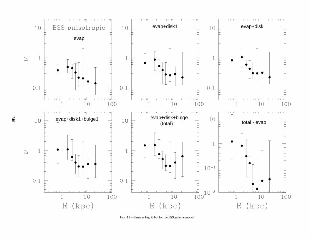
evap

evap+disk1 evap+disk

evap+disk1+bulge1(total)

evap+disk+bulgetotal - evap

FIG. 11.ÈSame as but for the galactic modelFig. 9, BSS

240

evap disk1 disk2

bulge1 bulge2 disk2+bulge2

FIG. 12.ÈDi†erential destruction rate for di†erent processes : evaporation, disk shock with and without induced relaxation (““ disk 1 ÏÏ and ““ disk ÏÏ, respectively), and bulge shock with and withoutrelaxation term (““ bulge 1 ÏÏ and ““ bulge ÏÏ). See text for the deÐnition of the di†erential rate. The error bars indicate the interquartile range of the distribution. Weinberg adiabatic corrections are used.Galactic model is and kinematic model is isotropic.OC,

241

evap disk1 disk2

bulge1 bulge2 disk2+bulge2

FIG. 13.ÈSame as but for the anisotropic kinematic modelFig. 12,

242

evap disk1 disk2

bulge1 bulge2 disk2+bulge2

FIG. 14.ÈSame as but for the galactic modelFig. 12, BSS

243

evap disk1 disk2

bulge1 bulge2 disk2+bulge2

FIG. 15.ÈSame as but for the galactic modelFig. 13, BSS

244

evap evap+disk1 evap+disk

evap+disk1+bulge1(total)

evap+disk+bulge

total - evap

FIG. 16.ÈHistogram distribution of the destruction rates from Weinberg adiabatic correction is used. Galactic model is and kinematic model is isotropic.Fig. 8. OC,

245

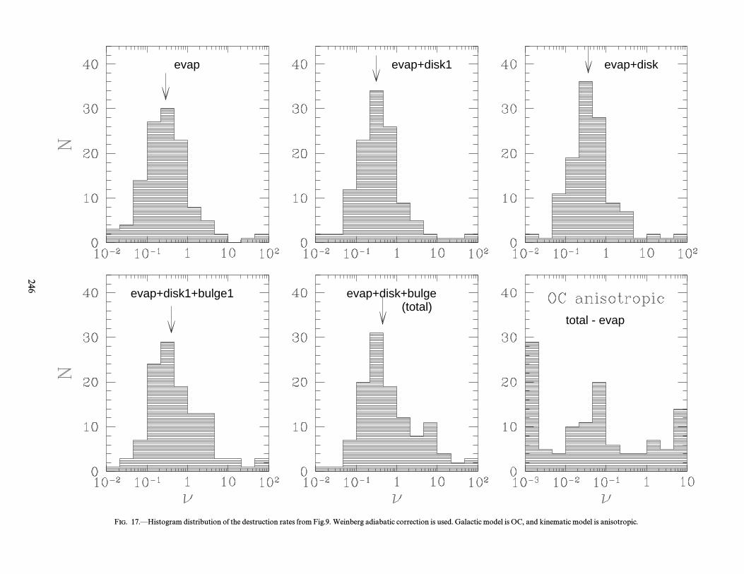
evap evap+disk1 evap+disk

evap+disk1+bulge1(total)

evap+disk+bulge

total - evap

FIG. 17.ÈHistogram distribution of the destruction rates from Weinberg adiabatic correction is used. Galactic model is and kinematic model is anisotropic.Fig.9. OC,

246

evap evap+disk1 evap+disk

evap+disk1+bulge1(total)

evap+disk+bulge

total - evap

FIG. 18.ÈHistogram distribution of the destruction rates from Weinberg adiabatic correction is used. Galactic model is and kinematic model is isotropic.Fig. 10. BSS,

247

evap evap+disk1 evap+disk

evap+disk1+bulge1(total)

evap+disk+bulge

total - evap

FIG. 19.ÈHistogram distribution of the destruction rates from Weinberg adiabatic correction is used. Galactic model is and kinematic model is anisotropic.Fig. 11. BSS,

GALACTIC GLOBULAR CLUSTER SYSTEM 249

FIG. 20.ÈComparison of the calculated tidal radii of the globular clusters with the observed values. The calculated radii are obtained with the formula intext, The left-hand panel shows the original sample used in the Fokker-Planck calculations. Circles mark the core collapse clusters for whicheq. (26).observational determination of tidal radius is less certain. The dotted lines outline the 30% deviation from the observations. The right-hand panel shows thesample obtained from 20 random sample realizations chosen to match the observed R

t.

metry is that the clusters pass close to the Galactic centersometime in their history and experience a very strong tidalÐeld. On the other hand, we expect the clusters to expand alittle after a strong tidal perturbation (see et al.Gnedin

for a detailed discussion and simulations). Therefore,1997bthe orbits that have small perigalacticon would not be nec-essarily inconsistent with a somewhat larger tidal radius,which is now observed. Nevertheless, it is very important toinvestigate the vulnerability of the inferred destruction rateson the initial conditions applied to the clusters.

We have constructed 20 di†erent initial velocity pairsconsistent with the chosen kinematic model. For the sake ofsimplicity, we considered only the isotropic model. ForOCall the initial conditions, we integrated the cluster orbits for1010 yr and calculated the tidal radii from the median peri-galactic distances, as described in Then, the initial° 2.4.velocities that give the best agreement with the observed R

tfor each cluster were combined into one sample. The agree-ment of the tidal radii of the Ðnal sample with the observ-ations is fairly good, with 96 of the total 119 clusters having

within 30% of shows the comparison ofRt

Rt,obs. Figure 20

the observed and inferred tidal radii for the original and theselected samples.

The Fokker-Planck calculations are repeated for the newsample. The median destruction rate is 0.405, with theerrors given in As a further check, we have selectedTable 5.subsamples of clusters that have their initial tidal radiiwithin 50%, 20%, and 5% within the observed values. Forall these subsamples, the median is the same as for thewhole sample, which gives a robust lower limit to thedestruction rate.

The new value of the destruction rate is 22% less thanquoted in The direction of the change is explainedTable 4.by the smaller tidal radii in the original sample. The tidalÐeld on the clusters is stronger, and they are easier todestroy. It is encouraging, however, that the original resultis within twice the error of the new median. To summarize,

we expect the median destruction rates to go down onaverage if we were to use the corrected initial velocities, butthe magnitude of the change is small and no conclusionsmade in would change.° 5

3.3.1. Systematic Error in Median Destruction Rate

To evaluate the systematic error in determination of themedian destruction rate, we ran the Fokker-Planck code forsome of the 20 orbital realizations of the sample with di†er-ent initial velocities. Again, we use the galactic modelOCand the isotropic kinematic model. Each particular realiza-tion is statistically independent of the others, and the set ofsuch calculations provide a quantitative measure of thedependence of the Ðnal results on the initial conditions.

The median rates for these test calculations are given inNaturally, the original sample and the one selectedTable 5.

TABLE 5

DESTRUCTION RATES FOR THE ISOTROPIC MODEL WITHOCDIFFERENT INITIAL CONDITIONS

ltotal Notes

0.518~0.039`0.108 . . . . . . Original result fromTable 40.405~0.068`0.068 . . . . . . Selected orbits to match the observed Rtid0.621~0.057`0.033 . . . . . .0.523~0.050`0.092 . . . . . .0.523~0.122`0.092 . . . . . .0.615~0.124`0.075 . . . . . .0.613~0.124`0.023 . . . . . .0.619~0.089`0.023 . . . . . .0.615~0.142`0.064 . . . . . .0.525~0.073`0.094 . . . . . .0.544~0.088`0.089 . . . . . .0.617~0.083`0.122 . . . . . .0.595~0.099`0.123 . . . . . .

0.56^0.07 . . . . . . . Mean of the set

R<3 kpc

R<5 kpc

R<8 kpc

R<12 kpc

R<3 kpc

R<5 kpc

R<8 kpc

R<12 kpc

R<5 kpc

R<8 kpc

R<12 kpc

R<5 kpc

R<8 kpc

R<12 kpc

250 GNEDIN & OSTRIKER Vol. 474

FIG. 21.ÈVital diagram for the Galactic globular clusters. Mass-radiusplane is restricted by three destructing processes : relaxation, tidal shocks,and dynamical friction. Galactic model is and the kinematic model isOC,isotropic.

to match the observed tidal radii constitute the Ðrst twoentries of the set. None of the new rates is smaller than theoriginal destruction rate of 0.518. The mean of this set is0.56^ 0.07 and is consistent with the original result withinerrors.

A proper determination of the destruction rates wouldrequire careful and thorough selection of the cluster orbitsconsistent with all the known parameters of the globularclusters. It is an important, though computationally inten-sive, step and should be done in the future. The initial con-ditions used in this work did not perfectly agree with theobservations, but the performed tests show reasonable

FIG. 22.ÈSame as but for the anisotropic kinematic modelFig. 21,

FIG. 23.ÈSame as but for the galactic modelFig. 21, BSS

robustness of the results. The use of median of the sampleproved to give a good and reliable measure of the destruc-tion rates.

3.4. V ital Diagram for Globular ClustersWe do not know what was the initial distribution of

globular clusters in our Galaxy. But we can imagine thatthey occupied some volume in a given parameter space. Allthe physical mechanisms considered above tend to destroyclusters with time and thus to reduce the allowed volume.They superimpose particular boundaries that distinguishthe present-day clusters from those being already dissolved(or that were never formed). & Rees consideredFall (1977)the cluster mass versus their typical size (half-mass radius

diagram. The authors included evaporation, disk shock,Rh)

FIG. 24.ÈSame as but for the galactic modelFig. 22, BSS

No. 1, 1997 GALACTIC GLOBULAR CLUSTER SYSTEM 251

and tidal shock heating (for the latter, they assume the tidalinteraction with the clusters themselves rather than with thebulge). These processes cut a triangle on the plane,R

h-M

containing the observed clusters pretty well. J. P. Ostriker(1975, unpublished) and & Castellani alsoCaputo (1984)included dynamical friction, which excludes the verymassive clusters. They noted also that the strength of thedestruction mechanisms varies with galactocentric radius,and therefore the allowed space depends on the position ofa cluster.

We constructed such a vital diagram for the GalacticGCS using our sample and results of the computations of itsevolution. All of the processes used in the simulations, aswell as the dynamical friction, participate in the diagram.The vital boundary is deÐned in such a way that the sum ofall the destruction rates is equal to the inverse Hubble time :

1tHubble

\ 1tev

] 1tsh

] 1tdf

, (31)

where and are the timescales over which a clustertev, tsh, tdfwould be destroyed by the given process alone, for theevaporation, disk and bulge shock combined, and dynami-cal friction, respectively. Note that throughout this paper,we adopted for simplicity yr.tHubble\ 1010

According to the calculations reported in ° 3.1,

tevD 30trh , (32)

where is the half-mass relaxation time We plantrh (eq. [5]).to perform a similar comprehensive analysis for the gravita-tional shocks. At present, we use

tsh\ 1ldisk] lbulge

. (33)

Thus, the shock boundary should be considered as a strong-er limit. We have not considered the e†ects of dynamicalfriction in detail in this paper. & Tremaine (1987, p.Binney

estimated the time for a cluster to lose its momentum428)and fall to the Galactic center (their eq. [7-26]) :

tdf\2.64] 1011 yr

ln "A R

i2 kpc

B2A Vc

250 km s~1BA106 M

_M

B,

(34)

where ln " is the Coulomb logarithm, is the initial galac-Ritocentric distance, is the cluster circular speed, and M isV

cits mass.The cluster vital diagram for the galactic model isOC

shown in Figures and21 22.The diagram for the model is in Figures andBSS 23 24.One can see a signiÐcant fraction of the clusters outside

the ““ surviving ÏÏ boundary. If our picture of the relevantphysical processes is right, they represent a population oflucky Nevertheless, they will be destroyedsurvivors.4within the next Hubble time.

4. DISCUSSION

Using the Fokker-Planck simulations and the sample ofglobular clusters, we estimated a current destruction rateper Hubble time. These results are applicable for thepresent-day clusters evolving forward in time for the nextHubble time. On the other hand, it is of prime interest to

4 We thank the referee for introducing this term.

extract any possible information regarding the past evolu-tion of the clusters from the time of their formation up tonow. We try to construct a simple model for the initialdistribution of the clusters and to test it against the currentdestruction rate. We try then to answer the question raisedin the Introduction : How many of the globular clusters mayhave been destroyed in the history of our Galaxy?

We will not attempt to propose a mechanism for theformation of globular clusters. An example of a possibleformation scenario is given by & Rees Instead,Fall (1985).we assume a lifetime function for the globular clusters, freeof any particular assumptions. Let be a time remainingt

d(t)

to the total destruction of a given cluster at epoch t. Wethen deÐne to be the number of clusters with thef (t

d; t)dt

ddestruction time in the interval at time t. Thus,[td, t

d] dt

d]

if we treat almost all clusters as made in a short time inter-val at the formation of the Galaxy (an obviously grossoversimpliÐcation), then gives the initial distribu-f (t

d; 0)dt

dtion of cluster lifetimes. The normalization is

N(t) \P0

=f (t

d; t)dt

d, (35)

where N(t) is the number of clusters at epoch t. We wouldlike to advance our function f in time starting from theirformation, again without a detailed prescription for theevolution of the cluster sample. We simply assume that allthe clusters were formed at the same time, and that this time

is very small compare to the present Hubble time.t0B 0The number of clusters surviving at the time t is just thenumber of initial clusters with Thus, we have thet

d[ t.

following relation :

f (td; t) \ f (t

d] t ; t0) , (36)

where we have neglected the contribution of in thet0> tÐrst argument of the function f. We call thef (t

d; t0)4 f

i(td)

initial distribution of the globular clusters. Integrated overall destruction times it gives the initial number of globu-t

d,

lar clusters formed in our Galaxy.N(t \ t0) 4 NiWe also deÐne mean and median destruction timest6d

tmaccording to

t6d(t)\ /0= t

df (t

d; t)dt

d/0= f (t

d; t)dt

d\ /0= t

d(td; t)dt

dN(t)

, (37)

12

\ /0tm f (td; t)dt

d/0= f (t

d; t)dt

d\ /0tm f (t

d; t)dt

dN(t)

. (38)

Now we choose two functional forms for which wefi(td),

test against the distribution of the destruction ratesobtained in The simplest one is that with a constant° 3.mean destruction time for all clusters. It assumes an expo-nential form

fi1(td) \ C1 e~atd . (39)

It is easy to show that the mean and median for this dis-tribution are

t6d1 \ 1

a, (40)

tm1 \ ln 2

a. (41)

Thus, the mean destruction rate does not depend on time,and the evaporation of the clusters in this case is similar to

252 GNEDIN & OSTRIKER Vol. 474

radioactive decay. Given the current vital rate, we canalways calculate how many clusters survived from thebeginning. N(t) goes exponentially to zero,

N1(t)\C1a

e~at . (42)

The other function f we consider is a scale-free power law

fi2(td)\ C2 t

d~q . (43)

This distribution is not strictly normalizable since the totalnumber of clusters diverges as approaches zeroN

it0

N2(t)\C2

q [ 1t1~q , q [ 1 . (44)

However, we can successfully apply it to the present time.The corresponding mean and median are

t6d2(t)\

tq [ 2

, q [ 2 , (45)

tm2(t)\ t(21@(q~1) [ 1) . (46)

Note that both these quantities are proportional to the timeof observation. Thus, it seems impossible to determine theinitial cluster population for this distribution, given thecurrent rate. Fortunately, we can compare the shape ofthe distribution with the current proÐle to choose betweenthe two distributions. In addition, we note a very importantdi†erence consequent to the two hypothesized forms for theinitial distribution. In the second (power-law) case, weshould expect that whenever we look, the time tot6

dD t ;

destruction for the clusters that remain is of the same order

as the age of the existing sample. In the Ðrst case, this mightoccur, but it would require a coincidence between the initialtypical time to destruction and the later point in time whenan observer examines the system. T he most important pointto be made in this paper is that the numbers in the last line ofT able 4 are of order unity. This is consistent with the power-law assumption and allows the possibility of large fractionaldestruction.

On we plot a histogram of the destructionFigure 25,rates for our sample of 119 clusters for the galacticOCmodel. The dotted region gives the number of clusters perlogarithmic bin in Two panels correspond to the resultst

d.

obtained with the Weinberg adiabatic correction for theisotropic and anisotropic kinematic models, respectively.We use the medians for the two cases to determine theshape of the two models for the destruction rates. Thedashed curve corresponds to the exponential model, and thesolid line is for the power-law one. Both lines are normal-ized to the present number of clusters, N(tHubble).shows the distribution for the galacticFigure 26 BSSmodel.

We see from this plot that both models are consistentwith the actual distribution. However, in our view, thepower-law case better represents the overall extended shapeof the histogram. The exponential model is more concen-trated around the median value and falls o† very rapidly forlarge It also predicts a much larger number of clusters int

d.

the center of the diagram than follows from the calculations.Therefore, we favor the second choice, namely, the power-law distribution of the destruction times. Based on theresults obtained for the galactic model and WeinbergOCadiabatic correction, the power-law index is q B 1.59È1.64(two limits are for the anisotropic and isotropic kinematicdistributions, respectively). For the model, we ÐndBSS

FIG. 25.ÈDistribution of the destruction times for our sample for the galactic model and Weinberg adiabatic corrections. All destruction processesOCare included. Solid line : power-law distribution, normalized to the present time ; dashes : normalized exponential model.

No. 1, 1997 GALACTIC GLOBULAR CLUSTER SYSTEM 253

FIG. 26.ÈSame as but for the galactic modelFig. 25, BSS

q B 1.73È1.82. Thus, we conclude that the power-law modelwith q \ 1.6È1.8 gives naturally the present distribution ofthe globular cluster destruction times.

From the last sentence it immediately follows that theinitial cluster population could have been much larger thanthe present one. The present-day characteristics do notprovide a deÐnite number, though they do prefer this sce-nario. Thus, it is quite possible that a very signiÐcant frac-tion of the original globular clusters have been alreadydestroyed. Their remnants might now constitute the innerspherical stellar component of our Galaxy, i.e., the bulge.We note also from Figures and that clusters close to8 10the Galactic center are most heavily attacked by the bulgeshock, and therefore most of the dissolved clusters could bein the very central region of the Galaxy. A strong bulgecomponent present in the Ostriker & Caldwell galacticmodel could be enhanced by the input from the destroyedclusters. Note that we do not require the existence of thebulge from the Ðrst days of the Galactic history in order todestroy the clusters. As follows from the power-law dis-tribution, most of the initially formed clusters had relativelyshort lifetimes and presumably were not very massive. Thus,the main mechanism driving their dissolution could havebeen internal relaxation, although, if present in some form,the central Galactic component would be very efficient inthe cluster destruction. In any case, the overall potential ofthe Galaxy is changed only very slightly if we were toimagine that all bulge and spheroid stars were put back intoglobular clusters with appropriate orbits. Thus, even thebulge shock and tidal evaporation processes would beessentially unchanged, if we were to put all stars in thequasi-spherical distribution back into clusters.

Observational data on stellar populations indicate thatthe spheroid of the Galaxy is kinematically and chemicallydistinct from the disk & Ryan Halo stars are(Norris 1991).

old (with ages slightly exceeding our adopted Hubble timeof 1010 yr) and metal poor. Because the density of the proto-galactic gas cloud is not high enough to form stars effi-ciently, the oldest stars in the Galaxy are likely to have beenformed in clusters perhaps not too di†erent from thepresent population of globular clusters. Now we see most ofthe metal-poor stars in the halo, which suggests that most ofthem could be left over from the disrupted clusters. Harris

proposed two arguments against this idea : (1) orbits(1991)of the present globular clusters are more isotropically dis-tributed than those of spheroid stars, and (2) the clustershave systematically lower metallicity than the Ðeld stars andbecome more metal poor with increasing galactocentric dis-tance R. But and & Goodman pointed outAHO Lee (1995)a possible solution for the former problem. The Ðrst of thesearguments can be moderated if we consider the initialcluster distribution. argued that the kinematic modelAHObetter describing the current population is the anisotropicone (see with the orbits getting more and more radial° 2.3)as R increases. The destruction mechanisms are the strong-est in the central few kiloparsecs, especially the bulge shock.Thus, the clusters in the most elongated orbits with smallperigalactic distance would be destroyed Ðrst. Their rem-R

pnants would populate the spheroid as we see it now, withthe preferentially radial orbits of stars. Surviving clusters,on the other hand, have more isotropic orbits consistentwith the observations.

To resolve the problem of metallicities, we refer to vanden Bergh who found that [Fe/H] correlates some-(1995),what more strongly with perigalacticon than with theirR

pcurrent position R. Thus, the metal-rich clusters withsmaller which would be destroyed Ðrst, would enrichR

p,

the halo stellar population. Another solution comes fromthe observed age di†erence in the cluster population. Theformation period could have been extended up to 2È5 Gyr

254 GNEDIN & OSTRIKER Vol. 474

(see references in & Ryan Thus, the very ÐrstNorris 1991).low-mass clusters could dissolve owing to internal relax-ation, but their stars would enrich the primordial gas for thenext generation of clusters. Our power-law hypothesis forthe distribution of the clusters predicts that the mean (andmedian) destruction time is proportional to the time elapsedsince the formation, so that newly formed clusters would beagain most susceptible to disruption. If they were destroyedwithin the remaining 8È10 Gyr, their stars are the Popu-lation II halo stars that we see in our Galaxy.

5. CONCLUSIONS

We have used the Fokker-Planck code to investigate thedestruction rate of globular clusters in our Galaxy. Weapplied two forms of the adiabatic correction for gravita-tional shocks and found that the median results do notdepend much on the particular form of the correction. Thecurrent destruction rate for the sample is about 0.5È0.9 per1010 yr (depending on the Galactic and kinematic models),which implies that more than half of the present clusters areto be destroyed within the next Hubble time. This estimateis approximately a factor of 10 higher than that obtained by

There are two principal reasons for the change. First,AHO.our Fokker-Planck detailed calculations for each clustergive systematically larger rates of two-body relaxation andcore collapse than did the essentially timescale arguments of

Second, the new tidal shock relaxation processAHO.described by further reduces lifetimes by a signiÐcantKOamount.

Trying to understand the original population of Galacticglobular clusters, we considered two possible models for thedistribution of the cluster lifetimes. Both of them can benormalized to the median present destruction rate. Wefavor the power-law model on a basis of shape of the dis-tribution of destruction rates as it naturally explains the factthat the current median time to destruction is comparableto the present mean cluster age and also because the pre-dicted distribution of cluster destruction times provides areasonable match to observations. The power-law distribu-tion allows a much larger number of the clusters to have

been formed initially than is currently observed and allowsthe possibility that the debris of the early disrupted clustersmight have formed much of spheroid of our Galaxy.

has investigated the possibility of popu-Surdin (1995)lating the stellar halo by remnants of the destroyed starcluster (open and globular). He comes to the conclusionthat a much larger number of low-mass (103È104 clus-M

_)

ters than observed now is required to match the mass of thespheroid. This conforms to our result, since low-mass (andhence, weakly concentrated) clusters have short lifetimes.All those nonobserved clusters have to be destroyed beforethe present time.

Finally, we note that the inclusion of the mass spectrumin the Fokker-Planck models would strongly enhance therelaxation and core collapse and would ultimately speed upthe dissolution of the clusters. This could also increase thedestruction rate by a signiÐcant amount.

The destruction rates for the individual clusters are avail-able electronically upon request.

We are greatly indebted to Hyung Mok Lee, who provid-ed us with his Fokker-Planck code. We thank Luis Aguilarfor sharing the orbit integration routine used by AHO.Many people contributed to the compilation of radialvelocities for our sample. George Djorgovski has been aninvaluable source of data tables and references. We aregrateful to Taft Armandro†, Kyle Cudworth, Chris Kocha-nek, and Ruth Peterson for their data, and to Bruce Carney,Chigurapati Murali, Dave Lathau, and Charles Petersonfor useful references. Konrad Kuijken has provided us withthe vertical gravitational force due to the Galactic disk.Finally, we have beneÐted from the discussions with JeremyGoodman, Lars Hernquist, Tomislav Kundic� , Hyung MokLee, David Spergel, Lyman Spitzer, Scott Tremaine, andMartin Weinberg. Most of the calculations have been doneon the SP2 supercomputer at the Maui High PerformanceComputing Center, which we gratefully acknowledge. Wewould like to thank the referee, David Cherno†, for criticalcomments that greatly improved the paper. This work wassupported in part by NSF grant AST 94-24416.

REFERENCESL., Hut, P., & Ostriker, J. P. 1988, ApJ, 335,Aguilar, 720L. A., & White, S. D. M. 1985, ApJ, 295,Aguilar, 374

V. A. 1938, Uch. Zap. L. G. U., 22, 19 ; English transl. inAmbartsumian,IAU Symp. 113, Dynamics of Star Clusters, ed. J. Goodman & P. Hut(Dordrecht : Reidel), 521

T. E., & Da Costa, G. S. 1991, AJ, 101,Armandro†, 1329J. N., Schmidt, M., & Soneira, R. M. 1983, ApJ, 265,Bahcall, 730J., & Tremaine, S. 1987, Galactic Dynamics (Princeton : PrincetonBinney,

Univ. Press)R. D. 1993, poster paper presented at The Globular ClusterÈCannon,

Galaxy Connection Workshop, ASP Conf. Ser., vol. 48, ed. G. H. Smith,& J. P. Brodie (San Francisco : ASP), cited by Costa & Armandro†Da(1995)

F., & Castellani, V. 1984, MNRAS, 207,Caputo, 185D. F., Kochanek, C. S., & Shapiro, S. L. 1986, ApJ, 309,Cherno†, 183D. F., & Shapiro, S. L. 1987, ApJ, 322,Cherno†, 113D. F., & Weinberg, M. D. 1990, ApJ, 351,Cherno†, 121

H. N. 1979, ApJ, 234,Cohn, 10361980, ApJ, 242,ÈÈÈ. 7651985, in IAU Symp. 113, Dynamics of Star Clusters, ed.ÈÈÈ.

J. Goodman & P. Hut (Dordrecht : Reidel), 161K. M., & Hanson, R. B. 1993, AJ, 105,Cudworth, 168

Costa, G. S., & Armandro†, T. E. 1995, AJ, 109,Da 2533Costa, G. S., Armandro†, T. E., & Norris, J. E. 1992, AJ, 104,Da 154

S. 1993, in ASP Conf. Proc. 50, Structure and Dynamics ofDjorgovski,Globular Clusters, ed. S. G. Djorgovski & G. Meylan (San Francisco :ASP), 325

S., & Meylan, G. 1993, in ASP Conf. Proc. 50, Structure andDjorgovski,Dynamics of Globular Clusters, ed. S. G. Djorgovski & G. Meylan (SanFrancisco : ASP), 373

S. M., & Rees, M. J. 1977, MNRAS, 181,Fall, 37P1985, ApJ, 298,ÈÈÈ. 18

C. S., & White, S. D. M. 1980, MNRAS, 193,Frenk, 295D., Piatti, A. E., Claria, J. J., & Minniti, D. 1995, AJ, 109,Geisler, 605O. Y., & Hernquist, L. 1997, inGnedin, preparationO. Y., Lee, H. M., & Ostriker, J. P. 1997a, inGnedin, preparationO. Y., Ostriker, J. P., Johnston, K. V., & Hernquist, L. 1997b, inGnedin,

preparationJ. 1993, in ASP Conf. Proc. 50, Structure and Dynamics ofGoodman,

Globular Clusters, ed. S. G. Djorgovski & G. Meylan (San Francisco :ASP), 87

W. E. 1991, ARA&A, 29,Harris, 543M. 1961, Ann. dÏAp., 24,He� non, 369J. E., Shawl, S. J., & Meyer, J. E. 1986, PASP, 98,Hesser, 403

P., & Djorgovski, S. 1992, Nature, 359,Hut, 806K. A., Harris, W. E., & Webbink, R. F. 1983, AJ, 88,Innanen, 338

D. 1993, AJ, 105,Johnstone, 155M. G., Stuart, A., & Ord, J. K. 1987, KendallÏs Advanced TheoryKendall,

of Statistics, Vol. 1 (5th ed. ; New York : Oxford Univ. Press)I. R. 1966, AJ, 71,King, 64

A. S., & McDowell 1985, unpublished, cited by Kulessa, A. S., &Kulessa,Lynden-Bell, D. 1992, MNRAS, 255, 105

T., & Ostriker, J. P. 1995, ApJ, 438,Kundic� , 702H. M., Fahlman, G. G., & Richer, H. B. 1991, ApJ, 366,Lee, 455H. M., & Goodman, J. 1995, ApJ, 443,Lee, 109H. M., & Ostriker, J. P. 1987, ApJ, 322,Lee, 123

K., Ostriker, J. P., & Aguilar, L. 1992, ApJ, 388,Long, 362D., & Binney, J. J. 1981, Galactic Astronomy (2d ed. ; San Fran-Mihalas,

cisco : Freeman)J. E., & Ryan, S. G. 1991, ApJ, 380,Norris, 403

No. 1, 1997 GALACTIC GLOBULAR CLUSTER SYSTEM 255

K. F. 1965, Dynamics of Stellar Systems (Oxford :Ogorodnikov,Pergamon)

J. P. 1985, in IAU Symp. 113, Dynamics of Star Clusters, ed.Ostriker,J. Goodman & P. Hut (Dordrecht : Reidel), 347

J. P., & Caldwell, J. A. 1983, in Kinematics, Dynamics and Struc-Ostriker,ture of the Milky Way, ed. W. L. H. Shuter (Dordrecht : Reidel), 249

J. P., Spitzer, L., Jr., & Chevalier, R. A. 1972, ApJ, 176,Ostriker, L51R. C., & Cudworth, K. M. 1994, ApJ, 420,Peterson, 612R. C., Rees, R. F., & Cudworth, K. M. 1995, ApJ, 443,Peterson, 124R. C., Seitzer, P., & Cudworth, K. M. 1989, ApJ, 347,Peterson, 251

W. H., Teukolsky, S. A., Vetterling, W. T., & Flannery, B. P. 1992,Press,Numerical Recipes in C (2d ed. ; Cambridge : Cambridge Univ. Press)

C., & Meylan, G. 1993, in ASP Conf. Proc. 50, Structure andPryor,Dynamics of Globular Clusters, ed. S. G. Djorgovski & G. Meylan (SanFrancisco : ASP), 357

A. E., Cudworth, K. M., & Majewski, S. R. 1993, in ASP Conf.Schweitzer,Proc. 48, The Globular ClusterÈGalaxy Connection, ed. G. H. Smith &J. P. Brodie (San Francisco : ASP), 113

L., Jr. 1940, MNRAS, 100,Spitzer, 3971958, ApJ, 127,ÈÈÈ. 17

L., Jr. 1987, Dynamical Evolution of Globular Clusters (Princeton :Spitzer,Princeton Univ. Press)

L., Jr., & Chevalier, R. A. 1973, ApJ, 183,Spitzer, 565L., Jr., & Hart, M. H. 1971, ApJ, 164,Spitzer, 399N., Olszewski, E. W., & Stetson, P. B. 1985, AJ, 90,Suntze†, 481

V. G. 1995, Astron. Lett., 21,Surdin, 508P. 1989, MNRAS, 238,Thomas, 1319

S. C., Djorgovski S., & King, I. R. 1993, in ASP Conf. Proc. 50,Trager,Structure and Dynamics of Globular Clusters, ed. S. G. Djorgovski &G. Meylan (San Francisco : ASP), 347

den Bergh, S. 1995, AJ, 110,van 1171R. F. 1981, ApJS, 45,Webbink, 259M. D. 1994a, AJ, 108,Weinberg, 1398

1994b, AJ, 108,ÈÈÈ. 14031994c, AJ, 108,ÈÈÈ. 1414

S. D. M., & Frenk, C. S. 1983, in Kinematics, Dynamics and Struc-White,ture of the Milky Way, ed. W. L. H. Shuter (Dordrecht : Reidel), 343

D., Olszewski, E. W., Schommer, R. A., Peterson, R. C., & Aaron-Zaritsky,son, M. 1989, ApJ, 345, 759

R., & West, M. J. 1984, ApJS, 55,Zinn, 45