Embed Size (px)
DESCRIPTION
Achieve deffered rendering using compute shaders
Citation preview
1 | P a g e
Deferred rendering using Compute shaders
A comparative study using shader model 4.0 and 5.0
Benjamin Golba

2 | P a g e
This thesis is submitted to the Department of Interaction and System Design at Blekinge Institute of Technology in partial fulfillment of the requirements for the Bachelor degree in Computer Science. The thesis is equivalent to 10 weeks of full time studies.
Contact Information:
Author: Benjamin Golba Address: Folkparksvägen 10:17, 372 40 Ronneby E-mail: [email protected] University advisor: Stefan Petersson Department of Software Engineering and Computer Science Address: Soft Center, RONNEBY Phone: +46 457 38 58 15 Department of Interaction and System Design Blekinge Institute of Technology SE - 372 25 RONNEBY Sweden Internet: http://www.bth.se/tek/ais Phone: +46 457 38 58 00 Fax: +46 457 271 25
3 | P a g e
Abstract
Game developers today are putting a lot of effort into their games. Consumers are hard to please
and demand a game which can provide both fun and visual quality. This is why developers aim to
make the most use of what hardware resources are available to them to achieve the best possible
quality of the game.
It is easy to use too many performance demanding techniques in a game, making the game
unplayable. The hard part is to make the game look good without decreasing the performance. This
can be done by using techniques in a smart way to make the graphics as smooth and efficient as they
can be without compromising the visual quality. One of these techniques is deferred rendering.
The latest version of Microsoft’s graphics platform, DirectX 11, comes with several new features. One
of these is the Compute shader which is a feature making it easier to execute general computation
on the graphics card. Developers do not need to use DirectX 11 cards to be able to use this feature
though. Microsoft has made it available on graphic cards made for DirectX 10 as well. There are
however a few differences between the two versions. The focus of this report will be to investigate
the possible performance differences between these versions on when using deferred rendering.
An application was made supporting both shader model 4 and 5 of the compute shader, to be able to
investigate this.
Keywords Deferred rendering, DirectX, Direct3D, Vertex shader, Pixel shader, Compute shader
4 | P a g e
Table of contents
Abstract ................................................................................................................................................... 3
Keywords ............................................................................................................................................. 3
1. Introduction ......................................................................................................................................... 6
1.1 Background ........................................................................................................................................ 6
1.2 Research objectives ........................................................................................................................... 7
1.3 Hypothesis ......................................................................................................................................... 7
1.4 Methodology ..................................................................................................................................... 7
1.5 Delimitations ..................................................................................................................................... 7
1.6 Acknowledgements ........................................................................................................................... 7
2. Programming in three dimensions using Direct3D ............................................................................. 8
2.1 Primitives ........................................................................................................................................... 9
2.2 Resources ........................................................................................................................................ 10
2.2.1 Textures .................................................................................................................................... 10
2.2.2 Buffers ...................................................................................................................................... 11
2.2.3 Unordered Access Views .......................................................................................................... 11
2.3 Programmable shaders ................................................................................................................... 11
2.3.1 Vertex shader ........................................................................................................................... 12
2.3.2 Pixel shader .............................................................................................................................. 12
2.3.3 Compute shader ....................................................................................................................... 12
3. Deferred rendering ............................................................................................................................ 14
3.1 Forward rendering ........................................................................................................................... 14
3.2 Deferred rendering .......................................................................................................................... 14
3.2.1 Multiple Render Targets ........................................................................................................... 15
3.2.2 Filling the G-buffer ................................................................................................................... 15
3.2.3 Rendering lights ........................................................................................................................ 15
4. Prototype performance ..................................................................................................................... 17
4.1 The prototype .................................................................................................................................. 17
4.2 Performance testing ........................................................................................................................ 18
4.2.1 Test 1 ........................................................................................................................................ 19
4.2.2 Test 2 ........................................................................................................................................ 20
5 | P a g e
4.2.3 Test 3 ........................................................................................................................................ 21
4.2.4 Test 4 ........................................................................................................................................ 22
5. Discussion and conclusion ................................................................................................................. 23
5.1 Discussion of test 1 and 2 ................................................................................................................ 23
5.2 Discussion of test 3 and 4 ................................................................................................................ 24
5.3 Discussion ........................................................................................................................................ 25
5.2 Conclusion ....................................................................................................................................... 26
6. References ......................................................................................................................................... 27
6.1 Bibliography ..................................................................................................................................... 27
6.2 Papers .............................................................................................................................................. 27
6.3 Presentations ................................................................................................................................... 27
6.4 Websites .......................................................................................................................................... 27
Apendix A – Compute shader code ....................................................................................................... 28
Apendix B – G-buffer filling code ........................................................................................................... 29
6 | P a g e
1. Introduction
This chapter is an introduction to what this thesis is about and the work I have put into it. I will
mention the background information to the topic as well as the methodology chosen to investigate
the hypothesis. Research objectives and delimitations are also present in this chapter.
1.1 Background Most games that use some kind of graphical interface have a rendering procedure. There are two
rasterization-based rendering methods today: forward rendering and deferred rendering. This report
will focus on deferred rendering using Microsoft DirectX and Compute shaders[15].
Forward rendering, which is the classic approach to rendering scenes, calculates lighting per object. If
one object is affected by three lights, it has to be rendered one time for each light source to
accumulate for each light effect. Deferred rendering however, first renders all of the objects
information to multiple render targets (MRTs), which are also known as G-Buffers[2]. What this
information is differs between each implementation. When the Geometry Buffer (G-buffer) has been
filled, this information is later on merged together on to one output buffer, also called the back
buffer. This will be thoroughly explained in chapter 3.
There are a few drawbacks with both of these techniques though. Where forward rendering scales
badly with complex lighting, deferred rendering has high memory requirements and does not work
very well with transparency and multisampling anti-aliasing (MSAA). There are ways to work around
these issues, but the solutions are rarely as good as forward rendering. Deferred rendering does not
fit all graphics engines, since the benefits that it provides are not necessarily something the game will
benefit from. It is known for being very good to render huge amounts of light sources, as well as
work very well with different shadowing techniques such as ambient occlusion[13] and shadow
mapping[14].
The compute shader has opened a lot of doors when it comes to optimizing deferred rendering
further. As this is a post processing technique, the compute shader is said to have a 50-70%
performance increase on deferred rendering-based graphics engines[1]. According to Steams monthly
hardware survey, approximately 53% of its users have a DirectX 10 graphics card, while only 3.29% of
the users have hardware to support DirectX 11[10]. Many of the popular games today have DirectX 10
support[11], and game companies are slowly starting to support DirectX 11 as well[12]. Based on these
numbers you can say that the compute shader is available to the majority of users. This report will
focus on finding out the differences in performance between deferred shading implemented on
DirectX 10 and DirectX 11 based hardware, using the compute shader.
The results of these performance measurements will be analyzed and presented in this thesis. This
thesis will also contain theory behind the different techniques as well as code examples from the
important parts of the test application.
7 | P a g e
1.2 Research objectives The goal of this thesis is to find out if deferred rendering-based graphics engines using compute
shaders have better performance in DirectX 11 than in DirectX 10. This is done by developing a
simple application using compute shaders from both DirectX versions and measuring their
performance.
1.3 Hypothesis The deferred rendering performance between Compute shaders in DirectX 10 and DirectX 11 is
measurably better in DirectX 11.
This is based on a presentation of the Compute shader in DirectX 11, presented at GameFest 2008[1].
It says that deferred rendering-based engines gain from 50% to 70% performance compared to
forward rendering-based ones. The compute shader in DirectX 10 is somewhat limited though, which
is why I think that DirectX 11 will have better performance when using its compute shader.
1.4 Methodology The approach to finding out whether the hypothesis is going to be correct or not was to develop an
application to investigate the differences between deferred shading implemented with compute
shaders in DirectX 10 and 11.
This application is used to perform tests to be able to obtain the required performance data. These
tests are presented in chapter 5. Based on the test data there are conclusions drawn for each tests.
1.5 Delimitations Chapter 3 covers two render commonly used rendering techniques. These two are forward rendering
and deferred rendering, however the focus will be on deferred rendering and compute shaders.
The test application is implemented using DirectX 10 and 11, where the compute shader is available.
There will be no coverage of other rendering software as well as older versions of DirectX.
The basic knowledge to understand this thesis includes 3D programming and knowledge of
Microsoft’s DirectX API.
1.6 Acknowledgements I would like to show my appreciation to my supervisor, Stefan Petersson, for having a positive and
motivating attitude as well as great knowledge of 3D programming.
8 | P a g e
2. Programming in three dimensions using Direct3D
This chapter is an overview of how to program in three dimensions. The point of it is to make the
reader familiar with how it works and introduce the most basic concepts related to rendering and to
this thesis. The contents of this chapter will only scratch the surface, without go too much in to
detail.
Since DirectX is only a collection of application programming interfaces (APIs), I will from now on
refer to Direct3D which handles all 3D related rendering. The Direct3D of DirectX 10 has a
programmable pipeline (previous versions also had a fixed function pipeline), which means it has
programmable units, also known as shaders. Direct3D also has different resource types, such as
textures and buffers. More information on this will be given in the sections below.
Before we go into specific parts of the pipeline, there are a couple of steps you need to go through
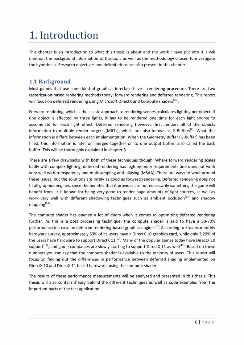
before you can render primitives. Firstly you need to initialize Direct3D. This includes setting up a
Back buffer and a Swap chain. To understand this you can imagine two frames. One of them being
the back buffer currently being displayed on your monitor, and the second one being the buffer to
which Direct3D renders all geometry which will be displayed to you the next frame. These two
buffers are switched between each other thus creating the swap chain[5] [Figure 2.1].
Figure 2.1: Swap chain
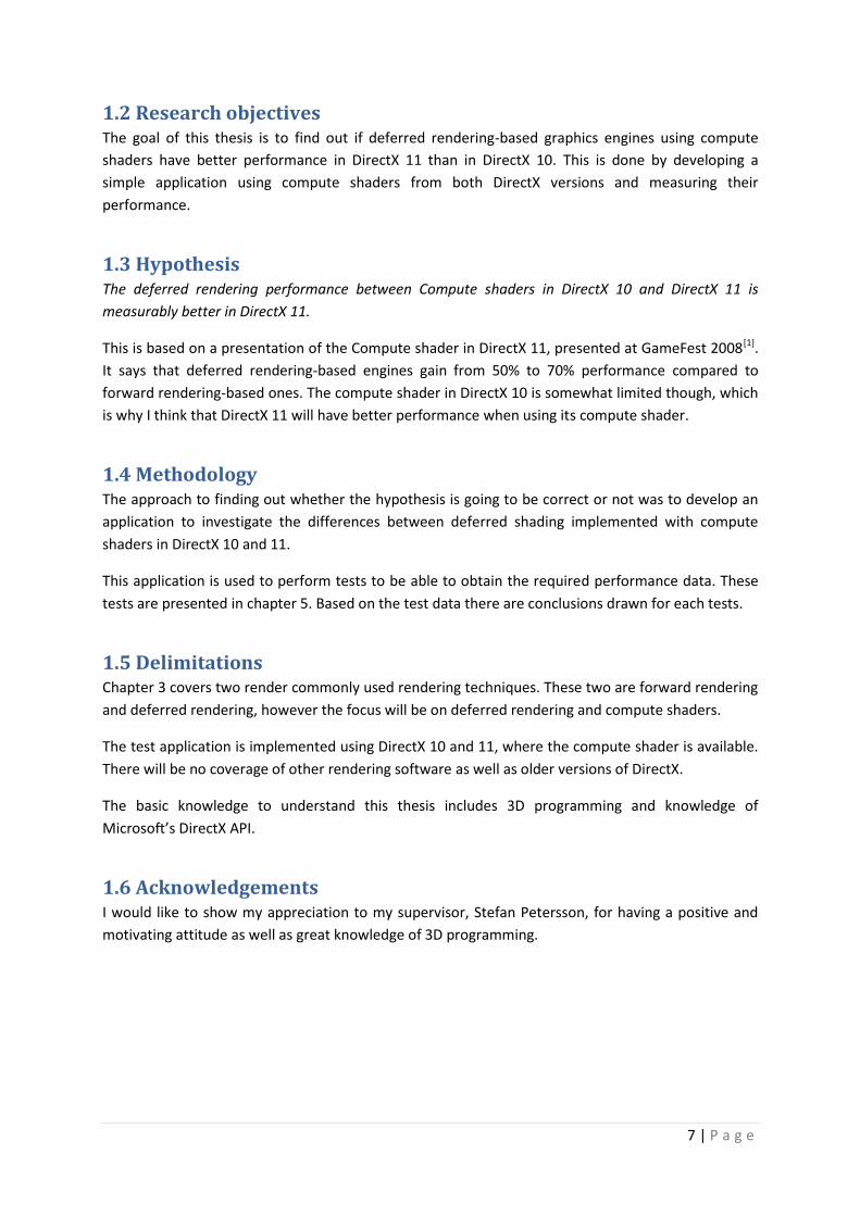
The next important part of the pipeline is the Input assembler (IA). Its job is to take care of the
geometric data that is going to be sent through the vertex shader, and then through the rest of the
shaders defined by the user. Even though Direct3D has no fixed function pipeline, the Input
9 | P a g e
Assembler and the output merger stage (OM), are fixed functions. The OM stage is the last step of
the rendering pipeline. Its job is to merge the results from the pipeline into the final pixels you
eventually see on the screen[6]. Figure 2.2 explains this.
Figure 2.2: Graphics Pipeline
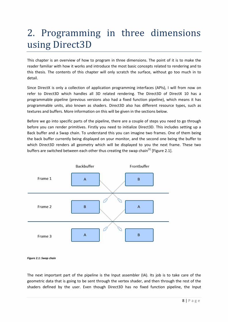
2.1 Primitives Primitives are built up of vertices. A vertex is a data structure that describes a point in space. A
triangle just needs 3 vertices to be complete [Figure 2.2], however a more detailed object can be
built up of several thousands of these [Figure 2.3].
Figure 2.2: Triangle Figure 2.3: Stones on the ground [DirectX 11 SDK, Detail Tessellation sample]
Input Assembler
Vertex shader
Geometry shader
Pixel shader
Output Merger
Final image
10 | P a g e
2.2 Resources Direct3D has two resource types, textures and buffers, which are areas in the memory reserved for
things such as input geometry, shader resources and textures to name a few[7]. These are necessary
in order for the pipeline to access memory efficiently. A resource can be created with many different
options to it. For instance, you can set a texture to have read and write access by either the GPU or
the CPU. There is also a special option, which allows read and write access to both the GPU and CPU,
and is used for data transfers between the two. The most commonly used setting is to only allow the
GPU to read and write to the texture[16]. These options all depend on what you need to do with the
resource, and also if you need speed more than functionality or the other way around. It is a tradeoff
you consider when creating the resource.
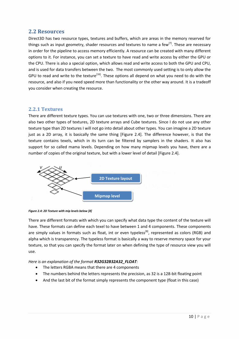
2.2.1 Textures There are different texture types. You can use textures with one, two or three dimensions. There are
also two other types of textures, 2D texture arrays and Cube textures. Since I do not use any other
texture type than 2D textures I will not go into detail about other types. You can imagine a 2D texture
just as a 2D array, it is basically the same thing [Figure 2.4]. The difference however, is that the
texture contains texels, which in its turn can be filtered by samplers in the shaders. It also has
support for so called mama levels. Depending on how many mipmap levels you have, there are a
number of copies of the original texture, but with a lower level of detail [Figure 2.4].
Figure 2.4: 2D Texture with mip levels below [8]
There are different formats with which you can specify what data type the content of the texture will
have. These formats can define each texel to have between 1 and 4 components. These components
are simply values in formats such as float, int or even typeless[8], represented as colors (RGB) and
alpha which is transparency. The typeless format is basically a way to reserve memory space for your
texture, so that you can specify the format later on when defining the type of resource view you will
use.
Here is an explanation of the format R32G32B32A32_FLOAT:
The letters RGBA means that there are 4 components
The numbers behind the letters represents the precision, as 32 is a 128-bit floating point
And the last bit of the format simply represents the component type (float in this case)
2D Texture layout
Mipmap level
11 | P a g e
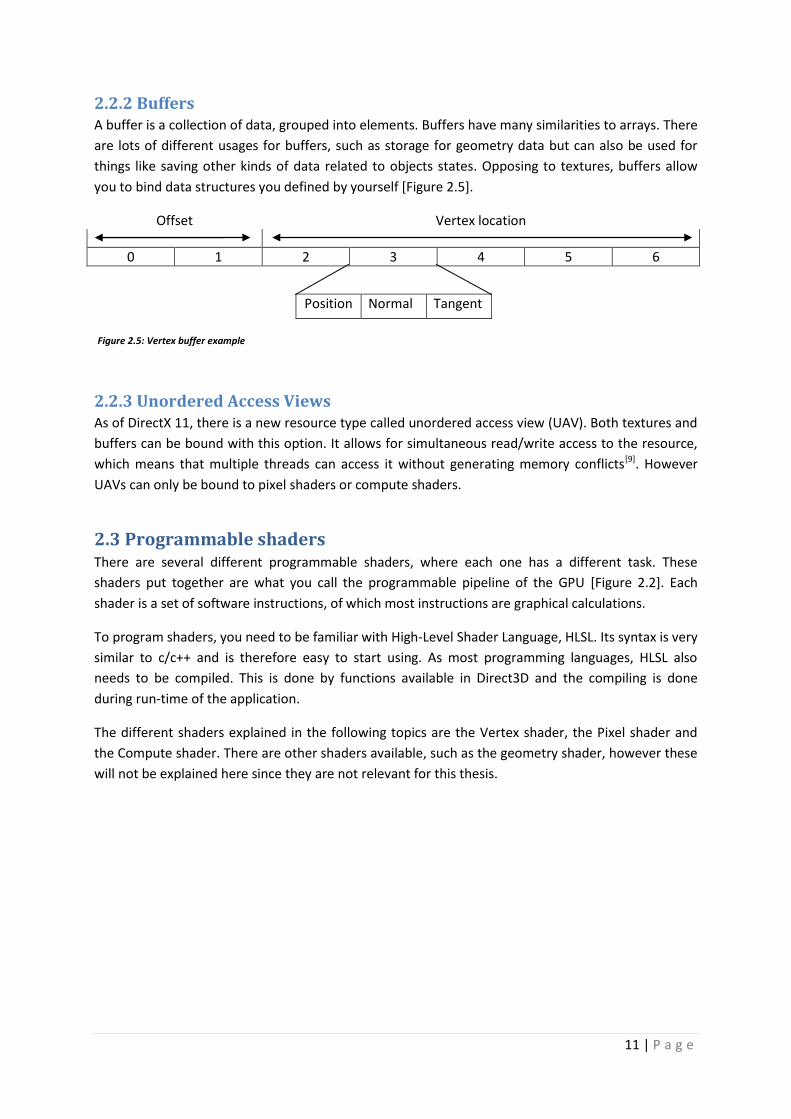
2.2.2 Buffers A buffer is a collection of data, grouped into elements. Buffers have many similarities to arrays. There
are lots of different usages for buffers, such as storage for geometry data but can also be used for
things like saving other kinds of data related to objects states. Opposing to textures, buffers allow
you to bind data structures you defined by yourself [Figure 2.5].
Offset Vertex location
0 1 2 3 4 5 6
Figure 2.5: Vertex buffer example
2.2.3 Unordered Access Views As of DirectX 11, there is a new resource type called unordered access view (UAV). Both textures and
buffers can be bound with this option. It allows for simultaneous read/write access to the resource,
which means that multiple threads can access it without generating memory conflicts[9]. However
UAVs can only be bound to pixel shaders or compute shaders.
2.3 Programmable shaders There are several different programmable shaders, where each one has a different task. These
shaders put together are what you call the programmable pipeline of the GPU [Figure 2.2]. Each
shader is a set of software instructions, of which most instructions are graphical calculations.
To program shaders, you need to be familiar with High-Level Shader Language, HLSL. Its syntax is very
similar to c/c++ and is therefore easy to start using. As most programming languages, HLSL also
needs to be compiled. This is done by functions available in Direct3D and the compiling is done
during run-time of the application.
The different shaders explained in the following topics are the Vertex shader, the Pixel shader and
the Compute shader. There are other shaders available, such as the geometry shader, however these
will not be explained here since they are not relevant for this thesis.
Position Normal Tangent
12 | P a g e
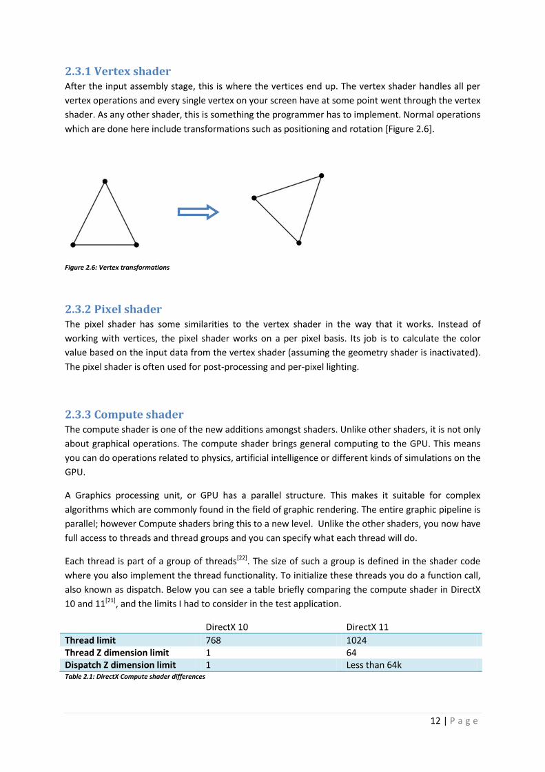
2.3.1 Vertex shader After the input assembly stage, this is where the vertices end up. The vertex shader handles all per
vertex operations and every single vertex on your screen have at some point went through the vertex
shader. As any other shader, this is something the programmer has to implement. Normal operations
which are done here include transformations such as positioning and rotation [Figure 2.6].
Figure 2.6: Vertex transformations
2.3.2 Pixel shader The pixel shader has some similarities to the vertex shader in the way that it works. Instead of
working with vertices, the pixel shader works on a per pixel basis. Its job is to calculate the color
value based on the input data from the vertex shader (assuming the geometry shader is inactivated).
The pixel shader is often used for post-processing and per-pixel lighting.
2.3.3 Compute shader The compute shader is one of the new additions amongst shaders. Unlike other shaders, it is not only
about graphical operations. The compute shader brings general computing to the GPU. This means
you can do operations related to physics, artificial intelligence or different kinds of simulations on the
GPU.
A Graphics processing unit, or GPU has a parallel structure. This makes it suitable for complex
algorithms which are commonly found in the field of graphic rendering. The entire graphic pipeline is
parallel; however Compute shaders bring this to a new level. Unlike the other shaders, you now have
full access to threads and thread groups and you can specify what each thread will do.
Each thread is part of a group of threads[22]. The size of such a group is defined in the shader code
where you also implement the thread functionality. To initialize these threads you do a function call,
also known as dispatch. Below you can see a table briefly comparing the compute shader in DirectX
10 and 11[21], and the limits I had to consider in the test application.
DirectX 10 DirectX 11
Thread limit 768 1024 Thread Z dimension limit 1 64 Dispatch Z dimension limit 1 Less than 64k Table 2.1: DirectX Compute shader differences
13 | P a g e
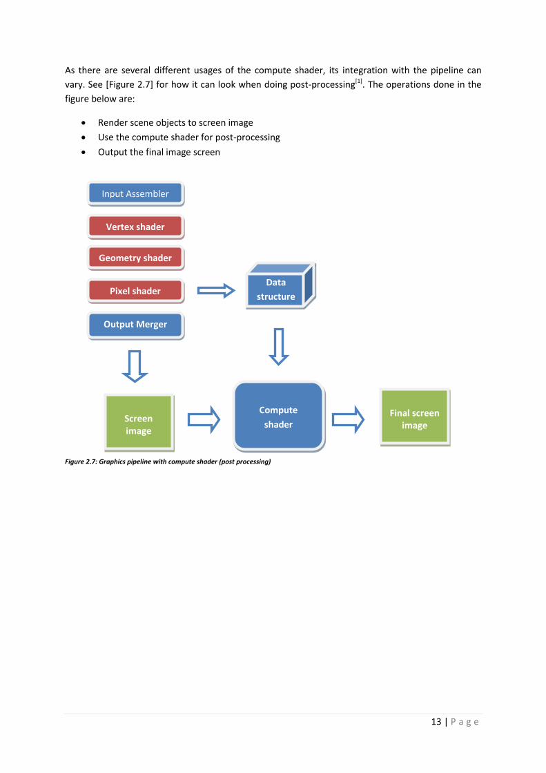
As there are several different usages of the compute shader, its integration with the pipeline can
vary. See [Figure 2.7] for how it can look when doing post-processing[1]. The operations done in the
figure below are:
Render scene objects to screen image
Use the compute shader for post-processing
Output the final image screen
Figure 2.7: Graphics pipeline with compute shader (post processing)
Input Assembler
Vertex shader
Geometry shader
Pixel shader
Output Merger
Screen image
Data
structure
Compute
shader
Final screen
image
14 | P a g e
3. Deferred rendering
The focus of this chapter lies on deferred rendering. However, there will be a brief introduction and
comparison to the classical approach to render 3D scenes, which is also known as forward rendering.
Most 3D scenes in games have a set of objects (houses, guns, cars and so on) which have to be
rendered. To add realism to the game they also have to be lit, and they usually also have additional
techniques added to them, such as different shadowing techniques. Both of these rendering
techniques are commonly used in games today and they both have their own advantages and
disadvantages, which make them especially good for certain types of games, while being less suitable
for other game types.
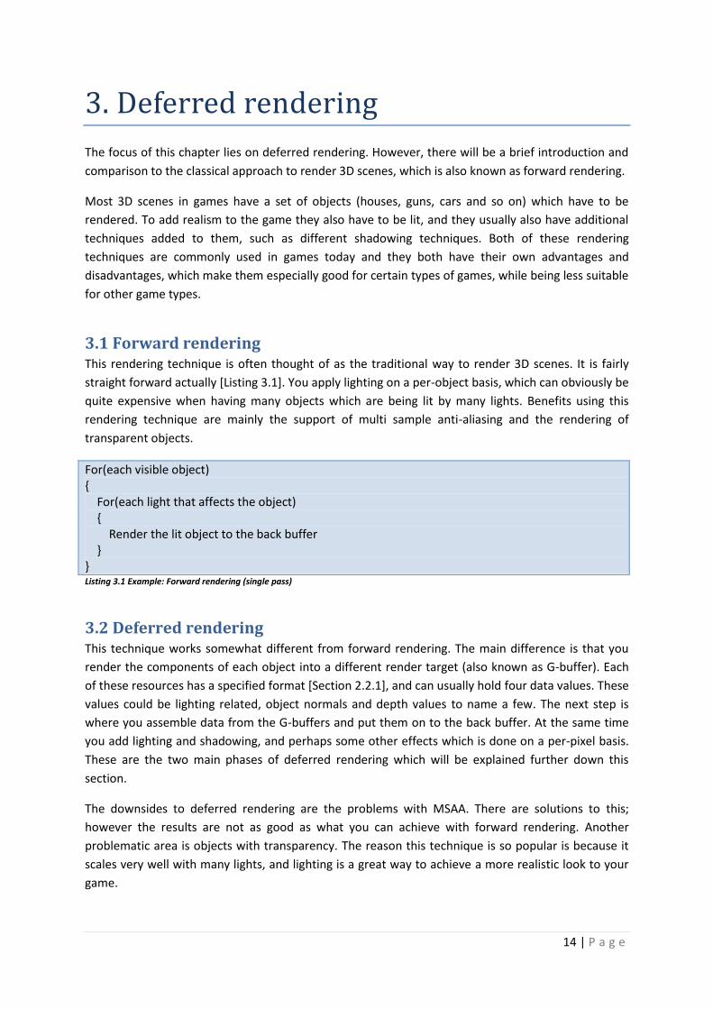
3.1 Forward rendering This rendering technique is often thought of as the traditional way to render 3D scenes. It is fairly
straight forward actually [Listing 3.1]. You apply lighting on a per-object basis, which can obviously be
quite expensive when having many objects which are being lit by many lights. Benefits using this
rendering technique are mainly the support of multi sample anti-aliasing and the rendering of
transparent objects.
For(each visible object) { For(each light that affects the object) { Render the lit object to the back buffer } } Listing 3.1 Example: Forward rendering (single pass)
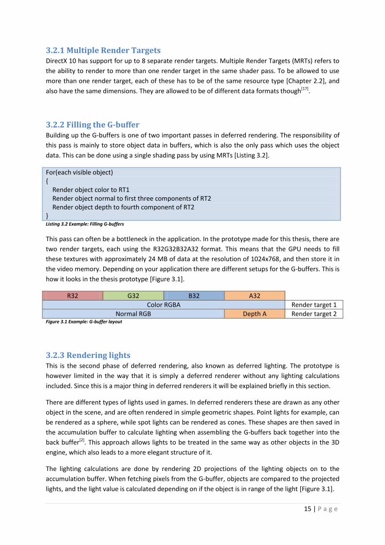
3.2 Deferred rendering This technique works somewhat different from forward rendering. The main difference is that you
render the components of each object into a different render target (also known as G-buffer). Each
of these resources has a specified format [Section 2.2.1], and can usually hold four data values. These
values could be lighting related, object normals and depth values to name a few. The next step is
where you assemble data from the G-buffers and put them on to the back buffer. At the same time
you add lighting and shadowing, and perhaps some other effects which is done on a per-pixel basis.
These are the two main phases of deferred rendering which will be explained further down this
section.
The downsides to deferred rendering are the problems with MSAA. There are solutions to this;
however the results are not as good as what you can achieve with forward rendering. Another
problematic area is objects with transparency. The reason this technique is so popular is because it
scales very well with many lights, and lighting is a great way to achieve a more realistic look to your
game.
15 | P a g e
3.2.1 Multiple Render Targets DirectX 10 has support for up to 8 separate render targets. Multiple Render Targets (MRTs) refers to
the ability to render to more than one render target in the same shader pass. To be allowed to use
more than one render target, each of these has to be of the same resource type [Chapter 2.2], and
also have the same dimensions. They are allowed to be of different data formats though[17].
3.2.2 Filling the G-buffer Building up the G-buffers is one of two important passes in deferred rendering. The responsibility of
this pass is mainly to store object data in buffers, which is also the only pass which uses the object
data. This can be done using a single shading pass by using MRTs [Listing 3.2].
For(each visible object) { Render object color to RT1 Render object normal to first three components of RT2 Render object depth to fourth component of RT2 } Listing 3.2 Example: Filling G-buffers
This pass can often be a bottleneck in the application. In the prototype made for this thesis, there are
two render targets, each using the R32G32B32A32 format. This means that the GPU needs to fill
these textures with approximately 24 MB of data at the resolution of 1024x768, and then store it in
the video memory. Depending on your application there are different setups for the G-buffers. This is
how it looks in the thesis prototype [Figure 3.1].
R32 G32 B32 A32
Color RGBA Render target 1
Normal RGB Depth A Render target 2 Figure 3.1 Example: G-buffer layout
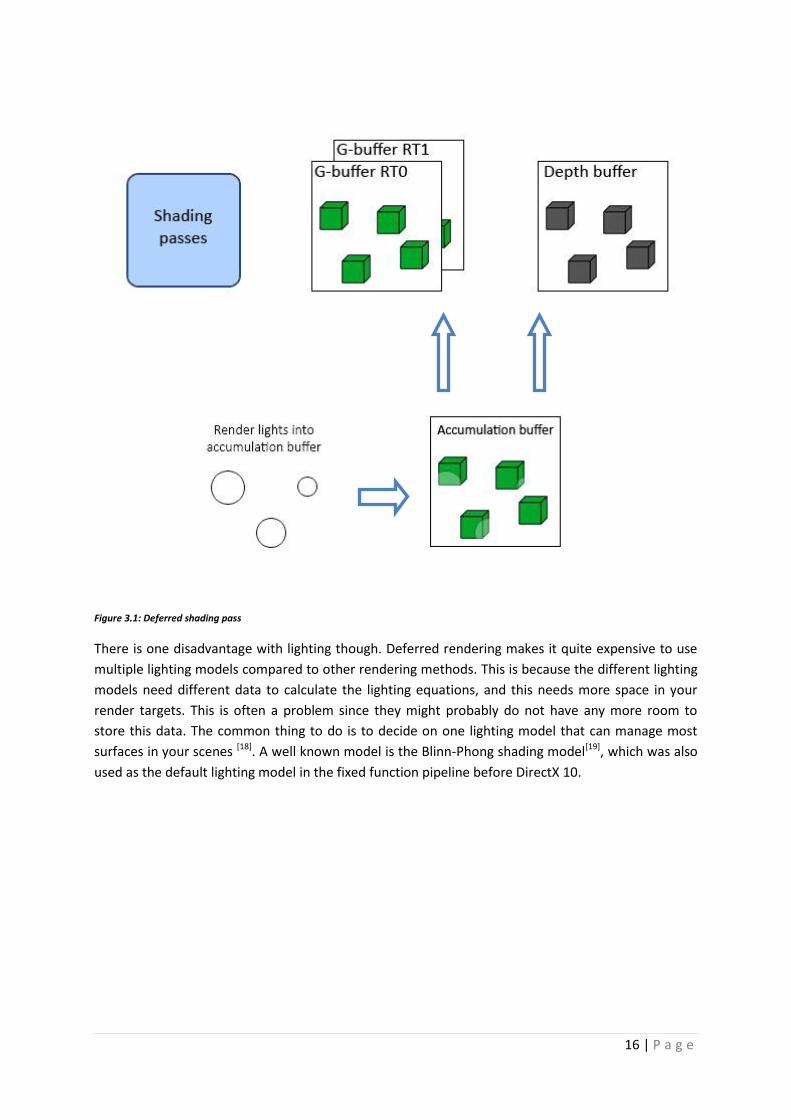
3.2.3 Rendering lights This is the second phase of deferred rendering, also known as deferred lighting. The prototype is
however limited in the way that it is simply a deferred renderer without any lighting calculations
included. Since this is a major thing in deferred renderers it will be explained briefly in this section.
There are different types of lights used in games. In deferred renderers these are drawn as any other
object in the scene, and are often rendered in simple geometric shapes. Point lights for example, can
be rendered as a sphere, while spot lights can be rendered as cones. These shapes are then saved in
the accumulation buffer to calculate lighting when assembling the G-buffers back together into the
back buffer[2]. This approach allows lights to be treated in the same way as other objects in the 3D
engine, which also leads to a more elegant structure of it.
The lighting calculations are done by rendering 2D projections of the lighting objects on to the
accumulation buffer. When fetching pixels from the G-buffer, objects are compared to the projected
lights, and the light value is calculated depending on if the object is in range of the light [Figure 3.1].
16 | P a g e
Figure 3.1: Deferred shading pass
There is one disadvantage with lighting though. Deferred rendering makes it quite expensive to use
multiple lighting models compared to other rendering methods. This is because the different lighting
models need different data to calculate the lighting equations, and this needs more space in your
render targets. This is often a problem since they might probably do not have any more room to
store this data. The common thing to do is to decide on one lighting model that can manage most
surfaces in your scenes [18]. A well known model is the Blinn-Phong shading model[19], which was also
used as the default lighting model in the fixed function pipeline before DirectX 10.

17 | P a g e
4. Prototype performance
The main focus of this chapter is on performance testing. The tests performed are measuring how
deferred rendering differs from being implemented using Compute shaders in DirectX 10 and 11.
4.1 The prototype The test application is developed to test deferred rendering using compute shaders. To test both
shader model 4 and shader model 5, the application supports run-time switching between these two
versions. This is possible by compiling all shaders when loading the application and then using the
selected version by pressing a button.
As mentioned earlier, the goal of this prototype is to test deferred rendering. This means that there
are no lighting or shading calculations performed. The application fills the G-buffers, by rendering
objects and saving their data into MRTs. The next step is to assemble everything into one buffer. This
is done by using the compute shader, which reads from the render targets, and saves the assembled
data into one buffer. This is then rendered to the back buffer.
The performance tests are done by using a timer, starting at the point from where you want to start
measuring and stopping where the frame ends. The measuring of the entire frame is simple. You
start the timer at the beginning of the frame loop and end it at its end. To measure the compute
shader you have to start the timer where the compute shader starts working and end it when it is
finished. The problem here is that the compute shader runs in parallel with the CPU, which means
that the CPU will not wait for the compute shader to finish its calculations before it continues. To
work around this there is something called Queries in Direct3D[20].This is done by creating a query to
the GPU, before your parallel code and then fetching it at the point where the CPU cannot continue
before the shader has finished.
Compute shader 4 has limited thread size. Maximum amount of threads is 768 while compute shader
5 allows up to 1024 threads. To compensate this, there has to be more thread groups dispatched
when running shader model 4 in the application.
18 | P a g e
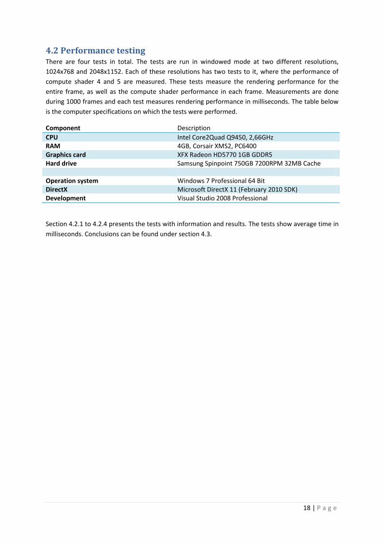
4.2 Performance testing There are four tests in total. The tests are run in windowed mode at two different resolutions,
1024x768 and 2048x1152. Each of these resolutions has two tests to it, where the performance of
compute shader 4 and 5 are measured. These tests measure the rendering performance for the
entire frame, as well as the compute shader performance in each frame. Measurements are done
during 1000 frames and each test measures rendering performance in milliseconds. The table below
is the computer specifications on which the tests were performed.
Component Description
CPU Intel Core2Quad Q9450, 2,66GHz RAM 4GB, Corsair XMS2, PC6400 Graphics card XFX Radeon HD5770 1GB GDDR5 Hard drive Samsung Spinpoint 750GB 7200RPM 32MB Cache Operation system Windows 7 Professional 64 Bit DirectX Microsoft DirectX 11 (February 2010 SDK) Development Visual Studio 2008 Professional
Section 4.2.1 to 4.2.4 presents the tests with information and results. The tests show average time in
milliseconds. Conclusions can be found under section 4.3.
19 | P a g e
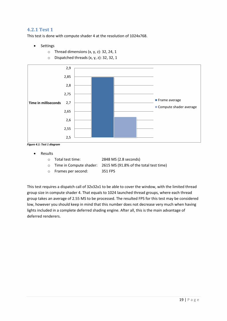
4.2.1 Test 1 This test is done with compute shader 4 at the resolution of 1024x768.
Settings
o Thread dimensions (x, y, z): 32, 24, 1
o Dispatched threads (x, y, z): 32, 32, 1
Figure 4.1: Test 1 diagram
Results
o Total test time: 2848 MS (2.8 seconds)
o Time in Compute shader: 2615 MS (91.8% of the total test time)
o Frames per second: 351 FPS
This test requires a dispatch call of 32x32x1 to be able to cover the window, with the limited thread
group size in compute shader 4. That equals to 1024 launched thread groups, where each thread
group takes an average of 2.55 MS to be processed. The resulted FPS for this test may be considered
low, however you should keep in mind that this number does not decrease very much when having
lights included in a complete deferred shading engine. After all, this is the main advantage of
deferred renderers.
2,5
2,55
2,6
2,65
2,7
2,75
2,8
2,85
2,9
Time in millisecondsFrame average
Compute shader average
20 | P a g e
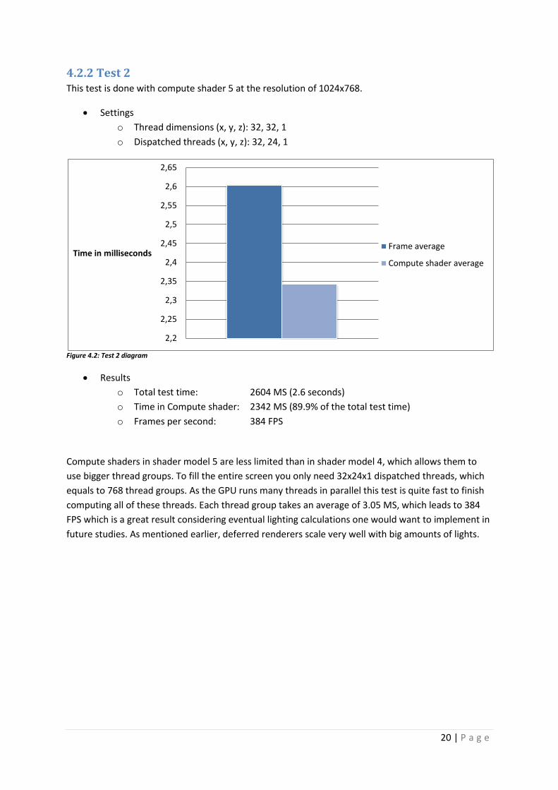
4.2.2 Test 2 This test is done with compute shader 5 at the resolution of 1024x768.
Settings
o Thread dimensions (x, y, z): 32, 32, 1
o Dispatched threads (x, y, z): 32, 24, 1
Figure 4.2: Test 2 diagram
Results
o Total test time: 2604 MS (2.6 seconds)
o Time in Compute shader: 2342 MS (89.9% of the total test time)
o Frames per second: 384 FPS
Compute shaders in shader model 5 are less limited than in shader model 4, which allows them to
use bigger thread groups. To fill the entire screen you only need 32x24x1 dispatched threads, which
equals to 768 thread groups. As the GPU runs many threads in parallel this test is quite fast to finish
computing all of these threads. Each thread group takes an average of 3.05 MS, which leads to 384
FPS which is a great result considering eventual lighting calculations one would want to implement in
future studies. As mentioned earlier, deferred renderers scale very well with big amounts of lights.
2,2
2,25
2,3
2,35
2,4
2,45
2,5
2,55
2,6
2,65
Time in millisecondsFrame average
Compute shader average
21 | P a g e
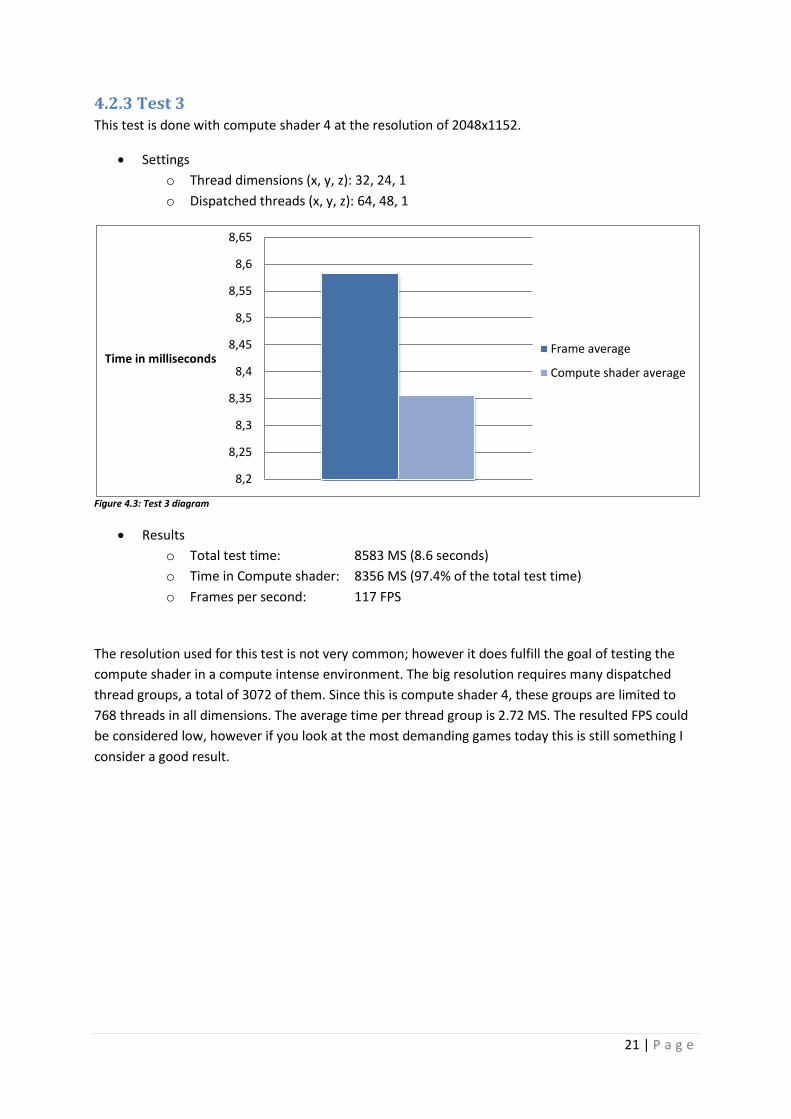
4.2.3 Test 3 This test is done with compute shader 4 at the resolution of 2048x1152.
Settings
o Thread dimensions (x, y, z): 32, 24, 1
o Dispatched threads (x, y, z): 64, 48, 1
Figure 4.3: Test 3 diagram
Results
o Total test time: 8583 MS (8.6 seconds)
o Time in Compute shader: 8356 MS (97.4% of the total test time)
o Frames per second: 117 FPS
The resolution used for this test is not very common; however it does fulfill the goal of testing the
compute shader in a compute intense environment. The big resolution requires many dispatched
thread groups, a total of 3072 of them. Since this is compute shader 4, these groups are limited to
768 threads in all dimensions. The average time per thread group is 2.72 MS. The resulted FPS could
be considered low, however if you look at the most demanding games today this is still something I
consider a good result.
8,2
8,25
8,3
8,35
8,4
8,45
8,5
8,55
8,6
8,65
Time in millisecondsFrame average
Compute shader average
22 | P a g e
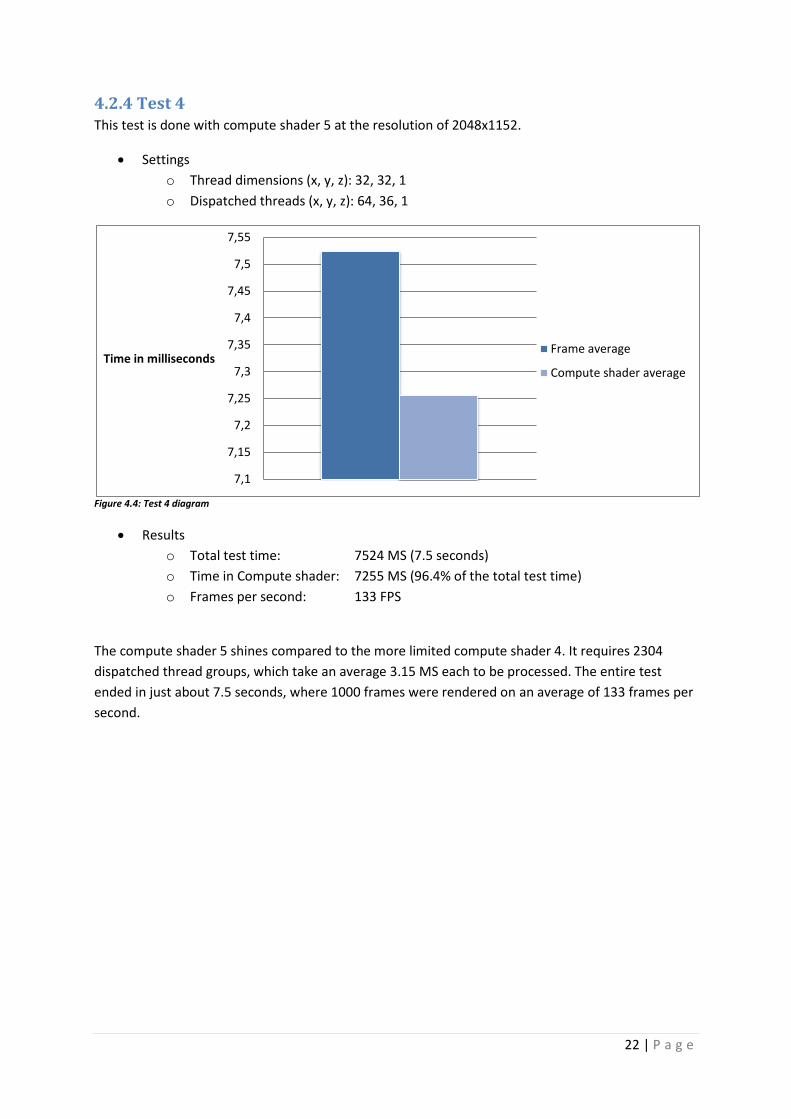
4.2.4 Test 4 This test is done with compute shader 5 at the resolution of 2048x1152.
Settings
o Thread dimensions (x, y, z): 32, 32, 1
o Dispatched threads (x, y, z): 64, 36, 1
Figure 4.4: Test 4 diagram
Results
o Total test time: 7524 MS (7.5 seconds)
o Time in Compute shader: 7255 MS (96.4% of the total test time)
o Frames per second: 133 FPS
The compute shader 5 shines compared to the more limited compute shader 4. It requires 2304
dispatched thread groups, which take an average 3.15 MS each to be processed. The entire test
ended in just about 7.5 seconds, where 1000 frames were rendered on an average of 133 frames per
second.
7,1
7,15
7,2
7,25
7,3
7,35
7,4
7,45
7,5
7,55
Time in millisecondsFrame average
Compute shader average
23 | P a g e
5. Discussion and conclusion
This chapter summarizes this thesis with a discussion and a conclusion of the work put into it. The
test performed in the previous chapter will be discussed here as well.
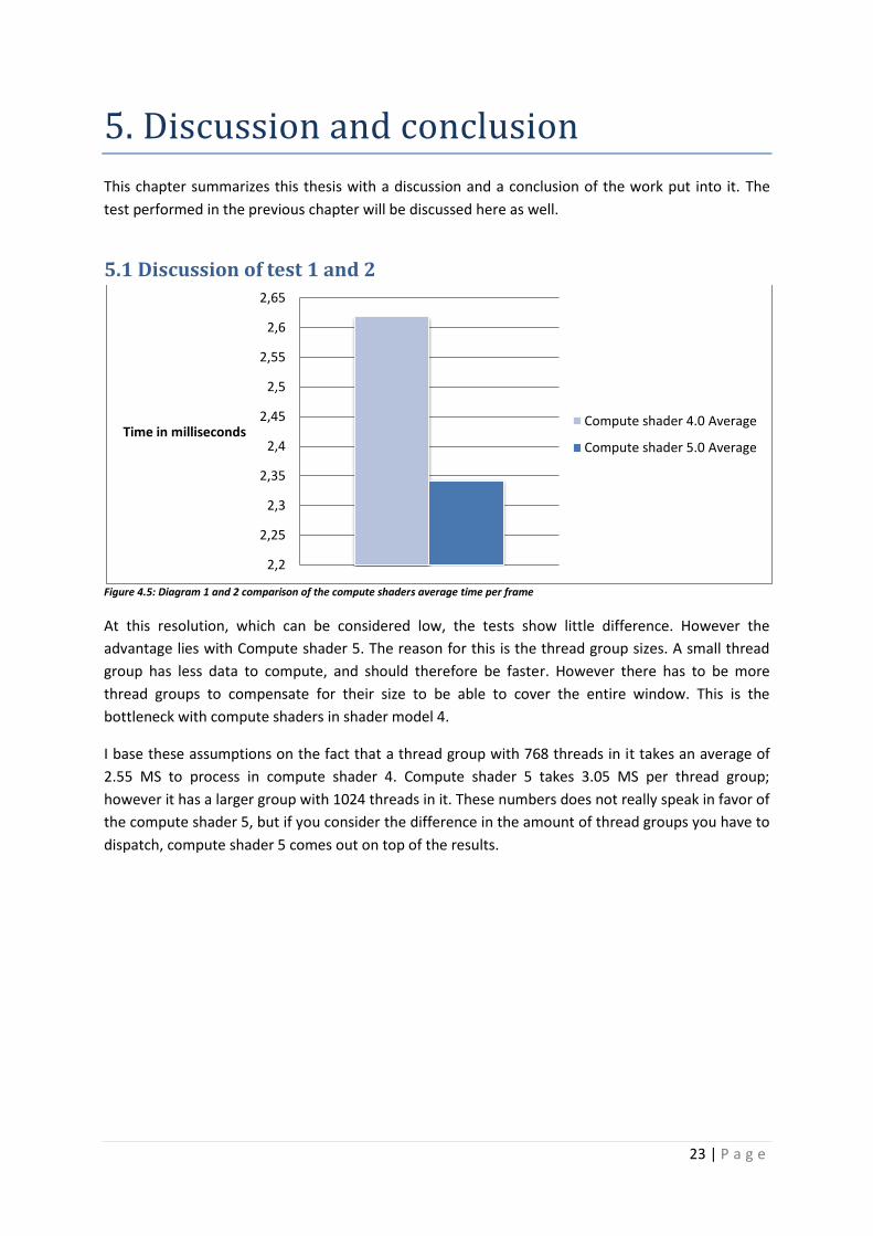
5.1 Discussion of test 1 and 2
Figure 4.5: Diagram 1 and 2 comparison of the compute shaders average time per frame
At this resolution, which can be considered low, the tests show little difference. However the
advantage lies with Compute shader 5. The reason for this is the thread group sizes. A small thread
group has less data to compute, and should therefore be faster. However there has to be more
thread groups to compensate for their size to be able to cover the entire window. This is the
bottleneck with compute shaders in shader model 4.
I base these assumptions on the fact that a thread group with 768 threads in it takes an average of
2.55 MS to process in compute shader 4. Compute shader 5 takes 3.05 MS per thread group;
however it has a larger group with 1024 threads in it. These numbers does not really speak in favor of
the compute shader 5, but if you consider the difference in the amount of thread groups you have to
dispatch, compute shader 5 comes out on top of the results.
2,2
2,25
2,3
2,35
2,4
2,45
2,5
2,55
2,6
2,65
Time in millisecondsCompute shader 4.0 Average
Compute shader 5.0 Average
24 | P a g e
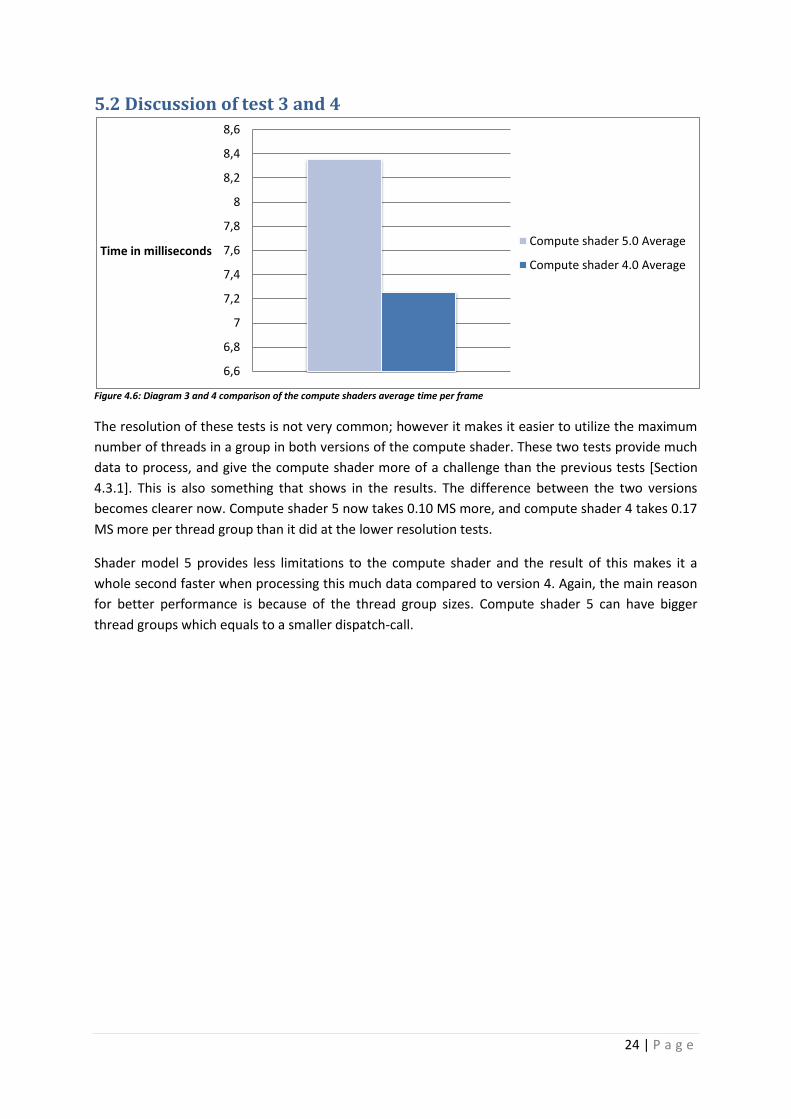
5.2 Discussion of test 3 and 4
Figure 4.6: Diagram 3 and 4 comparison of the compute shaders average time per frame
The resolution of these tests is not very common; however it makes it easier to utilize the maximum
number of threads in a group in both versions of the compute shader. These two tests provide much
data to process, and give the compute shader more of a challenge than the previous tests [Section
4.3.1]. This is also something that shows in the results. The difference between the two versions
becomes clearer now. Compute shader 5 now takes 0.10 MS more, and compute shader 4 takes 0.17
MS more per thread group than it did at the lower resolution tests.
Shader model 5 provides less limitations to the compute shader and the result of this makes it a
whole second faster when processing this much data compared to version 4. Again, the main reason
for better performance is because of the thread group sizes. Compute shader 5 can have bigger
thread groups which equals to a smaller dispatch-call.
6,6
6,8
7
7,2
7,4
7,6
7,8
8
8,2
8,4
8,6
Time in millisecondsCompute shader 5.0 Average
Compute shader 4.0 Average

25 | P a g e
5.3 Discussion This thesis focuses on deferred rendering using compute shaders, comparing performance between
compute shader 4 and 5. The hypothesis claims that deferred rendering performance between
Compute shaders in DirectX 10 and DirectX 11 is measurably better in DirectX 11. The results in
chapter 4 have proven this to be correct, where the differences were considerably better in shader
model 5.
The tests performed were basic, mainly testing the read and write capabilities of compute shaders.
These are still relevant though, since deferred rendering is much about just that. When using many
render reading from these takes time. Writing to a new resource takes time as well. Tests show a
difference of 16 FPS between the two models when rendering at a resolution of 2048x1152. That is
much considering it is the same code used for both tests. To give you a better perspective over these
numbers, that is approximately 2,36 million pixels that have to be written to a new buffer. Since the
prototype uses two render targets, twice of this amount has to be read from. All this is done in just
about 7 milliseconds. The potential of the compute shader is undeniable.
There is no documentation of how threads are processed on the GPU. That is why the reasoning
behind why compute shader 5 is faster than compute shader 4 is mainly based on the acquired test
results but also on the knowledge I have. Because of this, the reasoning may not be accurate.
However I think this is enough to give the reader and myself a reason behind the advantage of
compute shader 5.
The goal set up when starting this thesis has been reached. This has been achieved by investigating
the differences between deferred rendering implemented using compute shaders in DirecX 10 and
DirectX 11. Further investigations can be made on how the compute shader can improve deferred
rendering.
Further investigations could include having several instances of compute shaders to execute the
different phases of deferred rendering, such as lighting in addition to assembling the G-buffers. As
mentioned in Chapter 3, there are some issues to deferred rendering. There are solutions to these
problems that were too expensive to use before, however might be suitable to use with the compute
shader.

26 | P a g e
5.2 Conclusion The test application was developed prior to writing this report; however the hypothesis has been the
same since the beginning of this thesis. The tests performed in chapter 4 proved the hypothesis to be
correct in all cases, which was also something that I expected. The compute shader is limited to
DirectX 10 and 11; however this is not a problem any longer since the majority of users are up to
date with hardware. The responsibility is on the developer to implement these new features into
their games.
The application was made with the tests in mind to make it as easy as possible to perform the
different test cases. There are two variables you have to change to set the resolution and to set the
correct shader model to be used. Although the application applied the most basic implementation of
deferred rendering, it was enough to provide evidence of increased performance in shader model 5.
27 | P a g e
6. References
6.1 Bibliography 2 Thibieroz, N., Deferred Shading with Multisampling Anti-Aliasing in DirectX 10, in ShaderX7:
Advanced rendering techniques, W. Engel, Editor. 2009, Course technology, a part of Cengage Learning. P. 225-242.
5 Luna, F. D. (2008). Introduction to 3D game programming with DirectX 10. Plano, Texas: Wordware Publishing, Inc.
15 Thibieroz, N. (2004). ShaderX2: Shader Programming Tips & Tricks with DirectX 9. Plano, Texas: Wordware publishing, Inc. P. 251-269. Retrieved from: http://tog.acm.org/resources/shaderx/.
6.2 Papers 13 Luft, T. and others. Image Enhancement by Unsharp Masking the Depth Buffer in Proceedings of
ACM SIGGRAPH 2006.
14 Lance, W. Casting curved shadows on curved surfaces in Proceedings of ACM SIGGRAPH 1978.
6.3 Presentations 1 Boyd, C. Direct3D 11 Compute Shader, More Generality for Advanced Techniques. 2008.
Presented at Gamefest 2008.
6.4 Websites Link worked
3 Eisler, C. DirectX Then and Now (Part 1). http://craig.theeislers.com/2006/02/directx_then_and_now_part_1.php
210510
4 http://www.shacknews.com/onearticle.x/61231 210510
6 Hoxley, J. An Overview of Microsoft’s Direct3D 10 API. http://www.gamedev.net/reference/programming/features/d3d10overview/
210510
7 http://msdn.microsoft.com/en-us/library/bb205127%28v=VS.85%29.aspx 210510
8 http://msdn.microsoft.com/en-us/library/ff476906%28v=VS.85%29.aspx 210510
9 http://msdn.microsoft.com/en-us/library/ff476335%28v=VS.85%29.aspx#Unordered_Access
210510
10 http://store.steampowered.com/hwsurvey/ 210510
11 http://en.wikipedia.org/wiki/List_of_games_with_DirectX_10_support 210510
12 http://en.wikipedia.org/wiki/List_of_games_with_DirectX_11_support 210510
16 http://msdn.microsoft.com/en-us/library/bb172499%28v=VS.85%29.aspx 210510
17 http://msdn.microsoft.com/en-us/library/bb205120%28VS.85%29.aspx 210510
18 Calver, D. Photo-realistic Deferred Lighting. http://www.beyond3d.com/content/articles/19/1
210510
19 http://en.wikipedia.org/wiki/Blinn%E2%80%93Phong_shading_model 210510
20 http://msdn.microsoft.com/en-us/library/ff476578%28v=VS.85%29.aspx 210510
21 http://msdn.microsoft.com/en-us/library/ff476331%28v=VS.85%29.aspx 210510
22 http://msdn.microsoft.com/en-us/library/ff471442%28v=VS.85%29.aspx 210510
28 | P a g e
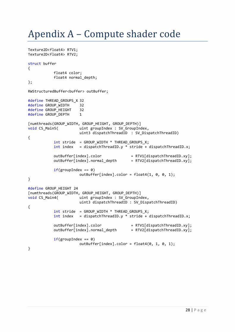
Apendix A – Compute shader code
Texture2D<float4> RTV1; Texture2D<float4> RTV2; struct buffer {
float4 color; float4 normal_depth; }; RWStructuredBuffer<buffer> outBuffer; #define THREAD_GROUPS_X 32 #define GROUP_WIDTH 32 #define GROUP_HEIGHT 32 #define GROUP_DEPTH 1 [numthreads(GROUP_WIDTH, GROUP_HEIGHT, GROUP_DEPTH)] void CS_Main5( uint groupIndex : SV_GroupIndex,
uint3 dispatchThreadID : SV_DispatchThreadID) { int stride = GROUP_WIDTH * THREAD_GROUPS_X; int index = dispatchThreadID.y * stride + dispatchThreadID.x; outBuffer[index].color = RTV1[dispatchThreadID.xy]; outBuffer[index].normal_depth = RTV2[dispatchThreadID.xy]; if(groupIndex == 0) outBuffer[index].color = float4(1, 0, 0, 1); } #define GROUP_HEIGHT 24 [numthreads(GROUP_WIDTH, GROUP_HEIGHT, GROUP_DEPTH)] void CS_Main4( uint groupIndex : SV_GroupIndex,
uint3 dispatchThreadID : SV_DispatchThreadID) { int stride = GROUP_WIDTH * THREAD_GROUPS_X; int index = dispatchThreadID.y * stride + dispatchThreadID.x; outBuffer[index].color = RTV1[dispatchThreadID.xy]; outBuffer[index].normal_depth = RTV2[dispatchThreadID.xy]; if(groupIndex == 0) outBuffer[index].color = float4(0, 1, 0, 1); }
29 | P a g e
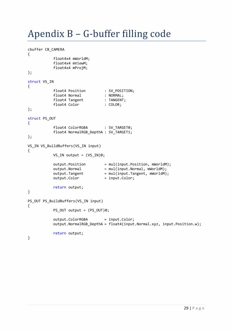
Apendix B – G-buffer filling code
cbuffer CB_CAMERA { float4x4 mWorldM; float4x4 mViewM; float4x4 mProjM; }; struct VS_IN { float4 Position : SV_POSITION; float4 Normal : NORMAL; float4 Tangent : TANGENT; float4 Color : COLOR; }; struct PS_OUT { float4 ColorRGBA : SV_TARGET0; float4 NormalRGB_DepthA : SV_TARGET1; }; VS_IN VS_BuildBuffers(VS_IN input) { VS_IN output = (VS_IN)0; output.Position = mul(input.Position, mWorldM); output.Normal = mul(input.Normal, mWorldM); output.Tangent = mul(input.Tangent, mWorldM); output.Color = input.Color; return output; } PS_OUT PS_BuildBuffers(VS_IN input) { PS_OUT output = (PS_OUT)0; output.ColorRGBA = input.Color; output.NormalRGB_DepthA = float4(input.Normal.xyz, input.Position.w); return output; }