The California Central Valley Groundwater-Surface Water

Simulation Model

C2VSim Overview

Charles Brush Modeling Support Branch, Bay-Delta Office

California Department of Water Resources, Sacramento, CA

CWEMF C2VSim Workshop January 23, 2013

2

Outline

Background and Development History

C2VSim Framework

Coarse-Grid and Fine-Grid Versions

Future Directions

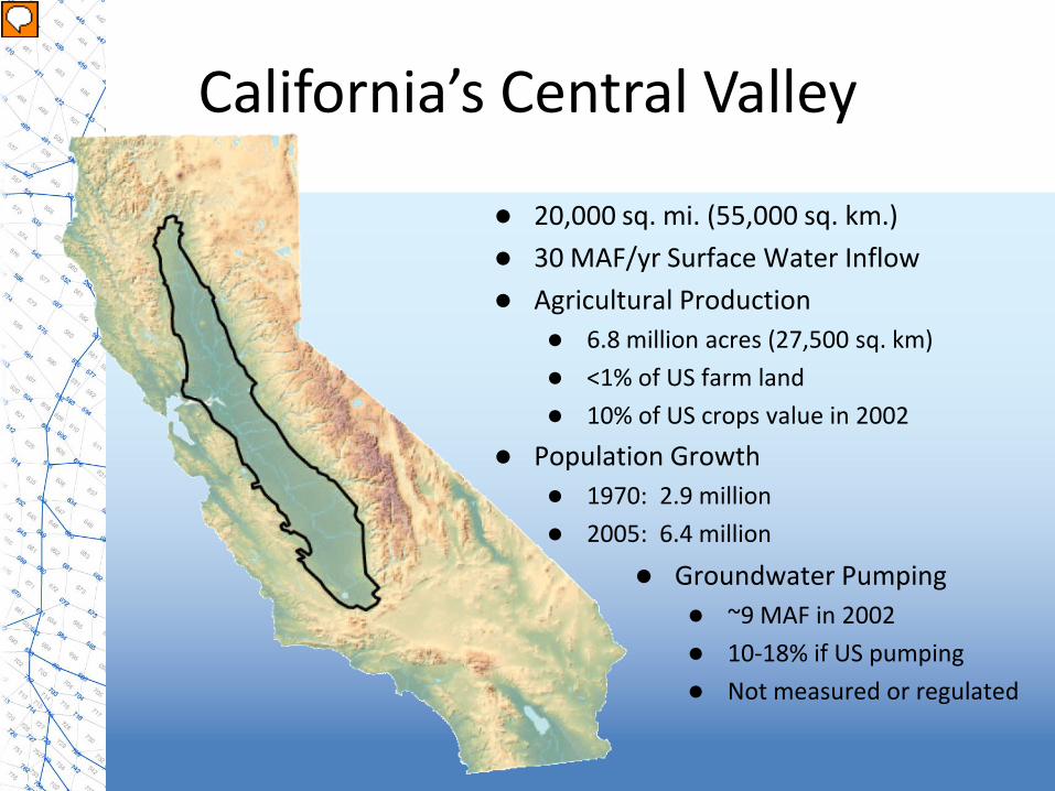
California’s Central Valley

20,000 sq. mi. (55,000 sq. km.) 30 MAF/yr Surface Water Inflow Agricultural Production

6.8 million acres (27,500 sq. km) <1% of US farm land 10% of US crops value in 2002

Population Growth 1970: 2.9 million 2005: 6.4 million

Groundwater Pumping ~9 MAF in 2002 10-18% if US pumping Not measured or regulated

4

C2VSim Development

Derived from the CVGSM model – WY 1922-1980 Boyle & JM Montgomery (1990) – WY 1981-1998 CH2M Hill for CVPIA PEIS

Steady modification – DWR IWFM/C2VSim development began in 2000 – IWFM process and solver improvements – C2VSim data sets reviewed and refined – C2VSim input data extended through WY 2009

Calibration – PEST parameter estimation program – Three phases: Regional, Local, Nodal – Calibration Period: WY 1973-2003 in phases 1 & 2, 1922-2004

in phase 3

Release – C2VSim 3.02-CG released December 2012 – C2VSim 3.02-FG expected summer 2013

5

C2VSim Applications

- CalSim 3 groundwater component

- Integrated Regional Water Management Plans

- Stream-groundwater flows

- Climate change assessments

- Groundwater storage investigations

- Planning studies

- Ecosystem enhancement scenarios

- Infrastructure improvements

- Impacts of operations on Delta flows

6

C2VSim Versions

C2VSim CG 3.02 (R367): Release Version – Current version, released December 2012 – Water Years 1922-2009, monthly time step – IWFM version 3.02

C2VSim FG 3.02 (R356): Draft Version – Based on C2VSim 3.02 CG of Jan 2012 – Refine rivers, inflows, land use – Upgrade to match CG version before release – Expected release in Summer 2013

Planned Improvements – C2VSim 3.02 CG/FG: Extend to WY 2011 or 2012 – C2VSim 4.0 FG: Element-level land use, crop and

diversion data

7

C2VSim Coarse Grid

DWR Web Site – Model files – Documetation – C2VSim ArcGIS GUI – IWFM Application – IWFM Tools

Support

– Training: IWFM and C2VSim workshops will be offered through CWEMF

– Technical support: Email and telephone

A Google search for “C2VSim” brings up this page

“C2VSim CG-3.02”

8

C2VSim Portal

Interactive Web Site – Tutorial Files – Project Files – Collaboration – Message Board – User/Password for

additional access

https://msb.water.ca.gov/c2vsim/-/document_library/view/140143

C2VSim Coarse-Grid

Finite Element Grid – 3 Layers or 9 Layers – 1393 Nodes & 1392 Elements

Surface Water System – 75 River Reaches, 2 Lakes – 243 Surface Water Diversions – 38 Inflows, 11 Bypasses – 210 Small-Stream Watersheds

Land Use Process – 21 Subregions (DSAs) – 4 Land Use Types

Simulation periods – 10/1921-9/2009 (88 yrs) – runs in 3-6 min

IWFM version 3.02

“C2VSim CG-3.02”

10

C2VSim Framework

• Nodal coordinates • Nodes form elements • Vertical aquifer stratigraphy • Lakes • River nodes • River reaches & flow network • Element properties • Pumping wells • Assign elements to subregions

Pre-processor

Nodes X-Y Grid

– UTM 10N – X = Easting – Y = Northing

Convert to FT

– FACT = 3.2808

Elements

Finite Element Mesh – 4 nodes = quadrilateral – 3 nodes = triangle

1392 elements

‘Hangs’ from Ground Surface

Stratigraphy

250 ft

60 ft

-20 ft

-280 ft

Stratigraphy

At each node: Land Surface Elevation For each layer

– Aquiclude thickness – Aquifer thickness

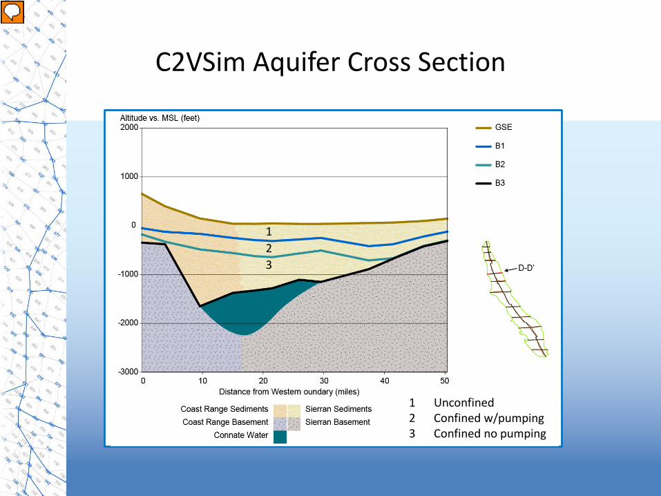
C2VSim Aquifer Cross Section

1 2 3

1 Unconfined 2 Confined w/pumping 3 Confined no pumping

C2VSim Aquifer Thicknesses

Presenter

Presentation Notes

Steven Springhorn of DWR has developed a new map of the base of fresh water in the Sacramento Valley.

Three dimensional view (looking north) of the base of fresh water surface

Base of Fresh Water

River Nodes and Reaches

Listed by Reach Nodes linked to mesh

River Nodes and Reaches

Rating table for each node at the end of the file

River Nodes and Reaches

Rating table for each node at the end of the file

0

5

10

15

20

25

0 10,000 20,000 30,000

Dep

th (f

t)

Flow (cfs)

Lakes

Groups of Elements

Outflow = River Node #

Element Characteristics

• Precipitation data column

• River node receiving drainage

• Subregion

• Soil type A = 1 B = 2 C = 3 D = 4

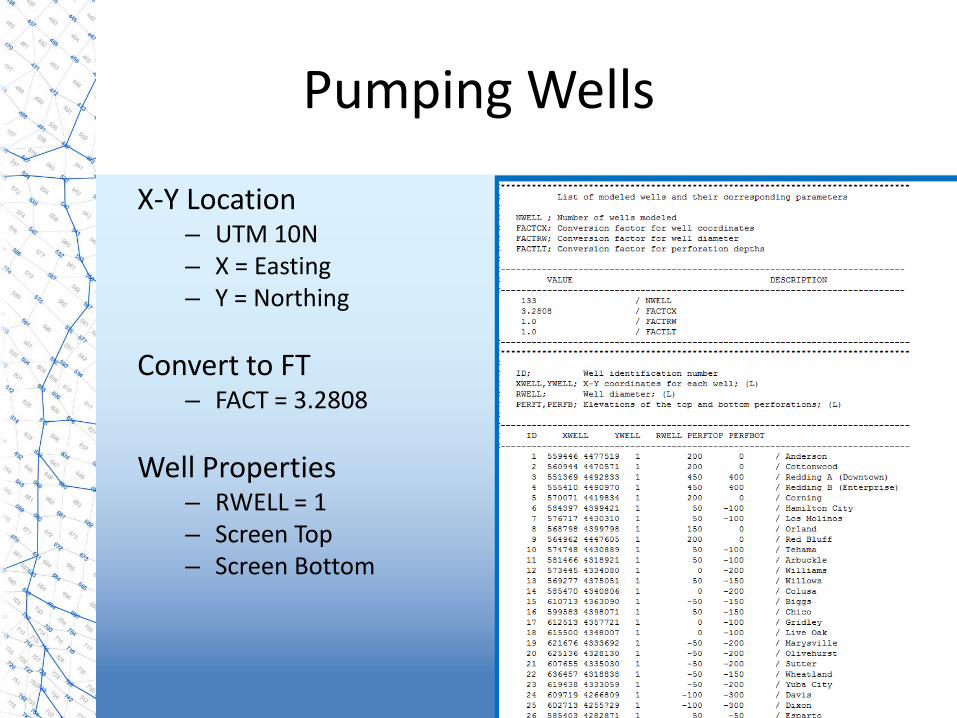
Pumping Wells

X-Y Location – UTM 10N – X = Easting – Y = Northing

Convert to FT

– FACT = 3.2808

Well Properties – RWELL = 1 – Screen Top – Screen Bottom

Calibrated Parameters

Aquifer nodes – Conductivity – Storage – Subsidence

River nodes

– Conductance

Unsaturated Zone – Porosity – Conductivity

Soil properties – Field capacity – Porosity – Recharge factor – Curve Numbers

Small Watersheds

– Field capacity – Porosity – Conductivity – Discharge threshold – Recession coefficients

26

Calibration with PEST

27

Calibration with PPEST

i

PPEST

PPEST

RMSE

C2VSim Calibration • Calibrate parameter values at each

model node and layer

• Using computers at the USDOE National Energy Research Scientific Computing Center (NERSC)

– Carver • IBM iDataPlex • 3,200 CPU cores, 34 Tflop/s

• Comparison:

PPs Compter Run Time

R300 137 15 PCs 1 week

R326 394 15 PCs 3 weeks

R346 1393 15 PCs 16 weeks

R346 1393 NERSC 2 weeks

Calibration Observations

Groundwater Heads – 56,947 observations at 1,145 wells

Vertical Head Difference

– 3,017 observations at 121 well pairs

Surface Water Flow – 5,636 observations at 21 locations

Stream-Groundwater Flows

– Average annual rates on 24 reaches

30

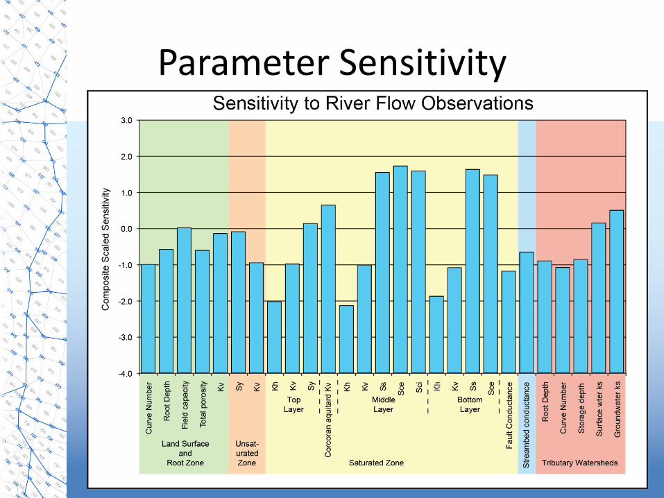
Parameter Sensitivity

Ungaged Watersheds

Land Surface

Streambed

Unsaturated Zone

Saturated Zone

Groundwater Head

River Flow

Groundwater Gradient

Stream- Groundwater

Flow

Parameters Observations

Parameter Sensitivity

Parameter Sensitivity

Parameter Sensitivity

Parameter Sensitivity

Hydraulic Conductivity Layer 1 Layer 2

Storage Parameters Layer 1 Layer 2

River-Bed Conductance

Model Performance

Units: Heads and subsidence in feet, flows in acre-feet Head and flow observations from October 1975 to September 2003, Subsidence observations from September 1957 to May 2004

Observation Type No.

Observation Sites

No. Observations Range

Groundwater heads 1,378 62,981 1,252 Vert. Groundwater Head Difference 163 3,017 698 River Flows 22 5,636 6,561,453 River-Groundwater Flows 33 33 38,117 Subsidence 24 3,700 6.2 TOTAL 1,620 75,367

Observation Type Root Mean Squared

Error Residual RMSE

Range Residual Range

Groundwater heads 65.4 2.14 0.052 0.002 Vert. Groundwater Head Difference 96.2 -13.3 0.138 -0.019 River Flows 145,591 -13,720 0.022 -0.002 River-Groundwater Flows 8,875 3,620 0.233 0.095 Subsidence 17.4 -11.5 2.81 -1.86

Groundwater Heads 62,981 observations at 1,378 wells

RMSE/Range = 0.052 Ft

Residual/Range = 0.002 Ft

Surface Water Flows 5,636 observations at 22 gages

RMSE/Range = 0.022 Ac-Ft/mo Residual/Range = -0.002 Ac-Ft/mo

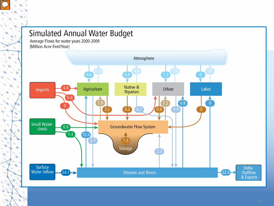
41

42

Urban Water Supply

River-Groundwater Flows Groundwater Pumping

Change in Groundwater Storage

Sacramento River reach near Chico

43

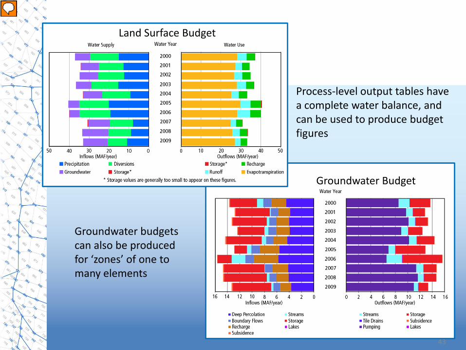
Land Surface Budget

Groundwater Budget

Process-level output tables have a complete water balance, and can be used to produce budget figures

Groundwater budgets can also be produced for ‘zones’ of one to many elements

44

Water Table Altitude Produced from IWFM’s TecPlot® output files

45

IWFM

46

IWFM Water Balance Diagram

47

• Land Surface Processes - Land and Water Use Budget - Root Zone Budget

• Groundwater Process

- Groundwater Budget - Z-Budget Budget

• Surface Water Processes

- Stream Reach Budget - Lake Budget

• Small-Streams Watershed Process

- Small Watershed Budget

C2VSim Model

END