Embed Size (px)
Citation preview

Agenda
● What are anomalies ?
● Types of anomaly detection
● Normal distribution
● Multivariate normal distribution
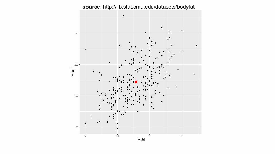
● Case study - body fat dataset
● Conclusions
● References

What are anomalies ?Concepts and Definitions
● Small number of observations that do not conform the behavior from the the rest of the database
● Also known as outliers
● Generally less than 5% of total population

source: http://lib.stat.cmu.edu/datasets/bodyfat
source: http://lib.stat.cmu.edu/datasets/bodyfat

source: http://lib.stat.cmu.edu/datasets/bodyfat
Concepts and Definitions
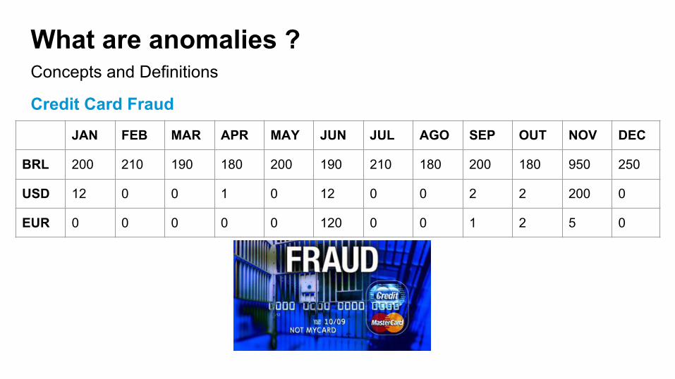
What are anomalies ?
Credit Card Fraud
JAN FEB MAR APR MAY JUN JUL AGO SEP OUT NOV DEC
BRL 200 210 190 180 200 190 210 180 200 180 950 250
USD 12 0 0 1 0 12 0 0 2 2 200 0
EUR 0 0 0 0 0 120 0 0 1 2 5 0

Concepts and Definitions
What are anomalies ?
Credit Card Fraud
JAN FEB MAR APR MAY JUN JUL AGO SEP OUT NOV DEC
BRL 200 210 190 180 200 190 210 180 200 180 950 250
USD 12 0 0 1 0 12 0 0 2 2 200 0
EUR 0 0 0 0 0 120 0 0 1 2 5 0

Concepts and Definitions
What are anomalies ?
Factory Inspection
ID Temperature (Celsius) Rotation(RPM)
100 10.89 10
110 9.78 10
120 45.23 15
130 9.91 10
140 9.23 11

Concepts and Definitions
What are anomalies ?
Factory Inspection
ID Temperature (Celsius) Rotation(RPM)
100 10.89 10
110 9.78 10
120 45.23 15
130 9.91 10
140 9.23 11

Concepts and Definitions
What are anomalies ?
Cyber Security
timestamp IP command
2015-01-10 15:05:05 10.10.1.10 open port 80
2015-01-10 15:25:10 10.10.1.10 request content
2015-01-10 15:27:25 10.10.1.10 open port 22
2015-01-10 16:15:36 10.10.1.10 send command as root

Concepts and Definitions
Types of Anomaly Detection
● By learning method○ Supervised○ Unsupervised○ Semi-supervised
● By dimensionality○ Univariate (one dimension)○ Multivariate (multiple dimensions)
● By characteristic○ Point○ Contextual

Concepts and Definitions - By learning method
Types of Anomaly Detection
● Supervised Learning
Column A Column B Column C Anomalous (label)
... ... ... FALSE
... ... ... FALSE
... ... ... TRUE

Concepts and Definitions - By learning method
Types of Anomaly Detection
● Unsupervised Learning
Column A Column B Column C
... ... ...
... ... ...
... ... ...
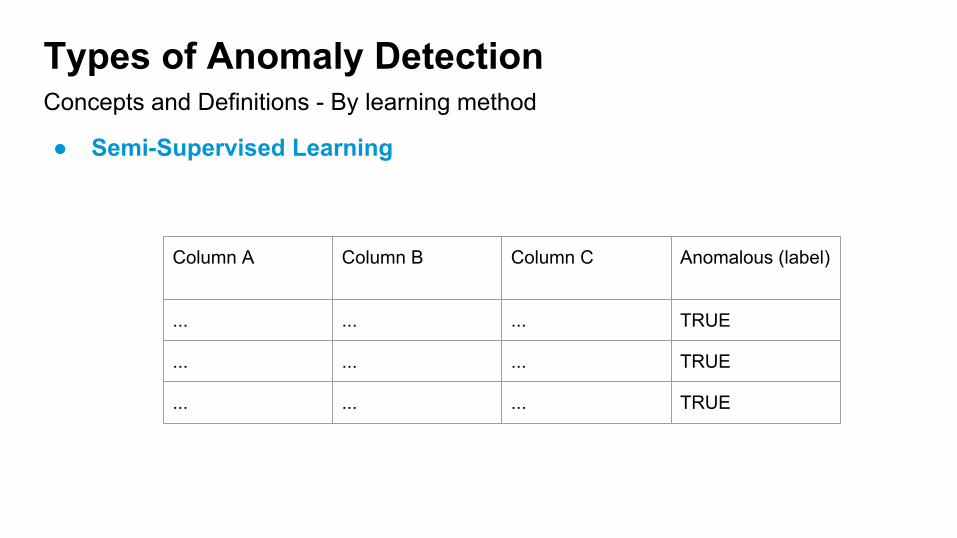
Concepts and Definitions - By learning method
Types of Anomaly Detection
● Semi-Supervised Learning
Column A Column B Column C Anomalous (label)
... ... ... TRUE
... ... ... TRUE
... ... ... TRUE

Concepts and Definitions - By dimensionality
Types of Anomaly Detection
● Univariate
Temperature
121
118
121
104
120
...
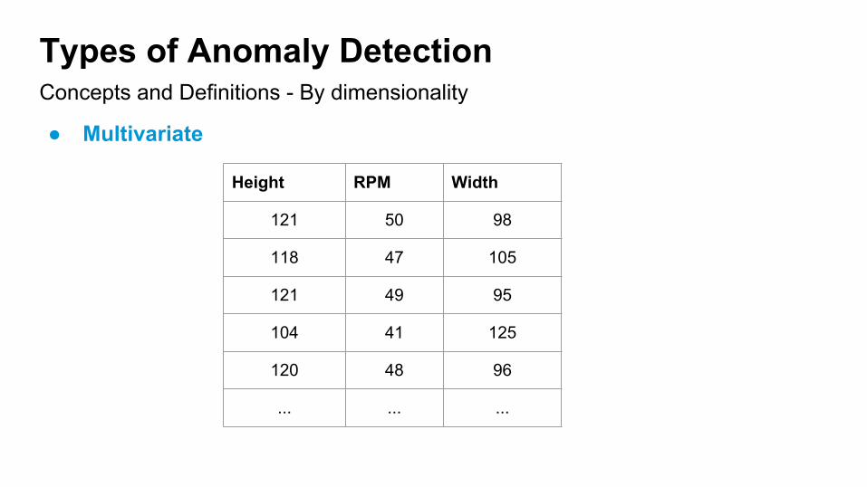
Concepts and Definitions - By dimensionality
Types of Anomaly Detection
● Multivariate
Height RPM Width
121 50 98
118 47 105
121 49 95
104 41 125
120 48 96
... ... ...

Concepts and Definitions - By characteristic
Types of Anomaly Detection
● Point
Temperature
121
118
121
104
120
...

Concepts and Definitions - By characteristic
Types of Anomaly Detection
● Contextual
Timestamp CPU (%)
2015-12-20 08:30:00 5
2015-12-20 10:30:00 12
2015-12-20 12:30:00 5
2015-12-20 14:30:00 7
2015-12-20 16:30:00 11
…. ...
image source: https://github.com/twitter/AnomalyDetection/raw/master/figs/Fig1.png

Anomaly detection techniques
Algorithms
● Normal Distribution
● Multivariate Normal Distribution

Algorithms
Normal Distribution
● Point, univariate and supervised
Temperature Anomaly
121 F
118 F
119 F
120 F
104 T
121 F
119 F
122 F
120 F
120 F

Requirement
Normal Distribution
● Does the data distribution follows a bell shape curve pattern ?
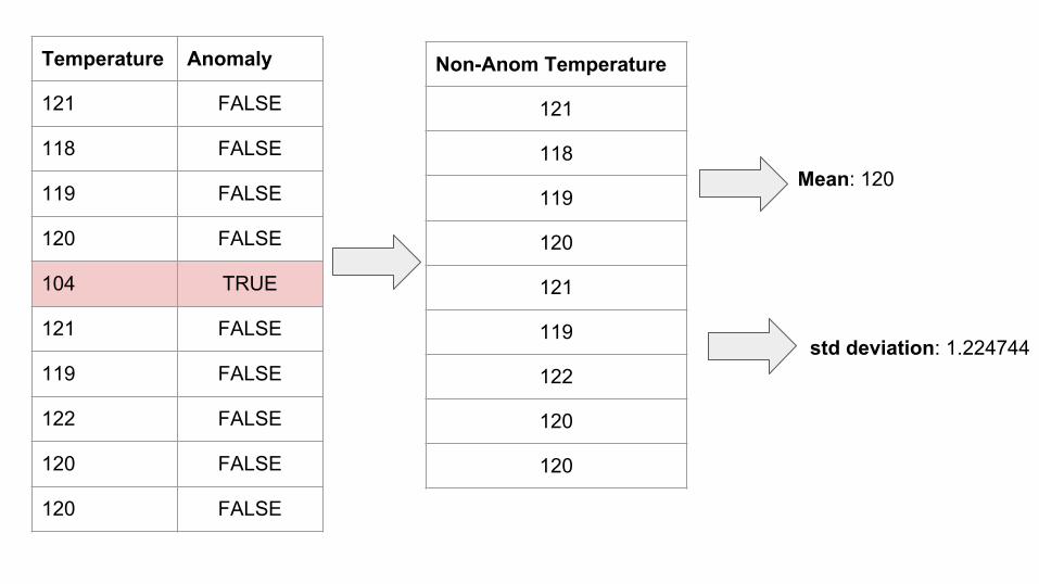
Temperature Anomaly
121 FALSE
118 FALSE
119 FALSE
120 FALSE
104 TRUE
121 FALSE
119 FALSE
122 FALSE
120 FALSE
120 FALSE
Non-Anom Temperature
121
118
119
120
121
119
122
120
120
Mean: 120
std deviation: 1.224744

Algorithms
Normal Distribution
● Probability density function
= 120
= 1.224744

Algorithms
Normal Distribution
● Probability density function

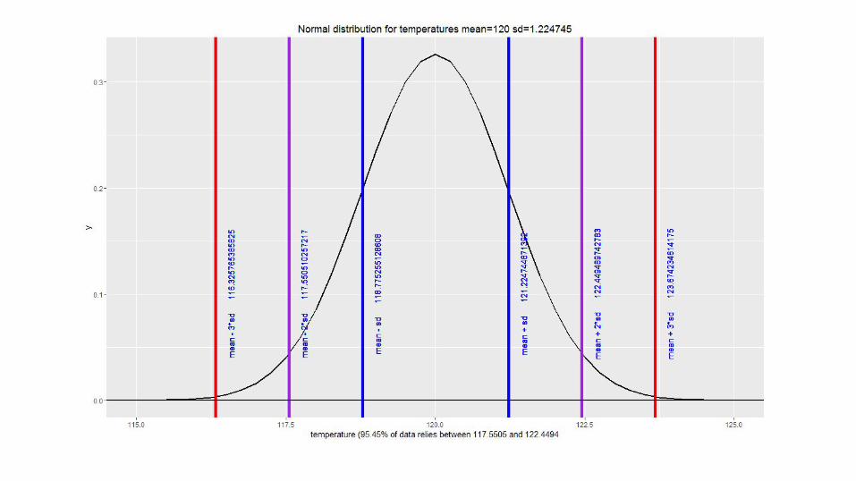
Algorithms
Normal Distribution
● Probability density functionData distribution
● 68.27% = values 1 sd away from the mean
● 95.45% = values 2 sd away from the mean
● 99.73% = values 3 sd away from the mean
Therefore
● 31.73% = values beyond 1 sd from the mean
● 4.55% = values beyond 2 sd from the mean
● 0.27% = values beyond 3 sd from the mean

Algorithms
Normal Distribution
● Probability density function
Temp. Mean SD Density
121 120 1.224745 0.2333993
118 120 1.224745 0.08586282
119 120 1.224745 0.2333993
120 120 1.224745 0.325735
104 120 1.224745 2.838368e-38
121 120 1.224745 0.2333993
119 120 1.224745 0.2333993
122 120 1.224745 0.08586282
120 120 1.224745 0.325735
120 120 1.224745 0.325735

Algorithms
Normal Distribution
● Final step is threshold determination
● Supervised approach - use labeled data to find best threshold

Temp. Mean SD Prob. Dens < 0.3 Dens < 0.2 Dens < 0.1 Dens < 0.05
121 120 1.224745 0.2333993 T F F F
118 120 1.224745 0.08586282 T T T F
119 120 1.224745 0.2333993 T F F F
120 120 1.224745 0.325735 F F F F
104 120 1.224745 2.838368e-38 T T T T
121 120 1.224745 0.2333993 T F F F
119 120 1.224745 0.2333993 T F F F
122 120 1.224745 0.08586282 T T T F
120 120 1.224745 0.325735 F F F F
120 120 1.224745 0.325735 F F F F

Temp. Mean SD Prob. Dens < 0.3 Dens < 0.2 Dens < 0.1 Dens < 0.05
121 120 1.224745 0.2333993 T F F F
118 120 1.224745 0.08586282 T T T F
119 120 1.224745 0.2333993 T F F F
120 120 1.224745 0.325735 F F F F
104 120 1.224745 2.838368e-38 T T T T
121 120 1.224745 0.2333993 T F F F
119 120 1.224745 0.2333993 T F F F
122 120 1.224745 0.08586282 T T T T
120 120 1.224745 0.325735 F F F F
120 120 1.224745 0.325735 F F F F

Algorithms
Multivariate Normal Distribution
● Point, multivariate and supervised
Temp. Weight Anomaly
121 67 F
118 66 F
119 74 F
120 75 F
104 45 T
121 86 F
119 56 F
122 55 F
120 99 T
120 65 F

Temp. * Temp. mean Temp. sd Weight * Weight mean Weight sd
121 120 1.309307 67 68 10.25392
118 120 1.309307 66 68 10.25392
119 120 1.309307 74 68 10.25392
120 120 1.309307 75 68 10.25392
121 120 1.309307 86 68 10.25392
119 120 1.309307 56 68 10.25392
122 120 1.309307 55 68 10.25392
120 120 1.309307 65 68 10.25392
Multivariate Normal Distribution
* = Non-Anomalous observations only

Temp. Temp. Dens. Weight Weight Dens. Final Dens. (temp dens. x weight dens.) Anomaly
121 0.2276141 67 0.0387217449 0.2276141*0.0387217449 = 0.008813 F
118 0.09488369 66 0.0381732505 0.0948836 * 0.0381732505 = 0.0036220 F
119 0.2276141 74 0.0327846726 0.2276141 * 0.0327846726 = 0.0074622 F
120 0.3046972 75 0.0308192796 0.3046971 * 0.0308192796 = 0.0093905 F
104 1.139061e-33 45 0.0031441128 1.139061e-33 * 0.0031441128= 3.58133e-36 T
121 0.2276141 86 0.0083344364 0.2276141 * 0.0083344 = 0.0018970 F
119 0.2276141 56 0.0196165609 0.2276141 * 0.0196165 = 0.0044650 F
122 0.09488369 55 0.0174177236 0.0948836 * 0.0174177 = 0.0016526 F
120 0.3046972 99 0.0004030011 0.3046971 * 0.0004030 = 0.0001227 T
120 0.3046972 65 0.0372763042 0.3046971 * 0.0372763 = 0.0113579 F

Temp. Weight Final Dens. < 0.005 < 0.002 < 0.001 Anomaly
121 50 0.008813 F F F F
118 50 0.0036220 T F F F
119 51 0.0074622 F F F F
120 50 0.0093905 F F F F
104 53 3.58133e-36 T T T T
121 50 0.0018970 T T F F
119 51 0.0044650 T F F F
122 51 0.0016526 T T F F
120 45 0.0001227 T T T T
120 50 0.0113579 F F F F
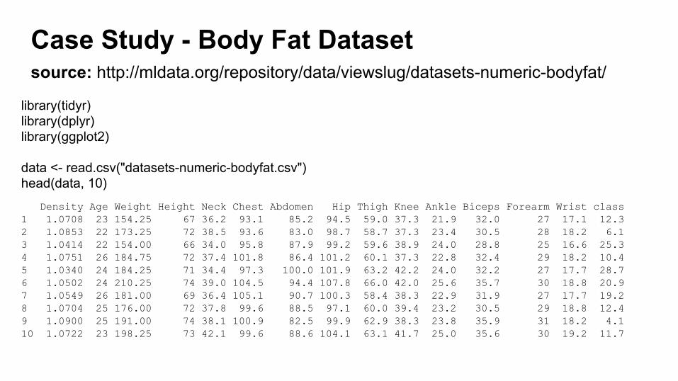
source: http://mldata.org/repository/data/viewslug/datasets-numeric-bodyfat/
Case Study - Body Fat Dataset
library(tidyr)library(dplyr)library(ggplot2)
data <- read.csv("datasets-numeric-bodyfat.csv")head(data, 10)
Density Age Weight Height Neck Chest Abdomen Hip Thigh Knee Ankle Biceps Forearm Wrist class1 1.0708 23 154.25 67 36.2 93.1 85.2 94.5 59.0 37.3 21.9 32.0 27 17.1 12.32 1.0853 22 173.25 72 38.5 93.6 83.0 98.7 58.7 37.3 23.4 30.5 28 18.2 6.13 1.0414 22 154.00 66 34.0 95.8 87.9 99.2 59.6 38.9 24.0 28.8 25 16.6 25.34 1.0751 26 184.75 72 37.4 101.8 86.4 101.2 60.1 37.3 22.8 32.4 29 18.2 10.45 1.0340 24 184.25 71 34.4 97.3 100.0 101.9 63.2 42.2 24.0 32.2 27 17.7 28.76 1.0502 24 210.25 74 39.0 104.5 94.4 107.8 66.0 42.0 25.6 35.7 30 18.8 20.97 1.0549 26 181.00 69 36.4 105.1 90.7 100.3 58.4 38.3 22.9 31.9 27 17.7 19.28 1.0704 25 176.00 72 37.8 99.6 88.5 97.1 60.0 39.4 23.2 30.5 29 18.8 12.49 1.0900 25 191.00 74 38.1 100.9 82.5 99.9 62.9 38.3 23.8 35.9 31 18.2 4.110 1.0722 23 198.25 73 42.1 99.6 88.6 104.1 63.1 41.7 25.0 35.6 30 19.2 11.7
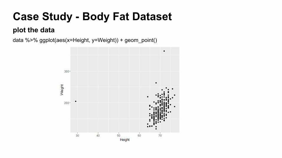
Case Study - Body Fat Dataset
data %>% ggplot(aes(x=Height, y=Weight)) + geom_point()
plot the data

Case Study - Body Fat Datasetplot histogram from each feature
hist(data$Height, breaks=35) hist(data$Weight, breaks = 30)
Is the distribution similar to a bell shape curve ?

Case Study - Body Fat Dataset
df_prob <- data %>% select(Height, Weight) %>% mutate(Height.Prob = dnorm(Height, mean(Height), sd(Height)) ) %>% mutate(Weight.Prob = dnorm(Weight, mean(Weight), sd(Weight)) ) %>% mutate(Dens.Prob = Height.Prob * Weight.Prob)
Height Weight Height.Prob Weight.Prob Dens.Prob1 67 154.25 8.181724e-02 9.542426e-03 7.807349e-042 72 173.25 8.996915e-02 1.332379e-02 1.198730e-033 66 154.00 6.436414e-02 9.474175e-03 6.097971e-044 72 184.75 8.996915e-02 1.331039e-02 1.197524e-035 71 184.25 1.022848e-01 1.335342e-02 1.365852e-036 74 210.25 5.580939e-02 7.691614e-03 4.292643e-047 69 181.00 1.059974e-01 1.354066e-02 1.435275e-038 72 176.00 8.996915e-02 1.350743e-02 1.215252e-039 74 191.00 5.580939e-02 1.247563e-02 6.962574e-0410 73 198.25 7.351777e-02 1.093521e-02 8.039323e-0411 74 186.25 5.580939e-02 1.315925e-02 7.344099e-0412 76 216.00 2.578613e-02 6.125433e-03 1.579512e-04
calculate probability density
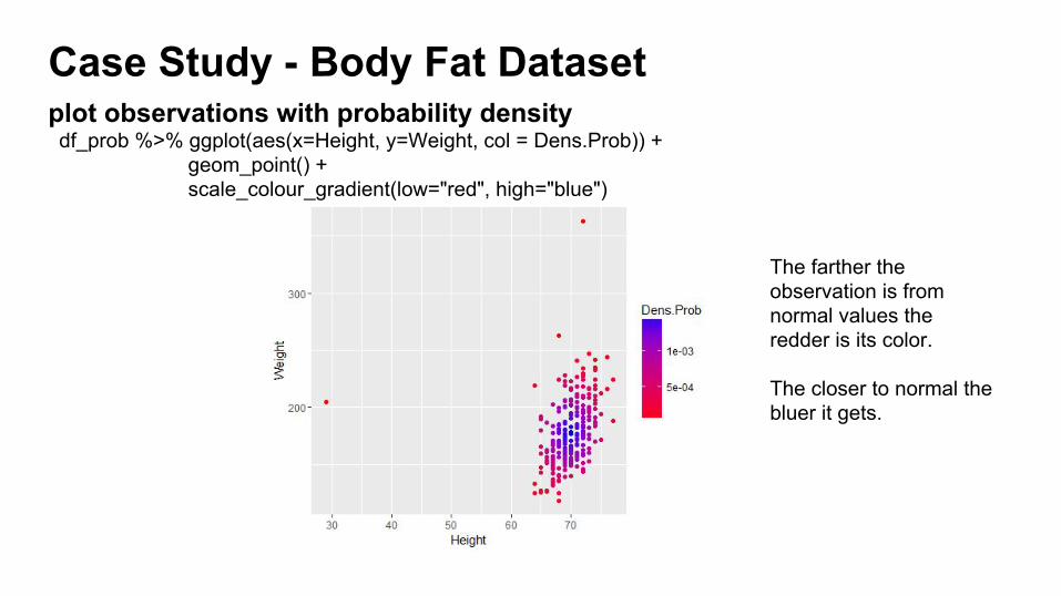
Case Study - Body Fat Datasetdf_prob %>% ggplot(aes(x=Height, y=Weight, col = Dens.Prob)) +
geom_point() + scale_colour_gradient(low="red", high="blue")
plot observations with probability density
The farther the observation is from normal values the redder is its color.
The closer to normal the bluer it gets.

Case Study - Body Fat Datasetdf_prob <- data %>% select(Height, Weight) %>% mutate(Height.Prob = dnorm(Height, mean(Height), sd(Height)) ) %>% mutate(Weight.Prob = dnorm(Weight, mean(Weight), sd(Weight)) ) %>% mutate(Dens.Prob = Height.Prob * Weight.Prob)
Height Weight Height.Prob Weight.Prob Dens.Prob1 29 205.00 2.942229e-28 9.157587e-03 2.694371e-302 72 363.15 8.996915e-02 3.982465e-11 3.582990e-123 68 262.75 9.661887e-02 2.323502e-04 2.244942e-054 76 244.25 2.578613e-02 1.147767e-03 2.959648e-055 77 224.50 1.569459e-02 4.078622e-03 6.401233e-056 73 247.25 7.351777e-02 9.100195e-04 6.690260e-057 74 241.75 5.580939e-02 1.381655e-03 7.710932e-058 64 125.00 3.193679e-02 2.521546e-03 8.053006e-059 65 125.75 4.703915e-02 2.641563e-03 1.242569e-0410 74 234.75 5.580939e-02 2.234647e-03 1.247143e-04
selecting most anomalous observations

Case Study - Body Fat Datasetdf_prob %>% mutate(Anom = Dens.Prob <= 1.247143e-04) %>% mutate(Height.Mean = mean(Height), Weight.Mean = mean(Weight)) %>% ggplot(aes(x=Height, y=Weight, col=Anom)) + geom_point() + geom_point(aes(x=Height.Mean, y = Weight.Mean), col = "black")
plot most anomalous observations with different color

Conclusions
● Anomalies are small group of data that behaves differently from what is considered normal
● There are many applications for anomaly detection● There are several types of anomalies● Normal distribution can be used to detect anomalies provided that the
features follow a bell shaped curve distribution● Multivariate normal distribution can be used when more than one feature
must be considered

References
1. Anomaly Detection: A Tutorial - Arindam Banerjee, Varun Chandola, Vipin Kumar, Jaideep Srivastava, Aleksandar Lazarevica. https://www.siam.org/meetings/sdm08/TS2.ppt
2. Anomaly Detection - a. http://www.holehouse.org/mlclass/15_Anomaly_Detection.html
3. Anomaly Detection - Machine Learning Class Notes - Lecture 16: Anomaly Detectiona. http://dnene.bitbucket.org/docs/mlclass-notes/lecture16.html
4. Normal Distributiona. https://en.wikipedia.org/wiki/Normal_distribution


![Classifier Two-Sample Test for Video Anomaly Detections · Video anomaly detections are usually studied under the supervised settings [2, 3, 5, 6, 14, 19, 21, 25]. The most common](https://img.pdfslide.us/doc/110x75/606deafa63b761261f1bed98/classiier-two-sample-test-for-video-anomaly-video-anomaly-detections-are-usually.jpg)