Breeding for wood quality april 2007

1

Breeding for Wood Quality;Acoustic Tools and

Technology

2007 AFG & IUFRO SPWG Joint ConferenceHobart, Tasmania – April 2007

Peter Carter – Chief Executive, Fibre-gen

2

Contents

• Why acoustics?• How acoustics work• Results, tricks and traps• Who’s doing it?• Conclusions

3

Why? Global developments• Resource wood quality is changing, target of value improvement

– Global emphasis on structural and appearance qualities– Age of clearfall declining, log quality more variable– Tree breeding has improved volume more than quality

• Increased attention to quality standards eg NZ Standard 3622– Development of ‘verified visual’ grading (sample proof tested)– Price differential in lumber and engineered wood markets– Mills sensitive to stiffness of smaller diameter young wood

• New tools – Structural and LVL mills can now measure stiffness

Breeding for stiffness will enhance business returns

4

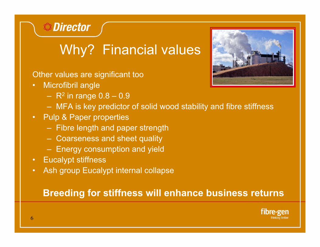
Why? Financial values

What is stiffness worth – a couple of examples• Verified visual grading – batch pass/fail

– VSG8 lumber premium is NZ$100/m3 ($450 vs $350)– At 55% conversion, 80% structural, equates to $36/m3 log– At 600m3/ha, 70% sawlog, 27 yrs, 8%, equates to $1,893/ha

• MSG lumber – incremental benefit– MGP8 lumber premium is NZ$250/m3

– 0.1km/sec gives 5% more MGP8, worth $12.50/m3

– At 600m3/ha, 70% sawlog, 27 yrs, 8%, equates to $657/ha


5

Why? Financial valuesWhat is stiffness worth – more examples• Sitka Spruce – United Kingdom

– Structural £150, Industrial £100• Spruce – Sweden

– MSR 1,450kr, Visual structural 1,350kr• Douglas fir – Oregon, USA

– MSR $350, Visual structural $310– LVL $350, Ply $230

• Southern Yellow Pine – Arkansas– MSR $195, Visual structural $178

Absolute differences vary with market conditions – premiums remain


6

Why? Financial valuesOther values are significant too• Microfibril angle

– R2 in range 0.8 – 0.9– MFA is key predictor of solid wood stability and fibre stiffness

• Pulp & Paper properties– Fibre length and paper strength– Coarseness and sheet quality– Energy consumption and yield

• Eucalypt stiffness • Ash group Eucalypt internal collapse


7

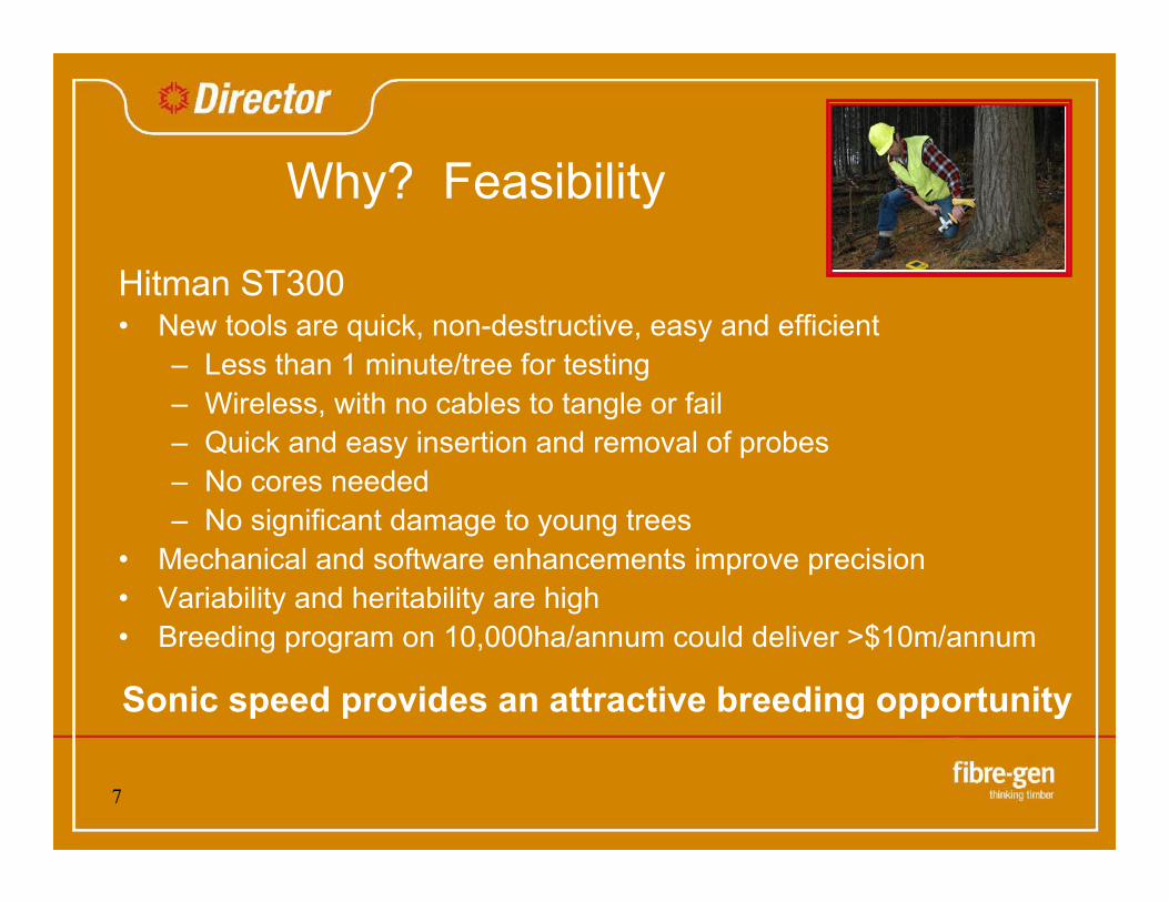
Why? Feasibility

Hitman ST300• New tools are quick, non-destructive, easy and efficient

– Less than 1 minute/tree for testing– Wireless, with no cables to tangle or fail– Quick and easy insertion and removal of probes– No cores needed– No significant damage to young trees

• Mechanical and software enhancements improve precision• Variability and heritability are high• Breeding program on 10,000ha/annum could deliver >$10m/annum

Sonic speed provides an attractive breeding opportunity

8

Why? Feasible and valuableHitman ST300• Variability and heritability are

high• Example mean 3.2 km/sec with

SD 0.2• Top 10% mean is 3.5 km/sec• Top 2% mean is 3.63km/sec• With heritability of 60%,

delivered gain is 0.18 and 0.26 respectively

• MSG example values this at $1,180 and $1,700/ha NPV at time of planting

Normal Distribution

0%2%4%6%8%

10%12%14%

2.6 2.7 2.8 2.9 3 3.1 3.2 3.3 3.4 3.5 3.6 3.7 3.8

Velocity (km/sec)

9

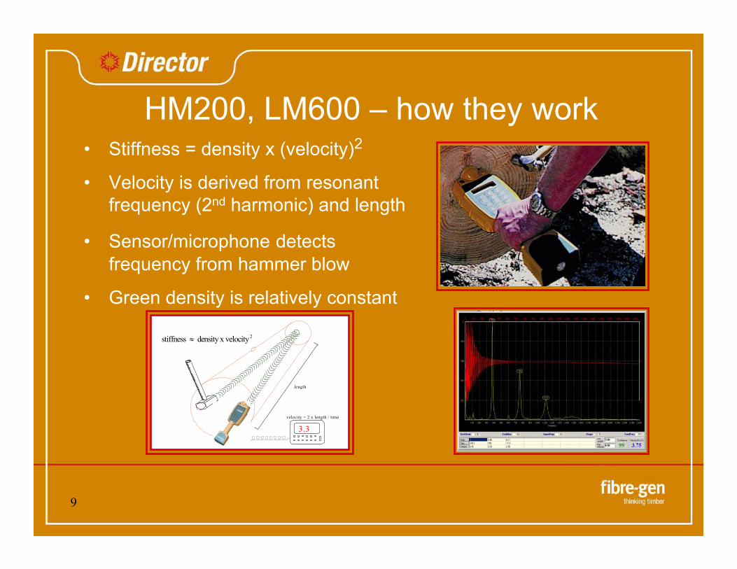
HM200, LM600 – how they work• Stiffness = density x (velocity)2

• Velocity is derived from resonant frequency (2nd harmonic) and length

• Sensor/microphone detects frequency from hammer blow

• Green density is relatively constant

3.3

length

velocity = 2 x length / time

stiffness density x velocity≈ 2

10

Hitman ST300, PH330 – how they work• ‘Time of flight’ outerwood velocity measure – higher than

log measure• Ruggedised, waterproof, wireless, auto-distance, audible

and visual output, interface to PDA• Velocity correlates strongly with log velocity at stand

levelAcoustic speed - standing tree vs log

6000

7000

8000

9000

10000

11000

12000

13000

14000

6000 8000 10000 12000 14000 16000

ST300 prototype on tree (ft/s)

HM

200

on lo

g (D

irect

or) (

ft/s)

Sitka spruceWestern hemlockJack pineWhite birchPonderosa pine

R2 = 0.925

Source: X Wang et al, University of Minnesota

Juvenile Wood

15 yrs 25 yrs 35 yrs

Juvenile Wood

15 yrs 25 yrs 35 yrs

11

Improved PrecisionHitman ST300• Mechanical and software enhancements improve

precision– Calibration against absolute standard– Filters enhance precision

TOF vs Distance (Brass Bar)

y = 0.2941x + 0.2476R2 = 0.9997

050

100150200250300350400450500

0 500 1000 1500

Distance (mm)

TOF

(us)

Recorded Time of Flight Variation(SD 3.5 vs 7.5)

300

320

340

360

380

400

420

440

460

480

500

1 2 3 4 5 6 7 8 9 10 11 12 13 14 15 16

Sample number

Tim

e of

Flig

ht (m

icro

-sec

)

12

Standing tree sampling – single trees• Measure is a single sample of outerwood velocity• Sampling procedure and intensity must match need• Single tree - intensive sampling

– Variation around stem– Knot location– Transverse – Compression wood– Hit variability

• 1-3 sets of 10 hits, in each of 2-4 locations around stem• High productivity (>60 sample sets/hour) – faster than

density coring

13

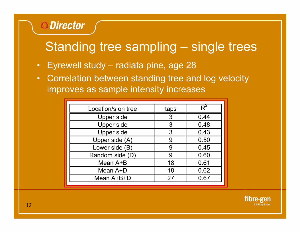
Standing tree sampling – single trees• Eyrewell study – radiata pine, age 28• Correlation between standing tree and log velocity

improves as sample intensity increases

Location/s on tree taps R2

Upper side 3 0.44Upper side 3 0.48Upper side 3 0.43

Upper side (A) 9 0.50Lower side (B) 9 0.45

Random side (D) 9 0.60Mean A+B 18 0.61Mean A+D 18 0.62

Mean A+B+D 27 0.67

14

Standing tree sampling – single trees

• Sawlog study –radiata pine

• Correlation between standing tree and log velocity improves as sample intensity increases

Correlation vs number of samples

0.00

0.20

0.40

0.60

0.80

1.00

0 10 20 30 40 50

Number of samples

Cor

rela

tion

(R2 )

Rx 0031Rx 0035

15

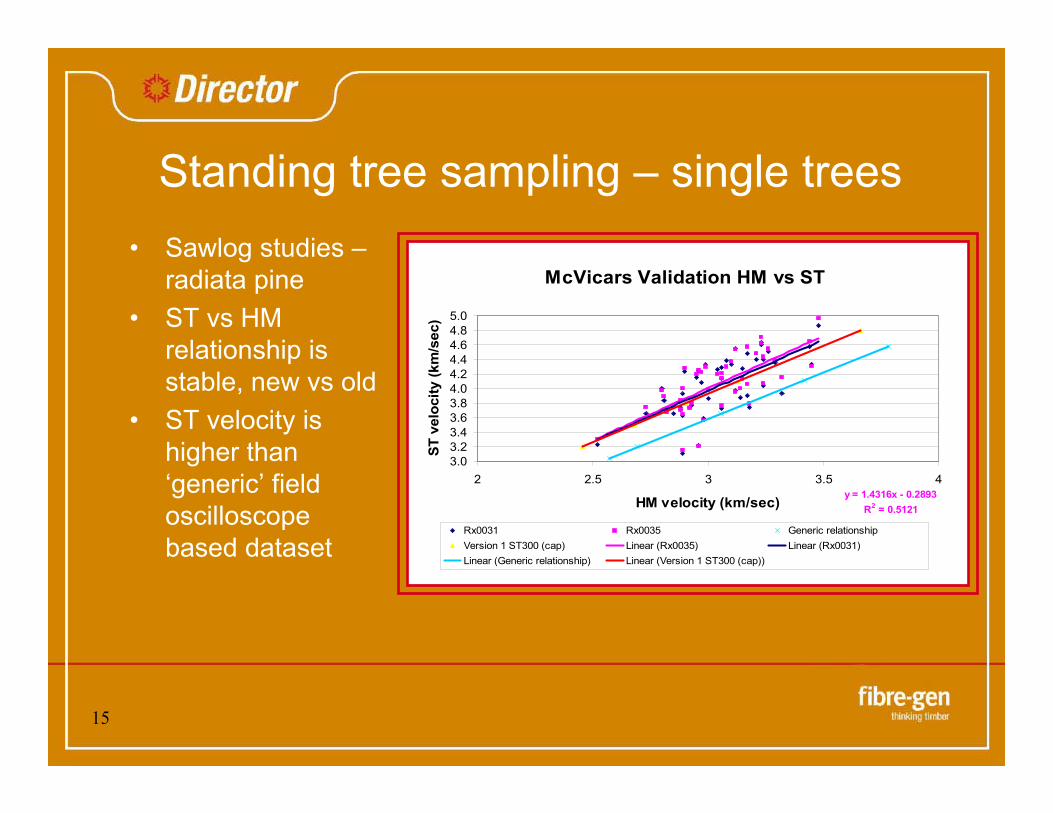
Standing tree sampling – single trees• Sawlog studies –

radiata pine• ST vs HM

relationship is stable, new vs old

• ST velocity is higher than ‘generic’ field oscilloscope based dataset

McVicars Validation HM vs ST

y = 1.4316x - 0.2893R2 = 0.5121

3.03.23.43.63.84.04.24.44.64.85.0

2 2.5 3 3.5 4

HM velocity (km/sec)

ST v

eloc

ity (k

m/s

ec)

Rx0031 Rx0035 Generic relationshipVersion 1 ST300 (cap) Linear (Rx0035) Linear (Rx0031)Linear (Generic relationship) Linear (Version 1 ST300 (cap))

16

Standing tree sampling - stands• More extensive sampling – large block genetic gain

trials• Stand average measure

– Cover the stand – plots of 5+ trees– Cover diameter range– Variability between trees > within– Sample as many trees as possible in least time

• 1 set of 10 hits/tree on 50+ trees/stand• Productivity dependent upon terrain and vegetation

17

Target Velocities – NZ example• Dynamic MOE of 8GPa is indicative of VSG8 production and

would require– Average log velocity 2.8km/sec (allowing 0.1km/sec for SE

of mean)– Green density 1000kg/m3

• 8GPa target velocity could vary 2.70 - 3.00 km/sec average

• Equivalent standing tree velocities 3.6 - 4.0 km/sec average at harvest

• Towards end of juvenile wood formation, target 2.8 km/sec although 2.6 may be adequate for structural minimum (5.6 GPa)

18

Results – effect of temperature on velocityIn general• Acoustic velocity is higher at lower temperaturesBut• Rate of change is most significant around freezing• Moisture content changes may compensate on logs, but not in trees

Temperature Effect on Acoustic Velocity of Green Board

0200400600800

1000120014001600180020002200240026002800300032003400360038004000

-20 -15 -10 -5 0 5 10 15 20

Board Temperature (C)

Aco

ustic

Wav

e Ve

loci

ty (m

/s)

Stack 6 (50 boards)Stack 2 (50 boards)

V = 2365 - 17.69T (T ? 0 °C)

V = 2365 - 41.42T (T ? 0 °C)

Density (MC) adjusted acoustic speed

2

2.5

3

3.5

4

4.5

5

-25 -20 -15 -10 -5 0 5 10 15 20 25

Series1Series2Series3Series4Series5Series6Series7Series8Series9Series10Series11Series12

Source: L Bjorklund, VMR, SDCSource: P Harris, IRLSource: X Wang, University of Minnesota

19

Results –velocity within stem – butt to top• Acoustic velocity varies from butt to top although

greatest variation is between stems• Highest velocity logs are in mid section of stem• Variation follows pattern of microfibril angle

Source: X Wang et al, University of Minnesota

Radiata Pine - Log velocity within stem

2.50

3.00

3.50

4.00

0 5 10 15 20 25 30

Distance up stem (m)

Velo

city

(km

/sec

)

Average 3.2 km/ secAverage + 2 x SDAverage - 2 x SDStand Mean 3.2

20

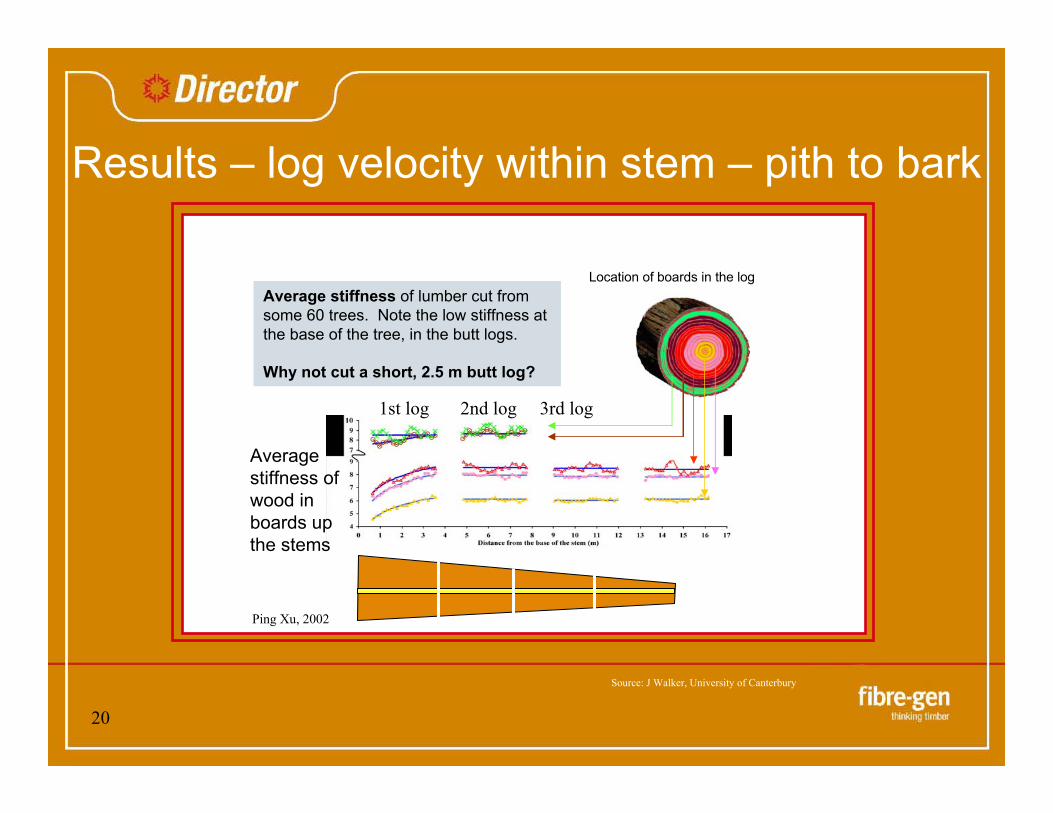
Location of boards in the log

Averagestiffness ofwood inboards upthe stems

Average stiffness of lumber cut from some 60 trees. Note the low stiffness at the base of the tree, in the butt logs.

Why not cut a short, 2.5 m butt log?

1st log 2nd log 3rd log

Ping Xu, 2002

Results – log velocity within stem – pith to bark

Source: J Walker, University of Canterbury

21

Results – velocity and MoE correlate with ageIn general• Acoustic velocity increases with increasing ageBut• Other factors affect velocity and MoE• Wide range of velocities within stands• Strategy – set appropriate breeding targets for different ages

Log age vs. average acoustic velocity

R2 = 0.66

2.50

2.60

2.70

2.80

2.90

3.00

3.10

3.20

3.30

3.40

3.50

18 20 22 24 26 28 30 32 34

Log age (years)

StandLinear (Stand)

Velocity vs Stand Age

2.80

2.90

3.00

3.10

3.20

3.30

3.40

3.50

3.60

3.70

20 21 22 23 24 25 26 27 28 29 30 31 32 33 34 35 36 37

Age (years)

Velo

city

(km

/sec

)Mean Velocity (50% oldest age) = 3.43Mean Velocity (50% highest V) = 3.37

Benefit = 0.06km/ sec

22

Conclusions• Highly significant values are at stake

• Variation and heritability are high

• New tools are available that are easy to use, efficient, and precise

• Breeding applications include clonal ranking, progeny trials, and genetic gain studies

• For supporting information

[email protected]

www.fibre-gen.com