Embed Size (px)
DESCRIPTION
Belgian Institute for Postal services and Telecommunications / Consultation document for the draft NGN/NGA models
Citation preview

Ref: 17915-516
BIPT‟s NGN/NGA model
Model version v1.0 documentation for industry players
Report for BIPT
23 December 2011
2
17915-516
Copyright © 2011. Analysys Mason Limited has produced the information
contained herein for BIPT. The ownership, use and disclosure of this information
are subject to the Commercial Terms contained in the contract between
Analysys Mason and BIPT

3
17915-516
Model overview
Market module
Ancillary/common/overhead modules
Access modules
Core modules
Service costing modules
Contents
Introduction
Glossary

4
17915-516
Context and objectives
Analysys Mason Limited („Analysys Mason‟) has been commissioned to assist BIPT in developing and
implementing a long-run incremental cost (LRIC) model for next-generation fixed networks in Belgium
The objectives of the project are to develop a bottom-up cost model of a next-generation core and
access (fixed) network to calculate the unit costs of the services provided on the network. The results of
the model will be used to:
develop business plans of generic Internet service providers (ISPs) to ensure the economic
viability of wholesale tariffs
determine appropriate tariffs for regulated fixed wholesale services (BRUO, BRIO, BROBA, etc.)
This document is the technical model documentation accompanying the draft models and presents how the
models work
It should be read in conjunction with:
the industry presentation „Draft NGN/NGA models‟ dated 13 December 2011 (ref. 17915-454), which
describes notably modelling principles, next steps and issues for consultation
the model content list „Bottom-up fixed network cost model for BIPT: list of model components –
public version‟, dated 13 December 2011 (ref. 17915-454)
the draft model consultation document, presented in English, French and Dutch versions, dated 13
December 2011 (ref: 17915-454)
Introduction
5
17915-516
Introduction
Model overview
Market module
Ancillary/common/overhead modules
Access modules
Core modules
Service costing modules
Glossary
6
17915-516
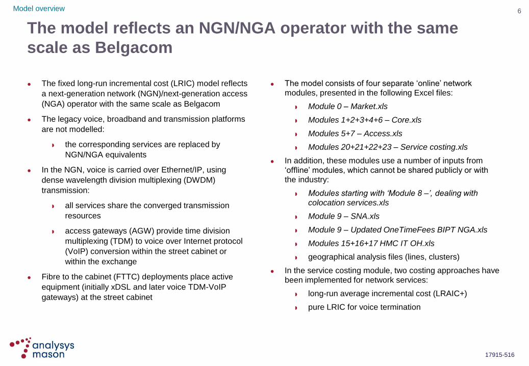
The model reflects an NGN/NGA operator with the same
scale as Belgacom
The fixed long-run incremental cost (LRIC) model reflects
a next-generation network (NGN)/next-generation access
(NGA) operator with the same scale as Belgacom
The legacy voice, broadband and transmission platforms
are not modelled:
the corresponding services are replaced by
NGN/NGA equivalents
In the NGN, voice is carried over Ethernet/IP, using
dense wavelength division multiplexing (DWDM)
transmission:
all services share the converged transmission
resources
access gateways (AGW) provide time division
multiplexing (TDM) to voice over Internet protocol
(VoIP) conversion within the street cabinet or
within the exchange
Fibre to the cabinet (FTTC) deployments place active
equipment (initially xDSL and later voice TDM-VoIP
gateways) at the street cabinet
The model consists of four separate „online‟ network modules, presented in the following Excel files:
Module 0 – Market.xls
Modules 1+2+3+4+6 – Core.xls
Modules 5+7 – Access.xls
Modules 20+21+22+23 – Service costing.xls
In addition, these modules use a number of inputs from „offline‟ modules, which cannot be shared publicly or with the industry:
Modules starting with ‘Module 8 –’, dealing with
colocation services.xls
Module 9 – SNA.xls
Module 9 – Updated OneTimeFees BIPT NGA.xls
Modules 15+16+17 HMC IT OH.xls
geographical analysis files (lines, clusters)
In the service costing module, two costing approaches have been implemented for network services:
long-run average incremental cost (LRAIC+)
pure LRIC for voice termination
Model overview

7
17915-516
Instructions on how to install and run the model
In order to run the model:
ensure that all network-related Excel files (Module 0 – Market.xls, Modules 1+2+3+4+6 – Core.xls,
Modules 5+7 – Access.xls and Modules 20+21+22+23 – Service costing.xls) are saved in the same
directory to preserve the inter-workbook links
open all four workbooks (in no particular order)
– when prompted to update the linked information, choose „No‟
– when asked whether or not to enable any macros, click the „Enable macros‟ box
check that all four workbooks are linked (using Edit Links menu)
the model should be used in „manual‟ calculation mode
To run the model under the various costing approaches, the macro must be used:
click the „Run pure LRIC and LRAIC+‟ macro button to run the model
the results of the model calculations can be viewed on the „Services needed‟ worksheet of the
Modules 20+21+22+23 - Service costing.xls workbook
Model overview

8
17915-516
All worksheets use a consistent cell format throughout
all four workbooks
This is to increase the transparency of the model, as well as making it easier to understand and modify
A number of standardised cell formats are used to distinguish inputs, assumptions, calculations and links.
The most important conventions are shown below
Cell type Cell style Notes
Input Parameter 100 An input to the model that it is expected the user will change (change at will)
Input Data 100 A piece of real data (only change if you have better data)
Input Estimate 100An estimate used in the absence of real data (only change if you have a better estimate, or
real data )
Input Calculation 100An input to the model that has, none the less, been calculated from other inputs (e.g.
interpolated input values)
Input Link 100An input to this part of the model, which is linked to a source on this or another worksheet
within this workbook
Input Link (different Workbook) 100An input to this part of the model, which is linked to a source on a worksheet in a different
workbook
Calculation 100 A calculation of the model
Total 123 A total (use if not part of a "Sub-total row" or a "Total row" in a table - see below)
Checksum 0.00A side calculation intended solely to cross check a result (and which therefore should not be
referenced anywhere else in the model)
Output 100A key result from this part of the model (in particular one that will be used elsewhere in the
model)
Named range NameAn Excel Name applying to one or more adjacent cells (use Insert Name Create to actually
create the Excel Names)
Note Note A note (NB smaller than standard font size)
Model overview
Anonymised Input 100 A rounded value used to protect the confidentiality of real data

9
17915-516
Model overview
Market module
Modelled operator
Market total
Overview
Core modules
Access modules
Service costing modules
Ancillary/common/overhead modules
Introduction
Glossary

10
17915-516
-
5
10
15
20
25
30
35
Min
ute
s (
bill
ion
)Mobile voice Fixed to fixed
Fixed to mobile Fixed to international
Fixed to non-geographic Fixed dial-up Internet
Evolution of traffic origination
The market module calculates market demand for both
fixed and mobile services
In the Belgian market:
traffic on fixed networks is declining
traffic on mobile networks is increasing
dial-up has disappeared almost completely
Market demand for both fixed and mobile services is
modelled based on data provided by BIPT‟s Market
Statistics and (confidential) information provided by
operators in response to the data request:
the data supplied by the operators is used to check
the validity of the public information and provide
other „average‟ parameters
The number of fixed subscribers in the market is
calculated using a projection of future population,
household and business penetration
The number of mobile subscribers used in the NGN-NGA
model is the same as in BIPT‟s latest mobile LRIC model
The forecast traffic demand is determined by a projection
of total voice origination, based on a long-term growth
driven by population growth assumptions
Source: BIPT model v1.0
Market module • Overview

11
17915-516
High-level flow of calculations in the market module
Market total Modelled operator
*Includes some data, at the total market level, from the mobile LRIC model †Total voice traffic means fixed and mobile, towards all recipients/destinations
Colour key Input Calculations Output
Penetration
forecast
Operator subscribers
forecast
Historical population/ household/ businesses
Market share
Total subscribers
forecast
Historical
penetration
Total historical
subscribers*
Population/ household/ business forecast
Total traffic forecast
Operator traffic
forecast
Total historical
voice traffic*
Traffic breakdown
forecast
Historical traffic breakdown
Historical
subscribers
Historical traffic Total voice
traffic forecast†
Historical traffic
per subscriber
(DSL and
IPTV)
Traffic per
subscriber
forecast (DSL
and IPTV)
Market module • Overview
12
17915-516
Model overview
Market module
Modelled operator
Market total
Overview
Core modules
Access modules
Service costing modules
Ancillary/common/overhead modules
Introduction
Glossary
13
17915-516
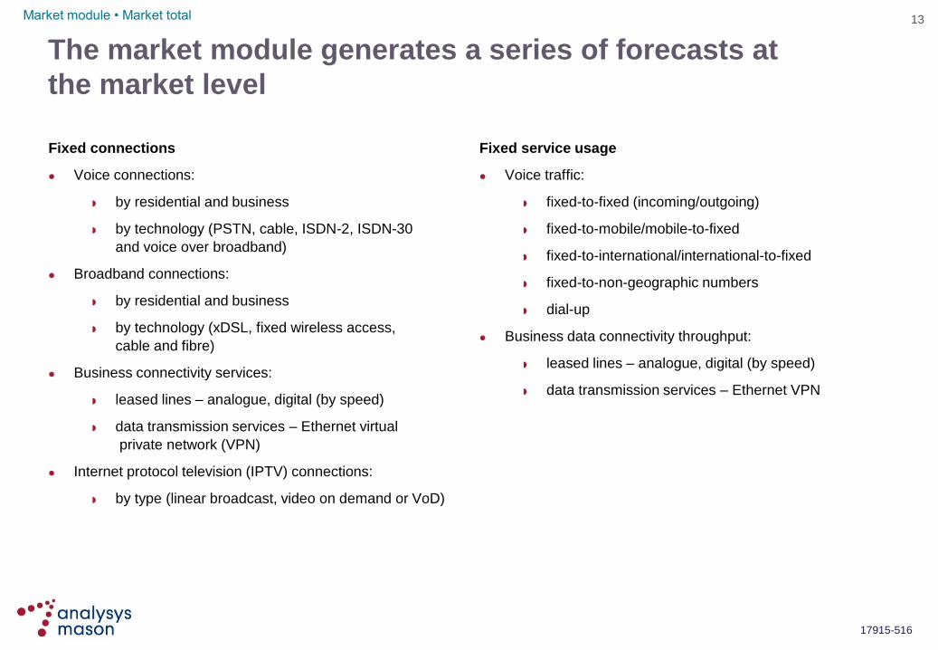
The market module generates a series of forecasts at
the market level
Fixed connections
Voice connections:
by residential and business
by technology (PSTN, cable, ISDN-2, ISDN-30
and voice over broadband)
Broadband connections:
by residential and business
by technology (xDSL, fixed wireless access,
cable and fibre)
Business connectivity services:
leased lines – analogue, digital (by speed)
data transmission services – Ethernet virtual
private network (VPN)
Internet protocol television (IPTV) connections:
by type (linear broadcast, video on demand or VoD)
Fixed service usage
Voice traffic:
fixed-to-fixed (incoming/outgoing)
fixed-to-mobile/mobile-to-fixed
fixed-to-international/international-to-fixed
fixed-to-non-geographic numbers
dial-up
Business data connectivity throughput:
leased lines – analogue, digital (by speed)
data transmission services – Ethernet VPN
Market module • Market total

14
17915-516
Voice connections
Mobile voice connections
The number of mobile subscribers used in the NGN-NGA model is the same as in BIPT‟s latest mobile LRIC model
Fixed voice connections – residential
The number of residential fixed voice connections is driven by the number of households in Belgium
We have extrapolated the growth of household and fixed voice household penetration to forecast the number of residential fixed voice connections
This market is further split in five different fixed voice technologies: PSTN, cable, ISDN-2, ISDN-30 and VoB. The technology shares are extrapolated from the historical figures
Fixed voice connections – business
The number of business fixed voice connections is directly related to number of business sites in Belgium
Similar to its residential counterpart, the number of business fixed voice connections is forecast by extrapolating the growth of the number of business sites and fixed voice business penetration
This market is also split into the five aforementioned fixed voice technologies
Residential fixed
voice connection
(historical)
Household
forecast
Business fixed
voice connection
(historical)
Business sites
forecast
Residential fixed
voice penetration
(historical)
No. of fixed voice
connections per
business site
(historical)
Residential fixed
voice penetration
(forecast)
Residential
fixed voice by
technology
(historical)
Business
fixed voice by
technology
(historical)
Technology share
(historical)
Technology share
(historical)
Technology share
(forecast)
Technology share
(forecast)
Residential fixed
voice
connections by
technology
Business fixed
voice
connections
by technology
Total fixed voice
connections by
technology
Voice connection forecasts
No. of fixed voice
connections per
business site
(forecast)
Market module • Market total
Mobile voice
connections
Residential fixed
voice connection
(M-LRIC)
Colour key Input Calculations Output
15
17915-516
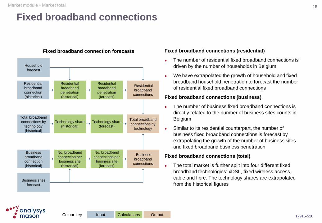
Fixed broadband connections
Fixed broadband connections (residential)
The number of residential fixed broadband connections is
driven by the number of households in Belgium
We have extrapolated the growth of household and fixed
broadband household penetration to forecast the number
of residential fixed broadband connections
Fixed broadband connections (business)
The number of business fixed broadband connections is
directly related to the number of business sites counts in
Belgium
Similar to its residential counterpart, the number of
business fixed broadband connections is forecast by
extrapolating the growth of the number of business sites
and fixed broadband business penetration
Fixed broadband connections (total)
The total market is further split into four different fixed
broadband technologies: xDSL, fixed wireless access,
cable and fibre. The technology shares are extrapolated
from the historical figures
Residential
broadband
connection
(historical)
Household
forecast
Business
broadband
connection
(historical)
Business sites
forecast
Residential
broadband
penetration
(historical)
No. broadband
connection per
business site
(historical)
No. broadband
connections per
business site
(forecast)
Residential
broadband
penetration
(forecast)
Total broadband
connections by
technology
(historical)
Technology share
(historical)
Technology share
(forecast)
Residential
broadband
connections
Business
broadband
connections
Fixed broadband connection forecasts
Total broadband
connections by
technology
Market module • Market total
Colour key Input Calculations Output
16
17915-516
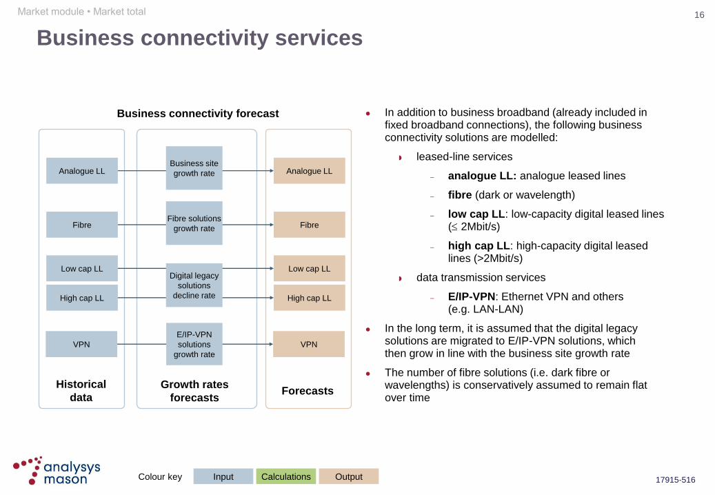
Business connectivity services
In addition to business broadband (already included in fixed broadband connections), the following business connectivity solutions are modelled:
leased-line services
– analogue LL: analogue leased lines
– fibre (dark or wavelength)
– low cap LL: low-capacity digital leased lines ( 2Mbit/s)
– high cap LL: high-capacity digital leased lines (>2Mbit/s)
data transmission services
– E/IP-VPN: Ethernet VPN and others (e.g. LAN-LAN)
In the long term, it is assumed that the digital legacy solutions are migrated to E/IP-VPN solutions, which then grow in line with the business site growth rate
The number of fibre solutions (i.e. dark fibre or wavelengths) is conservatively assumed to remain flat over time
Analogue LL
Low cap LL
High cap LL
VPN
Analogue LL
Low cap LL
High cap LL
VPN
Digital legacy
solutions
decline rate
E/IP-VPN
solutions
growth rate
Historical
data Forecasts
Growth rates
forecasts
Business connectivity forecast
Market module • Market total
Fibre Fibre
Business site
growth rate
Fibre solutions
growth rate
Colour key Input Calculations Output
17
17915-516
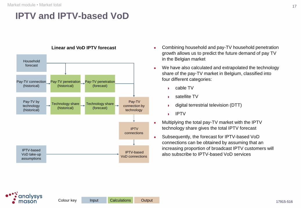
IPTV and IPTV-based VoD
Combining household and pay-TV household penetration
growth allows us to predict the future demand of pay TV
in the Belgian market
We have also calculated and extrapolated the technology
share of the pay-TV market in Belgium, classified into
four different categories:
cable TV
satellite TV
digital terrestrial television (DTT)
IPTV
Multiplying the total pay-TV market with the IPTV
technology share gives the total IPTV forecast
Subsequently, the forecast for IPTV-based VoD
connections can be obtained by assuming that an
increasing proportion of broadcast IPTV customers will
also subscribe to IPTV-based VoD services
Pay-TV connection
(historical)
Household
forecast
Pay-TV penetration
(historical)
Pay-TV penetration
(forecast)
Pay-TV by
technology
(historical)
Technology share
(historical)
Technology share
(forecast)
Pay-TV
connection by
technology
IPTV
connections
IPTV-based
VoD connections
IPTV-based
VoD take-up
assumptions
Linear and VoD IPTV forecast
Market module • Market total
Colour key Input Calculations Output
18
17915-516
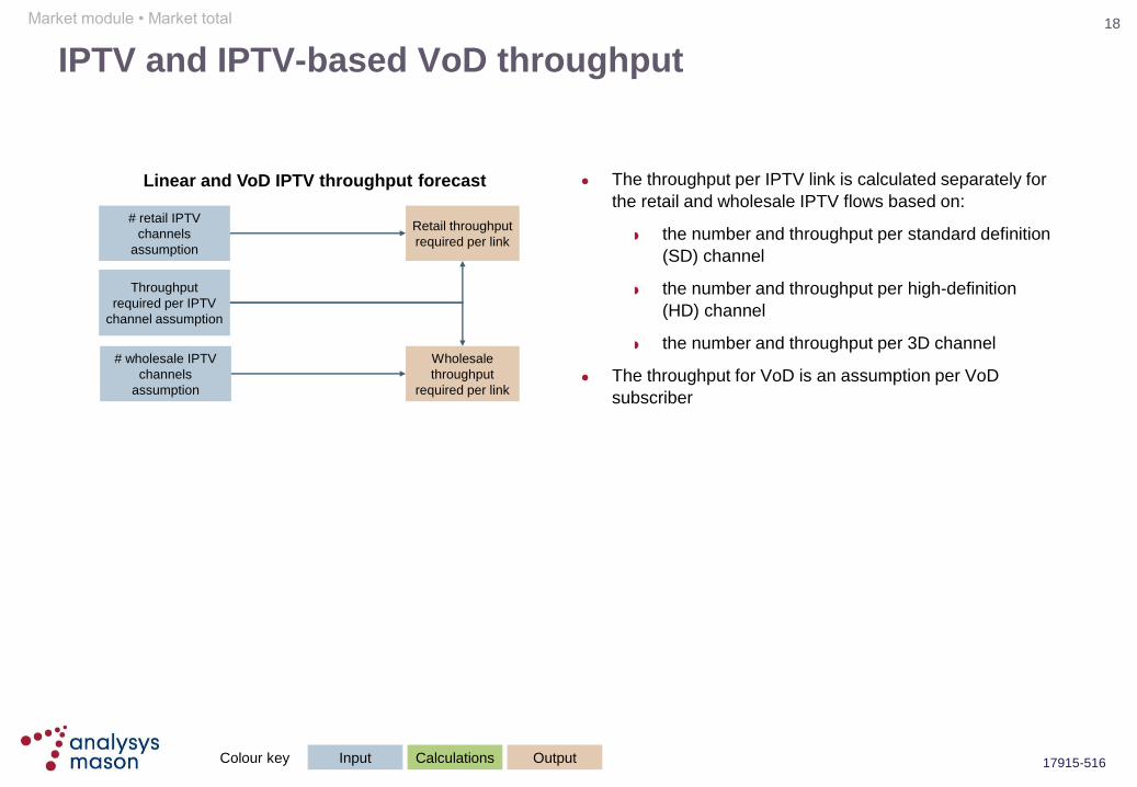
IPTV and IPTV-based VoD throughput
The throughput per IPTV link is calculated separately for
the retail and wholesale IPTV flows based on:
the number and throughput per standard definition
(SD) channel
the number and throughput per high-definition
(HD) channel
the number and throughput per 3D channel
The throughput for VoD is an assumption per VoD
subscriber
Linear and VoD IPTV throughput forecast
# retail IPTV
channels
assumption
Throughput
required per IPTV
channel assumption
Retail throughput
required per link
# wholesale IPTV
channels
assumption
Wholesale
throughput
required per link
Market module • Market total
Colour key Input Calculations Output

19
17915-516
Mobile voice
connection as %
total voice connection
FTM as % FTN traffic
(forecast)
Preference coefficient
(historical + forecast)
FTM as % FTN traffic
(historical)
FTF&NG as % FTN
traffic (forecast)
FTF&NG as % FTN
traffic (historical)
FTI as % fixed
originated traffic
(historical)
FTI as % fixed
originated traffic
(forecast)
FTI traffic (forecast)
FTF traffic (forecast)
FTNG traffic
(forecast) Fixed
origination
FTNG as % FTF&NG
traffic (historical)
FTM traffic (forecast)
FTNG as % FTF&NG
traffic (forecast)
Voice traffic forecasts at a glance
In the flow chart:
FTI = fixed to international
FTN = fixed to national
FTM = fixed to mobile
FTF&NG = fixed to fixed and non-
geographic numbers
FTF = fixed to fixed
FTNG = fixed to non-geographic
numbers
MTI = mobile to international
MTN = mobile to national
MTM = mobile to mobile
MTF = mobile to fixed
ITF = international to fixed
Total voice originated
traffic (historical)
Total voice originated
traffic (forecast)
% being mobile
originated (historical)
% being mobile
originated (forecast)
Mobile originated
traffic (historical)
Fixed originated
traffic (historical)
Fixed dial-up Internet
traffic (historical)
Mobile originated
traffic (forecast)
Fixed originated
traffic (forecast)
Fixed dial-up Internet
traffic (forecast)
Mobile voice
connection as % total
voice connection
MTM as % MTN
traffic (forecast)
Preference coefficient
(historical + forecast)
MTM as % MTN
traffic (historical)
MTF as % MTN traffic
(forecast)
MTF as % MTN traffic
(historical)
MTI as % mobile
originated traffic
(historical)
MTI as % mobile
originated traffic
(forecast)
MTI traffic (forecast)
MTM traffic (forecast)
MTF traffic (forecast)
Mobile
origination
Details on the flow of
calculations are provided
in the following four slides
Market module • Market total
ITF traffic (forecast)
International traffic
imbalance
assumptions
FTF terminated traffic
(forecast)
MTF traffic (forecast)
FTF terminated traffic
as % of FTF
originated traffic
Fixed
termination
Colour key Input Calculations Output

20
17915-516
Firstly, the origination traffic is split into three broad
categories BIPT provides historical data for the
fixed to non-geographic traffic (used
to estimate historical dial-up Internet
traffic), fixed- and mobile-originated
traffic
We have extrapolated the sum of
these traffic categories, as well as
the share of mobile-originated traffic
Multiplying these gives the forecast of
mobile-originated traffic
We have projected the dial-up Internet
traffic directly to reflect the diminishing
use of this service
Fixed-originated traffic can be
obtained by subtracting away the
mobile-originated traffic from the total
traffic (as the dial-up Internet traffic is
assumed to go down to 0 from 2009)
Total voice originated
traffic (historical)
Total voice originated
traffic (forecast)
% being mobile
originated (historical)
% being mobile
originated (forecast)
Mobile originated
traffic (historical)
Fixed originated
traffic (historical)
Fixed dial-up Internet
traffic (historical)
Mobile originated
traffic (forecast)
Fixed originated
traffic (forecast)
Fixed dial-up Internet
traffic (forecast)
Fixed
origination
Mobile
origination
Fixed
termination
Market module • Market total
Colour key Input Calculations Output

21
17915-516
Next, the fixed-originated traffic is further split into
smaller sub-categories FTM, FTF&NG and FTI traffic shares
are forecast as percentages of the total
fixed-originated traffic:
the fixed-originated traffic is first
split into FTI and FTN traffic
FTN traffic is then further split
into FTF&NG and FTM traffic
FTF&NG is then further split into
FTF and FTNG
The split between FTF and FTM traffic
is directly related to the split between
fixed and mobile connections
However, the correlation is not perfect –
fixed users are more likely to call a fixed
telephone than a mobile telephone.
Hence, a „preference coefficient‟* is
defined to capture this effect
Multiplying these traffic shares with the
total fixed-originated traffic obtained
earlier gives the FTM, FTF, FTNG and
FTI traffic forecasts
Total voice originated
traffic (historical)
Total voice originated
traffic (forecast)
% being mobile
originated (historical)
% being mobile
originated (forecast)
Mobile originated
traffic (historical)
Fixed originated
traffic (historical)
Fixed dial-up Internet
traffic (historical)
Mobile originated
traffic (forecast)
Fixed originated
traffic (forecast)
Fixed dial-up Internet
traffic (forecast)
Mobile voice
connection as % total
voice connection
FTM as % FTN traffic
(forecast)
Preference coefficient
(historical + forecast)
FTM as % FTN traffic
(historical)
FTF&NG as % FTN
traffic (forecast)
FTF&NG as % FTN
traffic (historical)
FTI as % fixed
originated traffic
(historical)
FTI as % fixed
originated traffic
(forecast)
FTI traffic (forecast)
FTF traffic (forecast)
FTNG traffic
(forecast) Fixed
origination
Mobile
origination
Fixed
termination
*The ‘preference coefficient’ for FTM calls is defined as the
ratio of ‘FTM calls as a percentage of FTN calls’ to ‘mobile
connections as a percentage of voice connections’
Market module • Market total
FTNG as % FTF&NG
traffic (historical)
FTM traffic (forecast)
FTNG as % FTF&NG
traffic (forecast)
Colour key Input Calculations Output

22
17915-516
A similar sub-categorisation is performed on the mobile-
originated traffic
Total voice originated
traffic (historical)
Total voice originated
traffic (forecast)
% being mobile
originated (historical)
% being mobile
originated (forecast)
Mobile originated
traffic (historical)
Fixed originated
traffic (historical)
Fixed dial-up Internet
traffic (historical)
Mobile originated
traffic (forecast)
Fixed originated
traffic (forecast)
Fixed dial-up Internet
traffic (forecast)
Mobile voice
connection as % total
voice connection
MTM as % MTN
traffic (forecast)
Preference coefficient
(historical + forecast)
MTM as % FTN traffic
(historical)
MTF as % MTN traffic
(forecast)
MTF as % FTN traffic
(historical)
MTI as % mobile
originated traffic
(historical)
MTI as % mobile
originated traffic
(forecast)
MTI traffic (forecast)
MTM traffic (forecast)
MTF traffic (forecast)
Fixed
origination
Mobile
origination
Fixed
termination
MTM, MTF and MTI traffic shares are
forecast as percentages of the total
mobile-originated traffic:
the mobile-originated traffic is
first split into MTI and MTN
traffic
MTN traffic is then further split
into MTF and MTM traffic
The split between MTF and MTM
traffic is directly related to the split
between fixed and mobile connections
However, the correlation is not perfect
– mobile users are more likely to call a
mobile rather than a fixed telephone.
Hence, a „preference coefficient‟ is
defined to capture this effect
Multiplying these traffic shares with the
total mobile-originated traffic obtained
earlier gives the MTM, MTF and MTI
traffic forecasts
Market module • Market total
Colour key Input Calculations Output

23
17915-516
ITF traffic (forecast)
Finally, the relevant origination traffic is collected to
forecast the fixed-terminated traffic Three types of traffic generate fixed
termination: FTF, ITF and MTF
FTF-terminated traffic is forecast
based on FTF-originated traffic and
the share of FTF terminated as a
proportion of FTF-originated traffic
(excluding on-net traffic)
ITF and FTI traffic are correlated –
people who frequently make
international calls are also more
likely to receive calls from foreign
destinations
Hence, an „international traffic
imbalance‟ factor, defined as the
ratio of ITF-to-FTI traffic, is
assumed to estimate ITF traffic from
the FTI traffic determined earlier
MTF traffic is taken directly from
previous mobile-originated forecasts
Total voice originated
traffic (historical)
Total voice originated
traffic (forecast)
% being mobile
originated (historical)
% being mobile
originated (forecast)
Mobile originated
traffic (historical)
Fixed originated
traffic (historical)
Fixed dial-up Internet
traffic (historical)
Mobile originated
traffic (forecast)
Fixed originated
traffic (forecast)
Fixed dial-up Internet
traffic (forecast)
FTI traffic (forecast)
FTF traffic (forecast)
MTF traffic (forecast)
Fixed
origination
Mobile
origination
International traffic
imbalance
assumptions
FTF terminated traffic
(forecast)
MTF traffic (forecast)
FTF terminated traffic
as % of FTF
originated traffic
Fixed
termination
Market module • Market total
Colour key Input Calculations Output
24
17915-516
Model overview
Market module
Modelled operator
Market total
Overview
Core modules
Access modules
Service costing modules
Ancillary/common/overhead modules
Introduction
Glossary
25
17915-516
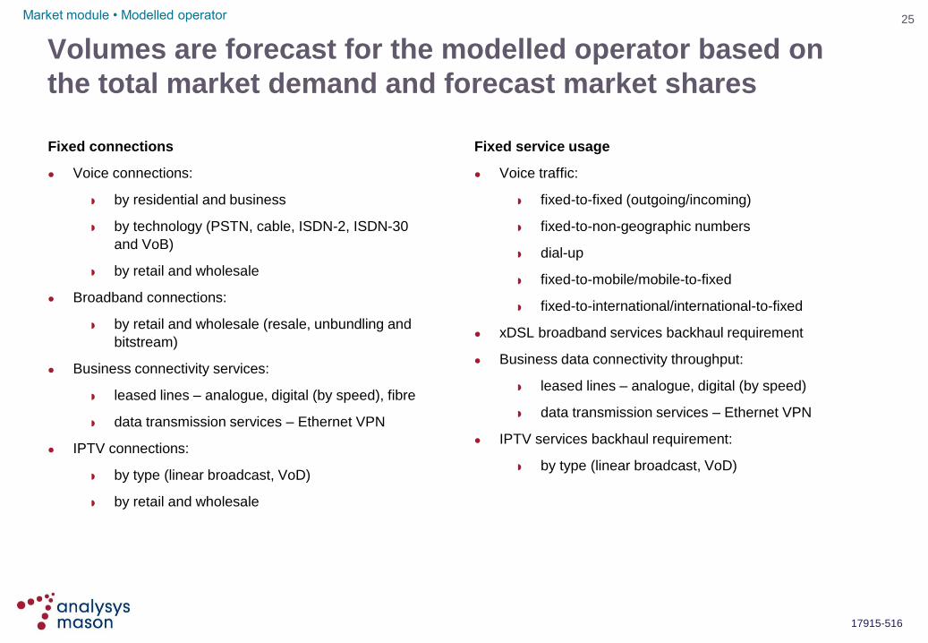
Volumes are forecast for the modelled operator based on
the total market demand and forecast market shares
Fixed connections
Voice connections:
by residential and business
by technology (PSTN, cable, ISDN-2, ISDN-30
and VoB)
by retail and wholesale
Broadband connections:
by retail and wholesale (resale, unbundling and
bitstream)
Business connectivity services:
leased lines – analogue, digital (by speed), fibre
data transmission services – Ethernet VPN
IPTV connections:
by type (linear broadcast, VoD)
by retail and wholesale
Fixed service usage
Voice traffic:
fixed-to-fixed (outgoing/incoming)
fixed-to-non-geographic numbers
dial-up
fixed-to-mobile/mobile-to-fixed
fixed-to-international/international-to-fixed
xDSL broadband services backhaul requirement
Business data connectivity throughput:
leased lines – analogue, digital (by speed)
data transmission services – Ethernet VPN
IPTV services backhaul requirement:
by type (linear broadcast, VoD)
Market module • Modelled operator

26
17915-516
Market total fixed voice connections are split between
the modelled operator and other operators
The market total number of fixed voice
connections needs to be split into connections
provided by the modelled operator and
connections provided by other operators
This is done based on the market share (by
technology) of:
retail other operators within the total
market
self-supply other operators within the retail
other operators
These calculations give the number of retail and
wholesale access lines for the modelled
operator, which added up yield the total number
of access lines (by technology) for the modelled
operator
Re-categorisation of fixed voice connections
Fixed voice
connections by
technology
(historical +
forecast)
Retail other
operators access
lines by technology
Market share of
retail other
operators by
technology
Market share of
self-supply other
operators within
retail other
operators by
technology
Self-supply other
operators access
lines by technology
Modelled
operator
(wholesale)
access lines
by technology
Modelled
operator (retail)
access lines by
technology
Modelled
operator
residential
access lines by
technology
Residential
Business
Similar calculations
Modelled
operator
business access
lines by
technology
Modelled
operator voice
connections by
technology
Market module • Modelled operator
Colour key Input Calculations Output
27
17915-516
xDSL broadband
connections
(historic +
forecast)
Retail other
operators
broadband
connections
Market share of
retail other
operators
Market share of
each
procurement
type within retail
other operators
Broadband
connections by
procurement type
for retail other
operators
Modelled operator
(retail) broadband
connections
Modelled operator
broadband
connections by
procurement type
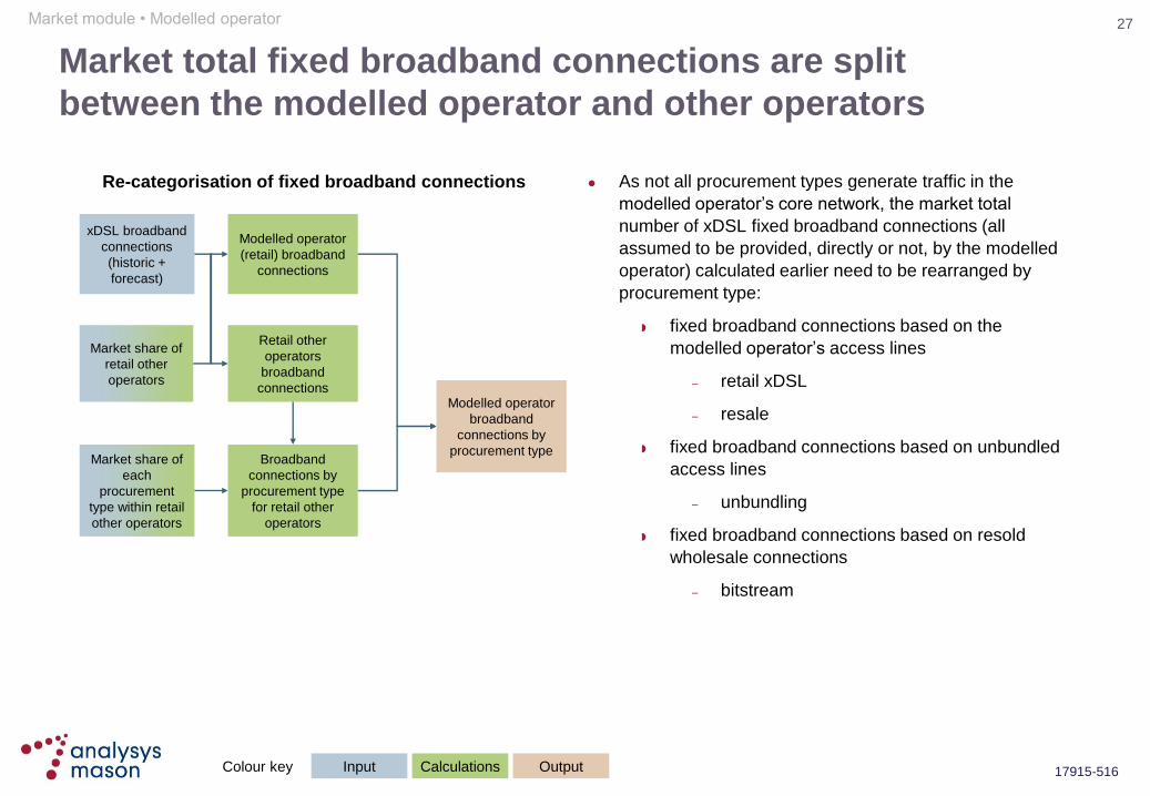
Market total fixed broadband connections are split
between the modelled operator and other operators
As not all procurement types generate traffic in the
modelled operator‟s core network, the market total
number of xDSL fixed broadband connections (all
assumed to be provided, directly or not, by the modelled
operator) calculated earlier need to be rearranged by
procurement type:
fixed broadband connections based on the
modelled operator‟s access lines
– retail xDSL
– resale
fixed broadband connections based on unbundled
access lines
– unbundling
fixed broadband connections based on resold
wholesale connections
– bitstream
Re-categorisation of fixed broadband connections
Market module • Modelled operator
Colour key Input Calculations Output
28
17915-516
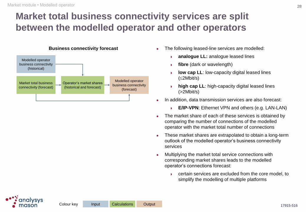
Market total business connectivity services are split
between the modelled operator and other operators
The following leased-line services are modelled:
analogue LL: analogue leased lines
fibre (dark or wavelength)
low cap LL: low-capacity digital leased lines
(2Mbit/s)
high cap LL: high-capacity digital leased lines
(>2Mbit/s)
In addition, data transmission services are also forecast:
E/IP-VPN: Ethernet VPN and others (e.g. LAN-LAN)
The market share of each of these services is obtained by
comparing the number of connections of the modelled
operator with the market total number of connections
These market shares are extrapolated to obtain a long-term
outlook of the modelled operator‟s business connectivity
services
Multiplying the market total service connections with
corresponding market shares leads to the modelled
operator‟s connections forecast:
certain services are excluded from the core model, to
simplify the modelling of multiple platforms
Operator‟s market shares
(historical and forecast)
Modelled operator
business connectivity
(historical)
Market total business
connectivity (forecast)
Modelled operator
business connectivity
(forecast)
Business connectivity forecast
Market module • Modelled operator
Colour key Input Calculations Output

29
17915-516
IPTV connections and IPTV-based VoD throughput are
split between the modelled operator and other operators
The number of retail and wholesale IPTV connections for
the modelled operator is driven by:
the total IPTV market connections
the share of each type of subscribers
The throughput required for retail and wholesale VoD is
driven by:
the number of retail and wholesale IPTV
subscribers
the share of VoD users among IPTV subscribers
the throughput required per VoD user
Market total number
of IPTV connections
Modelled operator‟s
retail vs. wholesale
market share of IPTV
connections
Modelled operator‟s
IPTV retail and
wholesale
connections
Modelled operator‟s
VoD retail and
wholesale
connections
Throughput
required per VoD
subscriber
assumption
Total throughput
required for retail
and wholesale VoD
IPTV connections forecast
Share of IPTV
subscribers who are
also VoD users
Market module • Modelled operator
Colour key Input Calculations Output

30
17915-516
Retail and wholesale origination voice traffic is derived
from the number of retail and wholesale subscribers
An operator‟s traffic market share correlates strongly with
its subscriber market share
However, subscribers‟ usage patterns differ by operator
and by call type. Hence, „usage coefficients‟ are
introduced to ensure the traffic market shares can be
predicted accurately from the subscribers market shares:
an operator‟s usage coefficient of a particular retail
origination service is defined as the ratio of its
market share for that particular service to its
market share of the retail fixed connections
We have derived and forecast the usage coefficients
using the modelled operator‟s shares of traffic and
connections
Multiplying these coefficients with the number of the
operator‟s retail/wholesale fixed connections leads to the
operator‟s retail/wholesale traffic forecast by origination
type
Retail and wholesale origination forecast
Retail usage
coefficient (historical
and forecast)
Other operators self-supply
vs wholesale modelled
operator traffic as % of
retail other operators by
origination type
Modelled operator
retail traffic by
origination type as
% of total (historical)
Other operators self-
supply vs wholesale
modelled operator
connections as % of
retail other operators
Modelled operator
retail traffic by
origination type
(historical)
Modelled operator
retail connections as
% of total
Modelled operator
retail traffic by
origination type
(forecast)
Modelled operator
wholesale
origination traffic
(forecast)
Market total retail
traffic by origination
type (historical
and forecast)
Other operators retail
traffic by origination
type (historical
and forecast)
Modelled operator
retail traffic by
origination type as %
of total (forecast)
Market module • Modelled operator
Colour key Input Calculations Output

31
17915-516
Wholesale transit voice traffic is modelled as a share of all
other traffic types
Wholesale transit services are generated by other
operators using the modelled operator‟s network. It can
be modelled as a share of the market services that can
generate transit traffic. These relevant services are:
fixed to fixed (ordinary numbers)
fixed to non-geographic numbers
dial-up Internet
fixed to mobile
fixed to international
mobile to fixed
international to fixed
mobile to mobile (off-net)
mobile to international
international to mobile
An extrapolation of the split between the regional and
national transit traffic leads to a forecast of these two
types of transit traffic
Share of the relevant
services which use transit
(historical and forecast)
Market total
transit traffic
(historical)
Market total
traffic of the
relevant services
(historical and
forecast)
Market total
transit traffic
(forecast)
Split between
regional and
national transit
traffic (historical
and forecast)
Wholesale transit traffic forecast
Modelled
operator transit
traffic (historical)
Share of transit
of the modelled
operator
(historical and
forecast)
Modelled
operator transit
traffic (forecast)
Modelled
operator regional
and national
transit traffic
(historical and
forecast)
Market module • Modelled operator
Colour key Input Calculations Output
32
17915-516
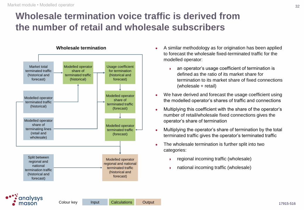
Wholesale termination voice traffic is derived from
the number of retail and wholesale subscribers
A similar methodology as for origination has been applied
to forecast the wholesale fixed-terminated traffic for the
modelled operator:
an operator‟s usage coefficient of termination is
defined as the ratio of its market share for
termination to its market share of fixed connections
(wholesale + retail)
We have derived and forecast the usage coefficient using
the modelled operator‟s shares of traffic and connections
Multiplying this coefficient with the share of the operator‟s
number of retail/wholesale fixed connections gives the
operator‟s share of termination
Multiplying the operator‟s share of termination by the total
terminated traffic gives the operator‟s terminated traffic
The wholesale termination is further split into two
categories:
regional incoming traffic (wholesale)
national incoming traffic (wholesale)
Market total
terminated traffic
(historical and
forecast)
Wholesale termination
Modelled operator
share of
terminating lines
(retail and
wholesale)
Modelled operator
regional and national
terminated traffic
(historical and
forecast)
Modelled operator
terminated traffic
(historical)
Split between
regional and
national
termination traffic
(historical and
forecast)
Modelled operator
share of
terminated traffic
(forecast)
Modelled operator
share of
terminated traffic
(historical)
Usage coefficient
for termination
(historical and
forecast)
Modelled operator
terminated traffic
(forecast)
Market module • Modelled operator
Colour key Input Calculations Output

33
17915-516
xDSL data backhaul is forecast based on historical trends
The data backhaul per subscriber is forecast using an
S-curve
The data backhaul per subscriber is then multiplied by the
number of broadband connections to obtain the total data
backhaul by procurement type:
retail + resale and bitstream connections create a
data backhaul need for the modelled operator
unbundling connections generate traffic carried by
another operator and therefore do not create any
data backhaul need for the modelled operator
Broadband data backhaul
Data backhaul per
subscriber
(historical and
forecast)
Broadband
connections by
procurement type
Data backhaul by
procurement type
Market module • Modelled operator
Colour key Input Calculations Output

34
17915-516
Model overview
Market module
NGN data connectivity
Overview
Core modules
Access modules
Service costing modules
Ancillary/common/overhead modules
Demand conversion
NGN voice connectivity
Ethernet/IP core Service platforms
Introduction
Glossary

35
17915-516
High-level flow of calculations in the core module
Colour key Input „Active‟
calculation Output/result
„Offline‟
calculation
Core modules • Overview
Market module
Core module
Service costing
module Demand
volumes
Network
costs
Route sharing
analysis
Unit costs
Routeing
factors
Core asset
dimensioning
Core network
expenditures
Service unit
costs
Economic
depreciation
Core network
assumptions
Core network
geodata

36
17915-516
SB-REM
The model assumes that an IP network is deployed to
support all data traffic (xDSL, VPNs and IPTV) …
A mix of disaggregated/monolithic IP DSLAMs is deployed in the street cabinets (remote optical platform or
ROP)/local exchanges (LEX)-local distribution cabinets (LDC), respectively:
the DSLAMs deployed use IP rather than ATM for backhaul, under modern equivalent asset (MEA)
principles
Ethernet switches are deployed in the LEX and connect the DSLAMs to the core network
Service
router
Ethernet switch
Ethernet transport Service/control platforms
LAN switches
Business
access
High-level IP core network architecture diagram
Core modules • Overview
SB-REM
SB-REM
SB-REM
SR
Aggregator
IP-DSLAM
Ethernet cluster
Data connectivity
RADIUS
DNS
BRAS

37
17915-516
… and is upgraded to support NGN voice services
SBC Is used to police the IP connection between an external network and the call server controlled core voice network
CS Handles the call control while the IP network handles the user traffic
TGW Translates the TDM-based voice coming from TDM voice networks to IP for transit over the NGN core, used for SS7 interconnection
PR Provides routing to/from another NGN voice core, used for SIP interconnection
High-level NGN core network architecture diagram
AGW
Service
router
Ethernet switch
Ethernet transport Service/control platforms
PR PoI
TGW
SBC
CS
LAN switches
AGW
AGW
AGW
SR
Aggregator
LN-AGW
Ethernet
cluster
Data connectivity
AGW Provides PSTN port interface – in the street cabinets (ROP) or in the LEX/LDC – and translates TDM-based voice into VoIP
Core modules • Overview

38
17915-516
There are three types of nodes in the core network
The local exchanges (LEX) are made of three types of nodes:
service nodes and central service nodes (SN/CSN) – two CSN in Brussels and eight SN in Gent,
Antwerp, Liège and Charleroi (two in each location) are the main nodes in the modelled operator‟s
core network. They are linked by two core express rings
aggregation nodes (AN) are points where the wavelengths of one or more clusters are aggregated
before being sent to the SN/CSN. They are located on one of four core rings, ending at two SN
– there are 32 aggregation nodes in the modelled operator‟s core network
local nodes (LN) are all other LEX
– there are 552 local nodes in the modelled operator‟s core network
Core modules • Overview

39
17915-516
Map of SC geotypes
Street cabinets (SC)
Street cabinets are the aggregation points closest to the
customers. They define the boundary between the core
and access networks
Street cabinets are divided in five geotypes, based on
their size (number of active lines) and whether they were
already upgraded to ROP in 2008 (year for which the
latest BRUO/BROBA model could provide this
distinction). The five geotypes are as follows:
Source: Analysys Mason geo-analysis based on BRUO/BROBA model
S0 (Not VDSL eligible yet in 2008)
S1 (< 80 active lines)
S2 (≤ 180 active lines)
S3 (> 180 active lines)
S0+ (S0 in 2008, migrated at a later date to VDSL)
0
2,896
12,771
5,149
7,543
Core modules • Overview
40
17915-516
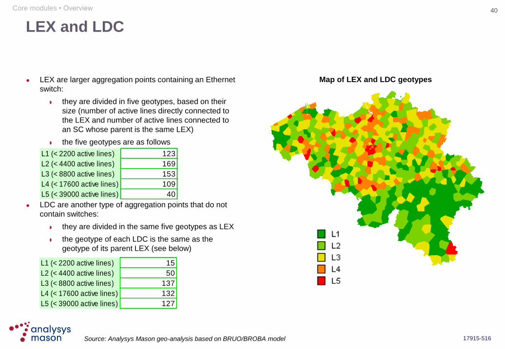
Map of LEX and LDC geotypes
LEX and LDC
LEX are larger aggregation points containing an Ethernet
switch:
they are divided in five geotypes, based on their
size (number of active lines directly connected to
the LEX and number of active lines connected to
an SC whose parent is the same LEX)
the five geotypes are as follows
LDC are another type of aggregation points that do not
contain switches:
they are divided in the same five geotypes as LEX
the geotype of each LDC is the same as the
geotype of its parent LEX (see below)
L1 (< 2200 active lines)
L2 (< 4400 active lines)
L3 (< 8800 active lines)
L4 (< 17600 active lines)
L5 (< 39000 active lines)
123
169
153
109
40
15
50
137
132
127
L1 (< 2200 active lines)
L2 (< 4400 active lines)
L3 (< 8800 active lines)
L4 (< 17600 active lines)
L5 (< 39000 active lines)
Core modules • Overview
Source: Analysys Mason geo-analysis based on BRUO/BROBA model
41
17915-516
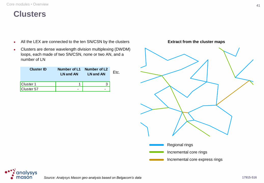
Extract from the cluster maps
Clusters
All the LEX are connected to the ten SN/CSN by the clusters
Clusters are dense wavelength division multiplexing (DWDM)
loops, each made of two SN/CSN, none or two AN, and a
number of LN
Source: Analysys Mason geo-analysis based on Belgacom’s data
Cluster ID
Cluster 1
Cluster 57
Number of L1
LN and AN
Number of L2
LN and AN
1 3
- -
Etc.
Regional rings
Incremental core rings
Incremental core express rings
Core modules • Overview
42
17915-516
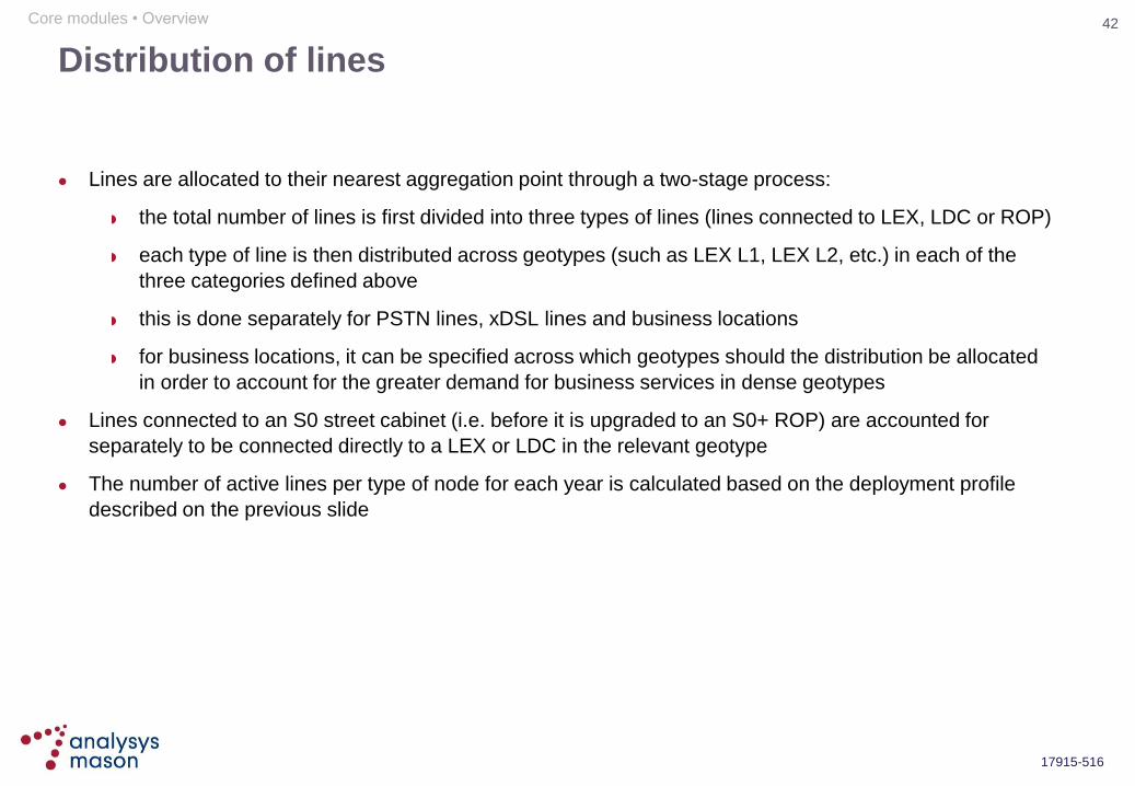
Distribution of lines
Lines are allocated to their nearest aggregation point through a two-stage process:
the total number of lines is first divided into three types of lines (lines connected to LEX, LDC or ROP)
each type of line is then distributed across geotypes (such as LEX L1, LEX L2, etc.) in each of the
three categories defined above
this is done separately for PSTN lines, xDSL lines and business locations
for business locations, it can be specified across which geotypes should the distribution be allocated
in order to account for the greater demand for business services in dense geotypes
Lines connected to an S0 street cabinet (i.e. before it is upgraded to an S0+ ROP) are accounted for
separately to be connected directly to a LEX or LDC in the relevant geotype
The number of active lines per type of node for each year is calculated based on the deployment profile
described on the previous slide
Core modules • Overview
43
17915-516
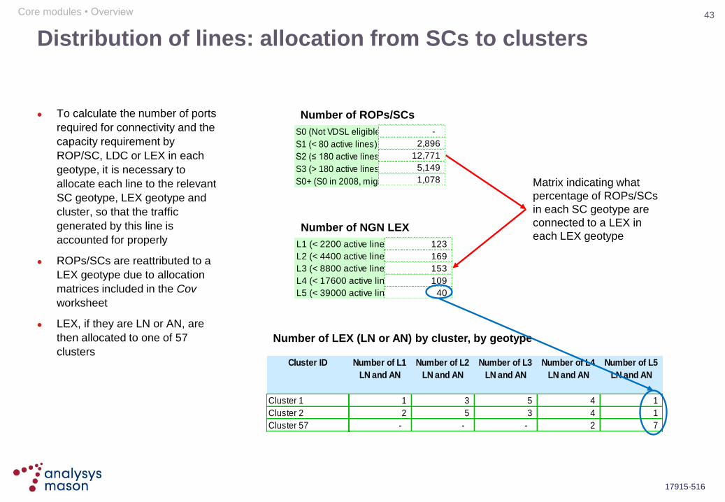
Distribution of lines: allocation from SCs to clusters
To calculate the number of ports
required for connectivity and the
capacity requirement by
ROP/SC, LDC or LEX in each
geotype, it is necessary to
allocate each line to the relevant
SC geotype, LEX geotype and
cluster, so that the traffic
generated by this line is
accounted for properly
ROPs/SCs are reattributed to a
LEX geotype due to allocation
matrices included in the Cov
worksheet
LEX, if they are LN or AN, are
then allocated to one of 57
clusters
Number of LEX (LN or AN) by cluster, by geotype
Cluster ID
Cluster 1
Cluster 2
Cluster 57
Number of L1
LN and AN
Number of L2
LN and AN
Number of L3
LN and AN
Number of L4
LN and AN
Number of L5
LN and AN
1 3 5 4 1
2 5 3 4 1
- - - 2 7
Number of NGN LEX
L1 (< 2200 active lines)
L2 (< 4400 active lines)
L3 (< 8800 active lines)
L4 (< 17600 active lines)
L5 (< 39000 active lines)
123
169
153
109
40
S0 (Not VDSL eligible yet in 2008)
S1 (< 80 active lines)
S2 (≤ 180 active lines)
S3 (> 180 active lines)
S0+ (S0 in 2008, migrated at a later date to VDSL)
-
2,896
12,771
5,149
1,078
Number of ROPs/SCs
Matrix indicating what
percentage of ROPs/SCs
in each SC geotype are
connected to a LEX in
each LEX geotype
Core modules • Overview

44
17915-516
Traffic allocation: from SCs to LEX
Share of SC in each geotype
connected to a LEX or to an LDC
Matrix allocating street cabinets to LEX geotypes (for LEX and
LDC combined, LEX only, LDC only)
Traffic by SC
geotype (except
linear IPTV)
Traffic by LEX
geotype (except
linear IPTV), for
SC
It means 88% of S1 SCs (ROPs) are connected to a
LEX, and 12% to a LDC
In this case (SC to LEX only), it means that 1% of S1 SCs (ROPs) are connected to a LEX in the
L1 geotype, 8% to a LEX in the L2 geotype, etc.
Traffic by LEX
geotype (except
linear IPTV), for
LEX and LDC
Total traffic by
LEX geotype
(except linear
IPTV)
Core modules • Overview
Colour key Input Calculations Output
LEX LDC
S0 (Not VDSL eligible yet in 2008) 89.0% 11.0%
S1 (< 80 active lines) 88.0% 12.0%
S2 (≤ 180 active lines) 92.0% 8.0%
S3 (> 180 active lines) 95.0% 5.0%
S0+ (S0 in 2008, migrated at a later date to VDSL)89.0% 11.0%
L1 (< 2200 active lines)L2 (< 4400 active lines)L3 (< 8800 active lines)L4 (< 17600 active lines)L5 (< 39000 active lines)
S0 (Not VDSL eligible yet in 2008) 10.0% 30.0% 31.0% 19.0% 10.0%
S1 (< 80 active lines) 1.0% 8.0% 35.0% 40.0% 16.0%
S2 (≤ 180 active lines) 3.0% 12.0% 24.0% 38.0% 23.0%
S3 (> 180 active lines) 4.0% 11.0% 19.0% 34.0% 32.0%
S0+ (S0 in 2008, migrated at a later date to VDSL)10.0% 30.0% 31.0% 19.0% 10.0%
45
17915-516
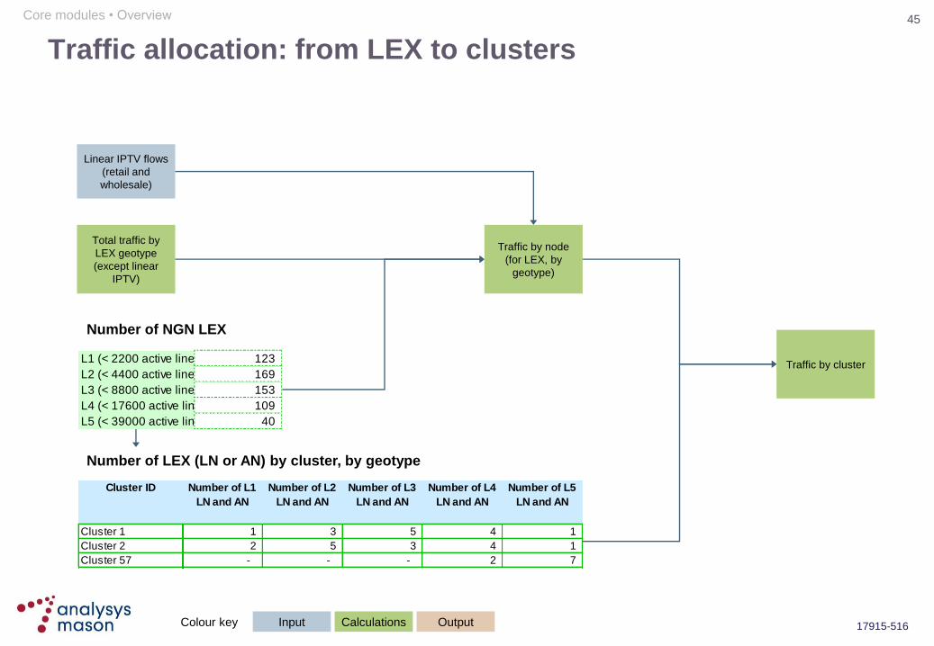
Traffic allocation: from LEX to clusters
Number of LEX (LN or AN) by cluster, by geotype
Number of NGN LEX
L1 (< 2200 active lines)
L2 (< 4400 active lines)
L3 (< 8800 active lines)
L4 (< 17600 active lines)
L5 (< 39000 active lines)
123
169
153
109
40
Cluster ID
Cluster 1
Cluster 2
Cluster 57
Number of L1
LN and AN
Number of L2
LN and AN
Number of L3
LN and AN
Number of L4
LN and AN
Number of L5
LN and AN
1 3 5 4 1
2 5 3 4 1
- - - 2 7
Traffic by node
(for LEX, by
geotype)
Traffic by cluster
Total traffic by
LEX geotype
(except linear
IPTV)
Linear IPTV flows
(retail and
wholesale)
Core modules • Overview
Colour key Input Calculations Output

46
17915-516
Network equipment deployment
A timeframe has been defined for the deployment of network equipment, starting with the deployment of Ethernet switches
It then follows a similar pattern for data and voice equipment, with equipment deployed as follows:
All LEX and LDC (and the IP-DSLAM they contain) are entirely deployed in 2005 (for all geotypes)
ROPs (and the SB-REMs they contain) are deployed from 2005, and S1, S2 and S3 are fully deployed by 2008, to match at
this date the number of ROPs deployed in the BRUO/BROBA model. S0+ are deployed from 2009
AGW in LEX and LDC are deployed from 2009 for all geotypes. They are all deployed by 2011 so the model can calculate a
regulated tariff based on the relevant amount of voice traffic from this year onwards
The deployment of AGW in ROP is defined as a period to reach the situation where all ROPs deployed in a given year
contain an AGW. It starts in 2009 and ends in 2011 (i.e. from 2011 all ROPs deployed contain an AGW), for the same reason
it ends in 2011 for AGW in LEX and LDC
All these values flow into the „Cov‟ worksheet to define the number of LEX, LDC and ROPs (with AGW)
Deployment order Data equipment Voice equipment
1 IP-DSLAM LEX-AGW
2 SB-REM aggregators AGG-AGW
3 SB-REM DSLAMs ROP-AGW
Core modules • Overview
47
17915-516
Model overview
Market module
NGN data connectivity
Overview
Core modules
Access modules
Service costing modules
Ancillary/common/overhead modules
Demand conversion
NGN voice connectivity
Ethernet/IP core Service platforms
Introduction
Glossary
48
17915-516
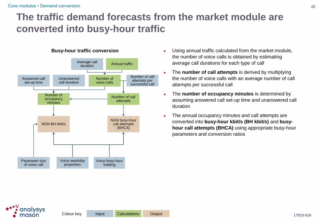
The traffic demand forecasts from the market module are
converted into busy-hour traffic
Using annual traffic calculated from the market module,
the number of voice calls is obtained by estimating
average call durations for each type of call
The number of call attempts is derived by multiplying
the number of voice calls with an average number of call
attempts per successful call
The number of occupancy minutes is determined by
assuming answered call set-up time and unanswered call
duration
The annual occupancy minutes and call attempts are
converted into busy-hour kbit/s (BH kbit/s) and busy-
hour call attempts (BHCA) using appropriate busy-hour
parameters and conversion ratios
Number of voice calls
Number of call attempts
Number of call attempts per
successful call
Number of occupancy
minutes
Answered call set-up time
Unanswered call duration
Annual traffic Average call
duration
NGN busy-hour call attempts
(BHCA) NGN BH kbit/s
Voice weekday proportion
Voice busy-hour loading
Busy-hour traffic conversion
Core modules • Demand conversion
Parameter size of voice call
Colour key Input Calculations Output

49
17915-516
Busy-hour traffic is then re-organised into network
services traffic
On-net traffic is divided into two categories:
regional on-net calls, switched/routed at one core
node
national on-net calls, switched/routed at two core
nodes
localisation factors are used to take into account
the greater likelihood to call someone in the same
region
Outgoing traffic is similarly divided into two categories
The NGN interconnection SS7 and SIP network services
are modelled separately using a SS7 SIP migration
profile
No. call regions
Localisation factors
On-net: regional proportion
On-net: national proportion
Outgoing: regional
proportion
Outgoing: national
proportion
Localisation factors
NGN outgoing SS7 leg
NGN outgoing SIP leg
NGN regional outgoing
NGN national outgoing
NGN regional transit
NGN national transit
Network services traffic conversion
Core modules • Demand conversion
NGN regional transit
NGN national transit
NGN incoming SS7 leg
NGN incoming SIP leg
SS7 SIP migration
profile
Colour key Input Calculations Output

50
17915-516
Finally, a routeing matrix converts network services traffic
into network loading by asset groups
The routeing matrix specifies the load of each service on
each network asset group
A snapshot of part of the routeing matrix is shown below
Routeing matrix
Asset groups
Netw
ork
serv
ices
… Asset 2 Asset 1
…
service 2
service 1
Network services traffic demand
Loading on each asset group
Network loading conversion
Screenshot of routeing matrix
Core modules • Demand conversion
IP Distribution
transmission
IP Core
transmission
EthSw-SR SR-SR
2 -
2 1
- -
1 -
1 1
- -
- -
- -
- -
1 -
1 1
Network services Nodes routing
NGN Regional on-net calls AGW-EthSw-SR-EthSw-AGW
NGN National on-net calls AGW-EthSw-SR-SR-EthSw-AGW
spare spare
NGN Regional outgoing calls AGW-EthSw-SR…
NGN National outgoing calls AGW-EthSw-SR-SR…
spare spare
NGN Outgoing ss7 leg ...-SBC-<c>-TGW-other operators
NGN Outgoing SIP leg ...-SBC-PR-other operators
spare spare
NGN Regional incoming calls …SR-EthSw-AGW
NGN National incoming calls …SR-SR-EthSw-AGW

51
17915-516
Model overview
Market module
NGN data connectivity
Overview
Core modules
Access modules
Service costing modules
Ancillary/common/overhead modules
Demand conversion
NGN voice connectivity
Ethernet/IP core Service platforms
Introduction
Glossary
52
17915-516
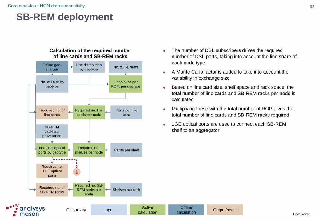
Calculation of the required number
of line cards and SB-REM racks
No. of ROP by
geotype
Lines/subs per
ROP, per geotype
No. xDSL subs Line distribution
by geotype
Ports per line
card
Required no. line
cards per node
Cards per shelf Required no.
shelves per node
Shelves per rack
Required no. SB-
REM racks per
node
Required no. of
SB-REM racks
Required no. of
line cards
Required no.
1GE optical
ports
Offline geo-
analysis
SB-REM deployment
SB-REM
backhaul
provisioned
No. 1GE optical
ports by geotype
1
Core modules • NGN data connectivity
The number of DSL subscribers drives the required
number of DSL ports, taking into account the line share of
each node type
A Monte Carlo factor is added to take into account the
variability in exchange size
Based on line card size, shelf space and rack space, the
total number of line cards and SB-REM racks per node is
calculated
Multiplying these with the total number of ROP gives the
total number of line cards and SB-REM racks required
1GE optical ports are used to connect each SB-REM
shelf to an aggregator
Colour key Input „Active‟
calculation Output/result
„Offline‟
calculation

53
17915-516
Calculation of the required number of SB-REM aggregators
No. of LEX by
geotype
1GE ports per
LEX, per geotype
No. 1GE optical
ports by SC
geotype
Allocation of
ROP from ROP
geotypes to LEX
geotypes
Ports per
aggregator
Required no.
aggregators per
LEX
Required no. of
aggregators
Offline geo-
analysis
SB-REM aggregators deployment
1
No. 1GE optical
ports by LEX
geotype
No. aggregators
by LEX geotype
2
Core modules • NGN data connectivity
The number of aggregators-facing ports on SB-REM by
SC geotype is reallocated by LEX geotypes using the
appropriate allocation matrix to determine the number of
SB-REM facing ports by LEX geotype
This number is then divided by the number of LEX by
geotype to obtain an average number of ports by LEX,
by geotype
Based on the number of ports by aggregator, a number of
aggregators per LEX, by geotype, is calculated
Multiplying these with the total number of LEX, by
geotype, gives the total number of aggregators required
Colour key Input „Active‟
calculation Output/result
„Offline‟
calculation
54
17915-516
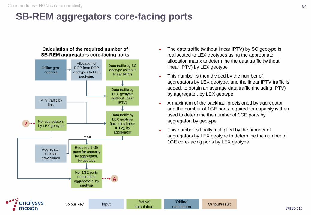
Calculation of the required number of
SB-REM aggregators core-facing ports
Data traffic by
LEX geotype
(including linear
IPTV), by
aggregator
Data traffic by SC
geotype (without
linear IPTV)
Allocation of
ROP from ROP
geotypes to LEX
geotypes
Aggregator
backhaul
provisioned
Required 1 GE
ports for capacity
by aggregator,
by geotype
Offline geo-
analysis
SB-REM aggregators core-facing ports
Data traffic by
LEX geotype
(without linear
IPTV)
No. 1GE ports
required for
aggregators, by
geotype
2
MAX
A
IPTV traffic by
link
No. aggregators
by LEX geotype
Core modules • NGN data connectivity
The data traffic (without linear IPTV) by SC geotype is
reallocated to LEX geotypes using the appropriate
allocation matrix to determine the data traffic (without
linear IPTV) by LEX geotype
This number is then divided by the number of
aggregators by LEX geotype, and the linear IPTV traffic is
added, to obtain an average data traffic (including IPTV)
by aggregator, by LEX geotype
A maximum of the backhaul provisioned by aggregator
and the number of 1GE ports required for capacity is then
used to determine the number of 1GE ports by
aggregator, by geotype
This number is finally multiplied by the number of
aggregators by LEX geotype to determine the number of
1GE core-facing ports by LEX geotype
Colour key Input „Active‟
calculation Output/result
„Offline‟
calculation

55
17915-516
Calculation of the required number
of line cards and IPDSLAM racks
No. of LEX by
geotype
Lines/subs per
LEX, per geotype
No. xDSL subs Line distribution
by LEX geotype
Ports per line
card
Required no. line
cards per node
Cards per shelf Required no.
shelves per node
Shelves per rack
Required no. SB-
REM racks per
node
Required no. of
IP-DSLAM racks,
by geotype
Required no. of
line cards
Offline geo-
analysis
IP-DSLAM deployment
Allocation of S0
from ROP
geotypes to LEX
geotypes
Line distribution
by ROP geotype
Required no. of
IP-DSLAM racks 3
Core modules • NGN data connectivity
The number of xDSL subscribers connected to an S0
(SC not yet migrated to a ROP), which is itself connected to
a LEX, is reallocated to LEX geotypes, added to the
subscribers directly connected to the LEX, and the total is
divided by the number of LEX to obtain the number of
lines/subscribers by LEX, by geotype
The number of ports per line card, cards per shelf and
shelves per rack, and their utilisation factor are then used to
calculate the number of line cards, shelves and racks per
LEX. A Monte Carlo input is used for line cards and shelves
to take into account the variability in exchange size
Line cards and racks per LEX are then multiplied by the
number of LEX, by geotype, to obtain the total number of
line cards and racks required for LEX
The exact same calculations are run for xDSL subscribers
directly connected to an LDC or an S0 connected to an LDC
The required number of line cards and racks for LEX and
LDC are finally added together to obtain the total number of
line cards and IP-DSLAM racks required
Colour key Input „Active‟
calculation Output/result
„Offline‟
calculation
56
17915-516
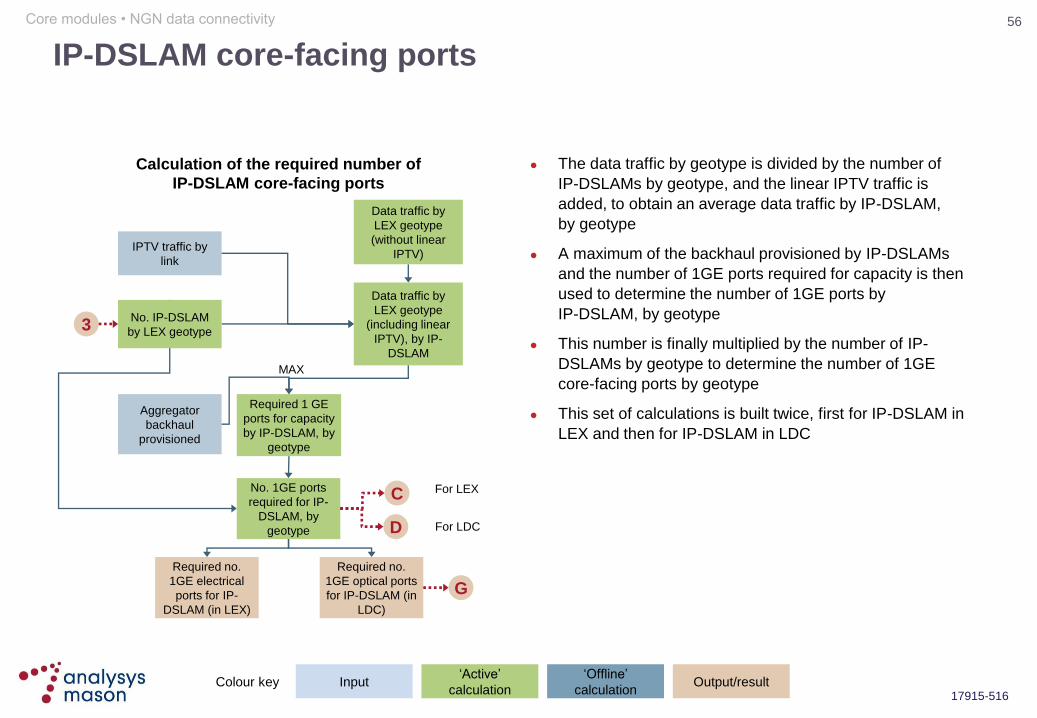
Calculation of the required number of
IP-DSLAM core-facing ports
Data traffic by
LEX geotype
(including linear
IPTV), by IP-
DSLAM
Aggregator
backhaul
provisioned
Required 1 GE
ports for capacity
by IP-DSLAM, by
geotype
IP-DSLAM core-facing ports
Data traffic by
LEX geotype
(without linear
IPTV)
No. 1GE ports
required for IP-
DSLAM, by
geotype
3
MAX
C
IPTV traffic by
link
No. IP-DSLAM
by LEX geotype
D
For LEX
For LDC
Required no.
1GE electrical
ports for IP-
DSLAM (in LEX)
Required no.
1GE optical ports
for IP-DSLAM (in
LDC)
G
Core modules • NGN data connectivity
The data traffic by geotype is divided by the number of
IP-DSLAMs by geotype, and the linear IPTV traffic is
added, to obtain an average data traffic by IP-DSLAM,
by geotype
A maximum of the backhaul provisioned by IP-DSLAMs
and the number of 1GE ports required for capacity is then
used to determine the number of 1GE ports by
IP-DSLAM, by geotype
This number is finally multiplied by the number of IP-
DSLAMs by geotype to determine the number of 1GE
core-facing ports by geotype
This set of calculations is built twice, first for IP-DSLAM in
LEX and then for IP-DSLAM in LDC
Colour key Input „Active‟
calculation Output/result
„Offline‟
calculation
57
17915-516
Model overview
Market module
NGN data connectivity
Overview
Core modules
Access modules
Service costing modules
Ancillary/common/overhead modules
Demand conversion
NGN voice connectivity
Ethernet/IP core Service platforms
Introduction
Glossary
58
17915-516
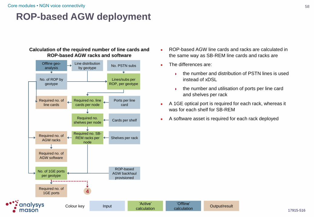
Calculation of the required number of line cards and
ROP-based AGW racks and software
ROP-based AGW deployment
No. of ROP by
geotype
Lines/subs per
ROP, per geotype
No. PSTN subs Line distribution
by geotype
Ports per line
card
Required no. line
cards per node
Cards per shelf Required no.
shelves per node
Shelves per rack
Required no. SB-
REM racks per
node
Required no. of
AGW racks
Required no. of
line cards
Offline geo-
analysis
Required no. of
AGW software
ROP-based
AGW backhaul
provisioned
No. of 1GE ports
per geotype
Required no. of
1GE ports 4
Core modules • NGN voice connectivity
ROP-based AGW line cards and racks are calculated in
the same way as SB-REM line cards and racks are
The differences are:
the number and distribution of PSTN lines is used
instead of xDSL
the number and utilisation of ports per line card
and shelves per rack
A 1GE optical port is required for each rack, whereas it
was for each shelf for SB-REM
A software asset is required for each rack deployed
Colour key Input „Active‟
calculation Output/result
„Offline‟
calculation

59
17915-516
Calculation of the required number of AGW aggregators
No. of LEX by
geotype
1GE ports per
LEX, per geotype
No. 1GE optical
ports by SC
geotype
Allocation of ROP
from ROP
geotypes to LEX
geotypes
Ports per AGW
aggregator
Required no.
AGW aggregators
per LEX
Required no. of
AGW
aggregators
Offline geo-
analysis
Deployment of AGW aggregators
4
No. 1GE optical
ports by LEX
geotype
No. AGW
aggregators by
LEX geotype
5
Core modules • NGN voice connectivity
The deployment of AGW aggregators is determined in
the same way as the deployment of SB-REM aggregators
The number of AGW aggregators-facing ports on ROP-
AGW by SC geotype is reallocated by LEX geotype using
the SC-to-LEX allocation matrix described previously to
determine the number of ROP-AGW-facing ports by LEX
geotype
This number is then divided by the number of LEX by
geotype to obtain an average number of ports by LEX,
by geotype
Based on the number of ports by AGW aggregators, a
number of aggregators per LEX is calculated
Multiplying these by the total number of LEX, by geotype,
gives the total number of AGW aggregators required
Colour key Input „Active‟
calculation Output/result
„Offline‟
calculation

60
17915-516
Calculation of the required number of
AGW aggregators core-facing ports
Voice traffic by
LEX geotype, by
AGW aggregator
Voice traffic by
SC geotype
Allocation of ROP
from ROP geotypes
to LEX geotypes
Aggregator
backhaul
provisioned
Required 1 GE
ports for capacity by
AGW aggregator ,
by geotype
Offline geo-
analysis
AGG aggregators core-facing ports
Voice traffic by
LEX geotype
No. 1GE ports
required for AGW
aggregator, by
geotype
5
MAX
B
No. AGW
aggregators by
LEX geotype
Core modules • NGN voice connectivity
The number of AGW aggregators core-facing ports is
calculated in the same way as the number of SB-REM
aggregators core-facing ports, but using voice traffic
instead of data traffic (and therefore ignoring linear IPTV)
The voice traffic by SC geotype is reallocated by LEX
geotype using the appropriate allocation matrix to
determine the voice traffic by LEX geotype
This number is then divided by the number of AGW
aggregators by LEX geotype to obtain an average voice
traffic by AGW aggregator, by LEX geotype
A maximum of the backhaul provisioned by AGW
aggregator and the number of 1GE ports required for
capacity is then used to determine the number of 1GE
ports by AGW aggregator, by geotype
This number is finally multiplied by the number of AGW
aggregators by LEX geotype to determine the number of
1GE core-facing ports by LEX geotype
Colour key Input „Active‟
calculation Output/result
„Offline‟
calculation
61
17915-516
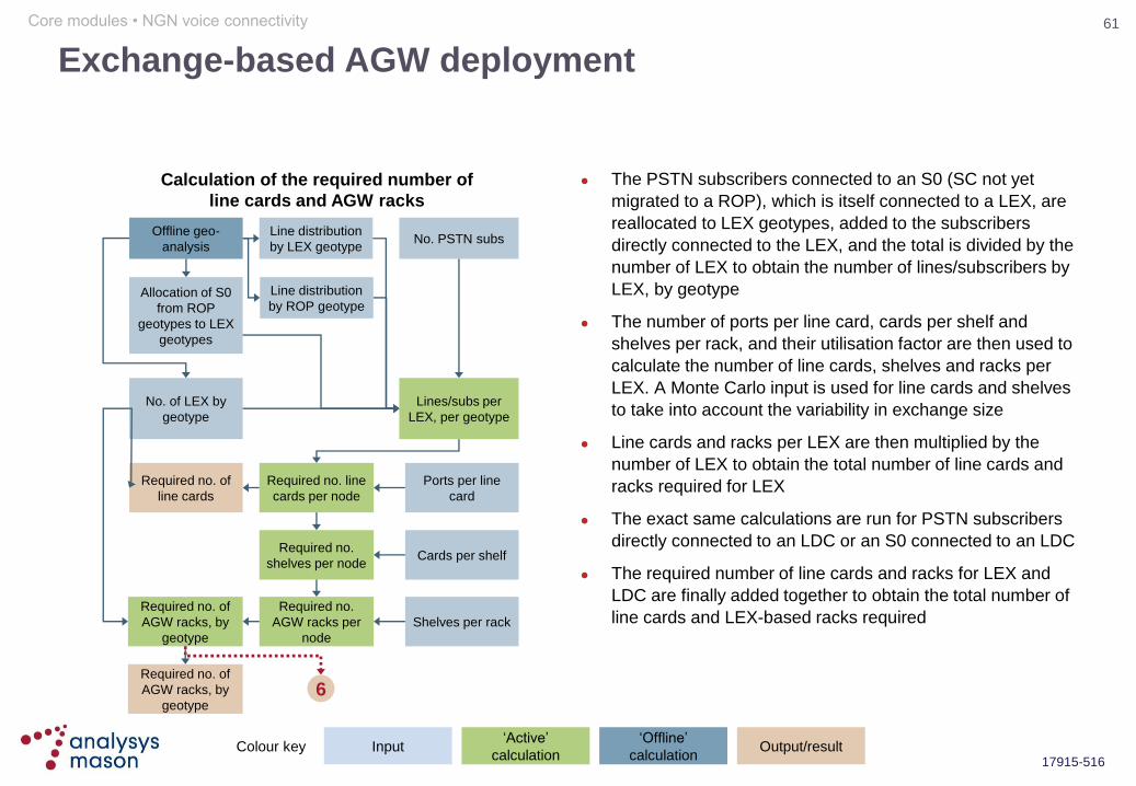
Calculation of the required number of
line cards and AGW racks
No. of LEX by
geotype
Lines/subs per
LEX, per geotype
No. PSTN subs Line distribution
by LEX geotype
Ports per line
card
Required no. line
cards per node
Cards per shelf Required no.
shelves per node
Shelves per rack
Required no.
AGW racks per
node
Required no. of
AGW racks, by
geotype
Required no. of
line cards
Offline geo-
analysis
Exchange-based AGW deployment
Allocation of S0
from ROP
geotypes to LEX
geotypes
Line distribution
by ROP geotype
Required no. of
AGW racks, by
geotype 6
Core modules • NGN voice connectivity
The PSTN subscribers connected to an S0 (SC not yet
migrated to a ROP), which is itself connected to a LEX, are
reallocated to LEX geotypes, added to the subscribers
directly connected to the LEX, and the total is divided by the
number of LEX to obtain the number of lines/subscribers by
LEX, by geotype
The number of ports per line card, cards per shelf and
shelves per rack, and their utilisation factor are then used to
calculate the number of line cards, shelves and racks per
LEX. A Monte Carlo input is used for line cards and shelves
to take into account the variability in exchange size
Line cards and racks per LEX are then multiplied by the
number of LEX to obtain the total number of line cards and
racks required for LEX
The exact same calculations are run for PSTN subscribers
directly connected to an LDC or an S0 connected to an LDC
The required number of line cards and racks for LEX and
LDC are finally added together to obtain the total number of
line cards and LEX-based racks required
Colour key Input „Active‟
calculation Output/result
„Offline‟
calculation
62
17915-516
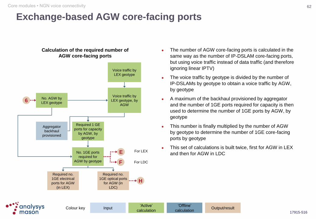
Calculation of the required number of
AGW core-facing ports
Voice traffic by
LEX geotype, by
AGW
Aggregator
backhaul
provisioned
Required 1 GE
ports for capacity
by AGW, by
geotype
Exchange-based AGW core-facing ports
Voice traffic by
LEX geotype
No. 1GE ports
required for
AGW by geotype
6
For LDC
E
No. AGW by
LEX geotype
F
Required no.
1GE electrical
ports for AGW
(in LEX)
Required no.
1GE optical ports
for AGW (in
LDC)
For LEX
H
Core modules • NGN voice connectivity
The number of AGW core-facing ports is calculated in the
same way as the number of IP-DSLAM core-facing ports,
but using voice traffic instead of data traffic (and therefore
ignoring linear IPTV)
The voice traffic by geotype is divided by the number of
IP-DSLAMs by geotype to obtain a voice traffic by AGW,
by geotype
A maximum of the backhaul provisioned by aggregator
and the number of 1GE ports required for capacity is then
used to determine the number of 1GE ports by AGW, by
geotype
This number is finally multiplied by the number of AGW
by geotype to determine the number of 1GE core-facing
ports by geotype
This set of calculations is built twice, first for AGW in LEX
and then for AGW in LDC
Colour key Input „Active‟
calculation Output/result
„Offline‟
calculation
63
17915-516
Model overview
Market module
NGN data connectivity
Overview
Core modules
Access modules
Service costing modules
Ancillary/common/overhead modules
Demand conversion
NGN voice connectivity
Ethernet/IP core Service platforms
Introduction
Glossary
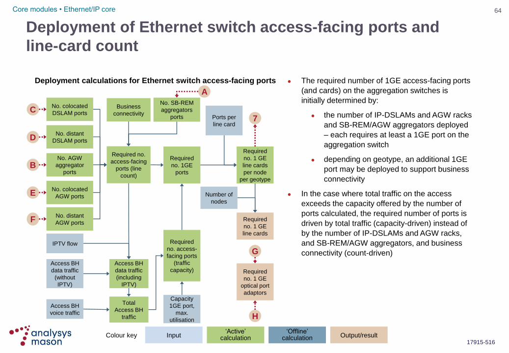
64
17915-516
No. colocated
DSLAM ports
Access BH
data traffic
(without
IPTV)
Access BH
data traffic
(including
IPTV)
Capacity
1GE port,
max.
utilisation
Required
no. access-
facing ports
(traffic
capacity)
Required no.
access-facing
ports (line
count)
Required
no. 1GE
ports
No. SB-REM
aggregators
ports
The required number of 1GE access-facing ports
(and cards) on the aggregation switches is
initially determined by:
the number of IP-DSLAMs and AGW racks
and SB-REM/AGW aggregators deployed
– each requires at least a 1GE port on the
aggregation switch
depending on geotype, an additional 1GE
port may be deployed to support business
connectivity
In the case where total traffic on the access
exceeds the capacity offered by the number of
ports calculated, the required number of ports is
driven by total traffic (capacity-driven) instead of
by the number of IP-DSLAMs and AGW racks,
and SB-REM/AGW aggregators, and business
connectivity (count-driven)
Business
connectivity
Deployment of Ethernet switch access-facing ports and
line-card count
7
No. distant
DSLAM ports
No. colocated
AGW ports
No. AGW
aggregator
ports
No. distant
AGW ports
Deployment calculations for Ethernet switch access-facing ports
IPTV flow
Access BH
voice traffic
Total
Access BH
traffic
Required
no. 1 GE
line cards
per node
per geotype
Required
no. 1 GE
optical port
adaptors
Ports per
line card
Required
no. 1 GE
line cards
Number of
nodes
C
F
E
D
B
A
G
H
Core modules • Ethernet/IP core
Colour key Input „Active‟
calculation Output/result „Offline‟
calculation
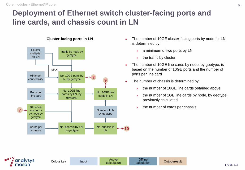
65
17915-516
Deployment of Ethernet switch cluster-facing ports and
line cards, and chassis count in LN
The number of 10GE cluster-facing ports by node for LN
is determined by:
a minimum of two ports by LN
the traffic by cluster
The number of 10GE line cards by node, by geotype, is
based on the number of 10GE ports and the number of
ports per line card
The number of chassis is determined by:
the number of 10GE line cards obtained above
the number of 1GE line cards by node, by geotype,
previously calculated
the number of cards per chassis
Cluster-facing ports in LN
Traffic by node by
geotype
No. 10GE ports by
LN, by geotype,
Cards per
chassis
Ports per
line card
No. 10GE line
cards by LN, by
geotype,
7 No. 1 GE
line cards
by node by
geotype
No. chassis by LN,
by geotype
Number of LN
by geotype
No. 10GE line
cards in LN
No. chassis in
LN
9
10
8
Core modules • Ethernet/IP core
MAX
Minimum
connectivity
Cluster
multiplier
for LN
Colour key Input „Active‟
calculation Output/result „Offline‟
calculation

66
17915-516
Deployment of Ethernet switch cluster-facing ports and
line-card/chassis count in AN
The number of 10GE cluster-facing ports by node for AN
is determined based on the number of lambdas for
clusters with AN on each core ring
It then follows the same type of calculations used to
determine the number of line cards and chassis for LN,
but does this by core ring rather than by geotype
Cluster-facing ports in AN
Core modules • Ethernet/IP core
Offline geo-
analysis
Number of AN
by core ring
Cards per
chassis
7 No. 1 GE
line cards
by node by
geotype
No. chassis by
AN, by geotype,
by core ring
Number of AN by
core ring
No. 10GE line
cards in AN
No. chassis in AN
No. lambdas by
cluster 11
No. lambdas for
clusters with AN
by core ring
Clusters with AN
by core ring
No. lambdas by
AN, by core ring
No. 10GE ports by
AN, by core ring
Cluster
multiplier for
AN
Ports per
line card
No. 10GE line
cards by AN, by
core ring
14
15
12
13
Capacity by
lambda
Number of LN
and AN of each
geotype by
cluster
Traffic by node by
geotype
Traffic by cluster
Colour key Input „Active‟
calculation Output/result „Offline‟
calculation
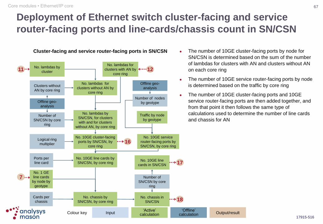
67
17915-516
Deployment of Ethernet switch cluster-facing and service
router-facing ports and line-cards/chassis count in SN/CSN
The number of 10GE cluster-facing ports by node for
SN/CSN is determined based on the sum of the number
of lambdas for clusters with AN and clusters without AN
on each core ring
The number of 10GE service router-facing ports by node
is determined based on the traffic by core ring
The number of 10GE cluster-facing ports and 10GE
service router-facing ports are then added together, and
from that point it then follows the same type of
calculations used to determine the number of line cards
and chassis for AN
Cluster-facing and service router-facing ports in SN/CSN
Offline geo-
analysis
Number of
SN/CSN by core
ring
Cards per
chassis
7 No. 1 GE
line cards
by node by
geotype
No. chassis by
SN/CSN, by core ring
Number of
SN/CSN by core
ring
No. 10GE line
cards in SN/CSN
No. chassis in
SN/CSN
No. lambdas by
cluster 11
No. lambdas for
clusters without AN by
core ring
Clusters without
AN by core ring
No. lambdas by
SN/CSN, for clusters
with and for clusters
without AN, by core ring
No. 10GE cluster-facing
ports by SN/CSN, by
core ring
Logical ring
multiplier
Ports per
line card
No. 10GE line cards by
SN/CSN, by core ring 17
18
No. lambdas for
clusters with AN by
core ring 12
Traffic by node
by geotype
Offline geo-
analysis
Number of nodes
by geotype
No. 10GE service
router-facing ports by
SN/CSN, by core ring 16
Core modules • Ethernet/IP core
Colour key Input „Active‟
calculation Output/result „Offline‟
calculation

68
17915-516
Ethernet switch total line cards and chassis count
Finally, the 10GE line cards and chassis counts of LN,
AN and SN/CSN are added together to give the total
number of 10GE line cards and chassis in Ethernet
switches
Ethernet switch line cards and chassis count
No. 10GE line
cards in LN
No. 10GE line
cards in AN
9
14
No. 10GE line
cards in SN/CSN
No. chassis in LN
17
10
No. chassis in AN
No. chassis in
SN/CSN
15
18
Total No. 10GE
line card
Total No. chassis
Core modules • Ethernet/IP core
Colour key Input „Active‟
calculation Output/result „Offline‟
calculation
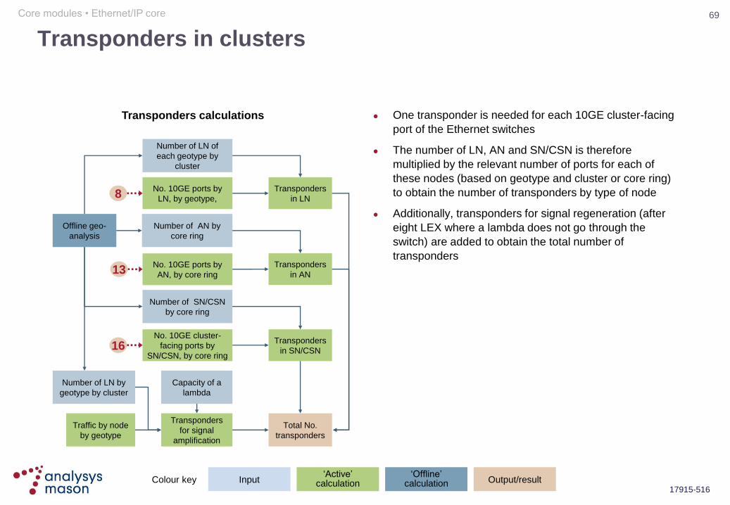
69
17915-516
Transponders in clusters
One transponder is needed for each 10GE cluster-facing
port of the Ethernet switches
The number of LN, AN and SN/CSN is therefore
multiplied by the relevant number of ports for each of
these nodes (based on geotype and cluster or core ring)
to obtain the number of transponders by type of node
Additionally, transponders for signal regeneration (after
eight LEX where a lambda does not go through the
switch) are added to obtain the total number of
transponders
Transponders calculations
No. 10GE ports by
LN, by geotype,
No. 10GE ports by
AN, by core ring
8
13
No. 10GE cluster-
facing ports by
SN/CSN, by core ring 16
Offline geo-
analysis
Number of LN of
each geotype by
cluster
Number of AN by
core ring
Number of SN/CSN
by core ring
Transponders
in LN
Transponders
in SN/CSN
Transponders
in AN
Total No.
transponders
Traffic by node
by geotype
Number of LN by
geotype by cluster
Capacity of a
lambda
Transponders
for signal
amplification
Core modules • Ethernet/IP core
Colour key Input „Active‟
calculation Output/result „Offline‟
calculation

70
17915-516
ADM in clusters
The number of ADM required is calculated using a similar
method as for transponders, but also taking into account
the number of transponders that can fit on an ADM
Transponder calculations
No. 10GE ports by
LN, by geotype, by
cluster
No. 10GE ports by
AN, by core ring
8
13
No. 10GE cluster-
facing ports by
SN/CSN, by core ring 16
Offline geo-
analysis
Number of of each
geotype by cluster
Number of AN by
core ring
Number of SN/CSN
by core ring
ADM in LN
ADM in
SN/CSN
ADM in AN
Total No. ADM
Transponders
per ADM
Transponders
per ADM
Transponders
per ADM
Core modules • Ethernet/IP core
Colour key Input „Active‟
calculation Output/result „Offline‟
calculation
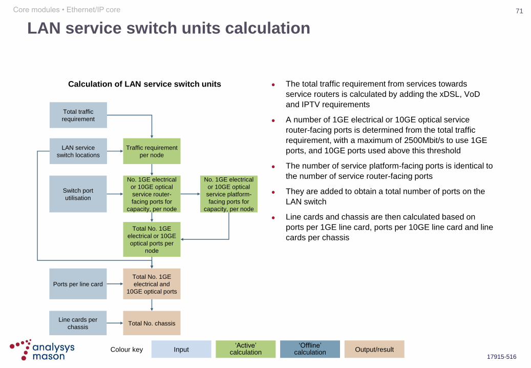
71
17915-516
LAN service switch units calculation
The total traffic requirement from services towards
service routers is calculated by adding the xDSL, VoD
and IPTV requirements
A number of 1GE electrical or 10GE optical service
router-facing ports is determined from the total traffic
requirement, with a maximum of 2500Mbit/s to use 1GE
ports, and 10GE ports used above this threshold
The number of service platform-facing ports is identical to
the number of service router-facing ports
They are added to obtain a total number of ports on the
LAN switch
Line cards and chassis are then calculated based on
ports per 1GE line card, ports per 10GE line card and line
cards per chassis
Calculation of LAN service switch units
Total traffic
requirement
Total No. 1GE
electrical and
10GE optical ports
Switch port
utilisation
LAN service
switch locations
Traffic requirement
per node
No. 1GE electrical
or 10GE optical
service router-
facing ports for
capacity, per node
No. 1GE electrical
or 10GE optical
service platform-
facing ports for
capacity, per node
Total No. 1GE
electrical or 10GE
optical ports per
node
Ports per line card
Line cards per
chassis Total No. chassis
Core modules • Ethernet/IP core
Colour key Input „Active‟
calculation Output/result „Offline‟
calculation
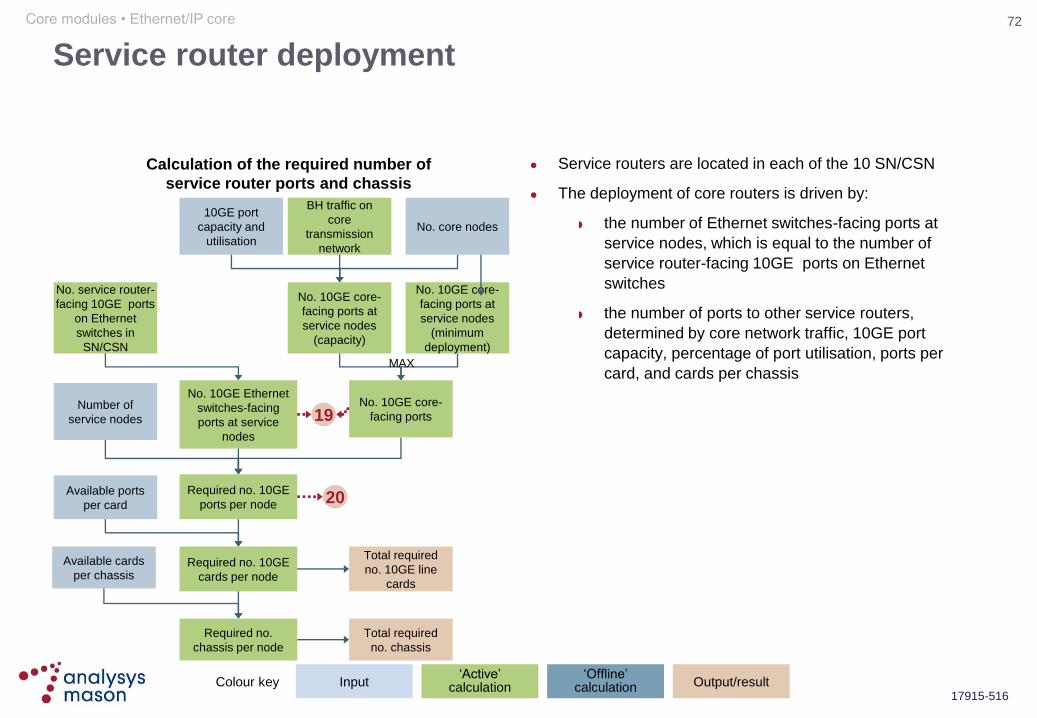
72
17915-516
Service router deployment
Service routers are located in each of the 10 SN/CSN
The deployment of core routers is driven by:
the number of Ethernet switches-facing ports at
service nodes, which is equal to the number of
service router-facing 10GE ports on Ethernet
switches
the number of ports to other service routers,
determined by core network traffic, 10GE port
capacity, percentage of port utilisation, ports per
card, and cards per chassis
Calculation of the required number of
service router ports and chassis
Core modules • Ethernet/IP core
No. service router-
facing 10GE ports
on Ethernet
switches in
SN/CSN
No. 10GE Ethernet
switches-facing
ports at service
nodes
BH traffic on
core
transmission
network
No. 10GE core-
facing ports at
service nodes
(capacity)
Required no. 10GE
cards per node
Available ports
per card
Available cards
per chassis
No. core nodes
No. 10GE core-
facing ports at
service nodes
(minimum
deployment)
10GE port
capacity and
utilisation
No. 10GE core-
facing ports
MAX
Required no.
chassis per node
Total required
no. chassis
Total required
no. 10GE line
cards
Required no. 10GE
ports per node
Number of
service nodes 19
20
Colour key Input „Active‟
calculation Output/result „Offline‟
calculation

73
17915-516
Transponders and ADM for service routers
One transponder is required for every 10GE port
One ADM is required for every 40 transponders in each
service node
Transponders and ADM calculations
No. 10GE ports 19
Total No. ADM Transponders per
ADM
Total No.
transponders
Number of service
nodes
Core modules • Ethernet/IP core
No. 10GE ports
per node 20
Colour key Input „Active‟
calculation Output/result „Offline‟
calculation

74
17915-516
Model overview
Market module
NGN data connectivity
Overview
Core modules
Access modules
Service costing modules
Ancillary/common/overhead modules
Demand conversion
NGN voice connectivity
Ethernet/IP core Service platforms
Introduction
Glossary
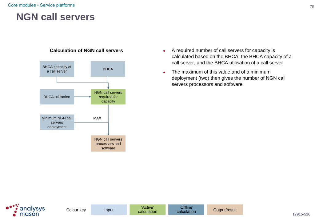
75
17915-516
NGN call servers
A required number of call servers for capacity is
calculated based on the BHCA, the BHCA capacity of a
call server, and the BHCA utilisation of a call server
The maximum of this value and of a minimum
deployment (two) then gives the number of NGN call
servers processors and software
Calculation of NGN call servers
BHCA capacity of
a call server
NGN call servers
required for
capacity
BHCA
NGN call servers
processors and
software
BHCA utilisation
Minimum NGN call
servers
deployment
MAX
Core modules • Service platforms
Colour key Input „Active‟
calculation Output/result „Offline‟
calculation

76
17915-516
Deployment of trunk gateways
A minimum of one gateway is required for each NGN
SS7 PoI node
Additional gateways are installed to accommodate
interconnection traffic requirements. This is driven by:
NGN SS7 interconnection traffic
core E1 capacity and utilisation
E1 ports per gateway
The number of 1GE SBC-facing ports can be obtained by
assuming an average number of equipment per gateway
Trunk gateways
Core modules • Service platforms
NGN SS7 voice
interconnection
traffic (Mbit/s)
NGN SS7 voice
interconnection
traffic (BHE)
No. MGW-
national
interconnection
circuit groups
No. circuit
groups
BHE per circuit
group
No. E1s per
circuit group Erlang table
Core E1 capacity
Core E1
utilisation
No. E1s
E1 ports per
gateway
No. gateway
required for
capacity
Minimum
gateway
deployment
No. NGN SS7
PoI nodes
Gateways
required
MAX
21
22
1GE SBC-facing
ports per
gateway
Interco 1GE
SBC-facing ports
Colour key Input „Active‟
calculation Output/result „Offline‟
calculation
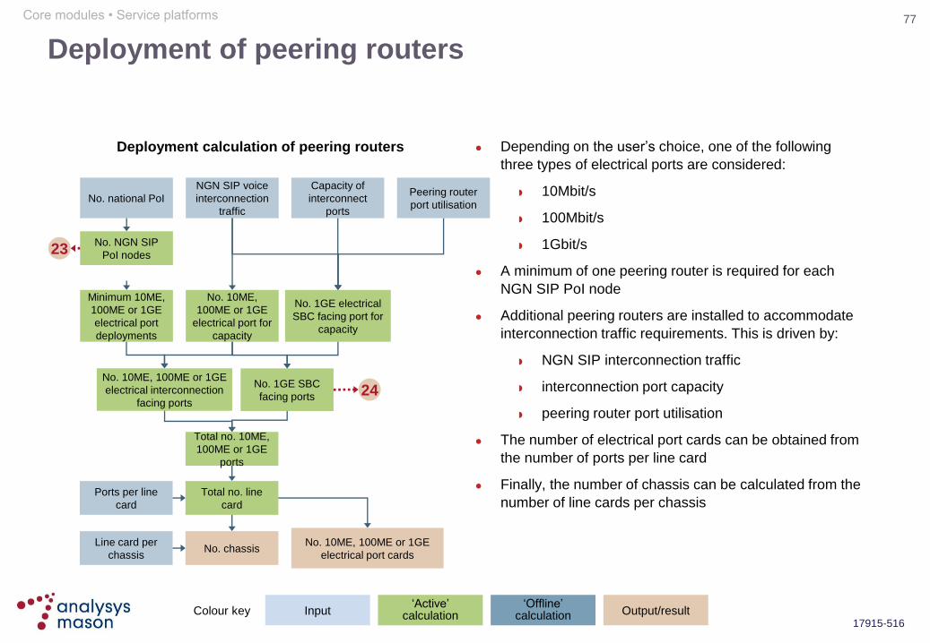
77
17915-516
Deployment of peering routers
Depending on the user‟s choice, one of the following
three types of electrical ports are considered:
10Mbit/s
100Mbit/s
1Gbit/s
A minimum of one peering router is required for each
NGN SIP PoI node
Additional peering routers are installed to accommodate
interconnection traffic requirements. This is driven by:
NGN SIP interconnection traffic
interconnection port capacity
peering router port utilisation
The number of electrical port cards can be obtained from
the number of ports per line card
Finally, the number of chassis can be calculated from the
number of line cards per chassis
Deployment calculation of peering routers
NGN SIP voice
interconnection
traffic
Capacity of
interconnect
ports
No. NGN SIP
PoI nodes
No. national PoI
Minimum 10ME,
100ME or 1GE
electrical port
deployments
No. 10ME, 100ME or 1GE
electrical interconnection
facing ports
No. 10ME,
100ME or 1GE
electrical port for
capacity
Peering router
port utilisation
No. 1GE electrical
SBC facing port for
capacity
No. 1GE SBC
facing ports
Total no. 10ME,
100ME or 1GE
ports
Ports per line
card
Line card per
chassis
Total no. line
card
No. 10ME, 100ME or 1GE
electrical port cards No. chassis
23
24
Core modules • Service platforms
Colour key Input „Active‟
calculation Output/result „Offline‟
calculation
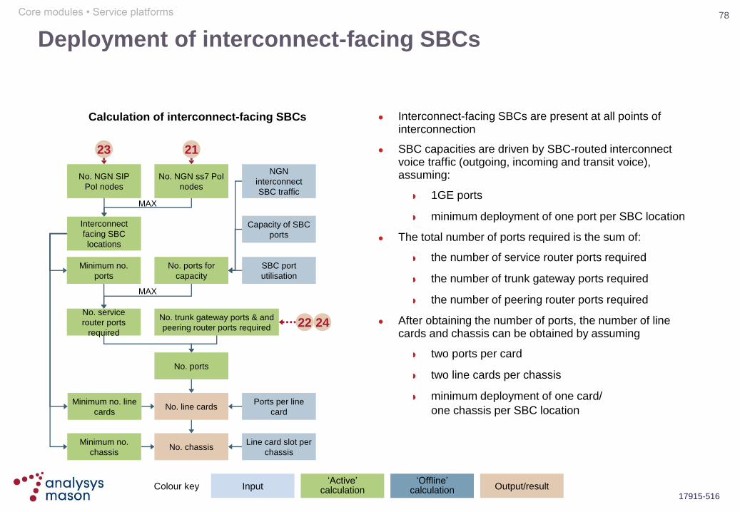
78
17915-516
Deployment of interconnect-facing SBCs
Interconnect-facing SBCs are present at all points of interconnection
SBC capacities are driven by SBC-routed interconnect voice traffic (outgoing, incoming and transit voice), assuming:
1GE ports
minimum deployment of one port per SBC location
The total number of ports required is the sum of:
the number of service router ports required
the number of trunk gateway ports required
the number of peering router ports required
After obtaining the number of ports, the number of line cards and chassis can be obtained by assuming
two ports per card
two line cards per chassis
minimum deployment of one card/
one chassis per SBC location
Calculation of interconnect-facing SBCs
No. NGN SIP
PoI nodes
No. NGN ss7 PoI
nodes
Interconnect
facing SBC
locations
MAX
NGN
interconnect
SBC traffic
Capacity of SBC
ports
SBC port
utilisation
Minimum no.
ports
No. ports for
capacity
Minimum no. line
cards
Minimum no.
chassis
No. service
router ports
required
No. trunk gateway ports & and
peering router ports required
No. ports
Ports per line
card
Line card slot per
chassis
No. line cards
No. chassis
MAX
22 24
23 21
Core modules • Service platforms
Colour key Input „Active‟
calculation Output/result „Offline‟
calculation
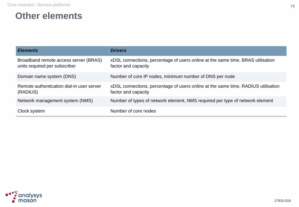
79
17915-516
Other elements
Elements Drivers
Broadband remote access server (BRAS)
units required per subscriber
xDSL connections, percentage of users online at the same time, BRAS utilisation
factor and capacity
Domain name system (DNS) Number of core IP nodes, minimum number of DNS per node
Remote authentication dial-in user server
(RADIUS)
xDSL connections, percentage of users online at the same time, RADIUS utilisation
factor and capacity
Network management system (NMS) Number of types of network element, NMS required per type of network element
Clock system Number of core nodes
Core modules • Service platforms
80
17915-516
Model overview
Market module
Overview
Access module
Core module
Network design
Access services
Service costing module
Ancillary/common/overhead modules
Introduction
Glossary

81
17915-516
The model assumes that a FTTC/VDSL network is
deployed and used to carry various NGA services
Architecture:
FTTC-VDSL technology using a new ROP is forecast to cover at least 85% of the population in
Belgium
– some locations served directly from the fibre node at the LEX/LDC without an intermediate
street cabinet
the modelled approach for copper distribution (i.e. copper between the street cabinet and the house)
is as follows: fully buried copper cables with splices; no intermediate distribution points; direct and
return copper path options
FTTO on feeder network
VoIP solution based on AGW in the ROP
Access geotyping:
dependent on the information included in BIPT‟s previous bottom-up access model and data available
at the street-cabinet level
NGA Services:
retail and wholesale end-user access - voice, DSL, Fiber To The Office (FTTO)
full and shared local loop unbundling (LLU) and sub-loop unbundling (SLU)
leased/other access lines
Access modules • Overview
82
17915-516
Some key aspects of the modelled architecture have been
modified since the industry presentation in May
We have not adopted a multiple geotype model for the access network:
instead, we have modelled the national scale deployments based upon previous BIPT calculations for
the number of kilometres of trench and cable in the feeder and distribution networks
The adopted VoIP solution is linked to the evolution of Belgacom‟s PSTN-to-VoIP (access gateway)
solution:
the active voice gateway equipment is located in the core calculation model (in the LEX/ROP)
Access modules • Overview

83
17915-516
The new model takes inputs from the bottom-up access
model built for BIPT in 2007
The bottom-up access network model developed for BIPT in 2007:
was originally developed using a detailed bottom-up design algorithm
– it calculated the volume (km and units) of copper and feeder trench, cable and splice assets
using bottom-up geo-modelling
– it was „efficient‟ in comparison to Belgacom‟s actual copper access inventory
has been updated since 2007 with asset price indexes, volumes, weighted average cost of capital
(WACC), very high bit-rate digital subscriber line (VDSL), etc.
Our bottom-up calculation takes a number of inputs from the previous access model:
efficient deployment of kilometres of trench and cable
efficient number of cable splices
starting costs for installation and equipment
We have not re-calculated a bottom-up geo-modelling of Belgacom‟s distribution and feeder network;
instead, we rely on this previous work for important deployment quantities
Access modules • Overview
84
17915-516
The access model calculates costs across the entire deployment
of network access assets for a single (long) period of operation
Belgacom‟s access network consists of network elements with generally long lifetimes:
it is sometimes hard to establish a firm lifetime because assets have yet to be replaced
– for example, some copper cables buried in the 1960s are still working (lifetime of 50+ years)
– other copper cables deployed in the year 2000 are likely to be replaced with fibre before a
50-year period is complete
– the modern equivalent asset of copper is not copper but fibre (therefore, the current – high –
price of copper does not determine the replacement cost of the entire copper network)
therefore, modelling discrete, specified asset lifetimes and replacement costs is not appropriate
Instead, the access model calculates costs across the entire deployment of network access assets for a
single (long) period of operation. This relies upon:
a roll-out profile to reach full deployment of the legacy copper access network
– plus extension of the copper network to account for long-term household growth in Belgium
a close-down profile which defines when the assets are to be retired (e.g. replaced by FTTH or
something similar)
the costs of FTTH are not modelled
This approach is best explained by the diagram on the following slide
Access modules • Overview

85
17915-516
The access module models mostly single-lifetime assets
over a full-time period: the example of copper sub-loops
Steady long-term growth in the number of households in Belgium drives the expansion of Belgacom‟s
copper network
A simple slope for the roll-out of the asset is assumed (in this case 4% deployment per annum)
It is assumed that Belgacom‟s copper network will be replaced by FTTH in the long term (2017–2037, at
5% per annum)
The actual lifetime of assets is not an input to the model, as most access assets are only deployed once
(no replacement, only maintenance)
Time 1967
Nu
mb
er
of co
pp
er
su
b-lo
op
s
2017
45–50 year asset lifetime
1991 2037
1
2 3
4
Access modules • Overview
1
2
3
4

86
17915-516
The full-period single-lifetime model is extended to other
network elements, with different roll-outs and shut-downs
Roll-out years Shut-down years Extension Notes
Copper distribution and main
distribution frame (MDF)
1967–1991 2017–2037 With household
growth
Street cabinet 1977–2003
2003–2017
2017–2037
2017–2037
Two generations of SCs are
modelled to reflect process of
replacement
Copper feeder With SCs As AGWs are
activated in the ROP
It reduces as the voice
gateway moves to ROP
Remote Optical Platform 2005–2011, then
slowly to 2015
Not shut-down It continues to be used as
FTTH is deployed
Fibre feeder With ROPs Not shut-down It is also used by other FTTO
connections
FTTO/other fibre accesses 2005–2015 Not shut-down Actual history and forecast of
FTTO/other connections
Metallic line testing With LEX
(centralised) and
SC (distributed)
With LEX and SC
Access modules • Overview
87
17915-516
The number of elements active in each year is used to
calculate capex (investment growth) and opex (expenses)
The unit capital costs (capex) for each item of equipment are sourced from the previous BRUO model.
These are separated into two parts (because of different cost trends):
installation costs (e.g. capitalised labour, deployment sub-contracts)
materials costs (cables, cabinets, hardware)
The unit operating expenses (opex) for each item are estimated using a bottom-up approach. These are
split into:
maintenance events (maintenance time, hourly manpower including allocated overheads, outsource
maintenance/contractors, additional materials)
space rental (for street cabinets and ROPs)
power and aircon (kWh power and W/m2 cooling)
Long-run cost trends determine the underlying trend in these input costs. Typically, all costs are assumed
to increase with underlying inflation. In addition, there are some specific (real-terms) trends:
installation costs around 0.5% higher than inflation, except trenching, which is around 1% higher
materials costs for SCs and ROPs are lower than inflation (by 0.8% and 0.2%, respectively)
materials costs for fibre-optic cable and the optical distribution frame (ODF) are much lower than
inflation (by 7% to 12%, respectively)
We have also increased the cost of copper cables by a total of 400% from 2004 to 2008 (see next slide)
Access modules • Overview

88
17915-516
A short-run cost trend is applied to copper cables
The short-run trend is obtained from recent observed
copper prices:
this recent trend does not reflect the long-term
trend which has been
– slowly declining in real terms since the
1960s
– approximately flat in nominal terms across
most of the years of copper deployment
Therefore, the short-run trend is applied to the materials
costs of copper, but it is not applied to the economic
depreciation of the copper investments:
this is because the recent copper cost trend does
not represent the MEA price trend (or economic
value) of copper
– the (proportional) component of line rental
did not increase by a factor of 4 from 2004
to 2008
– the price of fibre (the modern equivalent
replacement for copper) has not increased
by a factor of 4
– this recent trend is short-run only
Source: http://pubs.usgs.gov/of/2000/of00-389/of00-389.pdf
Access modules • Overview
Short-run copper price trend
Long-run copper price trend
89
17915-516
We have modelled the full lifecycle of the copper network
in order to apply depreciation over its entire lifetime
The investment costs associated with Belgacom‟s access network are recovered from the output of the
network (connected lines) over time
The copper network is not being replaced with another copper network, therefore its cost recovery should
be confined to connected copper lines
The choice of depreciation method is linked to the way in which the copper access network was deployed:
before 1997, investments were undertaken by the Belgian government
– straight-line accounting depreciation using historical book values was applicable to the business
– we assume that no return on capital was required for this period (immediately sunk investments)
– we assume that any unrecovered accounting costs were absorbed by the government
from 1997, investments were funded from capital markets
– the commercial WACC applies to cost recovery from this point onwards
– however, straight-line account was still the dominant form of cost recovery
in 2001, BIPT opened up Belgacom‟s copper access network to wholesale unbundling
from 2007, BIPT has applied cost-based access regulation, reflecting a (fully) competitive market
– cost recovery in a competitive market reflects economic depreciation (e.g. DCF)
– the remaining costs to be recovered after 2001 are treated with economic depreciation and
recovered during the remaining lifetime of the assets, from the remaining output
Access modules • Overview

90
17915-516
196
0
196
3
196
6
196
9
197
2
197
5
197
8
198
1
198
4
198
7
199
0
199
3
199
6
199
9
200
2
200
5
200
8
201
1
201
4
201
7
202
0
202
3
2026
202
9
203
2
203
5
203
8
204
1
204
4
204
7
205
0
Rea
l Te
rms u
nit c
ost
ED for all time HCA for all time HCA followed by ED
The model uses successive depreciation with different
cost recovery profiles
Historical cost accounting (HCA)-based costs show „saw-tooth‟ behaviour as large deployments take place
(with high book values); in this case we can see early copper access followed by street cabinets. Assets
tend to become fully depreciated because financial lifetimes are shorter than active lifetimes
If Economic Depreciation was applied over all time, then there would be a smooth (in real terms) trend in
the economic cost per unit of output (note: the increase in 1977 is when street cabinets are deployed)
In 2001, the cost-recovery method can move from accounting to economic costs
Accounting costs reach a minimum when many assets are fully depreciated
However, accounting costs start to rise as the number of connections decreases in later years
The assumed real-terms cost trends are very slightly increasing over time
1
2 3 4
5 6
Cost per unit of output (illustrative)
Access modules • Overview
1
2
3
4
5
6
Source: Analysys Mason

91
17915-516
Model overview
Market module
Overview
Access module
Core module
Network design
Access services
Service costing module
Ancillary/common/overhead modules
Introduction
Glossary
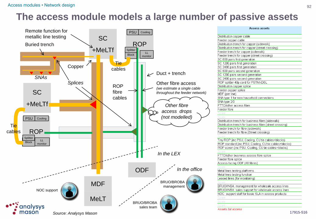
92
17915-516
SC
+MeLTf
The access module models a large number of passive assets
ROP
SC
+MeLTf
ROP
In the LEX
MDF
ODF
MeLT
Other fibre
access drops
(not modelled)
Duct + trench
Buried trench
Splices
Copper
ROP
fibre
cables
LL
monitor
LL
monitor
PSU Cooling
PSU Cooling
Block
Block
Tie
cables
Tie
cables
Remote function for
metallic line testing
Splitter
Splitter
In the office
BRUO/BROBA
sales team
BRUO/BROBA
management
Other fibre access (we estimate a single cable
throughout the feeder network)
Access modules • Network design
NOC support
SNAs
Source: Analysys Mason

93
17915-516
The calculation of expenditures works in a similar way for
all access assets
Total number of
units over time
Added units in
each year
Opex
Capex (installation
and materials)
Deployment and
drivers (roll-out and
shut-down)
Opex trends
Opex inputs
Capex trends
Capex inputs
Exceptional trends
Free extension
Colour key Input Calculations Output
Installation and
materials separately
Some trench extension is ‘free’
– paid for by the house-builder
Maintenance events (staff time and
replacement items)
Power consumption and cooling (only MeLT)
Renting space for MDF/ODF, MeLT
Number of households
Number of SCs and ROPs
FTTO and other connections
Number of LEX (for MeLT)
Access modules • Network design
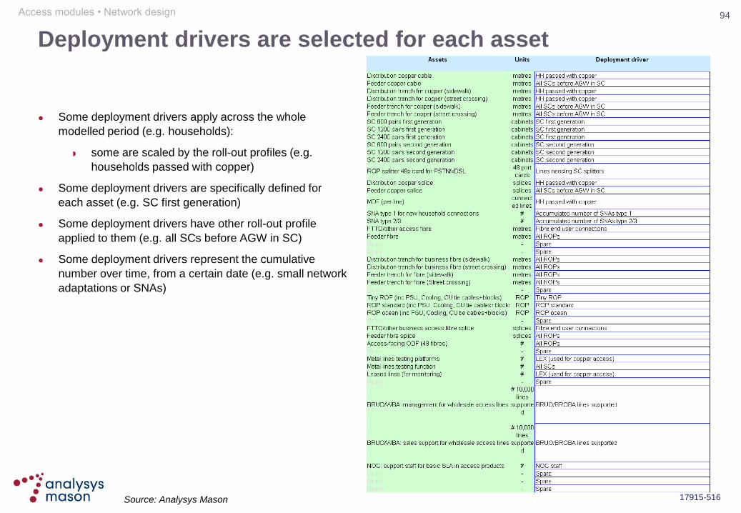
94
17915-516
Deployment drivers are selected for each asset
Some deployment drivers apply across the whole
modelled period (e.g. households):
some are scaled by the roll-out profiles (e.g.
households passed with copper)
Some deployment drivers are specifically defined for
each asset (e.g. SC first generation)
Some deployment drivers have other roll-out profile
applied to them (e.g. all SCs before AGW in SC)
Some deployment drivers represent the cumulative
number over time, from a certain date (e.g. small network
adaptations or SNAs)
Access modules • Network design
Source: Analysys Mason

95
17915-516
Cost annualisation follows a standard calculation for all
network elements
Opex
Capex (installation
and materials)
Period when HCA applies Period when economic depreciation applies
Annual opex recovery
Accounting lifetime
Depreciation plus cost
of capital employed
Capex still to be recovered
by economic
depreciation(inst+material)
Opex still to be recovered
by economic depreciation
Long-run capex
trend (inst+material)
Profile of output from
the network element
Long-run opex trend
Economic cost per unit
of output for capex
(inst+material)
Discount rate, WACC Discount rate,
WACC
Discount rate,
WACC
Economic cost per unit
of output for opex
Access modules • Network design
Colour key Input Calculations Output
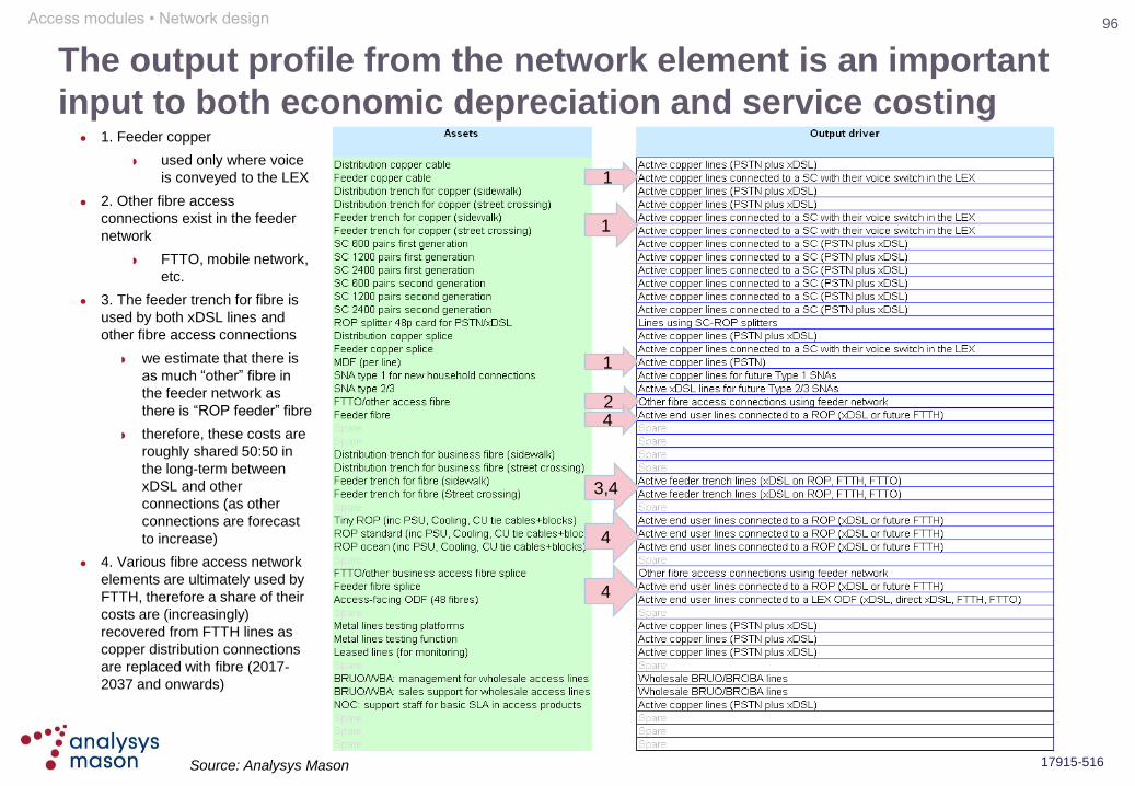
96
17915-516
Access modules • Network design
The output profile from the network element is an important
input to both economic depreciation and service costing
1
1
1
2
3,4
4
4
4
1. Feeder copper
used only where voice
is conveyed to the LEX
2. Other fibre access
connections exist in the feeder
network
FTTO, mobile network,
etc.
3. The feeder trench for fibre is
used by both xDSL lines and
other fibre access connections
we estimate that there is
as much “other” fibre in
the feeder network as
there is “ROP feeder” fibre
therefore, these costs are
roughly shared 50:50 in
the long-term between
xDSL and other
connections (as other
connections are forecast
to increase)
4. Various fibre access network
elements are ultimately used by
FTTH, therefore a share of their
costs are (increasingly)
recovered from FTTH lines as
copper distribution connections
are replaced with fibre (2017-
2037 and onwards)
Source: Analysys Mason

97
17915-516
Model overview
Market module
Overview
Access module
Core module
Network design
Access services
Service costing module
Ancillary/common/overhead modules
Introduction
Glossary
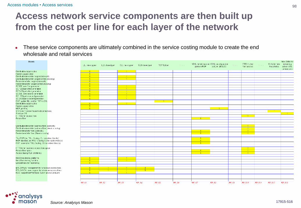
98
17915-516
Access modules • Access services
Access network service components are then built up
from the cost per line for each layer of the network
These service components are ultimately combined in the service costing module to create the end
wholesale and retail services
Source: Analysys Mason
99
17915-516
Service costing module
Model overview
Market module
Ancillary/common/overhead modules
Access module
Core module
CPE Colocation
Migration – SNA Migration – one-time fees
ISLA HMC
IT costs Overheads
Introduction
Glossary
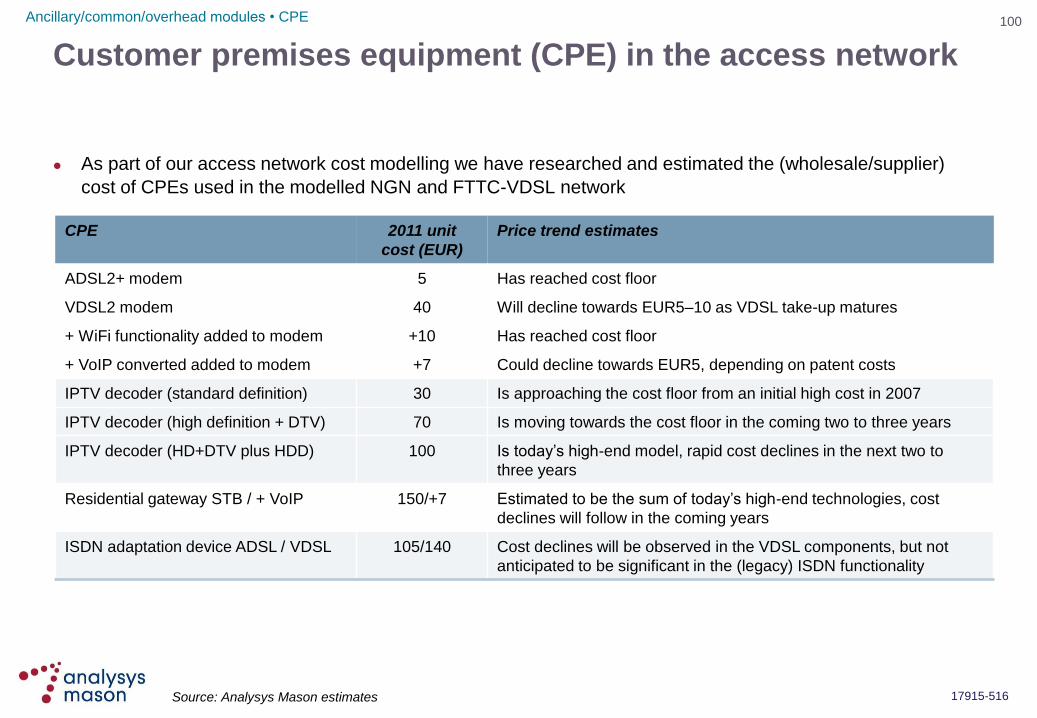
100
17915-516
Customer premises equipment (CPE) in the access network
As part of our access network cost modelling we have researched and estimated the (wholesale/supplier)
cost of CPEs used in the modelled NGN and FTTC-VDSL network
CPE 2011 unit
cost (EUR)
Price trend estimates
ADSL2+ modem 5 Has reached cost floor
VDSL2 modem 40 Will decline towards EUR5–10 as VDSL take-up matures
+ WiFi functionality added to modem +10 Has reached cost floor
+ VoIP converted added to modem +7 Could decline towards EUR5, depending on patent costs
IPTV decoder (standard definition) 30 Is approaching the cost floor from an initial high cost in 2007
IPTV decoder (high definition + DTV) 70 Is moving towards the cost floor in the coming two to three years
IPTV decoder (HD+DTV plus HDD) 100 Is today‟s high-end model, rapid cost declines in the next two to
three years
Residential gateway STB / + VoIP 150/+7 Estimated to be the sum of today‟s high-end technologies, cost
declines will follow in the coming years
ISDN adaptation device ADSL / VDSL 105/140 Cost declines will be observed in the VDSL components, but not
anticipated to be significant in the (legacy) ISDN functionality
Source: Analysys Mason estimates
Ancillary/common/overhead modules • CPE

101
17915-516
CPE Colocation
Migration – SNA Migration – one-time fees
ISLA HMC
IT costs Overheads
Service costing module
Model overview
Market module
Ancillary/common/overhead modules
Access module
Core module
Introduction
Glossary
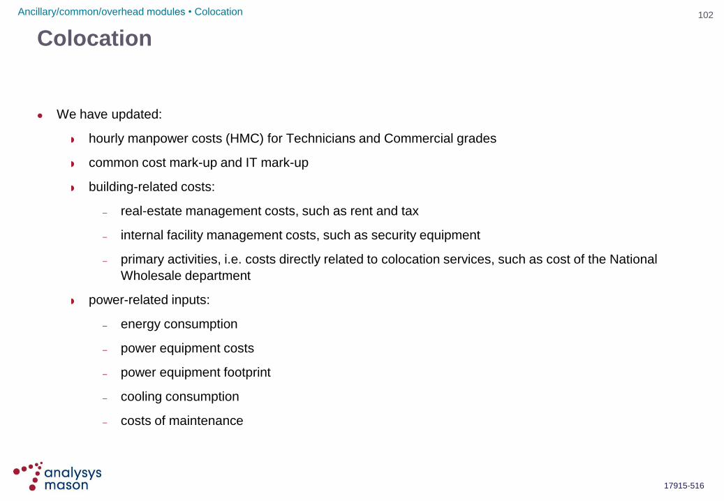
102
17915-516
Colocation
We have updated:
hourly manpower costs (HMC) for Technicians and Commercial grades
common cost mark-up and IT mark-up
building-related costs:
– real-estate management costs, such as rent and tax
– internal facility management costs, such as security equipment
– primary activities, i.e. costs directly related to colocation services, such as cost of the National
Wholesale department
power-related inputs:
– energy consumption
– power equipment costs
– power equipment footprint
– cooling consumption
– costs of maintenance
Ancillary/common/overhead modules • Colocation
103
17915-516
CPE Colocation
Migration – SNA Migration – one-time fees
ISLA HMC
IT costs Overheads
Service costing module
Model overview
Market module
Ancillary/common/overhead modules
Access module
Core module
Introduction
Glossary
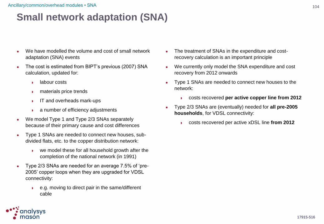
104
17915-516
Small network adaptation (SNA)
We have modelled the volume and cost of small network
adaptation (SNA) events
The cost is estimated from BIPT‟s previous (2007) SNA
calculation, updated for:
labour costs
materials price trends
IT and overheads mark-ups
a number of efficiency adjustments
We model Type 1 and Type 2/3 SNAs separately
because of their primary cause and cost differences
Type 1 SNAs are needed to connect new houses, sub-
divided flats, etc. to the copper distribution network:
we model these for all household growth after the
completion of the national network (in 1991)
Type 2/3 SNAs are needed for an average 7.5% of „pre-
2005‟ copper loops when they are upgraded for VDSL
connectivity:
e.g. moving to direct pair in the same/different
cable
The treatment of SNAs in the expenditure and cost-
recovery calculation is an important principle
We currently only model the SNA expenditure and cost
recovery from 2012 onwards
Type 1 SNAs are needed to connect new houses to the
network:
costs recovered per active copper line from 2012
Type 2/3 SNAs are (eventually) needed for all pre-2005
households, for VDSL connectivity:
costs recovered per active xDSL line from 2012
Ancillary/common/overhead modules • SNA

105
17915-516
Efficiency adjustments for SNA
BIPT‟s previous SNA cost calculation has been modified with a number of efficiency adjustments estimated
by Analysys Mason:
NTP (Network Termination Point) has been removed from Type 3 SNA
– because this upgrade aspect is not the responsibility (to be paid by) of the OLO
average pit sizes have been reduced
– because they appeared exceptionally large in our opinion
one transportation cost for Type 3 SNA
reduction of time taken to install NTP in new-build locations
– because in various cases this will be easily accomplished by the technician, or mounted by
the house-builder
Ancillary/common/overhead modules • SNA
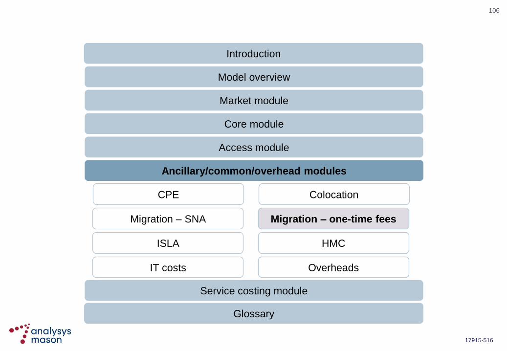
106
17915-516
CPE Colocation
Migration – SNA Migration – one-time fees
ISLA HMC
IT costs Overheads
Service costing module
Model overview
Market module
Ancillary/common/overhead modules
Access module
Core module
Introduction
Glossary

107
17915-516
One-time fees
We have updated:
the WACC
HMC for Technicians and Commercial grades
travel time based on indirect costs associated with network utility time
indirect NWS/CCA(1) staff in addition to minuted direct staff
mark-up formula for NWS/CCA staff (correction)
common cost mark-up and IT mark-up
equipment costs
We have estimated CPS (carrier pre select) connection activity costs
In some cases, the calculated costs go down (lower mark-ups, lower indirect staff)
In other cases, the calculated costs go up (HMC overheads as an hourly standard increases the hourly cost
of lower-grade staff more than the previous 6% equi-proportional mark-up (EPMU))
Some of the (many) inputs to the one-time fee calculations appear odd or potentially excessive to us. These
aspects will be tested in consultation
Ancillary/common/overhead modules • One-time fees
(1)Existing staff grade in one-time fee model

108
17915-516
CPE Colocation
Migration – SNA Migration – one-time fees
ISLA HMC
IT costs Overheads
Service costing module
Model overview
Market module
Ancillary/common/overhead modules
Access module
Core module
Introduction
Glossary
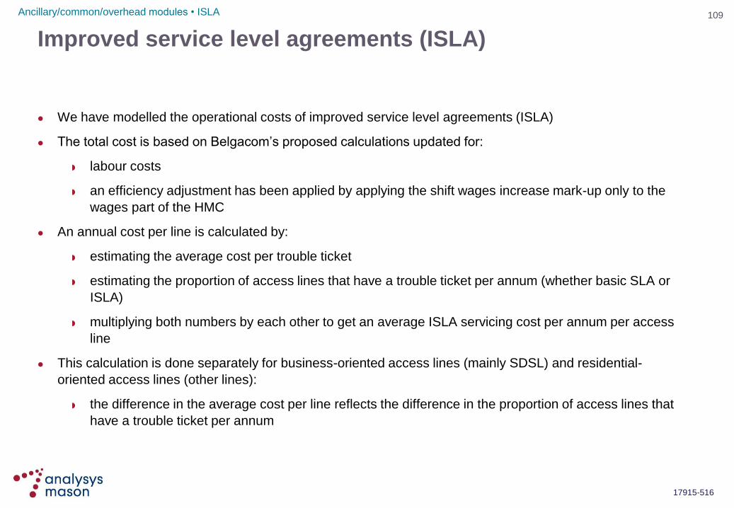
109
17915-516
Improved service level agreements (ISLA)
We have modelled the operational costs of improved service level agreements (ISLA)
The total cost is based on Belgacom‟s proposed calculations updated for:
labour costs
an efficiency adjustment has been applied by applying the shift wages increase mark-up only to the
wages part of the HMC
An annual cost per line is calculated by:
estimating the average cost per trouble ticket
estimating the proportion of access lines that have a trouble ticket per annum (whether basic SLA or
ISLA)
multiplying both numbers by each other to get an average ISLA servicing cost per annum per access
line
This calculation is done separately for business-oriented access lines (mainly SDSL) and residential-
oriented access lines (other lines):
the difference in the average cost per line reflects the difference in the proportion of access lines that
have a trouble ticket per annum
Ancillary/common/overhead modules • ISLA

110
17915-516
CPE Colocation
Migration – SNA Migration – one-time fees
ISLA HMC
IT costs Overheads
Service costing module
Model overview
Market module
Ancillary/common/overhead modules
Access module
Core module
Introduction
Glossary

111
17915-516
Module 15: hourly manpower costs (HMC) for network
activities
An organisation the size of Belgacom has a large number of network staff involved in the design,
deployment, installation, maintenance, operation and management of the network
The average hourly wage rate for Belgacom‟s network engineers is:
EURxx per hour (calculated from an average 2009 salary of EURxx 000 per annum, based on 1725
working hours per annum)
– a proportion of these hours (xx% according to Belgacom, 10% according to Analysys Mason
estimates) are in training, breaks, absence, etc.
– according to the European Working Conditions Observatory*, sickness absence in Belgium is
considered high (approximately five days sick per annum, plus two other days absence = 3% of
working days)
In addition, outsourced labour and maintenance contracts are in place:
some of these outsource contracts cover explicit non-HMC costs (e.g. outsourced SNA work,
outsourced power contracts added to colocation equipment)
Remaining un-allocated outsourced contracts amount to:
an additional xx% (EURxx per hour) for Belgacom‟s passive network elements
an additional xx% (EURxx per hour) for Belgacom‟s active network equipment
an additional xx% for (EURxx per hour) civil works and road digging
* http://www.eurofound.europa.eu/ewco/studies/tn0911039s/be0911039q.htm
Ancillary/common/overhead modules • HMC

112
17915-516
Module 15: indexing HMC
Hourly wage calculations refer to year 2009:
Belgacom has submitted the indexing formula which it is legally obliged to follow
Belgacom also increases all wages by a merit index. We do not apply this merit index on the long-run
cost base of Belgacom (even if it is routinely applied to retained individuals‟ salaries)
excluding the merit index, the nominal wage index is approximately inflationary, and equal to:
– 2009–2010 = 0.5%
– 2010–2011 = 2.68%
– 2011–2012 = 2.34%
Ancillary/common/overhead modules • HMC

113
17915-516
CPE Colocation
Migration – SNA Migration – one-time fees
ISLA HMC
IT costs Overheads
Service costing module
Model overview
Market module
Ancillary/common/overhead modules
Access module
Core module
Introduction
Glossary

114
17915-516
Module 16: IT costs
For an operator the size of Belgacom, the IT
department consists of:
around xxx servers (e.g. mix of mainframe,
Windows, Linux)
xxx IT support staff, excluding developers
(admin, monitoring, operations and
maintenance, planning, management)
Annualised costs of the IT department are around
EURxxx million
This covers:
all server hardware (four-year assets)
development software (annualised cost)
IT support staff direct costs
– EURxx wages per hour
(EURxx 000 salary)
– plus expensed tools/vehicles
consultancy and maintenance contracts
IT functions have been split according to
Belgacom‟s activities
The overall allocation of IT costs is shown opposite
Retail
xx%
Overheads
xx%
Network
xx%
(which splits
as shown):
All assets
x%
Consumer
services
x%
Carrier
services
x%
(LL, BRUO,
IC including
internal
operator
services) This EURxx million direct to wholesale
and internal services, based on a number of
carrier services (e.g. LL, VPN, BRUO,
BRIO, WBA, CPS)
This EURxx million to
overheads allocation
Ancillary/common/overhead modules • IT costs
Source: Analysys Mason analysis of Belgacom data
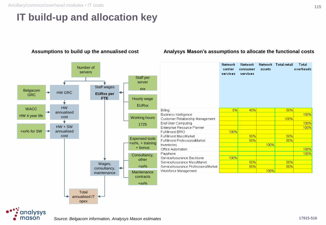
115
17915-516
IT build-up and allocation key
HW GRC
HW
annualised
cost
WACC
HW 4 year life
HW + SW
annualised
cost
+xx% for SW
Staff per
server
xxx
Hourly wage
EURxx
Working hours
1725
Staff wages
EURxx per
FTE
Consultancy,
other
+xx%
Maintenance
contracts
+xx%
Number of
servers
Wages,
consultancy,
maintenance
Total
annualised IT
opex
Assumptions to build up the annualised cost Analysys Mason’s assumptions to allocate the functional costs
Source: Belgacom information, Analysys Mason estimates
Belgacom
GRC
Expensed tools
+xx%, + training
+ bonus
Ancillary/common/overhead modules • IT costs

116
17915-516
Calculation of IT mark-ups
Based on the total IT service annualised costs (around EURxxx million) and the allocation keys, a
proportion of IT costs are calculated to be relevant for:
all network assets
network consumer services (e.g. retail voice and broadband)
network carrier services (e.g. leased lines, BRUO, internal services)
We have used Belgacom‟s regulatory accounts to estimate the total annualised cost applying to the service
delivery engine (network and IT). From this, we have calculated the percentage mark-up to network costs:
for all network assets: +x% applicable to all network services
for consumer services: +x% applicable only to consumer services (i.e. x% in total)
for carrier services: +x% applicable to wholesale and other carrier services (i.e. x% in total)
Ancillary/common/overhead modules • IT costs

117
17915-516
CPE Colocation
Migration – SNA Migration – one-time fees
ISLA HMC
IT costs Overheads
Service costing module
Model overview
Market module
Ancillary/common/overhead modules
Access module
Core module
Introduction
Glossary

118
17915-516
Module 17: overheads and additional staff costs
Hourly staff costs for IT and network functions have been identified:
EURxx per hour for IT staff
EURxx per hour for network engineers
Belgacom also incurs the following costs:
wage benefits: pension, bonus, training, medicals
– +xx% (comprising xx% pension back service (excluded in BU), xx% collective bonus and xx%
training/medical costs)
– the pension back service is currently excluded
expensed tools and vehicles
– we estimate that this mark-up is different for the types of network activities (xx% on average)
– +xx% within the network department for utility work (this includes vehicle-related tools)
– +x% within the network department for „desk-based‟ work
office space rental
– separate space-based calculation
Ancillary/common/overhead modules • Overheads
Source: Belgacom information
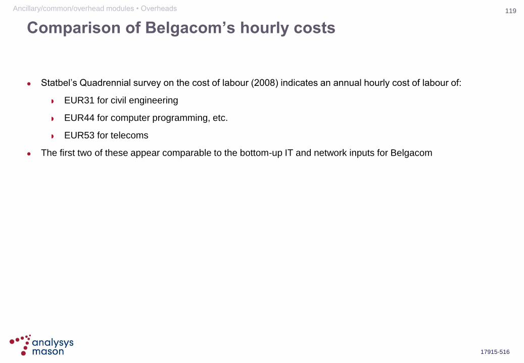
119
17915-516
Comparison of Belgacom’s hourly costs
Statbel‟s Quadrennial survey on the cost of labour (2008) indicates an annual hourly cost of labour of:
EUR31 for civil engineering
EUR44 for computer programming, etc.
EUR53 for telecoms
The first two of these appear comparable to the bottom-up IT and network inputs for Belgacom
Ancillary/common/overhead modules • Overheads
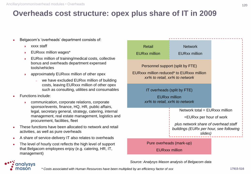
120
17915-516
Overheads cost structure: opex plus share of IT in 2009
Belgacom‟s „overheads‟ department consists of:
xxxx staff
EURxxx million wages*
EURxx million of training/medical costs, collective
bonus and overheads department expensed
tools/vehicles
approximately EURxxx million of other opex
– we have excluded EURxx million of building
costs, leaving EURxxx million of other opex
such as consulting, utilities and consumables
Functions include:
communication, corporate relations, corporate
sponsor/events, finance, HQ, HR, public affairs,
legal, secretary general, strategy, catering, internal
management, real estate management, logistics and
procurement, facilities, fleet
These functions have been allocated to network and retail
activities, as well as pure overheads
A share of service-delivery IT also relates to overheads
The level of hourly cost reflects the high level of support
that Belgacom employees enjoy (e.g. catering, HR, IT,
management)
Network total = EURxxx million
=EURxx per hour of work
plus network share of overhead staff
buildings (EURx per hour, see following
slides)
Retail
EURxx million
Pure overheads (mark-up)
EURxxx million
Network
EURxx million
Personnel support (split by FTE)
EURxxx million reduced* to EURxxx million
xx% to retail, xx% to network
IT overheads (split by FTE)
EURxx million
xx% to retail, xx% to network
* Costs associated with Human Resources have been multiplied by an efficiency factor of xxx
Ancillary/common/overhead modules • Overheads
Source: Analysys Mason analysis of Belgacom data

121
17915-516
Overheads cost structure: rent per square metre
In addition to the overheads opex, there is:
EURxx million of building costs (rent, taxes, other)
EURxx million of annualised FIX+FITTINGS
investments
EURxxx million of annualised building investments
– EURxx million estimated to cover owned
buildings (e.g. including Heverlee and
Schaerbeek of at least xxx 000 square
metres)
– around EURxx million of improvements
– plus around EURxx million for energy/
aircon, etc. in various technical buildings
These costs appear to cover the entire building estate of
Belgacom
Within these buildings sit the overheads, IT, network and
retail personnel, plus network equipment, catering, etc.
A total space per full-time employee (FTE) of around
xx–xx square metre means that total employees occupy
xxx 000 square metres:
of which xx square metres is for office space per
person
Typical office space allocations range from:
12.5 square metres for personal space only
to 25 square metres for rentable space per
employee
Parking allocations of around xx–xx square metres reflect
around one space per employee
Based on more efficient space allocations, and less than
one parking space per employee, it appears reasonable
to reduce space per FTE from xx square metres to a total
of 27.5 square metres:
with an annual rent of EURxx per square metres
plus 7.5% property taxes
Ancillary/common/overhead modules • Overheads
122
17915-516
Overheads and buildings: improvements and power/aircon
Fixtures, fittings and building improvements add EURxx million on around EURxx million of rent:
+xxx% mark-up per square metre to all space
We have estimated that other building costs (e.g. electricity) are higher within technical buildings than office
accommodation:
EURxx million of other building costs split into EURxx million technical and EURxx million office
Power/aircon annualised costs add around EURxx million on technical space rent (which is about xx% of
the total space):
+xxx% mark-up per square metre to technical space
Resulting costs per square metre:
EURxxx per square metre for fitted out, powered and supported office space
EURxxx per square metre for technical space including all power/aircon equipment and consumption
Office space is converted into an hourly cost per FTE and added into the hourly manpower costs (HMC) for
network and overhead activities
Ancillary/common/overhead modules • Overheads
123
17915-516
Model overview
Market module
Ancillary/common/overhead modules
Access module
Core module
Service costing module
Introduction
Glossary

124
17915-516
The service costing module contains the main scenario
and model controls …
Service costing module
Source: BIPT model v1.0
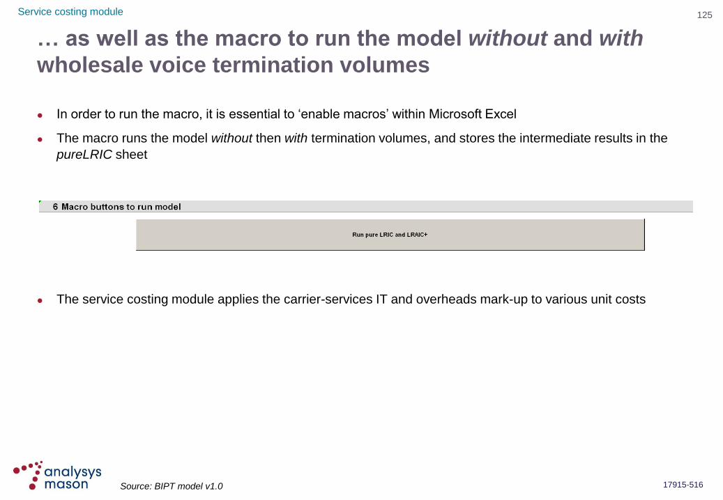
125
17915-516
… as well as the macro to run the model without and with
wholesale voice termination volumes
In order to run the macro, it is essential to „enable macros‟ within Microsoft Excel
The macro runs the model without then with termination volumes, and stores the intermediate results in the
pureLRIC sheet
The service costing module applies the carrier-services IT and overheads mark-up to various unit costs
Service costing module
Source: BIPT model v1.0

126
17915-516
The cost of the end-to-end wholesale services are built up
from the various calculated cost components
Service costing module
Source: BIPT model v1.0
127
17915-516
Model overview
Market module
Ancillary/common/overhead modules
Access module
Core module
Service costing module
Introduction
Glossary
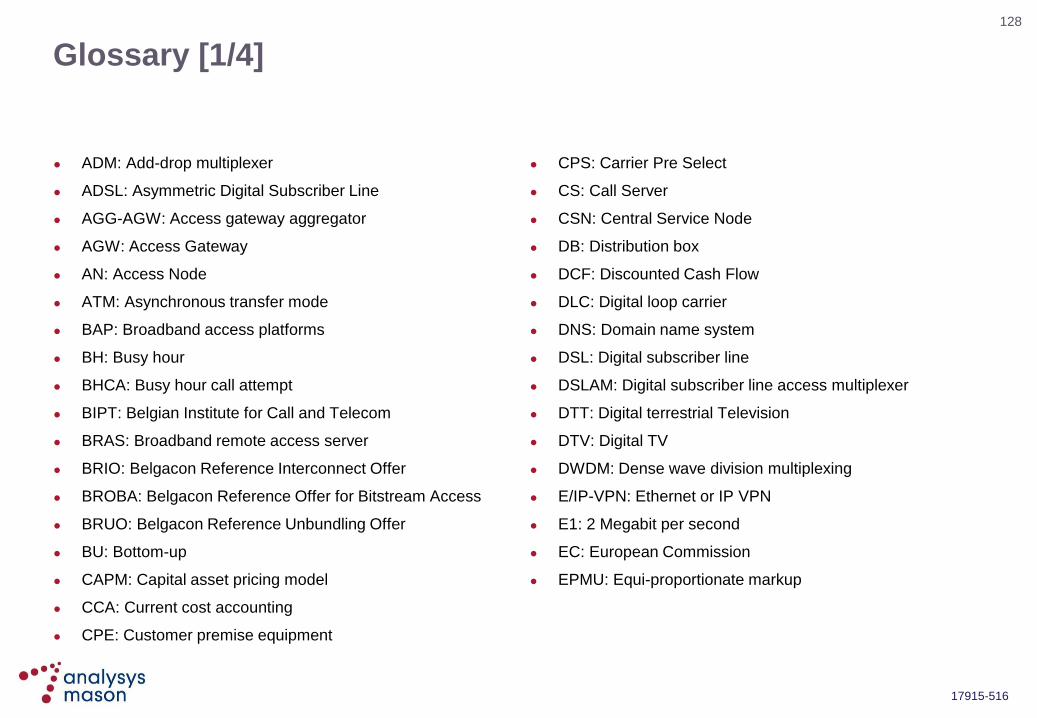
128
17915-516
Glossary [1/4]
ADM: Add-drop multiplexer
ADSL: Asymmetric Digital Subscriber Line
AGG-AGW: Access gateway aggregator
AGW: Access Gateway
AN: Access Node
ATM: Asynchronous transfer mode
BAP: Broadband access platforms
BH: Busy hour
BHCA: Busy hour call attempt
BIPT: Belgian Institute for Call and Telecom
BRAS: Broadband remote access server
BRIO: Belgacon Reference Interconnect Offer
BROBA: Belgacon Reference Offer for Bitstream Access
BRUO: Belgacon Reference Unbundling Offer
BU: Bottom-up
CAPM: Capital asset pricing model
CCA: Current cost accounting
CPE: Customer premise equipment
CPS: Carrier Pre Select
CS: Call Server
CSN: Central Service Node
DB: Distribution box
DCF: Discounted Cash Flow
DLC: Digital loop carrier
DNS: Domain name system
DSL: Digital subscriber line
DSLAM: Digital subscriber line access multiplexer
DTT: Digital terrestrial Television
DTV: Digital TV
DWDM: Dense wave division multiplexing
E/IP-VPN: Ethernet or IP VPN
E1: 2 Megabit per second
EC: European Commission
EPMU: Equi-proportionate markup

129
17915-516
Glossary [2/4]
FAC: Fully-allocated cost
FAR: Fixed asset register
FTE: Full time equivalent
FTTC: Fibre-to-the-cabinet
FTTH: Fibre-to-the-home
FTTN: Fibre-to-the-node
FTTO: Fibre-to-the-office
GE: Gigabit Ethernet
GPON: Gigabit passive optical network
HD: High definition
HDD: Hard Disk Drive
HMC: Hourly manpower cost
IGE: International gateway
IP: Internet protocol
IP BAP: IP Broadband Access Platform
IPTV: Internet protocol television
ISDN: Integrated services digital network
ISDN-2: ISDN Basic Rate Interface
ISDN-30: ISDN Primary Rate Interface
ISLA: Improved Service Level Agreement
ISP: Internet Service Provider
IT: Information technology
LAN: Local Area Network
LDC: Local Distribution Cabinets
LEX: Local Exchange
LEX-AGW: AGW located in the LEX
LL: Leased Line
LLU: Local loop unbundling
LN: Local node
LRAIC: Long-run average incremental cost
LRIC: Long-run incremental cost
LS: Local switch
MDF: Main distribution frame
MEA: Modern equivalent asset
MeLT: Metallic line testing
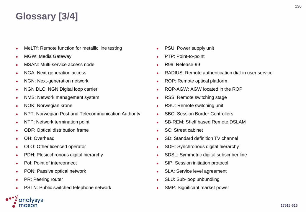
130
17915-516
Glossary [3/4]
MeLTf: Remote function for metallic line testing
MGW: Media Gateway
MSAN: Multi-service access node
NGA: Next-generation access
NGN: Next-generation network
NGN DLC: NGN Digital loop carrier
NMS: Network management system
NOK: Norwegian krone
NPT: Norwegian Post and Telecommunication Authority
NTP: Network termination point
ODF: Optical distribution frame
OH: Overhead
OLO: Other licenced operator
PDH: Plesiochronous digital hierarchy
PoI: Point of interconnect
PON: Passive optical network
PR: Peering router
PSTN: Public switched telephone network
PSU: Power supply unit
PTP: Point-to-point
R99: Release-99
RADIUS: Remote authentication dial-in user service
ROP: Remote optical platform
ROP-AGW: AGW located in the ROP
RSS: Remote switching stage
RSU: Remote switching unit
SBC: Session Border Controllers
SB-REM: Shelf based Remote DSLAM
SC: Street cabinet
SD: Standard definition TV channel
SDH: Synchronous digital hierarchy
SDSL: Symmetric digital subscriber line
SIP: Session initiation protocol
SLA: Service level agreement
SLU: Sub-loop unbundling
SMP: Significant market power

131
17915-516
Glossary [4/4]
SN: Service Node
SNA: Small network adaptation
SR: Service router
SS7: Signalling system 7
STB: Set top box
TD: Top-down
TDM: Time division multiplexing
TGW: Transit media gateway; trunk gateway
TSP: Travelling Salesman Problem
VDSL: Very high-rate Digital Subscriber Line
VoB: Voice-over-broadband
VoD: Video-on-demand
VoIP: Voice over internet protocol
VPN: Virtual private network
WACC: Weighted average cost of capital
xDSL: Generic term for DSL

132
17915-516
Ian Streule
Gilles Monniaux
Analysys Mason Limited
St Giles Court, 24 Castle Street
Cambridge CB3 0AJ, UK
Tel: +44 (0)845 600 5244
Fax: +44 (0)1223 460866
www.analysysmason.com
Registered in England No. 5177472
Stéphane Piot
Pierre Fortier
Analysys Mason Limited
St Giles Court, 24 Castle Street
Cambridge CB3 0AJ, UK
Tel: +44 (0)845 600 5244
Fax: +44 (0)1223 460866
www.analysysmason.com
Registered in England No. 5177472