Finding the Oddballs

Adam Ashenfelter (ashenfelter@bigml.com)

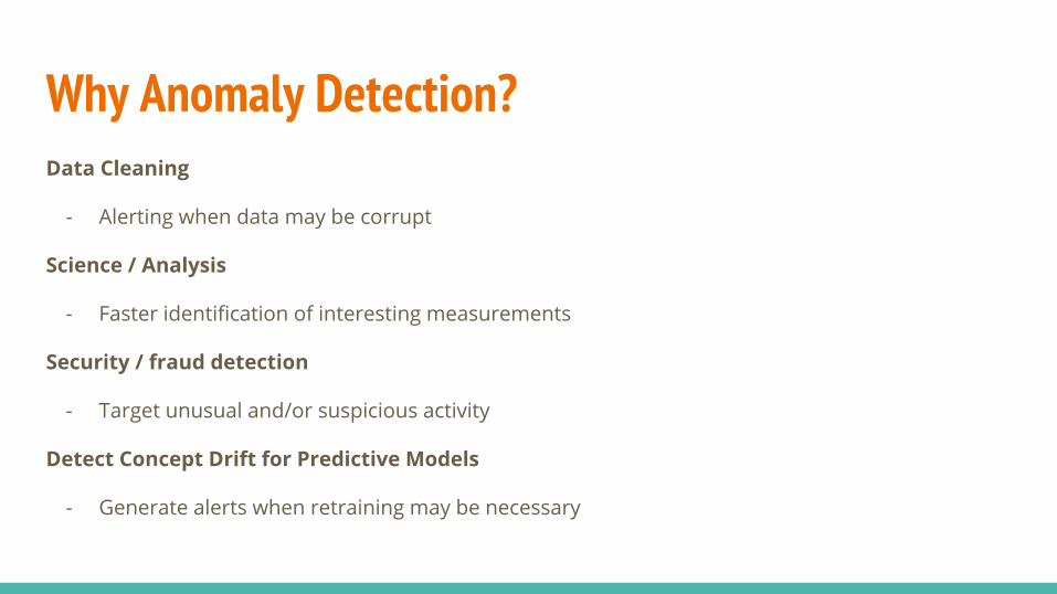
Why Anomaly Detection?Data Cleaning

- Alerting when data may be corrupt

Science / Analysis

- Faster identification of interesting measurements

Security / fraud detection

- Target unusual and/or suspicious activity

Detect Concept Drift for Predictive Models

- Generate alerts when retraining may be necessary

DARPA ADAMS ProjectDesktop activity collected from ~5000 employees of a corporation using Raytheon-Oakley’s Sureview

Insider threat scenarios overlaid on selected employees:

● Anomalous Encryption● Layoff Logic Bomb● Insider Startup● Circumventing SureView

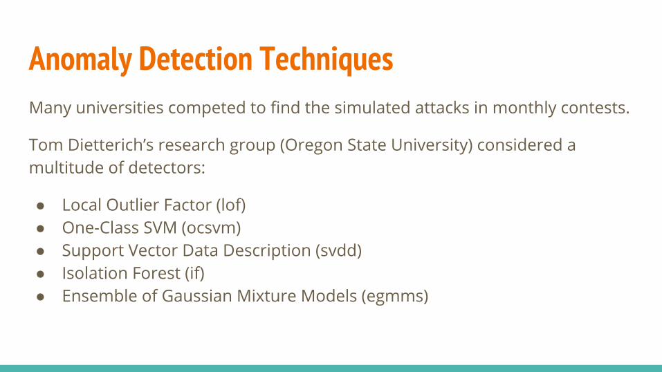
Anomaly Detection TechniquesMany universities competed to find the simulated attacks in monthly contests.

Tom Dietterich’s research group (Oregon State University) considered a multitude of detectors:

● Local Outlier Factor (lof)● One-Class SVM (ocsvm)● Support Vector Data Description (svdd)● Isolation Forest (if)● Ensemble of Gaussian Mixture Models (egmms)

Lack of Public Anomaly Detection DatasetsMost anomaly detection datasets are proprietary and/or classified.

No equivalent of the UCI supervised learning dataset collection.

How can we rigorously compare all these detection techniques in a repeatable manner?

Let’s transform supervised learning datasets!

A. Emmott, et al. Systematic Construction of Anomaly Detection Benchmarks. ODD Workshop, 2013

Support Vector Machine TechniquesOne-Class SVM

Shifts data from the origin with and searches for a hyper-plane which separates the majority of the data from the origin.

B. Scholkopf, et al. Estimating the support of a high-dimensional distribution, 1999

Available in libsvm, R, and SciKit Learn.

Support Vector Data Description

Finds the smallest hyper-sphere (in kernel space) that separates most of the data

Tax and Duin. Support vector data description. Machine Learning, 2004

Available in libsvmtools.

Support Vector Machine Techniques

Support Vector Machine Techniques

Support Vector Machine Techniques

Support Vector Machine Techniques

Support Vector Machine Techniques

Support Vector Machine Techniques

Compute the average distance from the each point to its closest neighbors as an estimate of the inverse density.

For each point, calculate:

M. Breunig, et al. LOF: identifying density-based local outliers. ACM SIGMOD Record, 2000

Available in R.

Local Outlier Factor

average density of neighbor points

current point’s density

Compute the average distance from the each point to its closest neighbors as an estimate of the inverse density.

For each point, calculate:

M. Breunig, et al. LOF: identifying density-based local outliers. ACM SIGMOD Record, 2000

Available in R.

Local Outlier Factor

average density of neighbor points

current point’s density

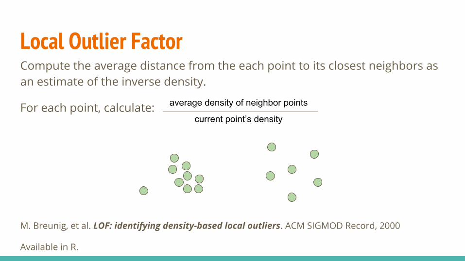
Compute the average distance from the each point to its closest neighbors as an estimate of the inverse density.

For each point, calculate:

M. Breunig, et al. LOF: identifying density-based local outliers. ACM SIGMOD Record, 2000

Available in R.

Local Outlier Factor

average density of neighbor points

current point’s density

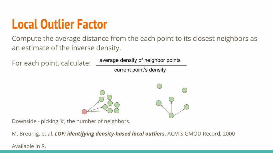
Compute the average distance from the each point to its closest neighbors as an estimate of the inverse density.

For each point, calculate:

Downside - picking ‘k’, the number of neighbors.

M. Breunig, et al. LOF: identifying density-based local outliers. ACM SIGMOD Record, 2000

Available in R.

Local Outlier Factor

average density of neighbor points

current point’s density

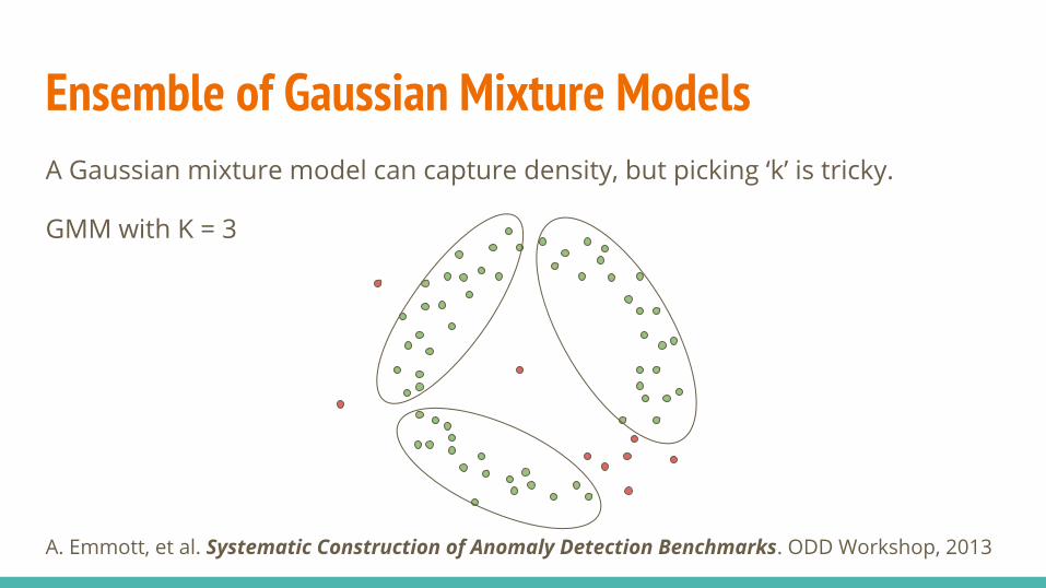
A Gaussian mixture model can capture density, but picking ‘k’ is tricky.

GMM with K = 3

A. Emmott, et al. Systematic Construction of Anomaly Detection Benchmarks. ODD Workshop, 2013

Ensemble of Gaussian Mixture Models

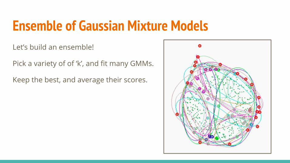
Ensemble of Gaussian Mixture ModelsLet’s build an ensemble!

Pick a variety of of ‘k’, and fit many GMMs.

Keep the best, and average their scores.

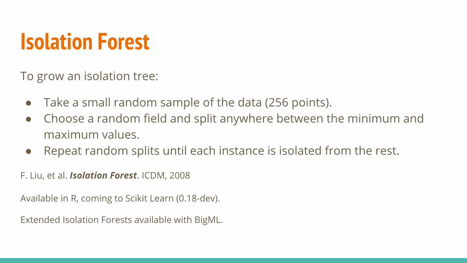
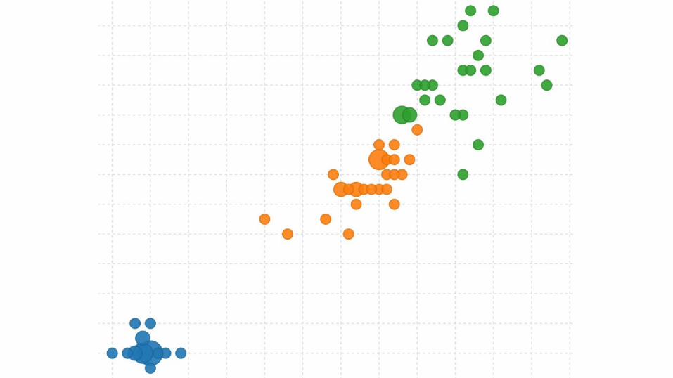
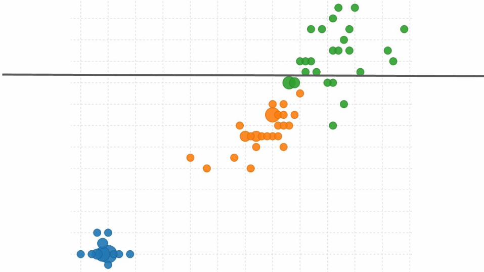
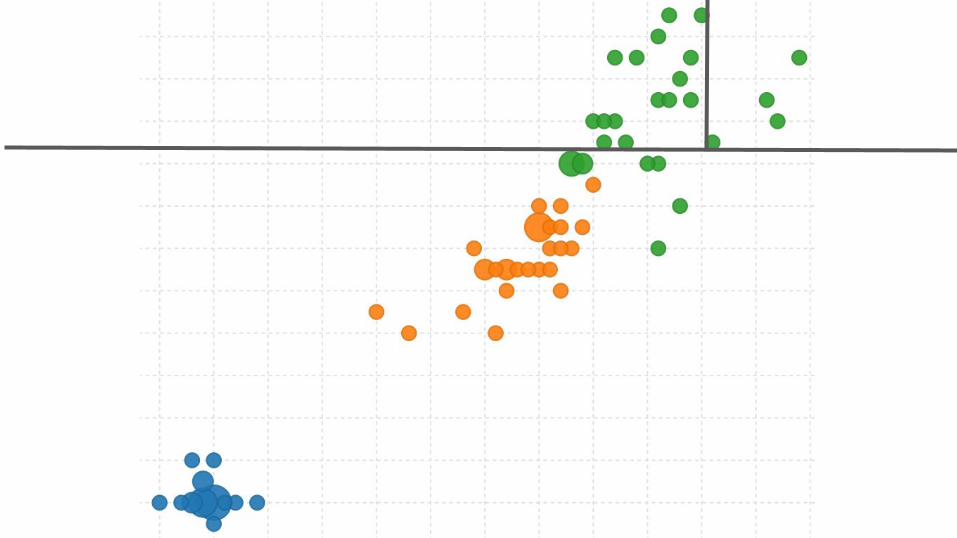
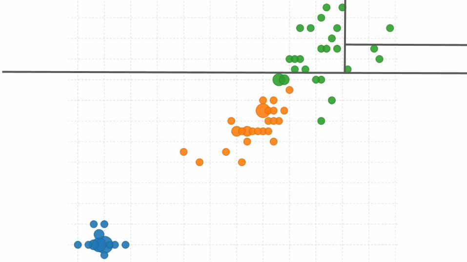
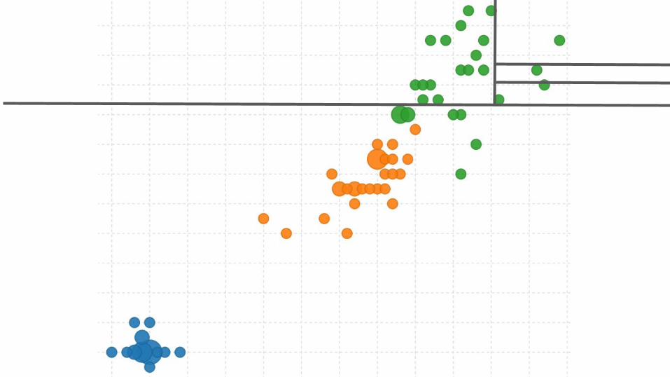
Isolation ForestTo grow an isolation tree:

● Take a small random sample of the data (256 points).● Choose a random field and split anywhere between the minimum and

maximum values.● Repeat random splits until each instance is isolated from the rest.

F. Liu, et al. Isolation Forest. ICDM, 2008

Available in R, coming to Scikit Learn (0.18-dev).

Extended Isolation Forests available with BigML.

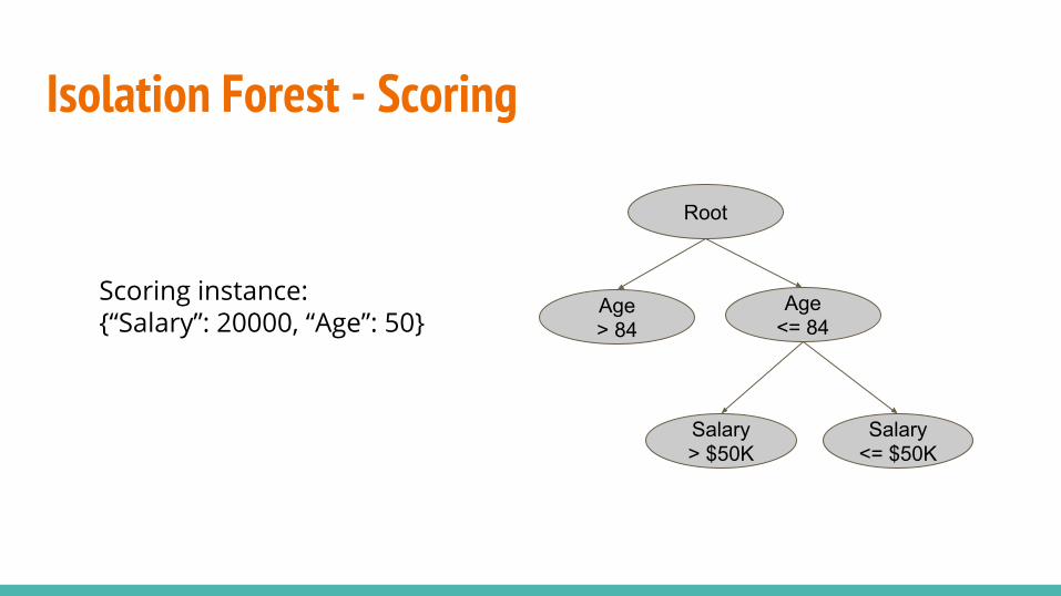
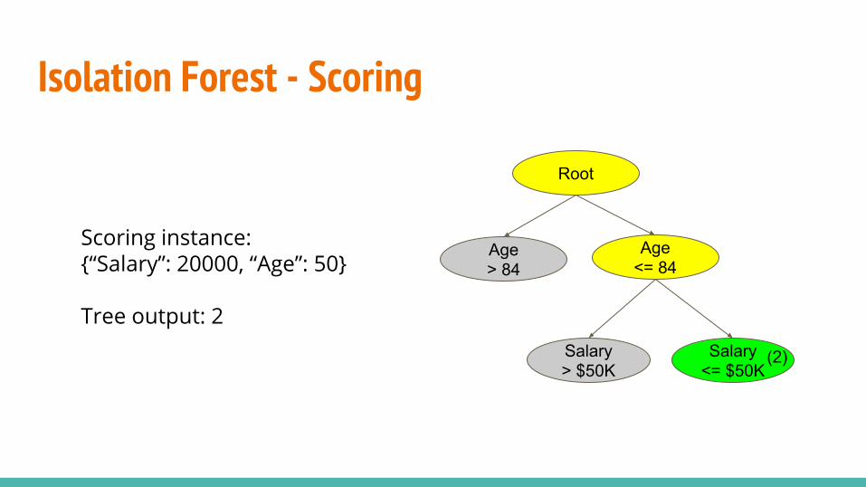
Isolation Forest - Scoring

Age<= 84

Salary> $50K

Salary<= $50K

Scoring instance:{“Salary”: 20000, “Age”: 50}

Root

Age> 84

Isolation Forest - Scoring

Age<= 84

Salary> $50K

Salary<= $50K

Scoring instance:{“Salary”: 20000, “Age”: 50}

Tree output: 2

Root

Age> 84

(2)

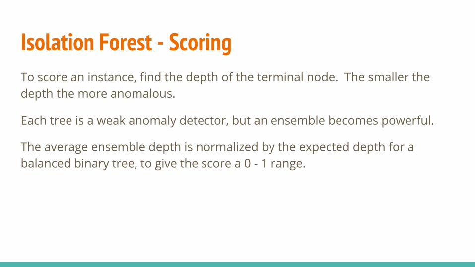
Isolation Forest - ScoringTo score an instance, find the depth of the terminal node. The smaller the depth the more anomalous.

Each tree is a weak anomaly detector, but an ensemble becomes powerful.

The average ensemble depth is normalized by the expected depth for a balanced binary tree, to give the score a 0 - 1 range.

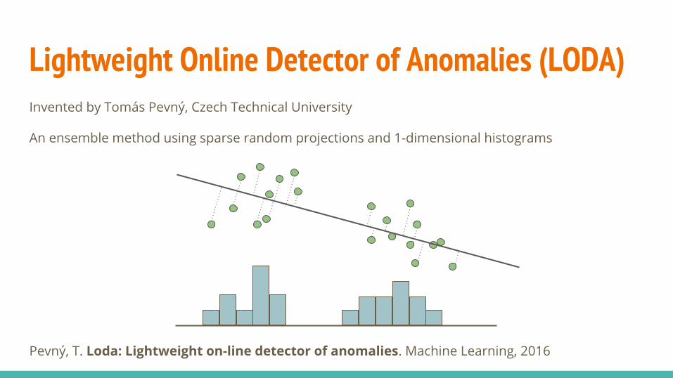
Lightweight Online Detector of Anomalies (LODA)Invented by Tomás Pevný, Czech Technical University

An ensemble method using sparse random projections and 1-dimensional histograms

Pevný, T. Loda: Lightweight on-line detector of anomalies. Machine Learning, 2016

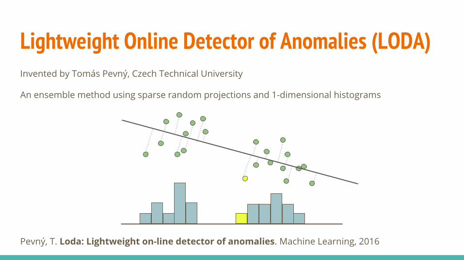
Lightweight Online Detector of Anomalies (LODA)Invented by Tomás Pevný, Czech Technical University

An ensemble method using sparse random projections and 1-dimensional histograms

Pevný, T. Loda: Lightweight on-line detector of anomalies. Machine Learning, 2016

Lightweight Online Detector of Anomalies (LODA)Another ensemble method - weak individually but powerful in numbers.

Can operate as an on-line anomaly detector when paired with streaming histograms (see https://github.com/bigmlcom/histogram).

When operating in batch mode, LODA is often competitive with Isolation Forests.

Scales nicely to wide datasets.

Blazingly fast to train and score!

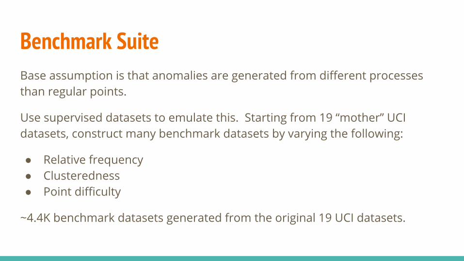
Benchmark SuiteBase assumption is that anomalies are generated from different processes than regular points.

Use supervised datasets to emulate this. Starting from 19 “mother” UCI datasets, construct many benchmark datasets by varying the following:

● Relative frequency● Clusteredness● Point difficulty

~4.4K benchmark datasets generated from the original 19 UCI datasets.

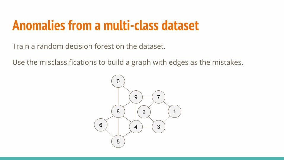
Anomalies from a multi-class dataset Train a random decision forest on the dataset.

Use the misclassifications to build a graph with edges as the mistakes.

9

8

7

6

5

4 3

2 1

0

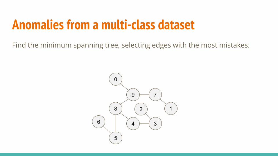
Anomalies from a multi-class dataset Find the minimum spanning tree, selecting edges with the most mistakes.

9

8

7

6

5

4 3

2 1

0

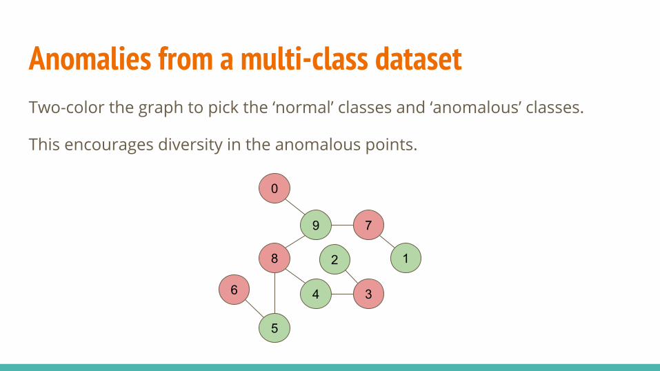
Anomalies from a multi-class dataset Two-color the graph to pick the ‘normal’ classes and ‘anomalous’ classes.

This encourages diversity in the anomalous points.

9

8

7

6

5

4 3

2 1

0

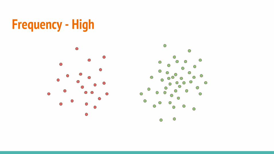
Frequency - High

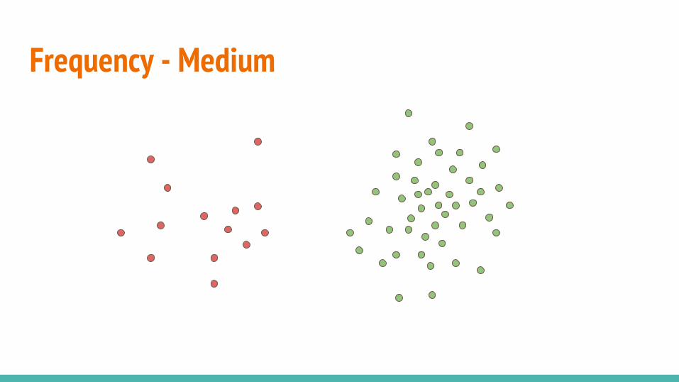
Frequency - Medium

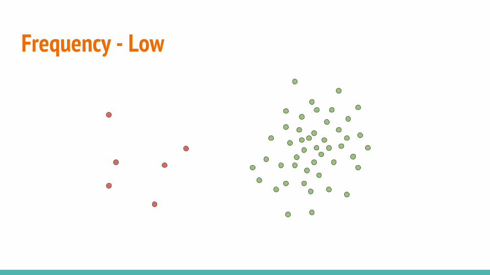
Frequency - Low

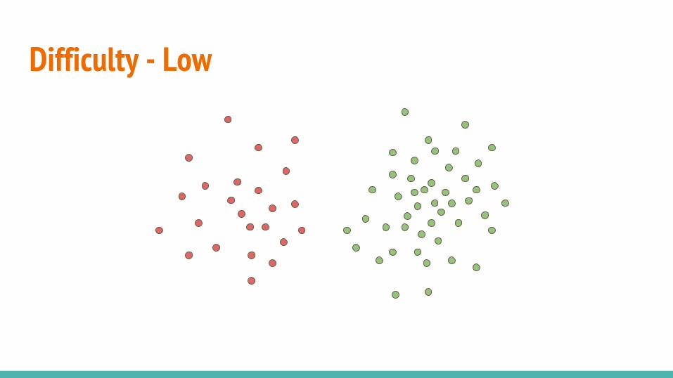
Difficulty - Low

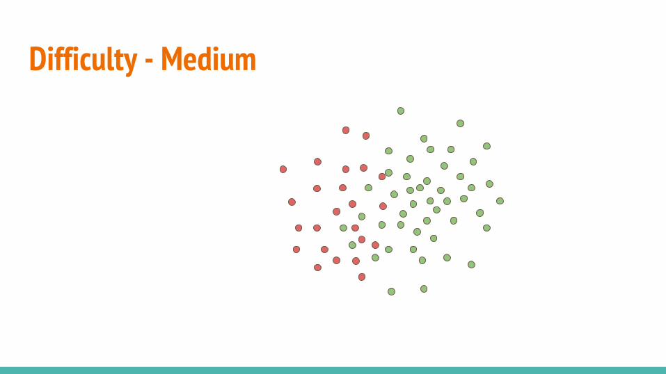
Difficulty - Medium

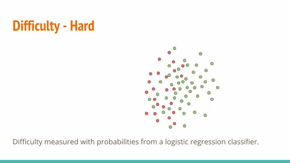
Difficulty - Hard

Difficulty measured with probabilities from a logistic regression classifier.

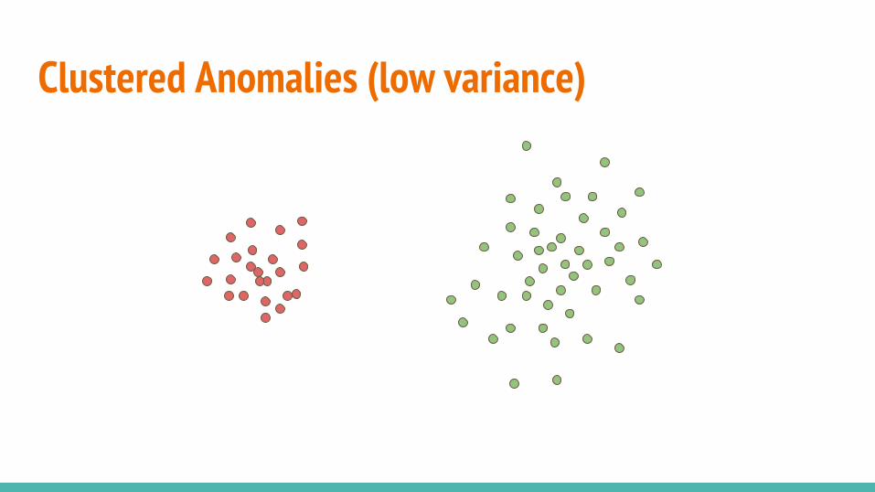
Clustered Anomalies (low variance)

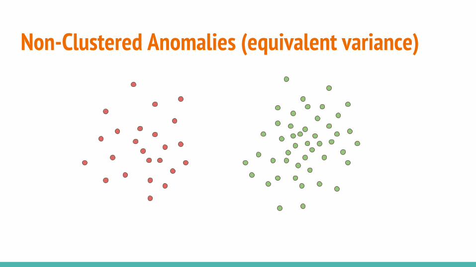
Non-Clustered Anomalies (equivalent variance)

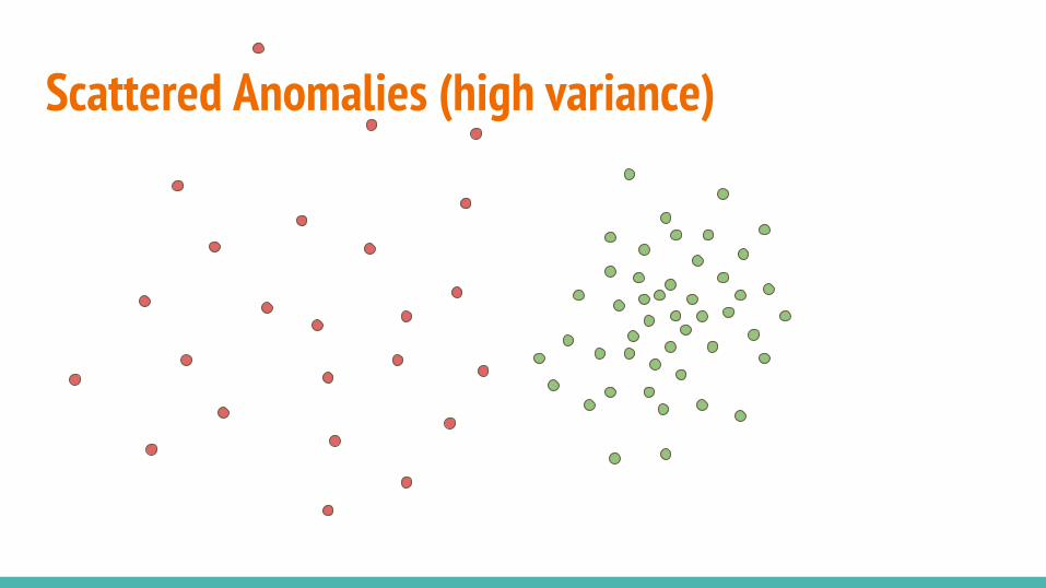
Scattered Anomalies (high variance)

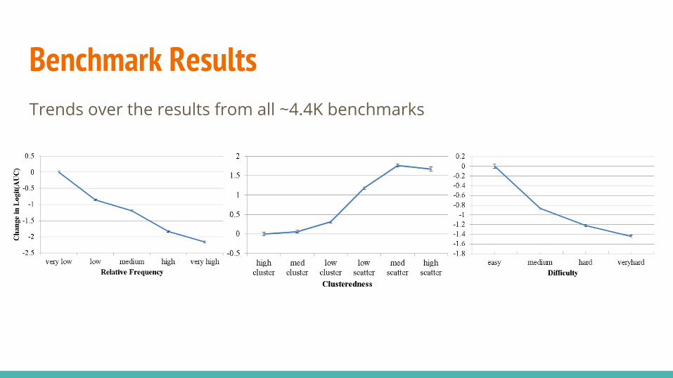
Benchmark ResultsTrends over the results from all ~4.4K benchmarks

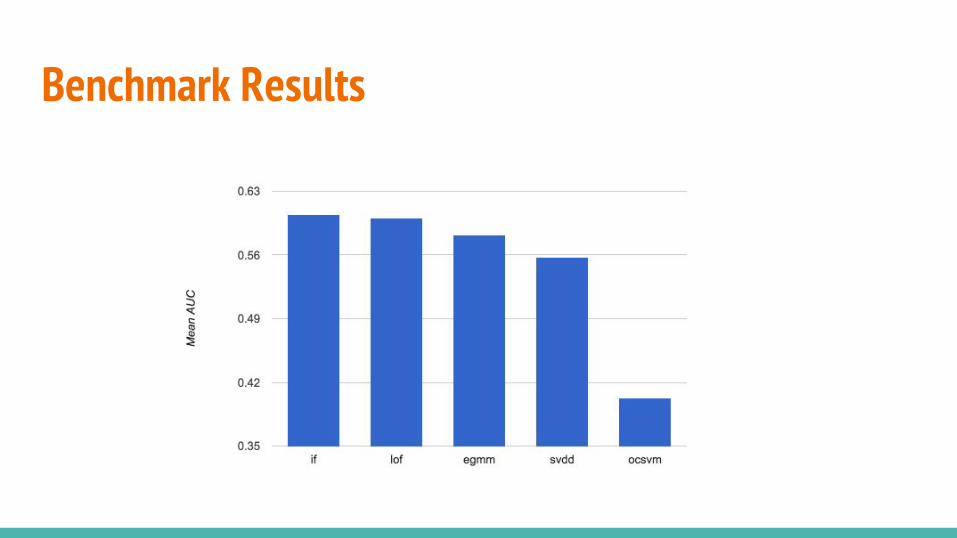
Benchmark Results

Isolation ForestsThe Good

● Very easy to construct (no distance function needed)● Gracefully handles missing values at scoring time● Can provide anomaly explanations ● Parameter free*

The Bad

● *Not really parameter free● Wide datasets will need more trees (how many?)● Needs extensions to handle discrete values and categorical data

Isolation ForestsThe Good

● Very easy to construct (no distance function needed)● Gracefully handles missing values at scoring time● Can provide anomaly explanations ● Parameter free*

The Bad

● *Not really parameter free● Wide datasets will need more trees (how many?)● Needs extensions to handle discrete values and categorical data

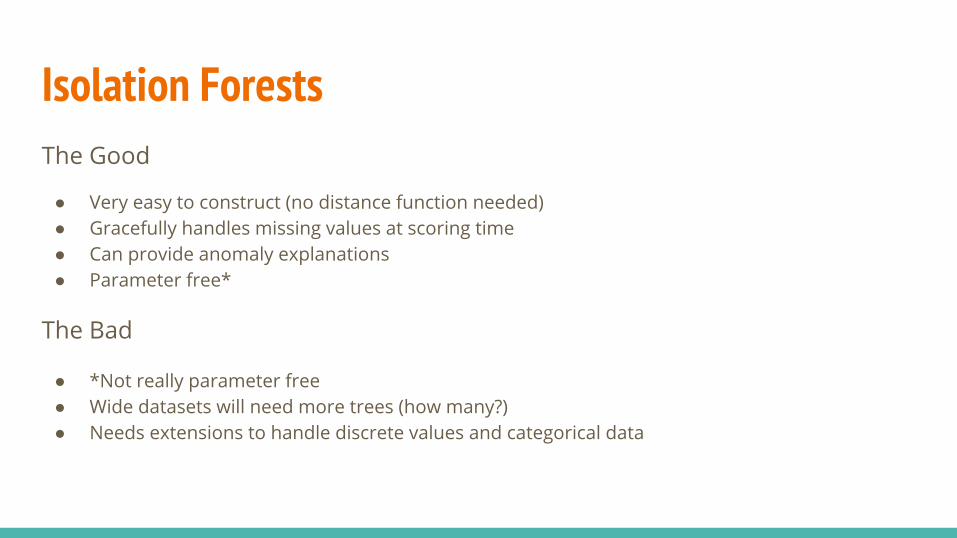
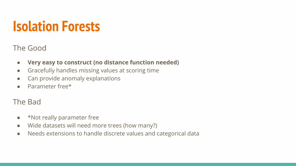
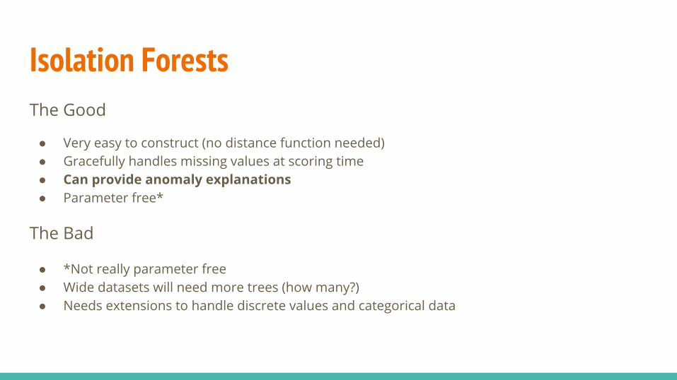
Isolation ForestsThe Good

● Very easy to construct (no distance function needed)● Gracefully handles missing values at scoring time● Can provide anomaly explanations ● Parameter free*

The Bad

● *Not really parameter free● Wide datasets will need more trees (how many?)● Needs extensions to handle discrete values and categorical data

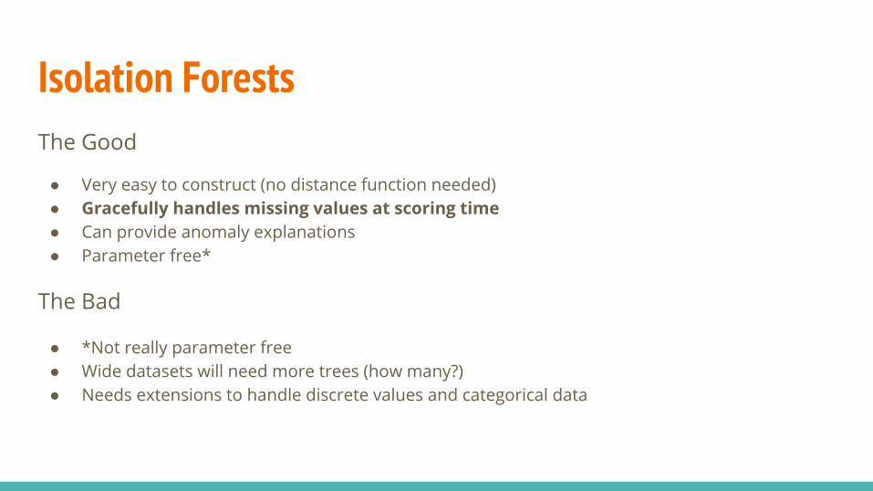
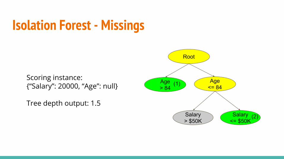
Isolation Forest - Missings

Age<= 84

Salary> $50K

Salary<= $50K

Scoring instance:{“Salary”: 20000, “Age”: null}

Root

Age> 84

Isolation Forest - Missings

Age<= 84

Salary> $50K

Salary<= $50K

Scoring instance:{“Salary”: 20000, “Age”: null}

Tree depth output: 1.5

Root

Age> 84

(1)

(2)

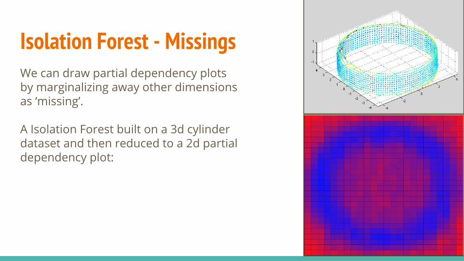
Isolation Forest - MissingsWe can draw partial dependency plots by marginalizing away other dimensions as ‘missing’.

A Isolation Forest built on a 3d cylinder dataset and then reduced to a 2d partial dependency plot:

Isolation ForestsThe Good

● Very easy to construct (no distance function needed)● Gracefully handles missing values at scoring time● Can provide anomaly explanations ● Parameter free*

The Bad

● *Not really parameter free● Wide datasets will need more trees (how many?)● Needs extensions to handle discrete values and categorical data

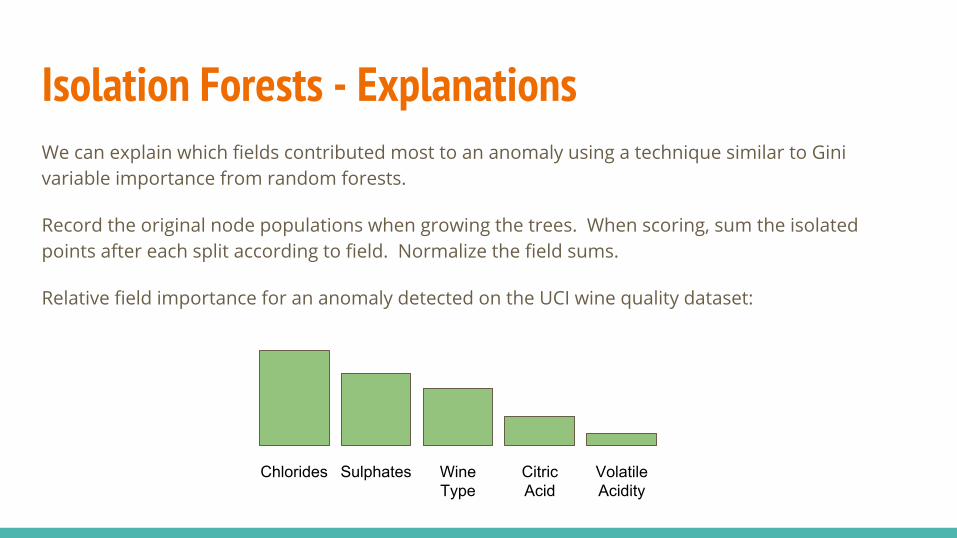
Isolation Forests - ExplanationsWe can explain which fields contributed most to an anomaly using a technique similar to Gini variable importance from random forests.

Record the original node populations when growing the trees. When scoring, sum the isolated points after each split according to field. Normalize the field sums.

Relative field importance for an anomaly detected on the UCI wine quality dataset:

Chlorides Sulphates WineType

CitricAcid

VolatileAcidity

Isolation ForestsThe Good

● Very easy to construct (no distance function needed)● Gracefully handles missing values at scoring time● Can provide anomaly explanations ● Parameter free*

The Bad

● *Not really parameter free● Wide datasets will need more trees (how many?)● Needs extensions to handle discrete values and categorical data

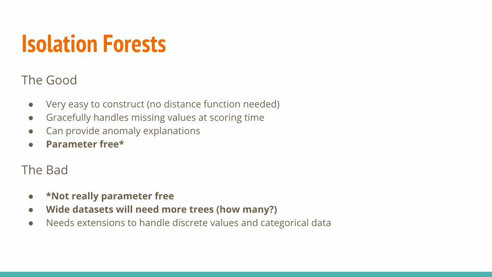
Isolation ForestsThe Good

● Very easy to construct (no distance function needed)● Gracefully handles missing values at scoring time● Can provide anomaly explanations ● Parameter free*

The Bad

● *Not really parameter free● Wide datasets will need more trees (how many?)● Needs extensions to handle discrete values and categorical data

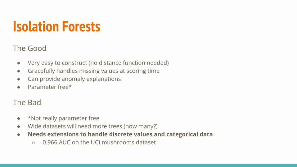
○ 0.966 AUC on the UCI mushrooms dataset