Heisman Trophy Voting: A Bayesian Analysis

Daniel Heard

Heisman Trophy Data

The data set consisted of season statistics from offensive finalistsfor the Heisman trophy, including passing yards, passingtouchdowns, rushing yards, rushing touchdowns, receiving yards,receiving touchdowns, and the number of wins the candidates teamhad in a given year. The data also included indicators as towhether the candidate’s team was undefeated, what conference thecandidates’ teams were members of and in which geographicalregion the candidates’ schools were located. Finally, the dataincluded the number of ballots received and total points thecandidates earned from voters from the 2000-2009 seasons.

Voting Process

In a given year, there are 870 media ballots, one fan ballot (basedon fans voting online for candidates) and each living recipient ofthe Heisman trophy is able to cast a ballot.Points are calculated as follows: on each ballot, the voter indicatestheir 1st, 2nd, and 3rd place candidates. Each first place vote isworth 3 points, second place votes are worth 2 points, and thirdplace votes are worth 1 point.In the event that every ballot is submitted, each candidate canreceive a maximum of 2778 points. However, it is unusual for morethan 97% of the ballots to be submitted.

Items of Interest

Items of interest regarding Heisman trophy voting include:

I Examining voting trends by position, conference, region andclass year of candidates

I Predicting voting for future candidates

Priors

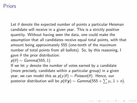
Let θ denote the expected number of points a particular Heismancandidate will receive in a given year. This is a strictly positivequantity. Without having seen the data, one could make theassumption that all candidates receive equal total points, with thatamount being approximately 555 (one-tenth of the maximumnumber of total points from all ballots). So, by this reasoning, Igave θ the prior distribution:p(θ) ∼ Gamma(555, 1)If we let y denote the number of votes earned by a candidate(more precisely, candidate within a particular group) in a givenyear, we can model this as p(y |θ) ∼ Poisson(θ). Hence, ourposterior distribution will be p(θ|y) ∼ Gamma(555 +

∑yi , 1 + n).

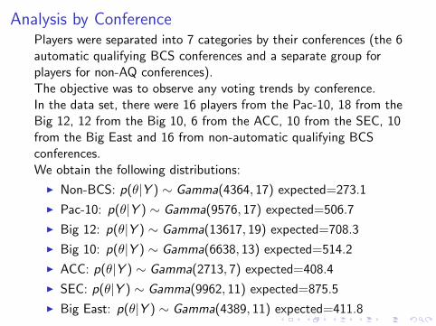
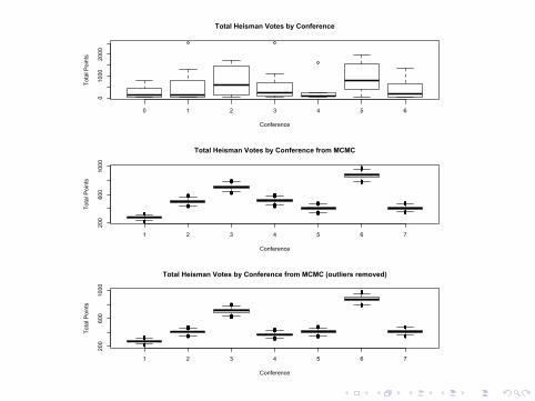
Analysis by ConferencePlayers were separated into 7 categories by their conferences (the 6automatic qualifying BCS conferences and a separate group forplayers for non-AQ conferences).The objective was to observe any voting trends by conference.In the data set, there were 16 players from the Pac-10, 18 from theBig 12, 12 from the Big 10, 6 from the ACC, 10 from the SEC, 10from the Big East and 16 from non-automatic qualifying BCSconferences.We obtain the following distributions:

I Non-BCS: p(θ|Y ) ∼ Gamma(4364, 17) expected=273.1

I Pac-10: p(θ|Y ) ∼ Gamma(9576, 17) expected=506.7

I Big 12: p(θ|Y ) ∼ Gamma(13617, 19) expected=708.3

I Big 10: p(θ|Y ) ∼ Gamma(6638, 13) expected=514.2

I ACC: p(θ|Y ) ∼ Gamma(2713, 7) expected=408.4

I SEC: p(θ|Y ) ∼ Gamma(9962, 11) expected=875.5

I Big East: p(θ|Y ) ∼ Gamma(4389, 11) expected=411.8

0 1 2 3 4 5 6

01000

2000

Total Heisman Votes by Conference

Conference

Tota

l Poi

nts

1 2 3 4 5 6 7

200

600

1000

Total Heisman Votes by Conference from MCMC

Conference

Tota

l Poi

nts

1 2 3 4 5 6 7

200

600

1000

Total Heisman Votes by Conference from MCMC (outliers removed)

Conference

Tota

l Poi

nts

After performing analysis with the two outliers removed, theaverage points for Pac-10 by over 100 and lowered the averagepoints for the Big 10 by nearly 150, resulting in the followingaverages:

I Non-BCS:273.1

I Pac-10:404.8

I Big 12:708.3

I Big 10:369.9

I ACC:408.4

I SEC:876.7

I Big East:411.8

Analysis by RegionHeisman trophy voting is broken up into 6 geographic regions: FarWest, Midwest, Southwest, South, Mid-Atlantic and Northeast.Players were separated into the geographic region in which theirschool is located.Of interest was to see if there is a difference in the average numberof votes a player in a particular region will receive.In the data set, there were 24 players from the Far West, 19 fromthe Midwest, 20 from the Southwest, 14 from the South, 12 fromthe Mid-Atlantic and 1 from the Northeast.So, we obtain the following distributions:

I Far West:p(θ|Y ) ∼ Gamma(11498, 25), expected=463.5

I Midwest: p(θ|Y ) ∼ Gamma(7648, 20), expected=390.7

I Southwest:p(θ|Y ) ∼ Gamma(16242, 21), exp[ected=763.6

I South: p(θ|Y ) ∼ Gamma(10912, 15), expected=716.6

I Mid-Atlantic: p(θ|Y ) ∼ Gamma(3786, 13), expected=309.9

I Northeast: p(θ|Y ) ∼ Gamma(618, 2), expected=391.0

1 2 3 4 5 6

01000

2000

Total Heisman Votes by Region

Region

Tota

l Poi

nts

1 2 3 4 5 6

300

500

700

Total Heisman Votes by Region from MCMC

Region

Tota

l Poi

nts

1 2 3 4 5 6

300

500

700

Total Heisman Votes by Region from MCMC (outliers removed)

Region

Tota

l Poi

nts

Removing outliers lowered the average points for Far West regionby just under 100 and lowered the average points for the Midwestregion by just under 100, resulting in the following averages:

I Far West:385.4

I Midwest:294.7

I Southwest:763.3

I South: 716.8

I Mid-Atlantic:310.2

I Northeast: 390.6

The Mid-Atlantic region is actually the lowest region by points.Among BCS conferences, it contains most of the schools in theACC and the Big East, the lowest point totaling among the 6automatic-qualifying conferences.

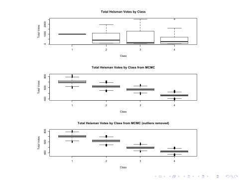
Analysis by Class

Player were grouped by class (Freshman, Sophomore, Junior,Senior)Of interest was to see if there is a difference in the average numberof votes players of a particular class will receive.In the data set, there was 1 freshman, 16 sophomores, 25 juniorsand 48 seniorsSo, we obtain the following distributions:

I Freshman:p(θ|Y ) ∼ Gamma(1552, 2), expected=701.9

I Sophomore: p(θ|Y ) ∼ Gamma(10608, 17), expected=620.4

I Junior: p(θ|Y ) ∼ Gamma(14779, 26), expected=568.1

I Senior: p(θ|Y ) ∼ Gamma(22655, 49), expected=463.8

1 2 3 4

01000

2000

Total Heisman Votes by Class

Class

Tota

l Vot

es

1 2 3 4

400

600

800

Total Heisman Votes by Class from MCMC

Class

Tota

l Vot

es

1 2 3 4

400

600

800

Total Heisman Votes by Class from MCMC (outliers removed)

Class

Tota

l Vot

es

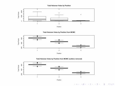
Analysis by Position

Player were grouped by offensive position (Quarterback, RunningBack, Wide Receiver).Of interest was to see if there is a difference in the average numberof votes different positions receive.In the data set, there were 52 quarterbacks, 29 running backs and9 wide receivers.We get the following distrubitions:

I Quarterback: p(θ|Y ) ∼ Gamma(32911, 53), expected=619.5

I Running Back: p(θ|Y ) ∼ Gamma(13775, 30), expected=462.1

I Wide Reciever:p(θ|Y ) ∼ Gamma(2353, 10), expected=264.1

1 2 3

01000

2000

Total Heisman Votes by Position

Position

Tota

l Poi

nts

1 2 3

200

400

600

Total Heisman Votes by Position from MCMC

Position

Tota

l Poi

nts

1 2 3

200

400

600

Total Heisman Votes by Position from MCMC (outliers removed)

Position

Tota

l Poi

nts

Removing outliers lowered the average points for quarterbacks byover 30 points and lowered the average points for running backs byover 60, resulting in the following averages:

I Quarterback: 582.6

I Running Back: 396.8

I Wide Receiver: 264.4

So, with outliers removed, the voting trend by position remains thesame.

Heisman Voting Linear Model

The 2010 Heisman trophy finalists were recently announced to be:

I LaMichael James, RB Oregon

I Andrew Luck, QB Stanford

I Kellen Moore, QB Boise State

I Cameron Newton, QB Auburn

I constructed a linear model to predict the number of points earnedby a Heisman finalist based on certain statistics. While thenumerical predictions of the model are not precise, the predictionsof relative number of votes is accurate. The formula for the modelis as follows:h.lm¡-lm(log(Votes) factor(Position) + factor(Conf) +sqrt(Wins) + PassTDs * factor(Position) + PassYds + Scrim *factor(Position) + Score * factor(Position) + factor(U), data = H)

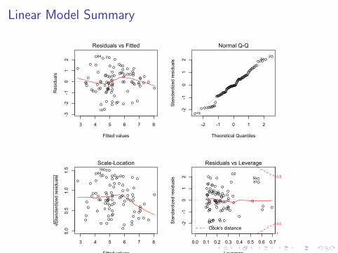
Linear Model Summary

3 4 5 6 7 8

-3-2

-10

12

Fitted values

Residuals

Residuals vs Fitted

18

84 2

-2 -1 0 1 2

-2-1

01

2

Theoretical Quantiles

Sta

ndar

dize

d re

sidu

als

Normal Q-Q

18

284

3 4 5 6 7 8

0.0

0.5

1.0

1.5

Fitted values

Standardized residuals

Scale-Location18 284

0.0 0.1 0.2 0.3 0.4 0.5 0.6 0.7

-2-1

01

2

Leverage

Sta

ndar

dize

d re

sidu

als

Cook's distance1

0.5

0.5

Residuals vs Leverage

5687

2

Placing a g-prior on the coefficients, I performed Monte Carlosampling with the prior sample size ν0 = 1, the prior varianceσ20 = 2.3171 found by ordinary least squares and the prior values ofthe coefficients obtained from the model matrix of the linearmodel. While the model was not precise in the predictions of thenumber of votes, it was accurate in the relative vote totals.

Based on the linear model, the predictions for this year’s Heismantrophy voting are:

I 1st place: Cameron Newton: 3338.2 (above possible pointtotal)

I 2nd place: LaMichael James: 313.6

I 3rd place: Andrew Luck: 101.3

I 4th place: Kellen Moore: 77.5

Limitations

There were a number of limitations to the data and the study. Theprimary limitation was the amount of dependence in the data.Because the number of votes and points a particular candidatereceives in a given year is not independent of the number of votesand points other candidates receive in a given year, I was limited inthe number of quantities I was able to compare.Another limitation was in the data available. One frequentlyreferenced quantity relating to Heisman trophy voting is thepercentage of their team’s total offense a particular candidateaccounted for. This is potentially an important figure, however itwas not available.

Findings

From the analysis I performed, I found a great deal of discrepancyof points earned based on the categories of region, class, position,and conference. There may be some truth to the ”West CoastBias” theory that West Coast teams receive fewer points from eastcoast voters based on the regional analysis.The trend in voting based on class is likely due to the fact that thelast three Heisman trophy winners have been sophomores.It appears that conference and region led to the largest disparity inthe average number of total points a candidate receives. Thedifference in votes by conference is most likely the result of voters’perceptions of certain conferences being ”stronger” than others,and thus favoring players from these stronger conferences.