Embed Size (px)
Citation preview

Backprop,Gradient Descent,
And Auto Differentiation
Sam Abrahams, Memdump LLC

https://goo.gl/tKOvr7
Link to these slides:

YO!I am Sam Abrahams
I am a data scientist and engineer.You can find me on GitHub @samjabrahams
Buy my book:TensorFlow for Machine Intelligence
1.Gradient Descent
Guess and Check for Adults
Gradient Descent Outline
▣ Problem: fit data▣ Basic OLS linear regression▣ Visualize error curve and regression line▣ Step by step through changes

Scatter Plot
Simple Start: Linear Regression

Ordinary Least Squares Linear Regression
Simple Start: Linear Regression

Simple Start: Linear Regression
▣ Want to find a model that can fit our data▣ Could do it algebraically…
▣ BUT that doesn’t generalize well
Simple Start: Linear Regression
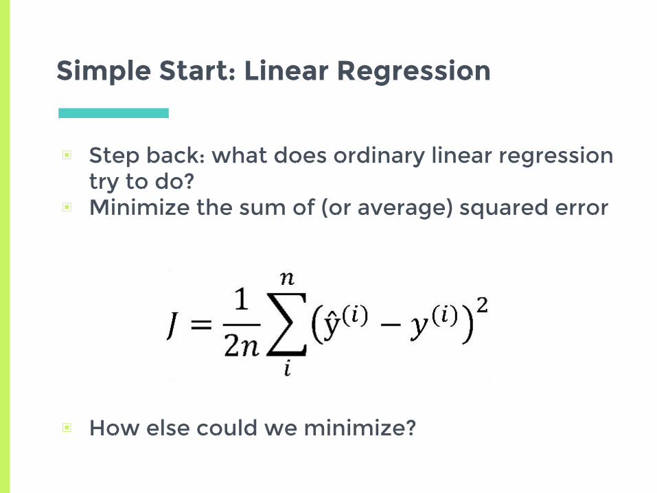
▣ Step back: what does ordinary linear regression try to do?
▣ Minimize the sum of (or average) squared error
▣ How else could we minimize?
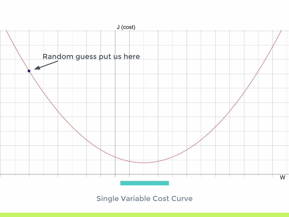
Gradient Descent
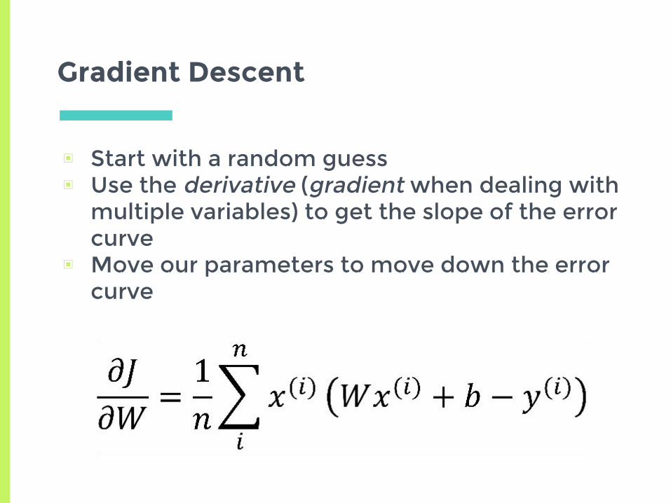
▣ Start with a random guess▣ Use the derivative (gradient when dealing with
multiple variables) to get the slope of the error curve
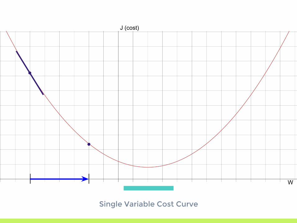
▣ Move our parameters to move down the error curve
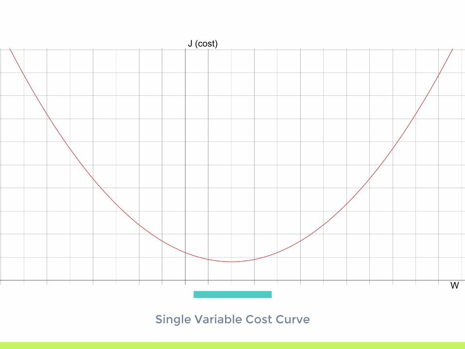
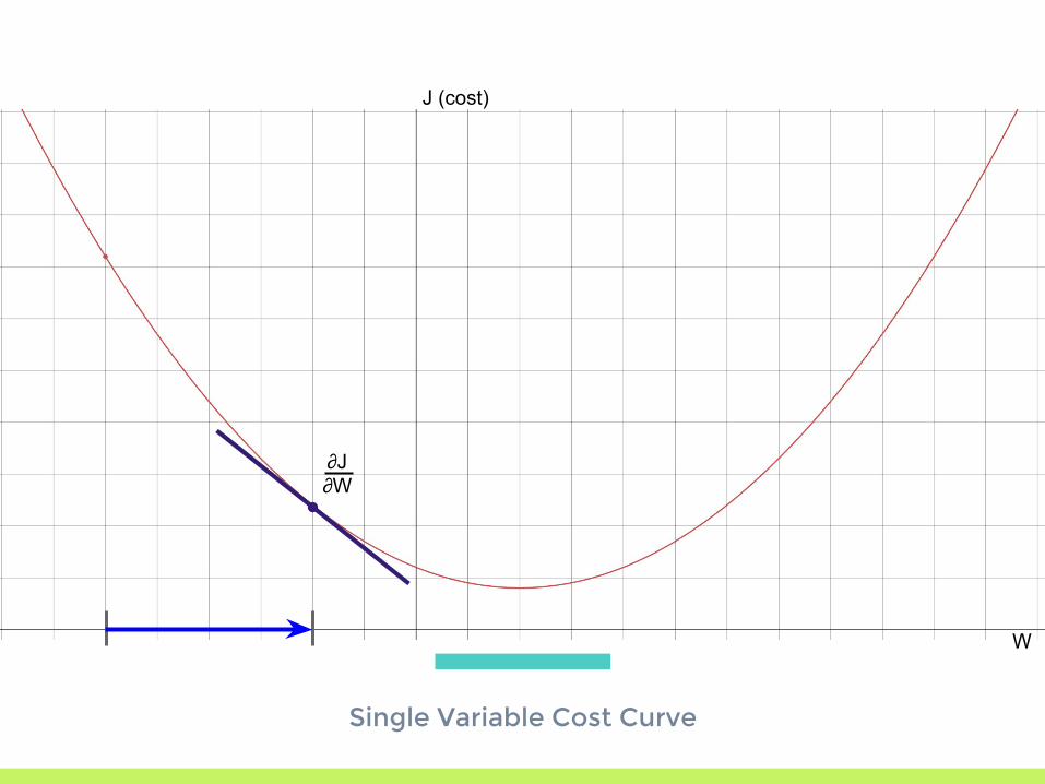
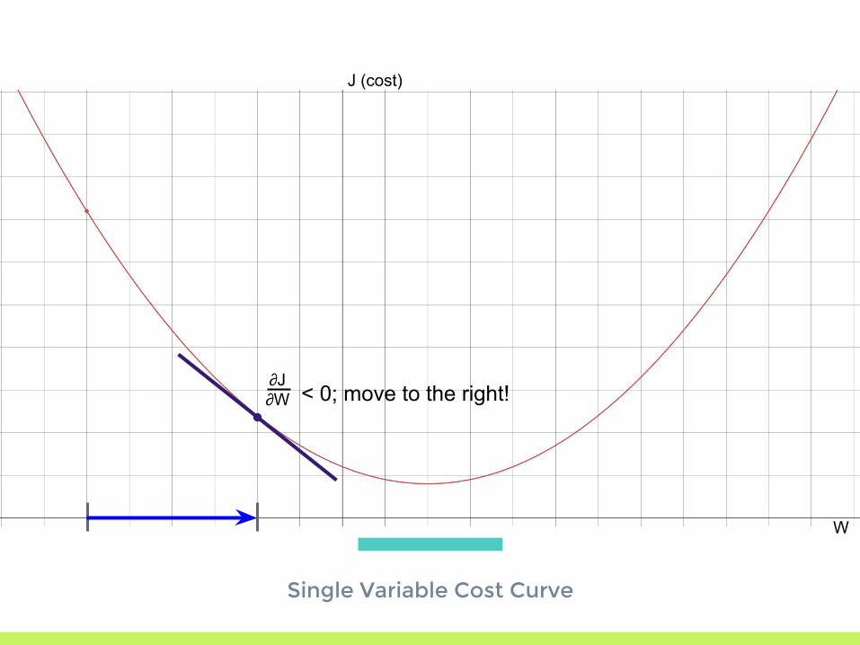
Single Variable Cost Curve
J (cost)
W
Single Variable Cost Curve
J (cost)
Random guess put us here
W
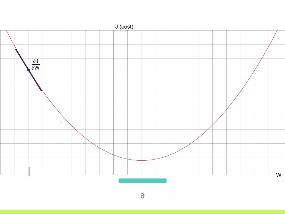
∂
W
J (cost)
∂J∂W

∂
W
J (cost)
∂J∂W < 0

∂
W
J (cost)
∂J∂W < 0; move to the right!
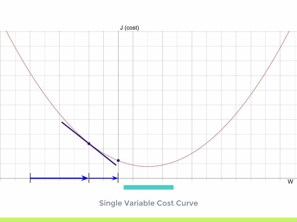
Single Variable Cost Curve
J (cost)
W
Single Variable Cost Curve
J (cost)
W
∂J∂W

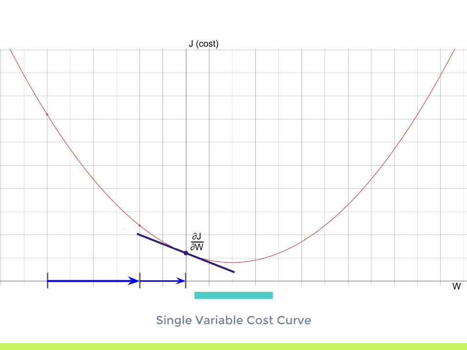
Single Variable Cost Curve
J (cost)
W
∂J∂W < 0
Single Variable Cost Curve
J (cost)
W
∂J∂W < 0; move to the right!
Single Variable Cost Curve
J (cost)
W
Single Variable Cost Curve
J (cost)
W
∂J∂W
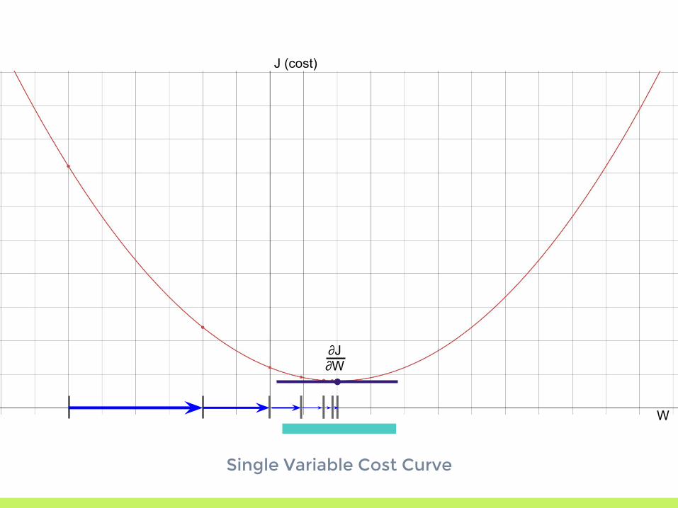
Single Variable Cost Curve
J (cost)
W
∂J∂W

Single Variable Cost Curve
J (cost)
∂J∂W
W

1.5Gradient
Descent VariantsIntelligent descent into madness
Gradient Descent Variants
▣ There are additional techniques that can help speed up (or otherwise improve) gradient descent
▣ The next slides describe some of these!▣ More details (and some awesome visuals)
here: article by Sebastian Ruder

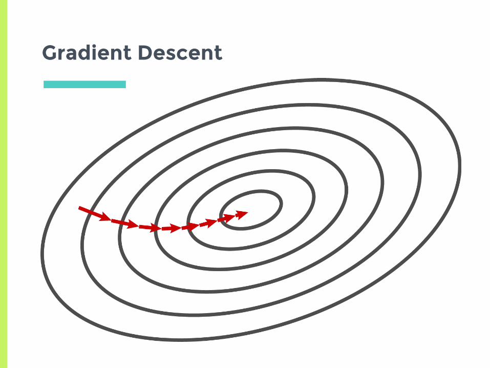
Gradient Descent
▣Get true gradient with respect to all examples▣One step = one epoch▣Slow and generally unfeasible for large training sets
Gradient Descent
Stochastic Gradient Descent
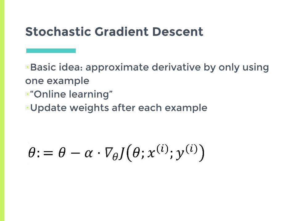
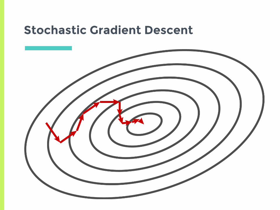
▣Basic idea: approximate derivative by only using one example▣“Online learning”▣Update weights after each example
Stochastic Gradient Descent
Mini-Batch Gradient Descent
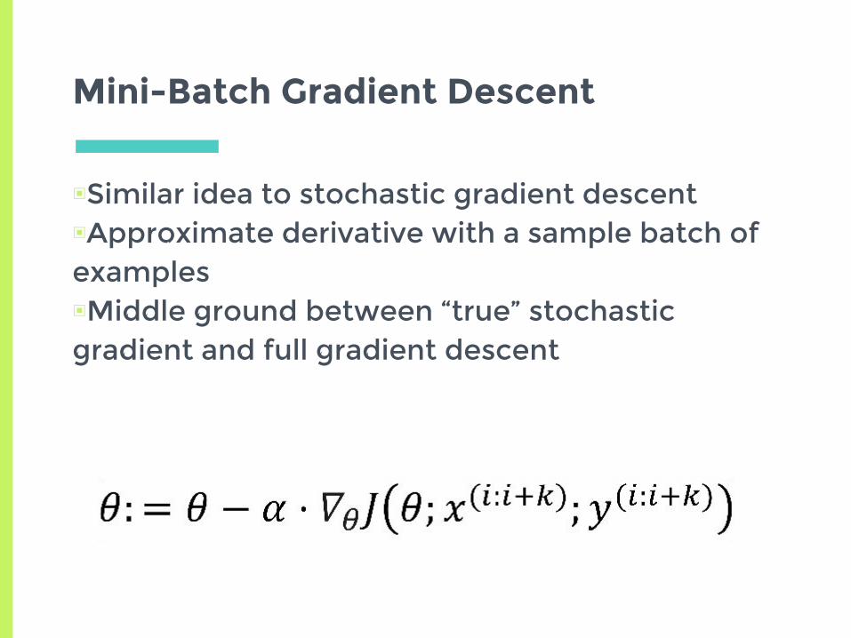
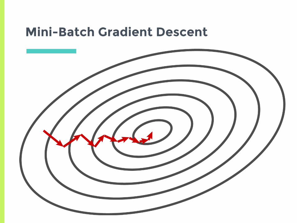
▣Similar idea to stochastic gradient descent▣Approximate derivative with a sample batch of examples▣Middle ground between “true” stochastic gradient and full gradient descent
Mini-Batch Gradient Descent
Momentum
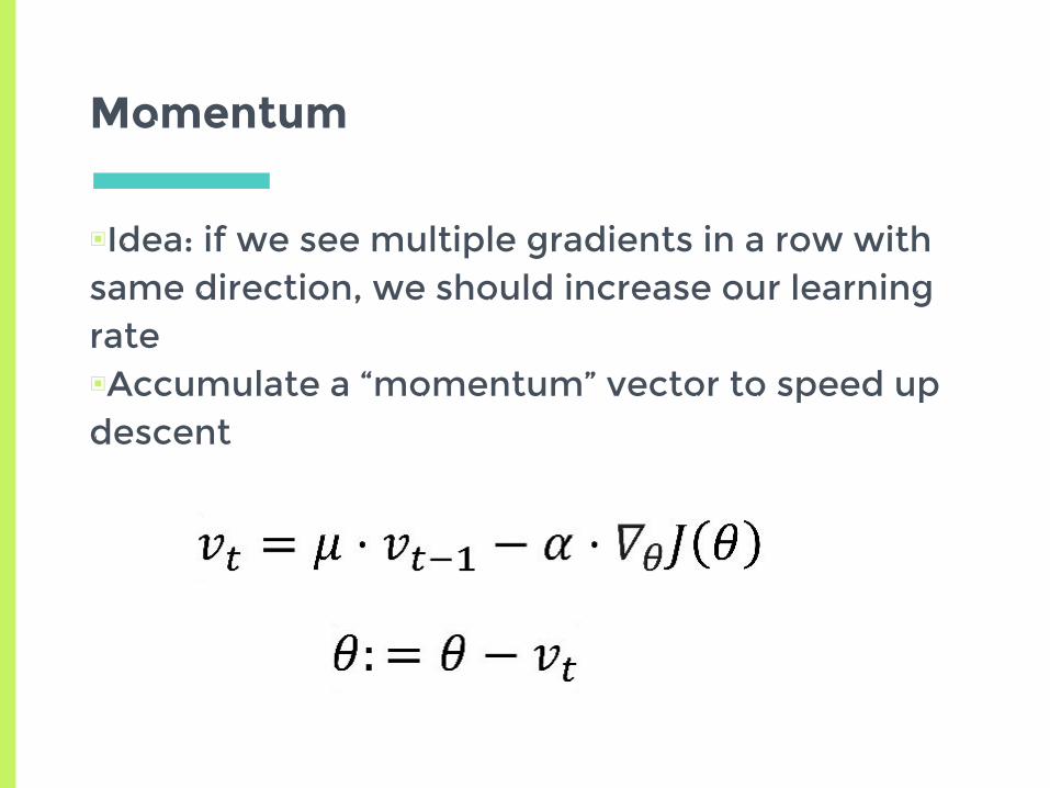
▣Idea: if we see multiple gradients in a row with same direction, we should increase our learning rate▣Accumulate a “momentum” vector to speed up descent
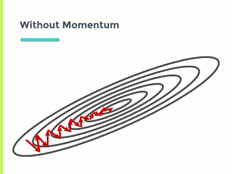
Without Momentum
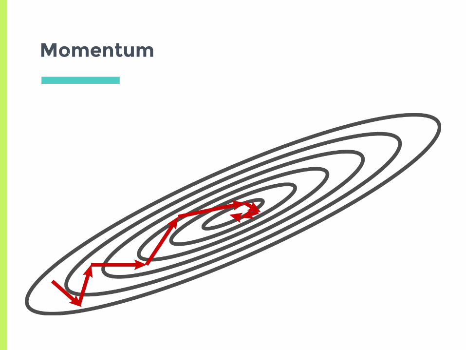
Momentum
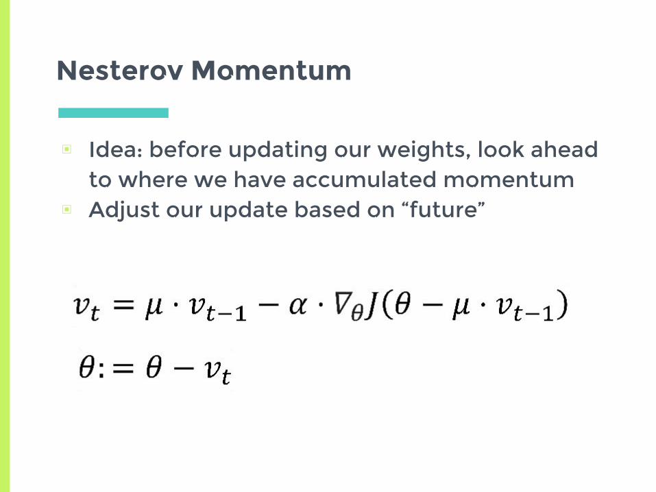
Nesterov Momentum
▣ Idea: before updating our weights, look ahead to where we have accumulated momentum
▣ Adjust our update based on “future”
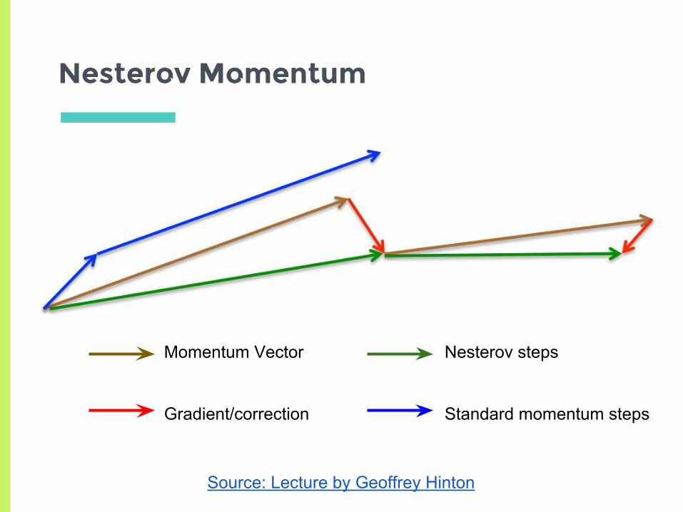
Nesterov Momentum
Source: Lecture by Geoffrey Hinton
Momentum Vector
Gradient/correction
Nesterov steps
Standard momentum steps
AdaGrad
▣ Idea: update individual weights differently depending on how frequently they change
▣ Keeps a running tally of previous updates for each weight, and divides new updates by a factor of the previous updates
▣ Downside: for long running training, eventually all gradients diminish
▣ Paper on jmlr.org
AdaDelta / RMSProp
▣ Two slightly different algorithms with same concept: only keep a window of the previous n gradients when scaling updates
▣ Seeks to reduce diminishing gradient problem with AdaGrad
▣ AdaDelta Paper on arxiv.org

Adam
▣ Adam expands on the concepts introduced with AdaDelta and RMSProp
▣ Uses both first order and second order moments, decayed over time
▣ Paper on arxiv.org

2.Forward & Back
PropagationThe Chain Rule got the last laugh, high-school-you

Beyond OLS Regression
▣ Can’t do everything with linear regression!▣ Nor polynomial…▣ Why can’t we let the computer figure out how
to model?

Neural Networks: Idea
▣ Chain together non-linear functions▣ Have lots of parameters that can be adjusted▣ These “weights” determine the model function
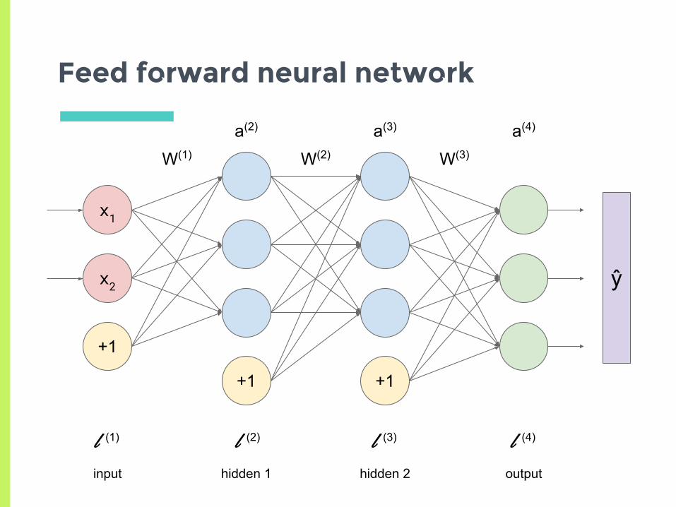
Feed forward neural network
+1 +1
x1
x2
+1
l (2) l (3) l (4)l (1)
input hidden 1 hidden 2 output
W(1) W(2) W(3)
a(2) a(3) a(4)
ŷ
σ
σ
σ
+1
σ
σ
σ
+1
SM
SM
SM
x1
x2
+1
W(1) W(2) W(3)
a(2) a(3) a(4)
ŷ
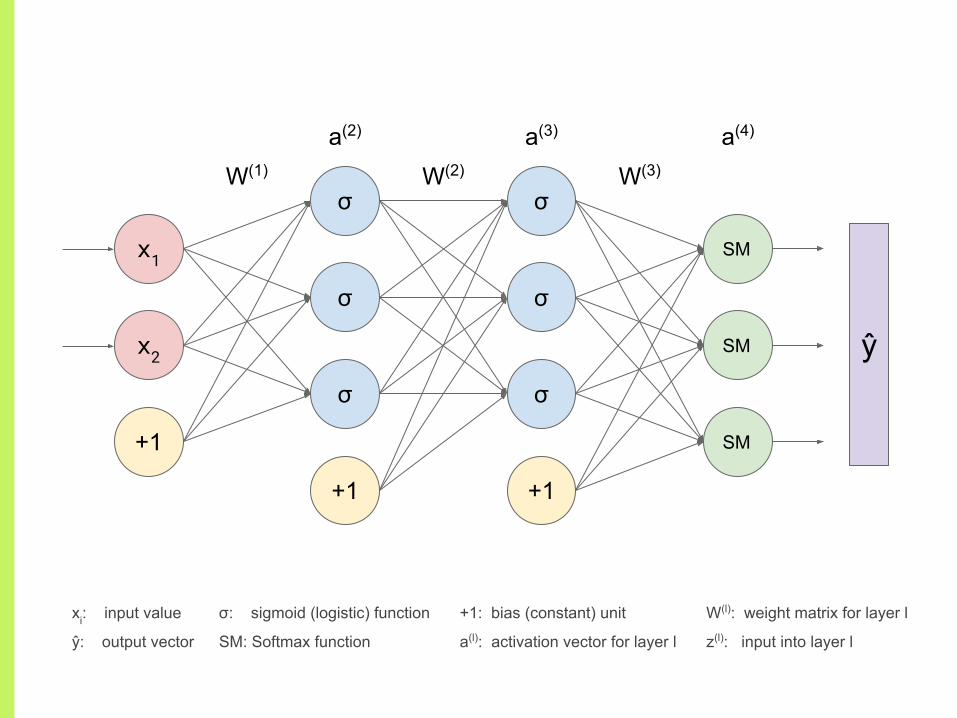
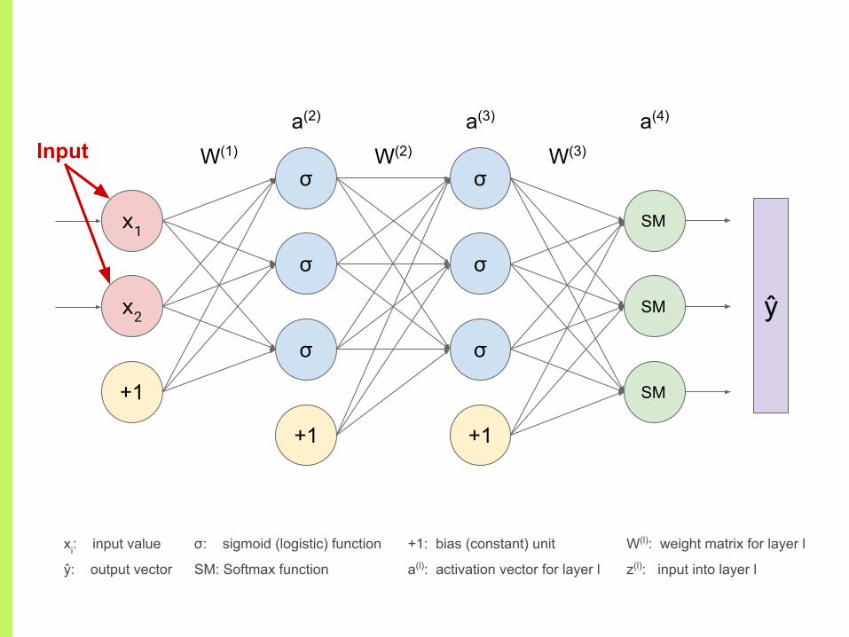
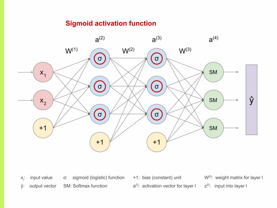
xi: input value
ŷ: output vector
+1: bias (constant) unit
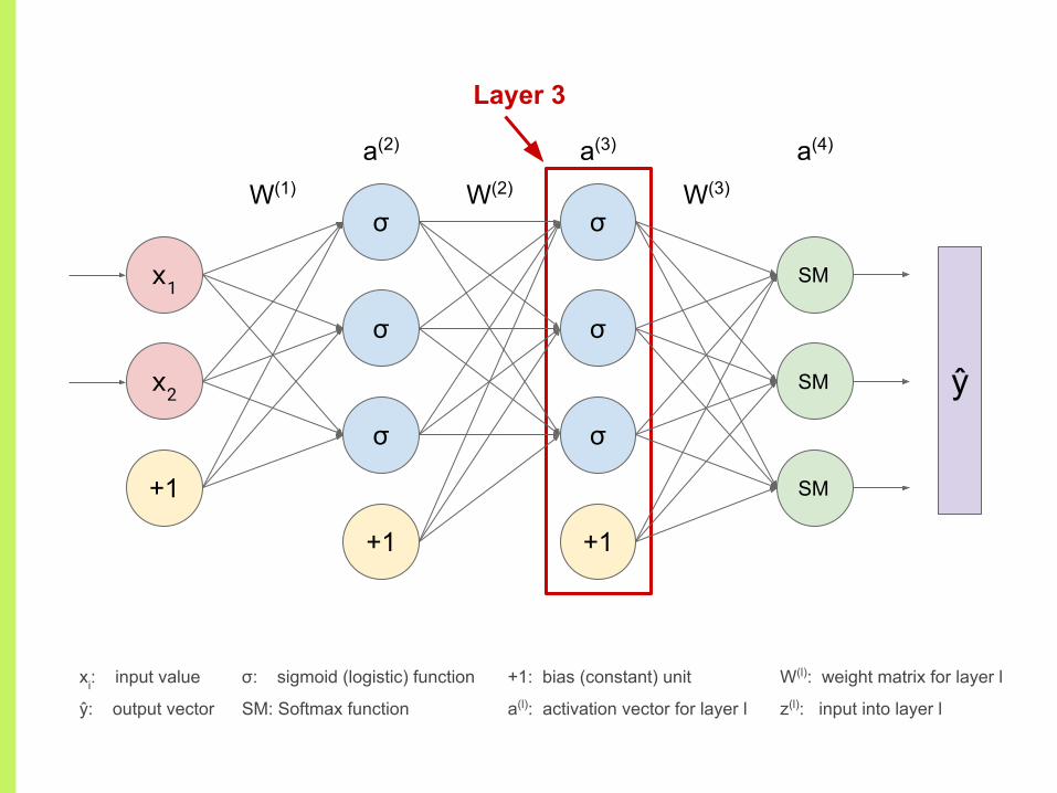
a(l): activation vector for layer l
W(l): weight matrix for layer l
z(l): input into layer l
σ: sigmoid (logistic) function
SM: Softmax function
σ
σ
σ
+1
σ
σ
σ
+1
x1
x2
+1
W(1) W(2) W(3)
a(2) a(3) a(4)
ŷ
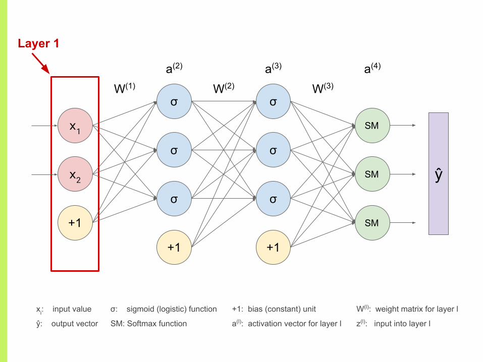
xi: input value
ŷ: output vector
+1: bias (constant) unit
a(l): activation vector for layer l
Layer 1
W(l): weight matrix for layer l
z(l): input into layer l
SM
SM
SM
σ: sigmoid (logistic) function
SM: Softmax function

σ
σ
σ
+1
σ
σ
σ
+1
x1
x2
+1
W(1) W(2) W(3)
a(2) a(3) a(4)
ŷ
xi: input value
ŷ: output vector
+1: bias (constant) unit
a(l): activation vector for layer l
Layer 2
W(l): weight matrix for layer l
z(l): input into layer l
SM
SM
SM
σ: sigmoid (logistic) function
SM: Softmax function
σ
σ
σ
+1
σ
σ
σ
+1
x1
x2
+1
W(1) W(2) W(3)
a(2) a(3) a(4)
ŷ
xi: input value
ŷ: output vector
+1: bias (constant) unit
a(l): activation vector for layer l
Layer 3
W(l): weight matrix for layer l
z(l): input into layer l
SM
SM
SM
σ: sigmoid (logistic) function
SM: Softmax function

σ
σ
σ
+1
σ
σ
σ
+1
x1
x2
+1
W(1) W(2) W(3)
a(2) a(3) a(4)
ŷ
xi: input value
ŷ: output vector
+1: bias (constant) unit
a(l): activation vector for layer l
Layer 4
W(l): weight matrix for layer l
z(l): input into layer l
SM
SM
SM
σ: sigmoid (logistic) function
SM: Softmax function

σ
σ
σ
+1
σ
σ
σ
+1
x1
x2
+1
W(1) W(2) W(3)
a(2) a(3) a(4)
ŷ
xi: input value
ŷ: output vector
+1: bias (constant) unit
a(l): activation vector for layer l
Biases (constant units)
W(l): weight matrix for layer l
z(l): input into layer l
SM
SM
SM
σ: sigmoid (logistic) function
SM: Softmax function
σ
σ
σ
+1
σ
σ
σ
+1
x1
x2
+1
W(1) W(2) W(3)
a(2) a(3) a(4)
ŷ
xi: input value
ŷ: output vector
+1: bias (constant) unit
a(l): activation vector for layer l
Input
W(l): weight matrix for layer l
z(l): input into layer l
SM
SM
SM
σ: sigmoid (logistic) function
SM: Softmax function
σ
σ
σ
+1
σ
σ
σ
+1
x1
x2
+1
W(1) W(2) W(3)
a(2) a(3) a(4)
ŷ
xi: input value
ŷ: output vector
+1: bias (constant) unit
a(l): activation vector for layer l
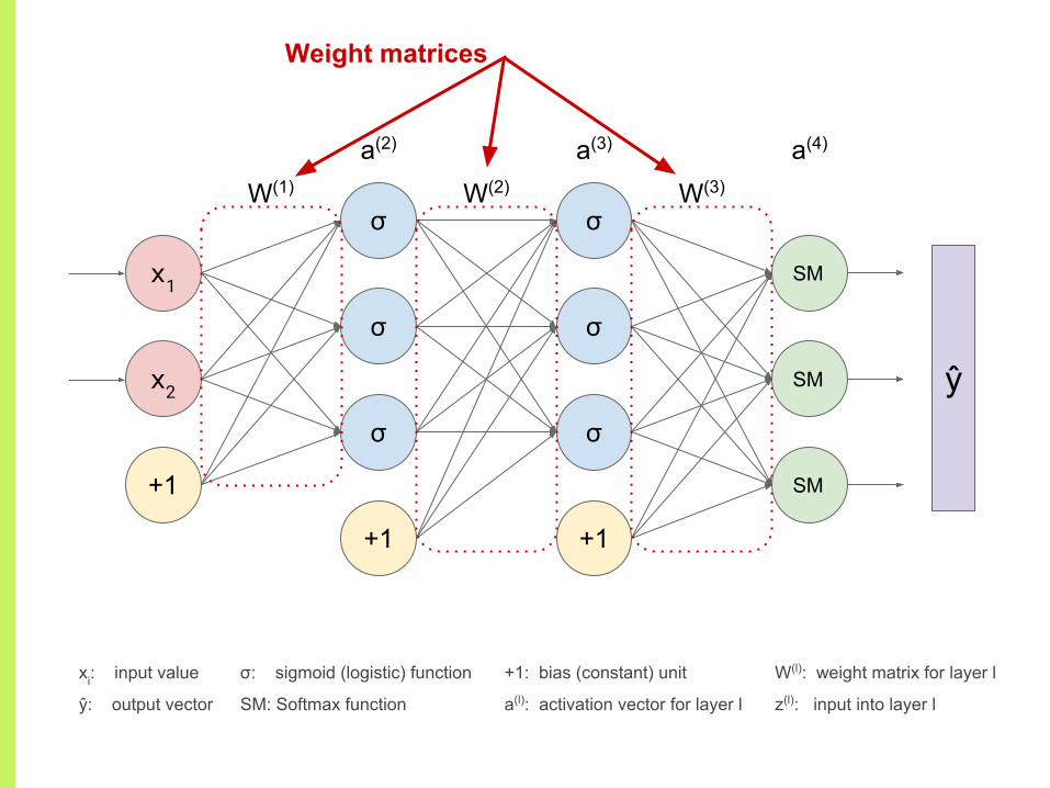
Weight matrices
W(l): weight matrix for layer l
z(l): input into layer l
SM
SM
SM
σ: sigmoid (logistic) function
SM: Softmax function
σ
σ
σ
+1
σ
σ
σ
+1
x1
x2
+1
W(1) W(2) W(3)
a(2) a(3) a(4)
ŷ
xi: input value
ŷ: output vector
+1: bias (constant) unit
a(l): activation vector for layer l
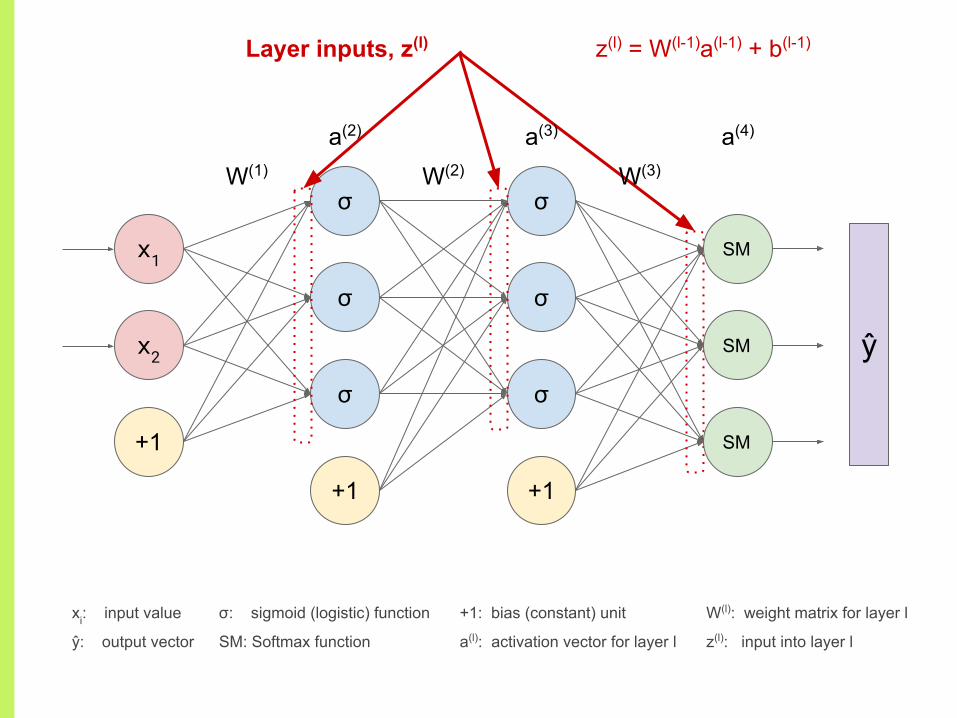
Layer inputs, z(l)
W(l): weight matrix for layer l
z(l): input into layer l
z(l) = W(l-1)a(l-1) + b(l-1)
SM
SM
SM
σ: sigmoid (logistic) function
SM: Softmax function

σ
σ
σ
+1
σ
σ
σ
+1
x1
x2
+1
W(1) W(2) W(3)
a(2) a(3) a(4)
ŷ
xi: input value
ŷ: output vector
+1: bias (constant) unit
a(l): activation vector for layer l
Activation vectors
W(l): weight matrix for layer l
z(l): input into layer l
SM
SM
SM
σ: sigmoid (logistic) function
SM: Softmax function
σ
σ
σ
+1
σ
σ
σ
+1
x1
x2
+1
W(1) W(2) W(3)
a(2) a(3) a(4)
ŷ
xi: input value
ŷ: output vector
+1: bias (constant) unit
a(l): activation vector for layer l
Sigmoid activation function
W(l): weight matrix for layer l
z(l): input into layer l
SM
SM
SM
σ: sigmoid (logistic) function
SM: Softmax function

SM
SM
SM
σ
σ
σ
+1
σ
σ
σ
+1
x1
x2
+1
W(1) W(2) W(3)
a(2) a(3) a(4)
ŷ
xi: input value
ŷ: output vector
+1: bias (constant) unit
a(l): activation vector for layer l
Softmax activation function
W(l): weight matrix for layer l
z(l): input into layer l
σ: sigmoid (logistic) function
SM: Softmax function

σ
σ
σ
+1
σ
σ
σ
+1
x1
x2
+1
W(1) W(2) W(3)
a(2) a(3) a(4)
ŷ
σ: sigmoid (logistic) function
SM: Softmax function
xi: input value
ŷ: output vector
+1: bias (constant) unit
a(l): activation vector for layer l
W(l): weight matrix for layer l
z(l): input into layer l
Output
SM
SM
SM
x1
x2
W(1) W(2) W(3)
a(2) a(3) a(4)
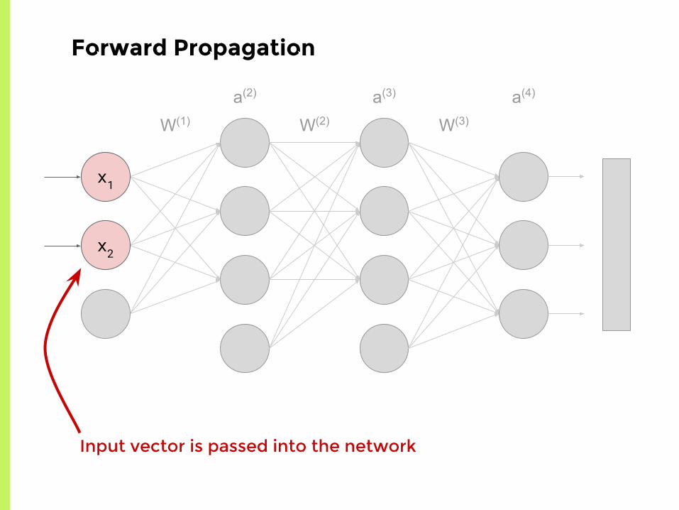
Forward Propagation
Input vector is passed into the network
x1
x2
+1
W(1)
a(2)
W(2) W(3)
a(3) a(4)
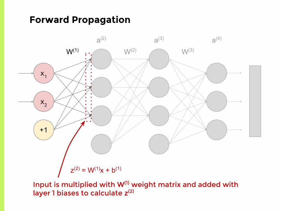
Forward Propagation
Input is multiplied with W(1) weight matrix and added with layer 1 biases to calculate z(2)
z(2) = W(1)x + b(1)

σ
σ
σ
x1
x2
+1
W(1)
a(2)
Forward Propagation
W(2) W(3)
a(3) a(4)
Activation value for the second layer is calculated by passing z(2) into some function. In this case, the sigmoid function.
a(2) = σ(z(2))
σ
σ
σ
+1
x1
x2
+1
W(1) W(2)
a(2)
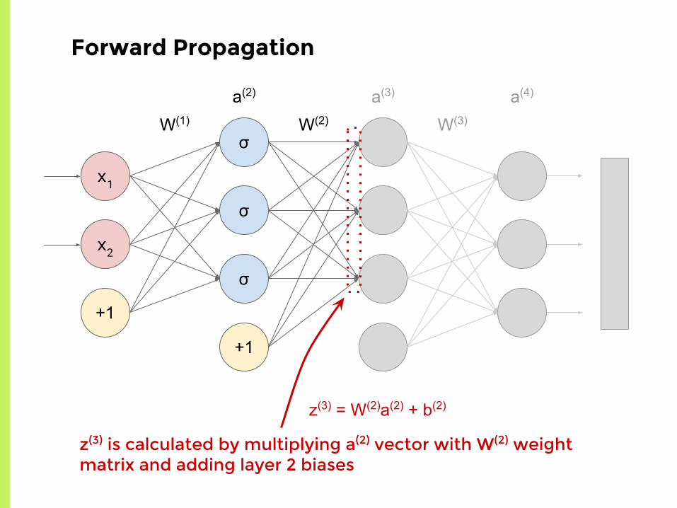
Forward Propagation
W(3)
a(3) a(4)
z(3) is calculated by multiplying a(2) vector with W(2) weight matrix and adding layer 2 biases
z(3) = W(2)a(2) + b(2)

σ
σ
σ
+1
σ
σ
σ
x1
x2
+1
W(1) W(2)
a(2) a(3)
Forward Propagation
Similar to previous layer, a(3) is calculated by passing z(3) into the sigmoid function
a(3) = σ(z(3))
W(3)

σ
σ
σ
+1
σ
σ
σ
+1
x1
x2
+1
W(1) W(2) W(3)
a(2) a(3)
Forward Propagation
z(4) is calculated by multiplying a(3) vector with W(3) weight matrix and adding layer 3 biases
z(4) = W(3)a(3) + b(3)
a(4)

σ
σ
σ
+1
σ
σ
σ
+1
x1
x2
+1
W(1) W(2) W(3)
a(2) a(3) a(4)
SM
SM
SM
Forward Propagation
For the final layer, we calculate a(4) by passing z(4) into the Softmax function
a(4) = SM(z(4))

σ
σ
σ
+1
σ
σ
σ
+1
x1
x2
+1
W(1) W(2) W(3)
a(2) a(3) a(4)
ŷ
SM
SM
SM
Forward Propagation
We then make our prediction based on the final layer’s output

Page of Math
z(2) = W(1)x + b(1)
z(3) = W(2)a(2) + b(2)
z(4) = W(3)a(3) + b(3)
a(2) = σ(z(2))
a(3) = σ(z(3))
a(4) = ŷ = SM(z(4))

Goal: Find which direction to shift weights
How: Find partial derivatives of the cost with respect to weight matrices
How (again): Chain rule the sh*t out of this mofo
DANGER:MATH

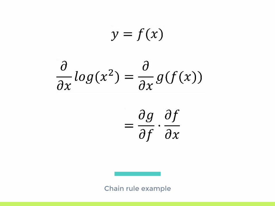
Chain Rule Reminder
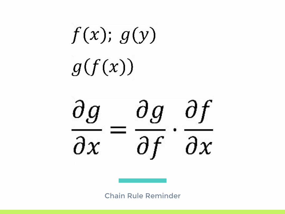
Chain Rule Reminder
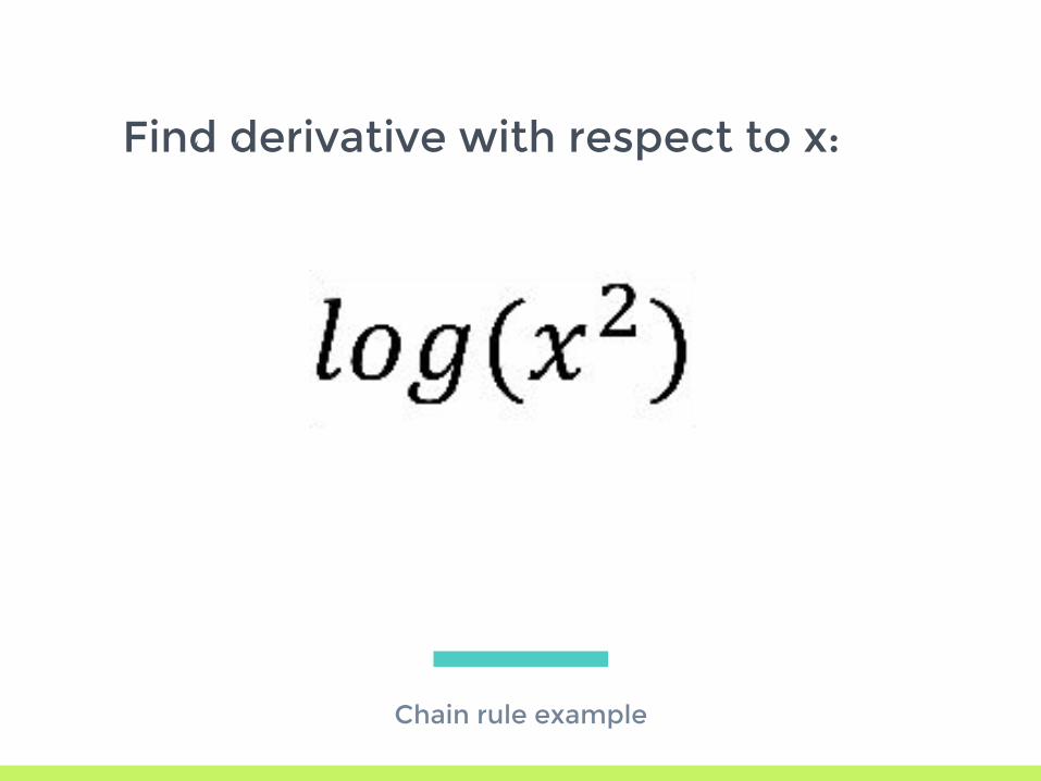
Chain rule example
Find derivative with respect to x:

Chain rule example
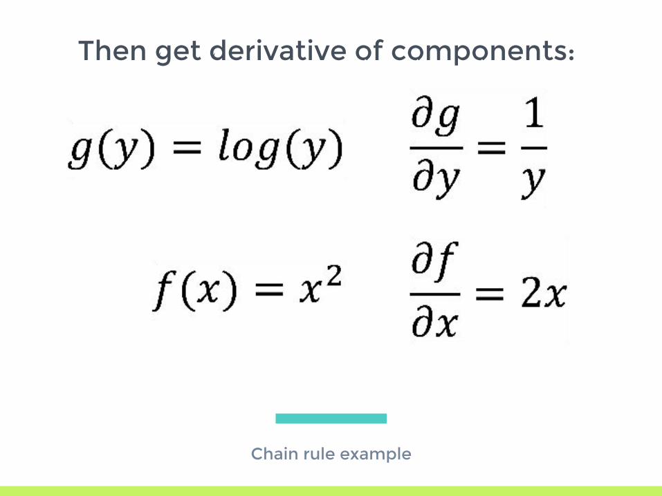
First split into two functions:
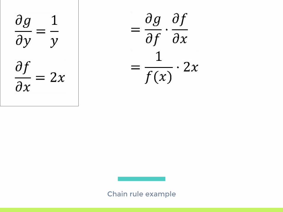
Chain rule example
Then get derivative of components:

Chain rule example

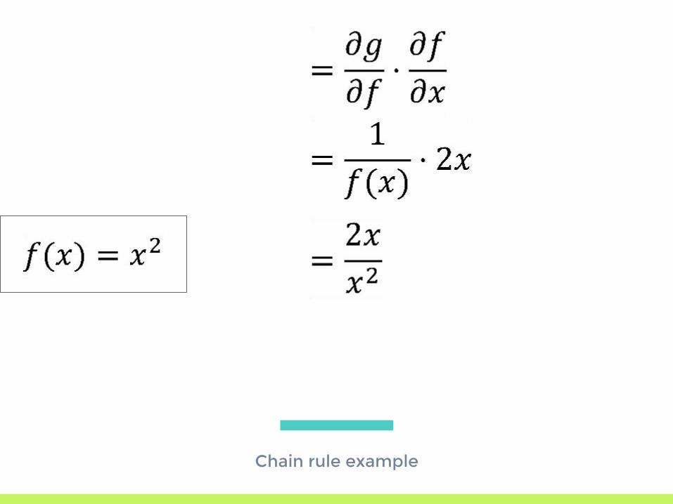
Chain rule example
Chain rule example

Chain rule example
Chain rule example
Chain rule example
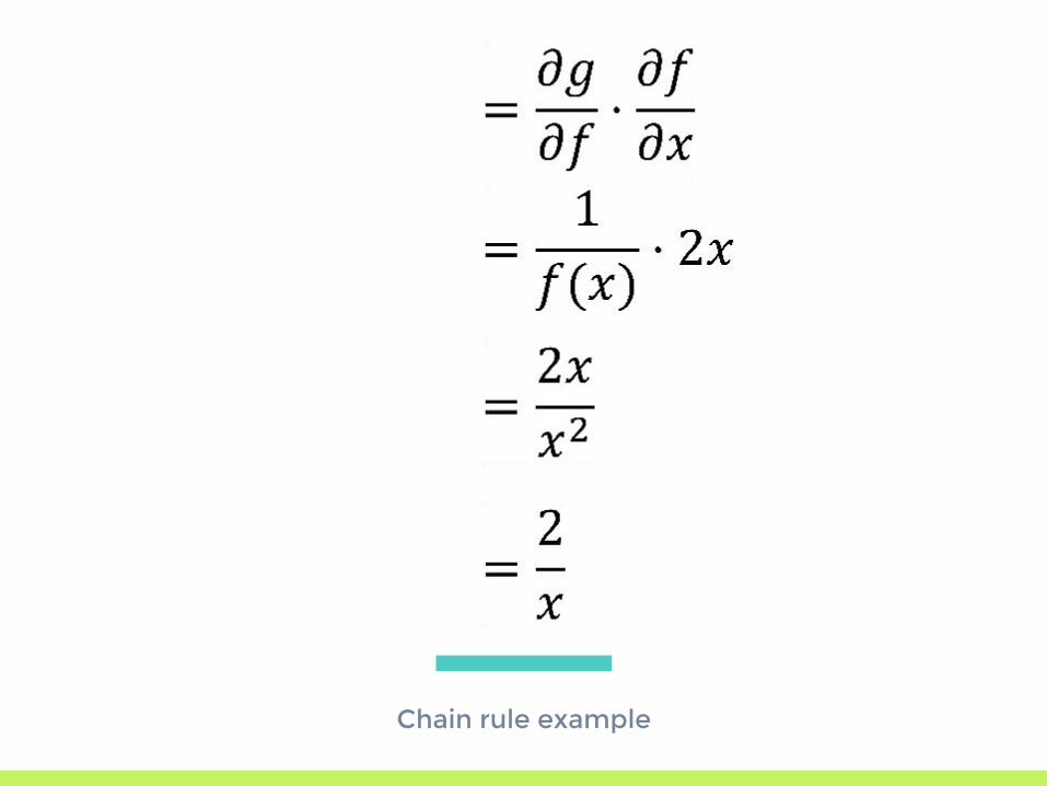
Chain rule example

DEEPER
DEEPER
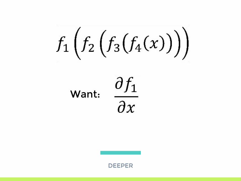
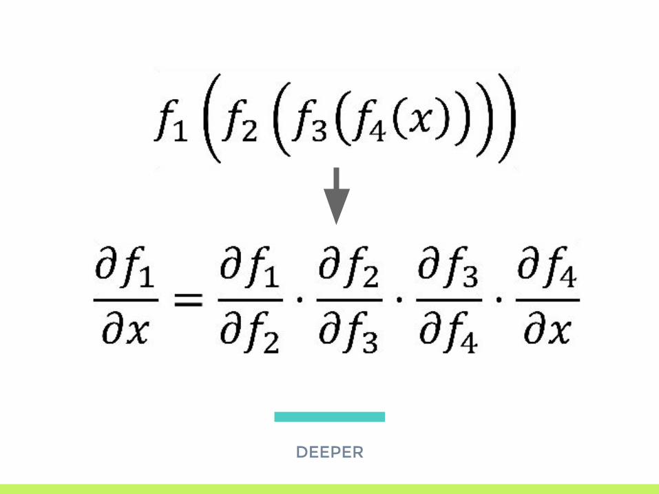
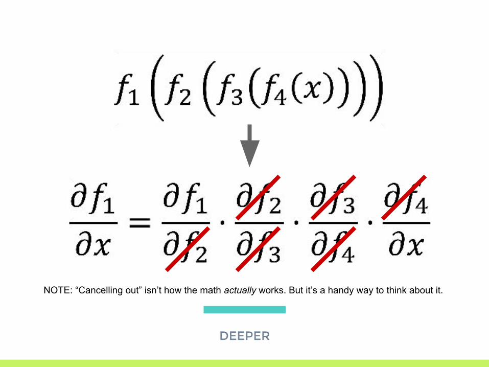
Want:
DEEPER
DEEPER
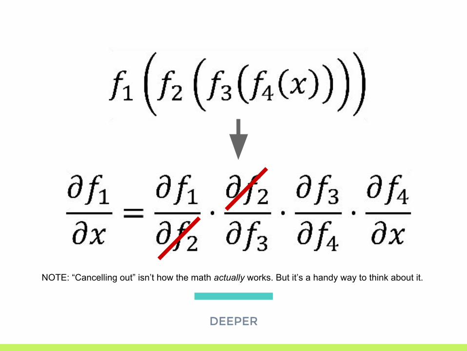
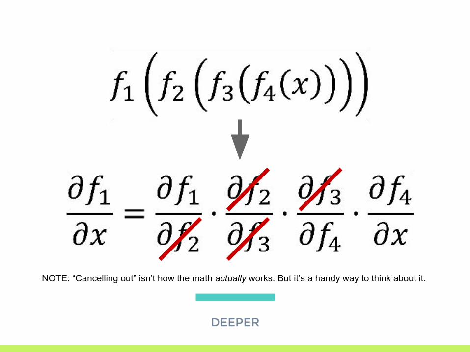
NOTE: “Cancelling out” isn’t how the math actually works. But it’s a handy way to think about it.
DEEPER
NOTE: “Cancelling out” isn’t how the math actually works. But it’s a handy way to think about it.
DEEPER
NOTE: “Cancelling out” isn’t how the math actually works. But it’s a handy way to think about it.

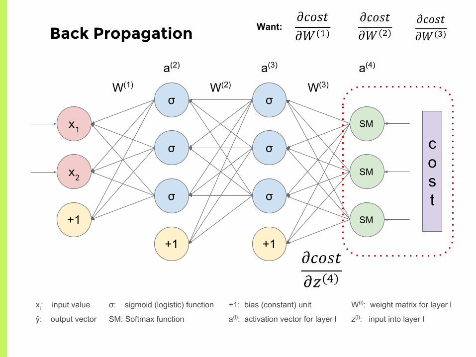
Back Prop
Back to backpropagation:
Want:

Return of Page of Math
z(2) = W(1)x + b(1)
z(3) = W(2)a(2) + b(2)
z(4) = W(3)a(3) + b(3)
a(2) = σ(z(2))
a(3) = σ(z(3))
a(4) = ŷ = SM(z(4))
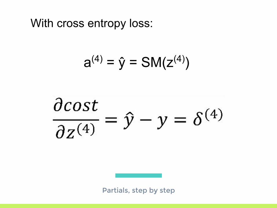
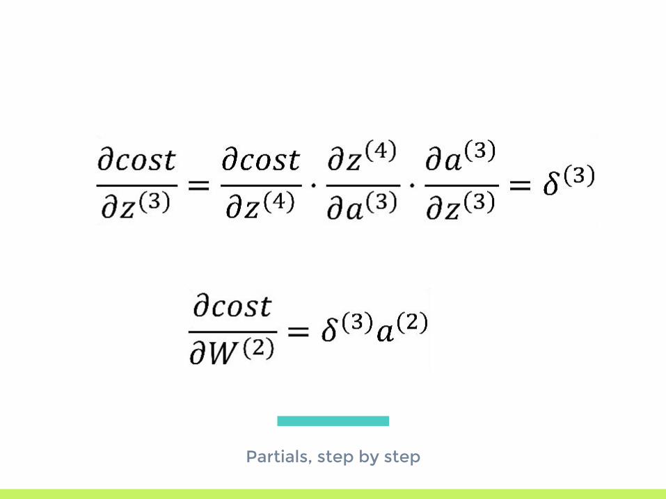
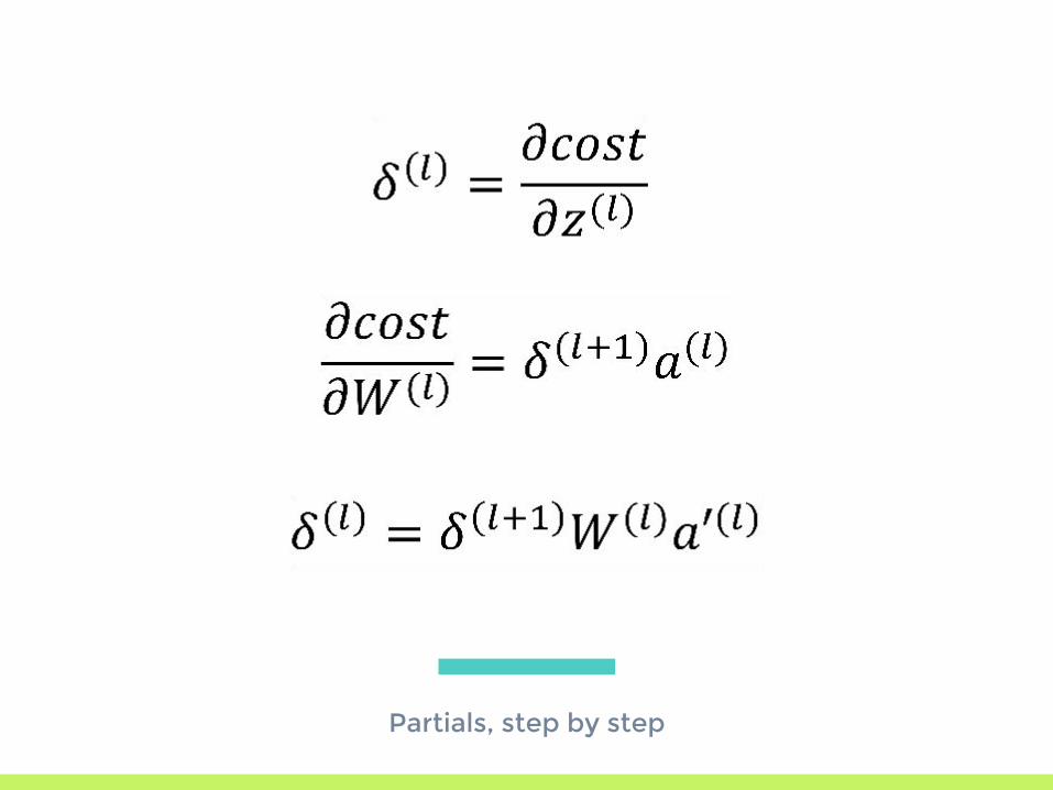
Partials, step by step
a(4) = ŷ = SM(z(4))
With cross entropy loss:
σ
σ
σ
+1
σ
σ
σ
+1
x1
x2
+1
W(1) W(2) W(3)
a(2) a(3) a(4)
cost
σ: sigmoid (logistic) function
SM: Softmax function
xi: input value
ŷ: output vector
+1: bias (constant) unit
a(l): activation vector for layer l
W(l): weight matrix for layer l
z(l): input into layer l
SM
SM
SM
Back Propagation Want:

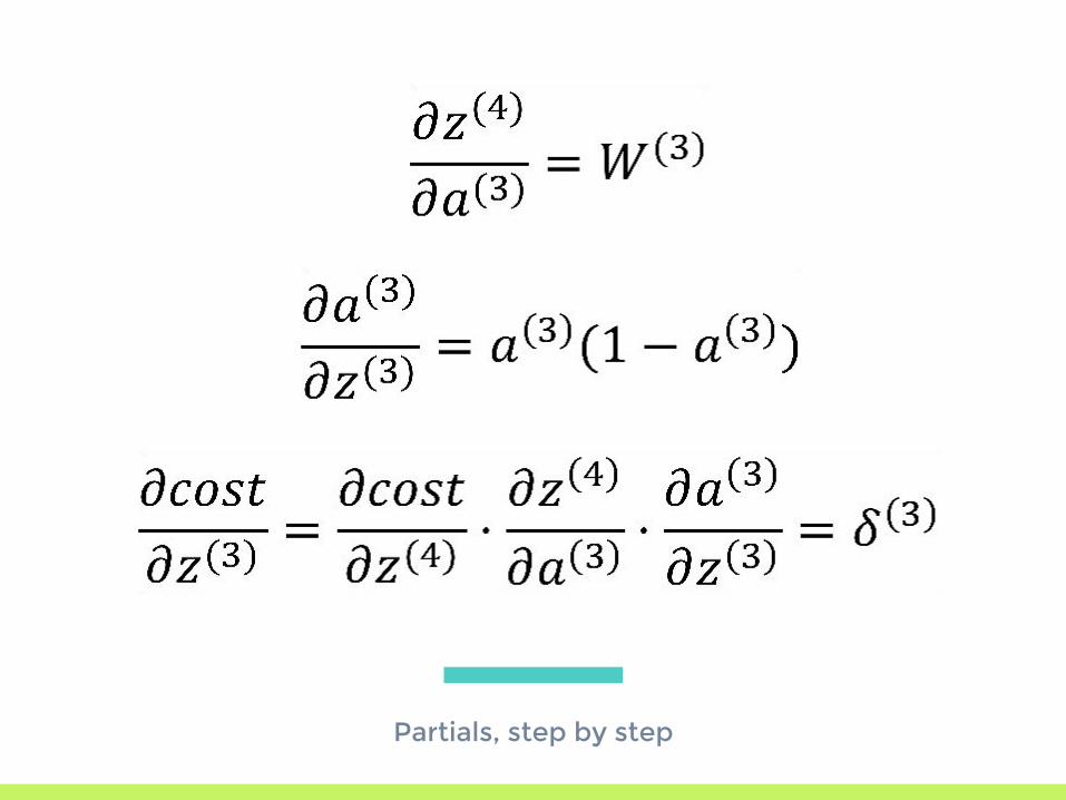
Partials, step by step

σ
σ
σ
+1
σ
σ
σ
+1
x1
x2
+1
W(1) W(2) W(3)
a(2) a(3) a(4)
cost
σ: sigmoid (logistic) function
SM: Softmax function
xi: input value
ŷ: output vector
+1: bias (constant) unit
a(l): activation vector for layer l
W(l): weight matrix for layer l
z(l): input into layer l
SM
SM
SM
Back Propagation Want:

σ
σ
σ
+1
σ
σ
σ
+1
x1
x2
+1
W(1) W(2) W(3)
a(2) a(3) a(4)
cost
σ: sigmoid (logistic) function
SM: Softmax function
xi: input value
ŷ: output vector
+1: bias (constant) unit
a(l): activation vector for layer l
W(l): weight matrix for layer l
z(l): input into layer l
SM
SM
SM
Back Propagation Want:

σ
σ
σ
+1
σ
σ
σ
+1
x1
x2
+1
W(1) W(2) W(3)
a(2) a(3) a(4)
cost
σ: sigmoid (logistic) function
SM: Softmax function
xi: input value
ŷ: output vector
+1: bias (constant) unit
a(l): activation vector for layer l
W(l): weight matrix for layer l
z(l): input into layer l
SM
SM
SM
Back Propagation Want:
Partials, step by step

As programmers...
How do we NOT do this ourselves?
We’re lazy by trade.
3.Automatic
DifferentiationBringing sexy lazy back
Why not hard code?
▣ Want to iterate fast!▣ Want flexibility▣ Want to reuse our code!
Auto-Differentiation: Idea
▣ Use functions that have easy-to-compute derivatives
▣ Compose these functions to create more complex super-model
▣ Use the chain rule to get partial derivatives of the model
What makes a “good” function?
▣ Obvious stuff: differentiable (continuously and smoothly!)
▣ Simple operations: add, subtract, multiply▣ Reuse previous computation

Nice functions: sigmoid
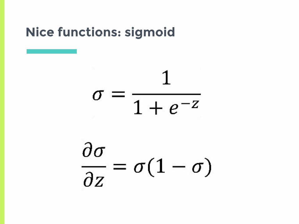
Nice functions: sigmoid

Nice functions: hyperbolic tangent
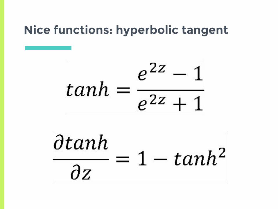
Nice functions: hyperbolic tangent

Nice functions: Rectified linear unit
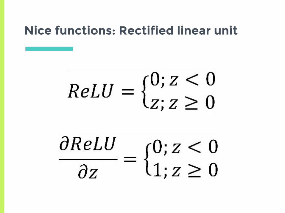
Nice functions: Rectified linear unit

Nice functions: Addition
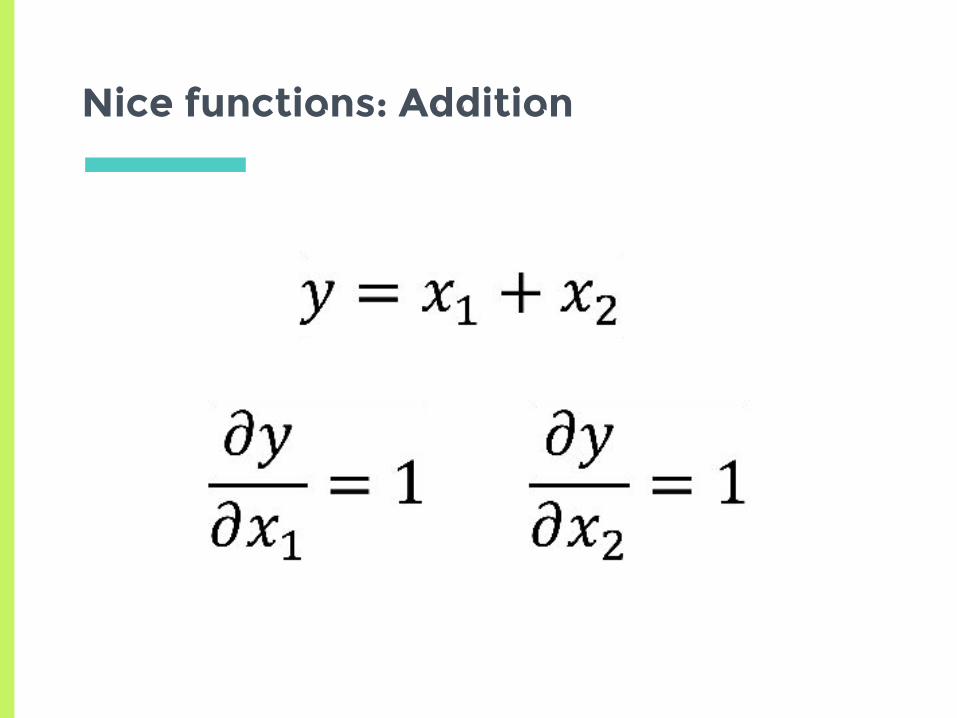
Nice functions: Addition
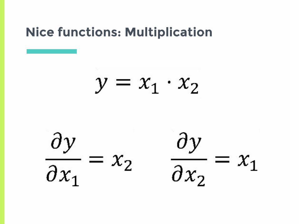
Nice functions: Multiplication

Good news:
Most of these use activation values! Can store in cache!

σ
σ
σ
+1
σ
σ
σ
+1
x1
x2
+1
W(1) W(2) W(3)
a(2) a(3) a(4)
ŷ
SM
SM
SM
Store activation values for backprop
σ
σ
σ
+1
σ
σ
σ
+1
x1
x2
+1
W(1) W(2) W(3)
a(2) a(3) a(4)
ŷ
SM
SM
SM
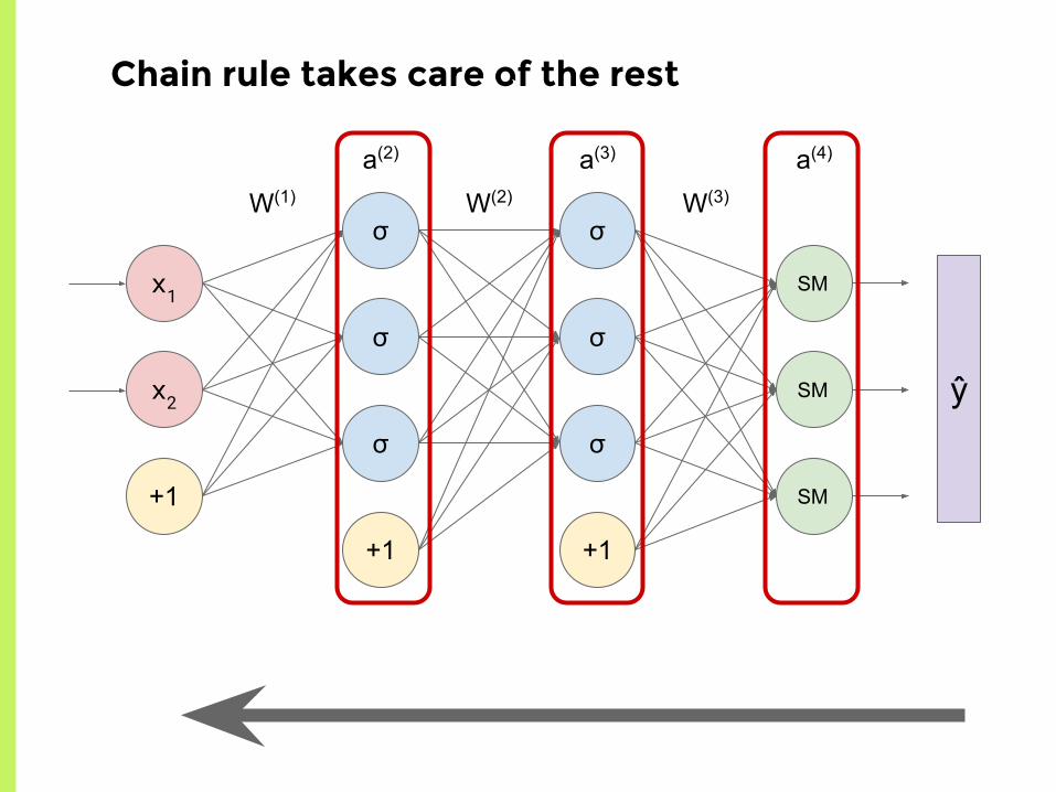
Chain rule takes care of the rest

It’s Over!Any questions?
Email: [email protected]: samjabrahamsTwitter: @sabraha
Presentation template by SlidesCarnival


Neural Network terms
▣ Neuron: a unit that transforms input via an activation function and outputs the result to other neurons and/or the final result
▣ Activation function: a(l), a transformation function, typically non-linear. Sigmoid, ReLU▣ Bias unit: a trainable scalar shift, typically applied to each non-output layer (think
y-intercept term in the linear function)▣ Layer: a grouping of “neurons” and biases that (in general) take in values from the same
previous neurons and pass values forwards to the same targets▣ Hidden layer: A layer that is neither the input layer nor the output layer▣ Input layer: ▣ Output layer
Terminology used
▣ Learning rate▣ Parameters▣ Training step▣ Training example▣ Epoch vs training time▣