Mastering the Game of Go with Deep Neural Networks andTree SearchDavid Silver1*, Aja Huang1*, Chris J. Maddison1, Arthur Guez1, Laurent Sifre1, George van denDriessche1, Julian Schrittwieser1, Ioannis Antonoglou1, Veda Panneershelvam1, Marc Lanctot1,Sander Dieleman1, Dominik Grewe1, John Nham2, Nal Kalchbrenner1, Ilya Sutskever2, TimothyLillicrap1, Madeleine Leach1, Koray Kavukcuoglu1, Thore Graepel1, Demis Hassabis1.

1 Google DeepMind, 5 New Street Square, London EC4A 3TW.2 Google, 1600 Amphitheatre Parkway, Mountain View CA 94043.

*These authors contributed equally to this work.

Correspondence should be addressed to either David Silver (davidsilver@google.com) or DemisHassabis (demishassabis@google.com).

The game of Go has long been viewed as the most challenging of classic games for ar-

tificial intelligence due to its enormous search space and the difficulty of evaluating board

positions and moves. We introduce a new approach to computer Go that uses value networks

to evaluate board positions and policy networks to select moves. These deep neural networks

are trained by a novel combination of supervised learning from human expert games, and

reinforcement learning from games of self-play. Without any lookahead search, the neural

networks play Go at the level of state-of-the-art Monte-Carlo tree search programs that sim-

ulate thousands of random games of self-play. We also introduce a new search algorithm

that combines Monte-Carlo simulation with value and policy networks. Using this search al-

gorithm, our program AlphaGo achieved a 99.8% winning rate against other Go programs,

and defeated the European Go champion by 5 games to 0. This is the first time that a com-

puter program has defeated a human professional player in the full-sized game of Go, a feat

previously thought to be at least a decade away.

All games of perfect information have an optimal value function, v∗(s), which determines

the outcome of the game, from every board position or state s, under perfect play by all players.

These games may be solved by recursively computing the optimal value function in a search tree

containing approximately bd possible sequences of moves, where b is the game’s breadth (number

1

of legal moves per position) and d is its depth (game length). In large games, such as chess

(b ≈ 35, d ≈ 80) 1 and especially Go (b ≈ 250, d ≈ 150) 1, exhaustive search is infeasible 2, 3,

but the effective search space can be reduced by two general principles. First, the depth of the

search may be reduced by position evaluation: truncating the search tree at state s and replacing

the subtree below s by an approximate value function v(s) ≈ v∗(s) that predicts the outcome from

state s. This approach has led to super-human performance in chess 4, checkers 5 and othello 6, but

it was believed to be intractable in Go due to the complexity of the game 7. Second, the breadth of

the search may be reduced by sampling actions from a policy p(a|s) that is a probability distribution

over possible moves a in position s. For example, Monte-Carlo rollouts 8 search to maximum depth

without branching at all, by sampling long sequences of actions for both players from a policy p.

Averaging over such rollouts can provide an effective position evaluation, achieving super-human

performance in backgammon 8 and Scrabble 9, and weak amateur level play in Go 10.

Monte-Carlo tree search (MCTS) 11, 12 uses Monte-Carlo rollouts to estimate the value of

each state in a search tree. As more simulations are executed, the search tree grows larger and the

relevant values become more accurate. The policy used to select actions during search is also im-

proved over time, by selecting children with higher values. Asymptotically, this policy converges

to optimal play, and the evaluations converge to the optimal value function 12. The strongest current

Go programs are based on MCTS, enhanced by policies that are trained to predict human expert

moves 13. These policies are used to narrow the search to a beam of high probability actions, and

to sample actions during rollouts. This approach has achieved strong amateur play 13–15. How-

ever, prior work has been limited to shallow policies 13–15 or value functions 16 based on a linear

combination of input features.

Recently, deep convolutional neural networks have achieved unprecedented performance

in visual domains: for example image classification 17, face recognition 18, and playing Atari

games 19. They use many layers of neurons, each arranged in overlapping tiles, to construct in-

creasingly abstract, localised representations of an image 20. We employ a similar architecture for

the game of Go. We pass in the board position as a 19 × 19 image and use convolutional layers

2

to construct a representation of the position. We use these neural networks to reduce the effective

depth and breadth of the search tree: evaluating positions using a value network, and sampling

actions using a policy network.

We train the neural networks using a pipeline consisting of several stages of machine learning

(Figure 1). We begin by training a supervised learning (SL) policy network, pσ, directly from

expert human moves. This provides fast, efficient learning updates with immediate feedback and

high quality gradients. Similar to prior work 13, 15, we also train a fast policy pπ that can rapidly

sample actions during rollouts. Next, we train a reinforcement learning (RL) policy network, pρ,

that improves the SL policy network by optimising the final outcome of games of self-play. This

adjusts the policy towards the correct goal of winning games, rather than maximizing predictive

accuracy. Finally, we train a value network vθ that predicts the winner of games played by the

RL policy network against itself. Our program AlphaGo efficiently combines the policy and value

networks with MCTS.

1 Supervised Learning of Policy Networks

For the first stage of the training pipeline, we build on prior work on predicting expert moves

in the game of Go using supervised learning13, 21–24. The SL policy network pσ(a|s) alternates

between convolutional layers with weights σ, and rectifier non-linearities. A final softmax layer

outputs a probability distribution over all legal moves a. The input s to the policy network is

a simple representation of the board state (see Extended Data Table 2). The policy network is

trained on randomly sampled state-action pairs (s, a), using stochastic gradient ascent to maximize

the likelihood of the human move a selected in state s,

∆σ ∝ ∂log pσ(a|s)∂σ

. (1)

We trained a 13 layer policy network, which we call the SL policy network, from 30 million

positions from the KGS Go Server. The network predicted expert moves with an accuracy of

3

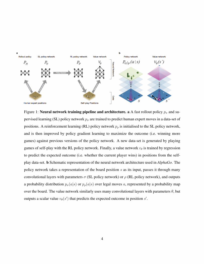
Figure 1: Neural network training pipeline and architecture. a A fast rollout policy pπ and su-

pervised learning (SL) policy network pσ are trained to predict human expert moves in a data-set of

positions. A reinforcement learning (RL) policy network pρ is initialised to the SL policy network,

and is then improved by policy gradient learning to maximize the outcome (i.e. winning more

games) against previous versions of the policy network. A new data-set is generated by playing

games of self-play with the RL policy network. Finally, a value network vθ is trained by regression

to predict the expected outcome (i.e. whether the current player wins) in positions from the self-

play data-set. b Schematic representation of the neural network architecture used in AlphaGo. The

policy network takes a representation of the board position s as its input, passes it through many

convolutional layers with parameters σ (SL policy network) or ρ (RL policy network), and outputs

a probability distribution pσ(a|s) or pρ(a|s) over legal moves a, represented by a probability map

over the board. The value network similarly uses many convolutional layers with parameters θ, but

outputs a scalar value vθ(s′) that predicts the expected outcome in position s′.

4

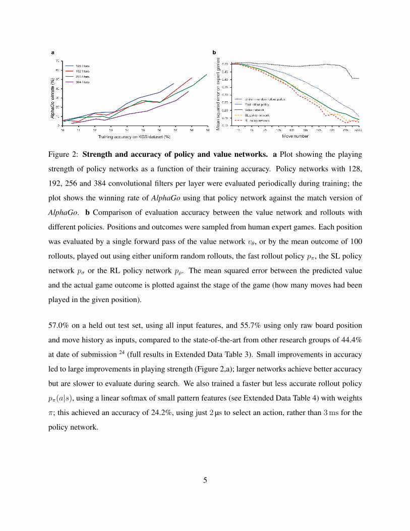
Figure 2: Strength and accuracy of policy and value networks. a Plot showing the playing

strength of policy networks as a function of their training accuracy. Policy networks with 128,

192, 256 and 384 convolutional filters per layer were evaluated periodically during training; the

plot shows the winning rate of AlphaGo using that policy network against the match version of

AlphaGo. b Comparison of evaluation accuracy between the value network and rollouts with

different policies. Positions and outcomes were sampled from human expert games. Each position

was evaluated by a single forward pass of the value network vθ, or by the mean outcome of 100

rollouts, played out using either uniform random rollouts, the fast rollout policy pπ, the SL policy

network pσ or the RL policy network pρ. The mean squared error between the predicted value

and the actual game outcome is plotted against the stage of the game (how many moves had been

played in the given position).

57.0% on a held out test set, using all input features, and 55.7% using only raw board position

and move history as inputs, compared to the state-of-the-art from other research groups of 44.4%

at date of submission 24 (full results in Extended Data Table 3). Small improvements in accuracy

led to large improvements in playing strength (Figure 2,a); larger networks achieve better accuracy

but are slower to evaluate during search. We also trained a faster but less accurate rollout policy

pπ(a|s), using a linear softmax of small pattern features (see Extended Data Table 4) with weights

π; this achieved an accuracy of 24.2%, using just 2 µs to select an action, rather than 3 ms for the

policy network.

5

2 Reinforcement Learning of Policy Networks

The second stage of the training pipeline aims at improving the policy network by policy gradient

reinforcement learning (RL) 25, 26. The RL policy network pρ is identical in structure to the SL

policy network, and its weights ρ are initialised to the same values, ρ = σ. We play games

between the current policy network pρ and a randomly selected previous iteration of the policy

network. Randomising from a pool of opponents stabilises training by preventing overfitting to the

current policy. We use a reward function r(s) that is zero for all non-terminal time-steps t < T .

The outcome zt = ±r(sT ) is the terminal reward at the end of the game from the perspective of the

current player at time-step t: +1 for winning and −1 for losing. Weights are then updated at each

time-step t by stochastic gradient ascent in the direction that maximizes expected outcome 25,

∆ρ ∝ ∂log pρ(at|st)∂ρ

zt . (2)

We evaluated the performance of the RL policy network in game play, sampling each move

at ∼ pρ(·|st) from its output probability distribution over actions. When played head-to-head,

the RL policy network won more than 80% of games against the SL policy network. We also

tested against the strongest open-source Go program, Pachi 14, a sophisticated Monte-Carlo search

program, ranked at 2 amateur dan on KGS, that executes 100,000 simulations per move. Using no

search at all, the RL policy network won 85% of games against Pachi. In comparison, the previous

state-of-the-art, based only on supervised learning of convolutional networks, won 11% of games

against Pachi 23 and 12% against a slightly weaker program Fuego 24.

3 Reinforcement Learning of Value Networks

The final stage of the training pipeline focuses on position evaluation, estimating a value function

vp(s) that predicts the outcome from position s of games played by using policy p for both players27–29,

vp(s) = E [zt | st = s, at...T ∼ p] . (3)

6

Ideally, we would like to know the optimal value function under perfect play v∗(s); in

practice, we instead estimate the value function vpρ for our strongest policy, using the RL pol-

icy network pρ. We approximate the value function using a value network vθ(s) with weights θ,

vθ(s) ≈ vpρ(s) ≈ v∗(s). This neural network has a similar architecture to the policy network, but

outputs a single prediction instead of a probability distribution. We train the weights of the value

network by regression on state-outcome pairs (s, z), using stochastic gradient descent to minimize

the mean squared error (MSE) between the predicted value vθ(s), and the corresponding outcome

z,

∆θ ∝ ∂vθ(s)

∂θ(z − vθ(s)) . (4)

The naive approach of predicting game outcomes from data consisting of complete games

leads to overfitting. The problem is that successive positions are strongly correlated, differing by

just one stone, but the regression target is shared for the entire game. When trained on the KGS

dataset in this way, the value network memorised the game outcomes rather than generalising to

new positions, achieving a minimum MSE of 0.37 on the test set, compared to 0.19 on the training

set. To mitigate this problem, we generated a new self-play data-set consisting of 30 million

distinct positions, each sampled from a separate game. Each game was played between the RL

policy network and itself until the game terminated. Training on this data-set led to MSEs of

0.226 and 0.234 on the training and test set, indicating minimal overfitting. Figure 2,b shows the

position evaluation accuracy of the value network, compared to Monte-Carlo rollouts using the fast

rollout policy pπ; the value function was consistently more accurate. A single evaluation of vθ(s)

also approached the accuracy of Monte-Carlo rollouts using the RL policy network pρ, but using

15,000 times less computation.

4 Searching with Policy and Value Networks

AlphaGo combines the policy and value networks in an MCTS algorithm (Figure 3) that selects

actions by lookahead search. Each edge (s, a) of the search tree stores an action valueQ(s, a), visit

7

count N(s, a), and prior probability P (s, a). The tree is traversed by simulation (i.e. descending

the tree in complete games without backup), starting from the root state. At each time-step t of

each simulation, an action at is selected from state st,

at = argmaxa

(Q(st, a) + u(st, a)

), (5)

so as to maximize action value plus a bonus u(s, a) ∝ P (s,a)1+N(s,a)

that is proportional to the prior

probability but decays with repeated visits to encourage exploration. When the traversal reaches

a leaf node sL at step L, the leaf node may be expanded. The leaf position sL is processed just

once by the SL policy network pσ. The output probabilities are stored as prior probabilities P for

each legal action a, P (s, a) = pσ(a|s). The leaf node is evaluated in two very different ways: first,

by the value network vθ(sL); and second, by the outcome zL of a random rollout played out until

terminal step T using the fast rollout policy pπ; these evaluations are combined, using a mixing

parameter λ, into a leaf evaluation V (sL),

V (sL) = (1− λ)vθ(sL) + λzL . (6)

At the end of simulation n, the action values and visit counts of all traversed edges are

updated. Each edge accumulates the visit count and mean evaluation of all simulations passing

through that edge,

N(s, a) =n∑i=1

1(s, a, i) (7)

Q(s, a) =1

N(s, a)

n∑i=1

1(s, a, i)V (siL) , (8)

where siL is the leaf node from the ith simulation, and 1(s, a, i) indicates whether an edge (s, a)

was traversed during the ith simulation. Once the search is complete, the algorithm chooses the

most visited move from the root position.

The SL policy network pσ performed better in AlphaGo than the stronger RL policy network

pρ, presumably because humans select a diverse beam of promising moves, whereas RL optimizes

8

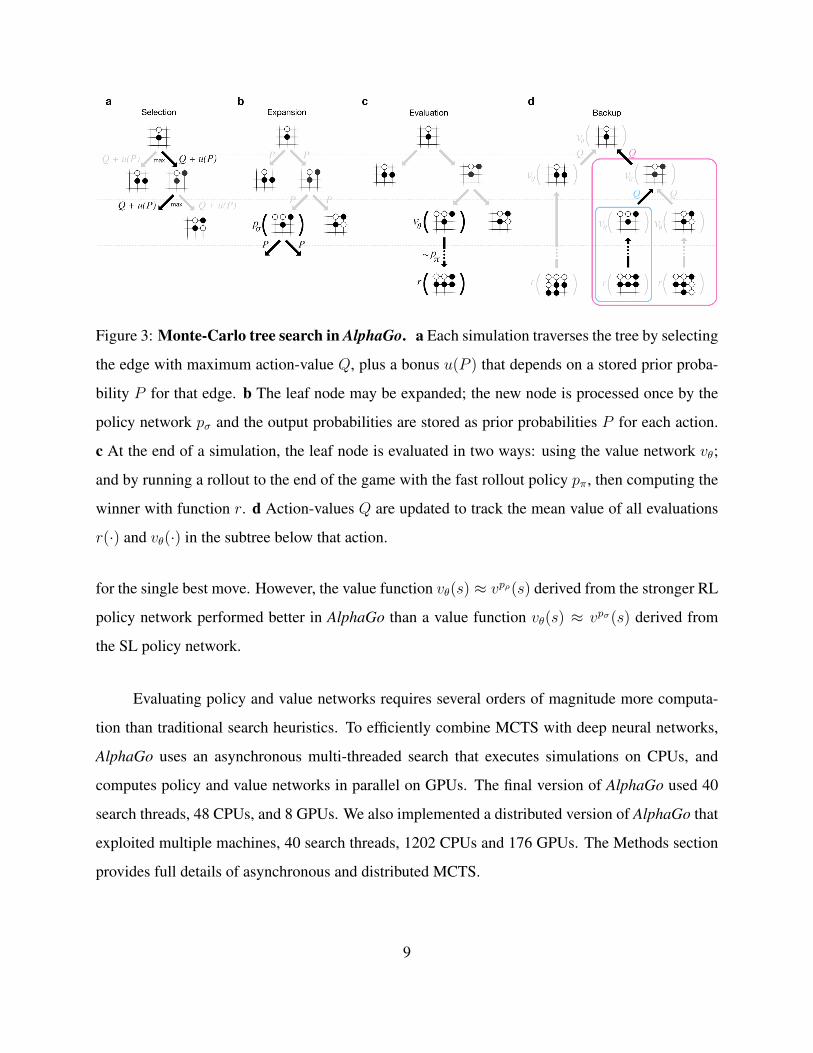
Figure 3: Monte-Carlo tree search in AlphaGo. a Each simulation traverses the tree by selecting

the edge with maximum action-value Q, plus a bonus u(P ) that depends on a stored prior proba-

bility P for that edge. b The leaf node may be expanded; the new node is processed once by the

policy network pσ and the output probabilities are stored as prior probabilities P for each action.

c At the end of a simulation, the leaf node is evaluated in two ways: using the value network vθ;

and by running a rollout to the end of the game with the fast rollout policy pπ, then computing the

winner with function r. d Action-values Q are updated to track the mean value of all evaluations

r(·) and vθ(·) in the subtree below that action.

for the single best move. However, the value function vθ(s) ≈ vpρ(s) derived from the stronger RL

policy network performed better in AlphaGo than a value function vθ(s) ≈ vpσ(s) derived from

the SL policy network.

Evaluating policy and value networks requires several orders of magnitude more computa-

tion than traditional search heuristics. To efficiently combine MCTS with deep neural networks,

AlphaGo uses an asynchronous multi-threaded search that executes simulations on CPUs, and

computes policy and value networks in parallel on GPUs. The final version of AlphaGo used 40

search threads, 48 CPUs, and 8 GPUs. We also implemented a distributed version of AlphaGo that

exploited multiple machines, 40 search threads, 1202 CPUs and 176 GPUs. The Methods section

provides full details of asynchronous and distributed MCTS.

9

5 Evaluating the Playing Strength of AlphaGo

To evaluate AlphaGo, we ran an internal tournament among variants of AlphaGo and several

other Go programs, including the strongest commercial programs Crazy Stone 13 and Zen, and

the strongest open source programs Pachi 14 and Fuego 15. All of these programs are based on

high-performance MCTS algorithms. In addition, we included the open source program GnuGo,

a Go program using state-of-the-art search methods that preceded MCTS. All programs were al-

lowed 5 seconds of computation time per move.

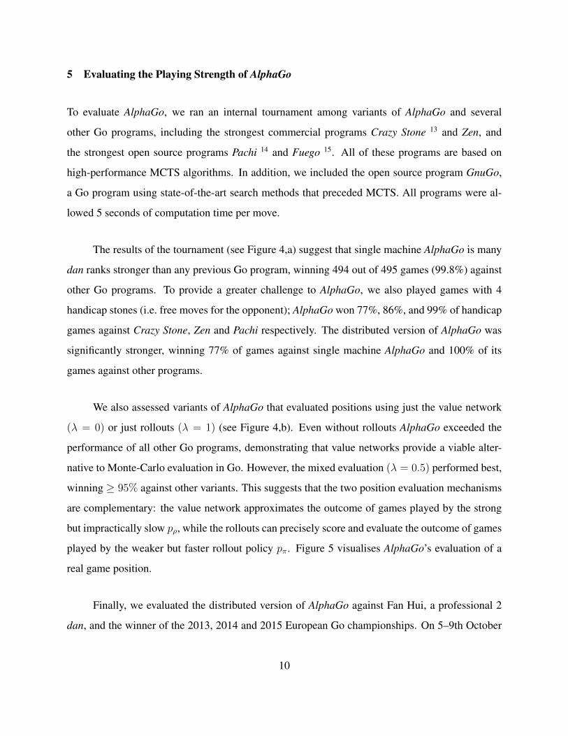
The results of the tournament (see Figure 4,a) suggest that single machine AlphaGo is many

dan ranks stronger than any previous Go program, winning 494 out of 495 games (99.8%) against

other Go programs. To provide a greater challenge to AlphaGo, we also played games with 4

handicap stones (i.e. free moves for the opponent); AlphaGo won 77%, 86%, and 99% of handicap

games against Crazy Stone, Zen and Pachi respectively. The distributed version of AlphaGo was

significantly stronger, winning 77% of games against single machine AlphaGo and 100% of its

games against other programs.

We also assessed variants of AlphaGo that evaluated positions using just the value network

(λ = 0) or just rollouts (λ = 1) (see Figure 4,b). Even without rollouts AlphaGo exceeded the

performance of all other Go programs, demonstrating that value networks provide a viable alter-

native to Monte-Carlo evaluation in Go. However, the mixed evaluation (λ = 0.5) performed best,

winning ≥ 95% against other variants. This suggests that the two position evaluation mechanisms

are complementary: the value network approximates the outcome of games played by the strong

but impractically slow pρ, while the rollouts can precisely score and evaluate the outcome of games

played by the weaker but faster rollout policy pπ. Figure 5 visualises AlphaGo’s evaluation of a

real game position.

Finally, we evaluated the distributed version of AlphaGo against Fan Hui, a professional 2

dan, and the winner of the 2013, 2014 and 2015 European Go championships. On 5–9th October

10

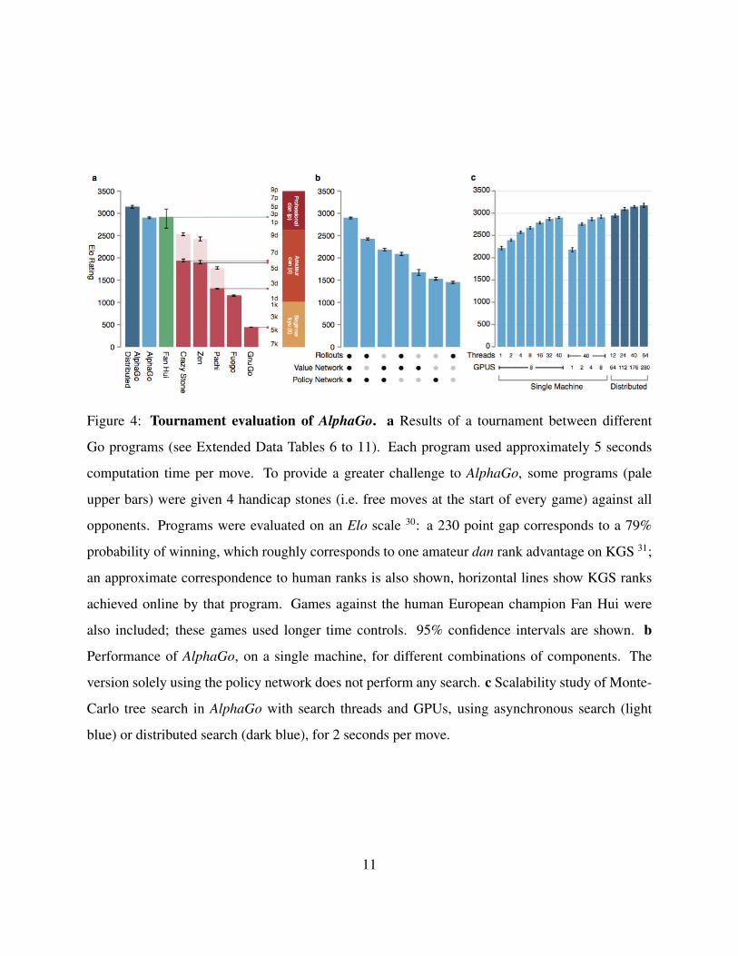
Figure 4: Tournament evaluation of AlphaGo. a Results of a tournament between different

Go programs (see Extended Data Tables 6 to 11). Each program used approximately 5 seconds

computation time per move. To provide a greater challenge to AlphaGo, some programs (pale

upper bars) were given 4 handicap stones (i.e. free moves at the start of every game) against all

opponents. Programs were evaluated on an Elo scale 30: a 230 point gap corresponds to a 79%

probability of winning, which roughly corresponds to one amateur dan rank advantage on KGS 31;

an approximate correspondence to human ranks is also shown, horizontal lines show KGS ranks

achieved online by that program. Games against the human European champion Fan Hui were

also included; these games used longer time controls. 95% confidence intervals are shown. b

Performance of AlphaGo, on a single machine, for different combinations of components. The

version solely using the policy network does not perform any search. c Scalability study of Monte-

Carlo tree search in AlphaGo with search threads and GPUs, using asynchronous search (light

blue) or distributed search (dark blue), for 2 seconds per move.

11

Figure 5: How AlphaGo (black, to play) selected its move in an informal game against Fan

Hui. For each of the following statistics, the location of the maximum value is indicated by an

orange circle. a Evaluation of all successors s′ of the root position s, using the value network

vθ(s′); estimated winning percentages are shown for the top evaluations. b Action-values Q(s, a)

for each edge (s, a) in the tree from root position s; averaged over value network evaluations

only (λ = 0). c Action-values Q(s, a), averaged over rollout evaluations only (λ = 1). d Move

probabilities directly from the SL policy network, pσ(a|s); reported as a percentage (if above

0.1%). e Percentage frequency with which actions were selected from the root during simulations.

f The principal variation (path with maximum visit count) from AlphaGo’s search tree. The moves

are presented in a numbered sequence. AlphaGo selected the move indicated by the red circle;

Fan Hui responded with the move indicated by the white square; in his post-game commentary he

preferred the move (1) predicted by AlphaGo.

12

2015 AlphaGo and Fan Hui competed in a formal five game match. AlphaGo won the match 5

games to 0 (see Figure 6 and Extended Data Table 1). This is the first time that a computer Go

program has defeated a human professional player, without handicap, in the full game of Go; a feat

that was previously believed to be at least a decade away 3, 7, 32.

6 Discussion

In this work we have developed a Go program, based on a combination of deep neural networks and

tree search, that plays at the level of the strongest human players, thereby achieving one of artificial

intelligence’s “grand challenges” 32–34. We have developed, for the first time, effective move se-

lection and position evaluation functions for Go, based on deep neural networks that are trained by

a novel combination of supervised and reinforcement learning. We have introduced a new search

algorithm that successfully combines neural network evaluations with Monte-Carlo rollouts. Our

program AlphaGo integrates these components together, at scale, in a high-performance tree search

engine.

During the match against Fan Hui, AlphaGo evaluated thousands of times fewer positions

than Deep Blue did in its chess match against Kasparov 4; compensating by selecting those posi-

tions more intelligently, using the policy network, and evaluating them more precisely, using the

value network – an approach that is perhaps closer to how humans play. Furthermore, while Deep

Blue relied on a handcrafted evaluation function, AlphaGo’s neural networks are trained directly

from game-play purely through general-purpose supervised and reinforcement learning methods.

Go is exemplary in many ways of the difficulties faced by artificial intelligence 34, 35: a chal-

lenging decision-making task; an intractable search space; and an optimal solution so complex it

appears infeasible to directly approximate using a policy or value function. The previous major

breakthrough in computer Go, the introduction of Monte-Carlo tree search, led to corresponding

advances in many other domains: for example general game-playing, classical planning, partially

observed planning, scheduling, and constraint satisfaction 36, 37. By combining tree search with

13

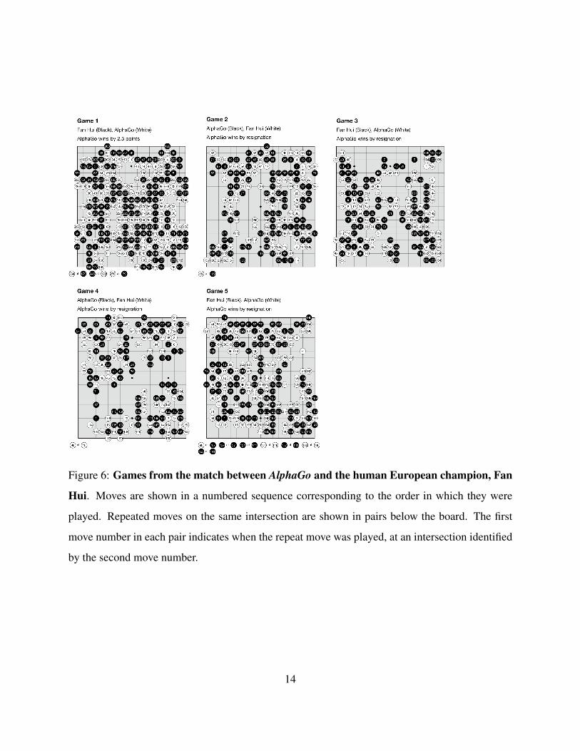
Figure 6: Games from the match between AlphaGo and the human European champion, Fan

Hui. Moves are shown in a numbered sequence corresponding to the order in which they were

played. Repeated moves on the same intersection are shown in pairs below the board. The first

move number in each pair indicates when the repeat move was played, at an intersection identified

by the second move number.

14

policy and value networks, AlphaGo has finally reached a professional level in Go, providing hope

that human-level performance can now be achieved in other seemingly intractable artificial intelli-

gence domains.

References

1. Allis, L. V. Searching for Solutions in Games and Artificial Intelligence. Ph.D. thesis, Univer-

sity of Limburg, Maastricht, The Netherlands (1994).

2. van den Herik, H., Uiterwijk, J. W. & van Rijswijck, J. Games solved: Now and in the future.

Artificial Intelligence 134, 277–311 (2002).

3. Schaeffer, J. The games computers (and people) play. Advances in Computers 50, 189–266

(2000).

4. Campbell, M., Hoane, A. & Hsu, F. Deep Blue. Artificial Intelligence 134, 57–83 (2002).

5. Schaeffer, J. et al. A world championship caliber checkers program. Artificial Intelligence 53,

273–289 (1992).

6. Buro, M. From simple features to sophisticated evaluation functions. In 1st International

Conference on Computers and Games, 126–145 (1999).

7. Muller, M. Computer Go. Artificial Intelligence 134, 145–179 (2002).

8. Tesauro, G. & Galperin, G. On-line policy improvement using Monte-Carlo search. In Ad-

vances in Neural Information Processing, 1068–1074 (1996).

9. Sheppard, B. World-championship-caliber Scrabble. Artificial Intelligence 134, 241–275

(2002).

10. Bouzy, B. & Helmstetter, B. Monte-Carlo Go developments. In 10th International Conference

on Advances in Computer Games, 159–174 (2003).

15

11. Coulom, R. Efficient selectivity and backup operators in Monte-Carlo tree search. In 5th

International Conference on Computer and Games, 72–83 (2006).

12. Kocsis, L. & Szepesvari, C. Bandit based Monte-Carlo planning. In 15th European Conference

on Machine Learning, 282–293 (2006).

13. Coulom, R. Computing Elo ratings of move patterns in the game of Go. International Com-

puter Games Association Journal 30, 198–208 (2007).

14. Baudis, P. & Gailly, J.-L. Pachi: State of the art open source Go program. In Advances in

Computer Games, 24–38 (Springer, 2012).

15. Muller, M., Enzenberger, M., Arneson, B. & Segal, R. Fuego — an open-source framework

for board games and Go engine based on Monte-Carlo tree search. IEEE Transactions on

Computational Intelligence and AI in Games 2, 259–270 (2010).

16. Gelly, S. & Silver, D. Combining online and offline learning in UCT. In 17th International

Conference on Machine Learning, 273–280 (2007).

17. Krizhevsky, A., Sutskever, I. & Hinton, G. ImageNet classification with deep convolutional

neural networks. In Advances in Neural Information Processing Systems, 1097–1105 (2012).

18. Lawrence, S., Giles, C. L., Tsoi, A. C. & Back, A. D. Face recognition: a convolutional

neural-network approach. IEEE Transactions on Neural Networks 8, 98–113 (1997).

19. Mnih, V. et al. Human-level control through deep reinforcement learning. Nature 518, 529–

533 (2015).

20. LeCun, Y., Bengio, Y. & Hinton, G. Deep learning. Nature 521, 436–444 (2015).

21. Stern, D., Herbrich, R. & Graepel, T. Bayesian pattern ranking for move prediction in the

game of Go. In International Conference of Machine Learning, 873–880 (2006).

22. Sutskever, I. & Nair, V. Mimicking Go experts with convolutional neural networks. In Inter-

national Conference on Artificial Neural Networks, 101–110 (2008).

16

23. Maddison, C. J., Huang, A., Sutskever, I. & Silver, D. Move evaluation in Go using deep

convolutional neural networks. 3rd International Conference on Learning Representations

(2015).

24. Clark, C. & Storkey, A. J. Training deep convolutional neural networks to play go. In 32nd

International Conference on Machine Learning, 1766–1774 (2015).

25. Williams, R. J. Simple statistical gradient-following algorithms for connectionist reinforce-

ment learning. Machine Learning 8, 229–256 (1992).

26. Sutton, R., McAllester, D., Singh, S. & Mansour, Y. Policy gradient methods for reinforcement

learning with function approximation. In Advances in Neural Information Processing Systems,

1057–1063 (2000).

27. Schraudolph, N. N., Dayan, P. & Sejnowski, T. J. Temporal difference learning of position

evaluation in the game of Go. Advances in Neural Information Processing Systems 817–817

(1994).

28. Enzenberger, M. Evaluation in Go by a neural network using soft segmentation. In 10th

Advances in Computer Games Conference, 97–108 (2003).

29. Silver, D., Sutton, R. & Muller, M. Temporal-difference search in computer Go. Machine

learning 87, 183–219 (2012).

30. Coulom, R. Whole-history rating: A Bayesian rating system for players of time-varying

strength. In International Conference on Computers and Games, 113–124 (2008).

31. KGS: Rating system math. URL http://www.gokgs.com/help/rmath.html.

32. Levinovitz, A. The mystery of Go, the ancient game that computers still can’t win. Wired

Magazine (2014).

33. Mechner, D. All Systems Go. The Sciences 38 (1998).

17

34. Mandziuk, J. Computational intelligence in mind games. In Challenges for Computational

Intelligence, 407–442 (2007).

35. Berliner, H. A chronology of computer chess and its literature. Artificial Intelligence 10,

201–214 (1978).

36. Browne, C. et al. A survey of Monte-Carlo tree search methods. IEEE Transactions of Com-

putational Intelligence and AI in Games 4, 1–43 (2012).

37. Gelly, S. et al. The grand challenge of computer Go: Monte Carlo tree search and extensions.

Communications of the ACM 55, 106–113 (2012).

Author Contributions

A.H., G.v.d.D., J.S., I.A., M.La., A.G., T.G., D.S. designed and implemented the search in Al-

phaGo. C.M., A.G., L.S., A.H., I.A., V.P., S.D., D.G., N.K., I.S., K.K., D.S. designed and trained

the neural networks in AlphaGo. J.S., J.N., A.H., D.S. designed and implemented the evaluation

framework for AlphaGo. D.S., M.Le., T.L., T.G., K.K., D.H. managed and advised on the project.

D.S., T.G., A.G., D.H. wrote the paper.

Acknowledgements

We thank Fan Hui for agreeing to play against AlphaGo; Toby Manning for refereeing the match;

R. Munos and T. Schaul for helpful discussions and advice; A. Cain and M. Cant for work on

the visuals; P. Dayan, G. Wayne, D. Kumaran, D. Purves, H. van Hasselt, A. Barreto and G.

Ostrovski for reviewing the paper; and the rest of the DeepMind team for their support, ideas and

encouragement.

18

Methods

Problem setting Many games of perfect information, such as chess, checkers, othello, backgam-

mon and Go, may be defined as alternating Markov games 38. In these games, there is a state

space S (where state includes an indication of the current player to play); an action space A(s)

defining the legal actions in any given state s ∈ S; a state transition function f(s, a, ξ) defining

the successor state after selecting action a in state s and random input ξ (e.g. dice); and finally a

reward function ri(s) describing the reward received by player i in state s. We restrict our atten-

tion to two-player zero sum games, r1(s) = −r2(s) = r(s), with deterministic state transitions,

f(s, a, ξ) = f(s, a), and zero rewards except at a terminal time-step T . The outcome of the game

zt = ±r(sT ) is the terminal reward at the end of the game from the perspective of the current

player at time-step t. A policy p(a|s) is a probability distribution over legal actions a ∈ A(s).

A value function is the expected outcome if all actions for both players are selected according to

policy p, that is, vp(s) = E [zt | st = s, at...T ∼ p]. Zero sum games have a unique optimal value

function v∗(s) that determines the outcome from state s following perfect play by both players,

v∗(s) =

zT if s = sT ,

maxa− v∗(f(s, a)) otherwise.

Prior work The optimal value function can be computed recursively by minimax (or equivalently

negamax) search 39. Most games are too large for exhaustive minimax tree search; instead, the

game is truncated by using an approximate value function v(s) ≈ v∗(s) in place of terminal re-

wards. Depth-first minimax search with α − β pruning 39 has achieved super-human performance

in chess 4, checkers 5 and othello 6, but it has not been effective in Go 7.

Reinforcement learning can learn to approximate the optimal value function directly from

games of self-play 38. The majority of prior work has focused on a linear combination vθ(s) =

φ(s) ·θ of features φ(s) with weights θ. Weights were trained using temporal-difference learning 40

in chess 41, 42, checkers 43, 44 and Go 29; or using linear regression in othello 6 and Scrabble 9.

Temporal-difference learning has also been used to train a neural network to approximate the

optimal value function, achieving super-human performance in backgammon 45; and achieving

19

weak kyu level performance in small-board Go 27, 28, 46 using convolutional networks.

An alternative approach to minimax search is Monte-Carlo tree search (MCTS) 11, 12, which

estimates the optimal value of interior nodes by a double approximation, V n(s) ≈ vPn(s) ≈

v∗(s). The first approximation, V n(s) ≈ vPn(s), uses n Monte-Carlo simulations to estimate the

value function of a simulation policy P n. The second approximation, vPn(s) ≈ v∗(s), uses a

simulation policy P n in place of minimax optimal actions. The simulation policy selects actions

according to a search control function argmaxa

(Qn(s, a) + u(s, a)), such as UCT 12, that selects

children with higher action-values,Qn(s, a) = −V n(f(s, a)), plus a bonus u(s, a) that encourages

exploration; or in the absence of a search tree at state s, it samples actions from a fast rollout policy

pπ(a|s). As more simulations are executed and the search tree grows deeper, the simulation policy

becomes informed by increasingly accurate statistics. In the limit, both approximations become

exact and MCTS (e.g., with UCT) converges 12 to the optimal value function limn→∞ Vn(s) =

limn→∞ vPn(s) = v∗(s). The strongest current Go programs are based on MCTS 13–15, 37.

MCTS has previously been combined with a policy that is used to narrow the beam of

the search tree to high probability moves 13; or to bias the bonus term towards high probability

moves 47. MCTS has also been combined with a value function that is used to initialise action-

values in newly expanded nodes 16, or to mix Monte-Carlo evaluation with minimax evaluation 48.

In contrast, AlphaGo’s use of value functions is based on truncated Monte-Carlo search algo-

rithms 8, 9, which terminate rollouts before the end of the game and use a value function in place

of the terminal reward. AlphaGo’s position evaluation mixes full rollouts with truncated rollouts,

resembling in some respects the well-known temporal-difference learning algorithm TD(λ). Al-

phaGo also differs from prior work by using slower but more powerful representations of the

policy and value function; evaluating deep neural networks is several orders of magnitudes slower

than linear representations and must therefore occur asynchronously.

The performance of MCTS is to a large degree determined by the quality of the rollout pol-

icy. Prior work has focused on handcrafted patterns 49 or learning rollout policies by supervised

learning 13, reinforcement learning 16, simulation balancing 50, 51 or online adaptation 29, 52; how-

20

ever, it is known that rollout-based position evaluation is frequently inaccurate 53. AlphaGo uses

relatively simple rollouts, and instead addresses the challenging problem of position evaluation

more directly using value networks.

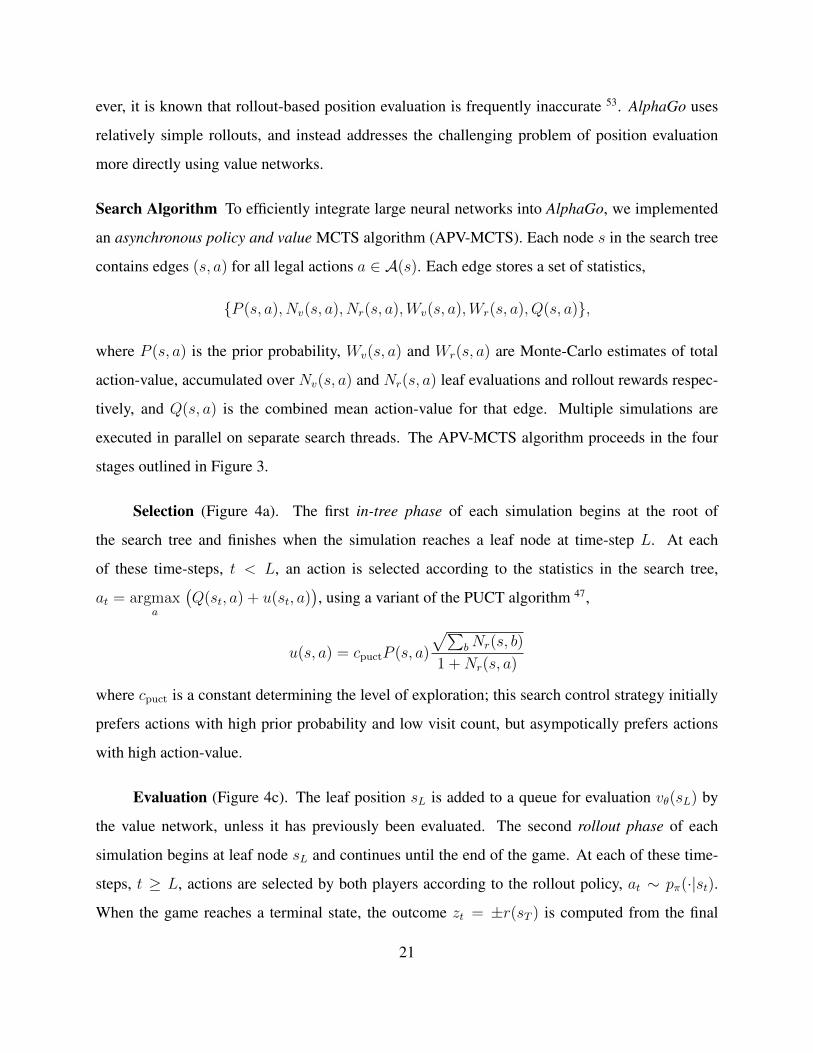
Search Algorithm To efficiently integrate large neural networks into AlphaGo, we implemented

an asynchronous policy and value MCTS algorithm (APV-MCTS). Each node s in the search tree

contains edges (s, a) for all legal actions a ∈ A(s). Each edge stores a set of statistics,

{P (s, a), Nv(s, a), Nr(s, a),Wv(s, a),Wr(s, a), Q(s, a)},

where P (s, a) is the prior probability, Wv(s, a) and Wr(s, a) are Monte-Carlo estimates of total

action-value, accumulated over Nv(s, a) and Nr(s, a) leaf evaluations and rollout rewards respec-

tively, and Q(s, a) is the combined mean action-value for that edge. Multiple simulations are

executed in parallel on separate search threads. The APV-MCTS algorithm proceeds in the four

stages outlined in Figure 3.

Selection (Figure 4a). The first in-tree phase of each simulation begins at the root of

the search tree and finishes when the simulation reaches a leaf node at time-step L. At each

of these time-steps, t < L, an action is selected according to the statistics in the search tree,

at = argmaxa

(Q(st, a) + u(st, a)

), using a variant of the PUCT algorithm 47,

u(s, a) = cpuctP (s, a)

√∑bNr(s, b)

1 +Nr(s, a)

where cpuct is a constant determining the level of exploration; this search control strategy initially

prefers actions with high prior probability and low visit count, but asympotically prefers actions

with high action-value.

Evaluation (Figure 4c). The leaf position sL is added to a queue for evaluation vθ(sL) by

the value network, unless it has previously been evaluated. The second rollout phase of each

simulation begins at leaf node sL and continues until the end of the game. At each of these time-

steps, t ≥ L, actions are selected by both players according to the rollout policy, at ∼ pπ(·|st).

When the game reaches a terminal state, the outcome zt = ±r(sT ) is computed from the final

21

score.

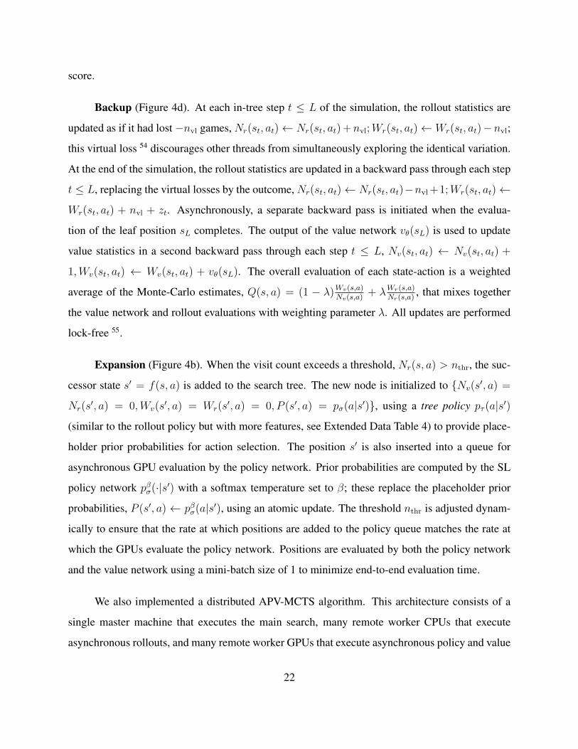
Backup (Figure 4d). At each in-tree step t ≤ L of the simulation, the rollout statistics are

updated as if it had lost −nvl games, Nr(st, at)← Nr(st, at) +nvl;Wr(st, at)← Wr(st, at)−nvl;

this virtual loss 54 discourages other threads from simultaneously exploring the identical variation.

At the end of the simulation, the rollout statistics are updated in a backward pass through each step

t ≤ L, replacing the virtual losses by the outcome, Nr(st, at)← Nr(st, at)−nvl +1;Wr(st, at)←

Wr(st, at) + nvl + zt. Asynchronously, a separate backward pass is initiated when the evalua-

tion of the leaf position sL completes. The output of the value network vθ(sL) is used to update

value statistics in a second backward pass through each step t ≤ L, Nv(st, at) ← Nv(st, at) +

1,Wv(st, at) ← Wv(st, at) + vθ(sL). The overall evaluation of each state-action is a weighted

average of the Monte-Carlo estimates, Q(s, a) = (1 − λ)Wv(s,a)Nv(s,a)

+ λWr(s,a)Nr(s,a)

, that mixes together

the value network and rollout evaluations with weighting parameter λ. All updates are performed

lock-free 55.

Expansion (Figure 4b). When the visit count exceeds a threshold, Nr(s, a) > nthr, the suc-

cessor state s′ = f(s, a) is added to the search tree. The new node is initialized to {Nv(s′, a) =

Nr(s′, a) = 0,Wv(s

′, a) = Wr(s′, a) = 0, P (s′, a) = pσ(a|s′)}, using a tree policy pτ (a|s′)

(similar to the rollout policy but with more features, see Extended Data Table 4) to provide place-

holder prior probabilities for action selection. The position s′ is also inserted into a queue for

asynchronous GPU evaluation by the policy network. Prior probabilities are computed by the SL

policy network pβσ(·|s′) with a softmax temperature set to β; these replace the placeholder prior

probabilities, P (s′, a) ← pβσ(a|s′), using an atomic update. The threshold nthr is adjusted dynam-

ically to ensure that the rate at which positions are added to the policy queue matches the rate at

which the GPUs evaluate the policy network. Positions are evaluated by both the policy network

and the value network using a mini-batch size of 1 to minimize end-to-end evaluation time.

We also implemented a distributed APV-MCTS algorithm. This architecture consists of a

single master machine that executes the main search, many remote worker CPUs that execute

asynchronous rollouts, and many remote worker GPUs that execute asynchronous policy and value

22

network evaluations. The entire search tree is stored on the master, which only executes the in-

tree phase of each simulation. The leaf positions are communicated to the worker CPUs, which

execute the rollout phase of simulation, and to the worker GPUs, which compute network features

and evaluate the policy and value networks. The prior probabilities of the policy network are

returned to the master, where they replace placeholder prior probabilities at the newly expanded

node. The rewards from rollouts and the value network outputs are each returned to the master,

and backed up the originating search path.

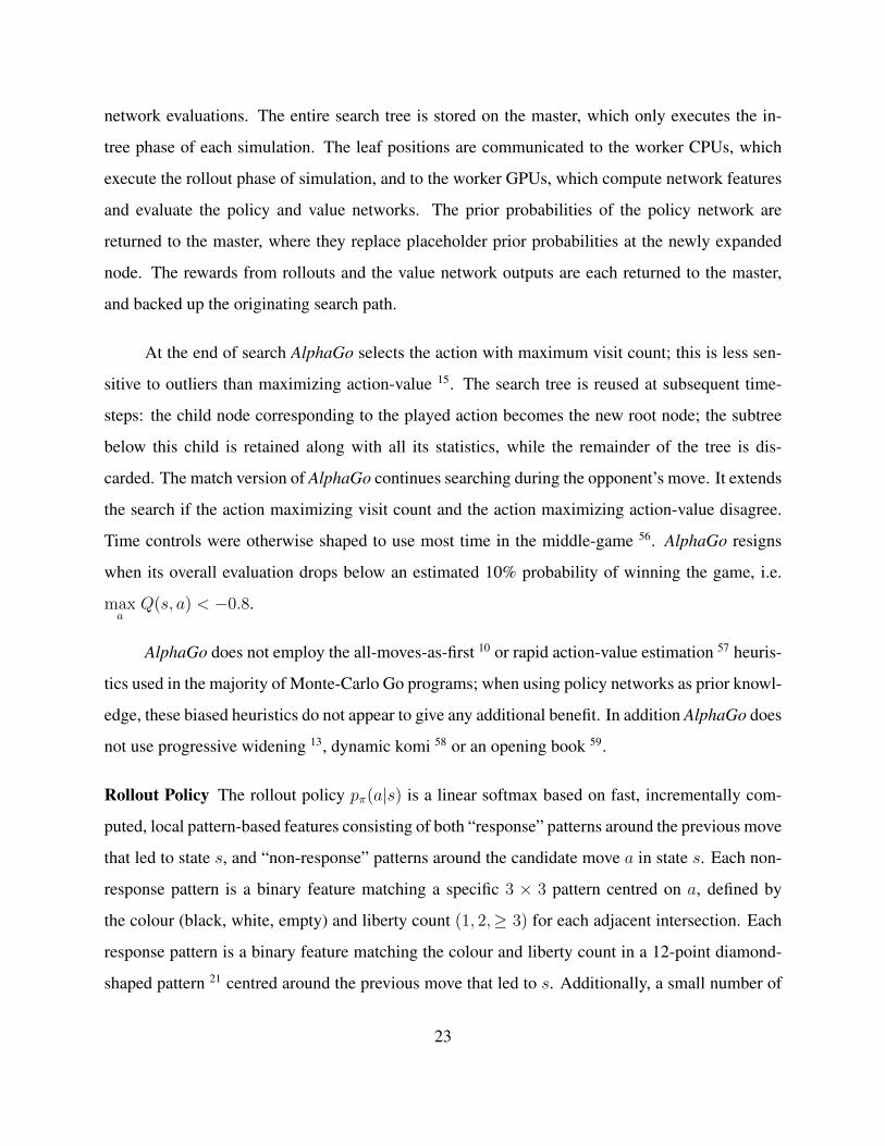
At the end of search AlphaGo selects the action with maximum visit count; this is less sen-

sitive to outliers than maximizing action-value 15. The search tree is reused at subsequent time-

steps: the child node corresponding to the played action becomes the new root node; the subtree

below this child is retained along with all its statistics, while the remainder of the tree is dis-

carded. The match version of AlphaGo continues searching during the opponent’s move. It extends

the search if the action maximizing visit count and the action maximizing action-value disagree.

Time controls were otherwise shaped to use most time in the middle-game 56. AlphaGo resigns

when its overall evaluation drops below an estimated 10% probability of winning the game, i.e.

maxa

Q(s, a) < −0.8.

AlphaGo does not employ the all-moves-as-first 10 or rapid action-value estimation 57 heuris-

tics used in the majority of Monte-Carlo Go programs; when using policy networks as prior knowl-

edge, these biased heuristics do not appear to give any additional benefit. In addition AlphaGo does

not use progressive widening 13, dynamic komi 58 or an opening book 59.

Rollout Policy The rollout policy pπ(a|s) is a linear softmax based on fast, incrementally com-

puted, local pattern-based features consisting of both “response” patterns around the previous move

that led to state s, and “non-response” patterns around the candidate move a in state s. Each non-

response pattern is a binary feature matching a specific 3 × 3 pattern centred on a, defined by

the colour (black, white, empty) and liberty count (1, 2,≥ 3) for each adjacent intersection. Each

response pattern is a binary feature matching the colour and liberty count in a 12-point diamond-

shaped pattern 21 centred around the previous move that led to s. Additionally, a small number of

23

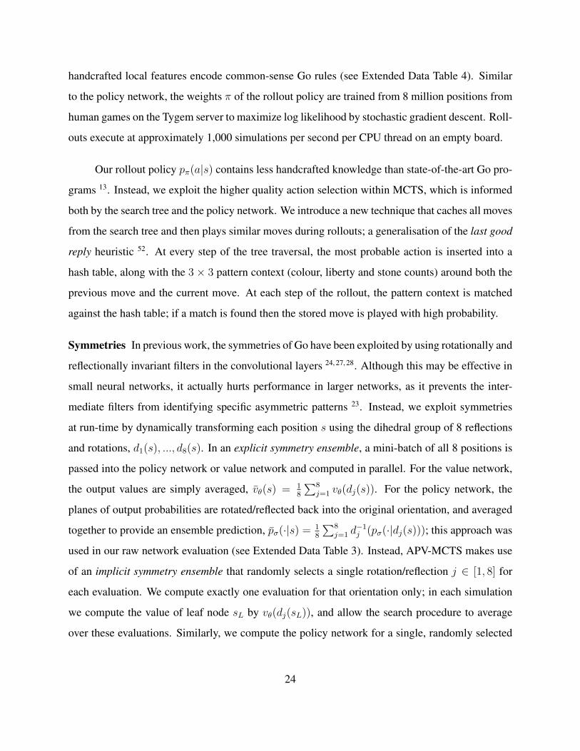
handcrafted local features encode common-sense Go rules (see Extended Data Table 4). Similar

to the policy network, the weights π of the rollout policy are trained from 8 million positions from

human games on the Tygem server to maximize log likelihood by stochastic gradient descent. Roll-

outs execute at approximately 1,000 simulations per second per CPU thread on an empty board.

Our rollout policy pπ(a|s) contains less handcrafted knowledge than state-of-the-art Go pro-

grams 13. Instead, we exploit the higher quality action selection within MCTS, which is informed

both by the search tree and the policy network. We introduce a new technique that caches all moves

from the search tree and then plays similar moves during rollouts; a generalisation of the last good

reply heuristic 52. At every step of the tree traversal, the most probable action is inserted into a

hash table, along with the 3 × 3 pattern context (colour, liberty and stone counts) around both the

previous move and the current move. At each step of the rollout, the pattern context is matched

against the hash table; if a match is found then the stored move is played with high probability.

Symmetries In previous work, the symmetries of Go have been exploited by using rotationally and

reflectionally invariant filters in the convolutional layers 24, 27, 28. Although this may be effective in

small neural networks, it actually hurts performance in larger networks, as it prevents the inter-

mediate filters from identifying specific asymmetric patterns 23. Instead, we exploit symmetries

at run-time by dynamically transforming each position s using the dihedral group of 8 reflections

and rotations, d1(s), ..., d8(s). In an explicit symmetry ensemble, a mini-batch of all 8 positions is

passed into the policy network or value network and computed in parallel. For the value network,

the output values are simply averaged, vθ(s) = 18

∑8j=1 vθ(dj(s)). For the policy network, the

planes of output probabilities are rotated/reflected back into the original orientation, and averaged

together to provide an ensemble prediction, pσ(·|s) = 18

∑8j=1 d

−1j (pσ(·|dj(s))); this approach was

used in our raw network evaluation (see Extended Data Table 3). Instead, APV-MCTS makes use

of an implicit symmetry ensemble that randomly selects a single rotation/reflection j ∈ [1, 8] for

each evaluation. We compute exactly one evaluation for that orientation only; in each simulation

we compute the value of leaf node sL by vθ(dj(sL)), and allow the search procedure to average

over these evaluations. Similarly, we compute the policy network for a single, randomly selected

24

rotation/reflection, d−1j (pσ(·|dj(s))).

Policy Network: Classification We trained the policy network pσ to classify positions according

to expert moves played in the KGS data set. This data set contains 29.4 million positions from

160,000 games played by KGS 6 to 9 dan human players; 35.4% of the games are handicap games.

The data set was split into a test set (the first million positions) and a training set (the remaining

28.4 million positions). Pass moves were excluded from the data set. Each position consisted

of a raw board description s and the move a selected by the human. We augmented the data

set to include all 8 reflections and rotations of each position. Symmetry augmentation and input

features were precomputed for each position. For each training step, we sampled a randomly

selected mini-batch of m samples from the augmented KGS data-set, {sk, ak}mk=1 and applied

an asynchronous stochastic gradient descent update to maximize the log likelihood of the action,

∆σ = αm

∑mk=1

∂log pσ(ak|sk)∂σ

. The step-size α was initialized to 0.003 and was halved every 80

million training steps, without momentum terms, and a mini-batch size of m = 16. Updates

were applied asynchronously on 50 GPUs using DistBelief 60; gradients older than 100 steps were

discarded. Training took around 3 weeks for 340 million training steps.

Policy Network: Reinforcement Learning We further trained the policy network by policy gra-

dient reinforcement learning 25, 26. Each iteration consisted of a mini-batch of n games played in

parallel, between the current policy network pρ that is being trained, and an opponent pρ− that uses

parameters ρ− from a previous iteration, randomly sampled from a pool O of opponents, so as to

increase the stability of training. Weights were initialized to ρ = ρ− = σ. Every 500 iterations, we

added the current parameters ρ to the opponent pool. Each game i in the mini-batch was played

out until termination at step T i, and then scored to determine the outcome zit = ±r(sT i) from

each player’s perspective. The games were then replayed to determine the policy gradient update,

∆ρ = αn

∑ni=1

∑T i

t=1∂log pρ(ait|sit)

∂ρ(zit − v(sit)), using the REINFORCE algorithm 25 with baseline

v(sit) for variance reduction. On the first pass through the training pipeline, the baseline was set

to zero; on the second pass we used the value network vθ(s) as a baseline; this provided a small

performance boost. The policy network was trained in this way for 10,000 mini-batches of 128

25

games, using 50 GPUs, for one day.

Value Network: Regression We trained a value network vθ(s) ≈ vpρ(s) to approximate the value

function of the RL policy network pρ. To avoid overfitting to the strongly correlated positions

within games, we constructed a new data-set of uncorrelated self-play positions. This data-set

consisted of over 30 million positions, each drawn from a unique game of self-play. Each game

was generated in three phases by randomly sampling a time-step U ∼ unif{1, 450}, and sampling

the first t = 1, ..., U−1 moves from the SL policy network, at ∼ pσ(·|st); then sampling one move

uniformly at random from available moves, aU ∼ unif{1, 361} (repeatedly until aU is legal); then

sampling the remaining sequence of moves until the game terminates, t = U + 1, ..., T , from

the RL policy network, at ∼ pρ(·|st). Finally, the game is scored to determine the outcome zt =

±r(sT ). Only a single training example (sU+1, zU+1) is added to the data-set from each game. This

data provides unbiased samples of the value function vpρ(sU+1) = E [zU+1 | sU+1, aU+1,...,T ∼ pρ].

During the first two phases of generation we sample from noisier distributions so as to increase the

diversity of the data-set. The training method was identical to SL policy network training, except

that the parameter update was based on mean squared error between the predicted values and the

observed rewards, ∆θ = αm

∑mk=1

(zk − vθ(s

k))∂vθ(sk)

∂θ. The value network was trained for 50

million mini-batches of 32 positions, using 50 GPUs, for one week.

Features for Policy / Value Network Each position s was preprocessed into a set of 19 × 19

feature planes. The features that we use come directly from the raw representation of the game

rules, indicating the status of each intersection of the Go board: stone colour, liberties (adjacent

empty points of stone’s chain), captures, legality, turns since stone was played, and (for the value

network only) the current colour to play. In addition, we use one simple tactical feature that

computes the outcome of a ladder search 7. All features were computed relative to the current

colour to play; for example, the stone colour at each intersection was represented as either player

or opponent rather than black or white. Each integer is split into K different 19 × 19 planes of

binary values (one-hot encoding). For example, separate binary feature planes are used to represent

whether an intersection has 1 liberty, 2 liberties, ..., ≥ 8 liberties. The full set of feature planes are

26

listed in Extended Data Table 2.

Neural Network Architecture The input to the policy network is a 19 × 19 × 48 image stack

consisting of 48 feature planes. The first hidden layer zero pads the input into a 23 × 23 image,

then convolves k filters of kernel size 5×5 with stride 1 with the input image and applies a rectifier

nonlinearity. Each of the subsequent hidden layers 2 to 12 zero pads the respective previous hidden

layer into a 21×21 image, then convolves k filters of kernel size 3×3 with stride 1, again followed

by a rectifier nonlinearity. The final layer convolves 1 filter of kernel size 1× 1 with stride 1, with

a different bias for each position, and applies a softmax function. The match version of AlphaGo

used k = 192 filters; Figure 2,b and Extended Data Table 3 additionally show the results of training

with k = 128, 256, 384 filters.

The input to the value network is also a 19× 19× 48 image stack, with an additional binary

feature plane describing the current colour to play. Hidden layers 2 to 11 are identical to the policy

network, hidden layer 12 is an additional convolution layer, hidden layer 13 convolves 1 filter of

1 × 1 with stride 1, and hidden layer 14 is a fully connected linear layer with 256 rectifier units.

The output layer is a fully connected linear layer with a single tanh unit.

Evaluation We evaluated the relative strength of computer Go programs by running an internal

tournament and measuring the Elo rating of each program. We estimate the probability that pro-

gram a will beat program b by a logistic function p(a beats b) = 11+exp(celo(e(b)−e(a))

, and estimate

the ratings e(·) by Bayesian logistic regression, computed by the BayesElo program 30 using the

standard constant celo = 1/400. The scale was anchored to the BayesElo rating of professional Go

player Fan Hui (2908 at date of submission) 61. All programs received a maximum of 5 seconds

computation time per move; games were scored using Chinese rules with a komi of 7.5 points (extra

points to compensate white for playing second). We also played handicap games where AlphaGo

played white against existing Go programs; for these games we used a non-standard handicap sys-

tem in which komi was retained but black was given additional stones on the usual handicap points.

Using these rules, a handicap of K stones is equivalent to giving K− 1 free moves to black, rather

than K − 1/2 free moves using standard no-komi handicap rules. We used these handicap rules

27

because AlphaGo’s value network was trained specifically to use a komi of 7.5.

With the exception of distributed AlphaGo, each computer Go program was executed on its

own single machine, with identical specs, using the latest available version and the best hardware

configuration supported by that program (see Extended Data Table 6). In Figure 4, approximate

ranks of computer programs are based on the highest KGS rank achieved by that program; however,

the KGS version may differ from the publicly available version.

The match against Fan Hui was arbitrated by an impartial referee. 5 formal games and 5

informal games were played with 7.5 komi, no handicap, and Chinese rules. AlphaGo won these

games 5–0 and 3–2 respectively (Figure 6 and Extended Data Figure 6). Time controls for formal

games were 1 hour main time plus 3 periods of 30 seconds byoyomi. Time controls for informal

games were 3 periods of 30 seconds byoyomi. Time controls and playing conditions were chosen

by Fan Hui in advance of the match; it was also agreed that the overall match outcome would be

determined solely by the formal games. To approximately assess the relative rating of Fan Hui to

computer Go programs, we appended the results of all 10 games to our internal tournament results,

ignoring differences in time controls.

References

38. Littman, M. L. Markov games as a framework for multi-agent reinforcement learning. In 11th

International Conference on Machine Learning, 157–163 (1994).

39. Knuth, D. E. & Moore, R. W. An analysis of alpha-beta pruning. Artificial Intelligence 6,

293–326 (1975).

40. Sutton, R. Learning to predict by the method of temporal differences. Machine Learning 3,

9–44 (1988).

41. Baxter, J., Tridgell, A. & Weaver, L. Learning to play chess using temporal differences.

Machine Learning 40, 243–263 (2000).

28

42. Veness, J., Silver, D., Blair, A. & Uther, W. Bootstrapping from game tree search. In Advances

in Neural Information Processing Systems (2009).

43. Samuel, A. L. Some studies in machine learning using the game of checkers II - recent

progress. IBM Journal of Research and Development 11, 601–617 (1967).

44. Schaeffer, J., Hlynka, M. & Jussila, V. Temporal difference learning applied to a high-

performance game-playing program. In 17th International Joint Conference on Artificial In-

telligence, 529–534 (2001).

45. Tesauro, G. TD-gammon, a self-teaching backgammon program, achieves master-level play.

Neural Computation 6, 215–219 (1994).

46. Dahl, F. Honte, a Go-playing program using neural nets. In Machines that learn to play games,

205–223 (Nova Science, 1999).

47. Rosin, C. D. Multi-armed bandits with episode context. Annals of Mathematics and Artificial

Intelligence 61, 203–230 (2011).

48. Lanctot, M., Winands, M. H. M., Pepels, T. & Sturtevant, N. R. Monte Carlo tree search with

heuristic evaluations using implicit minimax backups. In IEEE Conference on Computational

Intelligence and Games, 1–8 (2014).

49. Gelly, S., Wang, Y., Munos, R. & Teytaud, O. Modification of UCT with patterns in Monte-

Carlo Go. Tech. Rep. 6062, INRIA (2006).

50. Silver, D. & Tesauro, G. Monte-Carlo simulation balancing. In 26th International Conference

on Machine Learning, 119 (2009).

51. Huang, S.-C., Coulom, R. & Lin, S.-S. Monte-Carlo simulation balancing in practice. In 7th

International Conference on Computers and Games, 81–92 (Springer-Verlag, 2011).

52. Baier, H. & Drake, P. D. The power of forgetting: Improving the last-good-reply policy in

Monte Carlo Go. IEEE Transactions on Computational Intelligence and AI in Games 2, 303–

309 (2010).

29

53. Huang, S. & Muller, M. Investigating the limits of Monte-Carlo tree search methods in com-

puter Go. In 8th International Conference on Computers and Games, 39–48 (2013).

54. Segal, R. B. On the scalability of parallel UCT. Computers and Games 6515, 36–47 (2011).

55. Enzenberger, M. & Muller, M. A lock-free multithreaded Monte-Carlo tree search algorithm.

In 12th Advances in Computer Games Conference, 14–20 (2009).

56. Huang, S.-C., Coulom, R. & Lin, S.-S. Time management for Monte-Carlo tree search applied

to the game of Go. In International Conference on Technologies and Applications of Artificial

Intelligence, 462–466 (2010).

57. Gelly, S. & Silver, D. Monte-Carlo tree search and rapid action value estimation in computer

Go. Artificial Intelligence 175, 1856–1875 (2011).

58. Baudis, P. Balancing MCTS by dynamically adjusting the komi value. International Computer

Games Association 34, 131 (2011).

59. Baier, H. & Winands, M. H. Active opening book application for Monte-Carlo tree search in

19× 19 Go. In Benelux Conference on Artificial Intelligence, 3–10 (2011).

60. Dean, J. et al. Large scale distributed deep networks. In Advances in Neural Information

Processing Systems, 1223–1231 (2012).

61. Go ratings. URL http://www.goratings.org.

30

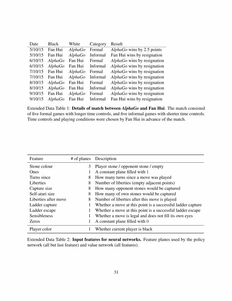
Date Black White Category Result5/10/15 Fan Hui AlphaGo Formal AlphaGo wins by 2.5 points5/10/15 Fan Hui AlphaGo Informal Fan Hui wins by resignation6/10/15 AlphaGo Fan Hui Formal AlphaGo wins by resignation6/10/15 AlphaGo Fan Hui Informal AlphaGo wins by resignation7/10/15 Fan Hui AlphaGo Formal AlphaGo wins by resignation7/10/15 Fan Hui AlphaGo Informal AlphaGo wins by resignation8/10/15 AlphaGo Fan Hui Formal AlphaGo wins by resignation8/10/15 AlphaGo Fan Hui Informal AlphaGo wins by resignation9/10/15 Fan Hui AlphaGo Formal AlphaGo wins by resignation9/10/15 AlphaGo Fan Hui Informal Fan Hui wins by resignation

Extended Data Table 1: Details of match between AlphaGo and Fan Hui. The match consistedof five formal games with longer time controls, and five informal games with shorter time controls.Time controls and playing conditions were chosen by Fan Hui in advance of the match.

Feature # of planes Description

Stone colour 3 Player stone / opponent stone / emptyOnes 1 A constant plane filled with 1Turns since 8 How many turns since a move was playedLiberties 8 Number of liberties (empty adjacent points)Capture size 8 How many opponent stones would be capturedSelf-atari size 8 How many of own stones would be capturedLiberties after move 8 Number of liberties after this move is playedLadder capture 1 Whether a move at this point is a successful ladder captureLadder escape 1 Whether a move at this point is a successful ladder escapeSensibleness 1 Whether a move is legal and does not fill its own eyesZeros 1 A constant plane filled with 0

Player color 1 Whether current player is black

Extended Data Table 2: Input features for neural networks. Feature planes used by the policynetwork (all but last feature) and value network (all features).

31

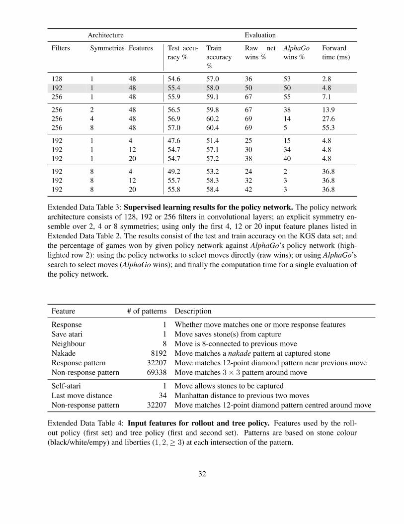
Architecture Evaluation

Filters Symmetries Features Test accu-racy %

Trainaccuracy%

Raw netwins %

AlphaGowins %

Forwardtime (ms)

128 1 48 54.6 57.0 36 53 2.8192 1 48 55.4 58.0 50 50 4.8256 1 48 55.9 59.1 67 55 7.1

256 2 48 56.5 59.8 67 38 13.9256 4 48 56.9 60.2 69 14 27.6256 8 48 57.0 60.4 69 5 55.3

192 1 4 47.6 51.4 25 15 4.8192 1 12 54.7 57.1 30 34 4.8192 1 20 54.7 57.2 38 40 4.8

192 8 4 49.2 53.2 24 2 36.8192 8 12 55.7 58.3 32 3 36.8192 8 20 55.8 58.4 42 3 36.8

Extended Data Table 3: Supervised learning results for the policy network. The policy networkarchitecture consists of 128, 192 or 256 filters in convolutional layers; an explicit symmetry en-semble over 2, 4 or 8 symmetries; using only the first 4, 12 or 20 input feature planes listed inExtended Data Table 2. The results consist of the test and train accuracy on the KGS data set; andthe percentage of games won by given policy network against AlphaGo’s policy network (high-lighted row 2): using the policy networks to select moves directly (raw wins); or using AlphaGo’ssearch to select moves (AlphaGo wins); and finally the computation time for a single evaluation ofthe policy network.

Feature # of patterns Description

Response 1 Whether move matches one or more response featuresSave atari 1 Move saves stone(s) from captureNeighbour 8 Move is 8-connected to previous moveNakade 8192 Move matches a nakade pattern at captured stoneResponse pattern 32207 Move matches 12-point diamond pattern near previous moveNon-response pattern 69338 Move matches 3× 3 pattern around move

Self-atari 1 Move allows stones to be capturedLast move distance 34 Manhattan distance to previous two movesNon-response pattern 32207 Move matches 12-point diamond pattern centred around move

Extended Data Table 4: Input features for rollout and tree policy. Features used by the roll-out policy (first set) and tree policy (first and second set). Patterns are based on stone colour(black/white/empy) and liberties (1, 2,≥ 3) at each intersection of the pattern.

32

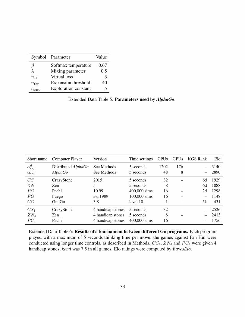
Symbol Parameter Value

β Softmax temperature 0.67λ Mixing parameter 0.5nvl Virtual loss 3nthr Expansion threshold 40cpuct Exploration constant 5

Extended Data Table 5: Parameters used by AlphaGo.

Short name Computer Player Version Time settings CPUs GPUs KGS Rank Elo

αdrvp Distributed AlphaGo See Methods 5 seconds 1202 176 – 3140αrvp AlphaGo See Methods 5 seconds 48 8 – 2890

CS CrazyStone 2015 5 seconds 32 – 6d 1929ZN Zen 5 5 seconds 8 – 6d 1888PC Pachi 10.99 400,000 sims 16 – 2d 1298FG Fuego svn1989 100,000 sims 16 – – 1148GG GnuGo 3.8 level 10 1 – 5k 431

CS4 CrazyStone 4 handicap stones 5 seconds 32 – – 2526ZN4 Zen 4 handicap stones 5 seconds 8 – – 2413PC4 Pachi 4 handicap stones 400,000 sims 16 – – 1756

Extended Data Table 6: Results of a tournament between different Go programs. Each programplayed with a maximum of 5 seconds thinking time per move; the games against Fan Hui wereconducted using longer time controls, as described in Methods. CS4, ZN4 and PC4 were given 4handicap stones; komi was 7.5 in all games. Elo ratings were computed by BayesElo.

33

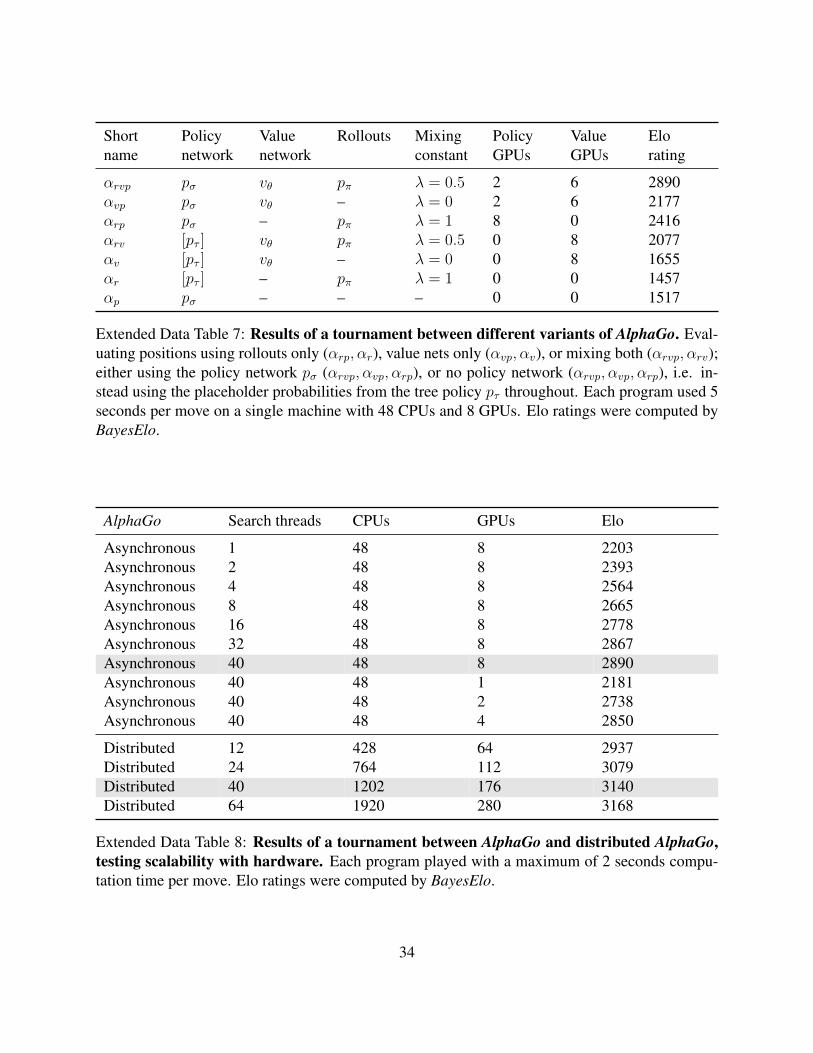
Short Policy Value Rollouts Mixing Policy Value Eloname network network constant GPUs GPUs rating

αrvp pσ vθ pπ λ = 0.5 2 6 2890αvp pσ vθ – λ = 0 2 6 2177αrp pσ – pπ λ = 1 8 0 2416αrv [pτ ] vθ pπ λ = 0.5 0 8 2077αv [pτ ] vθ – λ = 0 0 8 1655αr [pτ ] – pπ λ = 1 0 0 1457αp pσ – – – 0 0 1517

Extended Data Table 7: Results of a tournament between different variants of AlphaGo. Eval-uating positions using rollouts only (αrp, αr), value nets only (αvp, αv), or mixing both (αrvp, αrv);either using the policy network pσ (αrvp, αvp, αrp), or no policy network (αrvp, αvp, αrp), i.e. in-stead using the placeholder probabilities from the tree policy pτ throughout. Each program used 5seconds per move on a single machine with 48 CPUs and 8 GPUs. Elo ratings were computed byBayesElo.

AlphaGo Search threads CPUs GPUs Elo

Asynchronous 1 48 8 2203Asynchronous 2 48 8 2393Asynchronous 4 48 8 2564Asynchronous 8 48 8 2665Asynchronous 16 48 8 2778Asynchronous 32 48 8 2867Asynchronous 40 48 8 2890Asynchronous 40 48 1 2181Asynchronous 40 48 2 2738Asynchronous 40 48 4 2850

Distributed 12 428 64 2937Distributed 24 764 112 3079Distributed 40 1202 176 3140Distributed 64 1920 280 3168

Extended Data Table 8: Results of a tournament between AlphaGo and distributed AlphaGo,testing scalability with hardware. Each program played with a maximum of 2 seconds compu-tation time per move. Elo ratings were computed by BayesElo.

34

αrvp αvp αrp αrv αr αv αp

αrvp - 1 [0; 5] 5 [4; 7] 0 [0; 4] 0 [0; 8] 0 [0; 19] 0 [0; 19]

αvp 99 [95; 100] - 61 [52; 69] 35 [25; 48] 6 [1; 27] 0 [0; 22] 1 [0; 6]

αrp 95 [93; 96] 39 [31; 48] - 13 [7; 23] 0 [0; 9] 0 [0; 22] 4 [1; 21]

αrv 100 [96; 100] 65 [52; 75] 87 [77; 93] - 0 [0; 18] 29 [8; 64] 48 [33; 65]

αr 100 [92; 100] 94 [73; 99] 100 [91; 100] 100 [82; 100] - 78 [45; 94] 78 [71; 84]

αv 100 [81; 100] 100 [78; 100] 100 [78; 100] 71 [36; 92] 22 [6; 55] - 30 [16; 48]

αp 100 [81; 100] 99 [94; 100] 96 [79; 99] 52 [35; 67] 22 [16; 29] 70 [52; 84] -

CS 100 [97; 100] 74 [66; 81] 98 [94; 99] 80 [70; 87] 5 [3; 7] 36 [16; 61] 8 [5; 14]

ZN 99 [93; 100] 84 [67; 93] 98 [93; 99] 92 [67; 99] 6 [2; 19] 40 [12; 77] 100 [65; 100]

PC 100 [98; 100] 99 [95; 100] 100 [98; 100] 98 [89; 100] 78 [73; 81] 87 [68; 95] 55 [47; 62]

FG 100 [97; 100] 99 [93; 100] 100 [96; 100] 100 [91; 100] 78 [73; 83] 100 [65; 100] 65 [55; 73]

GG 100 [44; 100] 100 [34; 100] 100 [68; 100] 100 [57; 100] 99 [97; 100] 67 [21; 94] 99 [95; 100]

CS4 77 [69; 84] 12 [8; 18] 53 [44; 61] 15 [8; 24] 0 [0; 3] 0 [0; 30] 0 [0; 8]

ZN4 86 [77; 92] 25 [16; 38] 67 [56; 76] 14 [7; 27] 0 [0; 12] 0 [0; 43] -

PC4 99 [97; 100] 82 [75; 88] 98 [95; 99] 89 [79; 95] 32 [26; 39] 13 [3; 36] 35 [25; 46]

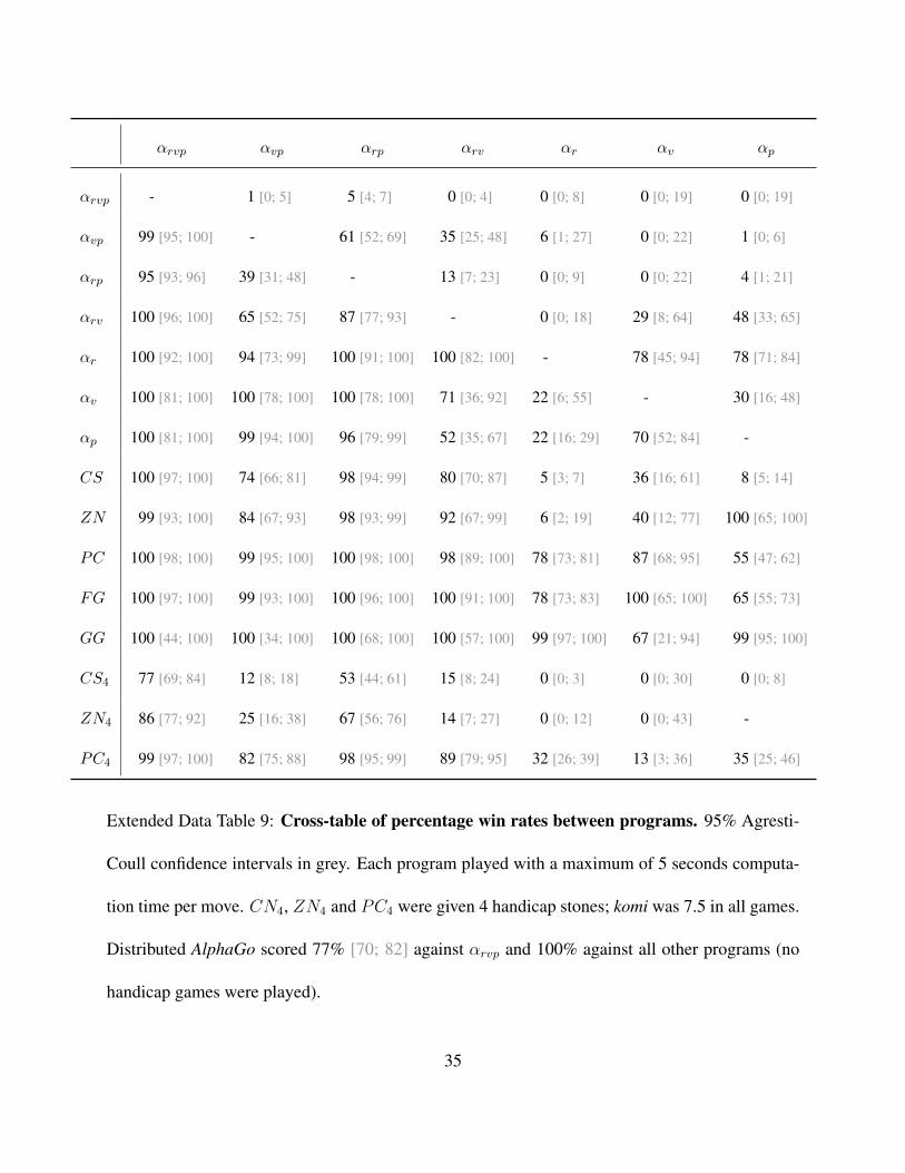
Extended Data Table 9: Cross-table of percentage win rates between programs. 95% Agresti-

Coull confidence intervals in grey. Each program played with a maximum of 5 seconds computa-

tion time per move. CN4, ZN4 and PC4 were given 4 handicap stones; komi was 7.5 in all games.

Distributed AlphaGo scored 77% [70; 82] against αrvp and 100% against all other programs (no

handicap games were played).

35

Threads 1 2 4 8 16 32 40 40 40 40

GPU 8 8 8 8 8 8 8 4 2 1

1 8 - 70 [61;78] 90 [84;94] 94 [83;98] 86 [72;94] 98 [91;100] 98 [92;99] 100 [76;100] 96 [91;98] 38 [25;52]

2 8 30 [22;39] - 72 [61;81] 81 [71;88] 86 [76;93] 92 [83;97] 93 [86;96] 83 [69;91] 84 [75;90] 26 [17;38]

4 8 10 [6;16] 28 [19;39] - 62 [53;70] 71 [61;80] 82 [71;89] 84 [74;90] 81 [69;89] 78 [63;88] 18 [10;28]

8 8 6 [2;17] 19 [12;29] 38 [30;47] - 61 [51;71] 65 [51;76] 73 [62;82] 74 [59;85] 64 [55;73] 12 [3;34]

16 8 14 [6;28] 14 [7;24] 29 [20;39] 39 [29;49] - 52 [41;63] 61 [50;71] 52 [41;64] 41 [32;51] 5 [1;25]

32 8 2 [0;9] 8 [3;17] 18 [11;29] 35 [24;49] 48 [37;59] - 52 [42;63] 44 [32;57] 26 [17;36] 0 [0;30]

40 8 2 [1;8] 7 [4;14] 16 [10;26] 27 [18;38] 39 [29;50] 48 [37;58] - 43 [30;56] 41 [26;58] 4 [1;18]

40 4 0 [0;24] 17 [9;31] 19 [11;31] 26 [15;41] 48 [36;59] 56 [43;68] 57 [44;70] - 29 [18;41] 2 [0;11]

40 2 4 [2;9] 16 [10;25] 22 [12;37] 36 [27;45] 59 [49;68] 74 [64;83] 59 [42;74] 71 [59;82] - 5 [1;17]

40 1 62 [48;75] 74 [62;83] 82 [72;90] 88 [66;97] 95 [75;99] 100 [70;100] 96 [82;99] 98 [89;100] 95 [83;99] -

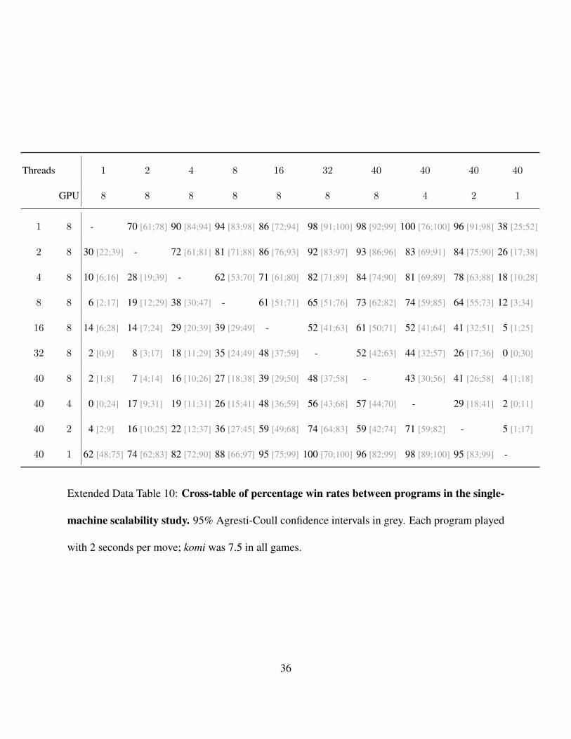
Extended Data Table 10: Cross-table of percentage win rates between programs in the single-

machine scalability study. 95% Agresti-Coull confidence intervals in grey. Each program played

with 2 seconds per move; komi was 7.5 in all games.

36

Threads 40 12 24 40 64

GPU 8 64 112 176 280

CPU 48 428 764 1202 1920

40 8 48 - 52 [43; 61] 68 [59; 76] 77 [70; 82] 81 [65; 91]

12 64 428 48 [39; 57] - 64 [54; 73] 62 [41; 79] 83 [55; 95]

24 112 764 32 [24; 41] 36 [27; 46] - 36 [20; 57] 60 [51; 69]

40 176 1202 23 [18; 30] 38 [21; 59] 64 [43; 80] - 53 [39; 67]

64 280 1920 19 [9; 35] 17 [5; 45] 40 [31; 49] 47 [33; 61] -

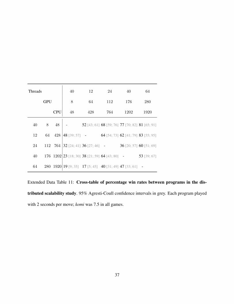
Extended Data Table 11: Cross-table of percentage win rates between programs in the dis-

tributed scalability study. 95% Agresti-Coull confidence intervals in grey. Each program played

with 2 seconds per move; komi was 7.5 in all games.

37