Feedback Vertex Set

Feedback Vertex Set

AAGA ProjectUniversity of Pierre et Marie Curie

NADARAJAH Mag-Stellon

Contents

1 Introduction 1

2 Strategies 22.1 Naive Algorithm . . . . . . . . . . . . . . . . . . . . . . . . . . . . . . . . . 22.2 Fixed Parameter Tractable . . . . . . . . . . . . . . . . . . . . . . . . . . . . 2

2.2.1 Definitions and notations . . . . . . . . . . . . . . . . . . . . . . . . . 22.2.2 Algorithm . . . . . . . . . . . . . . . . . . . . . . . . . . . . . . . . . 32.2.3 Example . . . . . . . . . . . . . . . . . . . . . . . . . . . . . . . . . . 5

2.3 Disjoint-FVS . . . . . . . . . . . . . . . . . . . . . . . . . . . . . . . . . . . 72.3.1 Definitions et notations . . . . . . . . . . . . . . . . . . . . . . . . . . 72.3.2 Algorithm . . . . . . . . . . . . . . . . . . . . . . . . . . . . . . . . . 7

2.4 2-Approximation . . . . . . . . . . . . . . . . . . . . . . . . . . . . . . . . . 92.4.1 Definitions and notations . . . . . . . . . . . . . . . . . . . . . . . . . 92.4.2 Algorithm . . . . . . . . . . . . . . . . . . . . . . . . . . . . . . . . . 92.4.3 Example . . . . . . . . . . . . . . . . . . . . . . . . . . . . . . . . . . 10

2.5 Randomized Algorithm . . . . . . . . . . . . . . . . . . . . . . . . . . . . . . 112.5.1 Definitions et notations . . . . . . . . . . . . . . . . . . . . . . . . . . 112.5.2 Algorithm . . . . . . . . . . . . . . . . . . . . . . . . . . . . . . . . . 11

3 Conclusion 13

4 References 14

1. Introduction

This paper deals with one of the first NP complete problems : FeedBack Vertex Set.

NP complete category problems are hard to solve. In general, algorithms providing a solutionto a problem of these are rather slow. That’s why, these solutions are unusable in practice(although on a reduced instance of a problem).However, it is possible to verify a solution to a NP complete problems in polynomial time.

At present, we know that it is sufficient to find a polynomial solution to a NP-completeproblem in order to solve them all. This is the subject of the biggest computer science prob-lem : P versus NP.

In the rest of this paper, we will analyze different algorithms to solve this problem. FVSis the subject of much research (still ongoing), solutions provide an improvement in timecomplexity (they tend to Θ(polynomial)).

What is FVS ? This is a problem related to cyclic graph. The goal is to find a mini-mum number of nodes "playing a role" in cycles of a graph. By removing these nodes of thegraph is obtained an acyclic graph. More formally, FVS is the set of N nodes of a cyclicgraph G whose deletion makes the graph G acyclic.

This problem is a major problem in combinatorial optimization. It is frequently encoun-tered in operating systems, databases (management of deadlocks), creation of printed circuits(VLSI), compilers optimizing ...

2. Strategies

2.1 Naive Algorithm

A naive algorithm is often an intuitive solution. Here, it would be to test all combinationsC of vertices of graph G. If G− C makes G acyclic then C is a FV S of G.

This approach is set aside in view of its time complexity elevated.

2.2 Fixed Parameter Tractable

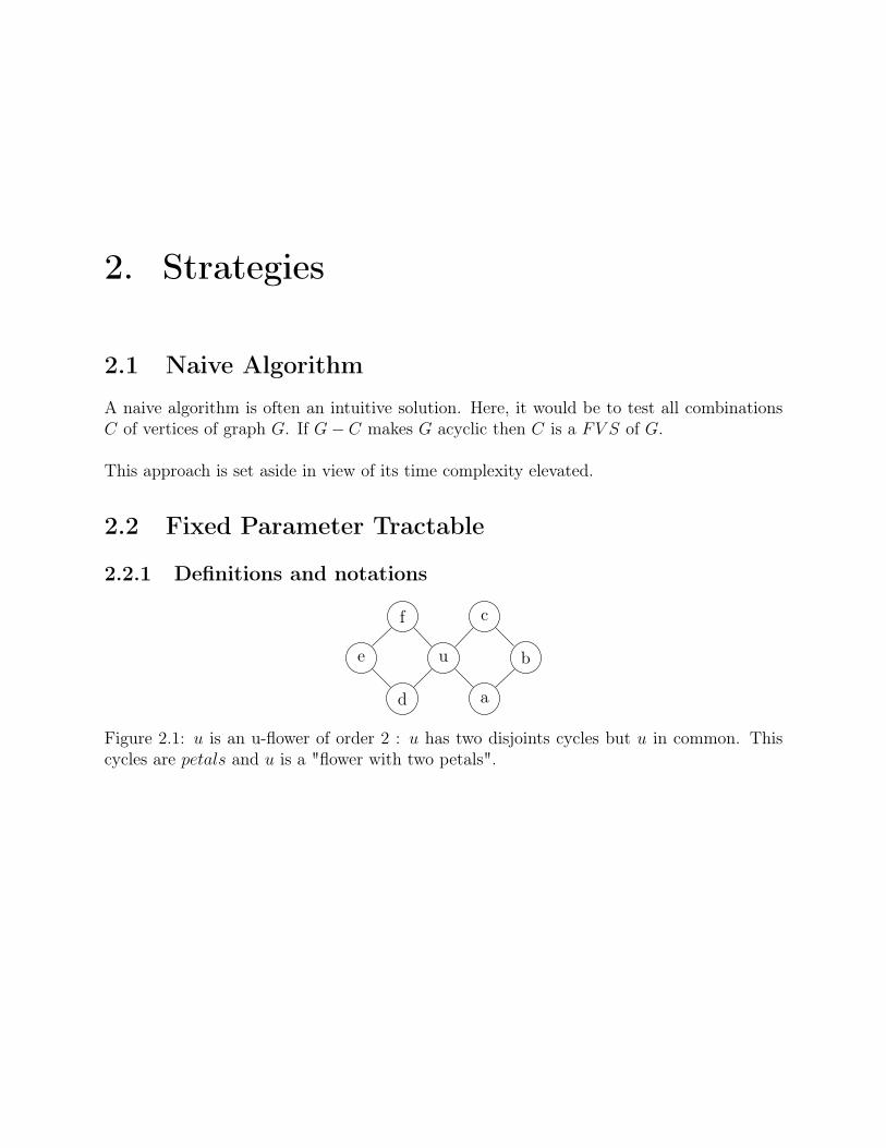
2.2.1 Definitions and notations

u

a

b

c

d

e

f

Figure 2.1: u is an u-flower of order 2 : u has two disjoints cycles but u in common. Thiscycles are petals and u is a "flower with two petals".

2.2 Fixed Parameter Tractable 3

ts

a

b

c

d

e

f

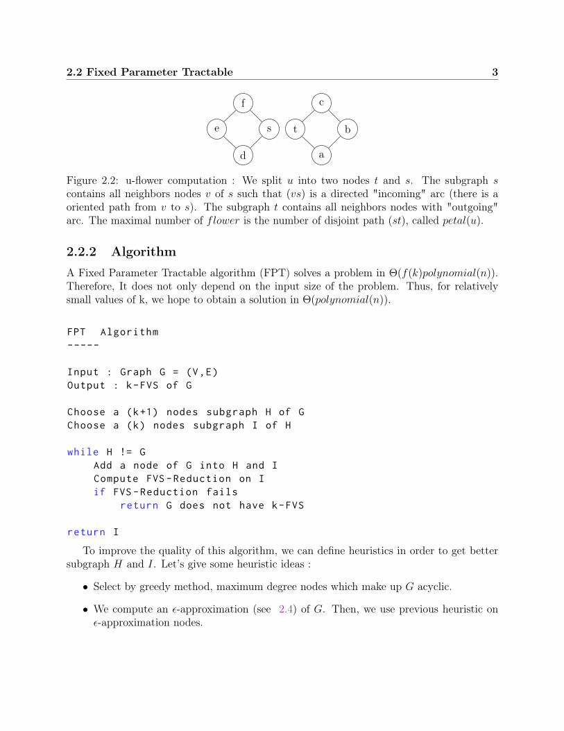
Figure 2.2: u-flower computation : We split u into two nodes t and s. The subgraph scontains all neighbors nodes v of s such that (vs) is a directed "incoming" arc (there is aoriented path from v to s). The subgraph t contains all neighbors nodes with "outgoing"arc. The maximal number of flower is the number of disjoint path (st), called petal(u).

2.2.2 Algorithm

A Fixed Parameter Tractable algorithm (FPT) solves a problem in Θ(f(k)polynomial(n)).Therefore, It does not only depend on the input size of the problem. Thus, for relativelysmall values of k, we hope to obtain a solution in Θ(polynomial(n)).

FPT Algorithm-----

Input : Graph G = (V,E)Output : k-FVS of G

Choose a (k+1) nodes subgraph H of GChoose a (k) nodes subgraph I of H

while H != GAdd a node of G into H and ICompute FVS -Reduction on Iif FVS -Reduction fails

return G does not have k-FVS

return I

To improve the quality of this algorithm, we can define heuristics in order to get bettersubgraph H and I. Let’s give some heuristic ideas :

• Select by greedy method, maximum degree nodes which make up G acyclic.

• We compute an ε-approximation (see 2.4) of G. Then, we use previous heuristic onε-approximation nodes.


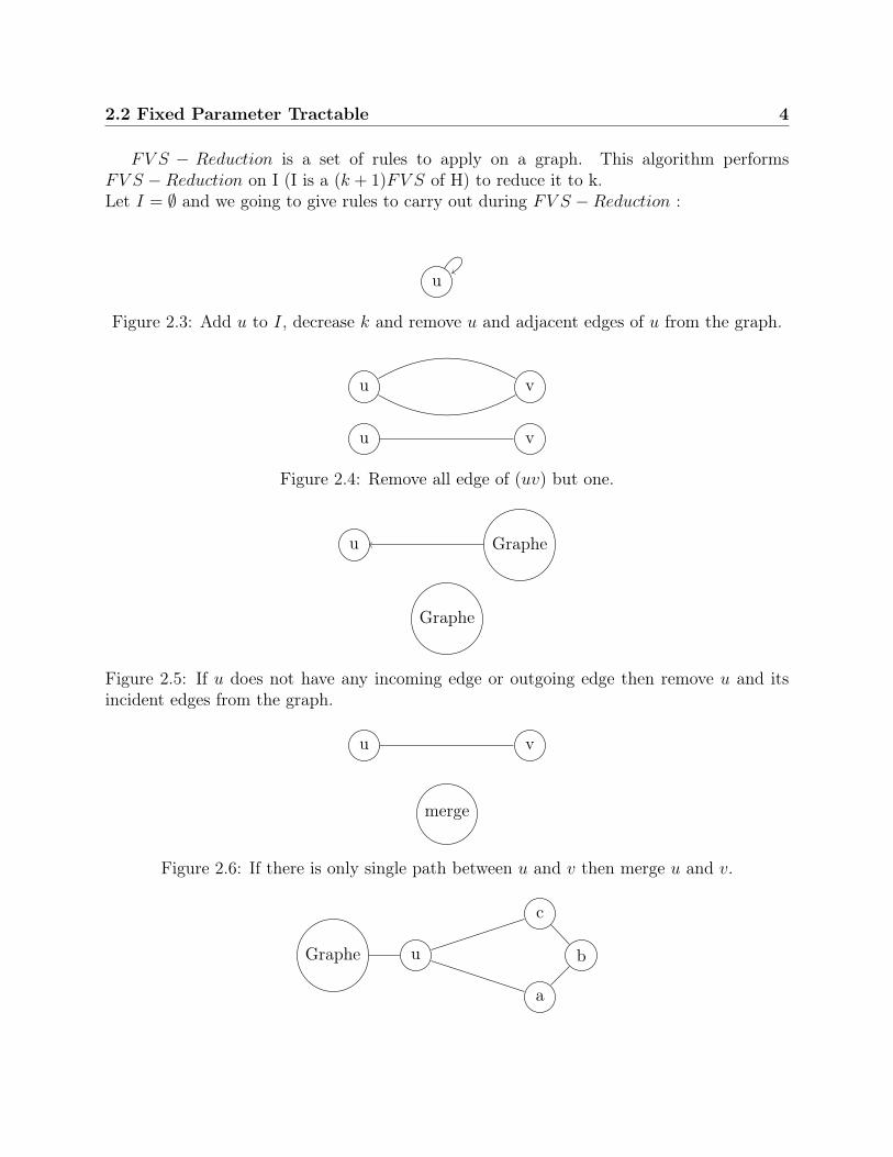
FV S − Reduction is a set of rules to apply on a graph. This algorithm performsFV S −Reduction on I (I is a (k + 1)FV S of H) to reduce it to k.Let I = ∅ and we going to give rules to carry out during FV S −Reduction :

u

Figure 2.3: Add u to I, decrease k and remove u and adjacent edges of u from the graph.

u v

u v

Figure 2.4: Remove all edge of (uv) but one.

u Graphe

Graphe

Figure 2.5: If u does not have any incoming edge or outgoing edge then remove u and itsincident edges from the graph.

u v

merge

Figure 2.6: If there is only single path between u and v then merge u and v.

uGraphe

a

b

c


Graphe

a

b

c

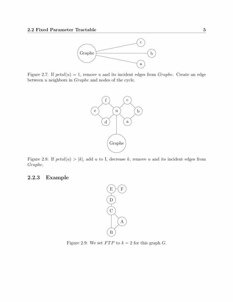
Figure 2.7: If petal(u) = 1, remove u and its incident edges from Graphe. Create an edgebetween u neighbors in Graphe and nodes of the cycle.

u

Graphe

a

b

c

d

e

f

Figure 2.8: If petal(u) > |k|, add u to I, decrease k, remove u and its incident edges fromGraphe.

2.2.3 Example

A

B

C

D

E F

Figure 2.9: We set FTP to k = 2 for this graph G.


A

B

C

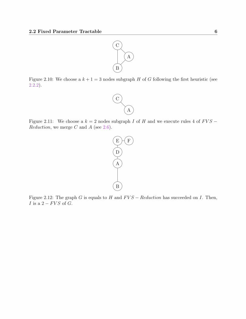
Figure 2.10: We choose a k + 1 = 3 nodes subgraph H of G following the first heuristic (see2.2.2).

A

C

Figure 2.11: We choose a k = 2 nodes subgraph I of H and we execute rules 4 of FV S −Reduction, we merge C and A (see 2.6).

B

A

D

E F

Figure 2.12: The graph G is equals to H and FV S −Reduction has succeeded on I. Then,I is a 2− FV S of G.

2.3 Disjoint-FVS 7

2.3 Disjoint-FVS

2.3.1 Definitions et notations

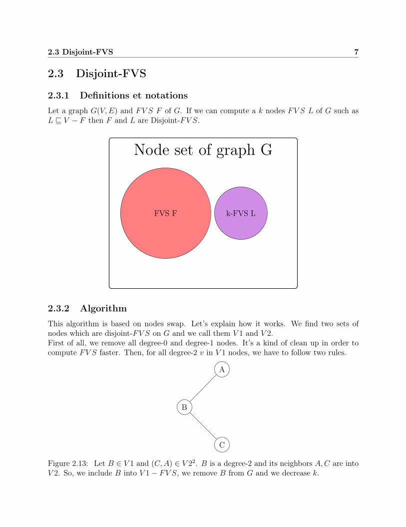
Let a graph G(V,E) and FV S F of G. If we can compute a k nodes FV S L of G such asL v V − F then F and L are Disjoint-FV S.

Node set of graph G

FVS F k-FVS L

2.3.2 Algorithm

This algorithm is based on nodes swap. Let’s explain how it works. We find two sets ofnodes which are disjoint-FV S on G and we call them V 1 and V 2.First of all, we remove all degree-0 and degree-1 nodes. It’s a kind of clean up in order tocompute FV S faster. Then, for all degree-2 v in V 1 nodes, we have to follow two rules.

B

A

C

Figure 2.13: Let B ∈ V 1 and (C,A) ∈ V 22. B is a degree-2 and its neighbors A,C are intoV 2. So, we include B into V 1− FV S, we remove B from G and we decrease k.

2.3 Disjoint-FVS 8

B

A

C

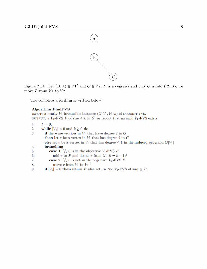
Figure 2.14: Let (B,A) ∈ V 12 and C ∈ V 2. B is a degree-2 and only C is into V 2. So, wemove B from V 1 to V 2.

The complete algorithm is written below :

2.4 2-Approximation 9

2.4 2-Approximation

2.4.1 Definitions and notations

Let the function w : V (G)→ N denotes the weight of a node in the graph G.A graph G is clean if it contains no vertex of degree less than two.A cycle C is semidisjoint if ∀u ∈ C, d(u) = 2 with at most one exception.

2.4.2 Algorithm

An approximation algorithm gives an approximate solution to a complex problem. The qual-ity of an approximation algorithm is given by the ratio r of the solution approached on theoptimal solution.

We will use a 2-approximation algorithm that applies only to weighted and undirected graphs.This algorithm will be based on the principle of local searches. This principle focuses on asubgraph H of G and attempts to resolve the problem on H. Thus, if we can make H acyclicthat means that we can remove cycles on G. This process is repeated until G has no morecycles. The 2-approximation algorithm is bounded by Θ(min|E|log|V |, |V |2).

2.4 2-Approximation 10

2.4.3 Example

A

B

C

D

E F

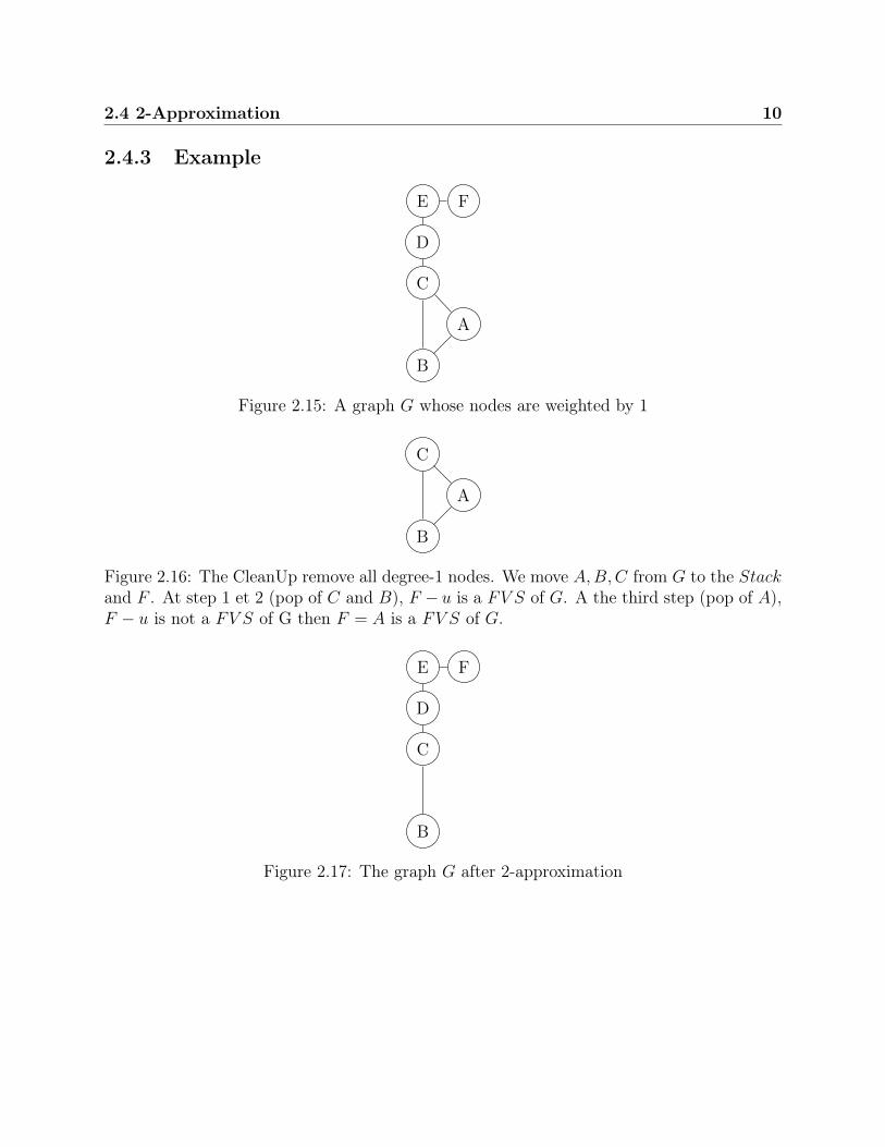
Figure 2.15: A graph G whose nodes are weighted by 1

A

B

C

Figure 2.16: The CleanUp remove all degree-1 nodes. We move A,B,C from G to the Stackand F . At step 1 et 2 (pop of C and B), F − u is a FV S of G. A the third step (pop of A),F − u is not a FV S of G then F = A is a FV S of G.

B

C

D

E F

Figure 2.17: The graph G after 2-approximation

2.5 Randomized Algorithm 11

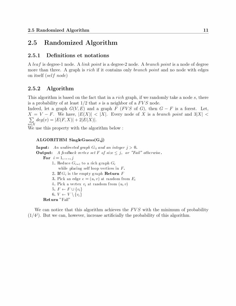
2.5 Randomized Algorithm

2.5.1 Definitions et notations

A leaf is degree-1 node. A link point is a degree-2 node. A branch point is a node of degreemore than three. A graph is rich if it contains only branch point and no node with edgeson itself (self node)

2.5.2 Algorithm

This algorithm is based on the fact that in a rich graph, if we randomly take a node s, thereis a probability of at least 1/2 that s is a neighbor of a FV S node.Indeed, let a graph G(V,E) and a graph F (FV S of G), then G − F is a forest. Let,X = V − F . We have, |E(X)| < |X|. Every node of X is a branch point and 3|X| <∑w∈X

deg(v) = |E(F,X)|+ 2|E(X)|.

We use this property with the algorithm below :

We can notice that this algorithm achieves the FV S with the minimum of probability(1/4j). But we can, however, increase artificially the probability of this algorithm.

2.5 Randomized Algorithm 12

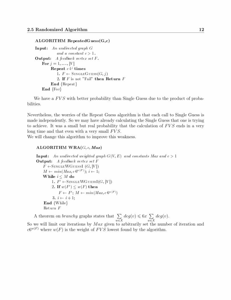
We have a FV S with better probability than Single Guess due to the product of proba-bilities.

Nevertheless, the worries of the Repeat Guess algorithm is that each call to Single Guess ismade independently. So we may have already calculating the Single Guess that one is tryingto achieve. It was a small but real probability that the calculation of FV S ends in a verylong time and that even with a very small FV S.We will change this algorithm to improve this weakness.

A theorem on branchy graphs states that∑w∈X

deg(v) 6 6x∑w∈X

deg(v).

So we will limit our iterations by Max given to arbitrarily set the number of iteration andc6w(F ) where w(F ) is the weight of FV S lowest found by the algorithm.

3. Conclusion

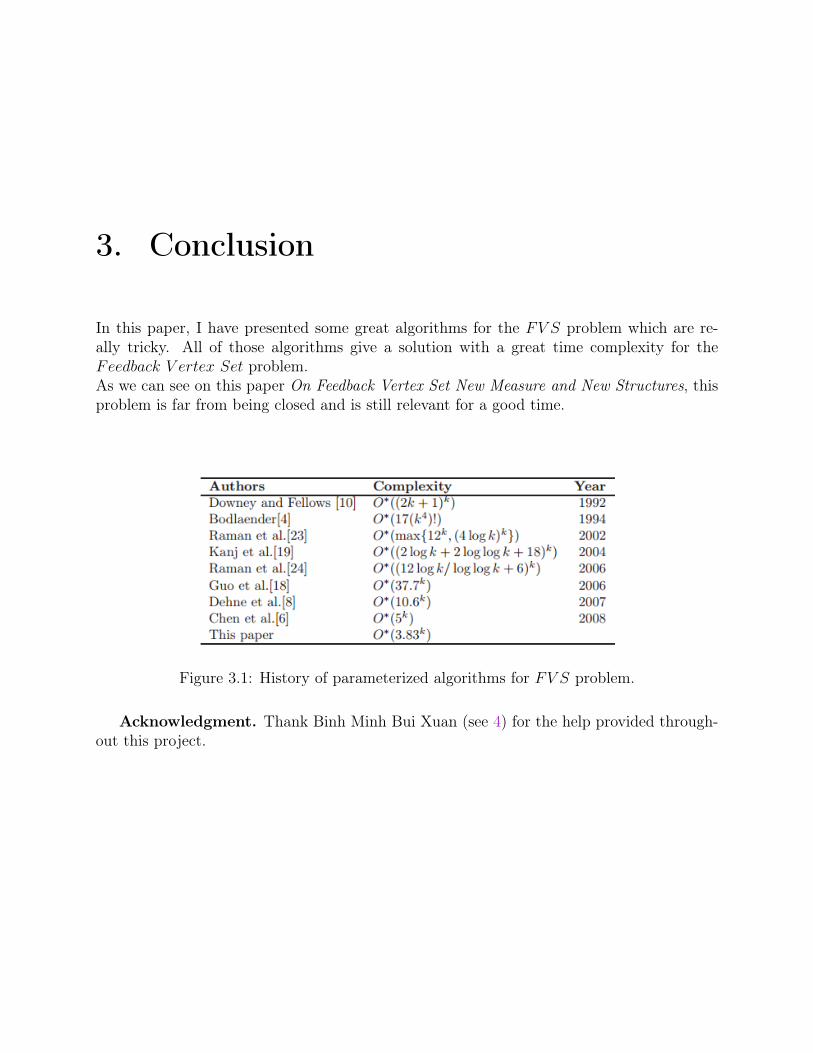
In this paper, I have presented some great algorithms for the FV S problem which are re-ally tricky. All of those algorithms give a solution with a great time complexity for theFeedback V ertex Set problem.As we can see on this paper On Feedback Vertex Set New Measure and New Structures, thisproblem is far from being closed and is still relevant for a good time.

Figure 3.1: History of parameterized algorithms for FV S problem.

Acknowledgment. Thank Binh Minh Bui Xuan (see 4) for the help provided through-out this project.

4. References

• Binh-Minh Bui-Xuan | Algorithms, Programs and Resolution Team, LIP6 | http://www-apr.lip6.fr/ buixuan/

• Irit Dinur, Samuel Safra, On the hardness of approximating vertex cover, 2005 Annalsof Mathematics, Pages 439-485 from Volume 162

• Fedor V. Fomin, Serge Gaspers, Artem V. Pyatkin, Igor Razgon, On the MinimumFeedback Vertex Set Problem: Exact and Enumeration Algorithms, 2007 , Algorith-mica, Volume 52, Issue 2 , pp 293-307

• Igor Razgon , Computing Minimum Directed Feedback Vertex Set in O(1.9977n) , 2007, WSPC

• Jianer Chen, Yang Liu, Songjian Lu, Barry O’sullivan, Igor Razgon , A fixed-parameteralgorithm for the directed feedback vertex set problem , Volume 55 Issue 5, October2008 Article No. 21 , Journal of the ACM (JACM)

• Jianer Chena, Fedor V. Fominb, Yang Liua, Songjian Lua, Yngve Villangerb , Improvedalgorithms for feedback vertex set problems , 2008 , Journal of Computer and SystemSciences, Volume 74, Issue 7

• Ann Becker, Dan Geiger , Optimization of Pearl’s method of conditioning and greedy-like approximation algorithms for the vertex feedback set problem , 1996 , ArtificialIntelligence Volume 83, Issue 1

• Bafna, V., Berman, P., and Fujito, T. (1995). Constant ratio approximations of theweighted feedback vertex set problem for undirected graphs. In Proceedings of theSixth Annual Symposium on Algorithms and Computation (ISAAC95)

• Bar-Yehuda, R., Geiger, D., Naor, J., Roth, R. (1994). Approximation algorithmsfor the feedback vertex set problems with applications to constraint satisfaction andBayesian inference. In Proceedings of the 5th Annual ACM-Siam Symposium OnDiscrete Algorithms, pp. 344,354.

• Fedor V. Fomin Serge Gaspers Artem V. Pyatkin Igor Razgon, On the minimum feed-back vertex set problem : Exact and enumeration algorithms. (2007).

15

• Rudolf Fleischer, Xi Wu, Liwei Yuan, Experimental Study of FPT Algorithms for theDirected Feedback Vertex Set Problem (2009). 17th Annual European Symposium,Copenhagen, Denmark, September 7-9, 2009. Proceedings

• A. Becker, R. Bar-Yehuda and D. Geiger (2000) "Randomized Algorithms for the LoopCutset Problem", Volume 12, pages 219-234

• Yixin Cao, Jianer Chen, Yang Liu, On Feedback Vertex Set: New Measure and NewStructures, Algorithm Theory - SWAT 2010, 12th Scandinavian Symposium and Work-shops on Algorithm Theory, Bergen, Norway, June 21-23, 2010. Proceedings

• Vineet Bafna, Piotr Berman, Toshihiro Fujito, A 2-Approximation Algorithm for theUndirected Feedback Vertex Set Problem, SIAM Journal on Discrete Mathematics,Volume 12 Issue 3, Sept. 1999, Pages 289-297

Software

Feedback Vertex Set