Decision Tree Learning

CSCI-B 659

Decision Trees

Milind Gokhale

February 4, 2015

Decision Tree Learning Agenda

• Decision Tree Representation

• ID3 Learning Algorithm

• Entropy, Information Gain

• An Illustrative Example

• Issues in Decision Tree Learning

CSCI-B 659 | Decision Trees

Decision Tree Learning

• It is a method of approximating discrete-valued functions

that is robust to noisy data and capable of learning

disjunctive expressions

• The learned function is represented by a decision tree.

• Disjunctive Expressions – (A ∧ B ∧ C) ∨ (D ∧ E ∧ F)


Decision Tree Representation

• Each internal node tests an

attribute

• Each branch corresponds to an

attribute value

• Each leaf node assigns a

classification

PlayTennis: This decision tree classifies Saturday mornings

according to whether or not they are suitable for playing tennis


Decision Tree Representation - Classification

• An example is classified by

sorting it through the tree from

the root to the leaf node

• Example – (Outlook = Sunny,

Humidity = High) =>

(PlayTennis = No)

PlayTennis: This decision tree classifies Saturday mornings

according to whether or not they are suitable for playing tennis


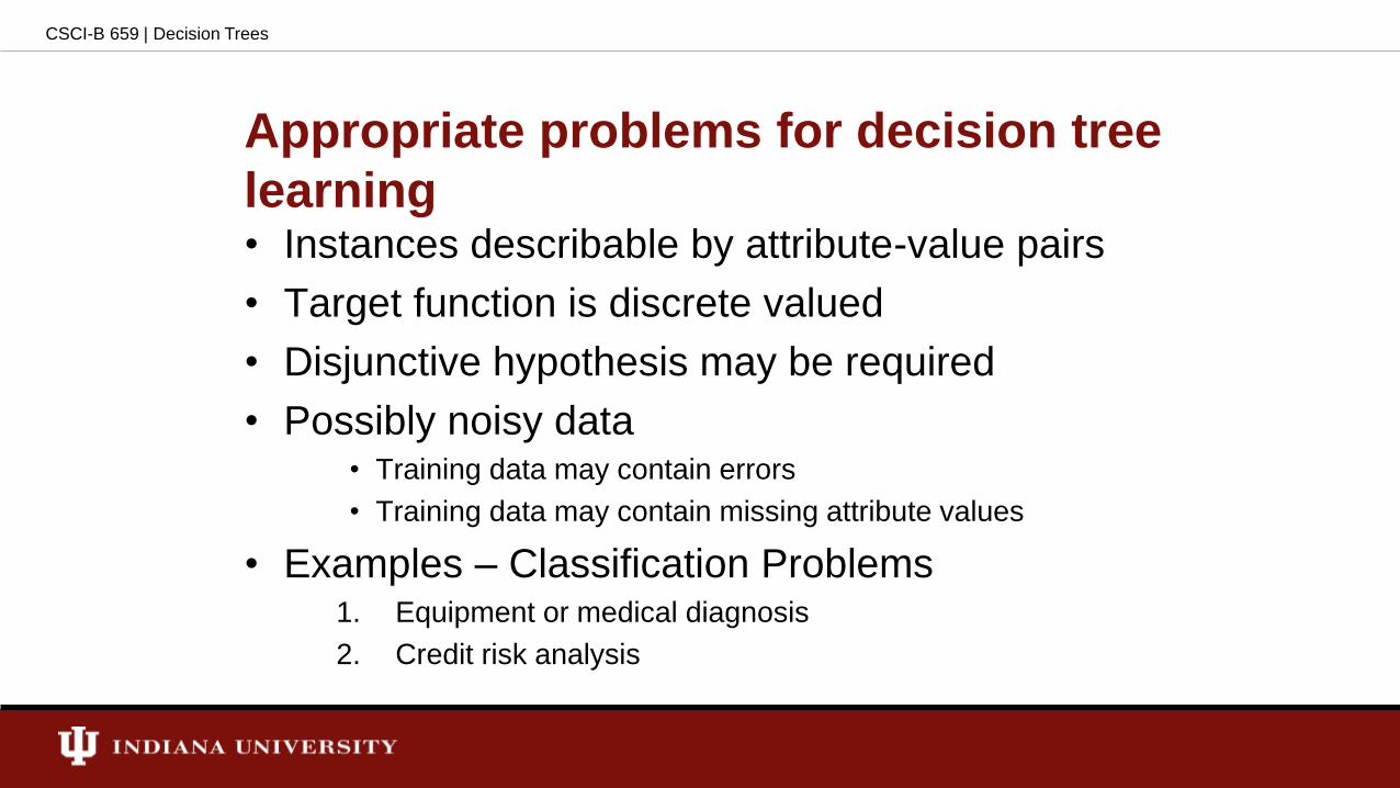
Appropriate problems for decision tree

learning• Instances describable by attribute-value pairs

• Target function is discrete valued

• Disjunctive hypothesis may be required

• Possibly noisy data• Training data may contain errors

• Training data may contain missing attribute values

• Examples – Classification Problems1. Equipment or medical diagnosis

2. Credit risk analysis


Basic ID3 Learning Algorithm approach

• Top-down construction of the tree, beginning with the question "which attribute

should be tested at the root of the tree?'

• Each instance attribute is evaluated using a statistical test to determine how

well it alone classifies the training examples.

• The best attribute is selected and used as the test at the root node of the tree.

• A descendant of the root node is then created for each possible value of this

attribute.

• The training examples are sorted to the appropriate descendant node

• The entire process is then repeated at the descendant node using the training

examples associated with each descendant node

• GREEDY Approach

• No Backtracking - So we may get a suboptimal solution.


ID3 Algorithm


Top-Down induction of decision trees

1. Find A = the best decision attribute for next node

2. Assign A as decision attribute for node

3. For each value of A create new descendants of node

4. Sort the training examples to the leaf node.

5. If training examples classified perfectly, STOP else

iterate over the new leaf nodes.


Which attribute is the best classifier?

• Information Gain – A statistical property that measures

how well a given attribute separates the training

examples according to their target classification.

• This measure is used to select among the candidate

attributes at each step while growing the tree.


Entropy

• S is a sample of training examples

• is the proportion of positive examples in S

• is the proportion of negative examples in S

• Then the entropy measures the impurity of S:

• But If the target attribute can take c different

values:


The entropy varies between 0 and 1.

if all the members belong to the same

class => The entropy = 0

if there are equal number of positive and

negative examples => The entropy = 1

Entropy - Example

• Entropy([29+, 35-]) = - (29/64) log2(29/64) - (35/64) log2(35/64)

= 0.994


Information Gain

• Gain(S,A) = expected reduction in entropy due to sorting

on A

• Here sv is simply the sum of the entropies of each

subset, weighted by the fraction of examples |sv/s| that

belong to sv


Information Gain - Example

• Gain(S,A1)

= 0.994 – (26/64)*.706 – (38/64)*.742

= 0.266

• Information gained by partitioning

along attribute A1 is 0.266


E=0.706 E=0.742

E=0.994 E=0.994

E=0.937 E=0.619

• Gain(S,A2)

= 0.994 – (51/64)*.937 – (13/64)*.619

= 0.121

• Information gained by partitioning

along attribute A2 is 0.121

An Illustrative Example




• Gain(S, Outlook) = 0.246

• Gain(S, Humidity) = 0.151

• Gain(S, Wind) = 0.048

• Gain(S, Temperature) = 0.029

• Since Outlook attribute provides the

best prediction of the target attribute,

PlayTennis, it is selected as the

decision attribute for the root node, and

branches are created with its possible

values (i.e., Sunny, Overcast, and

Rain).



• Ssunny = {D1,D2,D8,D9,D11}

• Gain (Ssunny , Humidity)

= .970 - (3/5) 0.0 - (2/5) 0.0

= .970

• Gain (S sunny , Temperature)

= .970 - (2/5) 0.0 - (2/5) 1.0 - (1/5) 0.0

= .570

• Gain (S sunny , Wind)

= .970 - (2/5) 1.0 - (3/5) .918

= .019

Inductive Bias in ID3

• Inductive bias is the set of assumptions that along with

the training data justify the classifications assigned by

the learner to future instances.

• Given H as the power set of instances X

• ID3 has preference of short trees with high information

gain attributes near the root.

• ID3 has preference for certain hypotheses over others,

with no hard restriction on the hypotheses space H.


Occam’s Razor

• Prefer the simplest hypothesis that fits the data

• Argument in favor -

• A short hypothesis that fits data unlikely to be a coincidence

• A long hypothesis that first data might be a coincidence

• Argument Opposed –

• There are many ways to define small sets of hypotheses

• Two different hypotheses from the same training examples

possible when applied by two learners that perceive these

examples in terms of different internal representations


Issues in Decision Tree Learning

• Overfitting

• Incorporating Continuous-valued attributes

• Attributes with many values

• Handling attributes with costs

• Handling examples with missing attribute values


Overfitting

• Consider a hypothesis h over

• Training data: errortrain(h)

• Entire distribution D of data: errorD(h)

• The hypothesis h ∈ H overfits training data if there is an

alternative hypothesis h’ ∈ H such that

• errortrain(h) < errortrain(h’)

AND

• errorD(h) > errorD(h’)


Overfitting in decision tree learning


Avoiding Overfitting

• Causes

1. This can happen when the training data contains errors or

noise.

2. small numbers of examples are associated with leaf nodes

• Avoiding Overfitting

1. Stop growing when data split not statistically significant

2. Grow full tree, then post-prune it.

• Selecting Best Tree

1. Measure performance over training data

2. Measure performance over separate validation data


Reduced-Error Pruning

• Split data into training and validation sets

• Do until further pruning is harmful

1. Evaluate impact of pruning each possible node on

validation set

2. Greedily remove the one that most improves the validation

set accuracy


Effect of Reduced-Error Pruning


Rule Post-Pruning

• The major drawback of Reduced-Error Pruning is when

the data is limited, validation set reduces even further

the number of examples for training.

Hence Rule Post-Pruning

• Convert tree to equivalent set of rules

• Prune each rule independently of others

• Sort final rules into desired sequence for use


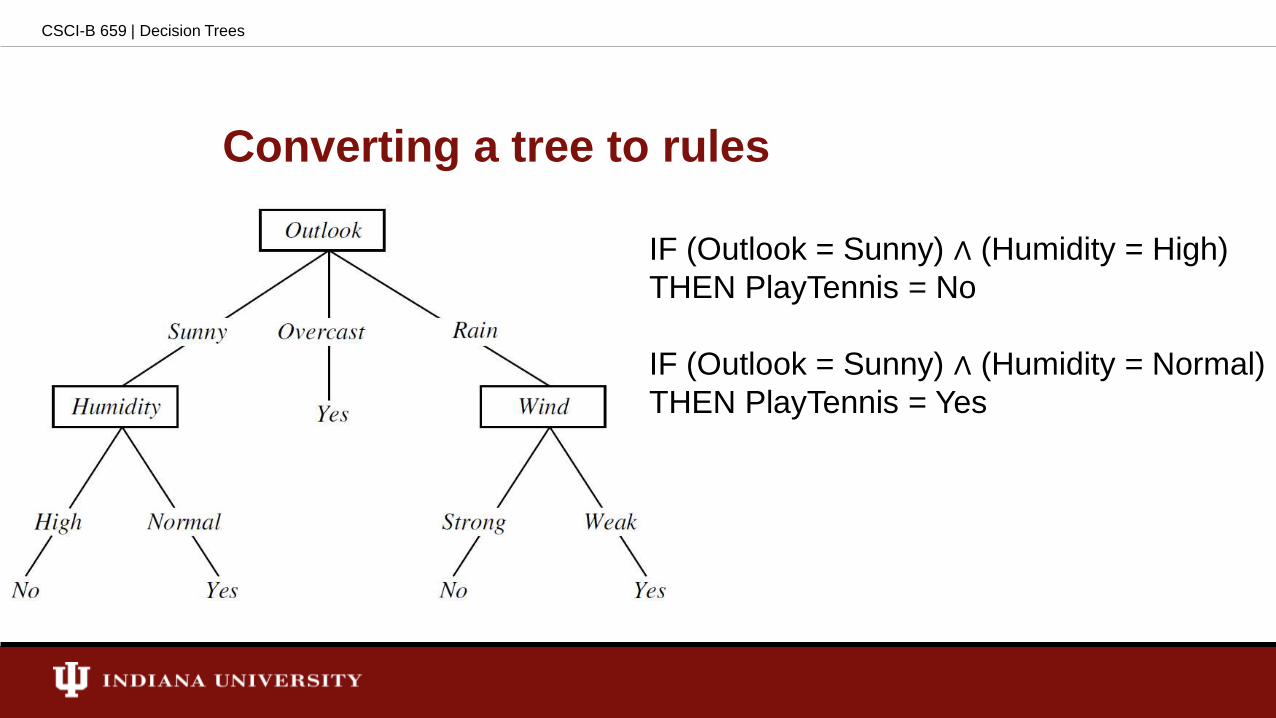
Converting a tree to rules


IF (Outlook = Sunny) ∧ (Humidity = High)

THEN PlayTennis = No

IF (Outlook = Sunny) ∧ (Humidity = Normal)

THEN PlayTennis = Yes

Continuous Valued-Attributes

• Create a discrete-valued attribute to test continuous

• So if Temperature = 75

• We can infer that PlayTennis = Yes


Attributes with many values

• Problem:

• If attribute has many values, Gain will select any value

• Example – Using date attribute

• One approach – Gain Ratio

Where si is a subset of S which has value vi


Attributes with costs

• Problem:

• Medical diagnosis, BloodTest has cost $150

• Robotics, Width_from_1ft has cost 23 sec

• One Approach - replace gain

• Tan and Schlimmer (1990)

• Nunez (1988)

• where w ∈ [0, 1] is a constant that determines the relative importance of cost versus information

gain.


Examples with missing attribute values

• What if some examples missing values of attribute A?

• Use training examples anyway and sort through tree

• If node n tests A, Assign it the most common value among

the examples at node n

• Assign a probability pi to each possible value of A – vi and

assign fraction pi of example to each descendant in tree


Some of the latest Applications


Gesture Recognition

Motion Detection

Xbox 360 Kinect

Thank You


References

• Mitchell, Tom M. "Decision Tree Learning." In Machine

Learning. New York: McGraw-Hill, 1997.

• Flach, Peter A. "Tree Models: Decision Trees."

In Machine Learning: The Art and Science of Algorithms

That Make Sense of Data. Cambridge: Cambridge

University Press, 2012.


Software

Decision Tree Learning