Wavelets & Wavelet Algorithms: Longitudinal Waves, Sinusoids, & Fourier's Discovery

Wavelets & Wavelet Algorithms

Vladimir Kulyukin

www.vkedco.blogspot.comwww.vkedco.blogspot.com

Longitudinal Waves, Sinusoids, &

Fourier's Discovery

http://www.linkedin.com/pub/vladimir-kulyukin/23/2a2/150

http://www.vkedco.blogspot.com/

Outline

● Longitudinal Waves● Overview of Fourier's Analysis● Sinusoids● Programmatic Manipulation of Sinusoids in

Octave/Matlab● Sinusoid Synthesis

Longitudinal Waves

Signal Waves

● Sound transmits through a medium such as a gas or a liquid

● Transmission of sound through a medium is conceptualized as longitudinal waves

● Longitudinal waves are caused by alternating pressure deviations (up or down) from the equilibrium pressure

● Light & heat can also be analyzed in terms of waves

Longitudinal Waves

● Ideal longitudinal waves can be viewed as a time series of medium compression (peaks) and decompression (valleys)

● Such series are mathematically represented with sinusoids

Ideal vs Real Waves

● Ideal wavelets are abstract mathematical models of real phenomena

● Waves generated by real phenomena (speech, bee buzzing, etc) are not as regular as their ideal counterparts because they consist of multiple waves and noises

Ideal Wave Real Wave

Spherical Compression of Longitudinal Waves

Click on or go to the link below to watch an animation of spherical compression http://en.wikipedia.org/wiki/Sound#/media/File:Spherical_pressure_waves.gif

http://en.wikipedia.org/wiki/Sound#/media/File:Spherical_pressure_waves.gif

Stationary Floating LeavesIf you drop a pebble into the water and watch a leaf floating on the concentric waves, you will notice that the leaf will not change its position

Sourcehttp://fineartamerica.com/featured/green-leaf-with-water-reflection-sandra-cunningham.html

http://fineartamerica.com/featured/green-leaf-with-water-reflection-sandra-cunningham.html

Floating Leaf's Amplitude vs Time

water level

leaf amplitude

Time

Overview of Fourier's Analysis

Fourier's Discovery

Complex waves can be effectively decomposed into simple waves

Jean-Baptiste Joseph Fourier (1768 - 1830)

Decomposition of Complex Waves

Complex Wave

Simple Wave 1

Simple Wave 2

Simple Wave 3

Steps of Fourier's Analysis: Step 01: Take Complex Wave

Steps of Fourier's Analysis: Step 02: Decompose Wave into Its Constituents ttx 5sin

ttx 4sin2

ttx 3sin3

Steps of Fourier's Analysis: Step 03: Compute Frequency Spectrum ttx 5sin

ttx 4sin2

ttx 3sin3

Elements of Fourier's Analysis

● Sinusoids● Synthesis & Analysis of Synusoids● Tangents & Integrals● Orthogonality of Functions

Sinusoids

Period of a Function

...32

...32

period. a also is ,, then period, a is If

.

such that constant a is thereif periodic is function A

TxfTxfTxfxf

TxfTxfTxfxf

ZkkTT

Txfxf

Txf

Definition

(radians). phase ousinstantane theis

(radians); phase initial theis

(Hz);frequency theis

(sec); timeis

(rad/sec);frequency radian theis

amplitude;peak negative-non theis

constants. are ,, variable;realt independenan is

.sin:form theoffunction a is sinusoidA

t

f

t

A

At

tAtx

Definition

Reference: J. O. Smith III, Mathematics of the Discrete Fourier Transform with Audio Applications, 2nd Edition (https://ccrma.stanford.edu/~jos/st/).

https://ccrma.stanford.edu/~jos/st/

Period of a Sinusoid

value.same thehasfunction thebefore passmust

that timeofamount theis period the:period a oftion interpreta Practical

sec.2

secradrad 2

:secondsin measured are Periods

.2

period itsThen .sin If

.such that ) called

(sometimes constant a is thereif periodic is function a that Recall

PtAtx

PxfxfT

Pxf

Period of a Sinusoid

.sin2sin

2sin

2

.2

is sin of period that theShow

txtAtA

tAtxPtx

tAtxP

Frequency

Hz2sec 2sec

211

time.of units 2every hasfunction periodic a

thatnsoscillatio ofnumber theis Frequency

P

f

f

What is an Oscillation?

time.of units

second) 1 e.g., measure,other some(or 2 into packed be

can graphssuch many how indicates frequency Thus,

period. complete

one ofgraph theasn oscillatio one ofcan think You

f

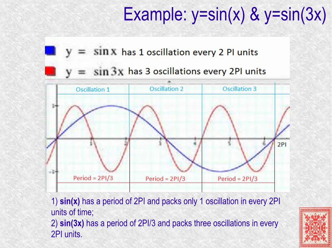
Example: y=sin(x) & y=sin(3x)

1) sin(x) has a period of 2PI and packs only 1 oscillation in every 2PI units of time;2) sin(3x) has a period of 2PI/3 and packs three oscillations in every 2PI units.

Phase

.sin0 ,0 then when,sin If

axis.- on theoffset theas of thought becan Phase

AxttAtx

y

Phase: Example 01

second.every valuesits repeats Thus,

sec. 1

secrad

2

rad 2

secradrad 2

Then .sec

rad 2 Suppose

.sinLet

tx

P

tAtx

Phase: Example 02

seconds. 2every valuesits repeats Thus,

sec. 2

secrad

1

rad 2

secradrad 2

Then .sec

rad 1 Suppose

.sinLet

tx

P

tAtx

Phase: Example 03


sec. 4

secrad

5.0

rad 2

secradrad 2

Then .sec

rad 5.0 Suppose

.sinLet

tx

P

tAtx

Phase: Example 04


sec. 8

secrad

25.0

rad 2

secradrad 2

Then .sec

rad 25.0 Suppose

.sinLet

tx

P

tAtx

Phase: Example 05

seconds. 0.5every valuesits repeats Thus,

sec. 5.0

secrad

4

rad 2

secradrad 2

Then .sec

rad 4 Suppose

.sinLet

tx

P

tAtx

Phase: Example 06

seconds. 0.25every valuesits repeats Thus,

sec. 25.0

secrad

8

rad 2

secradrad 2

Then .sec

rad 8 Suppose

.sinLet

tx

P

tAtx

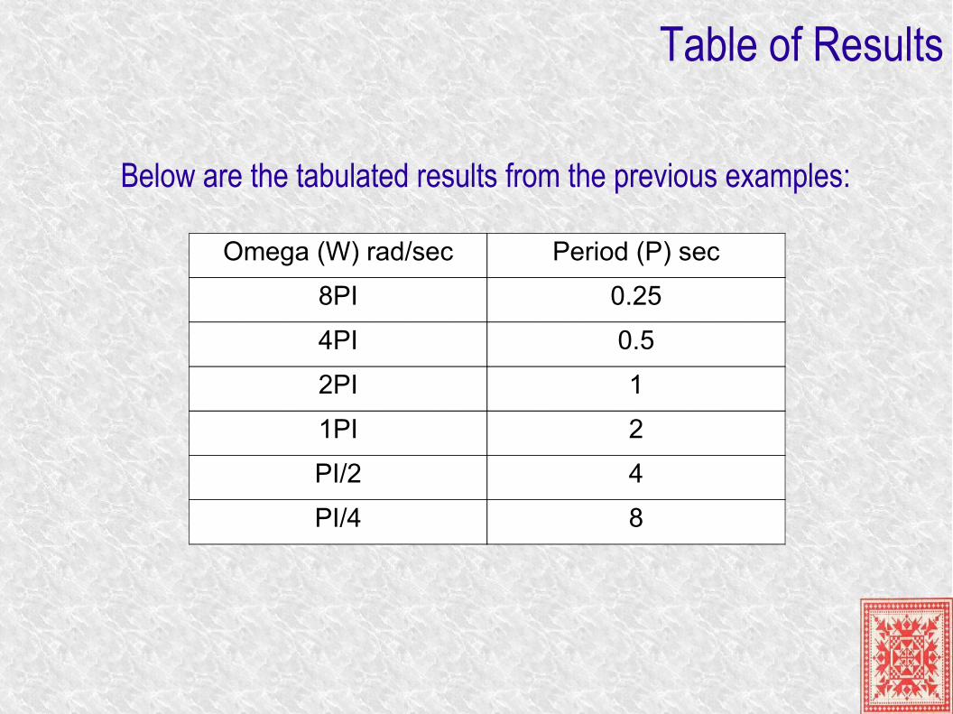
Table of Results

Omega (W) rad/sec Period (P) sec

8PI 0.25

4PI 0.5

2PI 1

1PI 2

PI/2 4

PI/4 8

Below are the tabulated results from the previous examples:

Observation: Rotational Velocity & Period

versa. viceand position, same the

reach point to theit takeslonger theorigin,an around rotatespoint a

slower that theconclude we velocity,rotational a as of think weIf

seconds.in of valuelonger the the,rad/secin set smaller we The

P

Obtaining Sinusoids from y(t)=sin(t)

.by each valuemultiply 4)

; 1by axis- thealong curve shift the 3)

axis);-( axis- thealong xpandcompress/e 2)

; 2 as of period thecompute 1)

:follows as

sin from onbtained becan sin sinusoidAny

A

t

xt

ty

ttxtAty

Graph Interpretation of Sinusoid Periods

axis). (time axis- the

along expand graph will theThus, slower).repeat will valuesthe

(i.e.,longer is period its hence slower, rotatespoint the, 1 If

axis). (time axis- thealong compress graph will the

Thus, faster).repeat will values the(i.e.,shorter be willperiod its

hence faster, rotatespoint the, 1 If .2 of period a has sin

x

x

t

seconds. 8

412

is of period theand sec

rad

4

1Then .

4

1sin and sinLet

seconds. 3

2is of period theand

sec

rad 3Then .3sin and sinLet

tyttyttx

tyttyttx

Example: y=sin(x) & y=sin(3x)

sin(3x) exhibits a uniform contraction along the x-axis by a factor of 3.

Rotational Velocity & Frequency

Rotational Velocity: Example 01

time.of units 2

containing intervalan in times0.5 oscillates Thus,

Hz.5.0sec 2

11

sec. 2

secrad

1

rad 2

secradrad 2

.sec

rad 1 Suppose

.sinLet

txP

f

P

tAtx


sec. 01.0

ofduration a has sample each taken Thus, sec. 01.011

sample? each taken of )(duration time theisWhat

c.samples/se 100 take that wemeans This .sec

1100Hz100 that Suppose

ss

s

fT

Tf

T

f


time.of units 2every n oscillatio 1 has Thus,

Hz 1sec 1

11

sec. 1

secrad

2

rad 2

secradrad 2

.sec

rad 2 Suppose

.sinLet

txP

f

P

tAtx


time.of units 2every nsoscillatio 2 has Thus,

Hz. 2sec 5.0

11

sec. 5.0

secrad

4

rad 2

secradrad 2

Then .sec

rad 4 Suppose

.sinLet

tx

Pf

P

tAtx



Hz 4sec 25.0

11

sec. 25.0

secrad

8

rad 2

secradrad 2

.sec

rad 8 Suppose

.sinLet

tx

Pf

P

tAtx


time.of units 2every nsoscillatio 0.25 has Thus,

Hz. 25.0sec 4

11

sec. 4

secrad

5.0

rad 2

secradrad 2

Then .sec

rad 5.0 Suppose

.sinLet

tx

Pf

P

tAtx



Hz. 125.0sec 8

11

sec. 8

secrad

25.0

rad 2

secradrad 2

Then .sec

rad 25.0 Suppose

.sinLet

tx

Pf

P

tAtx



Hz. 0625.0sec 16

11

sec. 16

secrad

125.0

rad 2

secradrad 2

Then .sec

rad 125.0 Suppose

.sinLet

tx

Pf

P

tAtx



Hz.2

3

sec3

211

sec.3

2

secrad

3

rad 2

secradrad 2

So .sec

rad 3Then

.3sinLet

tx

Pf

P

ttx

Observation: Rotational Velocity & Frequency

versa. viceand time,of units 2every hasit

nsoscillatiofewer theorigin, thearound rotatespoint aslower the

that concludecan then we velocity,rotational a as of think weIf

.frequency esmaller th the, velocity rotational esmaller th The

f

Rotational Velocity & Frequency

Click on or go to the link below to watch an animation of sinusoids & circles http://en.wikipedia.org/wiki/Sine_wave#/media/File:ComplexSinInATimeAxe.gif

http://en.wikipedia.org/wiki/Sine_wave#/media/File:ComplexSinInATimeAxe.gif

Programmatic Sinusoid Manipulation in

Octave/Matlab

Sinusoids, Circles, & Phases

Octave on Ubuntu

The above screenshot is taken on my Ubuntu 12.04 LTS command line. It shows command line interaction with Octave.

Sinusoids in Octave/Matlab

phi = 0; %% phase offsett = 0:0.001:1; %% time x-axisw = 2*pi; %% angular frequencyang=0:0.01:2*pi; %% angle array for drawing circles

%% sine curvessin01 = 1*sin(5*w*t+phi); %% sin curve 01; f = 5, amp = 1sin02 = 2*sin(4*w*t+phi); %% sin curve 02; f = 4, amp = 2sin03 = 3*sin(3*w*t+phi); %% sin curve 03; f = 3, amp = 3sin04 = 4*sin(2*w*t+phi); %% sin curve 04; f = 2, amp = 4sin05 = 5*sin(1*w*t+phi); %% sin curve 05; f = 1, amp = 5

Zero Phase Sinusoids

Sinusoid ttx 5sin

%% plot of sinusoid 01figure;plot(t, sin01);xlabel('Time (s)');ylabel('Amplitude');title('1*sin(5*w*t)');

%% circle 01figure;x1=0;y1=0;r1=1; xp1=r1*cos(ang);yp1=r1*sin(ang);plot(x1+xp1,y1+yp1);hold on;plot([0,r1*cos(phi)], [0, r1*sin(phi)]);title(strcat('Circle with r=1, phi=', num2str(phi)));

phi = 0; t = 0:0.001:1; w = 2*pi; ang = 0:0.01:2*pi; %% sine curvessin01 = 1*sin(5*w*t+phi); sin02 = 2*sin(4*w*t+phi); sin03 = 3*sin(3*w*t+phi); sin04 = 4*sin(2*w*t+phi); sin05 = 5*sin(1*w*t+phi);

Sinusoid ttx 4sin2

%% ********* SINUSOID 02 PLOTS ***********%% 2*sin(4*w*t+phi)%% plot of sinusoid 02

figure;plot(t, sin02);xlabel('Time (s)')ylabel('Amplitude')title('2*sin(4*w*t)')


phi = 0; t = 0:0.001:1; w = 2*pi; ang = 0:0.01:2*pi; %% sine curvessin01 = 1*sin(5*w*t+phi); sin02 = 2*sin(4*w*t+phi); sin03 = 3*sin(3*w*t+phi); sin04 = 4*sin(2*w*t+phi); sin05 = 5*sin(1*w*t+phi);

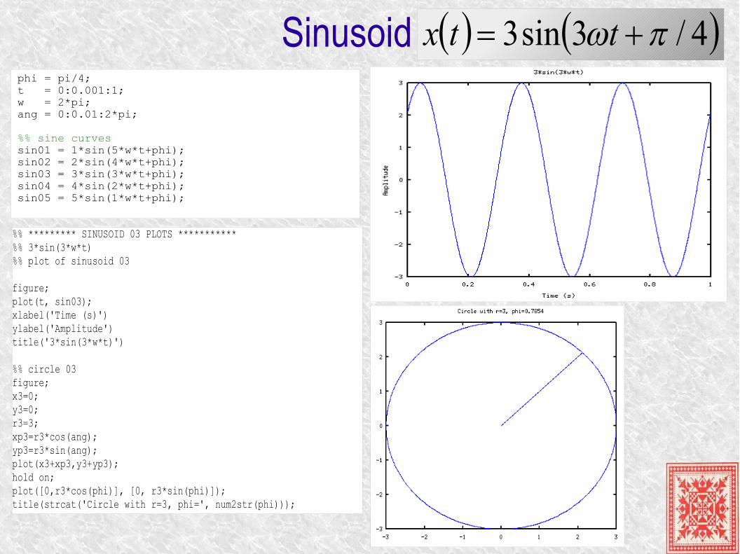
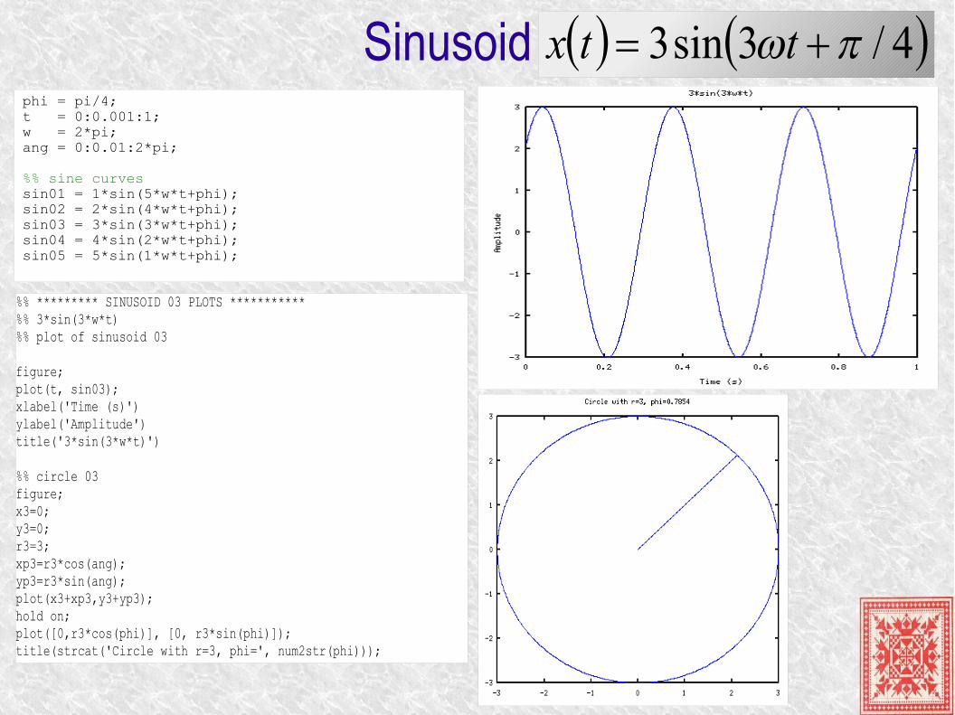
Sinusoid ttx 3sin3

%% ********* SINUSOID 03 PLOTS ***********%% 3*sin(3*w*t)%% plot of sinusoid 03


%% circle 03figure;x3=0;y3=0;r3=3;xp3=r3*cos(ang);yp3=r3*sin(ang);plot(x3+xp3,y3+yp3);hold on;plot([0,r3*cos(phi)], [0, r3*sin(phi)]);title(strcat('Circle with r=3, phi=', num2str(phi)));

Sinusoid ttx 2sin4

%% ********* SINUSOID 04 PLOTS ***********%% 4*sin(2*w*t)%% plot of sinusoid 04figure;plot(t, sin04);xlabel('Time (s)');ylabel('Amplitude');title('4*sin(2*w*t)');


Sinusoid ttx 1sin5

%% ********* SINUSOID 05 PLOTS ***********%% sin05 = 5*sin(1*w*t)figure;plot(t, sin05);xlabel('Time (s)');ylabel('Amplitude');title('5*sin(1*w*t)');


Sinusoids with Phase = Pi/4

Sinusoid 4/5sin ttx

%% plot of sinusoid 01figure;plot(t, sin01);xlabel('Time (s)');ylabel('Amplitude');title('1*sin(5*w*t)');


phi = pi/4; t = 0:0.001:1; w = 2*pi; ang = 0:0.01:2*pi; %% sine curvessin01 = 1*sin(5*w*t+phi); sin02 = 2*sin(4*w*t+phi); sin03 = 3*sin(3*w*t+phi); sin04 = 4*sin(2*w*t+phi); sin05 = 5*sin(1*w*t+phi);

Sinusoid

%% ********* SINUSOID 02 PLOTS ***********%% 2*sin(4*w*t+phi)%% plot of sinusoid 02



4/4sin2 ttxphi = pi/4; t = 0:0.001:1; w = 2*pi; ang = 0:0.01:2*pi; %% sine curvessin01 = 1*sin(5*w*t+phi); sin02 = 2*sin(4*w*t+phi); sin03 = 3*sin(3*w*t+phi); sin04 = 4*sin(2*w*t+phi); sin05 = 5*sin(1*w*t+phi);

Sinusoid 4/3sin3 ttx











%% ********* SINUSOID 04 PLOTS ***********%% 4*sin(2*w*t)%% plot of sinusoid 04figure;plot(t, sin04);xlabel('Time (s)');ylabel('Amplitude');title('4*sin(2*w*t)');




%% ********* SINUSOID 05 PLOTS ***********%% sin05 = 5*sin(1*w*t)figure;plot(t, sin05);xlabel('Time (s)');ylabel('Amplitude');title('5*sin(1*w*t)');



Sine & Cosine CurvesSide by Side

Sine & Cosine Curves

ttx 5sin ttx 5cos


ttx 3sin3 ttx 3cos3


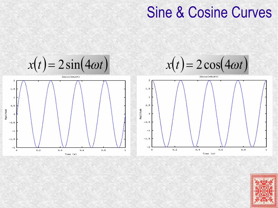
ttx 4sin2 ttx 4cos2


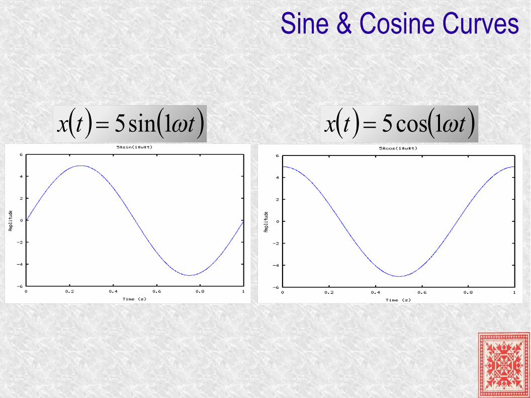
ttx 1sin5 ttx 1cos5


ttx 2sin4 ttx 2cos4

Sinusoid Synthesis

Function Synthesis & Analysis● Like numbers, new functions can be obtained

(synthesized) from existing functions via addition, subtraction, multiplication, and division

● All these function operations are pointwise: in other words, the values of functions at specific points are added, subtracted, multiplied, or divided (division by 0 is still not allowed!)

● To analyze a complex function is to obtain the list of functions and function operations through which the complex function was synthesized

phi = 0; %% phase offset; defaults to 0, try it with pi/2, pi/4, pi/10, etc. t = 0:0.001:1; %% time x-axisw = 2*pi; %% angular frequencyang = 0:0.01:2*pi; %% angle array for drawing circles %% sine curvessin01 = 1*sin(5*w*t+phi); %% sin curve 01; f = 5, amp = 1sin02 = 2*sin(4*w*t+phi); %% sin curve 02; f = 4, amp = 2sin03 = 3*sin(3*w*t+phi); %% sin curve 03; f = 3, amp = 3sin04 = 4*sin(2*w*t+phi); %% sin curve 04; f = 2, amp = 4sin05 = 5*sin(1*w*t+phi); %% sin curve 05; f = 1, amp = 5 %% cosine curvescos01 = 1*cos(5*w*t+phi); %% cos curve 01; f = 5, amp = 1cos02 = 2*cos(4*w*t+phi); %% cos curve 02; f = 4, amp = 2cos03 = 3*cos(3*w*t+phi); %% cos curve 03; f = 3, amp = 3cos04 = 4*cos(2*w*t+phi); %% cos curve 04; f = 2, amp = 4cos05 = 5*cos(1*w*t+phi); %% cos curve 05; f = 1, amp = 5 %% combined sinusoidscsin01 = sin01 + sin02;csin02 = sin01 + sin02 + sin03;csin03 = sin01 + cos01;csin04 = sin02 + cos03 + cos05; %% ===== COMBINED SINUSOIDS %% ****** plot of csin01=sin01+sin02figure;plot(t, csin01);xlabel('Time (s)')ylabel('Amplitude')title('1*sin(5*w*t)+2*sin(4*w*t+phi)')

Curve Synthesis: Example 01


ttx 4sin2

ttx 5sin1

+

phi = 0; %% phase offset; defaults to 0, try it with pi/2, pi/4, pi/10, etc. t = 0:0.001:1; %% time x-axisw = 2*pi; %% angular frequencyang = 0:0.01:2*pi; %% angle array for drawing circles %% sine curvessin01 = 1*sin(5*w*t+phi); %% sin curve 01; f = 5, amp = 1sin02 = 2*sin(4*w*t+phi); %% sin curve 02; f = 4, amp = 2sin03 = 3*sin(3*w*t+phi); %% sin curve 03; f = 3, amp = 3sin04 = 4*sin(2*w*t+phi); %% sin curve 04; f = 2, amp = 4sin05 = 5*sin(1*w*t+phi); %% sin curve 05; f = 1, amp = 5 %% cosine curvescos01 = 1*cos(5*w*t+phi); %% cos curve 01; f = 5, amp = 1cos02 = 2*cos(4*w*t+phi); %% cos curve 02; f = 4, amp = 2cos03 = 3*cos(3*w*t+phi); %% cos curve 03; f = 3, amp = 3cos04 = 4*cos(2*w*t+phi); %% cos curve 04; f = 2, amp = 4cos05 = 5*cos(1*w*t+phi); %% cos curve 05; f = 1, amp = 5 %% combined sinusoidscsin01 = sin01 + sin02;csin02 = sin01 + sin02 + sin03;csin03 = sin01 + cos01;csin04 = sin02 + cos03 + cos05; %% ===== COMBINED SINUSOIDS %% ******* plot of csin02=sin01+sin02+sin03figure;plot(t, csin02);xlabel('Time (s)');ylabel('Amplitude');title('1*sin(5*w*t)+2*sin(4*w*t+phi)+3*sin(3*w*t+phi)');



+

ttx 5sin1

ttx 4sin2

ttx 3sin3

phi = 0; %% phase offset; defaults to 0, try it with pi/2, pi/4, pi/10, etc. t = 0:0.001:1; %% time x-axisw = 2*pi; %% angular frequencyang = 0:0.01:2*pi; %% angle array for drawing circles %% sine curvessin01 = 1*sin(5*w*t+phi); %% sin curve 01; f = 5, amp = 1sin02 = 2*sin(4*w*t+phi); %% sin curve 02; f = 4, amp = 2sin03 = 3*sin(3*w*t+phi); %% sin curve 03; f = 3, amp = 3sin04 = 4*sin(2*w*t+phi); %% sin curve 04; f = 2, amp = 4sin05 = 5*sin(1*w*t+phi); %% sin curve 05; f = 1, amp = 5 %% cosine curvescos01 = 1*cos(5*w*t+phi); %% cos curve 01; f = 5, amp = 1cos02 = 2*cos(4*w*t+phi); %% cos curve 02; f = 4, amp = 2cos03 = 3*cos(3*w*t+phi); %% cos curve 03; f = 3, amp = 3cos04 = 4*cos(2*w*t+phi); %% cos curve 04; f = 2, amp = 4cos05 = 5*cos(1*w*t+phi); %% cos curve 05; f = 1, amp = 5 %% combined sinusoidscsin01 = sin01 + sin02;csin02 = sin01 + sin02 + sin03;csin03 = sin01 + cos01;csin04 = sin02 + cos03 + cos05; %% ===== COMBINED SINUSOIDS %% ******* plot of csin03=sin01+cos01figure;plot(t, csin03);xlabel('Time (s)');ylabel('Amplitude');title('1*sin(5*w*t)+1*cos(5*w*t)');



+

ttx 5sin1

ttx 5cos1

phi = 0; %% phase offset; defaults to 0, try it with pi/2, pi/4, pi/10, etc. t = 0:0.001:1; %% time x-axisw = 2*pi; %% angular frequencyang = 0:0.01:2*pi; %% angle array for drawing circles %% sine curvessin01 = 1*sin(5*w*t+phi); %% sin curve 01; f = 5, amp = 1sin02 = 2*sin(4*w*t+phi); %% sin curve 02; f = 4, amp = 2sin03 = 3*sin(3*w*t+phi); %% sin curve 03; f = 3, amp = 3sin04 = 4*sin(2*w*t+phi); %% sin curve 04; f = 2, amp = 4sin05 = 5*sin(1*w*t+phi); %% sin curve 05; f = 1, amp = 5 %% cosine curvescos01 = 1*cos(5*w*t+phi); %% cos curve 01; f = 5, amp = 1cos02 = 2*cos(4*w*t+phi); %% cos curve 02; f = 4, amp = 2cos03 = 3*cos(3*w*t+phi); %% cos curve 03; f = 3, amp = 3cos04 = 4*cos(2*w*t+phi); %% cos curve 04; f = 2, amp = 4cos05 = 5*cos(1*w*t+phi); %% cos curve 05; f = 1, amp = 5 %% combined sinusoidscsin01 = sin01 + sin02;csin02 = sin01 + sin02 + sin03;csin03 = sin01 + cos01;csin04 = sin02 + cos03 + cos05; %% ===== COMBINED SINUSOIDS %% ******* plot of csin04=sin02+cos03+cos05figure;plot(t, csin04);xlabel('Time (s)');ylabel('Amplitude');title('2*sin(4*w*t+phi)+3*cos(3*w*t+phi)+5*cos(1*w*t+phi)');


Curve Synthesis: Example 04 ttx 4sin2

ttx 3cos3

ttx 1cos5

+

References● J. O. Smith III, Mathematics of the Discrete Fourier Transform with

Audio Applications, 2nd Edition.

● G. P. Tolstov. Fourier Series.

Science

Wavelets & Wavelet Algorithms: Longitudinal Waves, Sinusoids, & Fourier's Discovery