Soil moisture spatio-temporal variability: insights from mechanistic ecohydrological

modeling

Simone Fatichi

Institute of Environmental Engineering, ETH Zurich, Zurich, Switzerland simone.fatichi@ifu.baug.ethz.ch

24 September 2015 Padova, Italy

Introduction Methods Results Conclusions

MOTIVATION

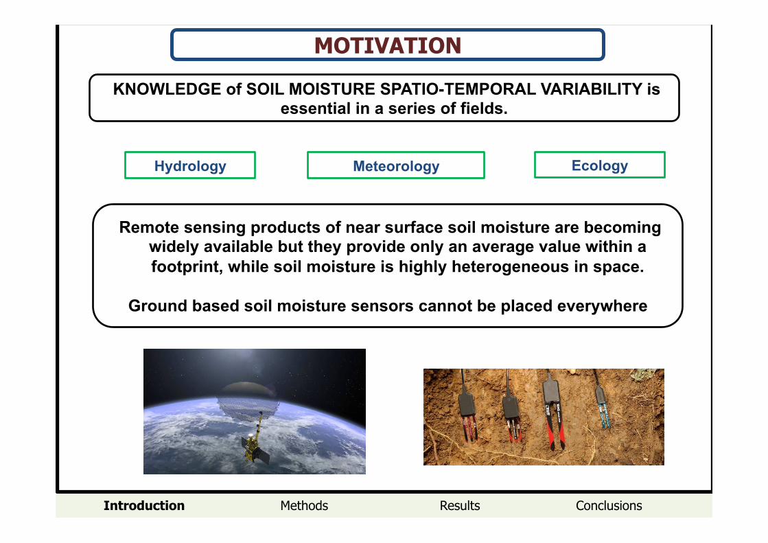
KNOWLEDGE of SOIL MOISTURE SPATIO-TEMPORAL VARIABILITY is essential in a series of fields.

Remote sensing products of near surface soil moisture are becoming widely available but they provide only an average value within a footprint, while soil moisture is highly heterogeneous in space.

Ground based soil moisture sensors cannot be placed everywhere

Ecology Meteorology Hydrology

Introduction Methods Results Conclusions

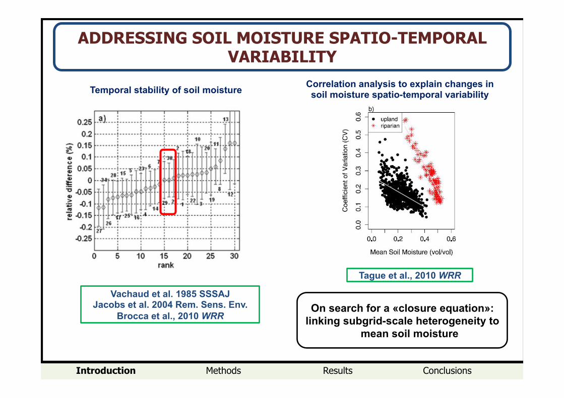
ADDRESSING SOIL MOISTURE SPATIO-TEMPORAL VARIABILITY

Tague et al., 2010 WRR

Vachaud et al. 1985 SSSAJ Jacobs et al. 2004 Rem. Sens. Env.

Brocca et al., 2010 WRR

Temporal stability of soil moisture Correlation analysis to explain changes in soil moisture spatio-temporal variability

On search for a «closure equation»: linking subgrid-scale heterogeneity to

mean soil moisture

Introduction Methods Results Conclusions

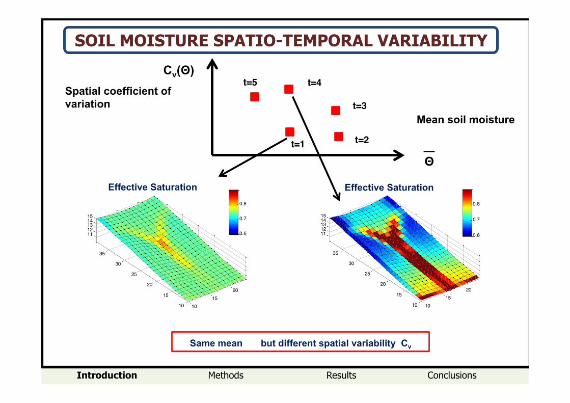
SOIL MOISTURE SPATIO-TEMPORAL VARIABILITY

1015

20

10

15

20

25

30

35

1112131415

Effective Saturation

0.6

0.7

0.8

1015

20

10

15

20

25

30

35

1112131415

Effective Saturation

0.6

0.7

0.8

Same mean "  but different spatial variability Cv

Θ

Cv(Θ)

Effective Saturation Effective Saturation

t=1 t=2

t=3Spatial coefficient of variation!

t=4t=5

Mean soil moisture!

Introduction Methods Results Conclusions

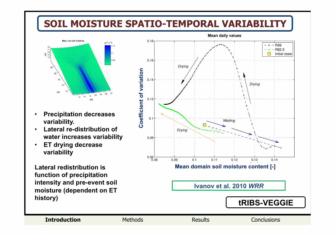
Ivanov et al. 2010 WRR

SOIL MOISTURE SPATIO-TEMPORAL VARIABILITY

•  Precipitation decreases

variability. •  Lateral re-distribution of

water increases variability •  ET drying decrease

variability

Lateral redistribution is function of precipitation intensity and pre-event soil moisture (dependent on ET history)

Mean domain soil moisture content [-]

Coe

ffici

ent o

f var

iatio

n

tRIBS-VEGGIE

Introduction Methods Results Conclusions

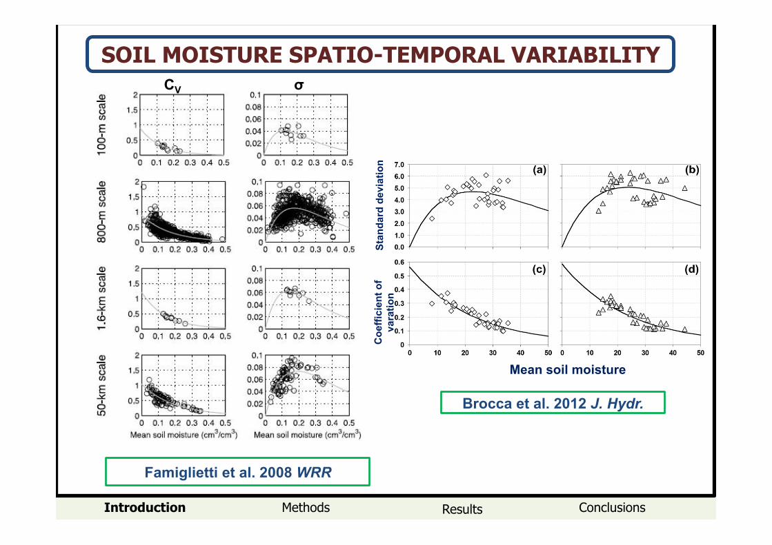
SOIL MOISTURE SPATIO-TEMPORAL VARIABILITY

Famiglietti et al. 2008 WRR

Brocca et al. 2012 J. Hydr.

CV! σ!

Mean soil moisture C

oeffi

cien

t of

vara

tion

Stan

dard

dev

iatio

n

Introduction Methods Results Conclusions

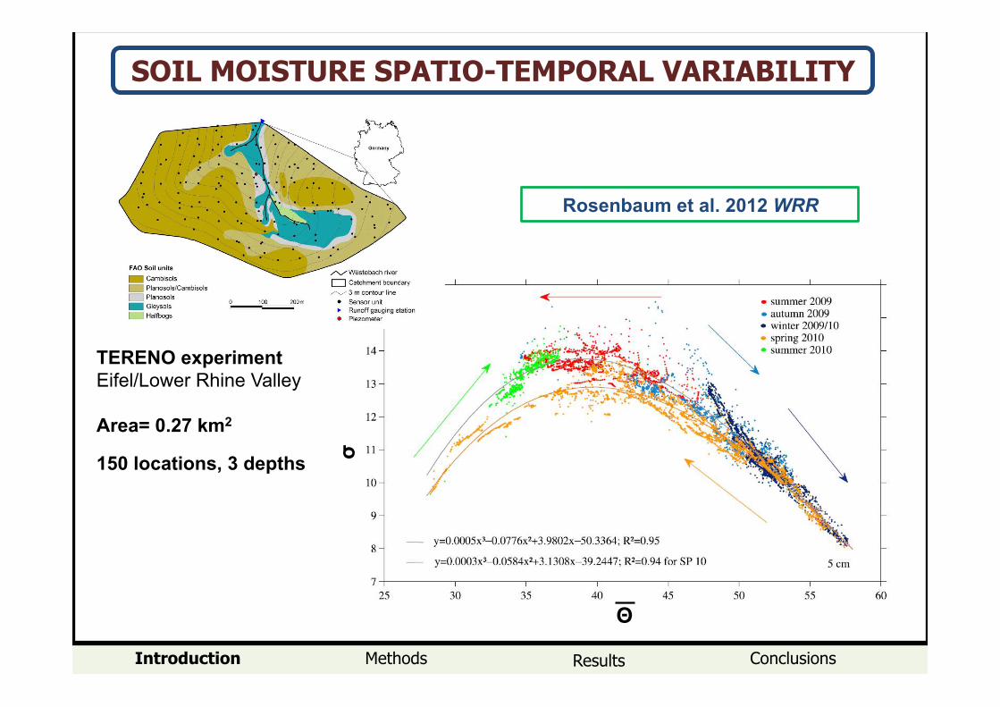
SOIL MOISTURE SPATIO-TEMPORAL VARIABILITY

Rosenbaum et al. 2012 WRR

σ !

Θ

TERENO experiment Eifel/Lower Rhine Valley Area= 0.27 km2

150 locations, 3 depths

Introduction Methods Results Conclusions

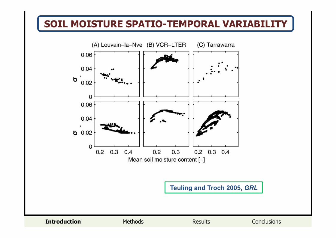
SOIL MOISTURE SPATIO-TEMPORAL VARIABILITY

Teuling and Troch 2005, GRL

σ!σ!

Introduction Methods Results Conclusions

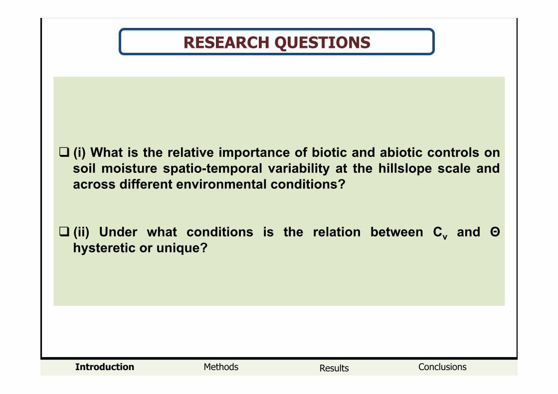
RESEARCH QUESTIONS

! (i) What is the relative importance of biotic and abiotic controls on soil moisture spatio-temporal variability at the hillslope scale and across different environmental conditions?

! (ii) Under what conditions is the relation between Cv and Θ hysteretic or unique?

Introduction Methods Results Conclusions

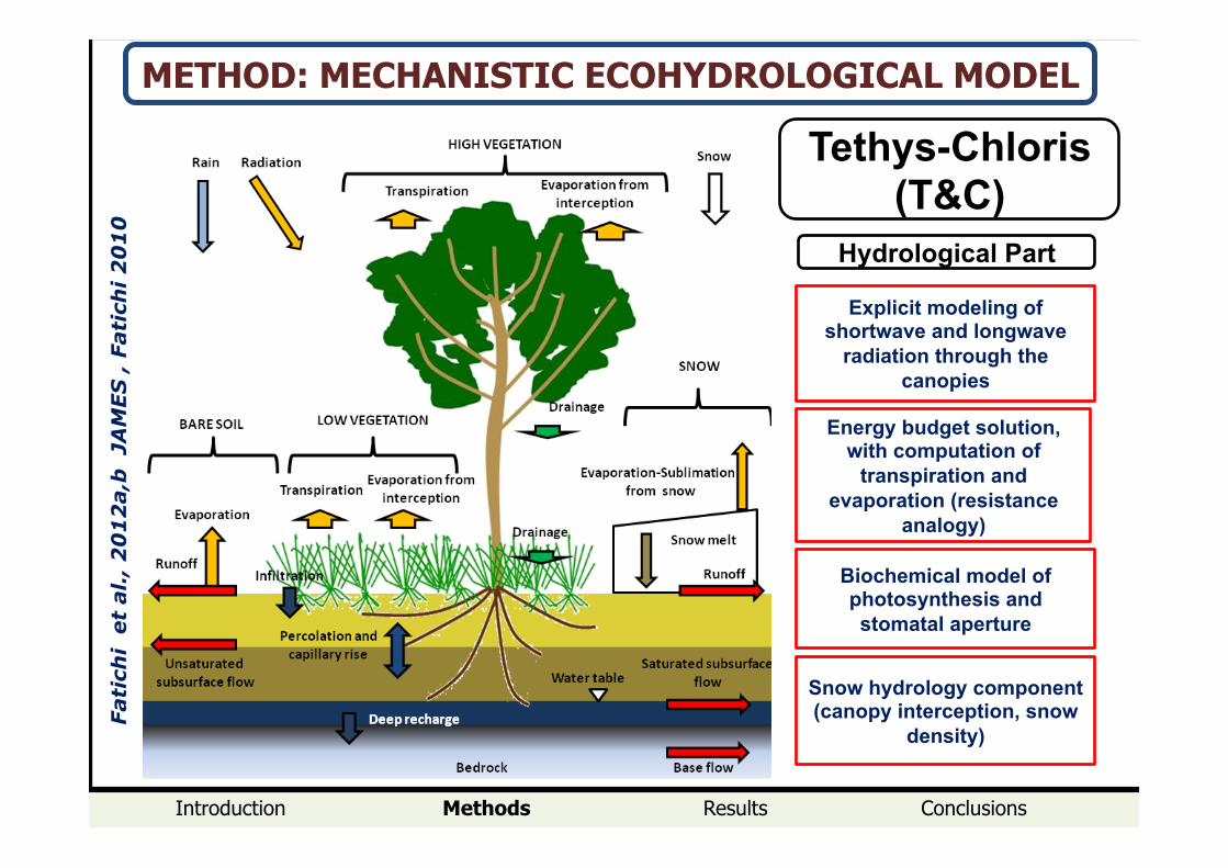
METHOD: MECHANISTIC ECOHYDROLOGICAL MODEL

Tethys-Chloris (T&C)

Explicit modeling of shortwave and longwave

radiation through the canopies

Energy budget solution, with computation of

transpiration and evaporation (resistance

analogy)

Hydrological Part

Biochemical model of photosynthesis and stomatal aperture

Fati

chi

et a

l.,

20

12

a,b

JA

MES

, F

atic

hi 2

01

0

Snow hydrology component (canopy interception, snow

density)

Introduction Methods Results Conclusions

20

4060

80100

120

140160

180

0

20

40

60

80

100

120

140

160

180

300

400

500

600

700

800

900

1000

1100

1200

1300

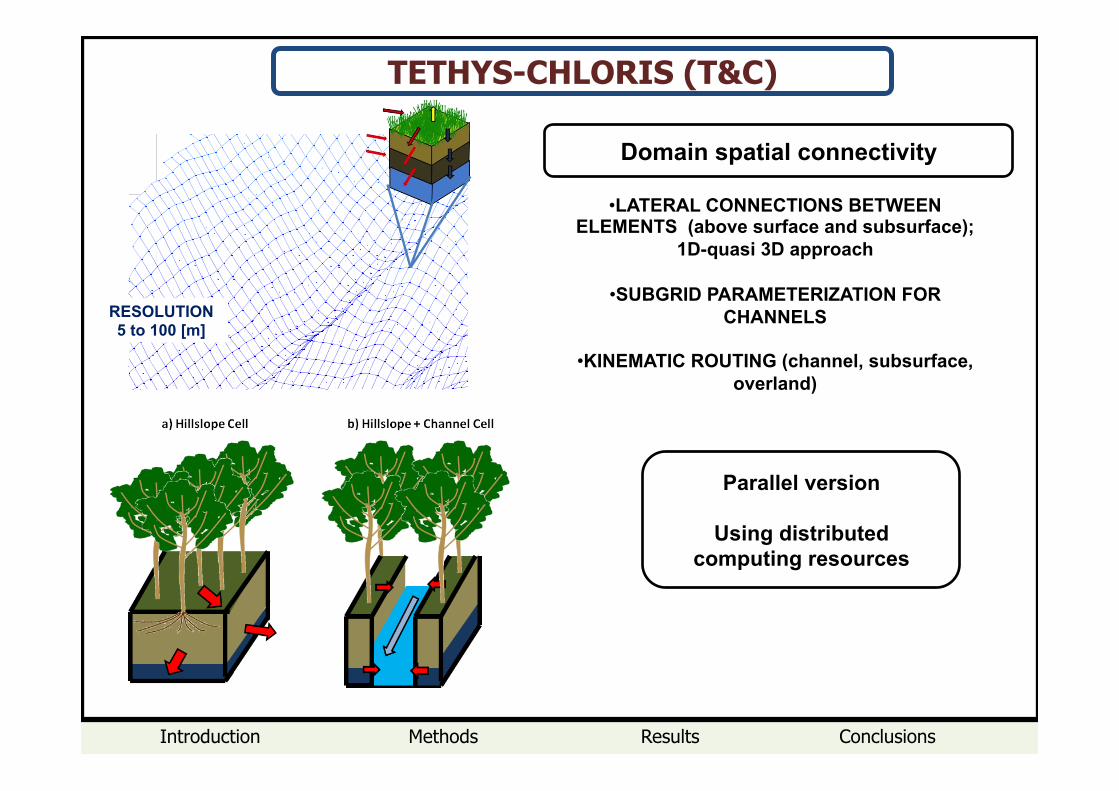
Domain spatial connectivity

RESOLUTION 5 to 100 [m]

• LATERAL CONNECTIONS BETWEEN ELEMENTS (above surface and subsurface);

1D-quasi 3D approach

• SUBGRID PARAMETERIZATION FOR CHANNELS

• KINEMATIC ROUTING (channel, subsurface, overland)

TETHYS-CHLORIS (T&C)

Parallel version

Using distributed computing resources

Introduction Methods Results Conclusions

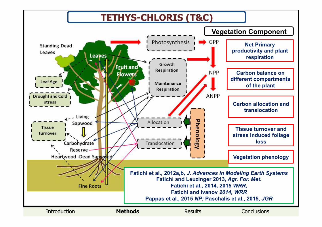
Net Primary productivity and plant

respiration

Carbon allocation and translocation

Tissue turnover and stress induced foliage

loss

Carbon balance on different compartments

of the plant

Vegetation Component

Vegetation phenology

TETHYS-CHLORIS (T&C)

Fatichi et al., 2012a,b, J. Advances in Modeling Earth Systems Fatichi and Leuzinger 2013, Agr. For. Met.

Fatichi et al., 2014, 2015 WRR, Fatichi and Ivanov 2014, WRR

Pappas et al., 2015 NP; Paschalis et al., 2015, JGR

Introduction Methods Results Conclusions

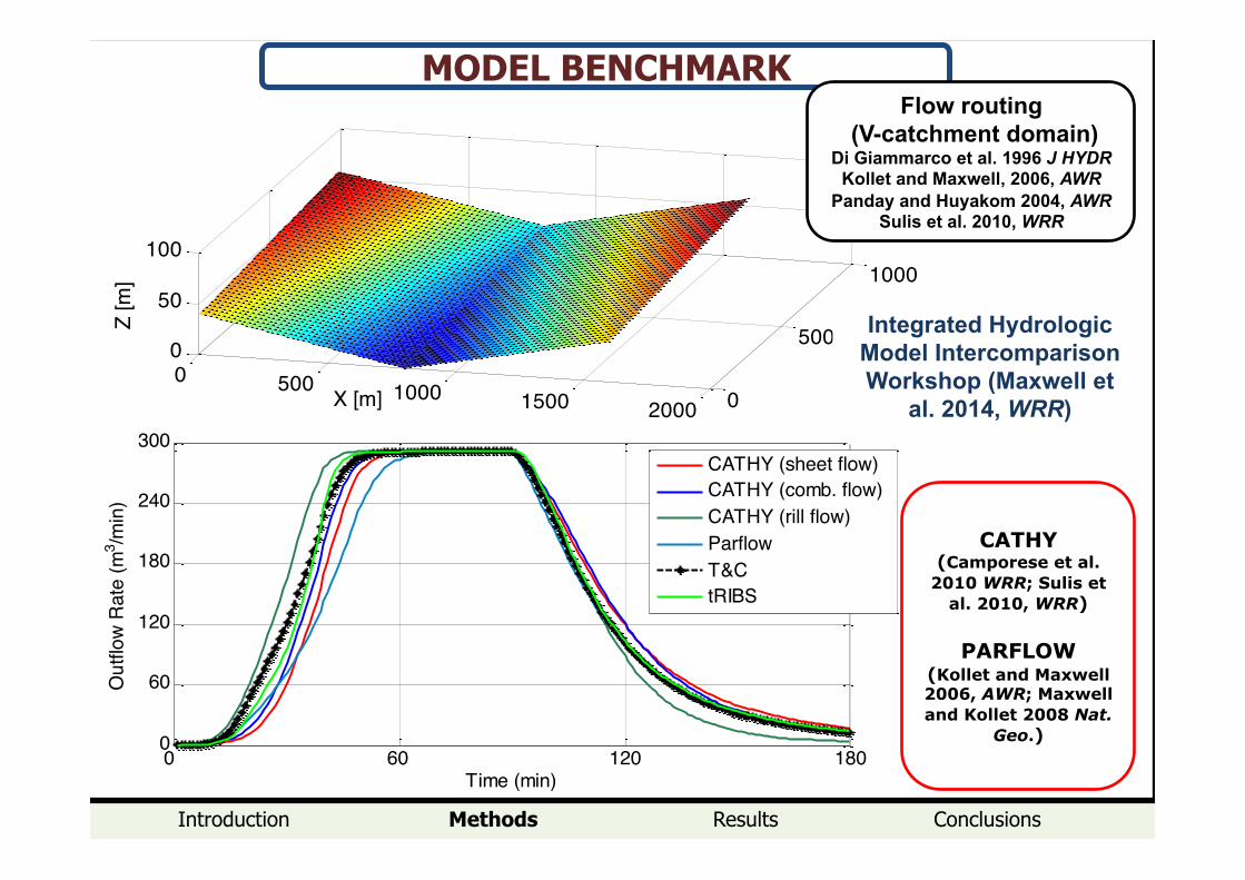
MODEL BENCHMARK

0 60 120 1800

60

120

180

240

300

Time (min)

Out

flow

Rate

(m3 /m

in)

CATHY (sheet flow)CATHY (comb. flow)CATHY (rill flow)ParflowT&CtRIBS

0 500 1000 1500 2000 0

500

1000

0

50

100

Y [m]

X [m]

Z [m

]Flow routing

(V-catchment domain) Di Giammarco et al. 1996 J HYDR

Kollet and Maxwell, 2006, AWR Panday and Huyakom 2004, AWR

Sulis et al. 2010, WRR

CATHY (Camporese et al.

2010 WRR; Sulis et al. 2010, WRR)

PARFLOW

(Kollet and Maxwell 2006, AWR; Maxwell and Kollet 2008 Nat.

Geo.)

Integrated Hydrologic Model Intercomparison Workshop (Maxwell et

al. 2014, WRR)

Introduction Methods Results Conclusions

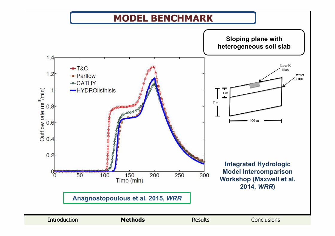
MODEL BENCHMARK

Integrated Hydrologic Model Intercomparison

Workshop (Maxwell et al. 2014, WRR)

Anagnostopoulous et al. 2015, WRR

Sloping plane with heterogeneous soil slab

Introduction Methods Results Conclusions

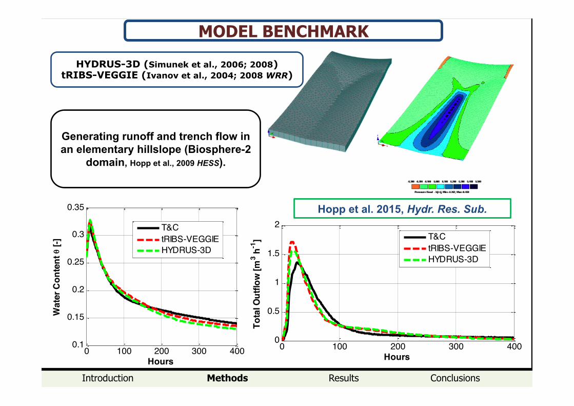
MODEL BENCHMARK

Generating runoff and trench flow in an elementary hillslope (Biosphere-2

domain, Hopp et al., 2009 HESS).

HYDRUS-3D (Simunek et al., 2006; 2008) tRIBS-VEGGIE (Ivanov et al., 2004; 2008 WRR)

0 100 200 300 4000.1

0.15

0.2

0.25

0.3

0.35

Wat

er C

onte

nt θ

[-]

Hours

T&CtRIBS-VEGGIEHYDRUS-3D

0 100 200 300 4000

0.5

1

1.5

2

Tota

l Out

flow

[m3 h

-1]

Hours

T&CtRIBS-VEGGIEHYDRUS-3D

Hopp et al. 2015, Hydr. Res. Sub.

Introduction Methods Results Conclusions

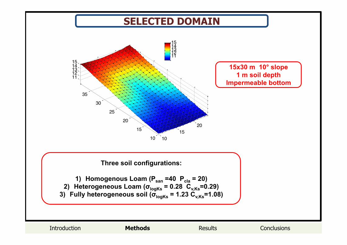
SELECTED DOMAIN

1015

20

10

15

20

25

30

35

1112131415

1112131415

15x30 m 10° slope 1 m soil depth

Impermeable bottom

Three soil configurations:

1)  Homogenous Loam (Psan =40 Pcla = 20) 2)  Heterogeneous Loam (σlogKs = 0.28 Cv,Ks=0.29)

3)  Fully heterogeneous soil (σlogKs = 1.23 Cv,Ks=1.08)

Introduction Methods Results Conclusions

-150 -100 -50 0 50 100 150

-80

-60

-40

-20

0

20

40

60

80

500

1000

1500

2000

2500

3000

3500

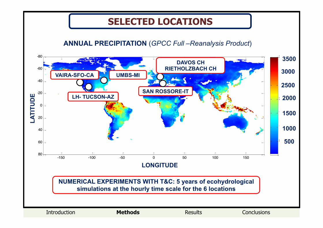
SELECTED LOCATIONS

ANNUAL PRECIPITATION (GPCC Full –Reanalysis Product)

3500

2000

1500

1000

500

VAIRA-SFO-CA UMBS-MI

LH- TUCSON-AZ

DAVOS CH RIETHOLZBACH CH

LONGITUDE

LATI

TUD

E

3000

2500 SAN ROSSORE-IT

NUMERICAL EXPERIMENTS WITH T&C: 5 years of ecohydrological simulations at the hourly time scale for the 6 locations

Introduction Methods Results Conclusions

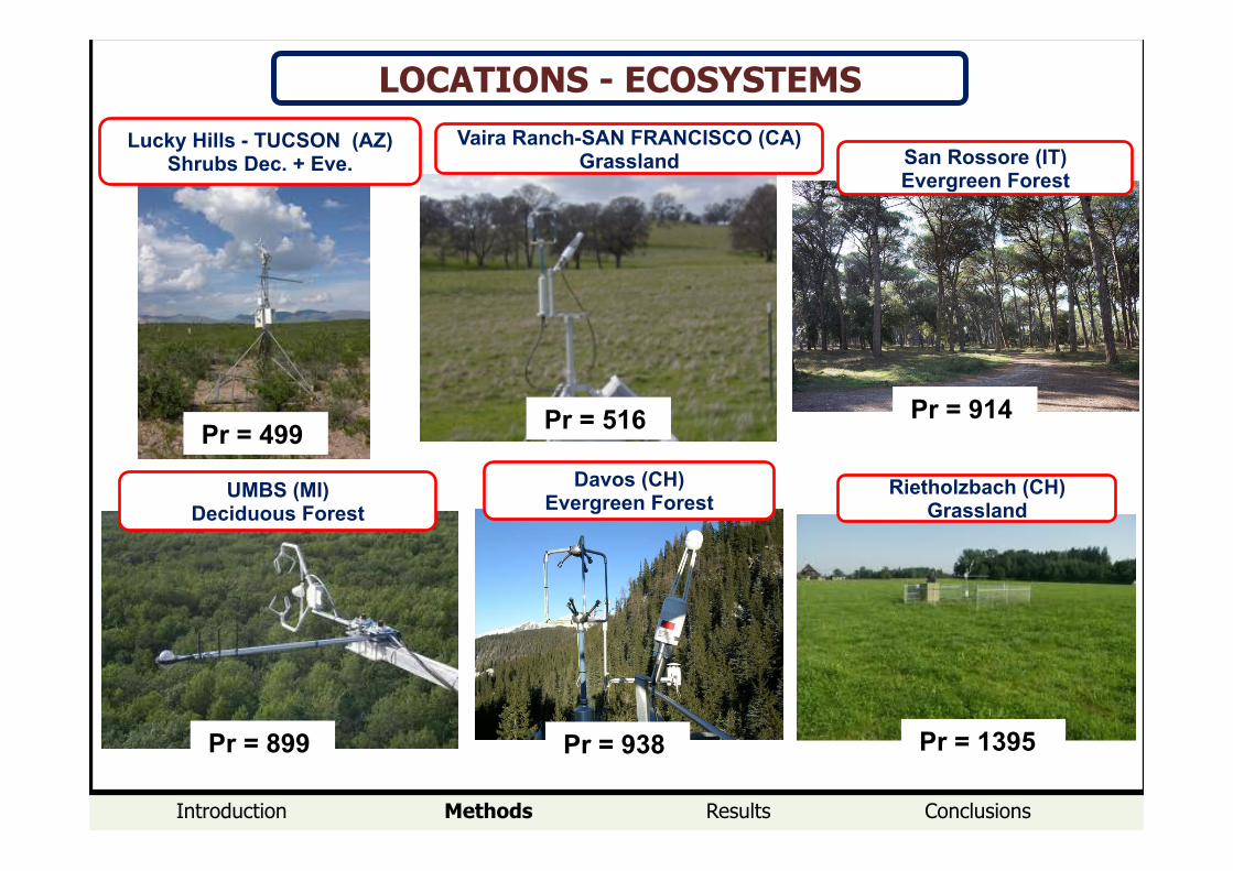
LOCATIONS - ECOSYSTEMS

Pr = 499!

Vaira Ranch-SAN FRANCISCO (CA) Grassland

UMBS (MI) Deciduous Forest

Lucky Hills - TUCSON (AZ) Shrubs Dec. + Eve.

Rietholzbach (CH) Grassland

Davos (CH) Evergreen Forest

San Rossore (IT) Evergreen Forest

Pr = 516! Pr = 914!

Pr = 899! Pr = 938! Pr = 1395!

Introduction Methods Results Conclusions

"me!evolu"on!of!the!spa"al!mean!

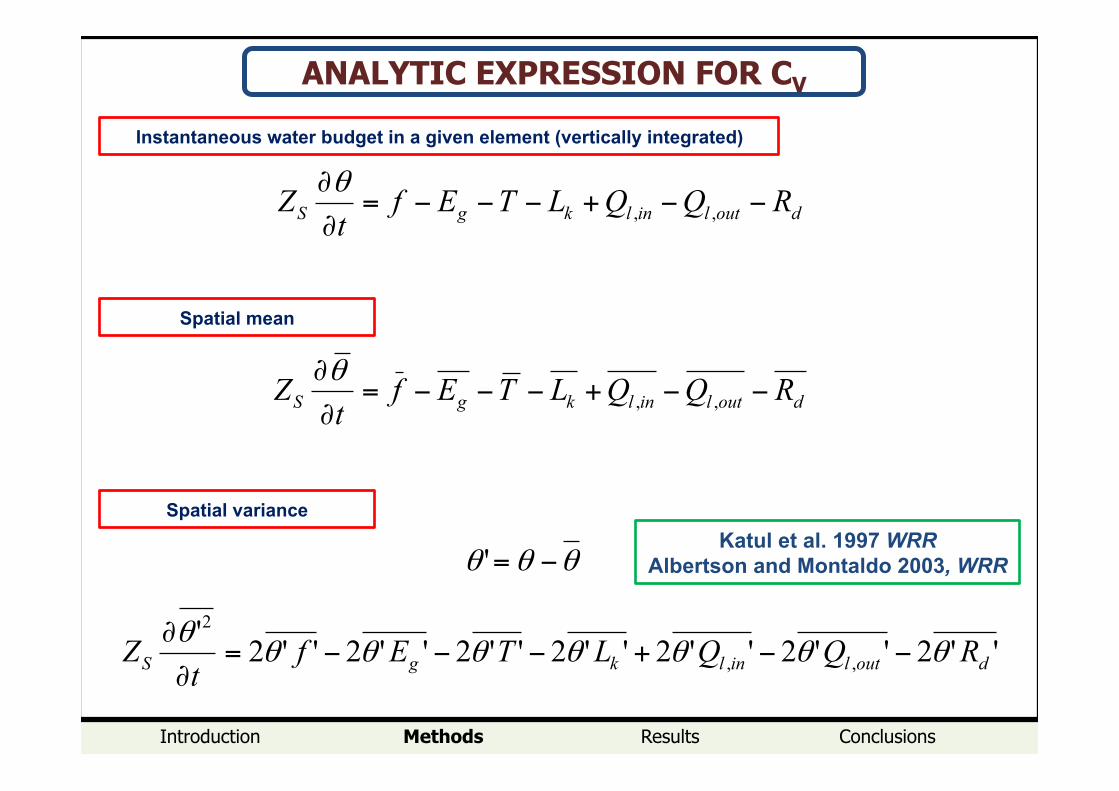
ANALYTIC EXPRESSION FOR CV

doutlinlkgS RQQLTEft

Z −−+−−−=∂∂

,,θ

doutlinlkgS RQQLTEft

Z −−+−−−=∂∂

,,θ

Instantaneous water budget in a given element (vertically integrated)

Spatial mean

Spatial variance

''2''2''2''2''2''2''2',,

2

doutlinlkgS RQQLTEft

Z θθθθθθθθ

−−+−−−=∂∂

θθθ −='Katul et al. 1997 WRR

Albertson and Montaldo 2003, WRR

Introduction Methods Results Conclusions

"me!evolu"on!of!the!spa"al!mean!

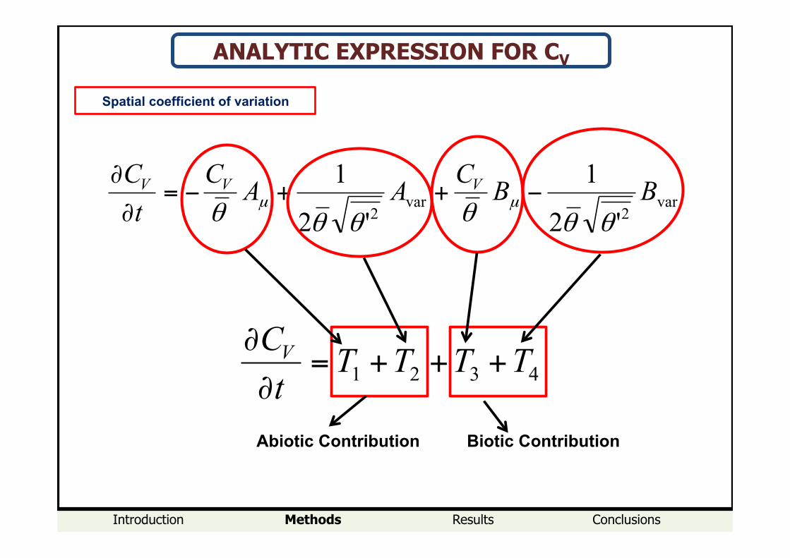
Spatial coefficient of variation

var2

var2 '2

1

'2

1 BBCAACtC VVV

θθθθθθ µµ −++−=∂∂

4321 TTTTtCV +++=∂∂

Abiotic Contribution! Biotic Contribution!

ANALYTIC EXPRESSION FOR CV

Introduction Methods Results Conclusions

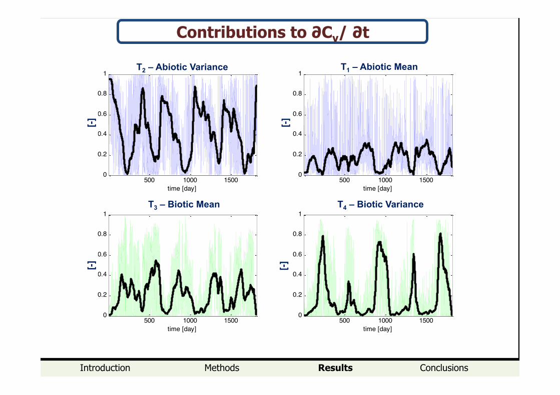
Contributions to ∂Cv/ ∂t

500 1000 15000

0.2

0.4

0.6

0.8

1

time [day]

[-]

T1 abiotic-var

500 1000 15000

0.2

0.4

0.6

0.8

1

time [day]

[-]

T2 abiotic-µ

500 1000 15000

0.2

0.4

0.6

0.8

1

time [day]

[-]

T3 biotic-µ

500 1000 15000

0.2

0.4

0.6

0.8

1

time [day]

[-]

T4 biotic-var

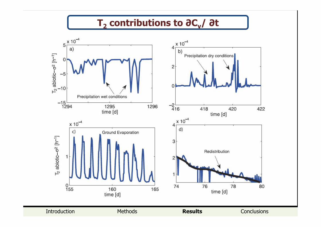
T2 – Abiotic Variance T1 – Abiotic Mean

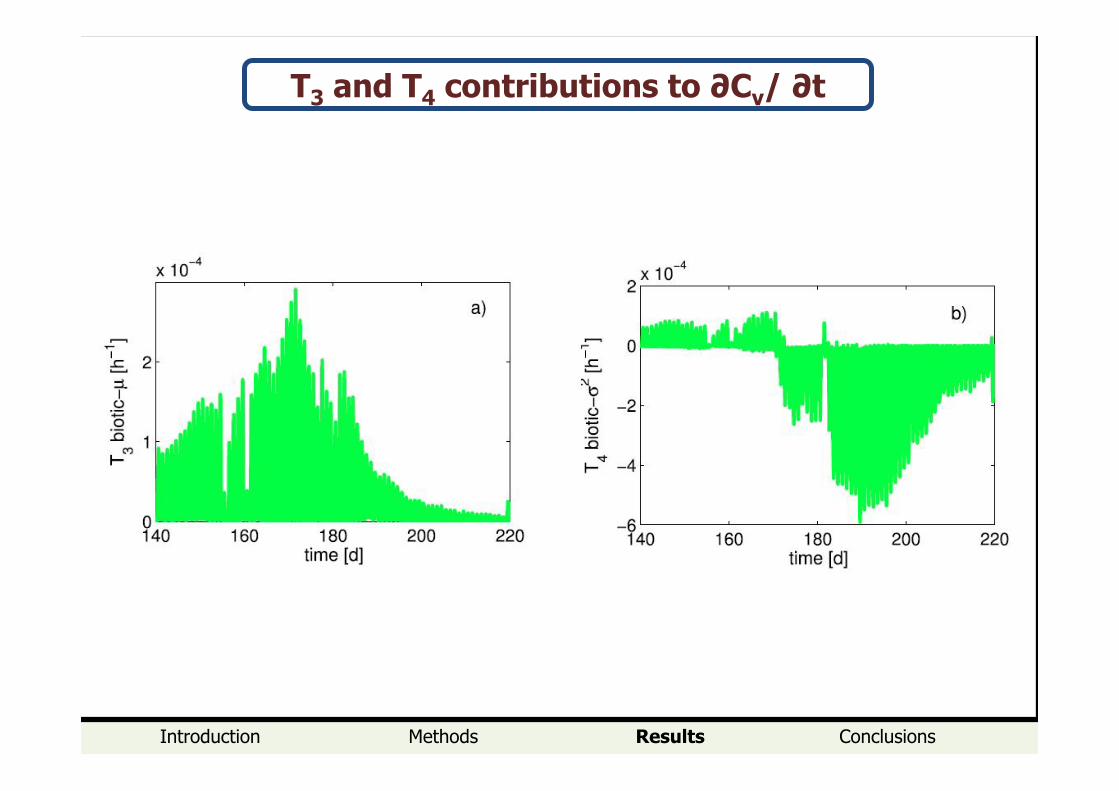
T3 – Biotic Mean T4 – Biotic Variance

[-]

[-]

[-]

[-]

Introduction Methods Results Conclusions

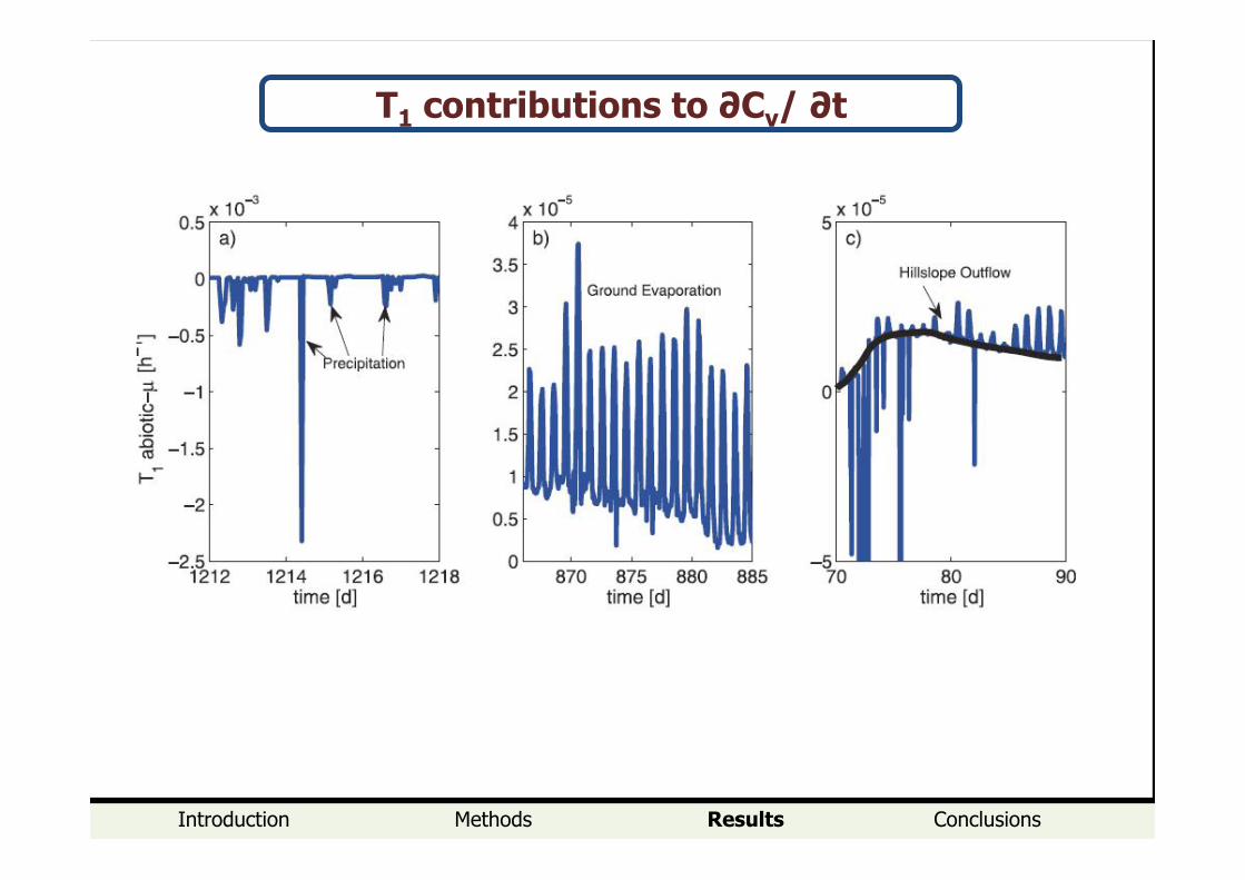
T1 contributions to ∂Cv/ ∂t

Introduction Methods Results Conclusions

T2 contributions to ∂Cv/ ∂t

Introduction Methods Results Conclusions

T3 and T4 contributions to ∂Cv/ ∂t

Introduction Methods Results Conclusions

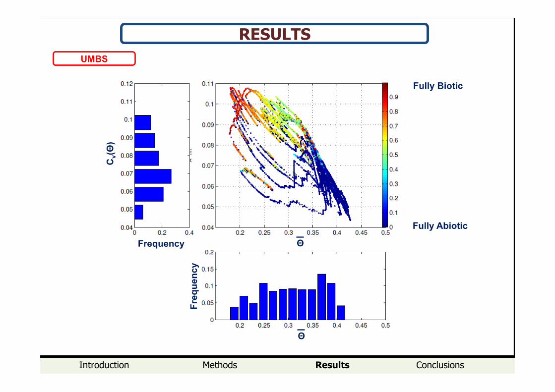
RESULTS UMBS

Θ

Cv(Θ

)

Frequency

Freq

uenc

y

Θ

Fully Biotic

Fully Abiotic

Results

Cv(Θ

)

Θ

Cv(Θ

) C

v(Θ

)

UMBS (MI)

DAVOS (CH)

RIETHOLZBACH (CH) SAN ROSSORE (IT)

VAIRA RANCH (CA)

LUCKY HILLS (AZ)

Θ

Cv(Θ

) C

v(Θ

) C

v(Θ

)

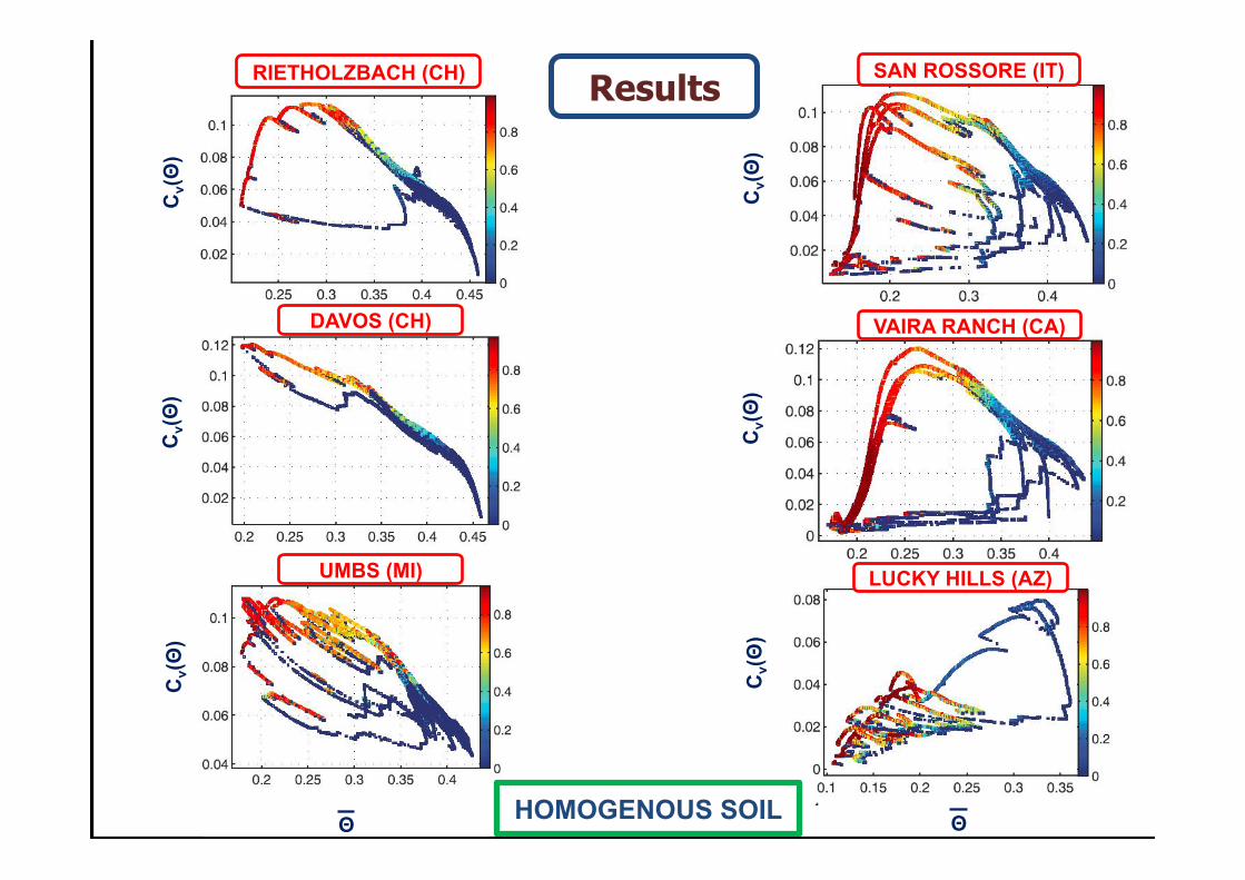
HOMOGENOUS SOIL

Results

Cv(Θ

)

Θ

Cv(Θ

) C

v(Θ

)

UMBS (MI)

DAVOS (CH)

RIETHOLZBACH (CH) SAN ROSSORE (IT)

VAIRA RANCH (CA)

LUCKY HILLS (AZ)

Θ

Cv(Θ

) C

v(Θ

) C

v(Θ

)

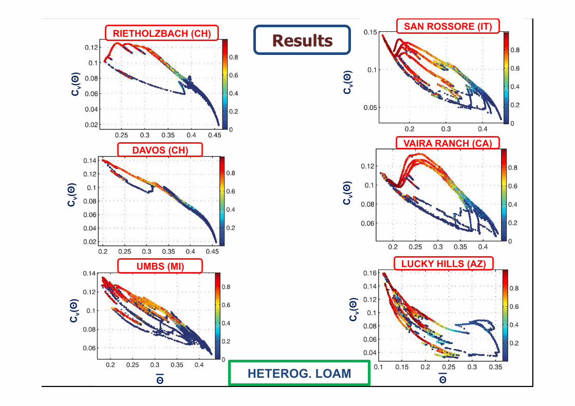
HETEROG. LOAM

Results C

v(Θ

)

Θ

Cv(Θ

) C

v(Θ

)

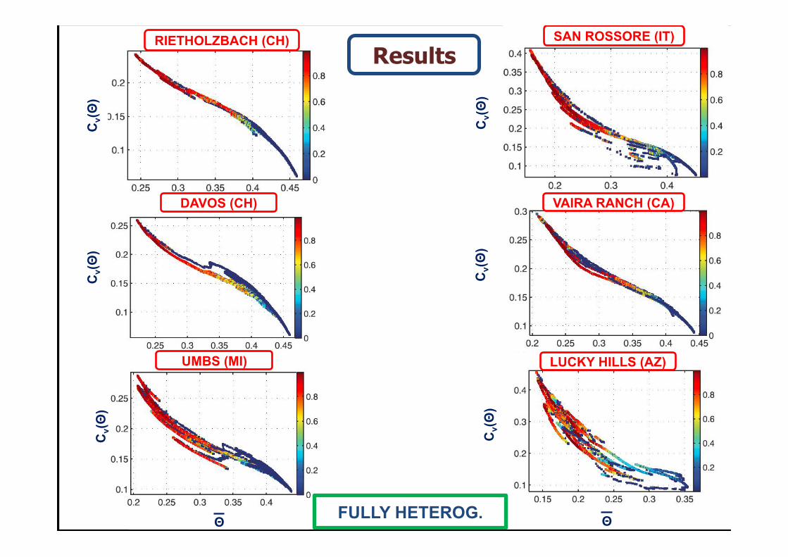
UMBS (MI)

DAVOS (CH)

RIETHOLZBACH (CH) SAN ROSSORE (IT)

VAIRA RANCH (CA)

LUCKY HILLS (AZ)

Θ

Cv(Θ

) C

v(Θ

) C

v(Θ

) FULLY HETEROG.

Introduction Methods Results Conclusions

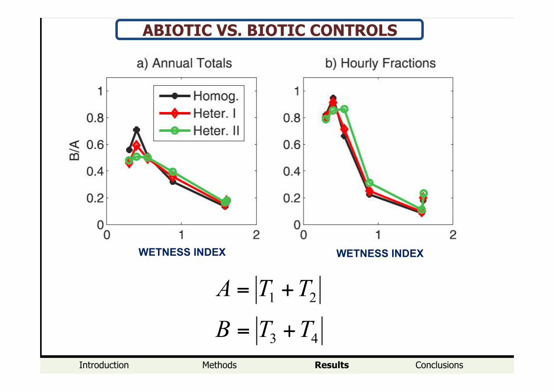
ABIOTIC VS. BIOTIC CONTROLS

43

21

TTB

TTA

+=

+=

WETNESS INDEX WETNESS INDEX

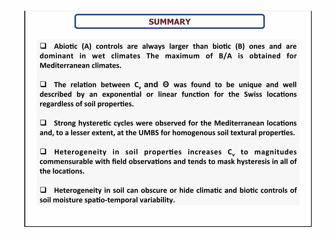
SUMMARY

!  Abio%c' (A)' controls' are' always' larger' than' bio%c' (B)' ones' and' are'dominant' in' wet' climates' The' maximum' of' B/A' is' obtained' for'Mediterranean'climates.'

!  The' rela%on' between' Cv' and Θ was' found' to' be' unique' and' well'described' by' an' exponen%al' or' linear' func%on' for' the' Swiss' loca%ons'regardless'of'soil'proper%es.''

!  Strong'hystere%c'cycles'were'observed'for'the'Mediterranean'loca%ons'and,'to'a'lesser'extent,'at'the'UMBS'for'homogenous'soil'textural'proper%es.''

!  Heterogeneity' in' soil' proper%es' increases' Cv' to' magnitudes'commensurable'with'field'observa%ons'and'tends'to'mask'hysteresis'in'all'of'the'loca%ons.'

!  Heterogeneity'in'soil'can'obscure'or'hide'clima%c'and'bio%c'controls'of'soil'moisture'spa%oItemporal'variability.''

Thanks for your attention !

Fatichi et al., 2015, WRR