Review of Tokamak Physics as a way to construct a device optimal for Graviton detection and generation within a confined small spatial volume, as opposed to Dyson’s “infinite astrophysical

Volume” calculations.

ANDREW WALCOTT BECKWITH

Physics department

Chongqing University College of Physics, Chongqing University Huxi Campus

No. 55 Daxuechen Nanlu, Shapingba District, Chongqing 401331

which is in Chinese:重庆市沙坪坝区大学城南路55号重庆大学虎溪校区

People’s Republic of China

Rwill9955b@gmail.com

Abstract: - Review of arguments in refutation of Dyson’s alleged prohibition against use of device physics as to determining if

Gravitons can be determined to exist is followed up by use of a hot Plasma within a Tokamak in a re do of the amplitude of alleged

Gravitational waves. This overlaps with gravitons, and we follow up with an analysis of the pertinent form of Gravitons, i.e. do we have

massless or massive gravitons. In addition we also obtain GW of amplitude as low as

26 27

2 1005

~ 10 10Temp

nd term T KeVmeters above Tokamak

h

five meters above the Tokamak center such low strain values are

extremely close to brane world GW, and strain values in early universe cosmology. This is after our device analysis. Using

Grischuk and Sachin (1975) amplitude for the GW generation due to plasma in a toroid, we generalize this result for Tokamak physics.

We obtain evidence for strain values up to 25 26

2 ~ 10 10nd termh

in a Tokamak center. These values are an order of magnitude

sufficient to allow for possible detection of gravitational waves. The critical breakthrough is in utilizing a burning plasma drift current,

which relies upon a thermal contribution to an electric field. Such low strain values are extremely close to brane world GW, and

strain values in early universe cosmology. We conclude with statements as to comparing our basic results with those of Yan-Gang Miao, Ying-Jie Zhao as to their generalized HUP which gives support to the suppositions given in our comparison of the

character of gravitons which are initially at the start of inflation versus those of our present era, as measured by the Tokamak

Key-Words: - Tokamak physics, confinement time (of Plasma), GW amplitude, Drift current

1. Review of the Dyson argument which we cite for use in Tokamaks.

Our first goal is to show that Dyson’s arguments as given in [1] as to the impossibility of Graviton detection no longer apply to Tokamaks. Note, Dyson in [1] derived criteria as to the probability one could obtain physical phenomenon theoretically modelled by the Gertsenshtein effect [2]. The Gertsenshtein effect [2] is the coupling of magnetic fields, gravitons, and photons. In the Dyson treatment [1] of the Gertsenshtein effect [2] , Dyson hypothesized distances up to many light years for an interaction of magnetic fields, gravitons and photons, for experimental signals which could be detected on the Earth’s surface. This assumed geometry of many light years distance lead to the predicted Gertshenshtein effect [2] unable to allow for graviton detection. In contrast to this assumed vast distances for the Gertshenshtein effect in reference [1], the author has devised via tokamak generation of gravity waves which is discussed in this article which lead to an interaction length of meters for the magnetic field, gravitons, and photons. The reduced length is due to the magnetic field which the gravitons interact with, being inside the detector itself, thereby insuring a 100 % probability for the Gertsenshtein effect occurring. This is commensurate with predictions given in reference

[3].The Tokamak example brings up an important point, that even if one wants to measure gravitational waves, the Gertshenshtein effect for gravitons, magnetic field, and photons is within the small 3 dimensional geometry of the detector, with an enormous magnetic field. To do this note that we are talking about a Tokamak of the type described in [4].Having the Gerteshenshtein effect in such a small volume dramatically raises the likelihood of detection of gravitons, via resultant photons being picked up by the 3DSR device which in this care would be put above the Tokamak given in [5]

2. Probability for the Gertsentshtein effect, as described by Dyson for the Tokamak GW

experiment.

We will briefly report upon Dyson’s well written summary results, passing by necessity to the part on the

likelihood of the Gertsenshtein effect occurring in a laboratory environment [1]. In doing so we put in specific

limits as to frequency and the magnetic field, since in our work the objective will be to have at least

theoretically a 100% chance of photon-graviton interaction [1] which is the heart of what Dyson reported in his

research findings. What we find, is that with a frequency of about 10 to the 9th Hertz and a magnetic field of 10

to the 9th Gauss that there is nearly 100% chance of the Gertsentshtein effect being observed, within the

confines of the Tokamak experiment as outlined in accommodating the geometrical considerations as related to

in references [4,5].

The Gertentshtein effect is linked to how there is a linkage, signal wise, between gravitons and photons, and we

are concerned as to what is a threshold as to insure that GW may be matched to the photons used by Dr. Li and

others [5] to signify GW in a detector . To do so let us look at the Dyson criteria as a minimum threshold for

the Gertentshtein effect happening [1], namely

2 4310D B (1)

The propagation distance is given by D, the magnetic field by B, and the frequency of gravitational radiation is

given by . We assume that the gravitational frequency is commensurate with the gravitational frequency of

gravitons, i.e. that they are, averaged out one and the same thing. In doing so, making use of [ 1 ] we suppose

on the basis of analysis that D is of the order of 10 to the 2nd power, since D is usually measured in centimetre,

and by [ 1] we are thinking of about a 1 meter If B is of the order of 10 to the 9th Gauss Hertz, as deemed

likely by the geometry as suited for [4], then we have that if the GW frequency , is likewise about 10 to

the 9th Hertz , that Eq.(1) is easy to satisfy. Note that if one has a vastly extended value for D, say 10 to the

13th centimetres that the inequality of Eq. (1) does not hold, so that by definition, as explained by Dyson that

in a lot of cases, not relevant to Tokamaks, that Eq. (1) is not valid, hence there would be no interexchange

between gravitons and photons, and hence, if applied to the Dr. Li detector [5] no way to measure gravitons by

their photonic signature. Fortunately, as given by considerations relevant to the geometry of the Tokamak this

extended version of D, say 10 to the 13th centimetres does not hold. And that then Eq. (1) holds. If so then, the

probability of the Gertentshtein effect is presentable as, approximately,

36 2 2 36 18 1810 10 10 10 ~ 1 100%P B (2)

Summing up Eq. (2) is that the chosen values, namely if D is of the order of 10 to the 2nd power, B is of the

order of 10 to the 9th power Gauss, and is likewise about 10 to the 9th Hertz leads to approximately 100%

chance of seeing Gertsenshtein effects in the planned Tokamak experiment as discussed in the 2nd part of this

manuscript. . In making this prediction as to Eq. (2), we can say that the left hand side, leading up to the

evaluation of P with a numerator equal to 10 to the 36th power will be about unity for the values of B detector

fields in Gauss (magnetic field) or the generated gravitational field frequency from the Tokamak, making

an enormous magnetic field in the GW detector itself mandatory, which would necessitate a huge cryogenics

effort, with commensurate machinery. Keep in mind that the GW detector is, as given in the 2nd part of this

article that if it is situated about five meters above the Tokamak, i.e. presumably the one in Hefei, PRC [4]

.Note, that, ironically, Dyson gets much smaller values of Eq. (2) than the above, by postulating GW

frequency inputs as to the value of about 10 to the 20th Hertz, i.e. our value of is likewise about

10 to the 9th Hertz, much lower. If one has such a high frequency, as given by Dyson, the of course,

Eq. (2) would then be close to zero for the probability of the Gertentshtein effect happening. I.e. our

analysis indicates that a medium high GW frequency, presumably close to 10 to the 9th Hertz, and D

10 to the 2nd power, presenting satisfaction of both Eq.(1) and Eq.(2). Note the main point though, for

large values of D, Eq. (1) will not hold, making Eq.(2) not relevant, and that means in terms of the Dyson

analysis, that far away objects generating gravitons will not be detectable. Via the Gertentshtein effect. There is

no such limitation due to a failure of Eq. (1) in the Tokamak GW generation setup since then, for Tokamaks, D

is very small. But if D is large in the case of a lot of astrophysical applications, then almost certainly one never

gets to Eq. (2) since the Gertsenshtein effect is ruled out. Having said that, we have our modus operandi, which

is to attempt to look at the way Plasma physics could lead to graviton and GW generation. This means looking

at [5], and also considering the phenomenology as given in [6] which of course is to be kept relevant to the

restrictions as given in [5,7]

3. Introduction to the Plasma physics.

Russian physicists Grishchuk and Sachin [8] obtained the amplitude of a Gravitational wave (GW) in a

plasma as

2 2

4

GA(amplitude GW) h ~ GWE

c (3)

This should be compared with [9] , and we can diagram the situation out as follows [10]

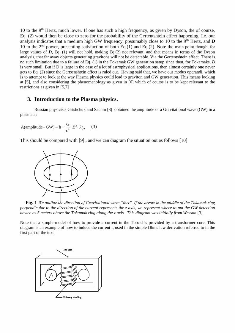
Fig. 1 We outline the direction of Gravitational wave “flux”. If the arrow in the middle of the Tokamak ring

perpendicular to the direction of the current represents the z axis, we represent where to put the GW detection

device as 5 meters above the Tokamak ring along the z axis. This diagram was initially from Wesson [3]

Note that a simple model of how to provide a current in the Toroid is provided by a transformer core. This

diagram is an example of how to induce the current I, used in the simple Ohms law derivation referred to in the

first part of the text

I I

I

Ion core

Primary winding

I

Ion core

Primary winding

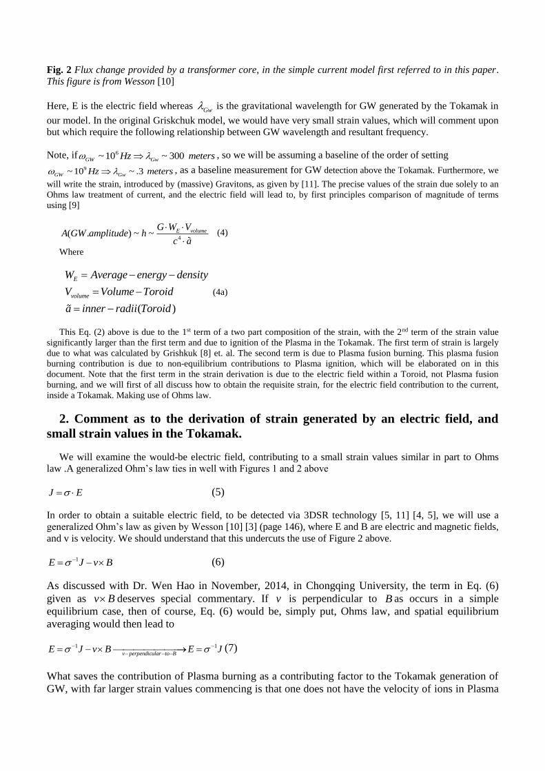
Fig. 2 Flux change provided by a transformer core, in the simple current model first referred to in this paper.

This figure is from Wesson [10]

Here, E is the electric field whereas Gw is the gravitational wavelength for GW generated by the Tokamak in

our model. In the original Griskchuk model, we would have very small strain values, which will comment upon

but which require the following relationship between GW wavelength and resultant frequency.

Note, if 6~10 ~ 300GW GwHz meters , so we will be assuming a baseline of the order of setting

9~ 10 ~ .3GW GwHz meters , as a baseline measurement for GW detection above the Tokamak. Furthermore, we

will write the strain, introduced by (massive) Gravitons, as given by [11]. The precise values of the strain due solely to an

Ohms law treatment of current, and the electric field will lead to, by first principles comparison of magnitude of terms

using [9]

4( . ) ~ ~ E volumeG W V

A GW amplitude hc a

(4)

Where

( )

E

volume

W Average energy density

V Volume Toroid

a inner radii Toroid

(4a)

This Eq. (2) above is due to the 1st term of a two part composition of the strain, with the 2nd term of the strain value

significantly larger than the first term and due to ignition of the Plasma in the Tokamak. The first term of strain is largely

due to what was calculated by Grishkuk [8] et. al. The second term is due to Plasma fusion burning. This plasma fusion

burning contribution is due to non-equilibrium contributions to Plasma ignition, which will be elaborated on in this

document. Note that the first term in the strain derivation is due to the electric field within a Toroid, not Plasma fusion

burning, and we will first of all discuss how to obtain the requisite strain, for the electric field contribution to the current,

inside a Tokamak. Making use of Ohms law.

2. Comment as to the derivation of strain generated by an electric field, and

small strain values in the Tokamak.

We will examine the would-be electric field, contributing to a small strain values similar in part to Ohms

law .A generalized Ohm’s law ties in well with Figures 1 and 2 above

J E (5)

In order to obtain a suitable electric field, to be detected via 3DSR technology [5, 11] [4, 5], we will use a

generalized Ohm’s law as given by Wesson [10] [3] (page 146), where E and B are electric and magnetic fields,

and v is velocity. We should understand that this undercuts the use of Figure 2 above.

1E J v B (6)

As discussed with Dr. Wen Hao in November, 2014, in Chongqing University, the term in Eq. (6)

given as v B deserves special commentary. If v is perpendicular to B as occurs in a simple

equilibrium case, then of course, Eq. (6) would be, simply put, Ohms law, and spatial equilibrium

averaging would then lead to

1 1

v perpendicular to BE J v B E J

(7)

What saves the contribution of Plasma burning as a contributing factor to the Tokamak generation of

GW, with far larger strain values commencing is that one does not have the velocity of ions in Plasma

perpendicular to B fields in the beginning of Tokamak generation. It is, fortunately for us, a non

equilibrium initial process, with thermal irregularities leading to both terms in Eq. (7) contributing to

the electric field values.

We will be looking for an application for radial free electric fields being applied e.g., Wesson [10] [3]

(page 120)

j

j j r j

dPn e E v B

dr (8)

Here, jn = ion density, jth species, je = ion charge, jth species, rE = radial electric field, jv = perpendicular

velocity, of jth species, B = magnetic field, and jP = pressure, jth species. The results of Eq. (5) and Eq. (6) are

22

2 2 2 2

4 4 4

G G G~ b

GW GW R GW

JConstE v

c c R c n e

= (1st) + (2nd) (9)

Here, the 1st term is due to 0E , and the 2nd term is due to 1j

n nn j j

dPE v B

dx n e

with the 1st term

generating 38 30~10 10h in terms of GW amplitude strain 5 meters above the Tokamak , whereas the 2nd

term has an 26~10h in terms of GW amplitude above the Tokamak. The article has contributions from

amplitude from the 1st and 2nd terms separately. The second part will be tabulated separately from the first

contribution assuming a minimum temperature of ~10T Temp KeV as from Wesson [10]

4. GW h strain values when the first term of Eq.(9) is used for different

Tokamaks

We now look at what we can expect with the simple Ohm’s law calculation for strain values. As it is,

the effort lead to non-usable GW amplitude values of up to 38 30~10 10h for GW wave amplitudes 5 meters

above a Tokamak, and 36 28~10 10h in the centre of a Tokamak. I.e. this would be using Ohm’s law and

these are sample values of the Tokamak generated GW amplitude, using the first term of Eq. (9) and obtaining

the following value [8] with a change as

2

2 2 2

4 4

G G~ ~First term GW GW

Jh E

c c

(9a)

We summarize the results of such in our first table as given for when 9~10 ~ .3GW GwHz meters and with

conductivity 2( ) ~10 sectokamak plasma m and with the following provisions as to initial values. What we observe are

a range of Tokamak values which are, even in the case of ITER (not yet built) beyond the reach of any technological

detection devices which are conceivable in the coming decade. This table and its results, assuming fixed conductivity

values 2( ) ~10 sectokamak plasma m as well as ~ .3Gw meters is why the author, after due consideration

completed his derivation of results as to the 2nd term of Eq. (9) which lead to even for when considering the results for the

Chinese Tokamak in Hefei to have[6]

2

2 2 2

4 4

G G~ ~ b

Second term GW R GW

Jh E v

c c n e

(10)

Or values 10,000 larger than the results in ITER due to Eq. (10).’

We summarize the results of such in our first table as given for when 9~10 ~ .3GW GwHz meters

and with information from Table 1 of Appendix A, so

View appendix A below which has useful data

Table 1: Values of strain at centre of Tokamak, and 5 meters above Tokamak:

Note that we are setting ~ .3Gw meters , 2( ) ~10 sectokamak plasma m , using Eq.(11) above for

Amplitude of GW.

What makes it mandatory to go the 2nd term of Eq. (11) is that even in the case of ITER, 5 meters above the

Tokamak ring, the GW amplitude is 1/10,000 the size of any reasonable GW detection device, and this

including the new 3DSR technology (Li et al, 2009) [5, 11] . Hence, we need to come up with a better

estimate, which is what the 2nd term of Eq. (7) is about which is derived in the next section

4 Enhancing GW strain Amplitude via utilizing a burning Plasma drift current:

Eq. (6)

The way forward is to go to Wesson, [10] (2011, page 120) and to look at the normal to surface

induced electric field contribution

1j

n nn j j

dPE v B

dx n e

(11)

If one has for Rv as the radial velocity of ions in the Tokamak from Tokamak centre to its radial

distance, R, from centre, and B as the direction of a magnetic field in the ‘face’ of a Toroid

containing the Plasma, in the angular direction from a minimal toroid radius of R a , with 0 , to

R a r with , one has Rv for radial drift velocity of ions in the Tokamak, and B having a net

approximate value of: with B not perpendicular to the ion velocity, so then [10]

~ Rnv B v B (12)

This should be considered within the constraints given by [11] as well as the geometry given in [12]

for the Hefei Tokamak.

Also, as a first order approximation: From Wesson [10] (page 167) the spatial change in pressure

denoted

j

b

n

dPB j

dx (13)

Here (ibid), the drift current, using a R , and drift current bj for Plasma charges, i.e.

1/2

~drift

b Temp

dnj T

B dr

(14)

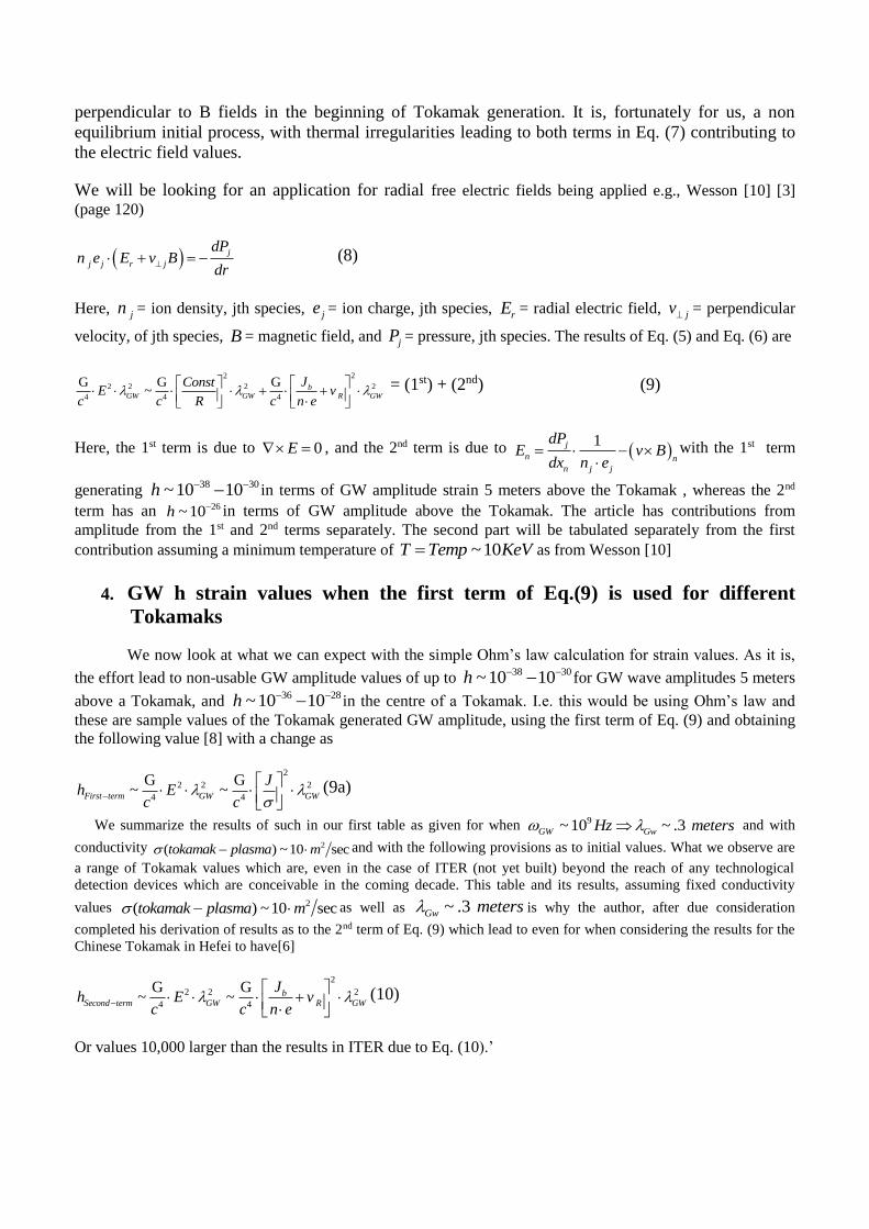
Figure 3 below introduces the role of the drift current, in terms of Tokamaks [10]

Fig. 3 Typical bootstrap currents with a shift due to r/a where r is the radial direction of the Tokamak, and a is

the inner radius of the Toroid This figure is reproduced from Wesson [10]

Then one has

2

2

1/4 22

2 2

1/4 2

2

~

1

1~

b j j

drift

j drift

drift

j drift

B j n e

dnB

e B n dr

dn

e n dr

(15)

Now, the behaviour of the numerical density of ions, can be given as follows, namely growing in the radial

direction, then [10]

expdrift drift initialn n r (16)

This exponential behaviour then will lead to the 2nd term in Eq. (9) having in the centre of the Tokamak, for an

ignition temperature of 10TempT KeV a value of

2

22 2

4

1/42 2

2 25

4 2

~

G

G~ ~ 10

nd term

b j j GW

Temp

GW

j

h

B j n ec

T

c e

(17)

As shown in Fig. 4 (copied from Wesson 2011), [10] there is a critical ignition temperature at its lowest point

of the curve in the having 30TempT KeV as an optimum value of the Tokamak ignition temperature for

20 3~ 10ionn m, with a still permissible temperature value of 100Temp safe upper bound

T KeV

with a value of

20 3~ 10ionn m, due to from page 11, [10] the relationship of Eq.(18), where

E is a Tokamak confinement of

plasma time of about 1-3 seconds, at least due to [10]

20 3.5 10 secion En m (18)

j b

P

0 0.2 0.4 0.6 0.8 1.0r/a

j b

P

0 0.2 0.4 0.6 0.8 1.0r/a

Fig. 4 The value of nE required to obtain ignition, as a function of temperature. Figure reproduced

from Wesson [10]

Also, as shown in Fig. 4, 100Temp safe upper boundT KeV

then one could have at the Tokamak centre, i.e.

even the Hefei based Tokamak [10,12]

2 100

1/42 2

2 25 26

4 2

~

G~ 10 10

Tempnd term T KeV

Temp

GW

j

h

T

c e

(19)

This would lead to, for a GW reading 5 meters above the Tokamak, then lead to for then the Hefei PRC

Tokamak [10, 12]

2 1005

1/42 2

2 27

4 2

G~ ~ 10

Tempnd term T KeV

meters above Tokamak

Temp

GW

j

h

T

c e

(20)

Note that the support for up to 100 KeV for temperature can yield more stability in terms of thermal Plasma

confinement as give in Fig. 5 below, namely from [10] we have

T (keV)10 100

(m-3s)

nE

T (keV)10 100

(m-3s)

nE

Power

L-mode

Ignition

H-mode

-particle

power

Conduction

loss

Equilibrium

Temperature

Power

L-mode

Ignition

H-mode

-particle

power

Conduction

loss

Equilibrium

Temperature

Power

L-mode

Ignition

H-mode

-particle

power

Conduction

loss

Equilibrium

Temperature

Fig 5 Illustrating how increase in temperature can lead to the H mode region, in Tokamak physics where the

designated equilibrium point, in Fig. 5 is a known way to balance conduction loss with alpha particle power,

which is a known way to increase E i.e. Tokamak confinement of plasma time [9]

5. Details of the model in terms of terms of adding impurities to the Plasma to get a longer

confinement time (possibly to improve the chances of GW detection).

We add this detail in, due to a question raised by Dr. Li who wished for longer confinement times for

the Plasma in order to allegedly improve the chances of GW detection for a detector 5 meters above

the Tokamak in Hefei. Wesson [10] (2011) stated that the confinement time may be made proportional

to the numerical density of argon/ neon seeded to the plasma [10] (page 180). This depends upon the

nature of the Tokamak, but it is a known technique, and is suitable for analysis, depending upon the

specifics of the Tokamak. I.e. this is a detail Dr. Li raised with his co-workers in Hefei, PRC in 2014

[12].

6. Restating the energy density and power which would be in the Hefei Tokamak, using

the formalism of Eq. (4) directly

1/42 22

2

1/42 2

2

2

~

~

TempGWE

volume j

Temp plasma fusion burning

E volume GW

j

TW

V e

TW V

e

(21)

The temperature for Plasma fusion burning, is then about between 30 to 100 KeV, as given by Wesson

[10]

The corresponding power as given by Wesson is then for the Tokamak [10]

0

BEP E J

R

(22)

The tie in with Eq. (20) by Eq. (22) can be seen by first of all setting the E field as related to the B

field, via E (electrostatic) ~ 12 110 Vm as equivalent to a magnetic field B ~ 410 ( )T Torr as given by [9].

In a one second interval, if we use the input power as an experimentally supplied quantity, then the

effective E field is

1/8

~applied okamak temperature

j

E Te

(23)

What is found is, that if Eq. (22) and Eq. (23) hold. Then by Wesson [10], pp. 242-243, if

0~1.5, ~1.5, / 3eff aZ q q R a Then the temperature of a Tokamak, to good approximation would be

between 30 to 100 KeV, and then one has [10]

4/5 ~ .87 Tokamak temperatureB T T (24)

Then the power for the Tokamak is

9/4

1/8

5/4

0 (.87)

okamak temperature

Tokamak toroidj

TP

e R

(25)

Then, per second, the author derived the following rate of production per second of a 3410 eV graviton, as given by, if / 3a R

/sec

1/4

2 1/8 2 2 5/4

0

2

3

(.87)

~ 1/

massive gravitons ond

okamak temperaturej

Graviton graviton

Graviton

n Tokamak

Te

R m c

scaling

(26)

If there is a fixed mass for a massive graviton, the above means that as the wavelength decreases, that

the number of gravitons produced between plasma burning temperatures of 30 to 100 KeV changes

dramatically. The change in graviton number is not nearly so sensitive as to Plasma fusion burning as

for 30 to 100 KeV temperature variation.

Numerical inputs into Eq. (26) have indicated that there are roughly 1000 gravitons per second

generated by Plasma fusion burning, with a strain value of 27~10h 5 meters above the centre of the

Hefei Tokamak[12]. If so, then the long confinement time of the Hefei Tokamak, for plasmas, would

indicate a chance that a detector may be able to obtain a graviton signal. That depends upon if 27~10h is, with the equipment available actually detectable. If so, then the next task is the extremely

time consuming process of experimental verification of the measurements, and answering questions as

to the reliability of the obtained data sets.

7 Looking at the role of Gravitons, in massless and massive gravity

configurations

We do note that there will be a complimentary relationship between presumed brane world generated GW [13],

which has the similar order of magnitude to the Tokamak generated GW and gravitons. Hence, due to [13] we

will bring up some material which is related to the nature of gravitons, from first principles.

Note that in the early universe, the following may be considered as complimentary, i.e. that we are looking at

material from [14, 15]. To start of with consider how to obtain massive gravitons, and to do that we start with

material from [16].

2

. 1Einstein Const Radius Universel (27)

Which in turn may help us understand when the formation of this value occurred, i.e. [17]

(2 (2

3 3

) )gravitonm

c

(28)

We are supposing that Eq. (27) and Eq. (28) holds at the formation of a Schwartzshield mass of the

Universe radius. Also, here is our candidate as to the formation of an initial time step. As given.

2/3

2 10~initial Planckt L

g N

(29)

Then, up to a point, if the above is in terms of seconds, and N sufficiently large, we could be talking

about an initial non zero entropy, along the lines of the number of nucleated particles, at the start of

the cosmological era. As given by making use of quantum infinite statistics as well as our adaptation

of it [18]

2/3

2 10( ) ~ ~ Planck

initial

S initial N n Lg t

(30)

Initial entropy would be small, but non zero, and would be affected by gstrongly, i.e. the initial

degrees of freedom assume would play a major role as far as how initial entropy and initial time steps

would be initiated. i.e. in this configuration, there is room then for in the early universe, a rest mass of

a graviton, of approximately 10^ -62 grams, which would tie an initial non zero entropy, as in Eq. 30,

with an initial time step, as given in Eq. 29, with the number, n ~ N of gravitons as given with mass

m, of Eq. (28), as possibly conferring information transfer, i.e. looking at what shows up as a

proportionality factor as far as how to obtain entropy is in having the following set up, i.e. if we look

eventually at the Schwartzhield radius of the universe as occurring at redshift z = 1000, about 300,000

years after the big bang, then

3

3

4

3Schwartzshield radii Universe

Universe QM effects BH

R

S

(31)

Furthermore, there is a linkage which can be made to Seth Lloyds number of operations, i.e. [16]

4/3 126

3

~1100(

3126

#( ) ~ ~ 10

4

3

4#( ) ~ 10

3

Universe

Z first light radii Universe

QM effects BH

operations S

R

operations

(32)

Whereas if t(initial ) ~ t (H) as given below

153~ ~ 10H

QM effects BH Planck

Planck

tL meters

t

(33)

The entropy of the universe, as given by S ~N , with the linkage as given by Ng. [19] would tie into

an initial frequency range, which would be extremely high, and that due to the smallness of the

wavelength, as given by Eq. (33) above.

If initial wavelength, as given by Eq.(33) is inversely proportional to an INITIAL version of energy,

then there could be a version of this affecting the mass of a graviton as given by ~ c , being re

written, as through use of Eq. (29) as of the rest mass of a graviton about Planck time leading to

2/3 3

min 2

32

2 2/3

1

( )~ ~ ~ ~

2 10 3

~

2 ( ) 10 1~

3

~ ( 1000)

Planck g

Planckg

initial entropy

c g N V volumec c t N

L m c

Entropy

V volume Lm

c g N N

S Before z

(31)

I.e. before Planck time, we would have the graviton mass as effectively zero, and it would about the

time of Planck time, scale as given in Eq. (31) with graviton rest mass eventually being in tandem

with Eq. (28)

Then, if the following hold before and after Planck time [18]

0,

1,

0;

) )(2 (2

3 3

(2

3

;

)

graviton

Planck Planck

Planck Planck

g Planck

today

Planck

Plan

gravito

ck today

n

t t t

m

t

c

mc

t t t t

m t t

t t

t t

(32)

Eq. (31) and Eq. (32) define the range of values of the Planck mass, as given, and also, the Pre Octonionic ( Pre

Planckian time) regime to Planckian time regime as given by

What we are considering is the following transformation, simply put. And this will be hopefully

detected by a change in phase, given by use of reference [6] style phase 0

In addition we use [19]

0 ,

Pr

change in phase given byp ph

tt e Octonionic

Octonionic

t

ase

t

t Eg

t E

with t FIXEDg E

(33)

8. Now about conditions to obtain the relevant data for phase 0

This paper examines geometric changes that occurred in the earliest phase of the universe, leading to values for

data collection of information for phase 0 , and explores how those geometric changes may be measured

through gravitational wave data. The change in geometry is occurring when we have first a pre quantum space

time state, in which, in commutation relations [20] (Crowell, 2005) in the pre Octionic space time regime no

approach to QM commutations is possible as seen by Eq.(34), i.e in Pre Octonionic, Pre Planckian space time

[20]

ipx jj ,

(34)

In the situation when we approach quantum “octonionic gravity applicable” geometry, Eq. (34) becomes

[20]

ipx jj ,

(35)

Having said that, if Gravitons are from the early electro weak era, in terms of production, in early universe

conditions, the situation is definable via [15]

We will elaborate upon this, but we have to state that purely massless gravitons are commensurate with the Pre

Planckian era, and that conditions given in [14] hold.

I.e. for the Tokamak, we are working with the present day era of Eq. (32) given above.

8. Examination of our write up about gravitons and the tie in with the HUP, and

cosmological constant with the work of Yan- Gang Miao, and Ying-Jie Zhao

In [21] there is a use of a relationship between the size of a spatial interval of space-time and the cosmological

constant. What is of interest, is that due to what the authors call a suppression index, which they call ‘n’, that

the authors up to a point partially confirm the results we have been talking of. I.e., the difference is that they

use their results to confirm the existence of a cosmological constant in its present value, but do not discuss the

pre Planckian space-time considerations we have brought up. It is of note though that their suppression index,

‘n’ is of the magnitude of present day estimations of entropy (if we take Entropy as a counting of ‘particles’ in

space-time). In doing so, we take note that the ‘suppression’ index so obtained was of the order of 10^121,

which is according to [22] tied into estimations of early to late space-time dynamics, which is given credence in

[23]. The noteworthy matter to bring to the attention of the readers is that there is in formula 10 of reference

[21] an explicit “vacuum energy” expression, which has the minimum length, delta x, of the order of Planck’s

length as part of a formula leading to “vacuum energy” in formula 10 of reference [21] which is presumed to be

of the magnitude of the Cosmological ‘constant’. Left unsaid though is then the derivation of the factor ‘n’ as

part of a ‘suppression’ meme of reducing an initially huge energy value, by 10^-121 as given in Eq. (11) of

reference [21]. However in dong so, the factor ‘n’ has the value of 10^123 which the authors then say was

corrected to be of the value of 10^121.

Here is the take away. If one is making the identification of S~ ‘n’, as in a counting algorithm, for entropy

along the lines of Ng’s infinite quantum statistics, as given in [18], then the suppression factor ‘n’ is of the

magnitude of the present entropy of the universe which could be predicted via following [22, 23]. Hence, we

make the following identification, namely following [18, 21]

S (entropy, today) ~ N(counting factor) ~ ‘n’ (suppression factor) ~ 10^121 (37)

If we literally took this as gospel, we would be assuming the existence of an enormous suppression factor index

‘n’ would be enough if in tandem with entropy, to state, if ‘n’ were fixed, that we would have the existence of a

cosmological constant of today’s value, if formula 10 of reference [21] held. Needless to say though if ‘n’ ~ N

~ entropy (early universe) were considerably smaller than 10^121, then the cosmological ‘constant’ of the early

universe would be considerably larger than what it is today. By many orders of magnitude.

The equations in question from [21] reads as follows, namely

:min

' '

4 2/' '2

' '121 123

2/' '

121 123

~ ~

2 3,

' ' 2~ ~

38

& ~

2 3,

' ' 2~ 10 10

3

' ' ~ 10 10 ( )

Planck

n

n

n

n

X l

c nvacuum energy

today

niff

n S entropy today

(38)

The vacuum energy in question is the same as the cosmological constant, if and only if the factor ‘n’ is

so enormous. Aside from the numerology , which is suggestive, there is a basic inconsistency which

we wish to find an answer to because the ‘vacuum energy’ starts off with a Planck’s length, but the

presumed 121 123' ' ~10 10 ( )n S entropy today suggests Planckian physics.

We wish to find a resolution between this apparent inconsistency in future work, but we applaud the insight of

[21] as linking ‘vacuum energy’, ‘n’ and the minimum length, which is in their estimation Planck length.

Needless to say, up to a point they may be arguing for ‘quintessence’ if much smaller ‘n’ as N which is

proportional to early universe entropy existed. We do know though by the supernova candle, that by the time of

the formation of the first stars, that the cosmological ‘constant’ was stable and of the same value as of the

present era. This is a topic which the research group is well aware of and which deserves specific study and

review.

9. Conclusion. GW generation due to the Thermal output of Plasma burning

Further elaboration of this matter in the experimental detection of experimental data sets for massive

gravity lies in the viability of the expression derived, namely Eq. (21)

. 27~10h for a GW detected 5 meters above a Tokamak represents the extreme limits of what could

be detected, but it is within the design specifications of what Dr. Li et al. (2009)[4,5] presented for

PRD readership. The challenge, as frankly brought up in discussions in Chongqing University is to

push development of 3DSR hardware to its limits, and use the Hefei Tokamak configuration as a test

bed for the new technology embodied in the Plasma fusion burning generation of Gravitation waves.

The importance of the formulation is in the explicit importance of temperature. I.e. a temperature

range of at least10 100TempKeV T KeV . In making this range for Eq. (25), care must also be taken

to obtain a sufficiently long confinement time for the fusion plasma in the Tokamak of at least 1

second or longer, and this is a matter of applied engineering dependent upon the instrumentation of

the Tokamak in Hefei, PRC.

Furthermore, .Wen, Li, and Fang, proved in [13] the likelihood of brane world generation of HFGW

which are close to the values of strain and frequency which could be generated by the Tokamak

described above. ‘

We also should be aware, of taking consideration of the extreme non linearity of the conductivity of

plasmas as discussed in [24] as the kinks and irregularities in the magnetic field, are a serious

contributor to the irregularities in the MHD simulations which will be part of a future study, of the

effects of gravity wave and graviton generation later on.

Acknowledgements

Gary Stevenson was largely responsible for the inputs of Appendix A, and Amara Angelica also asked

questions as to engineering issues which lead to the formulation of the equations in this document. Thanks to

both of them for cleaning many parts of the Tokamak work so presented. Also, several of the diagrams came

directly from Gary Stevenson, as illustrations of engineering concepts used in section 3 of this document.

The author thanks. Dr. Yang Xi whom imbued the author with the background in the U of Houston to obtain a

doctorate in physics Also, my recently deceased father is thanked whom discussed decades ago with me as to

the worth of five dimensional geometry, in cosmology. Also, the Chongqing University physics department is

thanked for the affiliation which has led to this article being formed in the first place for review, and that also

Dr. Fangyu Li, who encouraged me to explore such issues. This work is supported in part by National Nature

Science Foundation of China grant No. 11375279

References:

[1] FREEMAN DYSON, Int. J. Mod. Phys. A, 28, 1330041 (2013) [14 pages] DOI:

10.1142/S0217751X1330041X

[2] M. E. Gertsenshtein, 1961. \Wave Resonance of Light and Gravitational Waves", JETP,41, 113-114, English translation in Soviet

Physics JETP, 14, 84-85 (1962).

[3] F. Li, F., M. Tang, M., D. Shi. “Electromagnetic response of a Gaussian beam to high frequency relic gravitational waves in

quintessential inflationary models”, PRD 67,104008 (2003), pp1-17

[4] J. Li, H. Y. Guo, et.al.” A long-pulse high-confinement plasma regime in the Experimental Advanced Superconducting

Tokamak”, Nature Physics (2013) doi:10.1038/nphys2795; Received 17 April 2013 Accepted 24 September 2013 Published online 17 November 2013 [5] F.Y. Li et al., Phys. Rev. D 80, 064013 (2009), arxiv re-qc/0909.4118 (2009)

[6] F. Li F., and N. Yang, “Phase and Polarization State of High Frequency Gravitational waves”, Chin Phys. Lett. Vol 236, No

5(2009), 050402, pp 1-4

[7] M. Maggiore, Gravitational Waves: Volume 1. Theory and Practice Oxford University press, 2008, Oxford UK

[8] L.P. Grishchuk, M.V. Sazchin “Excitation and Detection of Standing Gravitational Waves”, Zh. Eksp. Theor. Fiz 68, pp 1569-1582

(1975) Moscow

[9] F. Li, l M. Tang, J. Luo, and Y-C. Li, “Electrodynamical response of a high energy photon flux to a gravitational wave”, Phys. Rev. D. 62, 44018, (2000) [10] J. Wesson; “Tokamaks”, 4th edition, 2011 Oxford Science Publications, International Series of Monographs on Physics, Volume

149

[11] [R.C. Woods et al, Journal of Modern physics 2, number 6, starting at page 498, (2011)

[12] J. Li,et al, “ A Long Pulse high Confinement Plasma regime in the experimental Advanced Super conducting Tokamak”, Nature

Physics (2013), doi 10.1038/ nphys 2795, Published November 17, 2013

[13] H. Wen, F. Li, and Z. Fang “Electromagnetic response produced by interaction of high-frequency gravitational waves from brane

world with galactic-extragalactic magnetic fields” PR D 89, 104025, Published May 14, 2014

[14] Beckwith, A. (2016) Gedanken Experiment Examining How Kinetic Energy Would Dominate Potential

Energy, in Pre-Planckian Space-Time Physics, and Allow Us to Avoid the BICEP 2 Mistake. Journal of High Energy Physics, Gravitation and Cosmology, 2, 75-82. doi: 10.4236/jhepgc.2016.21008.

[15] A. Beckwith, Open Journal of Microphysics, 2011, 1, 13-18

doi:10.4236/ojm.2011.11002 Published Online

May 2011 (http://www.SciRP.org/journal/ojm)

[16] Ali, A.F. and Das, S. (2015) Cosmology from Quantum Potential. Physics Letters B, 741, 276-279.

[17] Haranas, I. and Gkigkitzis, I. (2014) “The Mass of Graviton and Its Relation to the Number of Information According to the

Holographic Principle”. International Scholarly Research Notices, 2014, Article ID: 718251.

http://www.hindawi.com/journals/isrn/2014/718251/

[18] Jack Ng, Y. (2008) Space-Time Foam: From Entropy and Holography to Infinite Statistics and Nonlocality. Entropy, 10, 441-461.

http://dx.doi.org/10.3390/e10040441

[19] Beckwith, A. (2016) Gedanken Experiment for Refining the Unruh Metric Tensor Uncertainty Principle via

Schwarzschild Geometry and Planckian Space-Time with Initial Nonzero Entropy and Applying the Riemannian-Penrose Inequality and Initial Kinetic Energy for a Lower Bound to Graviton Mass (Massive Gravity). Journal of High Energy Physics, Gravitation and Cosmology, 2, 106-124. doi: 10.4236/jhepgc.2016.21012. [20] Crowell, L., “Quantum Fluctuations of Space Time “, World Scientific Series in Contemporary Chemical Physics, Vol 25, World

Scientific, PTE, LTD, 2005, Singapore

[21] Yan-Gang Miao, Ying-Jie Zhao , “Interpretation of the Cosmological Constant Problem within the Framework of

Generalized Uncertainty Principle”, Int. J. Mod. Phys. D 23 (2014) 1450062, http://arxiv.org/abs/1312.4118

[22] Damien A. Easson, Paul H. Frampton, George F. Smoot, “Entropic Accelerating Universe”, Phys.Lett.B696:273-277,

2011, http://arxiv.org/abs/1002.4278 [23] Alexander Shalyt-Margolin, “Entropy in the Present and Early Universe: New Small Parameters and Dark Energy Problem”,

Entropy 2010, 12, 932-952; doi: 10.3390/e12040932

[24] Hirshman, S.:P, Hawruluk, R. J. and Birge, B. “Neoclassical conductivity of a Tokamak Plasma” Nuclear Fusion 17, 611 (1977)

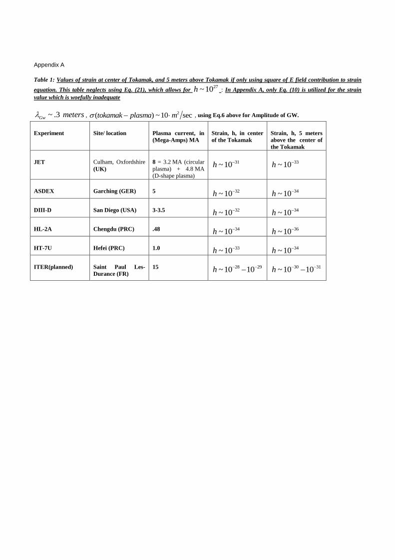
Appendix A

Table 1: Values of strain at center of Tokamak, and 5 meters above Tokamak if only using square of E field contribution to strain

equation. This table neglects using Eq. (21), which allows for 27~10h : In Appendix A, only Eq. (10) is utilized for the strain

value which is woefully inadequate

~ .3Gw meters , 2( ) ~10 sectokamak plasma m , using Eq.6 above for Amplitude of GW.

Experiment Site/ location Plasma current, in

(Mega-Amps) MA

Strain, h, in center

of the Tokamak

Strain, h, 5 meters

above the center of

the Tokamak

JET Culham, Oxfordshire

(UK)

8 = 3.2 MA (circular

plasma) + 4.8 MA

(D-shape plasma)

31~10h

33~10h

ASDEX Garching (GER) 5 32~10h

34~10h

DIII-D San Diego (USA) 3-3.5 32~10h

34~10h

HL-2A Chengdu (PRC) .48 34~10h

36~10h

HT-7U Hefei (PRC) 1.0 33~10h

34~10h

ITER(planned) Saint Paul Les-

Durance (FR)

15 28 29~10 10h 30 31~10 10h